On Distributions of Functionals of Anomalous Diffusion Paths

J Stat Phys (2010) 141: 1071–1092DOI 10.1007/s10955-010-0086-6

On Distributions of Functionals of Anomalous DiffusionPaths

Shai Carmi · Lior Turgeman · Eli Barkai

Received: 9 April 2010 / Accepted: 22 October 2010 / Published online: 4 November 2010© Springer Science+Business Media, LLC 2010

Abstract Functionals of Brownian motion have diverse applications in physics, mathemat-ics, and other fields. The probability density function (PDF) of Brownian functionals sat-isfies the Feynman-Kac formula, which is a Schrödinger equation in imaginary time. Inrecent years there is a growing interest in particular functionals of non-Brownian motion,or anomalous diffusion, but no equation existed for their PDF. Here, we derive a fractionalgeneralization of the Feynman-Kac equation for functionals of anomalous paths based onsub-diffusive continuous-time random walk. We also derive a backward equation and a gen-eralization to Lévy flights. Solutions are presented for a wide number of applications includ-ing the occupation time in half space and in an interval, the first passage time, the maximaldisplacement, and the hitting probability. We briefly discuss other fractional Schrödingerequations that recently appeared in the literature.

Keywords Continuous-time random-walk · Anomalous diffusion · Feynman-Kacequation · Levy flights · Fractional calculus

1 Introduction

A Brownian functional is defined as A = ∫ t

0 U [x(τ)]dτ , where x(t) is a trajectory of aBrownian particle and U(x) is a prescribed function [1]. Functionals of diffusive motionarise in numerous problems across a variety of scientific fields from condensed matterphysics [2–4], to hydrodynamics [5], meteorology [6], and finance [7, 8]. The distributionof these functionals satisfies a Schrödinger-like equation, derived in 1949 by Kac inspiredby Feynman’s path integrals [9]. Denote by G(x,A, t) the joint probability density function

S. Carmi (�) · L. Turgeman · E. BarkaiDepartment of Physics and Advanced Materials and Nanotechnology Institute, Bar-Ilan University,Ramat Gan 52900, Israele-mail: [email protected]

E. Barkaie-mail: [email protected]

mailto:[email protected]

mailto:[email protected]

1072 S. Carmi et al.

(PDF) of finding, at time t , the particle at x and the functional at A. The Feynman-Kactheory asserts that (for U(x) > 0) [1, 9]

∂

∂tG(x,p, t) = K

∂2

∂x2G(x,p, t) − pU(x)G(x,p, t), (1)

where the equation is in Laplace space, A → p, and K is the diffusion coefficient.The celebrated Feynman-Kac equation (1) describes functionals of normal Brownian mo-

tion. However, we know today that in a vast number of systems the underlying processesexhibit anomalous, non-Brownian sub-diffusion, as reflected by the nonlinear relation:〈x2〉 ∼ tα , 0 < α < 1 [10–14]. While a few specific functionals of anomalous paths havebeen investigated [15, 16], a general theory is still missing.

Several functionals of anomalous diffusion are of interest. For example, the time spentby a particle in a given domain, or the occupation time, is given by the functionalA = ∫ t

0 U [x(τ)]dτ , where U(x) = 1 in the domain and is zero otherwise [17–20]. Sucha functional can be used in kinetic studies of chemical reactions that take place exclu-sively in the domain. Consider for example a particle diffusing in a medium containingan interval that is absorbing at rate R. The average survival probability of the particle is〈exp(−RA)〉 [21]. Two other related functionals are the occupation time in the positivehalf-space (U(x) = �(x)) and the local time (U(x) = δ(x)) [15, 16, 22–24].

Another interesting family of functionals arises in the study of NMR [25]. In a typi-cal NMR experiment, the macroscopic measured signal can be written as E = 〈eiϕ〉 whereϕ = γ

∫ t

0 B[x(τ)]dτ is the phase accumulated by each spin, γ is the gyromagnetic ratio,B(x) is a spatially-inhomogeneous external magnetic field, and x(τ) is the trajectory ofeach particle. NMR therefore indirectly encodes information regarding the motion of theparticles. Common choices of the magnetic field B are B(x) = x and B(x) = x2 [25]. Fordispersive systems with inhomogeneous disorder where the motion of the particles is non-Brownian, the phase ϕ is a non-Brownian functional with U(x) = x or U(x) = x2.

In this paper, we develop a general theory of non-Brownian functionals. The processwe consider as the mechanism that leads to non-Brownian transport is the sub-diffusivecontinuous-time random-walk (CTRW). This is an important and widely investigatedprocess that is frequently used to describe the motion of particles in disordered systems[10–12, 26, 27]. In the scaling limit of this process, we derive the following fractionalFeynman-Kac equation:

∂

∂tG(x,p, t) = Kα

∂2

∂x2D1−α

t G(x,p, t) − pU(x)G(x,p, t), (2)

where the symbol D1−αt is Friedrich’s substantial fractional derivative and is equal in

Laplace space t → s to [s + pU(x)]1−α [28]. In the rest of the paper, we derive (2) andits backward version and then investigate applications for specific functionals of interest.A brief report of part of the results has recently appeared in [29].

2 Derivation of the Equations

We use the continuous-time random-walk (CTRW) model as the underlying process lead-ing to anomalous diffusion [10–12, 26, 27]. In CTRW, an infinite one-dimensional latticewith spacing a is assumed, and allowed jumps are to nearest neighbors only and with equalprobability of jumping left or right. Waiting times between jump events are independent

Functionals of Anomalous Diffusion Paths 1073

identically distributed random variables with PDF ψ(τ), and the process starts with a par-ticle at x = x0. The particle waits at x0 for time τ drawn from ψ(τ) and then jumps withprobability 1/2 to either x0 +a or x0 −a, after which the process is renewed. We assume thatno external forces are applied and that for long waiting times, ψ(τ) ∼ Bατ

−(1+α)/|(−α)|.For 0 < α < 1, the average waiting time is infinite and the process is sub-diffusive with〈x2〉 = 2Kαt

α/(1 + α) (Kα = a2/(2Bα), units m2/secα) [30]. We look for the differentialequation that describes the distribution of functionals in the scaling limit of this model.

2.1 Derivation of the Fractional Feynman-Kac Equation

Recall that the functional is defined as A = ∫ t

0 U [x(τ)]dτ and that G(x,A, t) is the jointPDF of x and A at time t . For the particle to be at (x,A) at time t , it must have beenat [x,A − τU(x)] at the time t − τ immediately after the last jump was made. LetQn(x,A, t)dt be the probability of the particle to make its nth jump into (x,A) in the timeinterval [t, t + dt]. Thus,

G(x,A, t) =∫ t

0W(τ)

∞∑

n=0

Qn[x,A − τU(x), t − τ ]dτ, (3)

where W(τ) = 1 − ∫ τ

0 ψ(τ ′)dτ ′ is the probability for not moving in a time interval oflength τ .

To arrive into (x,A) after n + 1 jumps, the particle must have arrived after n jumps intoeither [x − a,A − τU(x − a)] or [x + a,A − τU(x + a)], where τ the time between thejumps. Since the probabilities of jumping left and right are equal, we can write a recursionrelation for Qn:

Qn+1(x,A, t) =∫ t

0ψ(τ)

{1

2Qn[x + a,A − τU(x + a), t − τ ]

+ 1

2Qn[x − a,A − τU(x − a), t − τ ]

}

dτ, (4)

where ψ(τ) is the PDF of τ , the time between jumps. For n = 0 (no jumps were made),Q0 = δ(x − x0)δ(A)δ(t).

Assume that U(x) ≥ 0 for all x and thus A ≥ 0 (an assumption we will relax later). LetQn(x,p, t) be the Laplace transform A → p of Qn(x,A, t)—we use along this work theconvention that the variables in parenthesis define the space we are working in. We note that

∫ ∞

0e−pAQn[x,A − τU(x), t]dA = e−pτU(x)

∫ ∞

0e−pA′

Qn(x,A′, t)dA′

= e−pτU(x)Qn(x,p, t),

where we used the fact that Qn(x,A, t) = 0 for A < 0. Thus, Laplace transforming A → p

equation (4) we find

Qn+1(x,p, t) = 1

2

∫ t

0ψ(τ)e−pτU(x+a)Qn(x + a,p, t − τ)dτ

+ 1

2

∫ t

0ψ(τ)e−pτU(x−a)Qn(x − a,p, t − τ)dτ. (5)


Laplace transforming t → s equation (5) using the convolution theorem,

Qn+1(x,p, s) = 1

2ψ[s + pU(x + a)]Qn(x + a,p, s)

+ 1

2ψ[s + pU(x − a)]Qn(x − a,p, s), (6)

where ψ(s) is the Laplace transform of the waiting time PDF. Fourier transforming x → k

equation (6),

Qn+1(k,p, s) = cos(ka)

∫ ∞

−∞eikxψ[s + pU(x)]Qn(x,p, s)dx.

Applying the Fourier transform identity F {xf (x)} = −i ∂∂k

f (k),

Qn+1(k,p, s) = cos(ka)ψ

[

s + pU

(

−i∂

∂k

)]

Qn(k,p, s). (7)

Note that the order of the terms is important: ψ[s + pU(−i ∂∂k

)] does not commute withcos(ka). Summing (7) over all n, using the initial condition Q0(k,p, s) = eikx0 , and rear-ranging, we obtain,

∞∑

n=0

Qn(k,p, s) ={

1 − cos(ka)ψ

[

s + pU

(

−i∂

∂k

)]}−1

eikx0 . (8)

We next use our expression for∑∞

n=0 Qn to calculate G(x,A, t). Transforming (3)(x,A, t) → (k,p, s),

G(k,p, s) = 1 − ψ[s + pU

(−i ∂∂k

)]

s + pU(−i ∂

∂k

)∞∑

n=0

Qn(k,p, s), (9)

where we used W (s) = ∫∞0 e−st [1−∫ t

0 ψ(τ)dτ ]dt = [1− ψ(s)]/s. Substituting (8) into (9),we find the formal solution

G(k,p, s) = 1 − ψ[s + pU

(−i ∂∂k

)]

s + pU(−i ∂

∂k

)

×{

1 − cos(ka)ψ

[

s + pU

(

−i∂

∂k

)]}−1

eikx0 . (10)

To derive a differential equation for G(x,p, t), we recall the waiting time distribution isψ(t) ∼ Bαt

−(1+α)/|(−α)| and write its Laplace transform ψ(s) for s → 0 as [12]

ψ(s) ∼ 1 − Bαsα; 0 < α < 1, s → 0. (11)

Substituting (11) into (10), applying the small k expansion cos(ka) ∼ 1 − k2a2/2, and ne-glecting the high order terms, we have

G(k,p, s) =[

s + pU

(

−i∂

∂k

)]α−1 {

Kαk2 +[

s + pU

(

−i∂

∂k

)]α}−1

eikx0 ,


where we used the generalized diffusion coefficient Kα ≡ lima2,Bα→0 a2/(2Bα) [30]. Byneglecting the high order terms in s and k we effectively reach the scaling limit of the latticewalk [31–33]. Rearranging the expression in the last equation we find

sG(k,p, s) − eikx0 = −Kαk2

[

s + pU

(

−i∂

∂k

)]1−α

G(k,p, s)

− pU

(

−i∂

∂k

)

G(k,p, s).

Inverting k → x, s → t we finally obtain our fractional Feynman-Kac equation

∂

∂tG(x,p, t) = Kα

∂2

∂x2D1−α

t G(x,p, t) − pU(x)G(x,p, t). (12)

The initial condition is G(x,A, t = 0) = δ(x − x0)δ(A), or G(x,p, t = 0) = δ(x − x0).D1−α

t is the fractional substantial derivative operator introduced in [28]:

D1−αt G(x,p, s) = [s + pU(x)]1−αG(x,p, s). (13)

In t space,

D1−αt G(x,p, t) = 1

(α)

[∂

∂t+ pU(x)

]∫ t

0

e−(t−τ)pU(x)

(t − τ)1−αG(x,p, τ )dτ. (14)

Thus, due to the long waiting times, the evolution of G(x,p, t) is non-Markovian and de-pends on the entire history.

In s space, the fractional Feynman-Kac equation reads

sG(x,p, s) − δ(x − x0) = Kα

∂2

∂x2[s + pU(x)]1−αG(x,p, s) − pU(x)G(x,p, s). (15)

A few remarks should be made.(i) The integer Feynman-Kac equation.—As expected, for α = 1 our fractional equation

(12) reduces to the (integer) Feynman-Kac equation (1).(ii) The fractional diffusion equation.—For p = 0, G(x,p = 0, t) = ∫∞

0 G(x,A, t)dA

reduces to G(x, t), the marginal PDF of finding the particle at x at time t regardless ofthe value of A. Correspondingly, (10) reduces to the well-known Montroll-Weiss CTRWequation (for x0 = 0) [12, 26]:

G(k,p = 0, s) = 1 − ψ(s)

s

1

1 − cos(ka)ψ(s).

Equation (12) reduces to the fractional diffusion equation:

∂

∂tG(x, t) = Kα

∂2

∂x2D1−α

RL,tG(x, t), (16)

where D1−αRL,t is the Riemann-Liouville fractional derivative operator (D1−α

RL,tG(x, s) →s1−αG(x, s) in Laplace t → s space) [12, 34].

(iii) The scaling limit.—To derive our main result—the differential equation (12)—weused the scaling, or continuum, limit to CTRW [30–33]. In this limit, we take a → 0 and


Bα → 0, but keep Kα = a2/(2Bα) finite. Recently, trajectories of this process were shownto obey a certain class of stochastic Langevin equations [35–37], hence giving these paths amathematical meaning.

(iv) How to solve the fractional Feynman-Kac equation.—To obtain the PDF of a func-tional A, the following recipe could be followed [1]:

1. Solve (15), the fractional Feynman-Kac equation in (x,p, s) space. Equation (15) is asecond order, ordinary differential equation in x.

2. Integrate the solution over all x to eliminate the dependence on the final position of theparticle.

3. Invert the solution (p, s) → (A, t), to obtain G(A, t), the PDF of A at time t .

We will later see (Sect. 2.2) that the second step can be circumvented by using a backwardequation.

(v) A general functional.—When the functional is not necessarily positive, the Laplacetransform A → p must be replaced by a Fourier transform. We show in the Appendix that inthis case the fractional Feynman-Kac equation looks like (12), but with p replaced by −ip,

∂

∂tG(x,p, t) = Kα

∂2

∂x2D1−α

t G(x,p, t) + ipU(x)G(x,p, t), (17)

where G(x,p, t) is the Fourier transform A → p of G(x,A, t) and D1−αt → [s −

ipU(x)]1−α in Laplace s space.(vi) Lévy flights.—Consider CTRW with displacements �x distributed according to a

symmetric PDF f (�x) ∼ |�x |−(1+μ), with 0 < μ < 2. For this distribution, the characteristicfunction is f (k) ∼ 1 − Cμ|k|μ [12]. This process is known as a Lévy flight, and as we showin the Appendix, the fractional Feynman-Kac equation for this case is (for A ≥ 0)

∂

∂tG(x,p, t) = Kα,μ∇μ

x D1−αt G(x,p, t) − pU(x)G(x,p, t), (18)

where Kα,μ = Cμ/Bα (units mμ/secα), and D1−αt is the substantial fractional derivative op-

erator defined above (13), (14). ∇μx is the Riesz spatial fractional derivative operator defined

in Fourier x → k space as ∇μx → −|k|μ [12].

2.2 A Backward Equation

In many cases we are only interested in the distribution of the functional, A, regardless ofthe final position of the particle, x. Therefore, it turns out quite convenient (see Sect. 3) toobtain an equation for Gx0(A, t)—the PDF of A at time t , given that the process has startedat x0.

According to the CTRW model, the particle, after its first jump at time τ , is at eitherx0 − a or x0 + a. Alternatively, the particle does not move at all during the measurementtime [0, t]. Hence,

Gx0(A, t) =∫ t

0ψ(τ)

{1

2Gx0+a[A − τU(x0), t − τ ] + 1

2Gx0−a[A − τU(x0), t − τ ]

}

dτ

+ W(t)δ[A − tU(x0)]. (19)

Here, τU(x0) is the contribution to A from the pausing time at x0 in the time interval [0, τ ].The last term on the right hand side of (19) describes a motionless particle, for which A(t) =


tU(x0). We now Laplace transform (19) with respect to A and t , using techniques similar tothose used in the previous subsection. This leads to (for A ≥ 0)

Gx0(p, s) = 1

2ψ[s + pU(x0)]

[Gx0+a(p, s) + Gx0−a(p, s)

]+ 1 − ψ[s + pU(x0)]s + pU(x0)

.

Fourier transform x0 → k0 of the last equation results in

Gk0(p, s) = ψ

[

s + pU

(

−i∂

∂k0

)]

cos(k0a)Gk0(p, s) + 1 − ψ[s + pU

(−i ∂∂k0

)]

s + pU(−i ∂

∂k0

) δ(k0).

As before, writing ψ(s) ∼ 1 − Bαsα and cos(k0a) ∼ 1 − a2k2

0/2, we have

[

s + pU

(

−i∂

∂k0

)]αGk0(p, s) + Kαk

20Gk0(p, s) =

[

s + pU

(

−i∂

∂k0

)]α−1

δ(k0),

where we used the generalized diffusion coefficient Kα = a2/(2Bα). Operating on both sideswith [s + pU(−i ∂

∂k0)]1−α ,

sGk0(p, s) − δ(k0) = −Kα

[

s + pU

(

−i∂

∂k0

)]1−α

k20Gk0(p, s)

− pU

(

−i∂

∂k0

)

Gk0(p, s).

Inverting k0 → x0 and s → t , we obtain the backward fractional Feynman-Kac equation:

∂

∂tGx0(p, t) = Kα D1−α

t

∂2

∂x20

Gx0(p, t) − pU(x0)Gx0(p, t). (20)

Here, D1−αt equals in Laplace t → s space [s + pU(x0)]1−α . The initial condition is

Gx0(A, t = 0) = δ(A), or Gx0(p, t = 0) = 1. In (12) the operators depend on x while in(20) they depend on x0. Therefore, (12) is called the forward equation while (20) is calledthe backward equation. Notice that here, the fractional derivative operator appears to the leftof the Laplacian ∂2/∂x2

0 , in contrast to the forward equation (12).In the general case when the functional is not necessarily positive and jumps are distrib-

uted according to a symmetric PDF f (�x) ∼ |�x |−(1+μ), 0 < μ < 2, the backward equationbecomes (see the Appendix)

∂

∂tGx0(p, t) = Kα,μD1−α

t ∇μx0

Gx0(p, t) + ipU(x0)Gx0(p, t). (21)

Here, p is the Fourier pair of A, D1−αt → [s − ipU(x0)]1−α in Laplace t → s space, and

∇μx0

→ −|k0|μ in Fourier x0 → k0 space (see also comments (v) and (vi) at the end ofSect. 2.1 above).

3 Applications

In this section, we describe a number of ways by which our equations can be solved to obtainthe distribution, the moments, and other properties of functionals of interest.


3.1 Occupation time in Half-Space

Define the occupation time of a particle in the positive half-space as T+ = ∫ t

0 �[x(τ)]dτ

(�(x) = 1 for x ≥ 0 and is zero otherwise) [15, 16, 23]. To find the distribution of occupa-tion times, we consider the backward equation ((20), transformed t → s):

sGx0(p, s) − 1 ={

Kαs1−α ∂2

∂x02 Gx0(p, s) x0 < 0,

Kα(s + p)1−α ∂2

∂x02 Gx0(p, s) − pGx0(p, s) x0 > 0.

(22)

These are second order, ordinary differential equations in x0. Solving the equations in eachhalf-space separately, demanding that Gx0(p, s) is finite for |x0| → ∞,

Gx0(p, s) ={

C0 exp(x0sα/2/

√Kα) + 1

sx0 < 0,

C1 exp[−x0(s + p)α/2/√

Kα] + 1s+p

x0 > 0.(23)

For x0 → −∞, the particle is never at x > 0 and thus Gx0(T+, t) = δ(T+) and Gx0(p, s) =s−1, in accordance with (23). Similarly, for x0 → +∞, Gx0(T+, t) = δ(T+ − t) andGx0(p, s) = (s + p)−1. Demanding that Gx0(p, s) and its first derivative are continuousat x0 = 0, we obtain a pair of equations for C0,C1:

C0 + s−1 = C1 + (s + p)−1; C0sα/2 = −C1(s + p)α/2,

whose solution is

C0 = − p(s + p)α/2−1

s[sα/2 + (s + p)α/2] ; C1 = psα/2−1

(s + p)[sα/2 + (s + p)α/2] .

Assuming the process starts at x0 = 0, G0(p, s) = C1 + (s + p)−1, or, after some simplifi-cations:

G0(p, s) = sα/2−1 + (s + p)α/2−1

sα/2 + (s + p)α/2. (24)

Using [38], the PDF of p+ ≡ T+/t , for long times, is the (symmetric) Lamperti PDF:

f (p+) = sin(πα/2)

π

(p+)α/2−1(1 − p+)α/2−1

(p+)α + (1 − p+)α + 2(p+)α/2(1 − p+)α/2 cos(πα/2). (25)

This equation has been previously derived using different methods [16, 22, 38, 39] andwas also shown to describe occupation times of on and off states in blinking quantumdots [40–42]. Naively, one expects the particle to spend about half the time at x > 0. Incontrast, we learn from (25) that the particle tends to spend most of the time at eitherx > 0 or x < 0: f (p+) has two peaks at p+ = 1 and p+ = 0 (Fig. 1). This is exacer-bated in the limit α → 0, where the distribution converges to two delta functions at p+ = 1and at p+ = 0. For α = 1 (Brownian motion) we recover the well-known arcsine law ofLévy [1, 15, 16, 43].

We note that the PDF (25) is a special case of the more general, two-parameter LampertiPDF [16]:

f (R,p+) = sin(πα/2)

π

× R(p+)α/2−1(1 − p+)α/2−1

(p+)α + R2(1 − p+)α + 2R(p+)α/2(1 − p+)α/2 cos(πα/2), (26)


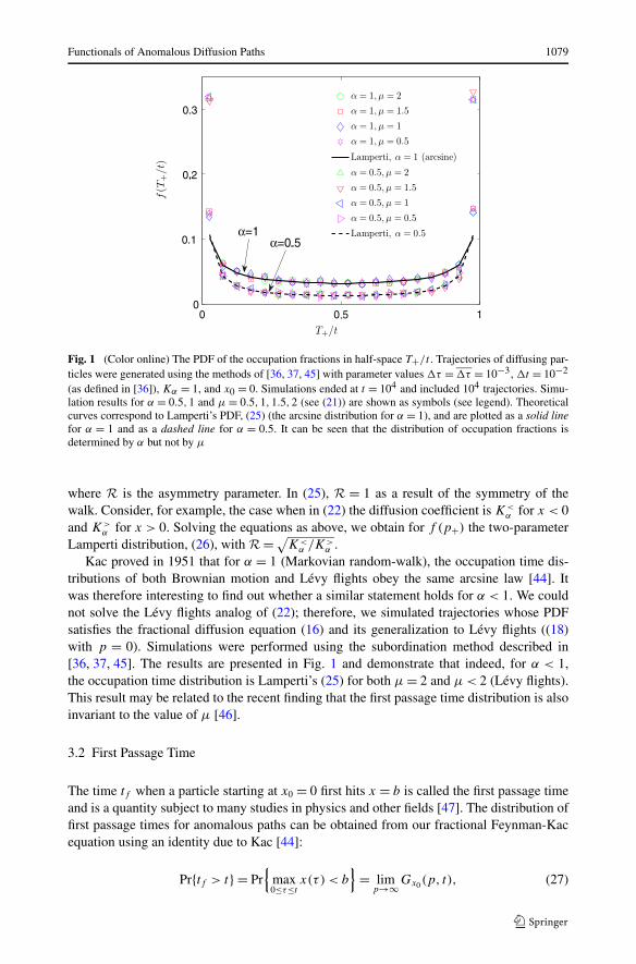
Fig. 1 (Color online) The PDF of the occupation fractions in half-space T+/t . Trajectories of diffusing par-ticles were generated using the methods of [36, 37, 45] with parameter values �τ = �τ = 10−3, �t = 10−2

(as defined in [36]), Kα = 1, and x0 = 0. Simulations ended at t = 104 and included 104 trajectories. Simu-lation results for α = 0.5,1 and μ = 0.5,1,1.5,2 (see (21)) are shown as symbols (see legend). Theoreticalcurves correspond to Lamperti’s PDF, (25) (the arcsine distribution for α = 1), and are plotted as a solid linefor α = 1 and as a dashed line for α = 0.5. It can be seen that the distribution of occupation fractions isdetermined by α but not by μ

where R is the asymmetry parameter. In (25), R = 1 as a result of the symmetry of thewalk. Consider, for example, the case when in (22) the diffusion coefficient is K<

α for x < 0and K>

α for x > 0. Solving the equations as above, we obtain for f (p+) the two-parameterLamperti distribution, (26), with R =√K<

α /K>α .

Kac proved in 1951 that for α = 1 (Markovian random-walk), the occupation time dis-tributions of both Brownian motion and Lévy flights obey the same arcsine law [44]. Itwas therefore interesting to find out whether a similar statement holds for α < 1. We couldnot solve the Lévy flights analog of (22); therefore, we simulated trajectories whose PDFsatisfies the fractional diffusion equation (16) and its generalization to Lévy flights ((18)with p = 0). Simulations were performed using the subordination method described in[36, 37, 45]. The results are presented in Fig. 1 and demonstrate that indeed, for α < 1,the occupation time distribution is Lamperti’s (25) for both μ = 2 and μ < 2 (Lévy flights).This result may be related to the recent finding that the first passage time distribution is alsoinvariant to the value of μ [46].

3.2 First Passage Time

The time tf when a particle starting at x0 = 0 first hits x = b is called the first passage timeand is a quantity subject to many studies in physics and other fields [47]. The distribution offirst passage times for anomalous paths can be obtained from our fractional Feynman-Kacequation using an identity due to Kac [44]:

Pr{tf > t} = Pr{

max0≤τ≤t

x(τ ) < b}

= limp→∞Gx0(p, t), (27)


where the functional is Af = ∫ t

0 U [x(τ)]dτ , and

U(x) ={

0 x < b,

1 x > b.(28)

This is true since Gx0(p, t) = ∫∞0 e−pAf Gx0(Af , t)dAf , and thus, if the particle has never

crossed x = b, we have Af = 0 and e−pAf = 1, while otherwise, Af > 0 and for p → ∞,e−pAf = 0. To find Gx0(p, t) we solve the following backward equation

sGx0(p, s) − 1 =⎧⎨

⎩

Kαs1−α ∂2

∂x20Gx0(p, s) x0 < b,

Kα(s + p)1−α ∂2

∂x20Gx0(p, s) − pGx0(p, s) x0 > b.

Solving these equations as in the previous subsection, demanding that Gx0(p, s) is finite for|x0| → ∞ and demanding continuity of Gx0(p, s) and its first derivative at x0 = b, we obtainfor x0 = 0

G0(p, s) = 1

s

[

1 − e− b√

Kαsα/2 p(s + p)α/2−1

sα/2 + (s + p)α/2

]

.

To find the first passage time distribution we take the limit of infinite p,

limp→∞G0(p, s) = 1

s

(

1 − e− b√

Kαsα/2)

. (29)

Defining τf = (b2/Kα)1/α , we invert s → t :

limp→∞G0(p, t) = Pr{tf > t} = 1 −

∫ t

0

1

τf

lα/2

(τ

τf

)

dτ,

where lα/2(t) is the one-sided Lévy distribution of order α/2, whose Laplace transform is

lα/2(s) = e−sα/2. The PDF of the first passage times, f (t), satisfies f (t) = ∂

∂t(Pr{tf < t}) =

∂∂t

(1 − Pr{tf > t}). Thus,

f (t) = 1

τf

lα/2

(t

τf

)

. (30)

This result has been previously derived using different methods (e.g., equation (53) of [48]).The long times behavior of f (t) is obtained from the s → 0 limit:

f (s) ∼ 1 − b√Kα

sα/2.

Therefore, for long times

f (t) ∼ b∣∣(− α

2

)∣∣√Kα

t−(1+α/2). (31)

For α = 1, we reproduce the famous t−3/2 decay law of a one-dimensional random walk [47].


3.3 The Maximal Displacement

The maximal displacement of a diffusing particle is a random variable whose study hasbeen of recent interest (see, e.g., [49–52] and references therein). To obtain the distributionof this variable, we use the functional defined in the previous subsection (28). Let xm ≡max0≤τ≤t x(τ ), and recall from (27) that Pr{xm < b} = limp→∞ Gx0(p, t). From the previoussubsection we have, for x0 = 0 (29)

Pr{xm < b} = 1

s

(1 − e

− b√Kα

sα/2).

Hence, the PDF of xm is

P (xm, s) = sα/2−1

√Kα

e− xm√

Kαsα/2

.

Inverting s → t , we obtain

P (xm, t) = 2

α√

Kα

t

(xm/√

Kα)1+2/αlα/2

[t

(xm/√

Kα)2/α

]

; xm > 0. (32)

This PDF has the same shape as the PDF of x up to a scale factor of 2 [30], and it is inagreement with the very recent result of [51], derived using a renormalization group method.

3.4 The Hitting Probability

The probability QL(x0) of a particle starting at 0 < x0 < L to hit L before hitting 0 iscalled the hitting (or exit) probability. The hitting probability has been investigated longtime ago for Brownian particles [47] and more recently for some anomalous processes [53].For CTRW, it can be calculated using the following functional:

U(x) ={

0 0 < x < L,

∞ otherwise.(33)

With (33), A = ∫ t

0 U [x(τ)]dτ = 0 as long as the particle did not leave the interval [0,L] andis otherwise infinite. Therefore, G(x,p, t) = ∫∞

0 e−pAG(x,A, t)dA represents the probabil-ity of the particle to be at x at time t without ever leaving [0,L]. This is true for all p, sincee−pA is either 0 or 1 regardless of p. At the boundaries, G(x = 0,p, t) = G(x = L,p, t)

= 0. At (0,L), the forward fractional Feynman-Kac equation (15) reads, in s space,

sG(x, s) − δ(x − x0) = Kαs1−α ∂2

∂x2G(x, s). (34)

Note that (34) does not depend on p and is equivalent to the fractional diffusion equa-tion, (16), with absorbing boundary conditions. The solution of (34) for x = x0 is

G(x, s) =⎧⎨

⎩

C0 sinh[

sα/2√Kα

x]

x < x0,

C1 sinh[

sα/2√Kα

(L − x)]

x > x0.


Matching the solution at x = x0 and demanding ∂∂x

G(x = x+0 , s) − ∂

∂xG(x = x−

0 , s) =− 1

Kαs1−α (from (34)), we have, for x > x0,

G(x, s) = 1√Kαs1−α/2

sinh(

sα/2√Kα

x0

)

sinh(

sα/2√Kα

L) sinh

[sα/2

√Kα

(L − x)

]

; x > x0. (35)

The flux of particles that have never before left [0,L] and that are leaving [0,L] at time t

through the right boundary is [54]

J (L, t) = −Kα D1−αRL,t

∂

∂xG(x = L, t),

where D1−αRL,t is the Riemann-Liouville fractional derivative, equal to s1−α in Laplace t → s

space (see (16)). The hitting probability is the sum over all times of the flux through L [47]:

QL(x0) =∫ ∞

0J (L, t)dt = −Kαs

1−α ∂

∂xG(x = L, s)

∣∣∣∣s=0

.

Using (35), we have

QL(x0) = x0

L. (36)

The hitting probability for anomalous diffusion, α < 1, is the same as in the Browniancase [47]. This is expected, since the hitting probability should not depend on the waitingtime PDF ψ(τ).

Note that a backward equation for QL(x0) can be obtained by the much simpler argumentthat for unbiased CTRW on a lattice, QL(x0) = [QL(x0 + a) + QL(x0 − a)]/2. In the con-

tinuum limit, a → 0, this gives ∂2QL(x0)

∂x20

= 0. With the boundary conditions QL(x0 = 0) = 0

and QL(x0 = L) = 1, (36) immediately follows (see [47] for a binomial random walk).

3.5 The Time in an Interval

Consider the time-in-interval functional Ti = ∫ t

0 U [x(τ)]dτ , where

U(x) ={

1 |x| < b,

0 |x| > b.(37)

Namely, Ti is the total residence time of the particle in the interval [−b, b]. Denote byGx0(Ti, t) the PDF of Ti at time t when the process starts at x0, and denote by Gx0(p, s) theLaplace transform Ti → p, t → s of Gx0(Ti, t). Gx0(p, s) satisfies the backward fractionalFeynman-Kac equation:

sGx0(p, s) − 1 =⎧⎨

⎩

Kα (s + p)1−α ∂2

∂x20Gx0(p, s) − pGx0(p, s) |x0| < b,

Kαs1−α ∂2

∂x20Gx0(p, s) |x0| > b.

(38)

We solve this equation demanding that the solution is finite for |x0| → ∞,

Gx0(p, s) ={

C1 cosh[x0(s + p)α/2/√

Kα] + 1s+p

|x0| < b,

C0 exp[−|x0|sα/2/√

Kα] + 1s

|x0| > b.(39)


Demanding continuity of Gx0(p, s) and its first derivative at x0 = b we solve for C1 and thenobtain for x0 = 0

G0(p, s) =p + s{cosh[

(s+p)α/2√Kα

b]+ (s+p)α/2

sα/2 sinh[

(s+p)α/2√Kα

b]}

s(s + p){cosh[

(s+p)α/2√Kα

b]+ (s+p)α/2

sα/2 sinh[

(s+p)α/2√Kα

b]} . (40)

In principle, the PDF G0(Ti, t) can be obtained from (40) by inverse Laplace transformingp → Ti and s → t . However, we could invert (40) only for α → 0:

G0(Ti, t)α→0 = (1 − e−b/√

K0)δ(Ti − t) + e−b/√

K0δ(Ti). (41)

This can be intuitively explained as follows. For α → 0, the PDF of x becomes time-independent and approaches G(x, t) ≈ exp(−|x|/√K0)/(2

√K0) (equation (A1) in [30]).

With probability∫ b

−bG(x, t)dx = 1 − e−b/

√K0 , the particle never leaves the region [−b, b]

and thus Ti = t ; with probability e−b/√

K0 , the particle is almost never at [−b, b] and thusTi = 0.

The first two moments of Ti can be obtained from (40) by

〈Ti〉(s) = − ∂

∂pG0(p, s)

∣∣∣∣p=0

; 〈T 2i 〉(s) = ∂2

∂p2G0(p, s)

∣∣∣∣p=0

.

Calculating the derivatives, substituting p = 0, and inverting, we obtain, in the long timeslimit,

〈Ti〉 ∼ t1−α/2 b√Kα(2 − α/2)

,

〈T 2i 〉 ∼ t2−α/2 2b(1 − α)√

Kα(3 − α/2)+ t2−α b2(3α − 1)

Kα(3 − α).

(42)

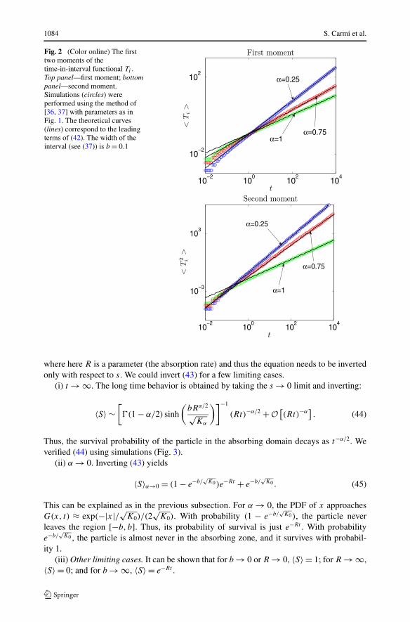
We verified that (42) agrees with simulations (Fig. 2). The average time at [−b, b] scalesas t1−α/2 since this is the product of the average number of returns to the interval [−b, b](∼ tα/2) and the average time spent at [−b, b] on each visit (∼ t1−α ; see equation (61) in[16]). We also see that for α < 1, the PDF of Ti cannot have a scaling form since 〈T 2

i 〉 ∼t2−α/2

� 〈Ti〉2 ∼ t2−α . For α = 1, 〈Ti〉 ∼ t1/2 and 〈T 2i 〉 ∼ t .

3.6 Survival in a Medium with an Absorbing Interval

A problem related to that of the previous subsection is a medium in which a diffusing par-ticle is absorbed at rate R whenever it is in the interval [−b, b]. The survival probabilityof the particle, S, is related to Ti , the total time at [−b, b], through S = exp(−RTi). Thus,if Gx0(Ti, t) is the PDF of Ti at time t , then the Ti → R Laplace transform Gx0(R, t) =∫∞

0 e−RTi Gx0(Ti, t)dTi equals 〈S〉, the survival probability averaged over all trajectories[21]. From (40) of the previous subsection we immediately obtain (in Laplace t → s spaceand for x0 = 0)

〈S〉 = G0(R, s) =R + s{cosh[

(s+R)α/2√Kα

b]+ (s+R)α/2

sα/2 sinh[

(s+R)α/2√Kα

b]}

s(s + R){cosh[

(s+R)α/2√Kα

b]+ (s+R)α/2

sα/2 sinh[

(s+R)α/2√Kα

b]} , (43)


Fig. 2 (Color online) The firsttwo moments of thetime-in-interval functional Ti .Top panel—first moment; bottompanel—second moment.Simulations (circles) wereperformed using the method of[36, 37] with parameters as inFig. 1. The theoretical curves(lines) correspond to the leadingterms of (42). The width of theinterval (see (37)) is b = 0.1

where here R is a parameter (the absorption rate) and thus the equation needs to be invertedonly with respect to s. We could invert (43) for a few limiting cases.

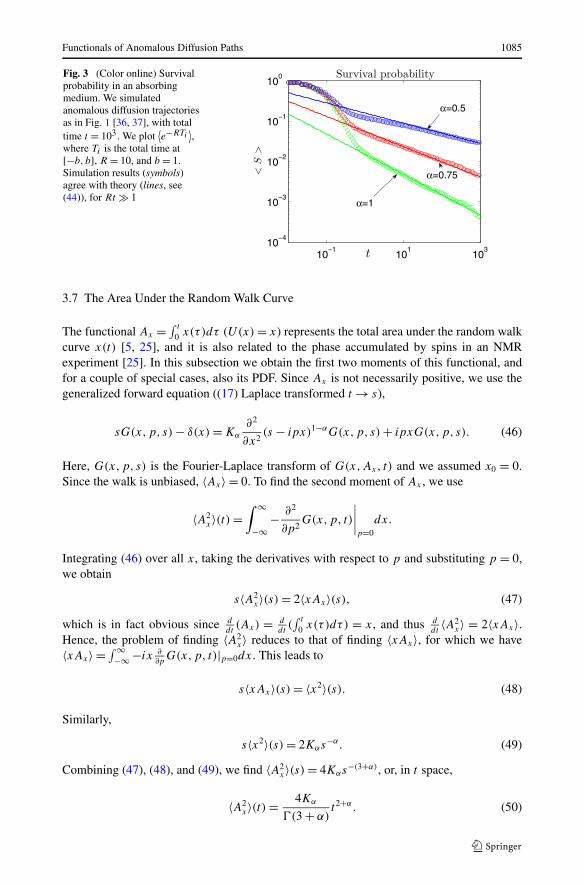
(i) t → ∞. The long time behavior is obtained by taking the s → 0 limit and inverting:

〈S〉 ∼[

(1 − α/2) sinh

(bRα/2

√Kα

)]−1

(Rt)−α/2 + O[(Rt)−α

]. (44)

Thus, the survival probability of the particle in the absorbing domain decays as t−α/2. Weverified (44) using simulations (Fig. 3).

(ii) α → 0. Inverting (43) yields

〈S〉α→0 = (1 − e−b/√

K0)e−Rt + e−b/√

K0 . (45)

This can be explained as in the previous subsection. For α → 0, the PDF of x approachesG(x, t) ≈ exp(−|x|/√K0)/(2

√K0). With probability (1 − e−b/

√K0), the particle never

leaves the region [−b, b]. Thus, its probability of survival is just e−Rt . With probabilitye−b/

√K0 , the particle is almost never in the absorbing zone, and it survives with probabil-

ity 1.(iii) Other limiting cases. It can be shown that for b → 0 or R → 0, 〈S〉 = 1; for R → ∞,

〈S〉 = 0; and for b → ∞, 〈S〉 = e−Rt .


Fig. 3 (Color online) Survivalprobability in an absorbingmedium. We simulatedanomalous diffusion trajectoriesas in Fig. 1 [36, 37], with totaltime t = 103. We plot

⟨e−RTi

⟩,

where Ti is the total time at[−b, b], R = 10, and b = 1.Simulation results (symbols)agree with theory (lines, see(44)), for Rt � 1

3.7 The Area Under the Random Walk Curve

The functional Ax = ∫ t

0 x(τ)dτ (U(x) = x) represents the total area under the random walkcurve x(t) [5, 25], and it is also related to the phase accumulated by spins in an NMRexperiment [25]. In this subsection we obtain the first two moments of this functional, andfor a couple of special cases, also its PDF. Since Ax is not necessarily positive, we use thegeneralized forward equation ((17) Laplace transformed t → s),

sG(x,p, s) − δ(x) = Kα

∂2

∂x2(s − ipx)1−αG(x,p, s) + ipxG(x,p, s). (46)

Here, G(x,p, s) is the Fourier-Laplace transform of G(x,Ax, t) and we assumed x0 = 0.Since the walk is unbiased, 〈Ax〉 = 0. To find the second moment of Ax , we use

〈A2x〉(t) =

∫ ∞

−∞− ∂2

∂p2G(x,p, t)

∣∣∣∣p=0

dx.

Integrating (46) over all x, taking the derivatives with respect to p and substituting p = 0,we obtain

s〈A2x〉(s) = 2〈xAx〉(s), (47)

which is in fact obvious since ddt

(Ax) = ddt

(∫ t

0 x(τ)dτ) = x, and thus ddt

〈A2x〉 = 2〈xAx〉.

Hence, the problem of finding 〈A2x〉 reduces to that of finding 〈xAx〉, for which we have

〈xAx〉 = ∫∞−∞ −ix ∂

∂pG(x,p, t)|p=0dx. This leads to

s〈xAx〉(s) = 〈x2〉(s). (48)

Similarly,

s〈x2〉(s) = 2Kαs−α. (49)

Combining (47), (48), and (49), we find 〈A2x〉(s) = 4Kαs

−(3+α), or, in t space,

〈A2x〉(t) = 4Kα

(3 + α)t2+α. (50)


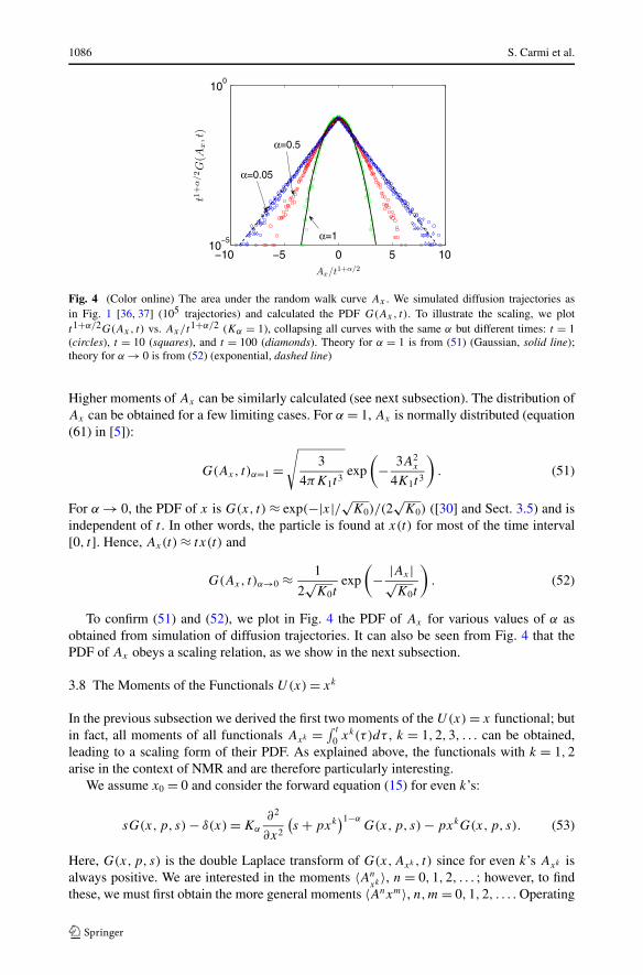
Fig. 4 (Color online) The area under the random walk curve Ax . We simulated diffusion trajectories asin Fig. 1 [36, 37] (105 trajectories) and calculated the PDF G(Ax, t). To illustrate the scaling, we plott1+α/2G(Ax, t) vs. Ax/t1+α/2 (Kα = 1), collapsing all curves with the same α but different times: t = 1(circles), t = 10 (squares), and t = 100 (diamonds). Theory for α = 1 is from (51) (Gaussian, solid line);theory for α → 0 is from (52) (exponential, dashed line)

Higher moments of Ax can be similarly calculated (see next subsection). The distribution ofAx can be obtained for a few limiting cases. For α = 1, Ax is normally distributed (equation(61) in [5]):

G(Ax, t)α=1 =√

3

4πK1t3exp

(

− 3A2x

4K1t3

)

. (51)

For α → 0, the PDF of x is G(x, t) ≈ exp(−|x|/√K0)/(2√

K0) ([30] and Sect. 3.5) and isindependent of t . In other words, the particle is found at x(t) for most of the time interval[0, t]. Hence, Ax(t) ≈ tx(t) and

G(Ax, t)α→0 ≈ 1

2√

K0texp

(

− |Ax |√K0t

)

. (52)

To confirm (51) and (52), we plot in Fig. 4 the PDF of Ax for various values of α asobtained from simulation of diffusion trajectories. It can also be seen from Fig. 4 that thePDF of Ax obeys a scaling relation, as we show in the next subsection.

3.8 The Moments of the Functionals U(x) = xk

In the previous subsection we derived the first two moments of the U(x) = x functional; butin fact, all moments of all functionals Axk = ∫ t

0 xk(τ )dτ , k = 1,2,3, . . . can be obtained,leading to a scaling form of their PDF. As explained above, the functionals with k = 1,2arise in the context of NMR and are therefore particularly interesting.

We assume x0 = 0 and consider the forward equation (15) for even k’s:

sG(x,p, s) − δ(x) = Kα

∂2

∂x2

(s + pxk

)1−αG(x,p, s) − pxkG(x,p, s). (53)

Here, G(x,p, s) is the double Laplace transform of G(x,Axk , t) since for even k’s Axk isalways positive. We are interested in the moments 〈An

xk 〉, n = 0,1,2, . . . ; however, to findthese, we must first obtain the more general moments 〈Anxm〉, n,m = 0,1,2, . . . . Operating


on each term of (53) with (−1)n ∂n

∂pn , substituting p = 0, multiplying each term by xm, andintegrating over all x, (53) becomes

s〈Anxm〉(s) = δn,0δm,0 + Hn−1n〈An−1xm+k〉(s)

+ Hm−2Kαm(m − 1)

n∑

j=0

(n

j

)[j−1∏

l=0

(1 − α − l)

]

(−1)j s1−α−j

× 〈An−j xm+jk−2〉(s), (54)

where δi,j is Kronecker’s delta function—δi,j equals 1 for i = j and equals zero otherwise;and Hi is the discrete Heaviside function—Hi equals 1 for i ≥ 0 and equals zero otherwise.It can be proved that (54) remains true also for odd k’s, when Axk can be either positive ornegative. Equation (54) is satisfied by the following choice of 〈Anxm〉:

〈Anxm〉(s) = cn,m(k)Km+nk

2α s−(1+n+ m+nk

2 α), (55)

for all n and even m when k is even and for even (n + m) when k is odd. In all othercases 〈Anxm〉 = 0 due to symmetry. The cn,m’s are k-dependent dimensionless constantsthat satisfy the following recursion equation:

cn,m(k) = δn,0δm,0 + Hn−1ncn−1,m+k(k)

+ Hm−2m(m − 1)

n∑

j=0

(n

j

)[j−1∏

l=0

(1 − α − l)

]

(−1)j cn−j,m+jk−2(k), (56)

with initial conditions c0,0(k) = 1 and c0,1(k) = 0. The moments of Axk are therefore givenin t space by

〈An

xk 〉(t) = cn,0(k)K

nk2

α

(1 + n + nαk

2

) tn(1+ αk2 ). (57)

For example, for k = 1, 〈Ax〉 = 〈A3x〉 = 0, 〈A2

x〉 = 4Kαt2+α/(3 + α) (50), and 〈A4

x〉 =48(α2 + 7α + 12)K2

αt4+2α/(5 + 2α); while for k = 2, 〈Ax2〉 = 2Kαt1+α/(2 + α) and

〈A2x2〉 = (48 + 8α)K2

αt2+2α/(3 + 2α).Equation (57) suggests that the PDF of Axk obeys the scaling relation

G(Axk , t) = 1

Kk/2α t1+αk/2

gα,k

(Axk

Kk/2α t1+αk/2

)

, (58)

where gα,k(x) is a dimensionless scaling function. To verify the scaling form of (58), weplot in Fig. 4 simulation results for the PDF of Ax (k = 1) for α ≈ 0 and α = 1 (for whichG(Ax, t) is known—(51) and (52) in the previous subsection), and for an intermediate value,α = 0.5. In all cases the simulated PDF satisfies the scaling form (58).

4 Summary and Discussion

Functionals of the path of a Brownian particle have been investigated in numerous studiessince the development of the Feynman-Kac equation in 1949. However, an analog equation


for functionals of non-Brownian particles has been missing. Here, we developed such anequation based on the CTRW model with broadly distributed waiting times. We derivedforward and backward equations ((12) and (20)) and generalizations to Lévy flights ((18)and (21)). Using the backward equation, we derived the PDFs of the occupation time inhalf-space, the first passage time, and the maximal displacement, and calculated the averagesurvival probability in an absorbing medium. Using the forward equation, we calculated thehitting probability and all the moments of U(x) = xk functionals.

The fractional Feynman-Kac equation (12) can be obtained from the integer equation (1)by insertion of a substantial fractional derivative operator [28]. In that sense, our work is anatural generalization of that of Kac’s. The distributions we obtained for specific function-als are also the expected extensions of their Brownian counterparts: the arcsine law for theoccupation time in half-space [1, 43] was replaced by Lamperti’s PDF (25) [22], and the fa-mous t−3/2 decay of the one-dimensional first passage time PDF [47] became t−(1+α/2) (31).Thus, our analysis supports the notion that CTRW and the emerging fractional paths [36, 37]are elegant generalizations of ordinary Brownian motion. Nevertheless, other non-Brownianprocesses are also important. For example, it would be interesting to find an equation for thePDF of anomalous functionals when the underlying process is fractional Brownian mo-tion [14].

Our fractional Feynman-Kac equation (12) has the form of a fractional Schrödinger equa-tion in imaginary time. Real time, fractional Schrödinger equations for the wave functionhave also been recently proposed [55–59]. However, these are very different from our frac-tional Feynman-Kac equation. In [55–57], the Laplacian was replaced with a fractional spa-tial derivative which would correspond to a Markovian CTRW with heavy tailed distribu-tion of jump lengths (Lévy flights; see also the Appendix below). The approach in [58, 59]is based on a temporal fractional Riemann-Liouville derivative—however not substantial—which leads to non-Hermitian evolution and hence non-normalizable quantum mechanics.It is unclear yet whether all these fractional Schrödinger equations actually describe anyphysical phenomenon (see [60] for discussion). In principle, a fractional Schrödinger equa-tion can also be written using the substantial fractional derivative we used here. If there is aphysical process behind such a quantum mechanical analog of our equation remains at thisstage unclear.

In this paper we considered only the case of a free particle. In [29], we reported a frac-tional Feynman-Kac equation for a particle under the influence of a binding force, whereanomalous diffusion can lead to weak ergodicity breaking [61–63]. The derivation of anequation for the distribution of general functionals and the treatment of specific functionalsfor bounded particles will be published elsewhere.

Acknowledgements We thank S. Burov for discussions and the Israel Science Foundation for financialsupport. S.C. is supported by the Adams Fellowship Program of the Israel Academy of Sciences and Human-ities.

Appendix: Generalization to Arbitrary Functionals and Lévy Flights

Here we generalize our forward and backward fractional Feynman-Kac equations ((12)and (20), respectively) to the case when the functional is not necessarily positive and to thecase when the CTRW jump length distribution is arbitrary, and in particular, heavy tailed.

In our generalized CTRW model, the particle moves, after waiting at x, to x + �x ,where �x is distributed according to f (�x). The PDF f (�x) must be symmetric: f (�x) =


f (−�x) but can be otherwise arbitrary. Let us rederive the forward equation for this model.We replace (4) with

Qn+1(x,A, t) =∫ t

0ψ(τ)

∫ ∞

−∞f (�x)Qn[x − �x,A − τU(x − �x), t − τ ]d�xdτ.

Since A can be negative, we Fourier transform the last equation A → p

Qn+1(x,p, t) =∫ t

0ψ(τ)

∫ ∞

−∞f (�x)e

ipτU(x−�x)Qn(x − �x,p, t − τ)d�xdτ.

Laplace transforming t → s and Fourier transforming x → k we have

Qn+1(k,p, s) =∫ ∞

−∞eikx

∫ ∞

−∞f (�x)ψ[s − ipU(x − �x)]Qn(x − �x,p, s)d�xdx.

Changing variables: x ′ = x − �x ,

Qn+1(k,p, s) =∫ ∞

−∞eik�x f (�x)d�x

∫ ∞

−∞eikx′

ψ[s − ipU(x ′)]Qn(x′,p, s)dx ′

= f (k)ψ

[

s − ipU

(

−i∂

∂k

)]

Qn(k,p, s).

Summing over all n and using the initial condition Q0(k,p, s) = eikx0 ,

∞∑

n=0

Qn(k,p, s) ={

1 − f (k)ψ

[

s − ipU

(

−i∂

∂k

)]}−1

eikx0 .

Note that this agrees with (8) since for nearest neighbor hopping f (k) = ∫∞−∞ eik�x

[ 12δ(�x − a) + 1

2δ(�x + a)]d�x = cos(ka). Next, we observe that (3) of Sect. 2.1 remainsthe same even under the general conditions. Calculating the transformed G(k,p, s) as above,and using the result of the last equation, we obtain the formal solution

G(k,p, s) = 1 − ψ[s − ipU

(−i ∂∂k

)]

s − ipU(−i ∂

∂k

)

×{

1 − f (k)ψ

[

s − ipU

(

−i∂

∂k

)]}−1

eikx0 .

We now assume that f (�x) has a finite second moment and thus its characteristic functioncan be written, for small k, as f (k) ∼ 1 −σ 2k2/2. This characteristic function is identical tothat of nearest neighbor hopping (with σ = a); we can thus proceed as in Sect. 2.1 to obtain

∂

∂tG(x,p, t) = Kα

∂2

∂x2D1−α

t G(x,p, t) + ipU(x)G(x,p, t), (59)

where here D1−αt → [s − ipU(x)]1−α in Laplace s space and Kα = σ 2/(2Bα).

Consider now the case of Lévy flights—f (�x) ∼ |�x |−(1+μ) (for large �x ) with0 < μ < 2, and thus jump lengths have a diverging second moment. The characteristic func-tion is f (k) ∼ 1 − Cμ|k|μ, and the fractional Feynman-Kac equation becomes

∂

∂tG(x,p, t) = Kα,μ∇μ

x D1−αt G(x,p, t) + ipU(x)G(x,p, t), (60)


where Kα,μ = Cμ/Bα and ∇μx is the Riesz spatial fractional derivative operator: ∇μ

x →−|k|μ in Fourier k space.

Repeating the calculations of Sect. 2.2 for a non-necessarily-positive functional and forLévy flights, it can be shown that the generalized backward equation is:

∂

∂tGx0(p, t) = Kα,μD1−α

t ∇μx0

Gx0(p, t) + ipU(x0)Gx0(p, t). (61)

Here, D1−αt → [s − ipU(x0)]1−α in Laplace s space and ∇μ

x0→ −|k0|μ in Fourier k0 space.

References

1. Majumdar, S.N.: Brownian functionals in physics and computer science. Curr. Sci. 89, 2076 (2005)2. Comtet, A., Desbois, J., Texier, C.: Functionals of Brownian motion, localization and metric graphs.

J. Phys. A: Math. Gen. 38, R341 (2005)3. Foltin, G., Oerding, K., Racz, Z., Workman, R.L., Zia, R.P.K.: Width distribution for random-walk inter-

faces. Phys. Rev. E 50, R639 (1994)4. Hummer, G., Szabo, A.: Free energy reconstruction from nonequilibrium single-molecule pulling exper-

iments. Proc. Natl. Acad. Sci. USA 98, 3658 (2001)5. Baule, A., Friedrich, R.: Investigation of a generalized Obukhov model for turbulence. Phys. Lett. A 350,

167 (2006)6. Majumdar, S.N., Bray, A.J.: Large-deviation functions for nonlinear functionals of a Gaussian stationary

Markov process. Phys. Rev. E 65, 051112 (2002)7. Comtet, A., Monthus, C., Yor, M.: Exponential functionals of Brownian motion and disordered systems.

J. Appl. Probab. 35, 255 (1998)8. Yor, M.: On Exponential Functionals of Brownian Motion and Related Processes. Springer, Berlin

(2001)9. Kac, M.: On distributions of certain Wiener functionals. Trans. Am. Math. Soc. 65, 1 (1949)

10. Havlin, S., ben-Avraham, D.: Diffusion in disordered media. Adv. Phys. 36, 695 (1987)11. Bouchaud, J.P., Georges, A.: Anomalous diffusion in disordered media: Statistical mechanisms, models

and physical applications. Phys. Rep. 195, 127 (1990)12. Metzler, R., Klafter, J.: The random walks’s guide to anomalous diffusion: A fractional dynamics ap-

proach. Phys. Rep. 339, 1 (2000)13. Klages, R., Radons, G., Sokolov, I.M. (eds.): Anomalous Transport: Foundations and Applications. Wi-

ley, Weinheim (2008)14. Mandelbrot, B.B., Van Ness, J.W.: Fractional Brownian motions, fractional noises and applications.

SIAM Rev. 10, 422 (1968)15. Majumdar, S.N., Comtet, A.: Local and occupation time of a particle diffusing in a random medium.

Phys. Rev. Lett. 89, 060601 (2002)16. Barkai, E.: Residence time statistics for normal and fractional diffusion in a force field. J. Stat. Phys.

123, 883 (2006)17. Gandjbakhche, A.H., Weiss, G.H.: Descriptive parameter for photon trajectories in a turbid medium.

Phys. Rev. E 61, 6958 (2000)18. Bar-Haim, A., Klafter, J.: On mean residence and first passage times in finite one-dimensional systems.

J. Chem. Phys. 109, 5187 (1998)19. Agmon, N.: Residence times in diffusion processes. J. Chem. Phys. 81, 3644 (1984)20. Agmon, N.: The residence time equation. Chem. Phys. Lett. 497, 184 (2010)21. Grebenkov, D.S.: Residence times and other functionals of reflected Brownian motion. Phys. Rev. E 76,

041139 (2007)22. Lamperti, J.: An occupation time theorem for a class of stochastic processes. Trans. Am. Math. Soc. 88,

380 (1958)23. Sabhapandit, S., Majumdar, S.N., Comtet, A.: Statistical properties of functionals of the paths of a parti-

cle diffusing in a one-dimensional random potential. Phys. Rev. E 73, 051102 (2006)24. Karlin, S., Taylor, H.M.: A Second Course in Stochastic Processes. Academic Press, New York (1981)25. Grebenkov, D.S.: NMR survey of reflected Brownian motion. Rev. Mod. Phys. 79, 1077 (2007)26. Montroll, E.W., Weiss, G.H.: Random walks on lattices. II. J. Math. Phys. 6, 167 (1965)27. Scher, H., Montroll, E.: Anomalous transit-time dispersion in amorphous solids. Phys. Rev. B 12, 2455

(1975)


28. Friedrich, R., Jenko, F., Baule, A., Eule, S.: Anomalous diffusion of inertial, weakly damped particles.Phys. Rev. Lett. 96, 230601 (2006)

29. Turgeman, L., Carmi, S., Barkai, E.: Fractional Feynman-Kac equation for non-Brownian functionals.Phys. Rev. Lett. 103, 190201 (2009)

30. Barkai, E., Metzler, R., Klafter, J.: From continuous time random walks to the fractional Fokker-Planckequation. Phys. Rev. E 61, 132 (2000)

31. Meerschaert, M.M., Scheffler, H.P.: Limit theorems for continuous-time random walks with infinite meanwaiting times. J. Appl. Probab. 41, 623 (2004)

32. Kotulski, M.: Asymptotic distributions of continuous-time random walks: A probabilistic approach.J. Stat. Phys. 81, 777 (1995)

33. Weissman, H., Weiss, G.H., Havlin, S.: Transport properties of the continuous-time random walk with along-tailed waiting-time density. J. Stat. Phys. 57, 301 (1989)

34. Schneider, W.R., Wyss, W.: Fractional diffusion and wave equations. J. Math. Phys. 30, 134 (1988)35. Fogedby, H.C.: Langevin equations for continuous time Lévy flights. Phys. Rev. E 50, 1657 (1994)36. Magdziarz, M., Weron, A., Weron, K.: Fractional Fokker-Planck dynamics: Stochastic representation

and computer simulation. Phys. Rev. E 75, 016708 (2007)37. Kleinhans, D., Friedrich, R.: Continuous-time random walks: Simulation of continuous trajectories.

Phys. Rev. E 76, 061102 (2007)38. Godrèche, C., Luck, J.M.: Statistics of the occupation time of renewal processes. J. Stat. Phys. 104, 489

(2001)39. Baldassarri, A., Bouchaud, J.P., Dornic, I., Godrèche, C.: Statistics of persistent events: an exactly soluble

model. Phys. Rev. E 59, 20 (1999)40. Margolin, G., Barkai, E.: Non-ergodicity of blinking nano crystals and other Lévy walk processes. Phys.

Rev. Lett. 94, 080601 (2005)41. Margolin, G., Barkai, E.: Non-ergodicity of a time series obeying Lévy statistics. J. Stat. Phys. 122, 137

(2006)42. Stefani, F.D., Hoogenboom, J.P., Barkai, E.: Beyond quantum jumps: Blinking nano-scale light emitters.

Phys. Today 62, 34 (2009)43. Watanabe, S.: Generalized arc-sine laws for one-dimensional diffusion processes and random walks.

Proc. Symp. Pure Math. 57, 157 (1995)44. Kac, M.: On some connections between probability theory and differential and integral equations. In:

Second Berkeley Symposium on Mathematical Statistics and Probability, Berkeley, CA, USA, p. 189(1951). University of California Press

45. Magdziarz, M., Weron, A.: Competition between subdiffusion and Lévy flights: a Monte Carlo approach.Phys. Rev. E 75, 056702 (2007)

46. Dybiec, B., Gudowska-Nowak, E.: Anomalous diffusion and generalized Sparre Andersen scaling. EPL88, 10003 (2009)

47. Redner, S.: A Guide to First-Passage Processes. Cambridge University Press, Cambridge (2001)48. Barkai, E.: Fractional Fokker-Planck equation, solution, and application. Phys. Rev. E 63, 046118 (2001)49. Comtet, A., Majumdar, S.N.: Precise asymptotics for a random walkers maximum. J. Stat. Mech. P06013

(2005)50. Majumdar, S.N., Randon-Furling, J., Kearney, M.J., Yor, M.: On the time to reach maximum for a variety

of constrained Brownian motions. J. Phys. A, Math. Theor. 41, 365005 (2008)51. Schehr, G., Le-Doussal, P.: Extreme value statistics from the real space renormalization group: Brownian

motion, Bessel processes and continuous time random walks. J. Stat. Mech. P01009 (2010)52. Tejedor, V., Bénichou, O., Voituriez, R., Jungmann, R., Simmel, F., Selhuber-Unkel, C., Oddershede,

L.B., Metzler, R.: Quantitative analysis of single particle trajectories: mean maximal excursion method.Biophys. J. 98, 1364 (2010)

53. Majumdar, S.N., Rosso, A., Zoia, A.: Hitting probability for anomalous diffusion processes. Phys. Rev.Lett. 104, 020602 (2010)

54. Metzler, R., Barkai, E., Klafter, J.: Anomalous diffusion and relaxation close to thermal equilibrium:a fractional Fokker-Planck equation approach. Phys. Rev. Lett. 82, 3563 (1999)

55. Hu, Y., Kallianpur, G.: Schrödinger equations with fractional Laplacians. Appl. Math. Optim. 42, 281(2000)

56. Laskin, N.: Fractional quantum mechanics. Phys. Rev. E 62, 3135 (2000)57. Laskin, N.: Fractional Schrödinger equation. Phys. Rev. E 66, 056108 (2002)58. Naber, M.: Time fractional Schrödinger equation. J. Math. Phys. 45, 3339 (2004)59. Wang, S., Xu, M.: Generalized fractional Schrödinger equation with spacetime fractional derivatives.

J. Math. Phys. 48, 043502 (2007)


60. Iomin, A.: Fractional-time quantum dynamics. Phys. Rev. E 80, 022103 (2009)61. Rebenshtok, A., Barkai, E.: Distribution of time-averaged observables for weak ergodicity breaking.

Phys. Rev. Lett. 99, 210601 (2007)62. Bel, G., Barkai, E.: Weak ergodicity breaking in the continuous-time random walk. Phys. Rev. Lett. 94,

240602 (2005)63. Rebenshtok, A., Barkai, E.: Weakly non-ergodic statistical physics. J. Stat. Phys. 133, 565 (2008)

Documents

On Distributions of Functionals of Anomalous Diffusion Paths