Embed Size (px)
Citation preview
Anomalous Diffusion, Anomalous Time Series, and the models that
describe them.
Nick Watkins NERC British Antarctic Survey
Cambridge, UK [email protected]

Thanks Rainer and the LDSG for the invitation Sandra Chapman, Bogdan Hnat, John Greenhough (Warwick), Mervyn Freeman, Christian Franzke, Sam Rosenberg, Dan Credgington (BAS), Bobby Gramacy and Tim Graves (Cambridge) , and many others.
Summary
Why stochastic models ? Textbook stochastic models Noah, Joseph and volatility bunching A physics of fractals ? From fractals back to physics ? Pitfalls: 1. Walks are not noises 2. Memory not always from self-similarity 3. Choice of fractal models
WHY STOCHASTIC MODELS ?
• We need to use stochastic (or partly stochastic) models in physics and the geosciences, particularly in time series analysis. Partly as models when computational
bandwidth or other issues prevent a fully deterministic model But also as paradigms to help us frame the
right statistical questions about data.

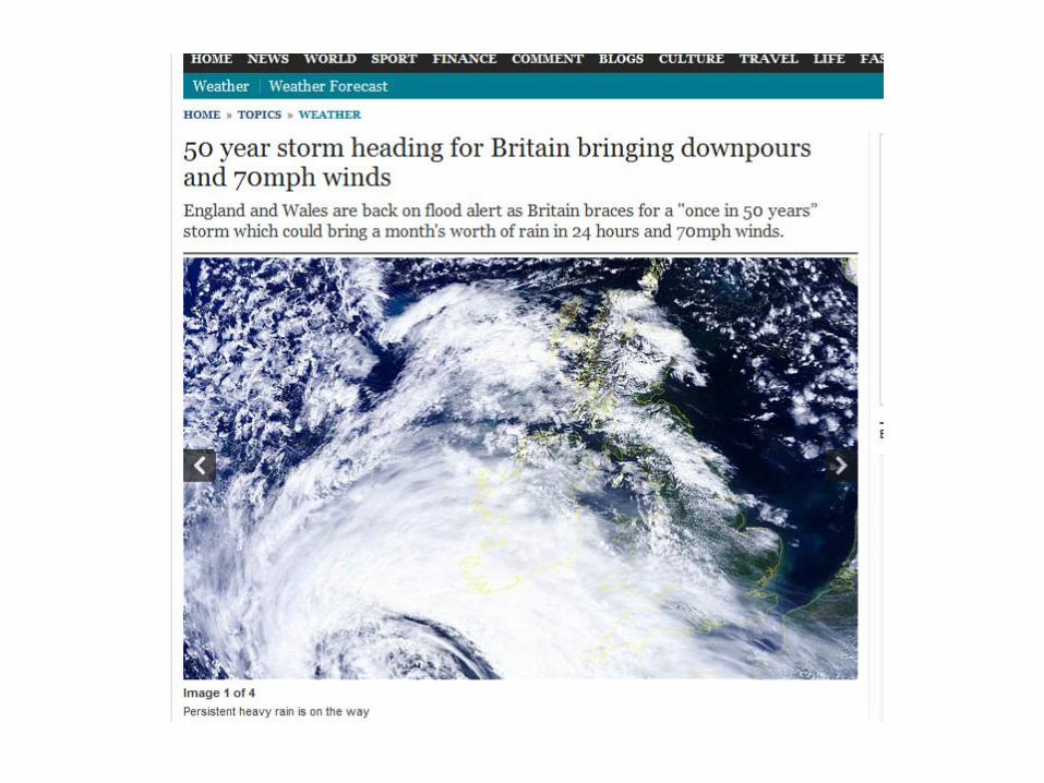
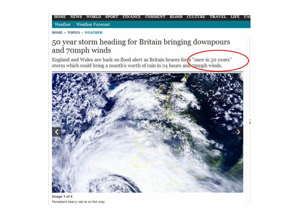
• Motivation not only the classic problems but also increasing importance of topics like extremes and large deviations.
• Couple of examples of relevance to the environmental sciences: Extreme weather events Solar Terrestrial Physics (“Space Weather”)

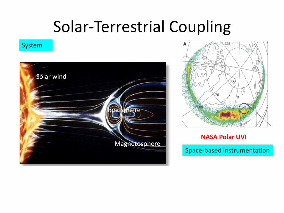
Solar-Terrestrial Coupling
Solar wind
Ionosphere
Magnetosphere
System
Space-based instrumentation
NASA Polar UVI

Convection (DP2)
• Mass, momentum and energy input from reconnection at solar wind - magnetosphere interface.
• Plasma circulation from day to night over poles and from night to day around flanks.
• magnetic pole
equator
Sun
flow
solar wind
magnetosphere
Courtesy Mervyn Freeman
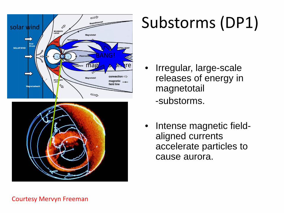
Substorms (DP1)
• Irregular, large-scale releases of energy in magnetotail
-substorms.
• Intense magnetic field-aligned currents accelerate particles to cause aurora.
solar wind
magnetosphere BANG!
Courtesy Mervyn Freeman
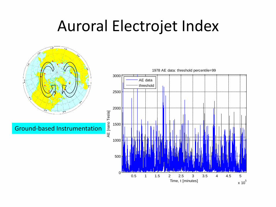
Auroral Electrojet Index
Ionosphere
Magnetosphere
Ground-based Instrumentation
0.5 1 1.5 2 2.5 3 3.5 4 4.5 5
x 105
0
500
1000
1500
2000
2500
30001978 AE data: threshold percentile=99
Time, t [minutes]
AE
[nan
o Te
sla]
AE datathreshold
“TEXTBOOK” STOCHASTIC MODEL
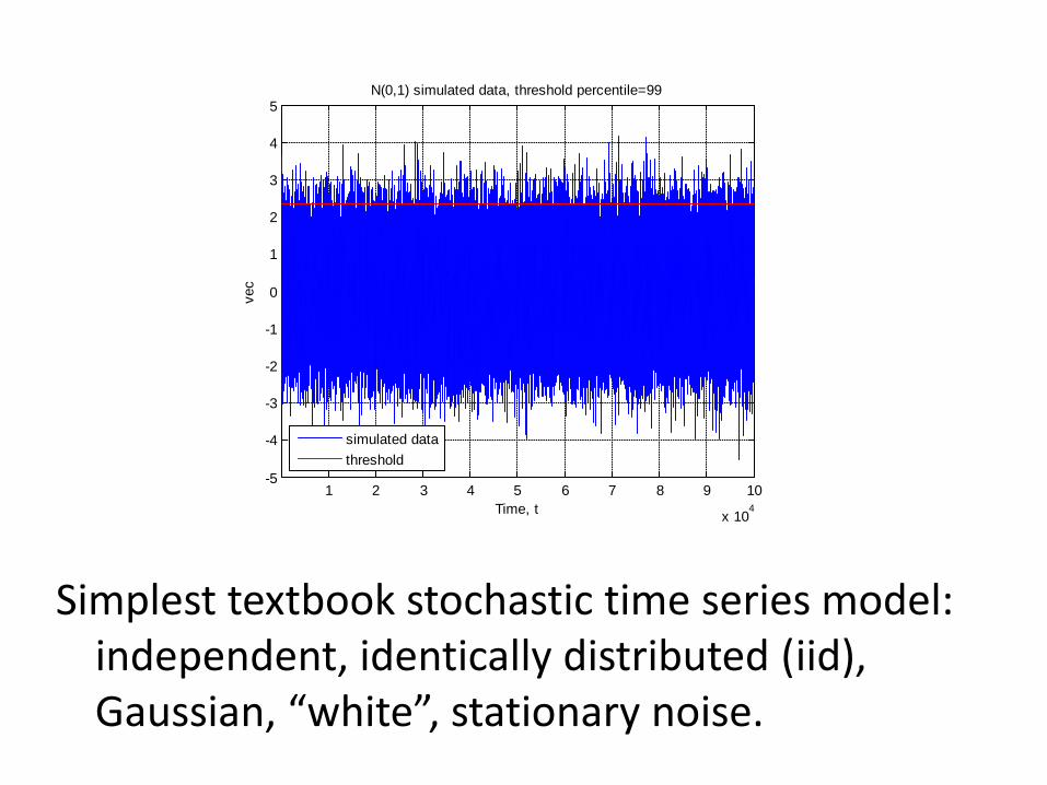
Simplest textbook stochastic time series model: independent, identically distributed (iid), Gaussian, “white”, stationary noise.
1 2 3 4 5 6 7 8 9 10
x 104
-5
-4
-3
-2
-1
0
1
2
3
4
5N(0,1) simulated data, threshold percentile=99
Time, t
vec
simulated datathreshold
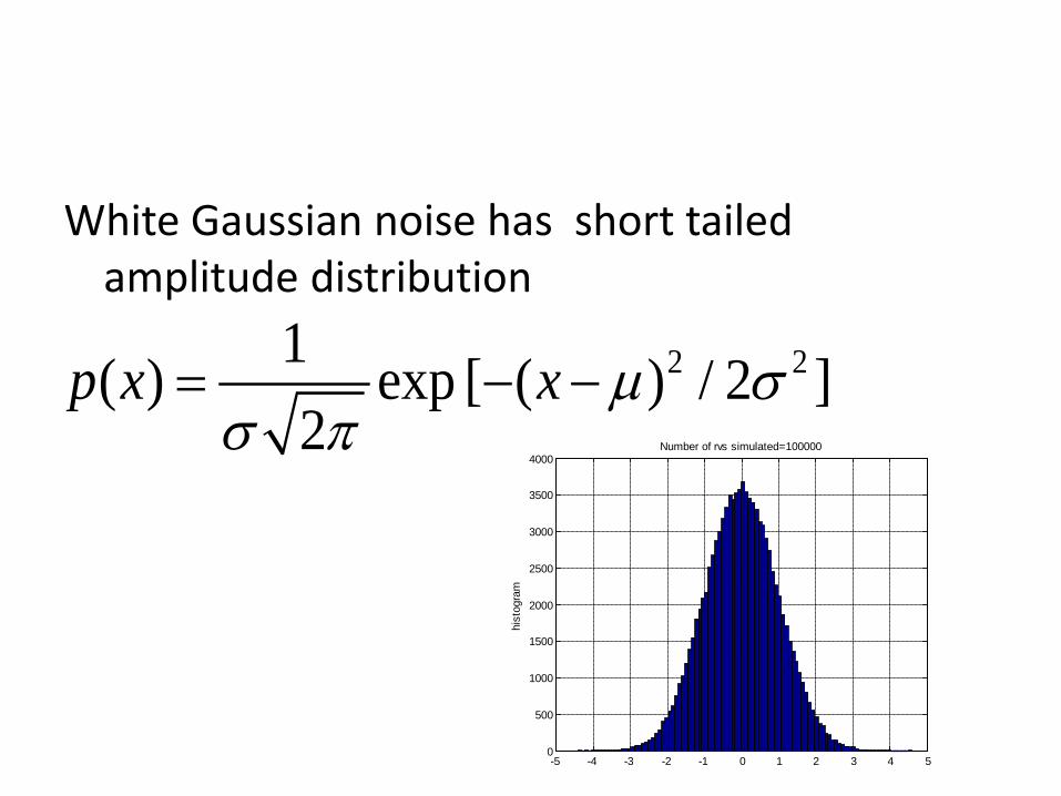
White Gaussian noise has short tailed amplitude distribution
-5 -4 -3 -2 -1 0 1 2 3 4 50
500
1000
1500
2000
2500
3000
3500
4000
hist
ogra
m
Number of rvs simulated=100000
2 21 exp [( / 2 ]) ( )2
xp x µ σσ π
− −=
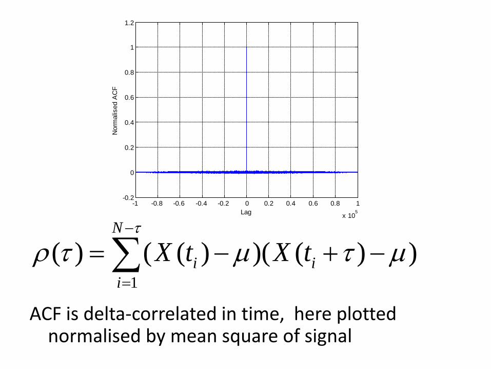
ACF is delta-correlated in time, here plotted
normalised by mean square of signal
1
( ( )( (( ) ) ) )N
i ii
X t X tτ
ρ τ µ τ µ−
=
= − −+∑-1 -0.8 -0.6 -0.4 -0.2 0 0.2 0.4 0.6 0.8 1
x 105
-0.2
0
0.2
0.4
0.6
0.8
1
1.2
Nor
mal
ised
AC
F
Lag
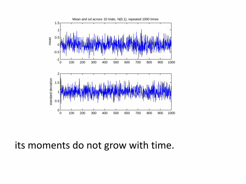
its moments do not grow with time.
0 100 200 300 400 500 600 700 800 900 1000-1
-0.5
0
0.5
1
1.5
mea
n
Mean and sd across 10 trials, N(0,1), repeated 1000 times
0 100 200 300 400 500 600 700 800 900 10000
0.5
1
1.5
2
stan
dard
dev
iatio
n

NOAH, JOSEPH AND VOLATILITY
• In stark contrast, Mandelbrot's classic work in the 1960s and early 1970s focused particularly on 3 “anomalous” effects seen in time series drawn from the natural and economic sciences, each of which represented a strong departure from one of the above properties of white noise.
AE time series exhibits them all to some degree – has forced us to explore beyond simple noise models.
[Have removed some unpublished AE work, paper in preparation]
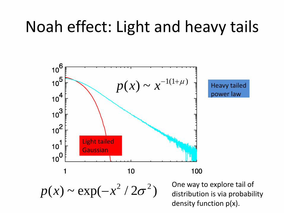
Noah effect: Light and heavy tails
Light tailed Gaussian
Heavy tailed power law
1(1 )( ) ~ xp x µ− +
2 2~ exp(( ) / )2xp x σ− One way to explore tail of distribution is via probability density function p(x).
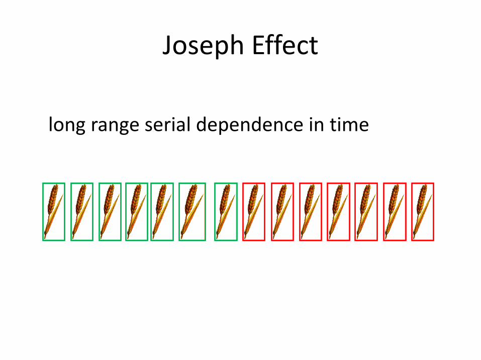
Joseph Effect
long range serial dependence in time
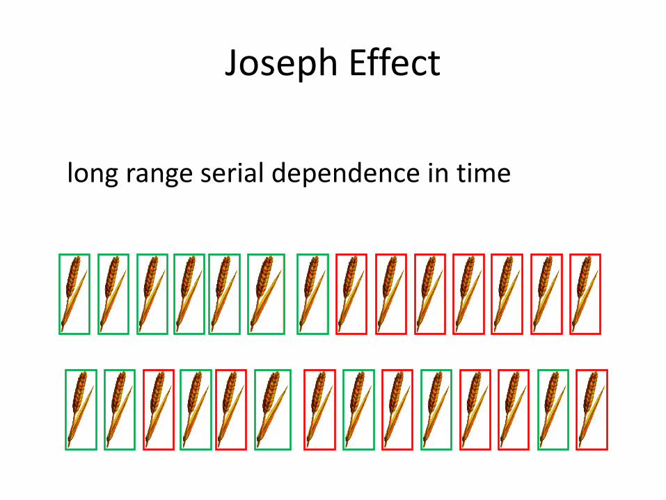
Joseph Effect
long range serial dependence in time
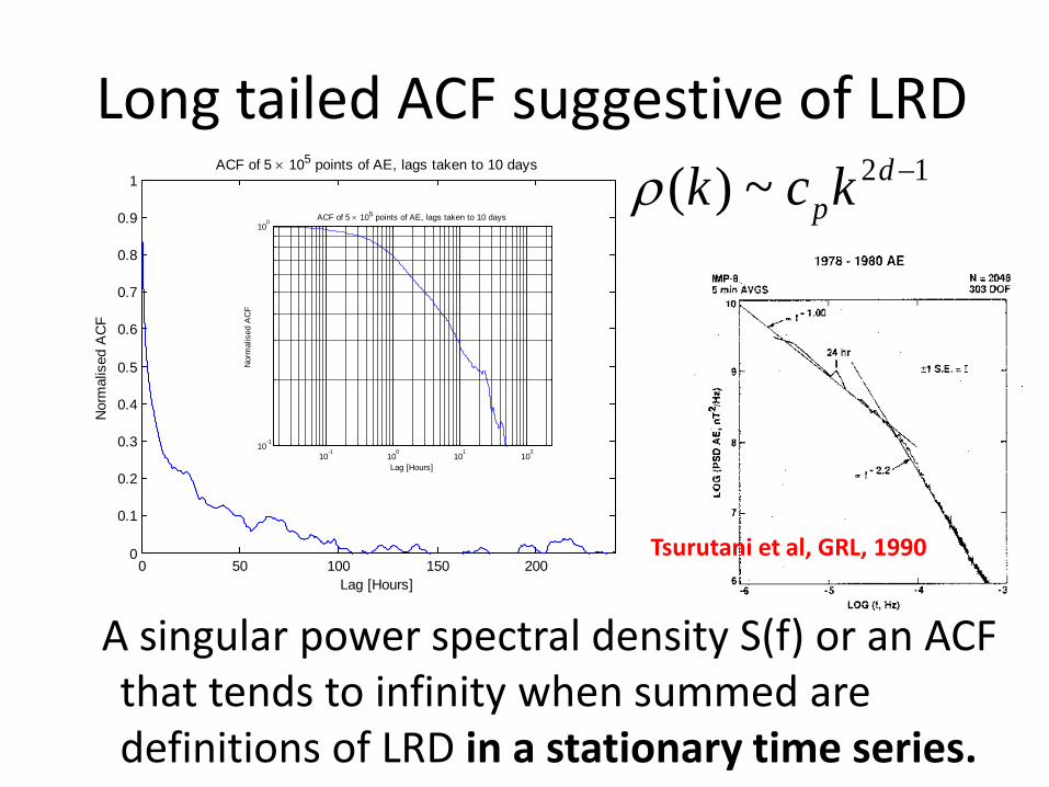
Long tailed ACF suggestive of LRD
A singular power spectral density S(f) or an ACF that tends to infinity when summed are definitions of LRD in a stationary time series.
2 1( ) ~ dpk c kρ −
0 50 100 150 2000
0.1
0.2
0.3
0.4
0.5
0.6
0.7
0.8
0.9
1
Nor
mal
ised
AC
F
Lag [Hours]
ACF of 5 × 10⁵ points of AE, lags taken to 10 days
10-1
100
101
102
10-1
100
Nor
mal
ised
AC
F
Lag [Hours]
ACF of 5 × 10⁵ points of AE, lags taken to 10 days
Tsurutani et al, GRL, 1990
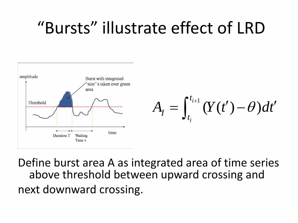
“Bursts” illustrate effect of LRD
Define burst area A as integrated area of time series
above threshold between upward crossing and next downward crossing.
1 ( ( ) )i
i
t
I tA Y t dtθ+ ′ ′= −∫
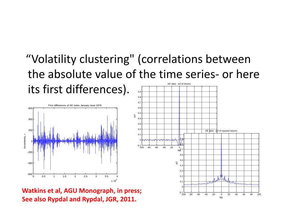
“Volatility clustering" (correlations between the absolute value of the time series- or here its first differences).
0 0.5 1 1.5 2 2.5 3 3.5 4
x 104
-600
-400
-200
0
200
400
600
incr
emen
ts, r
First differences of AE index January-June 1979
-100 -80 -60 -40 -20 0 20 40 60 80 100-0.1
0
0.1
0.2
0.3
0.4
0.5
0.6
0.7
0.8
0.9
lag
acf
AE data: acf of returns
-100 -80 -60 -40 -20 0 20 40 60 80 100-0.1
0
0.1
0.2
0.3
0.4
0.5
0.6
0.7
0.8
0.9
lag
acf
AE data: acf of squared returns
Watkins et al, AGU Monograph, in press; See also Rypdal and Rypdal, JGR, 2011.
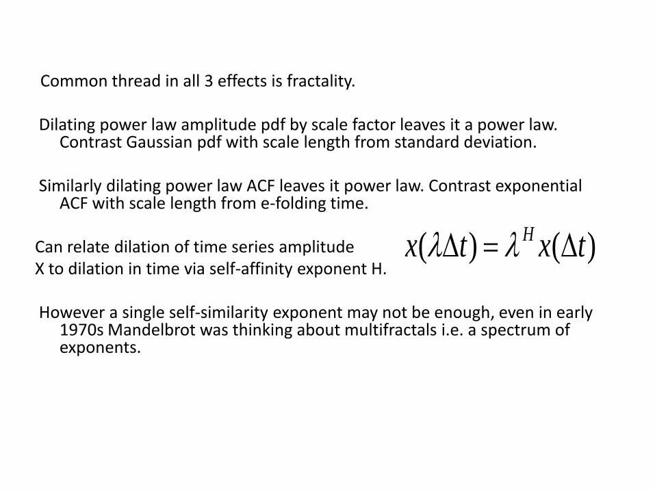
Common thread in all 3 effects is fractality. Dilating power law amplitude pdf by scale factor leaves it a power law.
Contrast Gaussian pdf with scale length from standard deviation. Similarly dilating power law ACF leaves it power law. Contrast exponential
ACF with scale length from e-folding time. Can relate dilation of time series amplitude X to dilation in time via self-affinity exponent H. However a single self-similarity exponent may not be enough, even in early
1970s Mandelbrot was thinking about multifractals i.e. a spectrum of exponents.
) (( )Ht x tx λ λ∆ = ∆
A PHYSICS OF FRACTALS ?

Bak et al’s self-organised criticality, introduced (PRL, 1987; PRE, ‘88) to unify Noah & Joseph effects through self-similar “avalanches”.
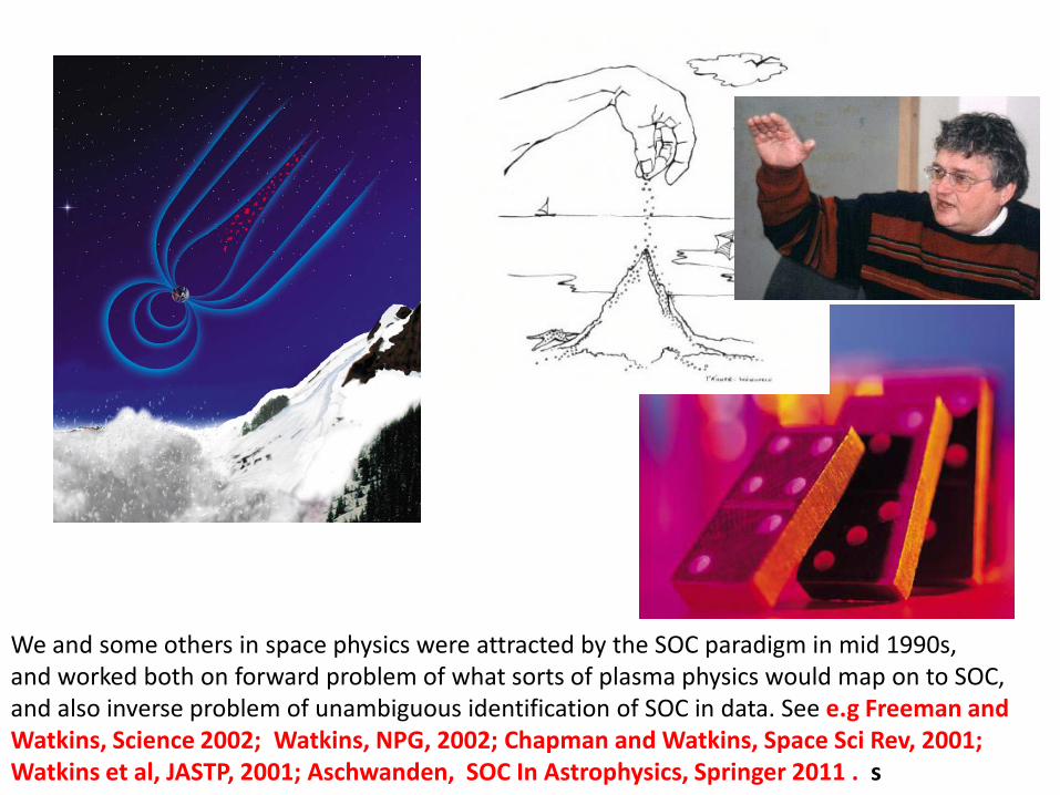
We and some others in space physics were attracted by the SOC paradigm in mid 1990s, and worked both on forward problem of what sorts of plasma physics would map on to SOC, and also inverse problem of unambiguous identification of SOC in data. See e.g Freeman and Watkins, Science 2002; Watkins, NPG, 2002; Chapman and Watkins, Space Sci Rev, 2001; Watkins et al, JASTP, 2001; Aschwanden, SOC In Astrophysics, Springer 2011 . s
FROM FRACTALS TO PHYSICS ?
• Initial interest in extreme fluctuations in space physics and other environmental science problems, and need to compare paradigms like SOC to experimental data ...
...has now led to an interest in three related issues
AGGREGATION IS NOT NOISE
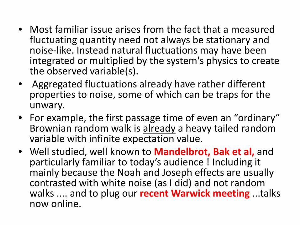
• Most familiar issue arises from the fact that a measured
fluctuating quantity need not always be stationary and noise-like. Instead natural fluctuations may have been integrated or multiplied by the system's physics to create the observed variable(s).
• Aggregated fluctuations already have rather different properties to noise, some of which can be traps for the unwary.
• For example, the first passage time of even an “ordinary” Brownian random walk is already a heavy tailed random variable with infinite expectation value.
• Well studied, well known to Mandelbrot, Bak et al, and particularly familiar to today’s audience ! Including it mainly because the Noah and Joseph effects are usually contrasted with white noise (as I did) and not random walks .... and to plug our recent Warwick meeting ...talks now online.
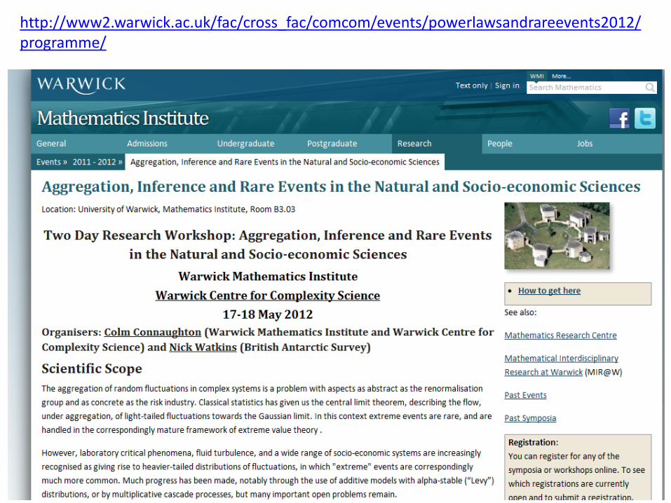
http://www2.warwick.ac.uk/fac/cross_fac/comcom/events/powerlawsandrareevents2012/programme/
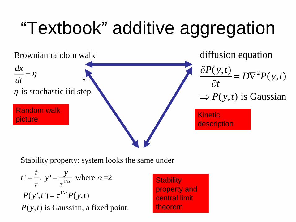
“Textbook” additive aggregation Brownian random walk
is stochastic iid step
dxdt
η
η
= 2
diffusion equation( , ) ( , )
( , ) is Gaussian
P y t D P y tt
P y t
∂= ∇
∂⇒
1/
1/
Stability property: system looks the same under
' , ' where =2
( ', ') ( , )( , ) is Gaussian, a fixed point.
t yt y
P y t P y tP y t
α
α
ατ τ
τ
= =
=
Random walk picture Kinetic
description
Stability property and central limit theorem
MEMORY IS NOT (ALWAYS) FRACTALITY
• A more subtle problem arises from the fact that a few
of the very popular diagnostics are constructed to measure self-similarity , while most (e.g. R/S, DFA) in fact measure long-range dependence, so some confusion can arise when interpreting their outputs in systems where these two properties are not synonymous.
• Discussed in Franzke et al, Phil Trans A, 2012; see also Mercik et al, ”Enigma of self-similarity of fractional Levy stable motions”, Acta Phys. Pol. B 34 3773 (2003).
FRACTAL NOISE MODELS: HOW TO CHOOSE ?
• Several models modify the Brownian random walk,
including those for “anomalous diffusion”. In Watkins et al, PRE, 2009 we attempted to present a classification, which needs some correction.
• Three particularly important classes of such models are: additive and undamped, including fractional stable models,
the fractional CTRW, and generalised shot noises additive and mean reverting (damped) models like the
Ornstein-Uhlenbeck process multiplicative processes.
• Important to dispel the misconception that
such models are ``just statistics", as many embody a close correspondence with a physical scenario, which can be used as a guide when trying to choose the most suitable one to use, and which will bite back if you ignore it !
ADDITIVE UNDAMPED MODELS
• The variance of an additive stochastic process
with no damping will tend to grow with time. • It is thus a model of diffusion. Not so obvious
that it will be a time series model. • Recap links between Langevin and Fokker-
Planck descriptions of diffusion, and the central limit theorem and scaling.

Brownian Case Brownian random walk
is stochastic iid step
dxdt
η
η
= 2
diffusion equation( , ) ( , )
( , ) is Gaussian
P y t D P y tt
P y t
∂= ∇
∂⇒
1/
1/
Stability property: system looks the same under
' , ' where =2
( ', ') ( , )( , ) is Gaussian, a fixed point.
t yt y
P y t P y tP y t
α
α
ατ τ
τ
= =
=
Random walk Kinetic description
Stability property and central limit theorem
• In Brownian case the three legs are (by now)
very well studied and relate to each other. • When we go beyond Brownian motion, it is
not self-evident that can maintain all 3 properties ... and in fact when we look at the models that have been developed we will see that they don’t.
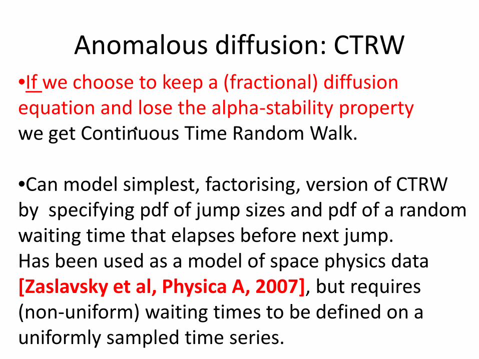
Anomalous diffusion: CTRW •If we choose to keep a (fractional) diffusion equation and lose the alpha-stability property we get Continuous Time Random Walk. •Can model simplest, factorising, version of CTRW by specifying pdf of jump sizes and pdf of a random waiting time that elapses before next jump. Has been used as a model of space physics data [Zaslavsky et al, Physica A, 2007], but requires (non-uniform) waiting times to be defined on a uniformly sampled time series.
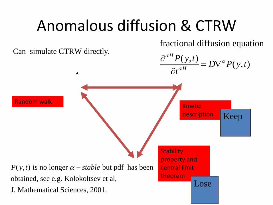
Anomalous diffusion & CTRW Can simulate CTRW directly.
fractional diffusion equation( , ) ( , )
H
H
P y t D P y tt
αα
α
∂= ∇
∂
( , ) is no longer but pdf has been obtained, see e.g. Kolokoltsev et al,J. Mathematical Sciences, 2001.
P stabley t α −
Random walk Kinetic description
Stability property and central limit theorem
Keep
Lose
2α =α H
1/ 2H =1/H dα= +
2t pp∇ = ∂
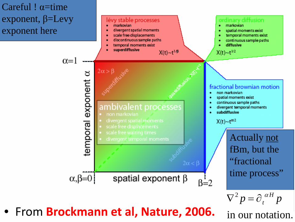
• From Brockmann et al, Nature, 2006.
'/H d α=
0 2α< ≤ 1/H α=
t ppα∇ = ∂
2α =
0 2α< ≤
0 1H≤ ≤
0 1H≤ ≤
Ordinary Levy Motion
Bachelier -Wiener Brownian Motion
2 Htp pα∇ ∂=
Careful ! α=time exponent, β=Levy exponent here
Actually not fBm, but the “fractional time process”
2
in our notation.
Ht pp α∇ ∂=
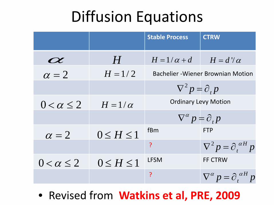
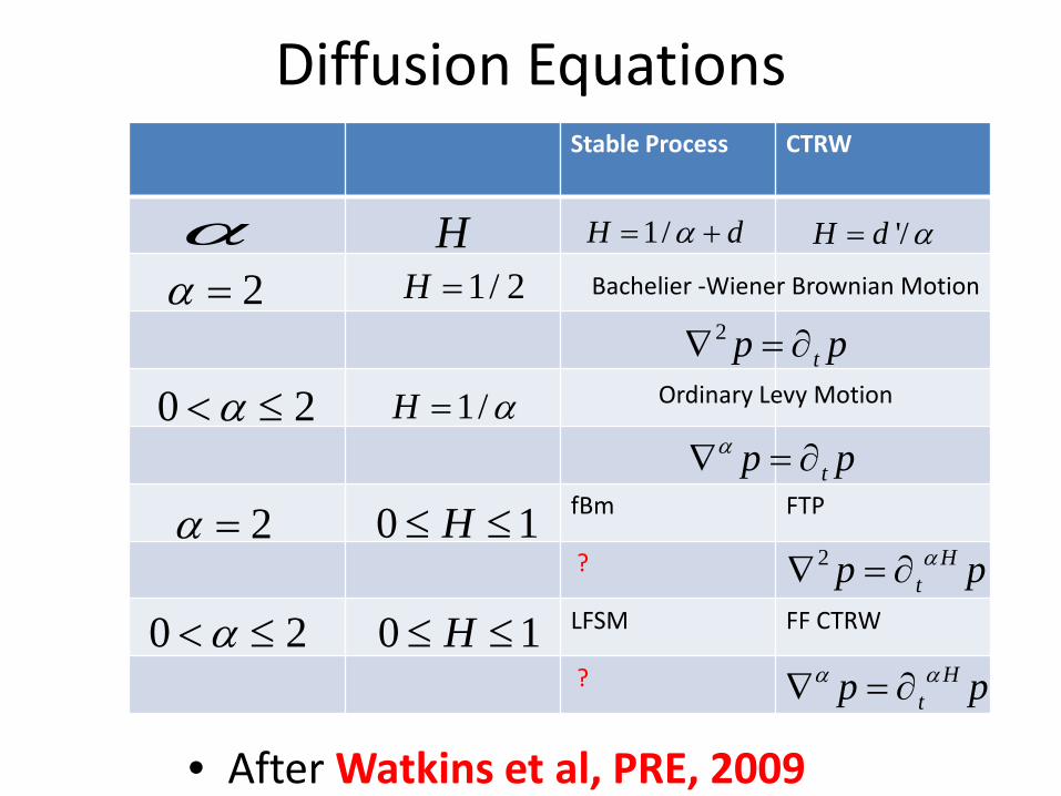
Diffusion Equations Stable Process
CTRW
fBm FTP
?
LFSM FF CTRW
?
2α =α H
1/ 2H =1/H dα= +
2t pp∇ = ∂
• Revised from Watkins et al, PRE, 2009
'/H d α=
0 2α< ≤ 1/H α=
t ppα∇ = ∂
2α =
0 2α< ≤
0 1H≤ ≤
0 1H≤ ≤
Ordinary Levy Motion
Bachelier -Wiener Brownian Motion
2 Htp pα∇ ∂=
Htp pα α∇ ∂=

Stable processes: linear fractional stable motion
•Conversely if we lose the diffusion equation but keep the alpha-stability property we get the family of fractional stable motions. Has been proposed as a model of AE, e.g. Watkins et al, Space Science Reviews, 2005. Biggest deficiency is shape of the pdfs, which are heavier-tailed than reality (see e.g. Rypdal & Rypdal, 2011). Fix-up of truncated Levy approach less satisfactory than some others here.
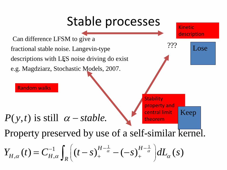
Stable processes Can difference LFSM to give a fractional stable noise. Langevin-typedescriptions with LFS noise driving do existe.g. Magdziarz, Stochastic Models, 2007.
???
1 11
( , ) is still by use of a self-similar kernel.
( ) ( ) (
.Property preserve
) (
d
)H HH H R
P y t
Y t
st
C t s s dL
able
sα αα α α
α
− −− , , + + − −
−
= −∫
Random walks
Kinetic description
Stability property and central limit theorem
Lose
Keep

Kinetic picture ? Early work on fBm for example proposed that a diffusion equation with a diffusion coefficient with power law time dependence would describe it, see also Watkins et al, 2009. WRONG !, as this describes the pdf but not the correct temporal structure e.g. first passage time etc. See e.g. Lim and Muniandy, PRE, 2002.
1( ) Ht P H t D Pα αα −∂ = ∂
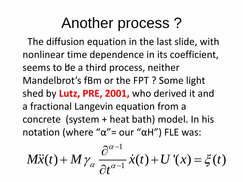
Another process ? The diffusion equation in the last slide, with nonlinear time dependence in its coefficient, seems to be a third process, neither Mandelbrot’s fBm or the FPT ? Some light shed by Lutz, PRE, 2001, who derived it and a fractional Langevin equation from a concrete (system + heat bath) model. In his notation (where “α”= our “αH”) FLE was: 1
1( ) ( ) '( ) ( )x t M x t U x tt
Mα
α αγ ξ−
−
∂+ + =
∂
Diffusion Equations Stable Process
CTRW
fBm FTP
?
LFSM FF CTRW
?
2α =α H
1/ 2H =1/H dα= +
2t pp∇ = ∂
• After Watkins et al, PRE, 2009
'/H d α=
0 2α< ≤ 1/H α=
t ppα∇ = ∂
2α =
0 2α< ≤
0 1H≤ ≤
0 1H≤ ≤
Ordinary Levy Motion
Bachelier -Wiener Brownian Motion
2 Htp pα∇ ∂=
Htp pα α∇ ∂=
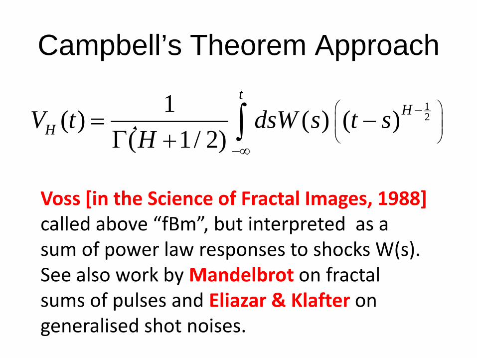
Campbell’s Theorem Approach
Voss [in the Science of Fractal Images, 1988] called above “fBm”, but interpreted as a sum of power law responses to shocks W(s). See also work by Mandelbrot on fractal sums of pulses and Eliazar & Klafter on generalised shot noises.
12
1( ) ( ) ( )( 1/ 2)
tH
HV t dsW s t sH
−
−∞
= −Γ + ∫
ADDITIVE DAMPED MODELS
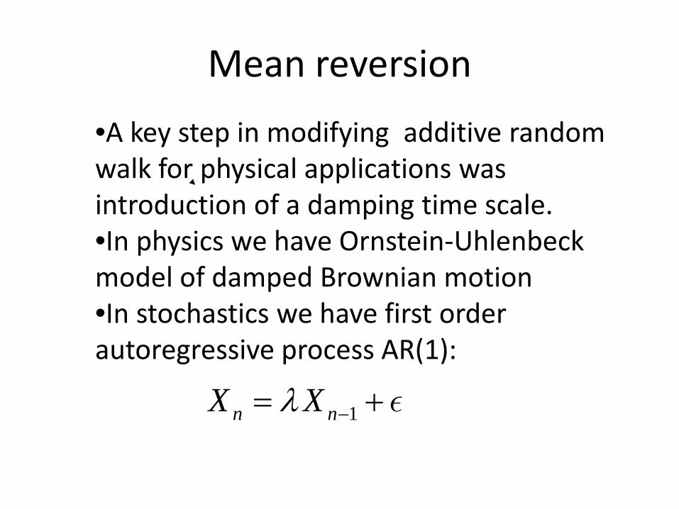
Mean reversion •A key step in modifying additive random walk for physical applications was introduction of a damping time scale. •In physics we have Ornstein-Uhlenbeck model of damped Brownian motion •In stochastics we have first order autoregressive process AR(1):
1n nX Xλ −= +
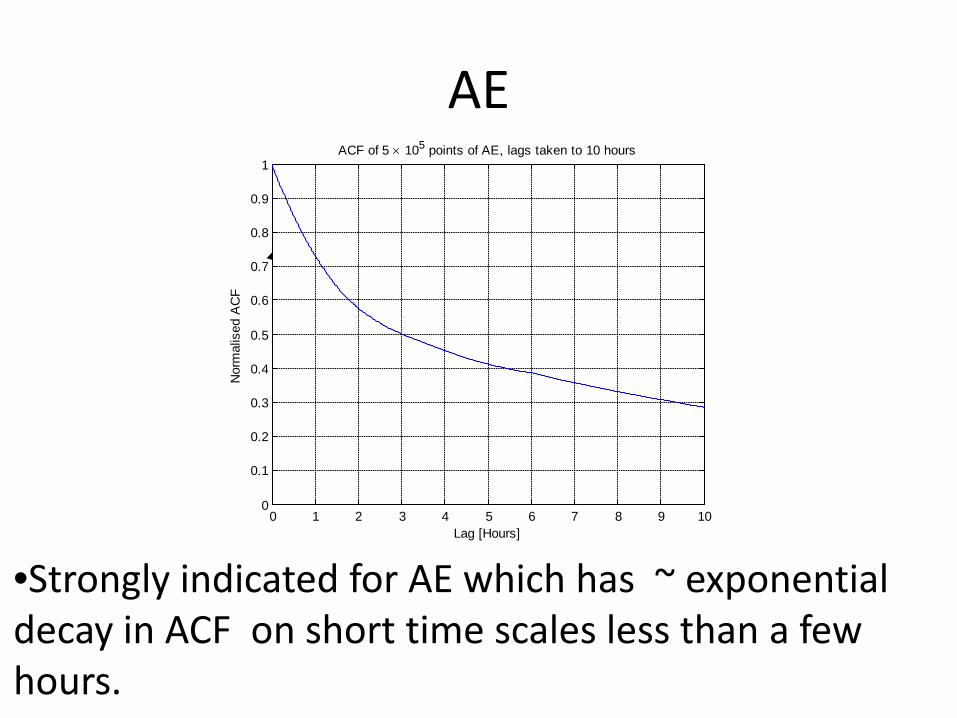
AE
•Strongly indicated for AE which has ~ exponential decay in ACF on short time scales less than a few hours.
0 1 2 3 4 5 6 7 8 9 100
0.1
0.2
0.3
0.4
0.5
0.6
0.7
0.8
0.9
1
Nor
mal
ised
AC
F
Lag [Hours]
ACF of 5 × 10⁵ points of AE, lags taken to 10 hours

MULTIPLICATIVE MODELS
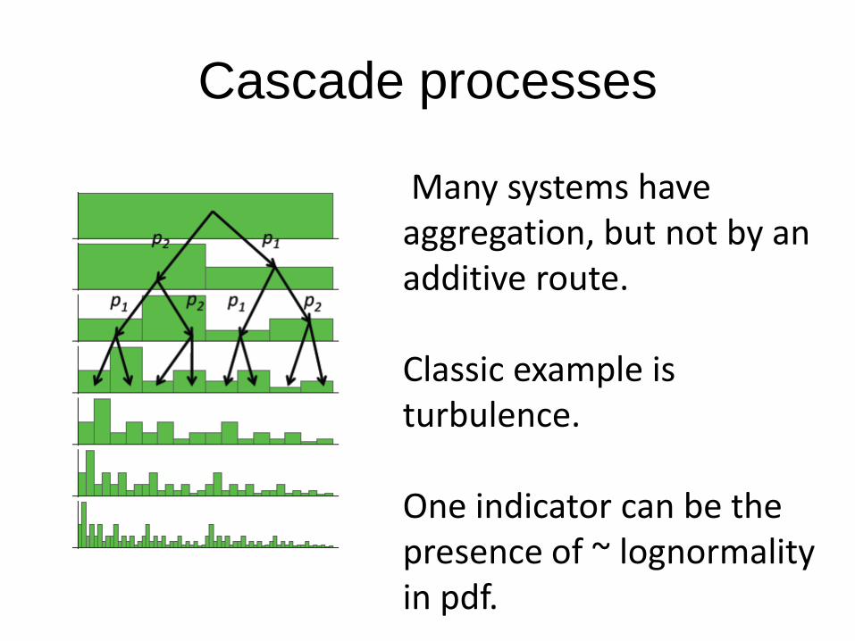
Cascade processes
Many systems have aggregation, but not by an additive route. Classic example is turbulence. One indicator can be the presence of ~ lognormality in pdf.
Modelling AE
An interesting recent synthesis of these approaches has been combination of mean reversion and a multifractal noise by Rypdal and Rypdal, 2011 to model AE. As in finance a log transformation was first employed to give a series with near-stationary increments.
Summary
Why stochastic models ? Textbook stochastic models Noah, Joseph and volatility bunching A physics of fractals ? From fractals back to physics ? Pitfalls: 1. Walks are not noises 2. Memory not always self-similarity 3. Choice of fractal models

http://www2.warwick.ac.uk/fac/cross_fac/comcom/events/powerlawsandrareevents2012/programme/