On complex behavior and exchange rate dynamics

On complex behavior and exchange rate dynamics

Brian Schwartz, Shahriar Yousefi *

The Econometric Group, Department of Economics, University of Southern Denmark, Campusvej 55, Odense M 5230, Denmark

Abstract

The presence of nonlinear dependence and lower dimensional complex dynamics in exchange rate dynamics is

studied. A series of empirical and theoretical difficulties are elaborated on.

� 2003 Elsevier Science Ltd. All rights reserved.

1. Introduction

Financial econometrics is known to be a fairly empirical discipline with occasional elements of ad hoc reasoning (see

for instance the introduction to Campbell et al. [1]). From a theoretical point of view, the proposition that financial

markets are efficient, constitute the cornerstone of mainstream reasoning in this field. Nevertheless, when the matter is

viewed from a fairly broader perspective, it appears that there are various technical considerations, evidence of

dominating empirical regularities and theoretical models in the literature that seriously erode the trust in this hy-

pothesis. In such cases, basic arguments against this theory are usually associated with the persistent neglect of the

influence of any systematic element in the dynamics of prices (or their increments) and their apparent deviation from

the fundamental values. The interested reader is recommended to consult Refs. [1–8] for elaborations and further

details.

While recognizing the central position of this theory in the literature, it is only fair to state that although this theory

remains to be one of the unqualified successes of the mainstream economics, the idea of efficient markets is regularly a

matter of controversy and subject for discussion among scholars. Apparently, the main debate that arises from these

exchanges of ideas is focused on coherent methodological approaches and eventually the existence of persistent em-

pirical evidence in support of these approaches.

Regarding the empirical evidence, it is worth noting that there are various nontrivial difficulties to be confronted in

the analysis of the actual dynamics of speculative financial assets [1,9,10]. For instance it is widely known that problems

related to the quality (and lack of sufficient amount) of data, the issue of appropriate level of disaggregation, the proper

definition of (and methods for) detecting white noise, the irregular and unexpected perturbations in definitions of

variables, the issue of temporal and spatial heterogeneity of variables (and agents) along a series of other issues create

considerable obstacles for constructing a meaningful and coherent statistical theory about the dynamics of speculative

financial assets. Perhaps the most significant features of the time series associated with the prices of these assets is their

tendency to exhibit higher level of volatility (which is a measure of market fluctuations averaged over a given time

interval), while the empirical distribution of their increments (or their simple transformations) tends to be highly

leptokurtosis (in other words they are possessing higher peaks around the mean and fatter tails than the normal dis-

tribution). Furthermore, evidence on the presence of nonlinear serial dependence in financial data has been reported in

the literature since early 1980s [11] while theoretical studies devoted to this issue have been circulated in the time series

* Corresponding author. Tel.: +45-65-503342; fax: +45-66-158790.

E-mail address: [email protected] (S. Yousefi).

0960-0779/03/$ - see front matter � 2003 Elsevier Science Ltd. All rights reserved.

doi:10.1016/S0960-0779(02)00673-2

Chaos, Solitons and Fractals 18 (2003) 503–523

www.elsevier.com/locate/chaos

mail to: [email protected]

literature since the early contribution of Brillinger [12]. This study eventually motivated the works of Rao and Gabr [13]

and Hinich [14] on devising specific tests for detecting the presence of nonlinear dependence.

It is fair to assume that most experienced econometricians are familiar with the fact that many of these features are

also associated with the empirical studies of the dynamics of foreign exchange markets [15–20]. With regard to the

recent developments in this field, there have certainly been some discussions among economists concerning the ap-

plication of the theory of nonlinear dynamics (and the associated theories of chaos and complexity) in dealing with

these issues [5,21–25]. These discussions, alongside the facts such as: the ever increasing number of floating currencies

since 1970s, the emergence of significant and persistent trade imbalances among major economies in 1980s and the

growing interdependencies among world economies as a consequence of rapid globalization in 1990s, have transformed

the study of the dynamics of foreign exchange markets into a promising field with particular potential for developing

(and applying) alternative econometric techniques based on the insight provided by the recent advances in the larger

field of nonlinear dynamics.

Over the past 10 years or so, a series of studies have been published with particular focus on the issue of detecting

chaotic dynamics in exchange rates [22,24–32]. In retrospect, the main contribution of these studies was to introduce

(and give some empirical content to) a few new techniques (that were originally developed in the field of nonlinear

dynamics) into the finance and econometric literature. The most frequently applied techniques in this body of literature

range from phase space reconstruction procedure based on the application of Taken�s embedding theorem, to separate

estimation of largest Lyapunov exponents, using data dependent models for estimating the dimension of underlying

economic system and finally devising methods for the detection of nonlinear serial dependence.

The empirical findings of these contributions are mixed and (occasionally) associated with a certain na€ııve enthusiasm

in interpreting the results obtained from samples with inadequate sizes and quality. Although the initial reactions to

these findings have been mixed, the preponderance of the opinions has been biased towards skeptical rejection of their

significance. The criticism is predominantly associated with issues such as illicit application of the techniques, occa-

sional neglect of regular econometric insight (nonstationarity, presence of noise, etc.), apparent shortcomings in pro-

viding a germane framework for statistical inference (due to the lack of a coherent distributional theory), poor

forecasting performances and relying on limited number of parameter combinations in estimation procedures.

As far as the present work is concerned, the main intention is to elaborate on various features and statistical time

series characteristics of exchange rates by directing the focus towards the search for a data dependent measurable

indication of chaos in their dynamics. As mentioned before, different scholars have addressed this issue in recent years.

Nevertheless we attempt here to give some new perspectives on how an extension of this sort of studies should be

associated with a clearly defined working hypothesis, a coherent procedure for the empirical investigation, a proper

discussion of possible limitations of the applied techniques and finally an effort to fit the entire analysis into a larger

picture associated with the previous contributions to the literature.

In order to proceed, an operational definition of chaos is adopted in accordance to what seems to be commonly

accepted in the literature on nonlinear dynamics and econometrics [32]. In this context, a chaotic signal is defined as a

seemingly random and irregular signal generated by a nonlinear deterministic process with certain properties such as

association with an irregular attractor with a (low) fractal dimension and the ability to exhibit sensitive dependence on

initial conditions. Consequently, it is fair to assume that a time series with a seemingly random and irregular pattern, an

inherent nonlinear dependence, lower estimates for correlation dimension, and positive estimates of largest Lyapunov

exponent, is prone to be the manifestation of an underlying chaotic dynamics.

In the following parts, efforts are confined to an investigation of the presence of these features among certain ex-

change rate series. Although the treatment is in no way self-contained, much effort is invested to: lay out a concise

description of the applied methods in the analysis, present a balanced account of the underlying reasoning behind these

methods, outline their limitations, specify their significance and finally provide references to more detailed sources for

further consultations. The theoretical foundation of this study (Section 2) provides a brief outline of the basic tech-

niques, analytical results and statistical tools that are applied in the analysis. Section 3 begins by introducing the data

and continues by applying the techniques mentioned in Section 2 to foreign exchange rates. Section 4 puts the results in

perspective and concludes by initiating a discussion on their significance.

2. Methodology

This part describes the underlying theoretical assumptions, numerical techniques and statistical tools that are ap-

plied in the analysis. These are the phase space reconstruction technique, numerical procedures for estimating corre-

lation dimension, BDS test for nonlinear dependence, and numerical procedures for estimating largest Lyapunov

exponent.

504 B. Schwartz, S. Yousefi / Chaos, Solitons and Fractals 18 (2003) 503–523

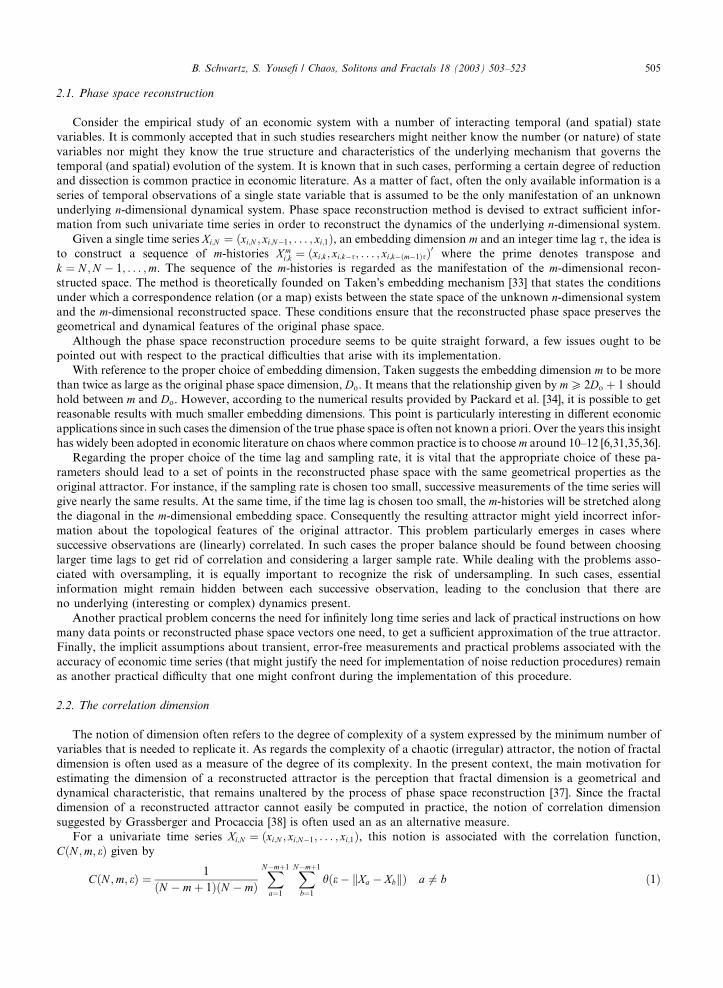
2.1. Phase space reconstruction

Consider the empirical study of an economic system with a number of interacting temporal (and spatial) state

variables. It is commonly accepted that in such studies researchers might neither know the number (or nature) of state

variables nor might they know the true structure and characteristics of the underlying mechanism that governs the

temporal (and spatial) evolution of the system. It is known that in such cases, performing a certain degree of reduction

and dissection is common practice in economic literature. As a matter of fact, often the only available information is a

series of temporal observations of a single state variable that is assumed to be the only manifestation of an unknown

underlying n-dimensional dynamical system. Phase space reconstruction method is devised to extract sufficient infor-

mation from such univariate time series in order to reconstruct the dynamics of the underlying n-dimensional system.

Given a single time series Xi;N ¼ ðxi;N ; xi;N�1; . . . ; xi;1Þ, an embedding dimension m and an integer time lag s, the idea is

to construct a sequence of m-histories Xmi;k ¼ ðxi;k ; xi;k�s; . . . ; xi;k�ðm�1ÞsÞ0 where the prime denotes transpose and

k ¼ N ;N � 1; . . . ;m. The sequence of the m-histories is regarded as the manifestation of the m-dimensional recon-

structed space. The method is theoretically founded on Taken�s embedding mechanism [33] that states the conditions

under which a correspondence relation (or a map) exists between the state space of the unknown n-dimensional system

and the m-dimensional reconstructed space. These conditions ensure that the reconstructed phase space preserves the

geometrical and dynamical features of the original phase space.

Although the phase space reconstruction procedure seems to be quite straight forward, a few issues ought to be

pointed out with respect to the practical difficulties that arise with its implementation.

With reference to the proper choice of embedding dimension, Taken suggests the embedding dimension m to be more

than twice as large as the original phase space dimension, Do. It means that the relationship given by mP 2Do þ 1 should

hold between m and Do. However, according to the numerical results provided by Packard et al. [34], it is possible to get

reasonable results with much smaller embedding dimensions. This point is particularly interesting in different economic

applications since in such cases the dimension of the true phase space is often not known a priori. Over the years this insight

has widely been adopted in economic literature on chaos where common practice is to choose m around 10–12 [6,31,35,36].

Regarding the proper choice of the time lag and sampling rate, it is vital that the appropriate choice of these pa-

rameters should lead to a set of points in the reconstructed phase space with the same geometrical properties as the

original attractor. For instance, if the sampling rate is chosen too small, successive measurements of the time series will

give nearly the same results. At the same time, if the time lag is chosen too small, the m-histories will be stretched along

the diagonal in the m-dimensional embedding space. Consequently the resulting attractor might yield incorrect infor-

mation about the topological features of the original attractor. This problem particularly emerges in cases where

successive observations are (linearly) correlated. In such cases the proper balance should be found between choosing

larger time lags to get rid of correlation and considering a larger sample rate. While dealing with the problems asso-

ciated with oversampling, it is equally important to recognize the risk of undersampling. In such cases, essential

information might remain hidden between each successive observation, leading to the conclusion that there are

no underlying (interesting or complex) dynamics present.

Another practical problem concerns the need for infinitely long time series and lack of practical instructions on how

many data points or reconstructed phase space vectors one need, to get a sufficient approximation of the true attractor.

Finally, the implicit assumptions about transient, error-free measurements and practical problems associated with the

accuracy of economic time series (that might justify the need for implementation of noise reduction procedures) remain

as another practical difficulty that one might confront during the implementation of this procedure.

2.2. The correlation dimension

The notion of dimension often refers to the degree of complexity of a system expressed by the minimum number of

variables that is needed to replicate it. As regards the complexity of a chaotic (irregular) attractor, the notion of fractal

dimension is often used as a measure of the degree of its complexity. In the present context, the main motivation for

estimating the dimension of a reconstructed attractor is the perception that fractal dimension is a geometrical and

dynamical characteristic, that remains unaltered by the process of phase space reconstruction [37]. Since the fractal

dimension of a reconstructed attractor cannot easily be computed in practice, the notion of correlation dimension

suggested by Grassberger and Procaccia [38] is often used an as an alternative measure.

For a univariate time series Xi;N ¼ ðxi;N ; xi;N�1; . . . ; xi;1Þ, this notion is associated with the correlation function,

CðN ;m; eÞ given by

CðN ;m; eÞ ¼ 1

ðN � mþ 1ÞðN � mÞXN�mþ1

a¼1

XN�mþ1

b¼1

hðe � kXa � XbkÞ a 6¼ b ð1Þ

B. Schwartz, S. Yousefi / Chaos, Solitons and Fractals 18 (2003) 503–523 505

where m is an embedding dimension, Xa and Xb are vectors among m-histories from the embedding matrix, e is the radius

of an infinitesimal m-dimensional hypersphere, k k is the norm operator and h is an indicator that is set to 1 for positive

arguments and zero otherwise. Furthermore, it has been shown that CðN ;m; eÞ ¼ geDc , where g is a constant and Dc is

the correlation dimension.

Referring to the choice of norm, the norm theorem given in Brock [39], states the condition under which the cor-

relation function remains independent of the choice of norm. However, these conditions are hardly met in short noisy

time series, a category, in which financial data are often being put in. As a matter of fact, simulations in Kugiumtzis [40]

show that this theorem is not valid for short noisy time series. According to this study, most reliable results are obtained

by using the Euclidian norm under such circumstances. Based on this insight, in the present work, the Euclidian norm is

adopted in the calculation of the correlation dimension.

Obviously, the correlation function measures the probability of any two m-histories being closer than e to each other.

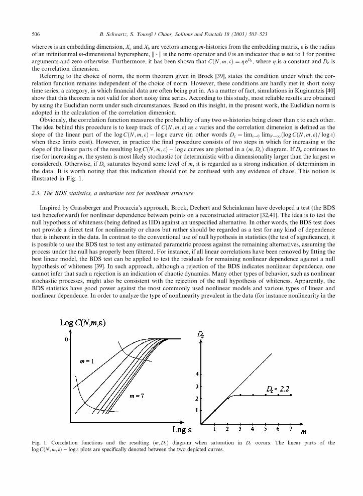
The idea behind this procedure is to keep track of CðN ;m; eÞ as e varies and the correlation dimension is defined as the

slope of the linear part of the logCðN ;m; eÞ � log e curve (in other words Dc ¼ lime!0 limN!1ðlogCðN ;m; eÞ= log eÞwhen these limits exist). However, in practice the final procedure consists of two steps in which for increasing m the

slope of the linear parts of the resulting logCðN ;m; eÞ � log e curves are plotted in a ðm;DcÞ diagram. If Dc continues to

rise for increasing m, the system is most likely stochastic (or deterministic with a dimensionality larger than the largest mconsidered). Otherwise, if Dc saturates beyond some level of m, it is regarded as a strong indication of determinism in

the data. It is worth noting that this indication should not be confused with any evidence of chaos. This notion is

illustrated in Fig. 1.

2.3. The BDS statistics, a univariate test for nonlinear structure

Inspired by Grassberger and Procaccia�s approach, Brock, Dechert and Scheinkman have developed a test (the BDS

test henceforward) for nonlinear dependence between points on a reconstructed attractor [32,41]. The idea is to test the

null hypothesis of whiteness (being defined as IID) against an unspecified alternative. In other words, the BDS test does

not provide a direct test for nonlinearity or chaos but rather should be regarded as a test for any kind of dependence

that is inherent in the data. In contrast to the conventional use of null hypothesis in statistics (the test of significance), it

is possible to use the BDS test to test any estimated parametric process against the remaining alternatives, assuming the

process under the null has properly been filtered. For instance, if all linear correlations have been removed by fitting the

best linear model, the BDS test can be applied to test the residuals for remaining nonlinear dependence against a null

hypothesis of whiteness [39]. In such approach, although a rejection of the BDS indicates nonlinear dependence, one

cannot infer that such a rejection is an indication of chaotic dynamics. Many other types of behavior, such as nonlinear

stochastic processes, might also be consistent with the rejection of the null hypothesis of whiteness. Apparently, the

BDS statistics have good power against the most commonly used nonlinear models and various types of linear and

nonlinear dependence. In order to analyze the type of nonlinearity prevalent in the data (for instance nonlinearity in the

Fig. 1. Correlation functions and the resulting ðm;DcÞ diagram when saturation in Dc occurs. The linear parts of the

logCðN ;m; eÞ � log e plots are specifically denoted between the two depicted curves.


mean or in the variance), one would need to model different nonlinear processes directly. Since this issue is beyond the

scope of this work, our efforts will be confined to testing for general nonlinearity. The interested reader is recommended

to consult other sources such as Refs. [1,24] for further elaboration on this issue.

The BDS test is based on the notion of correlation function and Brock et al. [41] shows that under the null hy-

pothesis of whiteness,

W ðN ;m; eÞ ¼ffiffiffiffiffiffiffiffiffiffiffiffiffiffiffiffiffiffiffiffiffiffiN � mþ 1

p CðN ;m; eÞ � CðN ; 1; eÞm

r̂rðN ;m; eÞ ð2Þ

follows a limiting standard normal distribution with mean zero and unit variance. In other words

limN!1 W ðN ;m; eÞ Nð0; 1Þ; 8m; e, indicating that the BDS statistic follows the standard normal distribution as-

ymptotically. r̂rðN ;m; eÞ is an estimate of the asymptotic standard deviation of CðN ;m; eÞ � CðN ;m; eÞm and is consis-

tently estimated by

r̂r2ðN ;m; eÞ ¼ 4 km"

þ 2Xm�1

r¼1

km�rc2j þ ðm� 1Þ2c2m � m2kc2m�2

#ð3Þ

where C ¼ E½CðN ;m; eÞ� can be consistently estimated by CðN ;m; eÞ for m ¼ 1 while k ¼RðF ðzþ eÞ � F ðz� eÞÞ2

can be

estimated by

kðN ; eÞ ¼ 6

N � mþ 1ðN � mÞðN � m� 1ÞXN�m�1

a¼1

XN�m

b¼aþ1

XN�m�1

c¼bþ1

½hðe � kXa � XbkÞhðe � kXb � XckÞ

þ hðe � kXa � XckÞhðe � kXc � XbkÞ þ hðe � kXb � XakÞhðe � kXa � XckÞ�:

Although the BDS test seems to be powerful against different types of linear and nonlinear dependency [1], Brock

[39] states that the specification of possible nonlinear dependency among the observations depends on the removing all

linear correlations that may cause the null hypothesis to be rejected. He also argue that possible nonlinear structures

should be unaffected by implementing a linear filtering process. Consequently, it is fair to infer that the asymptotic

distribution of the BDS statistic applies to the residuals of linear regressions in the same way as the original data.

Removing all linear structure is difficult, but a good approximation can be achieved by using an autoregressive moving

average (ARMA) fit on stationary data. The BDS test can then be run over the residuals of the regression with the

alternative hypothesis of general nonlinear dependence among data. With the assumption that the residuals are filtered

for linear dependence, it is reasonable to assert that any resulting dependence found in the residuals must be nonlinear.

In several cases, researchers have addressed the issue of the existence of time-varying variance in the time series and

in a few cases, the matter is handled by performing the BDS test on ARCH or GARCH (see Bollerslev [42] for details

about these models) filtered data in order to test for remaining nonlinear dependence [24,25,30,32]. The literature is not

conclusive on the usefulness of this approach. For instance, as indicated by Brock et al. [32], ARCH and GARCH

residuals seem to bias the BDS statistic for unknown reasons. In the present work, an alternative approach originally

proposed by Hsieh has been applied in order to deal with time-varying variance [24,25]. The idea is to use a very simple

model of exogenous heteroscedasticity where time is assumed to affect the variance of exchange rate returns in such a

way that, within a month the variance structure remains stable. In short, before performing the BDS test, the (linear)

filtered log-returns should be standardized by dividing each observation by the monthly standard deviation. Conse-

quently, in the present work the BDS test will be performed both on (linear) filtered log-returns and variance-stan-

dardized (linear) filtered log-returns. If the null hypothesis is rejected in the first case, the alternative hypothesis states

that data exhibits general nonlinear dependence. If, at the same time, the null hypothesis is not rejected in the second

case, it is fair to conclude that dependency in the exchange rate log-returns is caused by a changing variance. On the

other hand, if the null hypothesis is also rejected in the second case, it is reasonable to assert that the standardization

procedure has not been adequate in removing all nonlinear dependence. In other words, the remaining nonlinear de-

pendency in the data may, or may not, origin from an underlying chaotic dynamics. Thus, a BDS rejection is not direct

evidence of nonlinear dependence in the mean. In short, although nonlinearity in the mean is consistent with a BDS

rejection, a BDS rejection is not necessarily consistent with nonlinearity in the mean.

2.4. Estimating largest Lyapunov exponent

A dominant approach in the literature relies on the notion of sensitivity to initial conditions and the perception that

chaos will exist if nearby trajectories diverge (exponentially). As a matter of fact, the presence of the sensitivity to initial

conditions signifies local instability of the system that is manifested in rapid (local) divergence of trajectories. One of the


serious consequences of the existence of sensitivity to initial conditions is the systematic loss of predictability of the

system over time. The notion of Lyapunov spectrum is often used to quantify and detect this phenomenon. Lyapunov

exponents are derived from k ¼ limn!1 lnðkDf nðxÞ~vvkÞ=n where D signifies the derivative, k k is the Euclidian norm, f n

is the nth iteration of dynamical system f with initial conditions in point x and~vv is a direction vector. If the largest real

part of these exponents is positive then the system exhibits sensitivity to initial conditions. In this case, the speed by

which the systematic loss of predictability is materialized, depends on the magnitude of the largest real part of these

exponents. In short, larger magnitudes imply faster decay in predictability.

Obviously, this mechanism requires knowledge of the analytical structure of the underlying dynamics. In cases when

the true dynamics are not known, a practical remedy is to devise methods for extracting information about the rates of

divergence between nearby orbits from a sequence of observed data. Over the years, an algorithm suggested by Wolf

et al. [43] has been used for this purpose. Apparently, the application of this routine is associated with a few practical

difficulties [44–46].

In order to remedy these difficulties, in this work the search for indications of sensitivity to initial conditions is based

on an algorithm that is a slightly modified version of two similar algorithms suggested by Rosenstein et al. [44] and

Kantz [45]. The basic idea is to trace the distance in between a reference point X0 and its neighbor, Xj, after n time steps.

Set djðX0;Xj; nÞ to be this distance in the reconstructed phase space and let eðX0;XjÞ denote the initial distance between

X0 and Xj. In this case, djðX0;Xj; nÞ should grow exponentially by the largest Lyapunov exponent kmaxðX0Þ, or as it might

be expressed in logarithm scale

ln djðX0;Xj; nÞ � kmaxðX0Þnþ ln eðX0;XjÞ ð4Þ

Consequently, it is postulated that if this linear pattern is persistent for a number of time steps n, the estimated slope

is an estimate for the largest Lyapunov exponent.

Rosenstein et al. [44] and Kantz [45] procedures differs with respect to the number of neighbors that are considered.

While the first procedure trace the nearest neighbor, the second one keeps track of all neighbors within a neighborhood

ball BðX0Þ. By taking an average of all neighbors within the neighborhood, this method seems more robust against noisy

elements.

The procedure can be formalized in devising a line S, as a function of the number of time steps, number of ob-

servations, the embedding dimension and radius of the ball B (which is an indicator for the size of the neighborhood):

SðDn;N ;m; eÞ ¼ 1

N � mþ 1

XN�mþ1

i0¼1

ln1

jBðXi0ÞjX

Xj2BðXi0 Þkxði0þDn;1Þ

0@ � xðjþDn;1Þk

1A ð5Þ

jBðÞj is the total number of neighbors in the neighborhood B (a ball with diameter e) of the reference vector Xi0 . xði0 ;1Þis the most recent, element in the reference vector, Xi0 and xði0þDn;1Þ is the first observation outside the time span covered

by the reference vector. Thus, for a series of daily observations, xði0 ;1Þ is the observation at time t and xði0þDn;1Þ is the

observation at time t þ 1. In the same way, xðj;1Þ is the first and most recent element of the neighboring vector, Xj, and

xðjþDn;1Þ is the first observation outside the time span covered by Xj.

As an extension of this procedure, Kantz and Schreiber [47] propose to discard all points that do not have at least

nfmin neighbors. Introducing a neighborhood might cause problems with regard to the unjustified (and perhaps fre-

quent) exclusion of points that are located in the less populated areas of the reconstructed phase space. Obviously, in

these cases increasing the radius of the ball BðX0Þ is an option. But this might again cause another problem in densely

populated areas of the phase space where a relatively sharp increase in the number of neighbors to each point can blur

any possible dynamic element when averaging.

On the other hand, Rosenstein et al. [44] estimate of kmax might suffer from an inherent source for bias. Since the

algorithm searches for the nearest neighbor (regardless of its actual location), a point located in sparsely populated area

of the phase space risk to be associated with a quite distanced neighbor. When these two trajectories are traced in time

and the resulting distance is measured, there may be no sign of exponential divergence, even if the time series is known

to be chaotic. This might be a serious cause for bias in the estimation of kmax.

Despite the minor disadvantages of the Kantz [45] procedure, a slightly modified version of this procedure will be

used as the basic instrument in the estimation of kmax in present work. It is worth noting that, Kantz and Schreiber [47]

recommend truncating the algorithm as soon as a limited number of reference points with at least nfmin neighbors, are

reached. This measure is introduced to handle the computational intensiveness of the original procedure. However, this

step might ignore vital information associated with certain parts of the reconstructed attractor. As a result, no limit, set

on the number of reference points, is included in our estimation of kmax. Another problem emerges with regard to the

proper choice of minimum embedding dimension as well as the optimal radius. Kantz and Schreiber [47] recommend


computing SðDnÞ for a variety of both values. However, in order to reduce the total computation time, in present work

the radius e is kept unchanged and only m varies.

In order to illustrate the reliability of the modified algorithm in estimating kmax, the modified algorithm is applied on

two artificial chaotic time series generated by the logistic map

xtþ1 ¼ lxtð1 � xtÞ for l ¼ 4

and Hennon map

xtþ1 ¼ 1 � ax2t þ yt

ytþ1 ¼ bxt

for a ¼ 1:4 and b ¼ 0:3

Two time series are constructed by iterating both maps 2.000 times and the first 1.000 points are excluded. Em-

bedding dimensions of m ¼ 2–5 are considered and e is chosen so that 80–100% of all reference points have at least 4

neighbors (nfmin ¼ 4). The delay parameter, s, has been set to 1 and the results are given in Fig. 2 and Table 1.

For both maps, the estimated largest Lyapunov exponents are slightly different from their known values. This

deviation can be related to the bias in the estimation process (as mentioned before). The limited precision in the nu-

merical procedure might be another reason. Since only a small number of observations are used to calculate the slopes,

inclusion or exclusion of a single observation can alter the result. Despite these issues, it is fair to conclude that the

estimated values are sufficiently accurate to justify the use of the method on observed exchange rates.

3. Application

3.1. Data

February 12, 1973 is often referred to as the day of the final breakdown of the Bretton Woods system. Since then,

none of the five most widely traded currencies (the US Dollar, the Deutsch Mark, the British Pound, the Japanese Yen

Table 1

Estimated slopes and the expected value of kmax

Logistic map Henon map

m Estimated slope (kmax) m Estimated slope (kmax)

2 0.6984 2 0.4181

3 0.6993 3 0.4188

4 0.6965 4 0.4216

5 0.6999 5 0.4198

Expected kmax 0.693 Expected kmax 0.418

Slopes are estimated by ordinary least squares.

Fig. 2. (a) SðDnÞ for logistic map, N ¼ 1:000, m ¼ 2–5, e ¼ 0:05. (b) SðDnÞ for Henon map N ¼ 1:000, m ¼ 2–5, e ¼ 0:15.


and the Swiss Franc) have been nominally linked to each other through a fixed rate monetary system. The only ex-

ception is the period, October 1990 to September 1992, in which the German Mark and the British Pound were

nominally linked in the EMS. For this reason, the data on German Mark and British Pound exchange rate is not

included in present analysis. Furthermore, the data on Deutsch Mark is only collected for the period up to December

31, 1998 since Germany officially entered the third phase of the European Monetary Union in January 1, 1999.

Consequently, the present study is based on a fairly large sample of daily interbank spot rates recorded every noon,

Pacific Time. Sampling information on the selected exchange rate series is given in Table 2.

In the literature on nonlinear dynamics and econometrics, it is commonly accepted that the small sample size of most

economic and financial variables might cause different obstacles for application of various methods of nonlinear dy-

namics [48]. This shortcoming has both practical and theoretical implications. For instance, Eckmann and Ruelle [49]

argue that the number of observations that is needed for a proper estimation of fractal dimensions and Lyapunov

exponents increase exponentially with the dimension of the underlying dynamic system that has generated the data. In

other words, there is good reason to believe that estimation procedures based on small sample sizes might lead to

inconsistent results. Furthermore, there are empirical evidences in the literature on nonlinear dynamics and econo-

metrics to support the idea of potentially different dynamics induced by fixed and free floating systems [50]. Fortunately,

by using the series described in Table 2 there is a fair chance to assert that these sorts of problems will not occur in the

present study.

Another problem that might cause problems concerns the presence of stationarity pattern in time series data. This

issue is particularly important when dealing with the time series of the prices for (speculative) financial assets since rising

or falling prices over time (Pt) are persistent features of these series. Focusing on the returns and consequently first-

order differencing the data in log form i.e. pt ¼ logðPtÞ � logðPt�1Þ is a practical remedy in dealing with this problem [51].

In the next stage, the quick convergence of the sample autocorrelation function (SACF) towards zero might be used as a

commonly accepted mechanism for controlling that stationarity is achieved [52].

Accordingly, this procedure is applied on all exchange rate series. In all cases, the convergence towards zero (in-

dicating stationarity after first-order differencing the data in log form) is observed. Furthermore, all series appear to

be random, the means are all close to zero, kurtosis seems to be high, indicating fat tails and high peaks while none of

the series show much evidence of skewness.

3.2. Evidence of nonlinear dependence, the BDS statistics

In order to proceed with the calculation of the BDS statistics, any linear dependency must be dealt with initially. In

order to address this problem, eight different ARMA models are considered. The Akaike information criterion (AIC) is

applied and for each series, the best linear filter is determined, fitted to the data and the resulting series of residuals are

then used in the BDS test procedure. The selected linear filters are given in Table 3.

With regard to the numerical procedures, it is intuitively clear that the number of computations that is needed to

calculate the BDS statistic grows exponentially for increasing sample size. Considering the fairly large sample sizes in

present study, special numerical procedures are needed to perform the computations in a reasonable time. In order to

circumvent this problem, an algorithm suggested by Kanzler [53] is adopted in the present work. In this algorithm, the

calculation procedure is a function of the size of physical memory available on the computer in use. Using a machine

with large memory and by administrating an efficient utilization of the memory, it is possible to calculate the BDS test

for such large samples within a reasonable time.

Table 2

Sampling information on the selected exchange rate series

Exchange rate Starting date Ending date Number of daily observations

DEM/USD 13-02-1973 31-12-1998 6520

GDP/USD 13-02-1973 01-05-2000 6855

CHF/USD 13-02-1973 01-05-2000 6832

JPY/USD 13-02-1973 01-05-2000 6854

DEM/JPY 13-02-1973 31-12-1998 6520

GBP/JPY 13-02-1973 01-05-2000 6855

CHF/JPY 13-02-1973 01-05-2000 6855

DEM/CHF 13-02-1973 31-12-1998 6520

GBP/CHF 13-02-1973 01-05-2000 6855


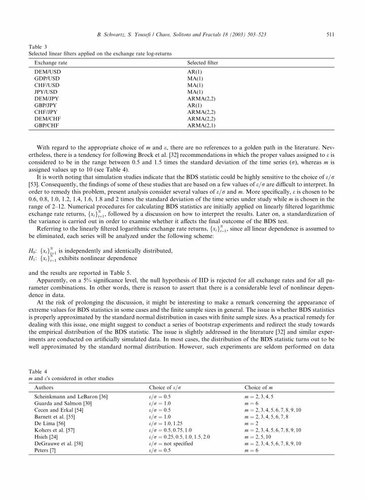
With regard to the appropriate choice of m and e, there are no references to a golden path in the literature. Nev-

ertheless, there is a tendency for following Brock et al. [32] recommendations in which the proper values assigned to e is

considered to be in the range between 0.5 and 1.5 times the standard deviation of the time series (r), whereas m is

assigned values up to 10 (see Table 4).

It is worth noting that simulation studies indicate that the BDS statistic could be highly sensitive to the choice of e=r[53]. Consequently, the findings of some of these studies that are based on a few values of e=r are difficult to interpret. In

order to remedy this problem, present analysis consider several values of e=r and m. More specifically, e is chosen to be

0.6, 0.8, 1.0, 1.2, 1.4, 1.6, 1.8 and 2 times the standard deviation of the time series under study while m is chosen in the

range of 2–12. Numerical procedures for calculating BDS statistics are initially applied on linearly filtered logarithmic

exchange rate returns, fxtgNt¼1, followed by a discussion on how to interpret the results. Later on, a standardization of

the variance is carried out in order to examine whether it affects the final outcome of the BDS test.

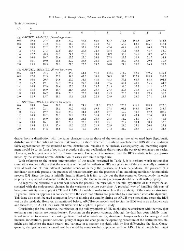
Referring to the linearly filtered logarithmic exchange rate returns, fxtgNt¼1, since all linear dependence is assumed to

be eliminated, each series will be analyzed under the following scheme:

H0: fxtgNt¼1 is independently and identically distributed,

H1: fxtgNt¼1 exhibits nonlinear dependence

and the results are reported in Table 5.

Apparently, on a 5% significance level, the null hypothesis of IID is rejected for all exchange rates and for all pa-

rameter combinations. In other words, there is reason to assert that there is a considerable level of nonlinear depen-

dence in data.

At the risk of prolonging the discussion, it might be interesting to make a remark concerning the appearance of

extreme values for BDS statistics in some cases and the finite sample sizes in general. The issue is whether BDS statistics

is properly approximated by the standard normal distribution in cases with finite sample sizes. As a practical remedy for

dealing with this issue, one might suggest to conduct a series of bootstrap experiments and redirect the study towards

the empirical distribution of the BDS statistic. The issue is slightly addressed in the literature [32] and similar exper-

iments are conducted on artificially simulated data. In most cases, the distribution of the BDS statistic turns out to be

well approximated by the standard normal distribution. However, such experiments are seldom performed on data

Table 4

m and e�s considered in other studies

Authors Choice of e=r Choice of m

Scheinkmann and LeBaron [36] e=r ¼ 0:5 m ¼ 2; 3; 4; 5

Guarda and Salmon [30] e=r ¼ 1:0 m ¼ 6

Cecen and Erkal [54] e=r ¼ 0:5 m ¼ 2; 3; 4; 5; 6; 7; 8; 9; 10

Barnett et al. [55] e=r ¼ 1:0 m ¼ 2; 3; 4; 5; 6; 7; 8

De Lima [56] e=r ¼ 1:0; 1:25 m ¼ 2

Kohers et al. [57] e=r ¼ 0:5; 0:75; 1:0 m ¼ 2; 3; 4; 5; 6; 7; 8; 9; 10

Hsieh [24] e=r ¼ 0:25; 0:5; 1:0; 1:5; 2:0 m ¼ 2; 5; 10

DeGrauwe et al. [58] e=r ¼ not specified m ¼ 2; 3; 4; 5; 6; 7; 8; 9; 10

Peters [7] e=r ¼ 0:5 m ¼ 6

Table 3

Selected linear filters applied on the exchange rate log-returns

Exchange rate Selected filter

DEM/USD AR(1)

GDP/USD MA(1)

CHF/USD MA(1)

JPY/USD MA(1)

DEM/JPY ARMA(2,2)

GBP/JPY AR(1)

CHF/JPY ARMA(2,2)

DEM/CHF ARMA(2,2)

GBP/CHF ARMA(2,1)


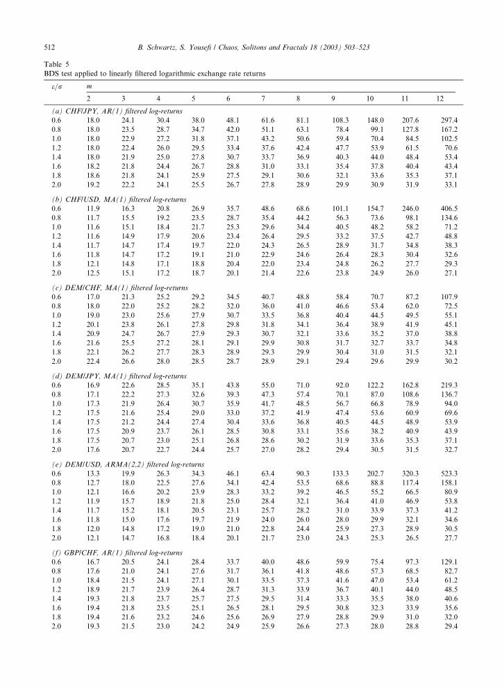
Table 5

BDS test applied to linearly filtered logarithmic exchange rate returns

e=r m

2 3 4 5 6 7 8 9 10 11 12

(a) CHF/JPY, AR(1) filtered log-returns

0.6 18.0 24.1 30.4 38.0 48.1 61.6 81.1 108.3 148.0 207.6 297.4

0.8 18.0 23.5 28.7 34.7 42.0 51.1 63.1 78.4 99.1 127.8 167.2

1.0 18.0 22.9 27.2 31.8 37.1 43.2 50.6 59.4 70.4 84.5 102.5

1.2 18.0 22.4 26.0 29.5 33.4 37.6 42.4 47.7 53.9 61.5 70.6

1.4 18.0 21.9 25.0 27.8 30.7 33.7 36.9 40.3 44.0 48.4 53.4

1.6 18.2 21.8 24.4 26.7 28.8 31.0 33.1 35.4 37.8 40.4 43.4

1.8 18.6 21.8 24.1 25.9 27.5 29.1 30.6 32.1 33.6 35.3 37.1

2.0 19.2 22.2 24.1 25.5 26.7 27.8 28.9 29.9 30.9 31.9 33.1

(b) CHF/USD, MA(1) filtered log-returns

0.6 11.9 16.3 20.8 26.9 35.7 48.6 68.6 101.1 154.7 246.0 406.5

0.8 11.7 15.5 19.2 23.5 28.7 35.4 44.2 56.3 73.6 98.1 134.6

1.0 11.6 15.1 18.4 21.7 25.3 29.6 34.4 40.5 48.2 58.2 71.2

1.2 11.6 14.9 17.9 20.6 23.4 26.4 29.5 33.2 37.5 42.7 48.8

1.4 11.7 14.7 17.4 19.7 22.0 24.3 26.5 28.9 31.7 34.8 38.3

1.6 11.8 14.7 17.2 19.1 21.0 22.9 24.6 26.4 28.3 30.4 32.6

1.8 12.1 14.8 17.1 18.8 20.4 22.0 23.4 24.8 26.2 27.7 29.3

2.0 12.5 15.1 17.2 18.7 20.1 21.4 22.6 23.8 24.9 26.0 27.1

(c) DEM/CHF, MA(1) filtered log-returns

0.6 17.0 21.3 25.2 29.2 34.5 40.7 48.8 58.4 70.7 87.2 107.9

0.8 18.0 22.0 25.2 28.2 32.0 36.0 41.0 46.6 53.4 62.0 72.5

1.0 19.0 23.0 25.6 27.9 30.7 33.5 36.8 40.4 44.5 49.5 55.1

1.2 20.1 23.8 26.1 27.8 29.8 31.8 34.1 36.4 38.9 41.9 45.1

1.4 20.9 24.7 26.7 27.9 29.3 30.7 32.1 33.6 35.2 37.0 38.8

1.6 21.6 25.5 27.2 28.1 29.1 29.9 30.8 31.7 32.7 33.7 34.8

1.8 22.1 26.2 27.7 28.3 28.9 29.3 29.9 30.4 31.0 31.5 32.1

2.0 22.4 26.6 28.0 28.5 28.7 28.9 29.1 29.4 29.6 29.9 30.2

(d) DEM/JPY, MA(1) filtered log-returns

0.6 16.9 22.6 28.5 35.1 43.8 55.0 71.0 92.0 122.2 162.8 219.3

0.8 17.1 22.2 27.3 32.6 39.3 47.3 57.4 70.1 87.0 108.6 136.7

1.0 17.3 21.9 26.4 30.7 35.9 41.7 48.5 56.7 66.8 78.9 94.0

1.2 17.5 21.6 25.4 29.0 33.0 37.2 41.9 47.4 53.6 60.9 69.6

1.4 17.5 21.2 24.4 27.4 30.4 33.6 36.8 40.5 44.5 48.9 53.9

1.6 17.5 20.9 23.7 26.1 28.5 30.8 33.1 35.6 38.2 40.9 43.9

1.8 17.5 20.7 23.0 25.1 26.8 28.6 30.2 31.9 33.6 35.3 37.1

2.0 17.6 20.7 22.7 24.4 25.7 27.0 28.2 29.4 30.5 31.5 32.7

(e) DEM/USD, ARMA(2,2) filtered log-returns

0.6 13.3 19.9 26.3 34.3 46.1 63.4 90.3 133.3 202.7 320.3 523.3

0.8 12.7 18.0 22.5 27.6 34.1 42.4 53.5 68.6 88.8 117.4 158.1

1.0 12.1 16.6 20.2 23.9 28.3 33.2 39.2 46.5 55.2 66.5 80.9

1.2 11.9 15.7 18.9 21.8 25.0 28.4 32.1 36.4 41.0 46.9 53.8

1.4 11.7 15.2 18.1 20.5 23.1 25.7 28.2 31.0 33.9 37.3 41.2

1.6 11.8 15.0 17.6 19.7 21.9 24.0 26.0 28.0 29.9 32.1 34.6

1.8 12.0 14.8 17.2 19.0 21.0 22.8 24.4 25.9 27.3 28.9 30.5

2.0 12.1 14.7 16.8 18.4 20.1 21.7 23.0 24.3 25.3 26.5 27.7

(f) GBP/CHF, AR(1) filtered log-returns

0.6 16.7 20.5 24.1 28.4 33.7 40.0 48.6 59.9 75.4 97.3 129.1

0.8 17.6 21.0 24.1 27.6 31.7 36.1 41.8 48.6 57.3 68.5 82.7

1.0 18.4 21.5 24.1 27.1 30.1 33.5 37.3 41.6 47.0 53.4 61.2

1.2 18.9 21.7 23.9 26.4 28.7 31.3 33.9 36.7 40.1 44.0 48.5

1.4 19.3 21.8 23.7 25.7 27.5 29.5 31.4 33.3 35.5 38.0 40.6

1.6 19.4 21.8 23.5 25.1 26.5 28.1 29.5 30.8 32.3 33.9 35.6

1.8 19.4 21.6 23.2 24.6 25.6 26.9 27.9 28.8 29.9 31.0 32.0

2.0 19.3 21.5 23.0 24.2 24.9 25.9 26.6 27.3 28.0 28.8 29.4


drawn from a distribution with the same characteristics as those of the exchange rate series used here (leptokurtic

distribution with fat tails and moderate skewness). In short, whether it is safe to conclude that BDS statistic is always

fairly approximated by the standard normal distribution, remains to be unclear. Consequently, an interesting experi-

ment would be to perform a bootstrap procedure through replications drawn upon the observed exchange rate series.

However, such experiment is left for future research. For now, it is assumed that the BDS statistic is fairly approxi-

mated by the standard normal distribution in cases with finite sample size.

With reference to the proper interpretation of the results presented in Table 5, it is perhaps worth noting that

simulation studies indicate that the rejection of the null hypothesis of IID in a given set of data is generally consistent

with at least one of four different possible scenarios namely the presence of linear dependence, the presence of a

nonlinear stochastic process, the presence of nonstationarity and the presence of an underlying nonlinear deterministic

process [25]. Since the data is initially linearly filtered, it is fair to rule out the first scenario. Consequently, in order

to present a qualified statement on the last scenario, the two remaining scenarios should be dealt with properly.

As regards the presence of a nonlinear stochastic process, the rejection of the null hypothesis of IID might be as-

sociated with the endogenous changes in the variance structure over time. A practical way of handling this sort of

heteroskedasticity is to apply ARCH and GARCH models in order to explain the instability of the variance structure.

In general, such an approach is consistent with the view that returns are generated by a nonlinear stochastic dynamics.

This issue also might be used to argue in favor of filtering the data by fitting an ARCH-type model and rerun the BDS

test on the residuals. However, as mentioned before, ARCH-type models tend to bias the BDS test in an unknown way

and therefore, no ARCH or GARCH filters will be applied in present study.

Considering the final scenario, the rejection of the null hypothesis of IID might also be consistent with the view that

exchange rate returns are nonstationary. Focusing on the present context, although the data has been initially trans-

ferred in order to remove the most significant part of nonstationarity, structural changes such as technological and

financial innovations, pseudo-seasonal policy changes and changes in the operating procedure of the central banks, etc.

might also influence the mean return and variance in a manner not dealt with by first differencing the data. Conse-

quently, changes in variance need not be caused by some stochastic process such as ARCH type models but might

Table 5 (continued)

e=r m

2 3 4 5 6 7 8 9 10 11 12

(g) GBP/JPY, ARMA(2,2) filtered log-returns

0.6 19.2 24.4 29.9 37.2 47.6 62.0 83.5 116.8 168.3 250.7 384.3

0.8 18.8 23.2 27.2 31.9 38.0 45.0 54.1 66.7 83.1 106.1 138.4

1.0 18.5 22.2 25.3 28.7 32.9 37.3 42.4 48.8 56.7 66.8 79.7

1.2 17.8 21.3 23.8 26.4 29.4 32.3 35.4 39.1 43.5 48.7 55.0

1.4 17.2 20.3 22.5 24.6 26.8 28.9 30.9 33.2 35.7 38.7 42.2

1.6 16.6 19.7 21.6 23.3 25.0 26.4 27.8 29.3 30.9 32.7 34.8

1.8 16.1 19.0 20.8 22.2 23.5 24.6 25.6 26.7 27.8 29.0 30.3

2.0 15.5 18.5 20.1 21.3 22.3 23.2 24.0 24.8 25.5 26.3 27.2

(h) GBP/USD, ARMA(2,2) filtered log-returns

0.6 18.2 25.3 33.9 45.9 64.1 91.8 137.0 214.9 352.9 599.6 1049.4

0.8 17.0 22.3 27.9 34.6 43.5 55.0 70.3 91.5 122.9 168.9 237.2

1.0 16.0 20.5 24.6 29.0 34.6 41.0 48.3 57.1 68.7 84.3 104.4

1.2 15.2 19.1 22.3 25.4 29.3 33.4 37.6 42.4 48.1 55.5 64.2

1.4 14.4 17.9 20.6 23.0 25.9 28.7 31.3 34.0 37.2 41.1 45.5

1.6 13.6 16.9 19.4 21.4 23.6 25.7 27.5 29.3 31.3 33.6 36.2

1.8 13.0 16.2 18.6 20.3 22.2 24.0 25.3 26.6 28.0 29.5 31.2

2.0 12.5 15.7 18.1 19.6 21.3 22.8 23.9 24.9 26.0 27.1 28.3

(i) JPY/USD, ARMA(2,2) filtered log-returns

0.6 18.8 26.4 36.9 51.8 74.8 111.3 171.5 276.2 456.1 768.9 1322.6

0.8 16.7 22.1 28.5 36.2 46.1 59.5 77.8 105.1 143.9 200.3 283.9

1.0 15.5 19.7 24.2 28.9 34.1 40.2 47.7 57.9 70.7 87.2 108.7

1.2 14.8 18.2 21.5 24.6 27.9 31.4 35.1 39.9 45.4 52.0 59.9

1.4 14.1 16.9 19.4 21.8 24.1 26.3 28.5 31.2 34.0 37.3 41.1

1.6 13.8 16.1 18.3 20.2 22.0 23.7 25.1 26.7 28.4 30.3 32.5

1.8 13.4 15.5 17.4 19.0 20.5 21.9 22.9 24.0 25.1 26.4 27.8

2.0 12.8 14.8 16.6 17.9 19.2 20.3 21.2 21.9 22.7 23.6 24.5


emerge exogenously. However, this scenario would be difficult to model without any specific knowledge about the

possible exogenous variables and the underlying dynamics. In our reading, this issue is rarely addressed in other studies

in nonlinear dynamics and econometrics. Nevertheless, Hsieh [24] is among the few contributions in the literature that

suggest a simple procedure for modeling exogenous changes in variance structure. The idea is to assume that time is the

single exogenous variable that is responsible for this sort of exogenous hetereoskedasticity. In order to proceed, it is

further assumed that the exchange rate changes within a month have the same variance and variation occur across

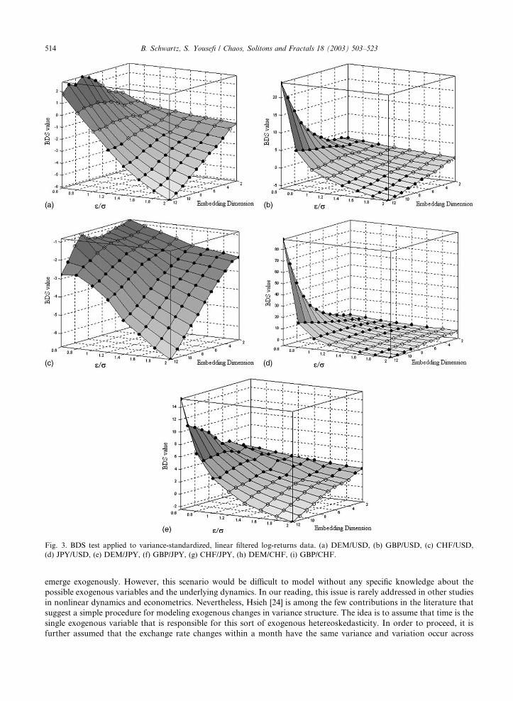
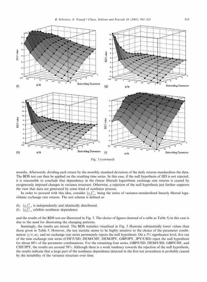
Fig. 3. BDS test applied to variance-standardized, linear filtered log-returns data. (a) DEM/USD, (b) GBP/USD, (c) CHF/USD,

(d) JPY/USD, (e) DEM/JPY, (f) GBP/JPY, (g) CHF/JPY, (h) DEM/CHF, (i) GBP/CHF.


months. Afterwards, dividing each return by the monthly standard deviation of the daily returns standardizes the data.

The BDS test can then be applied on the resulting time series. In this case, if the null hypothesis of IID is not rejected,

it is reasonable to conclude that dependency in the (linear filtered) logarithmic exchange rate returns is caused by

exogenously imposed changes in variance structure. Otherwise, a rejection of the null hypothesis just further supports

the view that data are generated by some kind of nonlinear process.

In order to proceed with this idea, consider fxtgNt¼1 being the series of variance-standardized linearly filtered loga-

rithmic exchange rate returns. The test scheme is defined as

H0: fxtgNt¼1 is independently and identically distributed,

H1: fxtgNt¼1 exhibits nonlinear dependence

and the results of the BDS test are illustrated in Fig. 3. The choice of figures (instead of a table as Table 5) in this case is

due to the need for illustrating the changing patterns.

Seemingly, the results are mixed. The BDS statistics visualized in Fig. 3 illustrate substantially lower values than

those given in Table 5. However, the test statistic seems to be highly sensitive to the choice of the parameter combi-

nation ðe=r;mÞ, and no exchange rate series persistently rejects the null hypothesis. On a 5% significance level, five out

of the nine exchange rate series (CHF/USD, DEM/CHF, DEM/JPY, GBP/JPY, JPY/USD) reject the null hypothesis

for about 60% of the parameter combinations. For the remaining four series, GBP/USD, DEM/USD, GBP/CHF, and

CHF/JPY, the results are around 50%. Although there is a weak tendency towards the rejection of the null hypothesis,

the results indicate that a large part of the nonlinear dependence detected in the first test procedures is probably caused

by the instability of the variance structure over time.

Fig. 3 (continued)


To conclude, the application of BDS procedures provide significant indication of strong dependency among ob-

servations in the nine exchange rate series. The preponderance of evidence, even after accounting for the changing

variance, is in support of rejecting the null hypothesis of IID. Therefore it is fair to infer that the exchange rate series

seem to exhibit a certain degree of nonlinearity. However, in the case of GBP/USD, DEM/USD, GBP/CHF, and CHF/

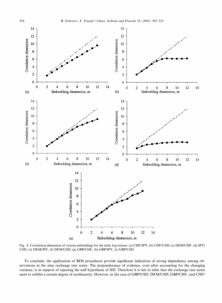
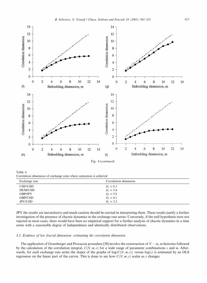
Fig. 4. Correlation dimension of various embeddings for the daily log-returns. (a) CHF/JPY, (b) CHF/USD, (c) DEM/CHF, (d) JPY/

USD, (e) DEM/JPY, (f) DEM/USD, (g) GBP/CHF, (h) GBP/JPY, (i) GBP/USD.


JPY the results are inconclusive and much caution should be exerted in interpreting them. These results justify a further

investigation of the presence of chaotic dynamics in the exchange rate series. Conversely, if the null hypothesis were not

rejected in most cases, there would have been no empirical support for a further analysis of chaotic dynamics in a time

series with a reasonable degree of independence and identically distributed observations.

3.3. Evidence of low fractal dimension: estimating the correlation dimension

The application of Grassberger and Procaccia procedure [38] involve the construction of N � m, m-histories followed

by the calculation of the correlation integral, CðN ;m; eÞ for a wide range of parameter combinations e and m. After-

wards, for each exchange rate series the slopes of the graphs of logðCðN ;m; eÞÞ versus logðeÞ is estimated by an OLS

regression on the linear part of the curves. This is done to see how CðN ;m; eÞ scales as e changes.

Fig. 4 (continued)

Table 6

Correlation dimension of exchange rates where saturation is achieved

Exchange rate Correlation dimension

CHF/USD Dc � 6:1

DEM/USD Dc � 5:4

GBP/JPY Dc � 5:8

GBP/USD Dc � 4:1

JPY/USD Dc � 3:2


As regards the actual choice of parameters e and m, it is worth noting that for each m, a total of 124 different values

of e have been chosen. Consequently, each curve consists of 124 points in the logðeÞ, logðCðN ;m; eÞÞ diagram. The values

of the 124 e�s are not the same for all exchange rates series. Instead, for each series the e�s have been chosen so as to

ensure that both high values of CðN ;m; eÞ (values close to one) and low values of CðN ;m; eÞ (values close to zero) are

reached and a fair graphical representation of each curve is achieved. The embedding dimension has been chosen in the

range of m ¼ 2–12. The results of the calculations are presented in the Fig. 4.

Apparently, the logðeÞ � logðCðN ;m; eÞÞ curves continue to increase with the embedding dimension for some cases,

indicating that there is no clearly distinguishable low-dimensional fractal attractor associated with the underlying

dynamics of the related exchange rate series. In the remaining cases, the saturation is achieved and results of the

estimation procedures are summarized in Table 6.

With regard to GBP/JPY and DEM/USD exchange rates, a plateau of the correlation dimension is barely reached.

In the remaining three exchange rates, a clear saturation is observed. These results indicate that the underlying dy-

namics of these exchange rates are probably associated with a low dimensional attractor. From a theoretical viewpoint

the estimated correlation dimensions are informative on the minimum number of state variables that are needed to

model the dynamics of a given exchange rate.

The proper interpretation of these results requires much caution since the reliability of dimensional algorithms

applied to empirical data is often associated with spurious results that are often leaning towards false identification of

the underlying dynamics (either chaotic or stochastic). Perhaps it is worth the effort to outline a few critical issues that

might interfere in the interpretation of these results.

The first issue is to secure that the low correlation dimension estimates have not been caused by some stochastic

process. A practical remedy to handle this problem is to shuffle the data and rerun the estimation procedure. If the

estimated values remain unchanged, the process is most probably stochastic otherwise deterministic [36]. The second

issue concerns the role of autocorrelation in the data. For instance it is conceivable that stochastic data sets with

autocorrelated observations cause problems since the implementation of the Grassberger–Procaccia algorithm on

temporal correlated observations might lead to abnormal behavior in the correlation integral and the result may be a

spuriously low estimate of the correlation dimension [47]. However, this problem is of minor importance in present

context. Considering the values of the SACFs in present study, there is no reason to believe that autocorrelation should

be a problem in any of the nine exchange rate series considered here. As a result, saturation in the correlation dimension

estimate may be seen as an indication of some sort of determinism in the data. The third issue concerns the implications

of insufficient reconstruction of the phase space and insufficient number of observations. The limited number of em-

bedding dimensions that are usually considered (for instance 2–12 in present study) might be insufficient for reaching

saturation in the graphical procedures that is mentioned before. In this case an underlying chaotic process cannot be

ruled out, since the dimension of the attractor may be too large to be properly recovered within an embedded phase

space with a relatively small embedding dimension. On the other hand, the lack of saturation in the correlation di-

mension may also be due to insufficient lengths of the data sets. The Grassberger and Procaccia procedure relies on the

assumption that the data set is of infinite length. Only then it is expected that the estimates of the correlation dimension

converge to the dimension of the chaotic attractor. However, in empirical studies, one needs to have an idea about the

minimum number of data points Nmin that is needed for estimating the dimension of an attractor of dimension D.

Eckmann and Ruelle [49] suggest that Nmin > 10ðD=2Þðlogð1=qÞÞ where q ¼ e=r, e is the same as noted before, r is the di-

ameter of the reconstructed attractor and q is usually taken to be around 0.1. Consequently, it can be seen that with a

dataset of approximately 6.500 observations, no dimension estimates higher than approximately 7 or 8 can be obtained.

This might be the reason why for some series the saturation is not achieved. In present context, whether a time series

of approximately 7000 observations is to be regarded as a small dataset is difficult to asses.

The fourth issue concerns the presence of noise in data that might influence the estimation procedure. Whether the

noise is an inherent element of the underlying dynamics or it is a manifestation of the measurement error, the task of

handling noise in estimating the correlation dimension remains to be difficult. In general, it is possible to apply noise

reduction procedures on the data but then the process of filtering itself may introduce potential correlations that might

lead to a low correlation dimension where no chaos would normally be present [47]. The fifth issue concerns the re-

liability of the Grassberger–Procaccia algorithm as a mean of detecting low-dimensional chaos. From a theoretical

point of view, Brock [39] shows that the correlation integral is independent of the choice of norm. From a practical

point of view, Kugiumtzis [40] shows how different norms may lead to different results in the estimation of the cor-

relation dimension when observations include additive noise. Since the Euclidian norm seems to be the most reliable

norm in the presence of additive noise [40], this norm has been used here to generate estimates of the correlation

dimension.

To conclude, one should interpret the estimates of the correlation dimension with much caution since there are

several possible reasons for the presence (or lack) of conclusive evidence of a low fractal dimension involved in such


analysis. Noise, insufficient data length, or a high (yet finite) correlation dimension are among potential factors that

may fool the researcher into believing that there is no underlying deterministic component in the data when there

actually is (or vice versa).

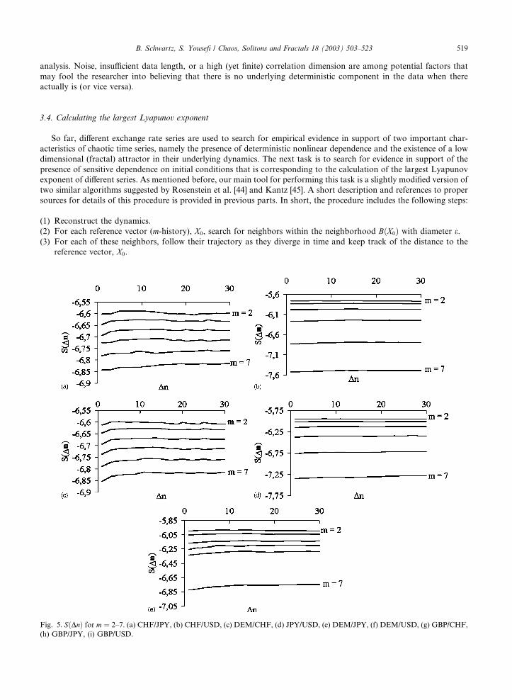
3.4. Calculating the largest Lyapunov exponent

So far, different exchange rate series are used to search for empirical evidence in support of two important char-

acteristics of chaotic time series, namely the presence of deterministic nonlinear dependence and the existence of a low

dimensional (fractal) attractor in their underlying dynamics. The next task is to search for evidence in support of the

presence of sensitive dependence on initial conditions that is corresponding to the calculation of the largest Lyapunov

exponent of different series. As mentioned before, our main tool for performing this task is a slightly modified version of

two similar algorithms suggested by Rosenstein et al. [44] and Kantz [45]. A short description and references to proper

sources for details of this procedure is provided in previous parts. In short, the procedure includes the following steps:

(1) Reconstruct the dynamics.

(2) For each reference vector (m-history), X0, search for neighbors within the neighborhood BðX0Þ with diameter e.(3) For each of these neighbors, follow their trajectory as they diverge in time and keep track of the distance to the

reference vector, X0.

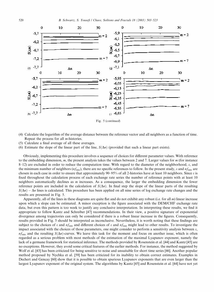
Fig. 5. SðDnÞ for m ¼ 2–7. (a) CHF/JPY, (b) CHF/USD, (c) DEM/CHF, (d) JPY/USD, (e) DEM/JPY, (f) DEM/USD, (g) GBP/CHF,

(h) GBP/JPY, (i) GBP/USD.


(4) Calculate the logarithm of the average distance between the reference vector and all neighbors as a function of time.

Repeat the process for all m-histories.

(5) Calculate a final average of all these averages.

(6) Estimate the slope of the linear part of the line, SðDnÞ (provided that such a linear part exists).

Obviously, implementing this procedure involves a sequence of choices for different parameter values. With reference

to the embedding dimension, m, the present analysis takes the values between 2 and 7. Larger values for m (for instance

8–12) are excluded in order to reduce the computation time. With regard to the diameter of the neighborhood, e, and

the minimum number of neighbors (nfmin), there are no specific references to follow. In the present study, e and nfmin are

chosen in each case in order to ensure that approximately 90–95% of all 2-histories have at least 10 neighbors. Since e is

fixed throughout the calculation process of each exchange rate series the number of reference points with at least 10

neighbors automatically declines as m increases. As a consequence, the larger the embedding dimension the fewer

reference points are included in the calculation of SðDnÞ. In final step the slope of the linear parts of the resulting

SðDnÞ � Dn lines is calculated. This procedure has been applied on all nine series of log exchange rate changes and the

results are presented in Fig. 5.

Apparently, all of the lines in these diagrams are quite flat and do not exhibit any robust (i.e. for all m) linear increase

upon which a slope can be estimated. A minor exception is the figure associated with the DEM/CHF exchange rate

data, but even this pattern is too week to justify any conclusive interpretation. In interpreting these results, we find it

appropriate to follow Kantz and Schreiber [47] recommendations. In their view, a positive signature of exponential

divergence among trajectories can only be considered if there is a robust linear increase in the figures. Consequently,

results provided in Fig. 5 should be interpreted as inconclusive. Nevertheless, it is worth noting that these findings are

subject to the choices of e and nfmin and different choices of e and nfmin might lead to other results. To investigate the

impact associated with the choices of those parameters, one might consider to perform a sensitivity analysis between e,nfmin and the resulting SðDnÞ-curves. We leave this task for the moment and focus on another issue, which is often

regarded as a serious problem with most methods of the estimation of the maximal Lyapunov exponent, namely the

lack of a germane framework for statistical inference. The methods provided by Rosenstein et al. [44] and Kantz [45] are

no exceptions. However, they avoid some critical features of the earlier methods. For instance, the method suggested by

Wolf et al. [43] has been criticized for being sensitive to noise and unsuitable for short time series [46]. Another popular

method proposed by Nychka et al. [59] has been criticized for its inability to obtain correct estimates. Examples in

Dechert and Gencay [60] show that it is possible to obtain spurious Lyapunov exponents that are even larger than the

largest Lyapunov exponent of the original system. The algorithms by Kantz [45] and Rosenstein et al. [44] have not yet

Fig. 5 (continued)


been subject to similar criticism. Therefore, it is fair to assume that their procedures are the best available instruments

for the time being. That is the main reason why we have been reluctant to apply other methods in order to crosscheck

the obtained results.

4. Conclusions

Evidently, it should be clear that proving chaotic dynamic in real systems is a futile and impossible task [61].

Nevertheless, empirical studies of univariate time series have been in many cases redirected towards a general search for

empirical evidence and meaningful indication in support of the presence of chaotic dynamics in economic and financial

data. Challenging the underlying reasoning behind the theory of efficient markets have been among the major themes in

these studies. The main intention of present study has been to contribute to this body of literature by elaborating on

some new perspectives on how a constructive contribution to this debate should be associated with a clearly defined

working hypothesis, a sequence of coherent procedures for the empirical investigation, relevant reflections on the

possible limitations of these procedures and finally an effort to fit the entire analysis into a larger picture associated

with the previous contributions to the literature.

In order to proceed, nine very long exchange rate series have been chosen for the analysis. These series included the five

most traded currencies and cover almost the whole period after the breakdown of the Bretton Woods system. Significant

efforts have been exerted in order to define a working hypothesis and address three important features of chaotic time

series, namely the presence of nonlinear dependence, the existence of a low dimensional (fractal) attractor in their un-

derlying dynamics and finally the search for indication of the presence of sensitive dependence on initial conditions.

The BDS test procedure was initially applied to the linearly filtered logarithmic exchange rate returns and the ev-

idence of nonlinear dependence among observations was established in all nine series. However, a standardization of

the variance in each series lowered the significance of the test statistics. On a 5% significance level, approximately 50%

of the test statistics now lead to acceptance of the null hypothesis of IID.

In the next stage the series were investigated for signs of a low correlation dimension (a lower estimate of the fractal

dimension) in the underlying dynamics. The results were mixed and evidence pointing in the direction of a low fractal

dimension was established in the case of the CHF/USD, DEM/USD, GBP/JPY, GBP/USD and JPY/USD exchange

rate return series.

Finally, the series were investigated for the presence of sensitive dependence on initial conditions since such a

property implies the existence of a positive maximal Lyapunov exponent [32]. A slightly modified version of the method

by Rosenstein et al. [44] and Kantz [45] was chosen to estimate the largest Lyapunov exponent. The results were in-

conclusive and could not be pointed in the direction of a positive maximal Lyapunov exponent.

To summarize, the first property was fulfilled by all exchange rate series although caution should be exerted in

interpreting results on GBP/USD, DEM/USD, GBP/CHF, and CHF/JPY exchange rate series. The second property

was fulfilled for the series GBP/USD, DEM/USD, CHF/USD, GBP/JPY, and JPY/USD. Finally, none of the exchange

rate-return series fulfilled the third property (sensitive dependence). Thus, no series satisfied all three main indications of

the presence of chaos. However, it is recognized that the results are dependent on the methods used, a proper recon-

struction of the dynamics, interpretation of the graphs, degree of noise in data, and a range of other methodological

issues involved in the analysis.

The unique features and specific contributions of present efforts are the results of the following steps. First, the analysis

of chaos in observed data has been performed on quite long time series (of daily data) that almost include the whole period

of floating exchange rate system. In our reading of other studies in nonlinear dynamics and econometrics, there are no

other similar studies with the same magnitude of the analyzed data that also span over 1970s, 1980s and 1990s.

Second, to the best of our knowledge, only a few published papers have jointly applied the BDS test, the correlation

dimension test, and the test for a positive maximal Lyapunov exponent. Therefore, it is fair to state that present study

contributes to an overall picture of the role on chaos in exchange rate dynamics that has not been seen before.

As regards the BDS statistics, the test is applied for 88 combinations of the embedding dimension m and e. A glance

at the literature reveals that usually much fewer combinations are considered. But in our view applying this procedure

on a range of different combinations provides a more reliable platform to find out that whether the results are

depending on the choice of e and m or not.

As regards the issue of exponential divergence of nearby trajectories, a slightly modified version of the method,

proposed by Rosenstein et al. [44] and Kantz [45], has been discussed and implemented in order to conduct a search for

a positive estimate of the maximum Lyapunov exponent. Other studies concerned with the estimation of Lyapunov

exponents from time series usually consider the methods by Wolf et al. [43] or Nychka et al. [59]. However, these

methods have been challenged on various grounds over the years [46,60].


We would like to conclude by outlining a series of promising themes for future research that have been uncovered

during the present analysis. Most of these features are concerned with the robustness of the empirical findings. The first

issue concerns the study of impacts of political and social changes on the overall procedures. The standardization

procedure performed in connection with the BDS test suggests that the rejection of the null hypothesis is significantly

related to the unstable variance structure. The instability in variance structure might be associated with the emergence

of new political and social conditions such as the ever increasing number of floating currencies since 1970s, the

emergence of significant and persistent trade imbalances among major economies in 1980s and the growing interde-

pendencies among world economies as a consequence of rapid globalization in 1990s. A feasible approach for dealing

with these sorts of impacts is to track down major events, divide the time series into regions of stability and repeat the

BDS test on each series.

The second issue concerns the role of noise in the measurement process and its impact on empirical procedures.

Perhaps the results obtained here would have been different if a noise reduction procedure has been initially applied on

the all series. A good starting point would be the noise reduction algorithms presented in Kantz and Schreiber [47].

Finally, this study may serve as a preliminary justification to test for the predictability of the series associated with a

low correlation dimension (as reported here). In theory, a low correlation dimension signifies the existence of predictive

patterns in the exchange rate market. Therefore, by using methods especially developed to exploit the existence of a low

fractal dimension one should (in theory) be able to outperform the market. Some of these methods can be found in

Kantz and Schreiber [47].

References

[1] Campbell JY, Lo AW, MacKinalay AC. The econometrics of financial markets. Princeton University Press; 1997.

[2] LeBaron B. Technical trading rule profitability and foreign exchange intervention. J Int Econ 1999;49:125–43.

[3] Mandelbrot BB. Fractals and scaling in finance. Springer Verlag; 1997.

[4] Gencay R, Stengos T. Technical trading rules and the size of the risk premium in security returns. Stud Nonlinear Dyn Econom

1997;2:23–34.

[5] Trippi RR, editor. Chaos and nonlinear dynamics in the financial markets. Irwin Professional Publishing; 1995.

[6] Peters EE. Chaos and order in the capital markets. Wiley and Sons; 1991.

[7] Peters EE. Fractal market analysis. Wiley and Sons; 1994.

[8] Brock WA, Lakonishok J, LeBaron B. Simple technical rules and the stochastic properties of stock returns. J Finance

1992;XLVII(5):1731–64.

[9] Patterson K. An introduction to applied econometrics: a time series approach. Palgrave, 2000.

[10] Endres W. Applied econometric time series. Wiley series in probability and mathematical statistics, 1995.

[11] Hinich M, Patterson D. Evidence of nonlinearity in daily stocks return. J Business Econ Statist 1985;3:69–76.

[12] Brillinger D. An introduction to polyspectrum. Ann Math Stat 1965;36:1351–74.

[13] Rao TS, Gabr M. A test for linearity of stationary time series analysis. J Time Ser Anal 1980;1:145–58.

[14] Hinich M. Testing for gaussianity and linearity of a stationary time series. J Time Ser Anal 1982;3:169–76.

[15] Dunis Ch, Feeny M, editors. Exchange rate forecasting. Woodhead–Faulkner; 1989.

[16] Hsieh D. Statistical properties of daily exchange rates. J Int Econ 1988;24:129–45.

[17] Mees RA, Rogoff K. Empirical exchanges models of the seventies: do they fit out of sample? J Int Econ 1983;14:3–24.

[18] McFarland JW, Pettit RR, Sung SK. The distribution of foreign exchange price changes. J Finance 1982;37:693–715.

[19] Mussa ML. Empirical regularities in the behavior of exchange rates and theories of the foreign exchange markets. In: Bruner K,

Metzler A, editors. Policies for employment, prices and exchange rates, Carnegie-Rochester Conference 11, Amsterdam: North

Holland; 1979.

[20] Cornell WB, Dietrich JK. The efficiency of the foreign exchange markets under floating exchange rates. Rev Econ Statist

1978;60:111–20.

[21] DeGrauwe P, DeWachter H. A chaotic model of the exchange rate: the role of fundamentalists and chartists. Open Econ Rev

1993;4:351–79.

[22] Bajo-Rubio OF, Rodriguez FF, Rivera SS. Chaotic behaviour in exchange rate series. Econ Lett 1992;39:207–11.

[23] Mees R, Rose A. Nonlinear, nonparametric, nonessential exchange rate estimation. AER 1990;80:192–6.

[24] Hsieh D. Testing for nonlinearity in daily foreign exchange rates. J Business 1989;62:339–68.

[25] Hsieh D. Chaos and nonlinear dynamics: application to finance. J Finance 1991;46:1839–77.

[26] Bask M. A positive Lyapunov exponent in Swedish exchange rates? Chaos, Solitons & Fractals 2002; forthcoming.

[27] Bask M. Dimensions and Lyapunov exponents from exchange rate series. Chaos, Solitons & Fractals 1996;7:2199–214.

[28] Bask M, Genacy R. Testing chaotic dynamics via Lyapunov exponents. Physica D 1998;114:l–2.

[29] Serletis A, Gogas P. Chaos in East European black market exchange rates. Res Econ 1997;51:359–85.

[30] Guarda P, Salmon M. On the detection of nonlinearity in foreign exchange data. In: Barnett William A, Kirman Alan P, Salmon

Mark, editors. Nonlinear dynamics and economics. Cambridge: Cambridge University Press; 1995.


[31] Peters EE. A chaotic attractor for S&P 500. Finance Anal J 1991;47(2):55–62.

[32] Brock WA, Hsieh D, LeBaron B. Nonlinear dynamics, chaos and instability: theory and evidence. MIT Press; 1991.

[33] Takens F. Detecting strange attractors in turbulence. In: Rand DA, Young LS, editors. Proceedings of the Symposion on

Dynamical Systems and Turbulence, University of Warwick, 1979–1980. Springer, 1981.

[34] Packard NH, Crutchfield JP, Farmer JD, Shaw RS. Geometry from a time series. Phys Rev Lett 1980;45:712–6.

[35] Liu T, Granger CWJ, Heller WP. Using the correlation exponent to decide whether an economic series is chaotic. J Appl Econom

1992;7:525–39.

[36] Scheinkman JA, LeBaron B. Nonlinear dynamics and stock returns. J Business 1989;62:311–37.

[37] Ding M, Grebogi C, Ott E, Sauer T, Yorke JA. Estimating correlation dimension from a chaotic time series: when does plateau

onset occur. Physica D 1993;69:404–24.

[38] Grassberger P, Procaccia I. Measuring the strangeness of strange attractors. Physica D 1983;9:189–208.

[39] Brock WA. Distinguishing random and deterministic systems. JET 1986;40(1):68–195.

[40] Kugiumtzis D. Assessing different norms in nonlinear analysis of noisy time series. Physica D 1997;105:62–78.

[41] Brock WA, Dechert D, Scheinkmann J, LeBaron B. A test for independence based upon the correlation dimension. Econom Rev

1996;15(3):197–235.

[42] Bollerslev T. Generalized autoregressive conditional heteroscedasticity. J Econom 1986;31:307–27.

[43] Wolf A, Swift JB, Swinney HL, Vastano JA. Determining Lyapunov exponents from a time series. Physica D 1985;16:285–317.

[44] Rosenstein MT, Collins JJ, De Luca CJ. A practical method for calculating largest Lyapunov exponents from small data sets.

Physica D 1993;65:117–34.

[45] Kantz H. A robust method to estimate the maximal Lyapunov exponent of a time series. Phys Lett A 1994;185:77–87.

[46] Brock WA, Sayers C. Is the business cycle characterized by deterministic chaos?. J Mont Econ 1988;22:71–90.

[47] Kantz H, Schreiber T. Nonlinear time series analysis. Cambridge University Press; 1997.

[48] Gilmore CG. A new test for chaos. JEBO 1993;22(2):209–37.

[49] Eckmann JP, Ruelle D. Fundamental limitations for estimating dimension and Lyapunov exponents in dynamical systems.

Physica D 1992;56:185–7.

[50] Vilasuso JR, Cunningham S. Tests for nonlinearity in EMS exchange rates. Stud Nonlinear Dyn Econom 1996;1:155–68.

[51] Fama EF. Efficient capital markets: a review of theory and empirical work. J Finance 1970;25:384–433.

[52] Greene WH. Econometric analysis. Prentice-Hall; 1997.

[53] Kanzler L. Very fast and correctly sized estimation of the BDS statistic. Research Paper. Department of Economics, University of

Oxford; 1999.

[54] Cecen A, Erkal C. Distinguishing between stochastic and deterministic behavior in foreign exchange rate returns: further evidence.

Econ Lett 1996;51(3):323–9.

[55] Barnett WA, Medio A, Serletis A. An experimental design to compare tests of nonlinearity and chaos. In: Barnett William A,

Kirman Alan P, Salmon Mark, editors. Nonlinear dynamics and economics. Cambridge University Press; 1996.

[56] De Lima P. Nuisance parameter free properties of correlation integral based statistics. Econom Rev 1996;15(3):237–59.

[57] Kohers T, Pandey V, Kohers G. Using nonlinear dynamics to test for market efficiency among the major U.S. stock exchanges.

Quart Rev Econ Fin 1997;37(2):523–45.

[58] DeGrauwe P, Dewachter H, Embrechts M. Exchange rate theory chaotic models, foreign exchange markets. Blackwell Publishers;

1993.

[59] Nychka D, Ellner S, Galant AR, McCaffrey D. Estimating Lyapunov exponents with nonparametric regression. J Am Stat Assoc

1992;87:682–95.

[60] Dechert WD, Gencay R. The identification of spurious Lyapunov exponents in Jacobian algorithms. Stud Nonlinear Dyn

Econom 1996;l(3):145–54.

[61] Urbach R. Footprints of chaos in the markets. Prentice Hall; 2000.


Documents

On complex behavior and exchange rate dynamics