On a Nonlinear Transaction-Cost Model for Stock Prices in ...einspem.upm.edu.my/journal/fullpaper/vol11/7. odeki.pdf · Edeki,S.O.,Ugbebor,O.O.andOwoloko,E.A. 1. Introduction Inaprofessionalsetting,theterm‘liquidity’describestheleveltowhichan

Malaysian Journal of Mathematical Sciences 11(1): 83 – 96 (2017)

MALAYSIAN JOURNAL OF MATHEMATICAL SCIENCES

Journal homepage: http://einspem.upm.edu.my/journal

On a Nonlinear Transaction-Cost Model forStock Prices in an Illiquid Market Driven by a

Relaxed Black-Scholes Model Assumptions

S. O. Edeki ∗1, O.O. Ugbebor1,2, and E.A. Owoloko1

1Department of Mathematics, Covenant University, Nigeria2Department of Mathematics, University of Ibadan, Nigeria

E-mail: [email protected]∗Corresponding author

Received: 9th May 2016Accepted: 9th December 2016

ABSTRACT

In an illiquid market, assets cannot be easily sold or exchanged for cashwithout a loss of value (even if it is minimal), this may be due to un-certainty such as transaction cost, lack of interested buyers and so on.This paper considers a nonlinear transaction-cost model for stock pricesin an illiquid market. This nonlinear model surfaced when the constantvolatility assumption of the famous linear Black-Scholes option valuationand pricing model is relaxed via the inclusion of transaction cost. Weobtain approximate solutions to this nonlinear model using the projecteddifferential transform technique or method (PDTM) as a semi-analyticalmethod. The results are very interesting, agree with the associated exactsolutions of Esekon (2013) and that of Gonzalez-Gaxiola et al. (2015).

Keywords: Nonlinear Black-Scholes model, illiquid market, option pric-ing, PDTM.

Edeki, S. O., Ugbebor, O. O. and Owoloko, E. A.

1. Introduction

In a professional setting, the term ‘liquidity’ describes the level to which anunderlying asset can be quickly exercised- sold or bought in the market with theasset’s price not affected. That is to say, that liquidity of an asset describes theflexibility and ease of the asset in terms of quick sales, with less regard to theasset’s price reduction (Acharya and Pedersen (2005);Amihud and Mendelson(1986)). Examples of liquid assets include money or cash as it can be sold foritems such as goods and services (immediately) without (or with minimal) lossof value. A liquid market is basically characterized by ever ready and willinginvestors. On the other hand (Keynes (1971)), in an illiquid market, assetscannot be easily sold or exchanged cash-wise without a noticeable reductionin price due to uncertainty such as transaction cost, lack of interested buyers,among others. In the period of market chaos when the ratio of buyers to sellersis relative not balanced, illiquid type of assets attract higher risks than liquidtypes. Stock option is an example of an illiquid asset.

In the study of modern finance and pricing theory, the standard Black-Scholes model appear very useful (Black and Scholes (1973)). Though, most ofthe assumptions under which this classical arbitrage pricing theory is formu-lated seem not realistic in practice. These include: the asset price or the under-lying asset following a Geometric Brownian Motion (GBM), the drift parameterand the volatility rate are assumed constants, lack of arbitrage opportunities(no risk-free profit), frictionless and competitive markets (Gonzalez-Gaxiolaet al. (2015) and Owoloko and Okeke (2014)). In a competitive market, thereare no transaction costs (say taxes), and trade restrictions are not honoured(say short sale constraints) (Cetin et al. (2004)), while in a competitive market,a trader is free to purchase or sell any amount of a security without alteringthe prices.

Based on the above assumptions, the price of the stock S, at time t (0 < t < T )follows the stochastic differential equation (SDE):

dS = S (µdt+ σdWt) (1)

where µ, σ and Wt are mean rate of return of S, the volatility, and a standardBrownian motion respectively.

For an option value u = u(s, t), we have:

∂u

∂t+ rS

∂u

∂S+

1

2S2σ2 ∂

2u

∂S2− ru = 0 (2)

with u (0, t) = 0, u (s, t) → 0 as S −→ ∞ u (s, T ) = max (S − E, 0) , E is aconstant.

A good number of models with respect to volatility have been proposed inliterature for option pricing. The simplest of them assumes constant volatility.However, it is obvious that constant volatility cannot fully explain observed

84 Malaysian Journal of Mathematical Sciences

On a Nonlinear Transaction-Cost Model for Stock Prices in an Illiquid Market Driven by aRelaxed Black-Scholes Model Assumptions

market prices for options valuation unless when modified (Edeki et al. (2016a);Barles and Soner (1998); Edeki et al. (2016b); Boyle and Vorst (1992)). Equa-tion 1 is a linear partial differential equation (the classical Black-Scholes model).Many researchers have attempted solving equation 2 for analytical or approxi-mate solutions using direct, analytical or semi-analytical methods (Ankudinovaand Ehrhardt (2008); Allahviranloo and Behzadi (2013); Jdar et al. (2005); Ro-drigo and Mamon (2006); Bohner and Zheng (2009); Company et al. (2008);Cen and Le (2011);Edeki et al. (2015)). On relaxing the frictionless and thecompetitive markets’ assumptions, the notion of liquidity is therefore intro-duced, giving rise to a nonlinear version of the Black-Scholes model (as a resultof transaction cost involvement). Bakstein and Howison (2003) referred to liq-uidity as the act of grouping individual trader’s transaction cost in line withthe effect of price slippage. It is therefore, our intention to obtain an analyticalsolution of the nonlinear transaction cost-model for stock prices in an illiquidmarket.

2. The Nonlinear Black-Scholes model(Bakstein and Howison equation)

Here, we will consider a case where both the drift µ , and the volatility σ ,parameters can be expressed as functions of the following: time τ , stock priceS , and the differential coefficients of the option price V . In particular, thatof non-constant modified function:

σ = σ̂

(τ, S,

∂V

∂S,∂2V

∂S2

)(3)

is to be considered. So, (1) becomes:

∂V

∂τ+ rS

∂V

∂S+

1

2S2σ̂2

(τ, S.

∂V

∂S,∂2V

∂S2

)∂2V

∂S2− rV = 0 (4)

Note: the model equation 2 can be improved using (Equation 3) from theaspect of transaction costs inclusion, large trader and illiquid markets effect.In this regard, we will follows the approach of Frey and Patie (2002) and Freyand Stremme (1997) for the effects on the price with the result:

σ = σ̂

(τ, S,

∂V

∂S,∂2V

∂S2

)(1− ρSλ (S)

∂2V

∂S2

)(5)

where σ is the traditional volatility, ρ is a constant measuring the liquidity ofthe market and λ is the price of risk.

Following the assumption that the price of risk is unity (a special case whereλ (S) = 1 , and a little algebra with the notion that:

1 ≈ ((1− f∗)2 (1 + 2f∗ +O(f∗)

3).

Malaysian Journal of Mathematical Sciences 85


We can therefore write 4:

∂V

∂τ+ rS

∂V

∂S+

1

2S2

[σ2

(1 + 2ρS

∂2V

∂S2

)]∂2V

∂S2− rV = 0 (6)

such that V (S, T ) = h(S), S ∈ [0,∞). For the translation t+ τ = T and usingw(S, t) = V (S, τ), equation 6 becomes:

∂w

∂t+ rS

∂w

∂S=

1

2S2σ2

(1 + 2ρS

∂2w

∂S2

)∂2w

∂S2− rw = 0, w(S, 0) = h(S) (7)

Equation7 has an exact solution (Esekon (2013)) of the form:

w(S, t) = w = S−ρ−1√S0

(√Sexp

(r + σ2

4

2

)t+

√S0

4exp

(r +

σ2

4

)t

)(8)

For σ, S0, S, ρ > 0) while r, t ≥ 0, S0 as an initial stock price, with

w(S, 0) = max

(S − ρ−1

(√S0S +

S0

4

), 0

)(9)

Remark: We note here that forρ = 0 , equation 2 is obtained. Existence anduniqueness of this nonlinear model has been established in Liu and Yong (2005).

3. The Overview of the PDT Method

Here, an outline of the modified form of the DTM known as PDTM willbe presented (Jang (2010); Edeki et al. (2016c); Ravi Kanth and Aruna (2012)and Keskin et al. (2011)).

3.1 A note on some basic theorems of the PDTM

In consideration, let u(x, t) be an analytic function at (x∗, t∗) defined on adomain D∗ , so considering the expansion of u(x, t) in Taylor series form, wegive regard to some variables Sv = t , unlike the approach in the classical DTMwhere all the variables are considered. So, the PDTM of u(x, t) with respectto t at t∗ is defined and denoted as follows:

U(x, h) =1

h!

[∂hu (x, t)

∂th

]t=t∗

(10)

such that

u(x, h) =

∞∑h=0

U(x, h)(t− t∗)h (11)



where equation 11 is called an inverse projected differential transform (IPDT)of U(x, h) with respect to(time parameter).

3.1.1 Some Basic Properties and theorems of the PDTM.

a: Ifm(x, t) = αma(x, t)+βmb(x, t), thenM(x, h̄) = αMa(x, h̄)+βMb(x, h̄)

b: If m(x, t) = α∂nm∗(x, t)

∂tn, then m(x, h̄) = α

(h̄+ n)!

h̄!M∗(x, h̄+ n)

c: If m(x, t) = α∂M∗(x, t)

∂t, then M(x, h̄) =

α(h̄+ 1)!M∗(x, h̄+ 1)

h̄!

d: If m(x, t) = ϑ(x)∂nm∗(x, t)

∂xn, then M(x, h̄) = ϑ(x)

∂nM∗(x, h̄)

∂xn

e: If m(x, t) = ϑ(x)m2(x, t), then M(x, h̄) = ϑ(x)

h̄∑r=0

M∗(x, r)M∗(x, h̄− r)

f: If p(x, y) = xryr∗, then P (k, h̄) = δ(k − r, h̄− r∗) = δ(k − r)δ(h̄− r∗)

where

δ(k − r) =

{1, if k = r0, if k 6= r

& δ(k − r∗) =

{1, if k = r∗

0, if k 6= r∗

Thus,

u(x, t) =

∞∑h̄=0

U(x, h̄)th̄ (12)

4. The PDTM and the Nonlinear Model

In this subsection, the PDTM approach will be applied to the model equa-tion 7 as follows:

∂w

∂t= −rS ∂w

∂S− 1

2S2σ2

(1 + 2ρS

∂2w

∂S2

)∂2w

∂S2+ rw (13)

subject to: w(S, 0) = max

(S − ρ−1

(√S0S +

S0

4

), 0

)

∂w

∂t= −

(rS∂w

∂S+

1

2S2σ2

(∂2w

∂S2+ 2ρS

(∂2w

∂S2

)2)− rw

)(14)



At projection, the transformation of equation 14 using PDTM yields:

(k + 1)Wk+1(S) = −(rSW ′k(S) +

1

2S2σ2H − rWk(S)

), (15)

where

H =

(W′′

k (S) + 2ρS

k∑n=0

W′′

n (S)W′′

k−n(S)

)(16)

We write equation 15 for Wk+1 = Wk+1(S) as:

Wk+1 =−1

k + 1

(rSW ′k +

1

2S2σ2

(W′′

k + 2ρS

k∑n=0

W′′

nW′′

k−n

)− rWk

)(17)

subject to : W0 = max

(S − ρ−1

(√S0S +

S0

4

), 0

)(18)

when k = 0.

W1 = −(rSW ′0 +

1

2S2σ2(W

′′

0 + 2ρSW′′

0 W′′

0 )− rW0

)(19)

when k = 1,

W2 = −12

(rSW ′1 + 1

2S2σ2

(W′′

1 + 2ρS∑1n=0W

′′

nW′′

1−n

)− rW1

)= −1

2

(rSW ′1 + 1

2S2σ2(W

′′

1 + 2ρS(W′′

0 W′′

1 +W′′

1 W′′

0 ))− rW1

)(20)

when k = 2,

W3 =−1

3

(rSW ′2 +

1

2S2σ2

(W′′

2 + 2ρS

2∑n=0

W′′

nW′′

2−n

)− rW2

)(21)

when k = 3,

W4 =−1

4

(rSW ′3 +

1

2S2σ2

(W′′

3 + 2ρS

3∑n=0

W′′

nW′′

3−n

)− rW3

)(22)

when k = 4.

W5 =−1

5

(rSW ′4 +

1

2S2σ2

(W′′

4 + 2ρS

4∑n=0

W′′

nW′′

4−n

)− rW4

)(23)



4.1 Numerical Illustration

We recall (8) and (9) as follows;

w(S, t) = w = S − ρ−1√S0

(√Sexp

(r + σ2

4

2

)t+

√S0

4exp

(r +

σ2

4

)t

)(24)

w(S, 0) = max

(S − ρ−1

(√S0S +

S0

4

), 0

)(25)

For numerical computation, the following cases will be considered:

Case I: For r = 0, ρ = −0.01, σ = 0.4, S0 = 4 we thus have the exact solutionand initial condition as:

w(S, t) =S + 200

(√Sexp

(t

50

)+

1

2exp

(t

100

))(26)

w(S, 0) =S + 200√S + 100 (27)

So, applying the PDTM with the parameters in case I through (17)-(23)gives the following:

W (S, 0) = S + 200√S + 100 (28)

W (S, 1) = − S25

(−50

S32

− 50

S2

)(29)

W (S, 2) =− S2

25

(− 8

25

(−50

S32

− 50

S2

)(75

S52

+100

S3

)− 4S

25

(75

S52

+100

S3

)2

− 4S

25

(−50

S32

− 50

S2

)(−375

2S72

+300

S4

)

− S

50

−50

(−425

(75

S52

+ 100S3

)2

− 425

(−50

S32− 50

S2

)(−375

2S72− 300

S4

)S

32

− 1

S32

(50

(− 8

25

(−50

S32

− 50

S2

)(75

S52

+100

S3

)− 4S

25

(75

S52

+100

S3

)2

−4S

25

(−50

S32

− 50

S2

)(−375

2S72

+300

S4

)))))



whence,

w(S, t) =

∞∑h=0

W (S, h)th

=W (S, 0) +W (S, 1)t+W (S, 2)t2 +W (S, h)t3 + · · ·

=(S + 200

√S + 100

)− S

25

(−50

S32

− 50

S2

)t

+

(−S

2

25

(− 8

25

(−50

S32

− 50

S2

)(75

S52

+100

S3

)− 4S

25

(75

S52

+100

S3

)2

− 4S

25

(−50

S32

− 50

S2

)(−375

2S72

+300

S4

)

− S

50

−50

(−425

(75

S52

+ 100S3

)2

− 425

(−50

S32− 50

S2

)(−375

2S72− 300

S4

)S

32

− 1

S32

(50

(− 8

25

(−50

S32

− 50

S2

) (75

S52

+100

S3

)− 4S

25

(75

S52

+100

S3

) 2

−4S

25

(−50

S32

− 50

S2

)(−375

2S72

+300

S4

))))))t2 + · · ·

Figure 1: Approximate solution for problem case I



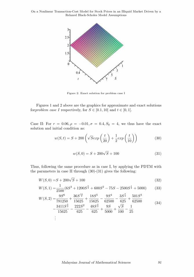
Figure 2: Exact solution for problem case I

Figures 1 and 2 above are the graphics for approximate and exact solutionsforproblem case I respectively, for S ∈ [0.1, 10] and t ∈ [0, 1].

Case II: For r = 0.06, ρ = −0.01, σ = 0.4, S0 = 4, we thus have the exactsolution and initial condition as:

w(S, t) = S + 200

(√Sexp

(t

20

)+

1

2exp

(t

10

))(30)

w(S, 0) = S + 200√S + 100 (31)

Thus, following the same procedure as in case I, by applying the PDTM withthe parameters in case II through (30)-(31) gives the following:

W (S, 0) =S + 200√S + 100 (32)

W (S, 1) =1

2500(6S3 + 1200S

52 + 600S2 − 75S − 2500S

12 + 5000) (33)

W (S, 2) =9S6

781250+

36S112

15625+

18S5

15625− 9S4

62500− 3S

72

625+

501S3

62500

−3411S52

15625− 222S2

625− 48S

32

625+

9S

5000+

√S

100− 1

25

(34)

...



Whence,

w(S, t) =

∞∑h=0

W (S, h)th

=W (S, 0) +W (S, 1)t+W (S, 2)t2 +W (S, 3)t3 + · · ·

=(S + 200√S + 100)

+

(1

2500

(6S3 + 1200S

52 + 600S2 − 75S − 2500S

12 + 5000

))t

+

(9S6

781250+

36S112

15625+

18S5

15625− 9S4

62500− 3S

72

625+

501S3

62500

− 3411S52

15625− 222S2

625− 48S

32

625+

9S

5000+

√S

100− 1

25

)t2 + · · ·

(35)

In tables 1- 3, we present in comparison, the exact and the approximatesolutions for time t = 0, 0.5 and 1 respectively. In addition, figure 3 and figure4 below are the graphics for approximate and exact solutions for problem caseII respectively, for t ∈ [1, 2] and S ∈ [0.1, 5].

Table 1: t=0



Table 2: t=0.5

Table 3: t=1

Figure 3: Exact solution for case II



Figure 4: Approximate solution for case II

5. Concluding Remarks

In this paper, we considered a nonlinear transaction-cost model for stockprices in an illiquid market. This nonlinear model was arrived at when theconstant volatility assumption of the classical linear Black-Scholes option pric-ing model was relaxed through the inclusion of transaction cost. We obtainedapproximate solutions to this nonlinear model using the projected differentialtransform method PDTM as a semi-analytical method. The results are very in-teresting, agree with the associated exact solutions obtained by Esekon (2013)and that of Gonzalez-Gaxiola et al. (2015) using the Adomian decompositionmethod; even though our approximate solutions include only terms up to timepower two. All numerical computations and graphics done in this work wereby Maple 18.

Acknowledgement

The authors are honestly thankful to Covenant University for financial assis-tance and provision of good working environment. They also wish to acknowl-edge the anonymous referee(s) for their constructive and helpful comments.

References

Acharya, V. and Pedersen, L. H. (2005). Asset pricing with liquidity risk.Journal of Financial Economics, 77(2):375–410.

Allahviranloo, T. and Behzadi, S. S. (2013). The use of iterative methods forsolving black-scholes equation. International Journal of Industrial Mathe-matics, 5(1):1–11.

Amihud, Y. and Mendelson, H. (1986). Asset pricing and the bid-ask spread.International Journal of Industrial Mathematics, 17:219–223.

Ankudinova, J. and Ehrhardt, M. (2008). On the numerical solution of nonlin-



ear black-scholes equations. Computers and Mathematics with Applications,56(3):799–812.

Bakstein, D. and Howison, S. (2003). A non-arbitrage liquidity model withobservable parameters for derivatives. Oxford University Preprint, UnitedKingdom. Available at http://eprints.maths.ox.ac.uk/53/.

Barles, G. and Soner, H. M. (1998). Option pricing with transaction costs anda nonlinear black-scholes equation. Finance and Stochastics, 2(4):369–397.

Black, F. and Scholes, M. (1973). The pricing options and corporate liabilities.Journal of Political Economy, 81(3):637–654.

Bohner, M. and Zheng, Y. (2009). On analytical solution of the black-scholesequation. Applied Mathematics Letters, 22(3):309–313.

Boyle, P. and Vorst, T. (1992). Option replication in discrete time with trans-action costs. Journal of Finance, 47(1):271–293.

Cen, Z. and Le, A. (2011). A robust and accurate finite difference method fora generalized black- scholes equation. Journal of Computational and AppliedMathematics, 235(13):3728–3733.

Cetin, U., Jarrow, R. A., and Protter, P. (2004). Liquidity risk and arbi-trage pricing theory. Journal of Computational and Applied Mathematics,8(3):311–341.

Company, R., Navarro, E., Pintos, J. R., and Ponsoda, E. (2008). Numeri-cal solution of linear and nonlinear black-scholes option pricing equations.Computers and Mathematics with Applications, 56(3):813–821.

Edeki, S. O., Ugbebor, O. O., and Owoloko, E. A. (2015). Analytical solu-tions of the black-scholes pricing model for european option valuation via aprojected differential transformation method. Entropy, 17(11):7510–7521.

Edeki, S. O., Ugbebor, O. O., and Owoloko, E. A. (2016a). The modified black-scholes model via constant elasticity of variance for stock options valuation.In AIP Conference proceedings. DOI: 10.1063/1.4940289.

Edeki, S. O., Ugbebor, O. O., and Owoloko, E. A. (2016b). A note on black-scholes pricing model for theoretical values of stock options. In AIP Confer-ence proceedings. DOI:10.1063/1.4940288.

Edeki, S. O., Ugbebor, O. O., and Owoloko, E. A. (2016c). On a modified trans-formation method for exact and approximate solutions of linear schrodingerequations. In AIP Conference proceedings. DOI: 101063/1.4940296.

Esekon, J. E. (2013). Analytic solution of a nonlinear black-scholes equation.International Journal of Pure and Applied Mathematics, 82(4):547–555.

Frey, R. and Patie, P. (2002). Risk Management for Derivatives in IlliquidMarkets: A Simulation Study. Springer, Berlin.

Frey, R. and Stremme, A. (1997). Market volatility and feedback effects fromdynamic hedging. Mathematical finance, 7(4):351–374.



Gonzalez-Gaxiola, O., Ruiz de Chavez, J., and Santiago, J. A. (2015). Anonlinear option pricing model through the adomian decomposition method.International Journal of Applied and Computational Mathematics, 1(2):1–15.

Jang, B. (2010). Solving linear and nonlinear initial value problems by the pro-jected differential transform method. Computer Physics Communications,181(5):848–854.

Jdar, L., Sevilla-Peris, P., Corts, J. C., and Sala, R. (2005). A new directmethod for solving the black-scholes equation. Applied Mathematics Letters,18(1):29–32.

Keskin, Y., Servi, S., and Oturanc, G. (2011). Reduced differential transformmethod for solving klein gordon equations. In Proceedings of the WorldCongress on Engineering. London. DOI: 101063/1.4940296.

Keynes, J. M. (1971). A treatise on money: the pure theory of money. Macmil-lan, London. Edited by Johnson, E. and Moggridge, D.

Liu, H. and Yong, J. (2005). Option pricing with an illiquid underlying assetmarket. Journal of Economic Dynamics and Control, 29(12):2125–2156.

Owoloko, E. A. and Okeke, M. C. (2014). Investigating the imperfection of theb-s model: A case study of an emerging stock market. British Journal ofApplied Science and Technology, 4(29):4191–4200.

Ravi Kanth, A. and Aruna, K. (2012). Comparison of two dimensional dtm andptdm for solving time-dependent emden-fowler type equations. InternationalJournal of Nonlinear Science, 13(2):228–239.

Rodrigo, M. R. and Mamon, R. S. (2006). An alternative approach to solvingthe black-scholes equation with time-varying parameters. Applied Mathemat-ics Letters, 19(4):398–402.


Documents

On a Nonlinear Transaction-Cost Model for Stock Prices in ...einspem.upm.edu.my/journal/fullpaper/vol11/7. odeki.pdf · Edeki,S.O.,Ugbebor,O.O.andOwoloko,E.A. 1. Introduction Inaprofessionalsetting,theterm‘liquidity’describestheleveltowhichan