Forecasting Spot Freight Rates using Vector Error ...einspem.upm.edu.my/journal/fullpaper/vol12no2/6. Che mohd Taib.pdf · Taib,C.M.I.C.andMohtar,Z.I. long term relations between

Malaysian Journal of Mathematical Sciences 12(2): 235–253 (2018)

MALAYSIAN JOURNAL OF MATHEMATICAL SCIENCES

Journal homepage: http://einspem.upm.edu.my/journal

Forecasting Spot Freight Rates using VectorError Correction Model in the Dry Bulk Market

Taib, C. M. I. C. ∗ and Mohtar, Z. I.

School of Informatics and Applied Mathematics, UniversitiMalaysia Terengganu, Malaysia

E-mail: [email protected]∗ Corresponding author

Received: 29 July 2017Accepted: 5 March 2018

ABSTRACT

In this paper, we employ an applied econometric study concerning fore-casting the spot freight rates based on Forward Freight Agreement (FFA)and Time Charter (TC) contracts. This study is important since thevolatility of shipping freight rates is quite high and the future develop-ment of the rates is uncertain which may not easily predicted. Empir-ical analysis contains investigation of the relationship between the spotfreight rates with FFA and TC. We also check for stationarity of thosethree types of data. The calibration of vector error correction model(VECM) is carried out using ordinary least square (OLS) method. Later,the VECM is used in forecasting the spot rates. Results show that theFFA forecasts better the spot compared to TC.

Keywords: Vector Error Correction Model, Dry Bulk Market, SpotFreight Rates, Forward Freight Agreement, Time Charter.

Taib, C. M. I. C. and Mohtar, Z. I.

1. Introduction

Volatility of freight rates contributes risk to the participants in freight mar-ket including the shipowner, charterer, shipping banks and shipping hedgefunds. As recorded in the years 2008 to 2011, the annualized volatility ofshipping freight rates varies between 59% to 79%1. The freight rates, whichrepresent the cost of hiring shipping transportation tend to move randomlyover time with its change of direction is determined by the shipping marketcycle. Such rates increase when there is less supply of ship in the market andthe freight rates diminish when there is an exorbitant supply of ship. In thisstudy, we aim at forecasting the spot freight rates based on the time charterand forward rates in international shipping market.

Shipping plays a major role in the world trade where 75% of the volumeof the world trade in manufactured products and commodities are carried outusing this seaborne transportation (see Alizadeh and Nomikos (2009)). Oneof the popular markets in shipping industry is dry bulk where the market isgenerally categorized either as major bulk (delivery of for instance iron ore, coaland grain) or minor bulk (delivery of for instance agricultural products, steeland mineral cargoes). Based on the vessel size and route, several markets indry bulk are Capesize, Panamax, Supramax and Handysize. Reader may referto Alizadeh et al. (2015) for a detailed explanation of the dry bulk markets.

The risk management techniques applied on commodities and financial mar-kets could also be developed for risk management in the shipping industry.Traditionally, the risk of freight rate is managed by the time charter (TC) con-tract. A TC contract is an agreement between the shipowner and chartererwhere the charterer hire the vessel from the shipowner for a specific period oftime (see Tezuka et al. (2012) and Zhang and Zeng (2015)). Such agreementin terms of duration and freight rates between those participants are recordedby charter party. However, the vessel is still under supervision of the shipownerwhile all the expenses and the direction of the vessel are under responsibilitiesof the charterer.

The Baltic International Freight Futures Exchange (BIFFEX) is the firstexchange-traded freight futures contract and later the Forward Freight Agree-ments (FFA) provide dynamic hedges for participants. By definition, FFA isa contract between two parties to hire or settle the freight rates for a certaintype of cargo at a future date. The development of shipping derivative resultsin an immense growth of the futures markets over the years. However, FFA

1The paper was presented by N. Nomikos at Cass Business School, City University London.See http://www.bbk.ac.uk/cfc/papers/nomikos.pdf for a detailed report.

236 Malaysian Journal of Mathematical Sciences

Forecasting Spot Freight Rates using Vector Error Correction Model in the Dry BulkMarket

market is still under research and considered interesting compared to otherfreight derivatives because the underlying asset in the market is not a storablecommodity but is a service.

The FFA becomes a popular derivative tool in the shipping industry andit allows price discovery and hedging just like other financial derivative (seeKavussanos and Visvikis (2004)). The contract owner has the right to buyor sell the freight rate at a certain date in the future by using the FFA. Fur-thermore, FFA market also high in liquidity as it allows the shipping marketparticipant to enter and exit the market without causing extreme changes inprice (see Alizadeh et al. (2015)). According to Alizadeh (2013), FFA marketgrew rapidly between the years 2003 until 2009 and reached the peak at 2007with 2.3 million trading. In arbitrage dominated markets, the spot rates areclosely tied to the forward rates. The spot rates move in the direction towardsforward to ensure convergence at the expiration date. Thus, the forward ratesare unbiased forecasts of future spot rates (see Kavussanos et al. (2004) andAlnes and Marheim (2013)).

Modelling and forecasting of spot freight rates has been studied by manyresearchers neither it is done theoretically nor empirically. Among them areKavussanos and Alizadeh (2001, 2002), Jonnala et al. (2002), Rygaard (2009)and recently in a paper by Benth et al. (2015). To mention a few, a study doneby Rygaard (2009) used a dynamic programming approach to determine thevalue of a TC contract using vector error correction model (VECM). The studyindicates that the price of ship is correlated for a long time charter contractbut not for a short time contract. Further, six different continuous stochasticmodels of spot freight rates have been introduced in Benth et al. (2015). Theyfind that their proposed dynamical models are fitted to market data and themodels also can be used in risk management studies. However, in this paper,we only focus on forecasting the spot freight rates using VECM.

The general model of vector autoregression (VAR) is a flexible model andcommonly used for multivariate time series analysis. The model is very helpfulin forecasting and interpreting the dynamic performance of financial and eco-nomic time series. In order to use the model, all variables must be stationarywith a similar order of integration.

However, in the case of non-stationary and exists co-integration betweenthe variables, then error correction term will be added into VAR model. Suchmodel is referred as VECM and also known as a restricted VAR. VECM is aneconometric model that has been frequently used for modelling and forecastingspot freight rates, and also proven to be efficient in estimating the short and

Malaysian Journal of Mathematical Sciences 237


long term relations between variables. Examples of papers discovering thisissue are Veenstra and Franses (1997), Batchelor et al. (2007), Spreckelsenet al. (2012) and Zhang et al. (2014).

The literature also has demonstrated the use of various econometric modelsin predicting the spot prices. For instance, Cullinane (1992) and Cullinaneet al. (1999) reported the success of forecasting the spot freight rates usingsimpler univariate autoregressive integrated moving average (ARIMA) models.Zeng and Swanson (1998) estimate five models including VECM for spot andfutures prices of the US 30-year Treasury bond, oil, gold and the S&P500index. They find that the VECM produces more accurate forecasts than allsimpler models in a shorter horizon. Furthermore, Kavussanos and Nomikos(2003) compared the forecasting performance of VAR, VECM, random walkand ARIMA models. They also find that VECM predicts better of spot pricescompared to the other models but not of futures prices as reported in the paperby Batchelor et al. (2007). As the forecast horizons increases, the predictingability of VECM is getting better. However, VECM can only be used if aco-integration relationship exist between the variables. Thus, the relationshipbetween variables shall be initially determined in order to use the VECM modelfor forecasting.

The rest of the paper is organised as follows: Section 2 briefly discussesforecasting model and the relevant tests. In Section 3 we analyse the empiricalspot freight rates and calibrating the model. Next, we derive the forecastingperformance in Section 4 and finally conclusion ends the paper.

2. Forecasting model of the spot freight rates

In this section, we explain the VECM model together with appropriate testsused for the purpose of forecasting the spot freight rates. The parameters ofVECM based on FFA and TC are calibrated and finally we forecast the spotfreight rates using such model.

2.1 Correlation analysis

Correlation analysis measures the strength between two variables whetherthey move in same direction or opposite direction. Correlation coefficient isvalued between −1 to 1 as shown in Table 1. The coefficient −1 indicates thatthe markets are moving in opposite direction, 0 indicates no direction betweenthe markets and 1 indicates the markets are moving together in same direction.



Table 1: Correlation analysis.

Correlation coefficient Strength of correlation-1 Strongly negative0 No correlation1 Strongly positive

2.2 Augmented Dickey-Fuller test

Raw data are often in non-stationary form and can have specific cycle,trend, seasonality or random walk. This means that variance, covariance andmean of the data are changing over the time which will affect the reliabilityand consistency of the time series result (see Franses and McAleer (1998)).In order to have a consistent result, Augmented Dickey-Fuller (ADF) test isused to check the stationarity of the data. The series of data will be testedif it needs to be differenced in order to make it stationary. The following testequation is used:

∆zt = α0 + θzt−1 + γt+ α1∆zt−1 + α2∆zt−2 + · · ·+ αp∆zt−p + et, (1)

where zt is time series, ∆ is difference operator, αi is parameter, γ is coefficienton a time trend, t is time index, p is lag order of the first-differences autoregres-sive process and et is independent identically distributes residual term. Theequation has an intercept term and a time trend. Hence, it is only suitable fora data series with a trend.

The null hypothesis of the ADF t-test is

H0 : θ = 0, (unit root test is present)

against the following alternative hypothesis

H1 : θ < 0; (unit root test is absent).

If the null hypothesis is accepted, the data need to be differenced to makeit stationary and the Johansen Co-Integration test can be later carried out. Onthe contrary, the rejection of null hypothesis means that the data is stationaryand can be analysed by using a time trend in the regression model instead ofdifferencing.



2.3 Johansen co-integration test

Johansen test allows more than one co-integrating relationship. This test isbetter than Eagle-Granger test which allows only one co-integration relation.When there are more than two variables, all co-integrating vectors can beestimated since the Johansen test is a likelihood-ratio test (see Mallory andLence (2012)). Generally, there are at most n−1 co-integrating vectors if thereare n variables which all have unit roots. The long term relationship amongthe data set can be determined by using Johansen test.

There are two types of Johansen test: the trace and maximum eigenvaluetests. For the trace test, it is used to test if the rank of the matrix, Π is r0. Rank(Π) = r0 is the null hypothesis. The alternative hypothesis is r0 < rank(Π) ≤ n,where n is the maximum number of possible co-integrating vectors. The testequation is as below:

LR(r0, n) = −Tn∑

i=r0+1

ln(1− λi), (2)

where LR(r0, n) is the likelihood-ratio test statistic for testing whether rank(Π) = r0 versus the alternative hypothesis that rank (Π) ≤ n. For the succeed-ing test if this null hypothesis is rejected, the next null hypothesis is that rank(Π) = r0 + 1 and the alternative hypothesis is that r0 + 1 < rank(Π) ≤ n.

Next, the maximum eigenvalue test is used to determine whether the largesteigenvalue is zero relative to the alternative that the next largest eigenvalue iszero. The first test is a test whether the rank of the matrix Π is zero. The nullhypothesis is that rank (Π) = 0 and the alternative hypothesis is that rank(Π) = 1. For further tests, the null hypothesis is that rank (Π) = 1, 2, . . . andthe alternative hypothesis is that rank (Π) = 2, 3, . . . ,

The test equation is as below:

LR(r0, r0 + 1) = −T ln(1− λr0+1), (3)

where LR(r0, r0 + 1) is the likelihood-ratio test statistic for testing whetherrank (Π) = r0 versus the alternative hypothesis that rank (Π) = r0 + 1.



2.4 Vector error correction model

If the data series are co-integrated and long run relationship exists betweenthe variables, then this model can be used for forecasting. Let St, Wt and Ft

represent the spot rates, TC rates and FFA prices respectively. The VECM(p) for spot rates and TC rates is written as follows:

∆St =

p−1∑i=1

aS,i∆St−i +

p−1∑i=1

bS,i∆Wt−i + αSzt−1 + εS,t; (4)

∆Wt =

p−1∑i=1

aW,i∆St−i +

p−1∑i=1

bW,i∆Wt−i + αW zt−1 + εW,t, (5)

where ∆ denotes the first difference operator, aS,i, aW,i, bS,i, bW,i are coeffi-cients, εS,t and εW,t are error terms, αS and αW are error correction coefficientsand zt−1 is the error correction term.

The VECM (q) for spot rates and FFA prices is written as follows:

∆St =

q−1∑i=1

aS,i∆St−i +

q−1∑i=1

cS,i∆Ft−i + αSzt−1 + εS,t; (6)

∆Ft =

q−1∑i=1

aF,i∆St−i +

q−1∑i=1

cF,i∆Ft−i + αF zt−1 + εF,t, (7)

where ∆ denotes the first difference operator, aS,i, aF,i, cS,i, cF,i are coefficients,εS,t and εF,t are error terms, αS and αF are error correction coefficients andzt−1 is the error correction term.

2.5 Calibration of parameters

The calibration of parameters is carried out by using the Ordinary LeastSquare (OLS) method. In statistical analysis, this method is the simplest typeof estimation technique and is used to fit a function closely with the data byminimizing the sum of squared errors from the data. The R-squared value,R2 is also determined with the value ranging from 0 to 1 where 0 indicates no



improvement in the forecasting and 1 indicates the forecasting model predictsperfectly. The equation is as shown below:

yi =

k∑j=0

BjXij + εi, (8)

where y is dependent variable, B is coefficient, X is independent variable andε is error term.

2.6 Forecasting accuracy

The measures of mean absolute deviation (MAD) and root mean squarederror (RMSE) are selected to compare the forecasting accuracy since both ap-proaches are really good accuracy measures (see Batchelor et al. (2007)). Ac-cording to Meese and Rogoff (1983), the MAD is more appropriate and reliablebecause it less sensitive to the presence of outliers while a study done by Er-icsson (1992) shows that "forecast encompassing" proposed by Chong andHendry (1986) is the sufficient condition of the RMSE dominance (see Ashiya(2007) and Kuo (2016)). The smaller the values of MAD and RMSE, the bet-ter the predicting ability of the model. The MAD and RMSE are respectivelygiven by

MAD =

∑Ni=1 |yi − yi|

N(9)

and

RMSE =

√∑Ni=1(yi − yi)2

N, (10)

where N is the number of forecast, yi are predicted values and yi are real values.



3. Empirical analysis of the freight rates

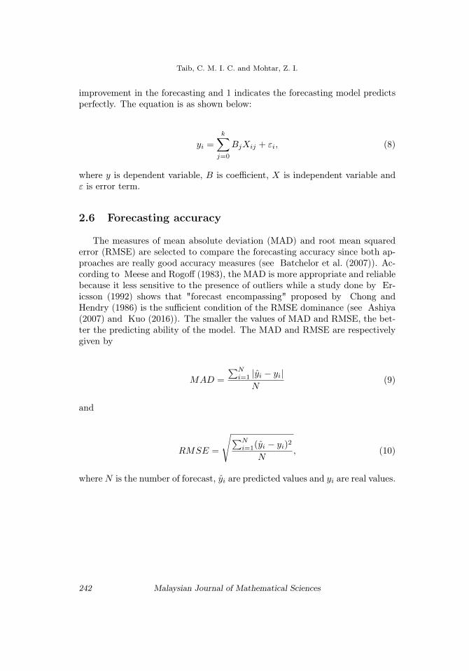
The data of spot freight rates and time charter for the segment of BalticCapesize Index (BCI) are obtained from Baltic Exchange2 while the FFA pricesare obtained from Baltic Forward Assessments (BFA). The chosen series of spotrate is the BCI 4T/C which is the four time charter routes average and the TCrates consist of the prices of TC contracts for 6-month. The TC contract is fordry bulk vessels of 170,000 metric tons (Mt) dead weight tonnage (Dwt). Thedata set of spot rates, 6-month TC prices and FFA prices for Capesize marketare observed from January 6, 2006 until June 5, 2009. The TC and FFA dataare arranged to synchronize with the spot data.

Figure 1: Time series of Spot, FFA and TC prices

Figure 1 shows that the spot prices closely follow with FFA and TC pricesand there is a high consistency between the three prices. Result of correlationcoefficient in Table 2 indicates the high correlation between spot, FFA and TC.

Table 2: Correlation Coefficient between Spot, FFA and TC prices.

FFA Spot TCFFA 1.000000 0.959908 0.982610Spot 0.959908 1.000000 0.974596TC 0.982610 0.974596 1.000000

2See http://www.balticexchange.com for detailed information of daily quotes for differentroutes and indices in various shipping segments.



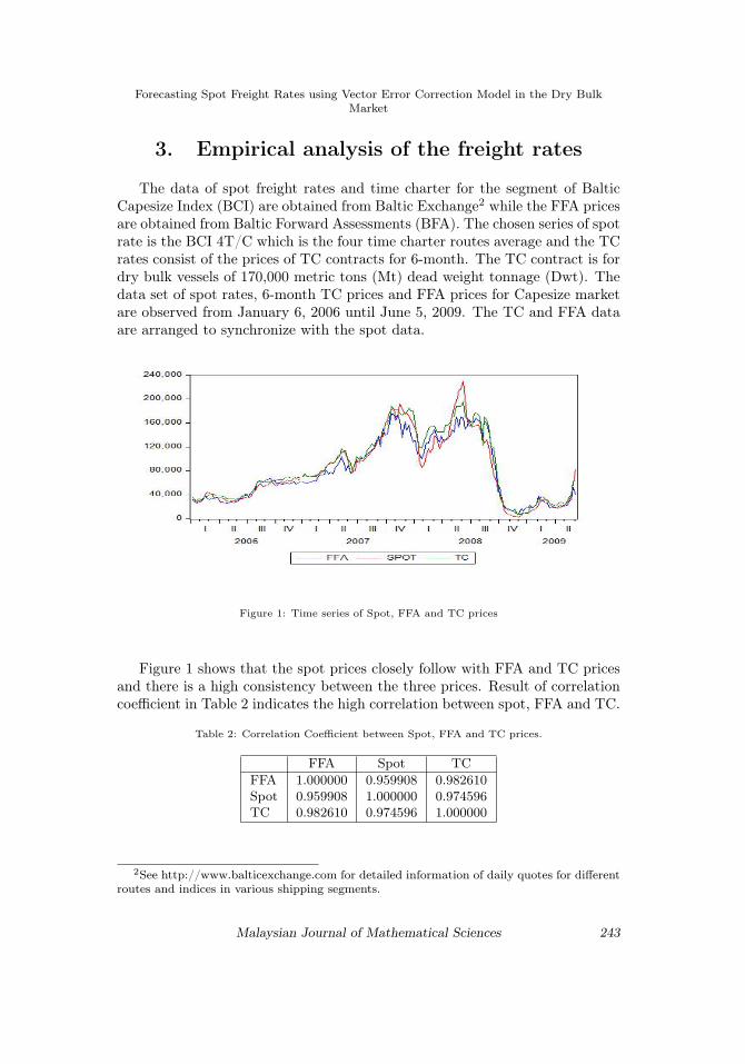
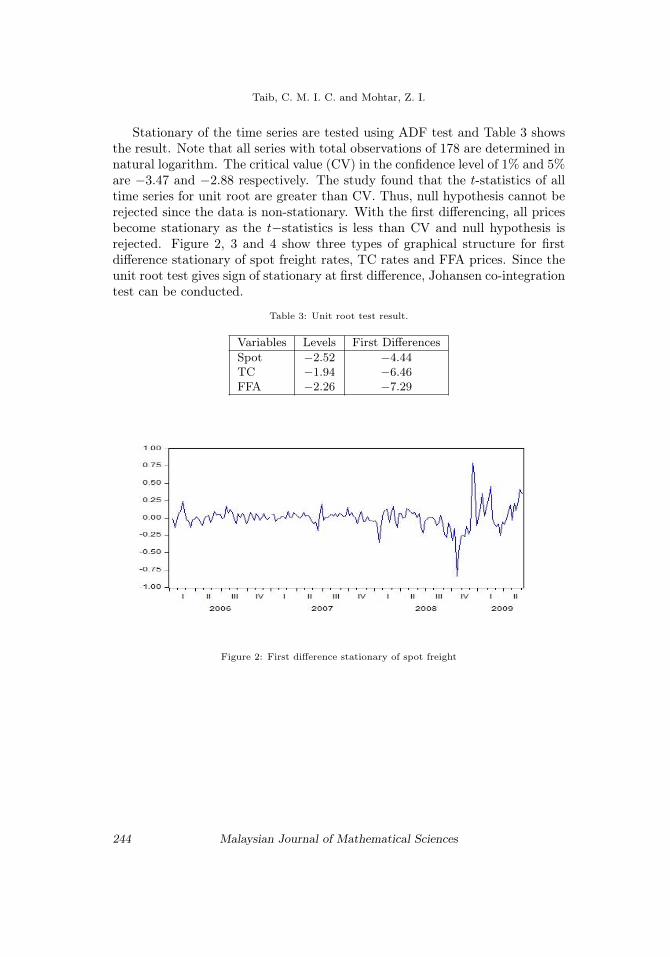
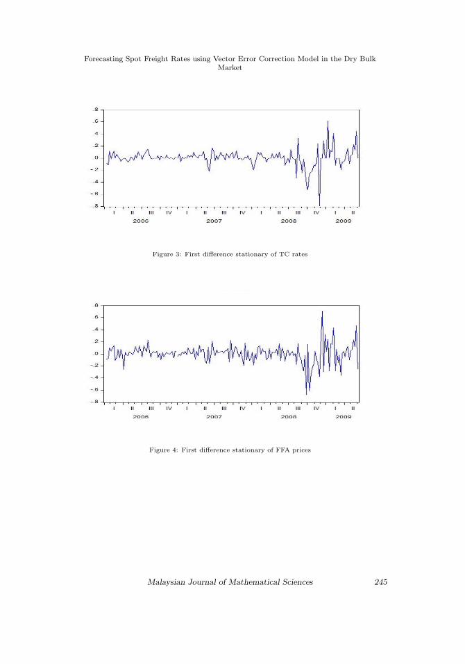
Stationary of the time series are tested using ADF test and Table 3 showsthe result. Note that all series with total observations of 178 are determined innatural logarithm. The critical value (CV) in the confidence level of 1% and 5%are −3.47 and −2.88 respectively. The study found that the t-statistics of alltime series for unit root are greater than CV. Thus, null hypothesis cannot berejected since the data is non-stationary. With the first differencing, all pricesbecome stationary as the t−statistics is less than CV and null hypothesis isrejected. Figure 2, 3 and 4 show three types of graphical structure for firstdifference stationary of spot freight rates, TC rates and FFA prices. Since theunit root test gives sign of stationary at first difference, Johansen co-integrationtest can be conducted.

Table 3: Unit root test result.

Variables Levels First DifferencesSpot −2.52 −4.44TC −1.94 −6.46FFA −2.26 −7.29

Figure 2: First difference stationary of spot freight



Figure 3: First difference stationary of TC rates

Figure 4: First difference stationary of FFA prices



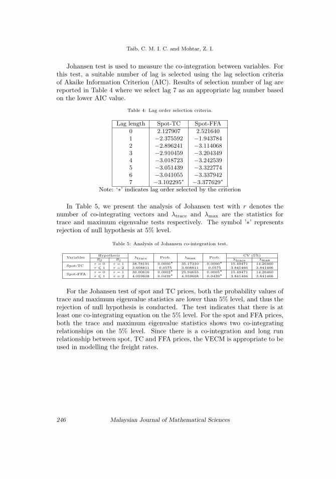
Johansen test is used to measure the co-integration between variables. Forthis test, a suitable number of lag is selected using the lag selection criteriaof Akaike Information Criterion (AIC). Results of selection number of lag arereported in Table 4 where we select lag 7 as an appropriate lag number basedon the lower AIC value.

Table 4: Lag order selection criteria.

Lag length Spot-TC Spot-FFA0 2.127907 2.5216401 −2.375592 −1.9437842 −2.896241 −3.1140683 −2.910459 −3.2043494 −3.018723 −3.2425395 −3.051439 −3.3227746 −3.041055 −3.3379427 −3.102295∗ −3.377629∗

Note: ‘∗’ indicates lag order selected by the criterion

In Table 5, we present the analysis of Johansen test with r denotes thenumber of co-integrating vectors and λtrace and λmax are the statistics fortrace and maximum eigenvalue tests respectively. The symbol ’∗’ representsrejection of null hypothesis at 5% level.

Table 5: Analysis of Johansen co-integration test.

Variables Hypothesisλtrace Prob. λmax Prob. CV (5%)

H0 H1 λtrace λmax

Spot-TC r = 0 r = 1 38.78191 0.0000∗ 35.17310 0.0000∗ 15.49471 14.26460r 6 1 r = 2 3.608811 0.0575 3.608811 0.0575 3.841466 3.841466

Spot-FFA r = 0 r = 1 30.00616 0.0002∗ 25.94655 0.0005∗ 15.49471 14.26460r 6 1 r = 2 4.059608 0.0439∗ 4.059608 0.0439∗ 3.841466 3.841466

For the Johansen test of spot and TC prices, both the probability values oftrace and maximum eigenvalue statistics are lower than 5% level, and thus therejection of null hypothesis is conducted. The test indicates that there is atleast one co-integrating equation on the 5% level. For the spot and FFA prices,both the trace and maximum eigenvalue statistics shows two co-integratingrelationships on the 5% level. Since there is a co-integration and long runrelationship between spot, TC and FFA prices, the VECM is appropriate to beused in modelling the freight rates.



Table 6: Analysis of spot and TC prices on the sample (weekly).

Parameters Coefficients ∆St Coefficients ∆Wt

∆St−1 aS,10.521907

aW,10.253707

(5.79301∗) (2.61340∗)

∆St−2 aS,2−0.082637

aW,2−0.100033

(−0.84048) (−0.94419)

∆St−3 aS,30.157979

aW,30.280342

(1.64525) (2.70947∗)

∆St−4 aS,40.025309

aW,4−0.015594

(0.26497) (−0.15151)

∆St−5 aS,5−0.000536

aW,5−0.021080

(−0.00564) (−0.20584)

∆St−6 aS,60.116164

aW,60.232553

(1.31963) (2.45170∗)

∆St−7 aS,7−0.229518

aW,7−0.018945

(−2.83247∗) (−0.21698)

∆Wt−1 bS,10.329893

bW,10.034257

(3.27953∗) (0.31604)

∆Wt−2 bS,2−0.236415

bW,20.061115

(−2.55247∗) (0.61234)

∆Wt−3 bS,30.097586

bW,3−0.025085

(1.02070) (−0.24349)

∆Wt−4 bS,40.288770

bW,40.055313

(3.06530∗) (0.54489)

∆Wt−5 bS,5−0.004084

bW,5−0.090711

(−0.04637) (−0.95574)

∆Wt−6 bS,60.066968

bW,6−0.338671

(0.76507) (−3.59070∗)

∆Wt−7 bS,70.160584

bW,7−0.121907

(1.77063) (−1.24743)

Zt−1 αS−0.269007

αW0.122073

(−3.48995∗) (1.46974)

R2 0.570850 0.314104

The calibration of VECM model is carried out using the OLS method forestimation period from January 6, 2006 to June 5, 2009. The results are pre-sented in Table 6 and 7. Note that the values in bracket are t−statistics andthe symbol ‘∗’ is the significance indicator at 5% level.

Based on Table 6, the estimated coefficients of aS,1, aW,1, aW,3, aW,6, aS,7,bS,1, bS,2, bS,4, bW,6, αS are statistically significant. Furthermore, it has beenproven that a bidirectional lead-lag relationship exists between spot and TCprices if the coefficients are significant (see Kavussanos and Visvikis (2004)).In Table 7, we report the estimated coefficients for spot and FFA prices. Similarto spot rates and TC prices, the estimated coefficients of aS,1, aS,2, aF,3, aS,4,aF,4, aS,7, cS,1, cF,2, cS,4, cS,5, cF,5, αS are statistically significant. Thus, abidirectional causal relationship exists between spot and FFA prices. Besides,a moderate R2 indicates that our model fits the data well.



Table 7: Analysis of spot and FFA prices on the sample (weekly).

Parameters Coefficients ∆St Coefficients ∆Ft

∆St−1 aS,10.284039

aF,1−0.158310

(2.84128∗) (−1.06642)

∆St−2 aS,2−0.235972

aF,20.037889

(−2.21062∗) (0.23903)

∆St−3 aS,30.117766

aF,30.397666

(1.07701) (2.44908∗)

∆St−4 aS,4−0.298388

aF,4−0.624203

(−2.69989∗) (−3.80344∗)

∆St−5 aS,50.113721

aF,50.192906

(1.00295) (1.14570)

∆St−6 aS,6−0.065084

aF,6−0.003015

(−0.59459) (−0.01855)

∆St−7 aS,7−0.138983

aF,7−0.072325

(−2.17281∗) (−0.76143)

∆Ft−1 cS,10.577922

cF,1−0.054652

(7.94004∗) (−0.50565)

∆Ft−2 cS,20.072870

cF,20.410398

(0.77860) (2.95293∗)

∆Ft−3 cS,30.129292

cF,3−0.072048

(1.33942) (−0.50264)

∆Ft−4 cS,40.209184

cF,40.138963

(2.17396∗) (0.97254)

∆Ft−5 cS,50.389728

cF,50.403082

(4.09783∗) (2.85412∗)

∆Ft−6 cS,60.076877

cF,6−0.047204

(0.79335) (−0.32804)

∆Ft−7 cS,70.166821

cF,70.137312

(1.77407) (0.98337)

Zt−1 αS−0.087890

αF−0.060518

(−3.68285∗) (−1.70772)

R2 0.684413 0.239646

4. Forecasting performance

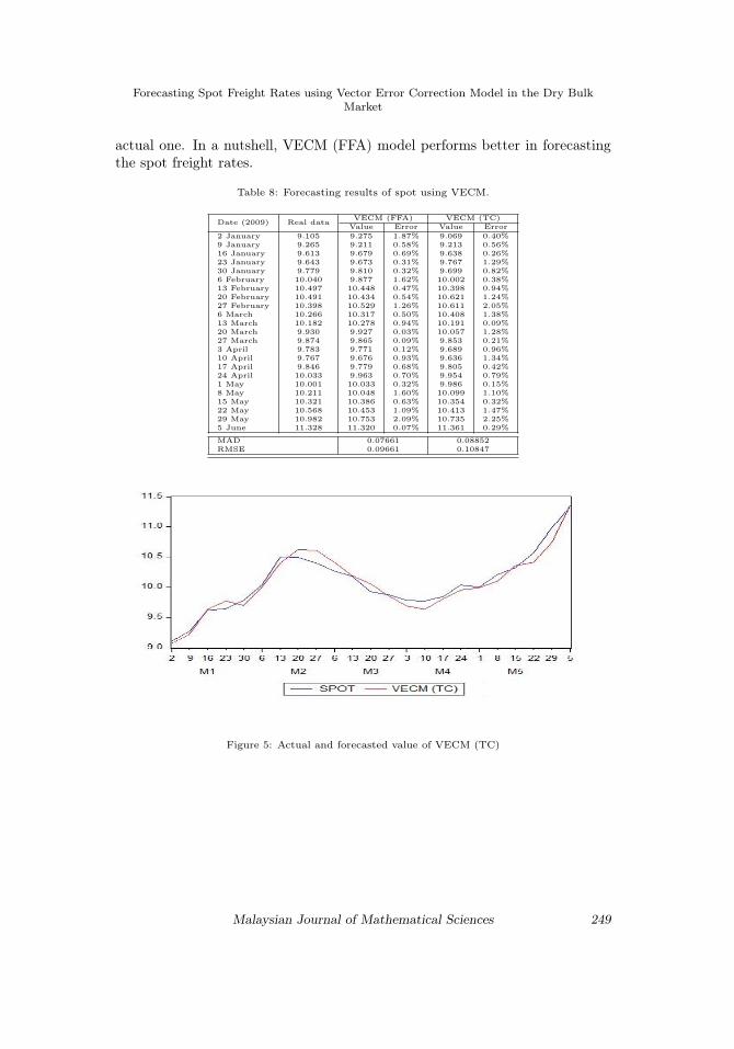
We use parameters of VECM model obtained in previous section to forecastthe spot freight rates. The forecasting sample is from January 2, 2009 untilJune, 5 2009 with 23 numbers of observation. One step ahead forecast is usedand Table 8 shows the result. The forecast error is the difference betweenforecasted and actual values. The forecasted value of spot rates is comparedwith the actual value of spot rates to determine the percentage of error. Thefirst column in Table 8 is the real spot rates for BCI 4T/C and the secondcolumn is the results for the spot rates forecasting model based on spot and FFArates (VECM (FFA)). The last column is the results for spot rates forecastingmodel based on spot and TC rates (VECM (TC)). Note that the data seriesfor real and forecasting are measured in natural logarithm.

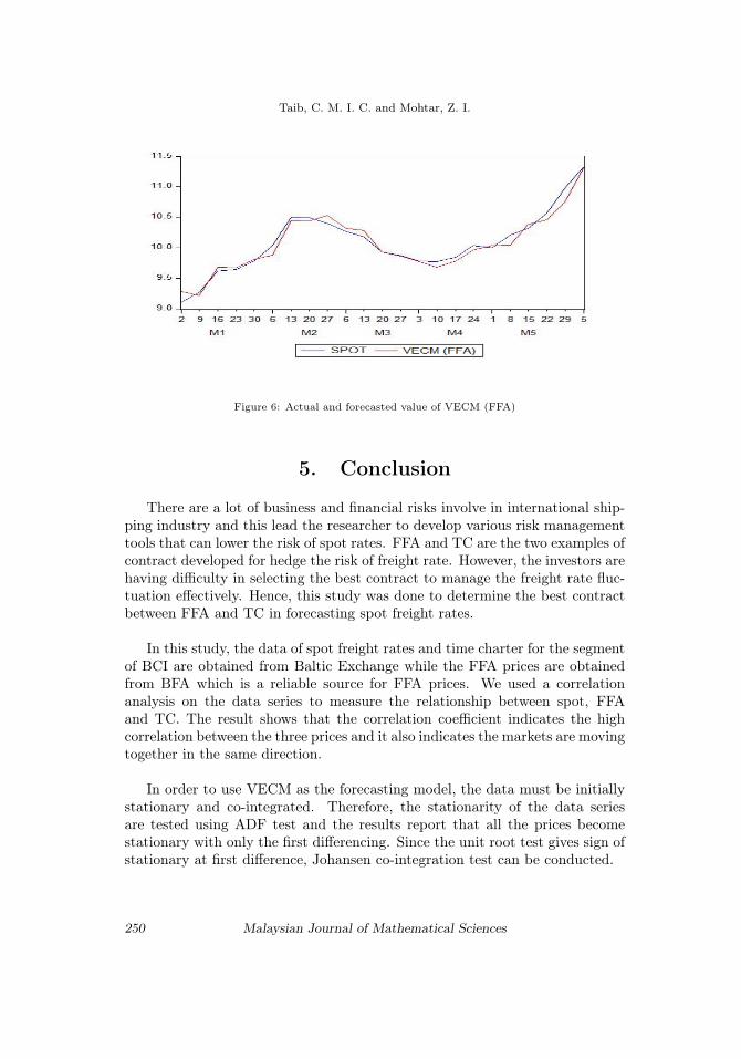
To analyse forecasting performance, two forecast errors, MAD and RMSEare being used. The calculated MAD for VECM (FFA) is less than MAD forVECM (TC) which reveal that VECM (FFA) predict better. Furthermore, theRMSE for VECM (TC) is higher than RMSE for VECM (FFA) which provesthat FFA prices forecast the more accurate spot rates. The forecasted resultsof both FFA and TC are represented in Figures 5 and 6. It is clear that theforecasted spot rates based on TC contract deviate far from the actual spotrates compared to forecasted spot rate using FFA which appear closer to the



actual one. In a nutshell, VECM (FFA) model performs better in forecastingthe spot freight rates.

Table 8: Forecasting results of spot using VECM.

Date (2009) Real data VECM (FFA) VECM (TC)Value Error Value Error

2 January 9.105 9.275 1.87% 9.069 0.40%9 January 9.265 9.211 0.58% 9.213 0.56%16 January 9.613 9.679 0.69% 9.638 0.26%23 January 9.643 9.673 0.31% 9.767 1.29%30 January 9.779 9.810 0.32% 9.699 0.82%6 February 10.040 9.877 1.62% 10.002 0.38%13 February 10.497 10.448 0.47% 10.398 0.94%20 February 10.491 10.434 0.54% 10.621 1.24%27 February 10.398 10.529 1.26% 10.611 2.05%6 March 10.266 10.317 0.50% 10.408 1.38%13 March 10.182 10.278 0.94% 10.191 0.09%20 March 9.930 9.927 0.03% 10.057 1.28%27 March 9.874 9.865 0.09% 9.853 0.21%3 April 9.783 9.771 0.12% 9.689 0.96%10 April 9.767 9.676 0.93% 9.636 1.34%17 April 9.846 9.779 0.68% 9.805 0.42%24 April 10.033 9.963 0.70% 9.954 0.79%1 May 10.001 10.033 0.32% 9.986 0.15%8 May 10.211 10.048 1.60% 10.099 1.10%15 May 10.321 10.386 0.63% 10.354 0.32%22 May 10.568 10.453 1.09% 10.413 1.47%29 May 10.982 10.753 2.09% 10.735 2.25%5 June 11.328 11.320 0.07% 11.361 0.29%

MAD 0.07661 0.08852RMSE 0.09661 0.10847

Figure 5: Actual and forecasted value of VECM (TC)



Figure 6: Actual and forecasted value of VECM (FFA)

5. Conclusion

There are a lot of business and financial risks involve in international ship-ping industry and this lead the researcher to develop various risk managementtools that can lower the risk of spot rates. FFA and TC are the two examples ofcontract developed for hedge the risk of freight rate. However, the investors arehaving difficulty in selecting the best contract to manage the freight rate fluc-tuation effectively. Hence, this study was done to determine the best contractbetween FFA and TC in forecasting spot freight rates.

In this study, the data of spot freight rates and time charter for the segmentof BCI are obtained from Baltic Exchange while the FFA prices are obtainedfrom BFA which is a reliable source for FFA prices. We used a correlationanalysis on the data series to measure the relationship between spot, FFAand TC. The result shows that the correlation coefficient indicates the highcorrelation between the three prices and it also indicates the markets are movingtogether in the same direction.

In order to use VECM as the forecasting model, the data must be initiallystationary and co-integrated. Therefore, the stationarity of the data seriesare tested using ADF test and the results report that all the prices becomestationary with only the first differencing. Since the unit root test gives sign ofstationary at first difference, Johansen co-integration test can be conducted.



Johansen test is used to measure the co-integration between variables. Thetrace and maximum eigenvalue test for the Johansen test of spot and TC pricesindicate the existence of one co-integrating equation on the 5% level. Mean-while, for the spot and FFA prices, both the trace and maximum eigenvaluetest shows two co-integrating relationships on the 5% level. The VECM is ap-propriate to be used in modelling the freight rates since there is a co-integrationand long run relationship between spot, TC and FFA prices.

The calibration of VECM model is carried out using the OLS method.The results show that some estimated coefficients of spot and TC prices aresignificant. Similarly, some estimated coefficients of spot and FFA prices arereported statistically significant. These indicates that a bidirectional lead-lagrelationship exists between the variables. Besides, for the spot rate forecastingmodel based on spot and FFA prices, the R2 shows a higher value comparedto the R2 of spot and TC prices.

Finally, to forecast the spot freight rates we use parameters of VECM modelobtained previously. One step ahead forecast is used as a measurement method,namely static forecast. To determine the percentage of error, the forecastedvalue of spot rates is compared with the actual value of spot rates. Further,two forecast error, MAD and RMSE are being used to analyse the forecastingperformance. The calculated MAD and RMSE for VECM (FFA) are less thanVECM (TC) which reveal that VECM (FFA) predict better. Hence, the FFAcontract is the best and the most suitable method to manage the volatility ofthe freight market.

Acknowledgement

The authors acknowledges financial support from Malaysian Ministry ofHigher Education under grant FRGS:59832.

References

Alizadeh, A. H. (2013). Trading volume and volatility in the shipping forwardfreight market. Transportation Research Part E, 49:250–265.

Alizadeh, A. H., Kappou, K., Tsouknidis, D., and Visvikis, I. (2015). Liquid-ity effects and ffa returns in the international shipping derivatives market.Transportation Research Part E, 76:58–75.



Alizadeh, A. H. and Nomikos, N. (2009). Shipping derivatives and risk man-agement. Palgrave.

Alnes, P. A. and Marheim, M. (2013). Can shipping freight rate risk be reducedusing forward freight agreements? Master’s thesis, Norwegian University ofLife Sciences, AS, Norway.

Ashiya, M. (2007). Forecast accuracy of the japanese government: Its year-ahead gdp forecast is too optimistic. Japan and the World Economy, 19:68–85.

Batchelor, R., Alizadeh, A. H., and Visvikis, I. D. (2007). Forecasting spot andforward prices in the international freight market. International Journal ofForecasting, 23:101–114.

Benth, F. E., Koekebakker, S., and Taib, C. (2015). Stochastic dynamicalmodelling of spot freight rates. IMA Journal of Management Mathematics,26:273–297.

Chong, Y. Y. and Hendry, D. F. (1986). Econometric evaluation of linearmacro-economic models. Review of Economic Studies, 53:671–690.

Cullinane, K. P. B. (1992). A short-term adaptive forecasting model for biffexspeculation: A box-jenkins approach. Maritime Policy and Management,19:91–114.

Cullinane, K. P. B., Mason, K. J., and Cape, M. B. (1999). A comparison ofmodels for forecasting the baltic freight index: Box-jenkins revisited. Inter-national Journal of Maritime Economics, 1:15–39.

Ericsson, N. R. (1992). Parameter constancy, mean square forecast errors, andmeasuring forecast performance: An exposition, extensions, and illustration.Journal of Policy Modeling, 14:465–495.

Franses, P. H. and McAleer, M. (1998). Testing for unit roots and non-lineartransformations. Journal of Time Series Analysis, 19:147–164.

Jonnala, S., Fuller, S., and Bessler, D. (2002). A garch approach to modellingocean grain freight rates. International Journal of Maritime Economics,4:103–125.

Kavussanos, M. G. and Alizadeh, A. H. (2001). Seasonality patterns in drybulk shipping spot and time charter freight rates. Transportation ResearchPart E, 37:443–467.

Kavussanos, M. G. and Alizadeh, A. H. (2002). The expectations hypothesisof the term structure and risk premium in dry bulk shipping freight markets.Journal of Transport Economics and Policy, 36:267–304.



Kavussanos, M. G. and Nomikos, N. K. (2003). Price discovery, causality andforecasting in the freight futures market. Review of Derivatives Research,6:203–230.

Kavussanos, M. G. and Visvikis, I. D. (2004). Market interactions in returnsand volatilities between spot and forward shipping freight markets. Journalof Banking & Finance, 28:2015–2049.

Kavussanos, M. G., Visvikis, I. D., and Menachof, D. (2004). The unbiasednesshypothesis in the freight forward market: Evidence from co-integration tests.Review of Derivatives Research, 7:241–266.

Kuo, C. Y. (2016). Does the vector error correction model perform better thanothers in forecasting stock price? an application of residual income valuationtheory. Economic Modelling, 52:772–789.

Mallory, M. and Lence, S. H. (2012). Testing for co-integration in the presenceof moving average errors. Journal of Time Series Econometrics, 4:1–68.

Meese, R. A. and Rogoff, K. (1983). Empirical exchange rate models of theseventies: Do they fit out of sample? Journal of International Economics,14:3–24.

Rygaard, J. M. (2009). Valuation of time charter contracts for ships. MaritimePolicy and Management, 36:525–544.

Spreckelsen, C., Mettenheim, H. J., and Breitner, M. H. (2012). Spot andfreight rate futures in the tanker shipping market: Short-term forecastingwith linear and non-linear methods. In Helber, S. e. a., editor, OperationsResearch Proceedings 2012, pages 247–252. Springer International PublishingSwitzerland.

Tezuka, K., Ishii, M., and Ishizaka, M. (2012). An equilibrium price model ofspot and forward shipping freight markets. Transportation Research Part E,48:730–742.

Veenstra, A. and Franses, P. (1997). A co-integration approach to forecastingfreight rates in the dry bulk shipping sector. Transportation Research PartA, 31:447–458.

Zeng, T. and Swanson, N. R. (1998). Predictive evaluation of econometricforecasting models in commodity futures markets. Studies in Nonlinear Dy-namics and Econometrics, 2:1037.

Zhang, H. and Zeng, Q. (2015). A study of the relationship between timecharter and spot freight rates. Applied Economics, 47:955–965.



Zhang, J., Zeng, Q., and Zhao, X. (2014). Forecasting spot freight rates basedon forward freight agreement and time charter contract. Applied Economics,46:3639–3648.


Documents

Forecasting Spot Freight Rates using Vector Error ...einspem.upm.edu.my/journal/fullpaper/vol12no2/6. Che mohd Taib.pdf · Taib,C.M.I.C.andMohtar,Z.I. long term relations between