On a coeﬃcient concerning an ill-posed Cauchy problem and ... · Cauchy problem and the singularity detection with the wavelet transform Naohiro Fukuda and Tamotu Kinoshita Abstract

Rend. Istit. Mat. Univ. TriesteVolume 45 (2013), 97–121

On a coefficient concerning an ill-posed

Cauchy problem and the singularity

detection with the wavelet transform

Naohiro Fukuda and Tamotu Kinoshita

Abstract. We study the Cauchy problem for 2nd order weakly hyper-bolic equations. F. Colombini, E. Jannelli and S. Spagnolo showed acoefficient giving a blow-up solution in Gevrey classes. In this paper, weget a simple representation of the coefficient degenerating at an infinitenumber of points, with which the Cauchy problem is ill-posed in Gevreyclasses. Moreover, we also report numerical results of the singularitydetection with wavelet transform for coefficient functions.

Keywords: weakly hyperbolic equations; ill-posed Cauchy problem; Gevrey classes;wavelet transformMS Classification 2010: 35L15; 65J20; 65T60

1. Introduction

We are concerned with the Cauchy problem on [0, T ]×Rx{∂2t u− a(t)∂2

xu = 0,u(0, x) = u0(x), ∂tu(0, x) = u1(x).

(1)

Throughout this paper, we assume the weakly hyperbolic condition, i.e.,

a(t) ≥ 0 for t ∈ [0, T ].

We denote by Gs(R) the space of Gevrey functions satisfying

supx∈K

|∂nx g(x)| ≤ CKrnKn!s for any compact set K ⊂ R, n ∈ N.

From the finite propagation property of hyperbolic equations, it is sufficient toconsider compactly supported initial data u0, u1 and solution u (see [3], [6],[7], etc). Thanks to this fact, we may use the following Gevrey norm for thefunctions on the whole interval R:

‖g‖s,r = supn∈N

‖∂nx g‖L∞(R)

rnn!s.

98 N. FUKUDA AND T. KINOSHITA

We say that the Cauchy problem (1) is well-posed in Gs, if for any u0, u1 ∈ Gs,there is a unique solution u ∈ C2([0, T ];Gs) satisfying the energy estimate:

‖u(t)‖s,R + ‖∂tu(t)‖s,R ≤ CT

(‖u0‖s,r + ‖u1‖s,r

)for t ∈ [0, T ], (2)

where R is a constant greater than r, which implies that the derivative losspossibly occurs in a sense of the radius of the Gevrey class Gs. To know that thederivative loss really occurs, we have a great interest for the counterexample.

There are many kinds of results on the well-posedness for 2nd order weaklyhyperbolic equations (see [2], [4], [5], [6], [9] etc). Let us denote by Ck,α[0, T ](k ∈ N, 0 ≤ α ≤ 1 ) the space of functions having k-derivatives continuous,and the k-th derivative Holder continuous with exponent α on [0, T ]. Especiallyfor the coefficient a ∈ Ck,α[0, T ], F. Colombini, E. Jannelli and S. Spagnolo [4]proved the well-posedness in Gs for 1 < s < 1+(k+α)/2. Moreover, they alsoshowed an example of a coefficient a(t) giving a blow-up solution u as follows:

Theorem 1.1. ([4]) For every T > 0, k ∈ N and 0 ≤ α ≤ 1, it is possible toconstruct a function a(t), C∞ and strictly positive on [0, T ), zero at t = T ,and solution u of (1) in a way that a(t) belongs to Ck,α[0, T ] and u belongs toC1([0, T ), Gs) for s > 1 + (k+ α)/2, whereas {u(t, ·)} is not bounded in D′, ast ↑ T .

Remark 1.2. a ∈ Ck,α[0, T ] means that the zero extension of a(t) belongs toCk,α[0,∞).

Their prior work [5] showed an example of a ∈ C∞[0, T ] giving a blow-up solution u ∈ C1([0, T ), C∞). The main task of the proof of Theorem 1.1is to construct the coefficient a(t) defined piecewise on an infinite number ofintervals between [0, T ]. The piecewise functions are connected at the endpointsof contiguous intervals with a smooth cut off function. For this reason, it wouldnot be easy to represent such a function a(t). The behavior of a(t) is wellcontrolled with the parameters ρj , νj and δj regarded as dilation, frequencyand degeneracy respectively.

Remark 1.3. As for the strictly hyperbolic case, F. Colombini, E. De Giorgiand S. Spagnolo [3] showed an example of a ∈ Cα[0, T ] giving a blow-up solutionu ∈ C1([0, T ), Gs) for s > 1/(1 − α). In this case, the degeneracy parameterδj is not necessary, and the piecewise functions in a(t) can be connected at theendpoints of contiguous intervals without a cut off function.

1.1. Main Results

We shall follow their brilliant method with the parameters, and change someparts of their construction in order to represent the coefficient in a simple form

AN ILL-POSED CAUCHY PROBLEM 99

without a smooth cut off function. We also say that the Cauchy problem (1)is ill-posed in Gs if the Cauchy problem (1) is not wellposed in Gs, i.e., theenergy inequality (2) breaks. For the equations with lower order terms (havingan interaction between several coefficients), the ill-posedness can be provedwith an energy based on the Lyapunov function (see [7], [8]).

We note that the coefficient a(t) in Theorem 1.1 degenerates only at t = Twhere its regularity becomes Ck,α. For our purpose to represent the coefficientin a simple form, a(t) must be allowed to have oscillations touching the t axis.In fact, the case degenerating at an infinite number of points is more difficultsituation than the case degenerating only at one point in the construction ofa counterexample with an energy inequality. Assuming that k = 0, 1, we canget the following representation of the coefficient degenerating at an infinitenumber of points:

Theorem 1.4. Let s0 = 1+(k+α)/2, s > s0, T0 = 0, Tj =j∑

n=1

2(1−s/s0)(n−1)2/2

(j ≥ 1), and T = limj→∞

Tj. Define

a(t) = 2(s/s0+1−2s)j2Θ(2(s/s0+1)j2/2(t− Tj)

)for t ∈ [Tj , Tj+1] (j ≥ 0),

whereΘ(τ) =

2− 2 cos 2πτ2 + 3Γ3 sin 2πτ + (Γ− 9Γ2) cos 2πτ

andΓ = (1 + 2

√7)1/3 − 3

(1 + 2√

7)1/3.

Then, the followings hold:

1. a(t) is non-negative and degenerates at t = Tj (j ≥ 0) and t = T .

2. a(t) belongs to Ck,α[0, T ] for k = 0, 1 and 0 ≤ α ≤ 1.

3. The Cauchy problem (1) with a(t) is ill-posed in Gs.

Remark 1.5. Multiplying Tj by a constant, we can take an arbitrary smallT > 0 as far as s > s0. It is interesting that the life span T tends to infinity ass tends to s0.

In Theorem 1.4 and its proof, the following parts are different from [4]:

• In §2.1, Θ(τ) which is not same as the corresponding function in [4]. Werequire Θ(τ) for which both minimum point and minimum value can becalculated. Therefore, in §2.2 we can construct a(t) which has oscillationstouching the t axis in an infinite number of points accumulating at t = T .


• In §2.4, the parameters ρj , νj and δj are uniformly taken as some pow-ers of 2(j−1)2 . This choice of the parameters enables us to simplify therepresentation of the coefficient.

It would seem strange that a(t) defined piecewise without a cut off function, isstill smooth i.e., Ck,α[0, T ]. This is true due to our construction of Θ(τ) andthe additional assumption k = 0, 1 in Theorem 1.4 (the piecewise functionsare connected at the minimum points). Therefore, we can remove a cut offfunction to represent the coefficient a(t). In order to remove the restrictionthat k = 0, 1 form Theorem 1.4, we also need to modify the coefficient with acut off function (see Corollary 2.19 in §2.6).

In the particular case that a(t) does not belongs to C0[0, T ], we can alsoget the following corollary:

Corollary 1.6. Assume s > 1, T0 = 0, Tj =j∑

n=1

2(1−s)(n−1)2 (j ≥ 1), and

T = limj→∞

Tj. Define

a(t) = Θ(2sj

2(t− Tj)

)for t ∈ [Tj , Tj+1] (j ≥ 0).

Then, the followings hold:

1. a(t) is non-negative and degenerates at t = Tj (j ≥ 0) and t = T .

2. a(t) is not continuous at t = T and belongs to L∞(0, T ) ∩ C2[0, T ).

3. The Cauchy problem (1) with a(t) is ill-posed in Gs.

Remark 1.7. Let s = q(q−1)−1 (q > 1) and Tj =∑jn=1 2(1−q)−1(n−1)2 (j ≥ 1).

Define

a(t) = Θ(2q(q−1)−1j2(t− Tj)

)for t ∈ [Tj , Tj+1] (j ≥ 0).

For t ∈ [Tj , Tj+1], we know that (T − t) ∼∑∞n=j+1 2(1−q)−1(n−1)2 ∼ 2(1−q)−1j2 .

While, we have |a′(t)| ≤ C2q(q−1)−1j2 ≤ C(T − t)−q. Thus, Corollary 1.6 isalso a simple counterexample of the ill-posedness in Gs for s ≥ q(q− 1)−1 witha(t) ∈ L∞(0, T ) ∩ C1[0, T ) satisfying |a′(t)| ≤ C(T − t)−q (see [1], [2]).

It is known that the Cauchy problem for weakly hyperbolic equations iswell-posed in the Analytic class (s = 1), even if a ∈ L1(0, T ). The simpleperiodic function Θ proposed in this paper can be expected useful in studyof the ill-posedness. Indeed, we shall present numerical results with this Θ inAppendix.


2. Proof of Theorem 1.4

We shall put the parameters ρj , νj and δj (j ≥ 1) as follows:

ρj = 2−X(j−1)2 , νj = 2Y (j−1)2 , δj = 2−Z(j−1)2 ,

where X, Y and Z are all positive and determined later. We suppose that νj(j ≥ 1) are integers, by taking a integer Y later. Moreover, we define

T0 = 0, Tj =j∑

n=1

ρn (j ≥ 1) and Ij = [Tj−1, Tj ] (j ≥ 1).

2.1. Construction of Θ(τ)

F. Colombini, E. Jannelli and S. Spagnolo [4] consider the following auxiliaryCauchy problem for the ordinary equation:{

W ′′γ (τ) + Θγ(τ)Wγ(τ) = 0,

Wγ(0) = 0, W ′γ(0) = 1,

(3)

where Θγ(τ) is a non-negative periodic function.

Remark 2.1. The Cauchy problem (3) can be also regarded as a terminal valueproblem. In §2.3 we use the negative part τ ≤ 0 for this problem.

By the Floquet theory, the solution has a form Wγ(τ) = Pγ(τ) exp{γτ}with γ ∈ R and a periodic function Pγ(τ). Now we don’t solve (3), but we findΘγ(τ) form the solution Wγ(τ) inversely. Thus, we get

Θγ(τ) = −W ′′γ (τ)

Wγ(τ)= −γ2 −

P ′′γ (τ) + 2γP ′γ(τ)Pγ(τ)

. (4)

Since Pγ(τ) is periodic, Θγ(τ) is periodic too. But, we have to choose suitableγ ∈ R and Pγ(τ) such that Θ(τ) ≥ 0.

Remark 2.2. In fact, most of choices with random γ ∈ R and Pγ(τ) fail tosatisfy Θγ(τ) ≥ 0. [4] succeeds to find a rare case:

γ =110

and Pγ(τ) = sin τ exp{− γ

2sin 2τ

}. (5)

Furthermore, we shall change (5) by the following:

0 < γ ≤ Γ and Pγ(τ) = sin τ(1− γ

2sin 2τ

), (6)


where Γ > 0 is a sufficiently small constant such that Θγ(τ) ≥ 0 for 0 < γ ≤ Γ.(see Lemma 2.5). Then by (4) and (6) we have

Θγ(τ) =2 + (γ3 − 9γ) sin 2τ + 6γ2 cos 2τ

2− γ sin 2τ, (7)

here we remark that Θγ(τ) becomes only π-periodic, since sin τ has been can-celed. Θγ(τ) given by (7) enables us to calculate the exact points of the mini-mum and the maximum as follows:

Lemma 2.3. Let

p± = p±(γ) =3γ2(8− γ2)± 12γ

√−2γ4 + 5γ2 + 16

(γ2 + 4)(γ2 + 16).

Then, Θγ(τ) (0 ≤ τ ≤ π) has the maximum value and the minimum value

Θγ(τ±) =2 + (γ3 − 9γ)

√1− p2

± + 6γ2p±

2− γ√

1− p2±

(8)

at τ+ = 12Cos−1p+ and τ− = 1

2Cos−1p− respectively.

Proof. Differentiating Θγ(τ), we get

Θ′γ(τ) =4γ{

(γ2 − 8) cos 2τ − 6γ sin 2τ + 3γ2}

(2− γ sin 2τ)2.

To find the maximum and minimum values, we solve the equation

(γ2 − 8) cos 2τ − 6γ sin 2τ + 3γ2 = 0.

When 0 ≤ τ ≤ π/2, we put p = cos 2τ (−1 ≤ p ≤ 1) and get

(γ2 − 8)p+ 3γ2 = 6γ√

1− p2. (9)

For small γ > 0, we see that p must be negative, since the signatures of bothsides must coincide. Taking the square of both sides, we can reduce to thefollowing quadratic equation in p:

(γ2 + 4)(γ2 + 16)p2 − 6γ2(8− γ2)p+ 9γ2(γ2 − 4) = 0. (10)

Hence, we have a (unique) negative solution

p− = p−(γ) =3γ2(8− γ2)− 12γ

√−2γ4 + 5γ2 + 16

(γ2 + 4)(γ2 + 16). (11)


When π/2 ≤ τ ≤ π, we put 0 ≤ τ = π − τ ≤ π/2 and p = cos 2τ (−1 ≤ p ≤ 1)and get

(γ2 − 8)p+ 3γ2 = −6γ√

1− p2.

For small γ > 0, we see that p must be positive, since the signatures of bothsides must coincide. Taking the square of both sides, we can reduce to thesame quadratic equation (10). Hence, we have a (unique) positive solution

p+ = p+(γ) =3γ2(8− γ2) + 12γ

√−2γ4 + 5γ2 + 16

(γ2 + 4)(γ2 + 16).

We note that p− = cos 2τ in 0 ≤ τ ≤ π/2 and p+ = (cos 2τ =) cos 2τ inπ/2 ≤ τ ≤ π. Thus it follows that τ− := 1

2Cos−1p− and τ+ := 12Cos−1p+

satisfy 0 < τ− < τ+ < π and give the minimum value and the maximum valuerespectively, since Θ′γ(0) = 8γ(γ2 − 2) < 0. Substituting τ± into Θ(τ) we alsohave (8).

Remark 2.4. p± are the simple roots of the quadratic equation (10). Therefore,Θ′γ(τ) changes the sign at τ = τ±.

If γ = 0, Θ0(τ) is a positive constant, i.e., the ratio Θ0(τ+)/Θ0(τ−) ≡ 1.Obviously, it holds that Θγ(τ+)/Θγ(τ−) > 1 for small γ > 0. As γ > 0 becomeslarger, Θγ(τ+)/Θγ(τ−) tends to infinity as follows:

Lemma 2.5. For Γ = (1 + 2√

7)1/3 − 3(1 + 2√

7)−1/3(∼ 0.221), we have

Θγ(τ) > 0 if 0 < γ < Γ, ΘΓ(τ−) = 0 and τ− =12Cos−1(−3Γ2). (12)

Remark 2.6. We remark that π/4 < τ− < π/2, since τ− = 12Cos−1(−3Γ2) ∼

12Cos−1(−3 × 0.2212) ∼ 0.858. By numerical computations we observe thatΘΓ(τ+) < 2.

Proof. By (8), ΘΓ(τ−) = 0 means that

2 + (Γ3 − 9Γ)√

1− p2− + 6Γ2p− = 0.

Hence, by (9) with p = p− we have

6Γ2p− + 29Γ− Γ3

=(Γ2 − 8)p− + 3Γ2

6Γ

(=√

1− p2−

).

Therefore, Γ satisfies the equation

p− =−3Γ4 + 27Γ2 − 12Γ4 + 19Γ2 + 72

. (13)


On the other hand, p− = p−(Γ) is defined in (11). Therefore, Γ > 0 is asolution to the equation

3Γ2(8− Γ2)− 12Γ√−2Γ4 + 5Γ2 + 16

(Γ2 + 4)(Γ2 + 16)=−3Γ4 + 27Γ2 − 12Γ4 + 19Γ2 + 72

.

Adding 3 on both sides and dividing both sides by 12, we get

7Γ2 + 16− Γ√−2Γ4 + 5Γ2 + 16

(Γ2 + 4)(Γ2 + 16)=

7Γ2 + 17Γ4 + 19Γ2 + 72

.

Multiplying both sides by (Γ2 + 4)(Γ2 + 16)(Γ4 + 19Γ2 + 72), we also get

−8Γ4 + 20Γ2 + 64 = Γ√−2Γ4 + 5Γ2 + 16(Γ4 + 19Γ2 + 72).

Moreover, dividing both sides by√−2Γ4 + 5Γ2 + 16, we have

4√−2Γ4 + 5Γ2 + 16 = Γ(Γ4 + 19Γ2 + 72). (14)

(14) is reduced to the equation of degree 10

Γ10 + 38Γ8 + 505Γ6 + 2768Γ4 + 5104Γ2 − 256 = 0.

Fortunately, this can be divided by (Γ2+4)(Γ2+16). Then we have the equationof degree 6

Γ6 + 18Γ4 + 81Γ2 − 4 = 0. (15)

Regarding this as a cubic equation with respect to Γ2, we can find the solution

Γ ={(29+4

√7)1/3+(29−4

√7)1/3−6

}1/2= (1+2

√7)1/3− 3

(1 + 2√

7)1/3∼ 0.221.

Using (14) again, we can change p−(Γ) defined in (11) into

p−(Γ)

(≡ 3Γ2(8− Γ2)− 12Γ

√−2Γ4 + 5Γ2 + 16

(Γ2 + 4)(Γ2 + 16)

)

=3Γ2(8− Γ2)− 3Γ2(Γ4 + 19Γ2 + 72)

(Γ2 + 4)(Γ2 + 16)= −3Γ2.

Hence, it holds that τ− = 12Cos−1p−(Γ) = 1

2Cos−1(−3Γ2).

At last, we defineΘ(τ) := ΘΓ(πτ + τ−).

By (15) we see that 4(1− 9Γ4) = Γ6 − 18Γ4 + 81Γ2. Hence, we get

2√

1− 9Γ4 = Γ(9− Γ2).


By (12) and Remark 2.6 it holds that cos 2τ− = −3Γ2 and sin 2τ− = +√

1− 9Γ4

= Γ(9− Γ2)/2. Therefore, by (7) we have the 1-periodic function

Θ(τ) =2 + (Γ3 − 9Γ) sin(2πτ + 2τ−) + 6Γ2 cos(2πτ + 2τ−)

2− Γ sin(2πτ + 2τ−)

=4− (Γ3 + 9)2 cos 2πτ

4 + 6Γ3 sin 2πτ + Γ(Γ3 − 9Γ) cos 2πτ

=2− 2 cos 2πτ

2 + 3Γ3 sin 2πτ + (Γ− 9Γ2) cos 2πτ,

here we used by (15) (Γ3 + 9Γ)2 = 4, i.e., Γ3 + 9Γ = 2 and Γ3 − 9Γ = 2− 18Γ.

2.2. Construction of a(t)

For the construction of the coefficient, we shall use Θ(τ). At the 1st step, letus consider

φ1(t) = Θ(t) for t ∈ [0, 1].

There are only 1 maximum point and only 2 minimum points in the interval[0, 1]. The graph of φ1(t) starts from the minimum point (t = 0) and ends atthe minimum point (t = 1). Next, we consider

φj(t) = Θ(νjt) for t ∈ [0, 1].

By the 1-periodicity there are νj maximum points and (νj+1) minimum pointsin the interval [0, 1]. The graph of φj(t) starts from a minimum point (t = 0)and ends at a minimum point (t = 1).

At the 2nd step, let us consider

ϕj(t) = Θ(νjt− Tj−1

ρj

)for t ∈ Ij = [Tj−1, Tj ].

There are νj maximum points and (νj + 1) minimum points in the intervalIj . The graph of ϕj(t) starts from a minimum point (t = Tj−1) and ends at aminimum point (t = Tj). Each ϕj(t) can be regarded as the piecewise definitionof the following function in the whole interval [0, T ]:

Φ(t) = Θ(νjt− Tj−1

ρj

)for t ∈ Ij = [Tj−1, Tj ].

We observe that Φ(t) is continuous at t = Tj (j ≥ 1), since Φ(Tj) = 0.At the 3rd step, we define that

a(t) = δjΘ(νjt− Tj−1

ρj

)for t ∈ Ij = [Tj−1, Tj ]. (16)

We remark that a(t) is continuous at the whole interval [0, T ]. Furthermore,we shall show the following lemma:


Lemma 2.7. If k = 0, 1 and there exists ε1 > 0 such that

δj

(νjρj

)k+α≤ 2−ε(j−1)2 for 0 < ε ≤ ε1, (17)

a(t) belongs to Ck,α[0, T ].

Remark 2.8. When we consider the proof of Corollary 1.6, the right hand side2−ε(j−1)2 is replaced by C.

Proof. We may check Holder continuity in the right interval t ∈ Ij+1 and theleft interval t ∈ Ij . Replacing j by j + 1 in (16) we obviously get

a(t) = δj+1Θ(νj+1

t− Tjρj+1

)for t ∈ Ij+1 = [Tj , Tj+1]. (18)

By the 1-periodicity of Θ, the definition (16) can be rewritten as

a(t) = δjΘ(νjt−(Tj−ρj)

ρj

)= δjΘ

(νjt− Tjρj

)for t ∈ Ij = [Tj−1, Tj ]. (19)

In the case of k = 0, noting that Θ belongs to at least Cα[0, T ], by (18) and (19)we get

|a(t)− a(Tj)| ≤

∣∣∣∣δjΘ(νj t− Tj

ρj

)− δjΘ(0)

∣∣∣∣ if t ∈ Ij∣∣∣∣δj+1Θ(νj+1

t− Tjρj+1

)− δj+1Θ(0)

∣∣∣∣ if t ∈ Ij+1

≤

Mδj

∣∣∣∣νj t− Tjρj

∣∣∣∣α≤Mδj

(νjρj

)α|t− Tj |α if t ∈ Ij

Mδj+1

∣∣∣∣νj+1t− Tjρj+1

∣∣∣∣α≤Mδj+1

(νj+1

ρj+1

)α|t− Tj |α if t∈Ij+1

≤

{M2−ε1(j−1)2 |t− Tj |α if t ∈ IjM2−ε1j

2|t− Tj |α if t ∈ Ij+1

≤ M2−ε1(j−1)2 |t− Tj |α(≤M |t− Tj |α

),

here we used (17), but we need not use the fact that a(Tj) = 0. Hence we seethat a(t) is α-Holder continuous at t = Tj . As for t = T , since a(T ) = 0 we


also have

|a(t)−a(T )| = |a(t)| ≤

∣∣a(t)− a(Tj)

∣∣+ ∞∑n=j

∣∣a(Tn)− a(Tn+1)∣∣ if t ∈ Ij

∣∣a(t)− a(Tj+1)∣∣+ ∞∑

n=j+1

∣∣a(Tn)− a(Tn+1)∣∣ if t ∈ Ij+1

≤

( ∞∑n=1

M2−ε1(n−1)2

)|t− T |α ≤Mε1 |t− T |α.

This means that a(t) is α-Holder continuous at t = T .In the case of k = 1, by (18) and (19) we have

a′(t) =δj+1νj+1

ρj+1Θ′(νj+1

t− Tjρj+1

)for t ∈ Ij+1 = [Tj , Tj+1],

and

a′(t) =δjνjρj

Θ′(νjt− Tjρj

)for t ∈ Ij = [Tj−1, Tj ].

To get the differentiability at t = Tj , the right derivative and the left derivativemust coincide. The right derivative and the left derivative are respectively

a′(Tj) =δj+1νj+1

ρj+1Θ′(0) and a′(Tj) =

δjνjρj

Θ′(0),

that is, a′(Tj) = 0 (Θ′(0) = 0) since a(t) takes a minimum value in Ij+1 anda minimum value in Ij at t = Tj from our construction. Therefore, a(t) isdifferentiable at t = Tj . As for t = T , we see that limt↑T |a′(t)| = 0, sinceby (17)

limj→∞

δj+1νj+1

ρj+1= limj→∞

δjνjρj

= 0.

Hence the left derivative at T = t is zero. Then we have a′(T ) = 0 since by thezero extension the right derivative at T = t is also zero. Thus, a(t) belongs toC1[0, T ]. Similarly, noting that Θ belongs to at least C1+α[0, T ], we obtain theestimates |a′(t)−a′(Tj)| ≤Mδj

(νj/ρj

)1+α|t−Tj |α = M2−ε1(j−1)2 |t−Tj |α(≤

M |t− Tj |α)

and |a′(t)− a′(T )| ≤Mε1 |t− Tj |α.

Remark 2.9. In order to justify a′(Tj) and a′(T ) we first showed that a(t)belongs to C1[0, T ]. Then, we are allowed to consider |a′(t) − a′(Tj)| and|a′(t)− a′(T )|.Remark 2.10. We can not deal with k = 2, because the right 2nd derivativeand the left 2nd derivative does not coincide at t = Tj . So, we can not justifya′′(Tj). Thus a(t) does not belong to C2[0, T ]. But, a(t) belongs to C1,1[0, T ]which implies a′(t) ∈ Lip[0, T ].


2.3. Construction of Solutions

We consider a sequence of the solutions {u(J)(t, x)}J≥1 to the Cauchy problemon [0, T ]×Rx {

∂2t u

(J) − a(t)∂2xu

(J) = 0,

u(0, x) = u(J)0 (x), ∂tu(0, x) = u

(J)1 (x).

(20)

Let us take the sequence {tj}j≥1 defined by

tj := Tj −ρjτ−πνj

. (21)

We see that tj ∈ Ij = [Tj−1, Tj ], since τ−πνj

≤ 1. Now we shall devote ourselvesto only the interval [0, tj ] by separating into two parts [Tj−1, tj ] and [0, Tj−1],where the Cauchy problems are solved in the inverse direction.

For the interval [Tj−1, tj ], we suppose that u(J)(t, x) has a form of

u(J)(t, x) =∞∑j=J

vj(t) coshjx, (22)

wherehj =

πνj

ρj√δj, (23)

and vj solves the terminal value problem on [Tj−1, tj ] ⊂ Ij{v′′j + h2

ja(t)vj = 0,vj(tj) = 0, v′j(tj) = 1.

(24)

Noting that by (19)

a(t) = δjΘ(νjt− Tjρj

)= δjΘΓ

(πνj

t− Tjρj

+ τ−

)for t ∈ [Tj−1, tj ] ⊂ Ij ,

and putting

vj(t) =ρjπνj

WΓ

(πνj

t− Tjρj

+ τ−

),

by the change of variable τ = πνjt−Tj

ρj+ τ− we have just (3). Therefore, by (6)

it follows that

WΓ(τ) = sin τ(

1− Γ2

sin 2τ)eΓτ .


Hence, noting Remark 2.1 we have

V0 := vj(Tj−1) =ρjπνj

WΓ(−πνj + τ−)

=ρjπνj

sin τ−(1− Γ

2sin 2τ−

)exp

{− Γπνj + Γτ−

}, (25)

V1 := v′j(Tj−1) = W ′Γ(−πνj + τ−)

=(

cos τ− + Γ sin τ− −Γ2

sin 2τ− cos τ− − Γ cos 2τ− sin τ−

−Γ2

2sin τ− sin 2τ−

)exp

{− Γπνj + Γτ−

}. (26)

By (25) and (26) it follows that

|V0| ≤ C0ρjνje−Γπνj , |V1| ≤ C1e

−Γπνj . (27)

This fact plays an important role in the construction of the counterexample.For the interval [0, Tj−1] we suppose that u(J)(t, x) also has a form of (22)

with vj solving the terminal value problem on [0, Tj−1] = ∪j−1n=1In (j ≥ 2){

v′′j + h2ja(t)vj = 0,

vj(Tj−1) = V0, v′j(Tj−1) = V1.

(28)

We remark that the formula with WΓ can not be obtained in this interval.Therefore, we shall use the energy method. Let us introduce the followingproposition concerned with the energy method:

Proposition 2.11. Let h > 0 and a(t) be a non-negative C1 function. Then,for the solution v satisfying v′′ + h2a(t)v = 0, it holds that

E(σ1) ≤ E(σ2) exp[ ∣∣∣∣∫ σ1

σ2

max{a′(t), 0}a(t) + λ2h2(1/s−1)

dt

∣∣∣∣+ |σ1 − σ2|λh1/s

],

where E(t) = |v′(t)|2 + (h2a(t) + λ2h2/s)|v(t)|2.

Remark 2.12. We can apply the energy inequality also into the terminal valueproblem. Because we may take σ1 and σ2 such that σ1 ≤ σ2.

Proof. Differentiating E(t), we have

E′(t) = 2<(v′(t), v′′(t)

)+ 2(h2a(t) + λ2h2/s)<

(v′(t), v(t)

)+ h2a′(t)|v(t)|2

≤ h2a′(t)|v(t)|2 + 2λ2h2/s|v′(t)||v(t)|

≤ h2 max{a′(t), 0}|v(t)|2 + λ2h2/s(λ−1h−1/s|v′(t)|2 + λh1/s|v(t)|2

)≤

{max{a′(t), 0}

a(t) + λ2h2(1/s−1)+ λh1/s

}E(t),


which proves the proposition.

From the construction of the coefficient, we know that a(t) has νj−1 maxi-mum points and (νj−1 +1) minimum points in the interval Ij−1 = [Tj−2, Tj−1].Using Proposition 2.11 with σ1 = Tj−2 and σ2 = Tj−1, by Remark 2.4 we getthe estimate in the interval Ij−1 = [Tj−2, Tj−1]

Ej(Tj−2)≤Ej(Tj−1) exp

[ ∣∣∣∣∣∫ Tj−2

Tj−1

max{a′(t), 0}a(t)+λ2h

2(1/s−1)j

dt

∣∣∣∣∣+|Tj−2 − Tj−1|λh1/sj

]≤Ej(Tj−1) exp

[νj−1 log

{λ−2h

2(1−1/s)j δjΘΓ(τ+) + 1

}+ (Tj−1 − Tj−2)λh

1/sj

],

where Ej(t) = |v′j(t)|2 + (h2ja(t) + λ2h

2/sj )|vj(t)|2. Combining all the energy

inequalities in In (n = 1, 2, · · · , j − 1), we have

Ej(0) ≤ Ej(Tj−1) exp

[j−1∑n=1

νn log{λ−2h

2(1−1/s)j δjΘΓ(τ+) + 1

}+ Tj−1λh

1/sj

].

Noting that by (27)

Ej(Tj−1) ≤ |V1|2 + Ch2j |V0|2 ≤ C3

(1 +

h2jρ

2j

ν2j

)exp{−2Γπνj},

and taking λ = 1πTj−1

, we obtain

Ej(0) ≤ C3

(1 +

h2jρ

2j

ν2j

)exp

[j−1∑n=1

νn log{π2T 2

j−1h2(1−1/s)j δjΘΓ(τ+) + 1

}+

1πh

1/sj − 2Γπνj

]. (29)

Moreover, we need the following lemma:

Lemma 2.13. Ifρjν

s−1j

√δj = 1, (30)

and there exists ε2 > 0 such that

j−1∑n=1

νn(log j + log νj + 3) ≤(Γπ − 1

2− 2ε

)νj for 0 < ε ≤ ε2, (31)

it holds thatj−1∑n=1

νn log{π2T 2

j−1h2(1−1/s)j δjΘΓ(τ+) + 1

}+

1πh

1/sj − 2Γπνj ≤ −ε2h1/s

j . (32)


Proof. By (23) and (30) we get h1/sj =

(πνj

ρj

√δj

)1/s

= π1/sνj(≥ 1). Hence,

noting that (1 ≤ )Tj−1 =∑j−1n=1 ρn ≤

∑j−1n=1 1 ≤ j, by Remark 2.6 and (31) we

have

j−1∑n=1

νn log{π2T 2

j−1h2(1−1/s)j δjΘΓ(τ+) + 1

}+

1πh

1/sj − 2Γπνj

≤j−1∑n=1

νn log{π2 · T 2

j−1 · π2(1−1/s)ν2(1−1/s)j · 1 · 2 + 1

}+ π1/s−1νj − 2Γπνj

≤j−1∑n=1

νn log{4π4T 2

j−1ν2j

}+ π1/s−1νj − 2Γπνj

≤j−1∑n=1

νn(2 log j + 2 log νj + 6) + π1/s−1νj − 2Γπνj

≤ 2j−1∑n=1

νn(log j + log νj + 3) + νj − 2Γπνj

≤ −4ε2νj = − 4ε2π1/s

h1/sj ≤ −ε2h1/s

j ,

thus getting the conclusion.

Consequently, by (29) and (32) it follows that

Ej(0) ≤ C3

(1 +

h2jρ

2j

ν2j

)exp

{− ε2h

1/sj

}. (33)

2.4. Choice of ρj, νj and δj

For our purpose, ρj(= 2−X(j−1)2), νj(= 2Y (j−1)2) and δj(= 2−Z(j−1)2) satisfy(17), (30) and (31). Only the parameter Y must be an integer in order that νjbecomes an integer. So, the simplest choice is Y = 1. Then (31) means thatthere exists ε2 > 0 such that

j−1∑n=1

2(n−1)2(log j+(j− 1)2 +3) ≤(Γπ− 1

2− 2ε

)2(j−1)2 for 0 < ε ≤ ε2. (34)


We remark that j is greater than or equal to J which tends to infinity later in§2.5. Thus, for large j ≥ 1, the inequality (34) holds, since,

j−1∑n=1

2(n−1)2(log j + (j − 1)2 + 3) ≤ j2j−1∑n=1

2(n−1)2 ≤ j32(j−2)2

≤ 110e(j−1)2 , (35)

and Γ ∼ 0.221 and 1/10 ≤ Γπ − 1/2− 2ε for a sufficiently small ε > 0.

Remark 2.14. More generally, if we consider the functions ρj(= 2−X(j−1)r

),νj(= 2Y (j−1)r

) and δj(= 2−Z(j−1)r

) with the parameter r ≥ 1, we can notobtain the corresponding inequality of (35) just for r = 1.

Taking the binary logarithm and dividing by (j − 1)2 in (17) and (30), wemay take X and Z such that (k + α)X − Z + k + α+ ε1 = 0,

−X − 12Z + s− 1 = 0.

Hence, we get

X =s

s0− 1− ε1

2s0and Z = 2s

(1− 1

s0

)+ε1s0.

Since s0 ≥ 1, we see that Z > 0 for ε1 > 0. In order to have X > 0, we maytake ε1 = s− s0. Then we obtain

X =12

(s

s0− 1)

and Z = 2s− s

s0− 1.

Summing up, we have

ρj = 2−(s/s0−1)(j−1)2/2, νj = 2(j−1)2 and δj = 2−(2s−s/s0−1)(j−1)2 , (36)

and with (18) instead of (16)

a(t) = 2(s/s0+1−2s)j2Θ(2(s/s0+1)j2/2(t− Tj)

)for t ∈ [Tj , Tj+1].

Remark 2.15. If we consider a discontinuous coefficient, we need not Lem-ma 2.7 anymore. So, we can take ε1 = 0 and Z = 0 (δj = 1) with s0 = 1.Then, we also have X = s− 1 (ρj = 2−(s−1)(j−1)2) and

a(t) = Θ(2sj

2(t− Tj)

)for t ∈ [Tj , Tj+1],

which proves the proof of Corollary 1.6.


We also note that hj = πνsj = π2s(j−1)2 ≥ 1 and ρ2j/ν

2j = 2−(2+X)(j−1)2 ≤ 1.

By (33) it follows that

Ej(0) ≤ C3

(1 +

h2jρ

2j

ν2j

)exp

{− ε2h

1/sj

}≤ C4h

2j exp

{− ε2h

1/sj

}.

Thus, we have

Ej(0) ≤ C5 exp{− εh

1/sj

}for 0 < ε < ε2. (37)

Remark 2.16. The Cauchy problem (28) is solved in the inverse direction.Therefore, we can also see that for all 0 ≤ t ≤ Tj−1

Ej(t) ≤ C5 exp{− εh

1/sj

}for 0 < ε < ε2.

In particular, if j1 < j2, it holds that for the point t = tj1(≤ Tj1 ≤ Tj−1)

Ej(tj1) ≤ C5 exp{− εh

1/sj

}for 0 < ε < ε2. (38)

2.5. Ill-posedness of the Cauchy problem

We finally show the ill-posedness by the contradiction. We suppose that theenergy inequality for u(J) holds, i.e.,

‖u(J)(t)‖s,R+ ‖∂tu(J)(t)‖s,R ≤ CT

(‖u(J)

0 ‖s,r + ‖u(J)1 ‖s,r

)for t ∈ [0, T ]. (39)

Let us note the point (t, x) = (tJ , 0), where tJ ∈ IJ defined by (21) withj = J . From the definition of the Gevrey norm, by (22) and (38) we have

‖∂tu(J)(tJ)‖s,R≥ ‖∂tu(J)(tJ)‖L∞ ≥ |∂tu(J)(tJ , 0)| =

∣∣∣∣∣∣∞∑j=J

v′j(tJ) cos(hj · 0)

∣∣∣∣∣∣=

∣∣∣∣∣∣∞∑j=J

v′j(tJ)

∣∣∣∣∣∣ ≥ |v′J(tJ)| −∞∑

j=J+1

|v′j(tJ)|

≥ |v′J(tJ)| −∞∑

j=J+1

Ej(tJ) ≥ |v′J(tJ)| −∞∑

j=J+1

C5 exp{− εh

1/sj

}= 1− C5

∞∑j=J+1

exp{− επ1/s2(j−1)2

}, (40)


here we used (24).On the other hand, from the definition of the Gevrey norm, by (22), (37)

and Stirling’s formula we also have

‖u(J)1 ‖s,r ≤

∞∑j=J

|v′j(0)| supn∈N

hnjrnn!s

≤∞∑j=J

Ej(0) supn∈N

hnjrnn!s

≤∞∑j=J

C5 exp{− εh

1/sj

}supn∈N

hnjrn(2nπ)s/2nsne−sn

=C5

(2π)s/2

∞∑j=J

2−(j−1)2 supn∈N

exp{− επ1/s2(j−1)2

}2(sn+1)(j−1)2

ns/2(rπes

)nnsn

≤ C5

(2π)s/2

∞∑j=J


(sn+1επ1/s

)sn+1e−(sn+1)

ns/2(rπes

)nnsn

=C5

eεπ1/s(2π)s/2

∞∑j=J


(sn+ 1)sn+1

ns/2(rεs)nnsn.

here we used the inequality e−κξξβ ≤(βκ

)βe−β with ξ = 2(j−1)2 , κ = επ1/s

and β = sn+ 1. We note that

(sn+ 1)sn+1

ns/2(rεs)nnsn=

sn+ 1ns/2(rεs)n

·(s+

1n

)sn≤ sn+ n

1 · (rεs)n· (s+ 1)sn = n(s+ 1)

((s+ 1)s

rεs

)n.

If we take r > 0 such that (s+1)s

rεs < 1, we see that supn∈N(sn+1)sn+1

ns/2(rεs)nnsn ≤ Cs.

Thus, we get

‖u(J)1 ‖s,r ≤ C6

∞∑j=J

2−(j−1)2 , (41)

similarly,

‖u(J)0 ‖s,r ≤ C7

∞∑j=J

2−(j−1)2 . (42)

If the energy inequality (39) with t = tJ holds, by (40), (41) and (42) wehave

‖u(J)(tJ)‖s,R + 1− C5

∞∑j=J+1

exp{− επ

1s 2(j−1)2

}≤ (C6 + C7)

∞∑j=J

2−(j−1)2 .


If J tends to infinity, tJ tends to T and we get

‖u(J)(T )‖s,R + 1 ≤ 0.

This implies that the energy inequality (39) breaks and that the derivative lossreally occurs in a sense of the radius of the Gevrey class Gs.

2.6. Concluding Remarks

Remark 2.17. For the well-posedness, the case degenerating only at one pointis a better situation than the case degenerating at an infinite number of pointsin a sense of the derivative loss. While, for the ill-posedness one would thinkthat the latter case included more factors that a(t) causes a blow-up solution.But in fact, we can not find out such a factor in this construction. The proofof the ill-posedness also relays on the energy inequality in Proposition 2.11.This means that the case degenerating at an infinite number of points is not abetter situation than the case degenerating only at one point.

Remark 2.18. Let

gη(t) =

{e− 1

(η2−4t2) for |t| < η/2,0 for |t| ≥ η/2,

and ψη(t) =

∫ t−∞ gη(σ)dσ∫∞−∞ gη(σ)dσ

.

We define thatχη(t) = 1− ψη

(t− η

2

)ψη

(t+

η

2

).

We know that χη(t) ≡ 1 for |t| ≥ η and χη(t) touches the t axis at t = 0. Wepay attention to the degeneration of infinite order. Instead of (16) we define

a(t) = δjΘ(νjt− Tj−1

ρj

)χη(t− Tj−1)χη(t− Tj) for t ∈ Ij = [Tj−1, Tj ],

where η with a sufficiently small constant such that Tj−1 < Tj−1 + η < tj .Thanks to degeneration of χη(t), we can remove the restriction that k = 0, 1for the coefficient a(t) (see Remark 2.10). Then, we may consider the terminalvalue problem (24) on [Tj−1 + η, tj ] ⊂ Ij . Moreover, we insert the terminalvalue problem on [Tj−1, Tj−1 + η] ⊂ Ij{

v′′j + h2ja(t)vj = 0,

vj(Tj−1 + η) = V0, v′j(Tj−1 + η) = V1,

where V0 and V1 satisfy the estimates as (27). Similarly as (28), we havean energy inequality for this additional problem. Thus, we can also get thefollowing:


Corollary 2.19. There exists a coefficient a(t) such that

1. a(t) is non-negative and degenerates at an infinite number of points.

2. a(t) belongs to Ck,α[0, T ] for all k ∈ N and 0 ≤ α ≤ 1.

3. The Cauchy problem (1) with a(t) is ill-posed in Gs for s > 1+(k+α)/2.

Appendix. Singularity Spectra of Coefficients

Theorem 1.4 with s0 = 1 (k = α = 0) suggests that there exists a continuouscoefficient a(t) such that the Cauchy problem is ill-posed in the non-analyticclass, in other words, a solution may blow-up if we give the initial data whichcan not be represented as a Taylor series (an infinite sum). It will be practicallyuseful to find a way to know such an unsuitable coefficient a(t) in advance. TheFourier transform is the complete absence of information regarding the time.Meanwhile, the windowed Fourier transform:

(Twβf)(b, ξ) =

∫R

e−iτξf(τ)wβ(τ − b

)dτ (43)

and the wavelet transform:

(Wψf)(b, a) =1√a

∫R

f(τ)ψ(τ − b

a

)dτ (44)

can extract the local information in time. Here we remark that a function g(t) ∈L2(R) such that tg(t) ∈ L2(R) is called window. In (43) and (44), wβ , ψ arewindow functions. In this paper, we shall utilize wβ(t) = χ(−β,β)(t) cos2 (10πt)

in case 1 and case 2, wβ(t)=χ(−β,β)(t)e−9t2/5 in case 3, and ψ(t)= 2(1−t2)√3π1/4 e

−t2/2

for the windowed Fourier transform and the wavelet transform. The simplifiedrepresentations of the coefficients in Theorem 1.4 and Corollary 1.6 make itpossible to analyze coefficients with the windowed Fourier transform and thewavelet transform. Only in this section we shall write the coefficient functionby the letter f instead of a in order to avoid a confusion with the parameter ain the wavelet transform.

Case 1: Let 0 < T < 1 and f(t) be a non-negative monotone functiondefined by

f(t) =

1

− log(T − t)for 0 ≤ t < T (< 1),

0 for t ≥ T.

(45)

f(t) degenerates only at t = T . We find that f(t) belongs to C0[0,∞), butdoes not belong to Cα[0,∞) for any α > 0. Thanks to the monotonicity, wesee that the Cauchy problem with (45) is C∞ well-posed.


Figure 1: Graphs for windowed Fourier transform (left) and wavelet transform(right) of (45) with T = 1/2. Both figures show that the irregular point ist(≡ b) = T . In particular, the wavelet transform (right) indicates that the highfrequency (irregularity) increases toward the irregular point with a slope (thefunction (45) becomes irregular not rapidly but gradually).

Case 2: Let 0 < T < 1 and f(t) be a non-negative oscillating functiondefined by

f(t) =

1− cos

(− log(T − t)

)− log(T − t)

for 0 ≤ t < T (< 1),

0 for t ≥ T.

(46)

f(t) degenerates at an infinite number of points. If we take tj = T − e−2jπ

and sj = T − e−2jπ−π/2, it holds that |tj − sj | = e−2jπ|1 − e−π/2| ∼ e−2jπ

and |f(tj)− f(sj)| = (2jπ + π/2)−1 ∼ 1j . Hence, we find that f(t) belongs to

C0[0,∞), but does not belong to Cα[0,∞) for any α > 0. Noting that f(t)satisfies |f ′(t)| ≤ C(T − t)−1, by [2] we see that the Cauchy problem with (46)is C∞ well-posed.

Remark 2.20. In general, given functions are not always represented by theelementary periodic functions like sine and cosine. In this case,

1− cos(− log(T − t)

)− log(T − t)

≡∞∑n=1

(−1)n

(2n)!

{log(T − t)

}2n−1

.

If a function is given as the right hand side, it will be difficult to know theoscillations. The numerical analysis with the windowed Fourier transform andthe wavelet transform can be available even for the function approximated bya finite sum

f(t) =

100∑n=1

(−1)n

(2n)!

{log(T − t)

}2n−1

for 0 ≤ t < T (< 1),

0 for t ≥ T.

(47)


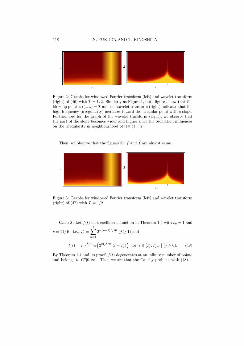
Figure 2: Graphs for windowed Fourier transform (left) and wavelet transform(right) of (46) with T = 1/2. Similarly as Figure 1, both figures show that theblow-up point is t(≡ b) = T and the wavelet transform (right) indicates that thehigh frequency (irregularity) increases toward the irregular point with a slope.Furthermore for the graph of the wavelet transform (right), we observe thatthe part of the slope becomes wider and higher since the oscillation influenceson the irregularity in neighbourhood of t(≡ b) = T .

Then, we observe that the figures for f and f are almost same.

Figure 3: Graphs for windowed Fourier transform (left) and wavelet transform(right) of (47) with T = 1/2.

Case 3: Let f(t) be a coefficient function in Theorem 1.4 with s0 = 1 and

s = 11/10, i.e., Tj =j∑

n=1

2−(n−1)2/20 (j ≥ 1) and

f(t) = 2−j2/10Θ

(221j2/20(t− Tj)

)for t ∈ [Tj , Tj+1] (j ≥ 0). (48)

By Theorem 1.4 and its proof, f(t) degenerates at an infinite number of pointsand belongs to C0[0,∞). Then we see that the Cauchy problem with (48) is


G11/10 ill-posed. For the ill-posedness it is possible to replace the function (48)by

f(t) = 2−jr/10Θ(211jr/20(t− Tj)

with r > 1 (see Remark 2.14). It is not so difficult to describe the figure ofthe wavelet transform even for a large r. Meanwhile, as r is larger, it would bemore difficult to describe the figure of the windowed Fourier transform. For thesimplicity, supposing that r = 1, we shall describe the figures of the following:

Tj =j∑

n=1

2−(n−1)/20 (j ≥ 1)

andf(t) = 2−j/10Θ

(221j/20(t− Tj)

)for t ∈ [Tj , Tj+1] (j ≥ 0). (49)

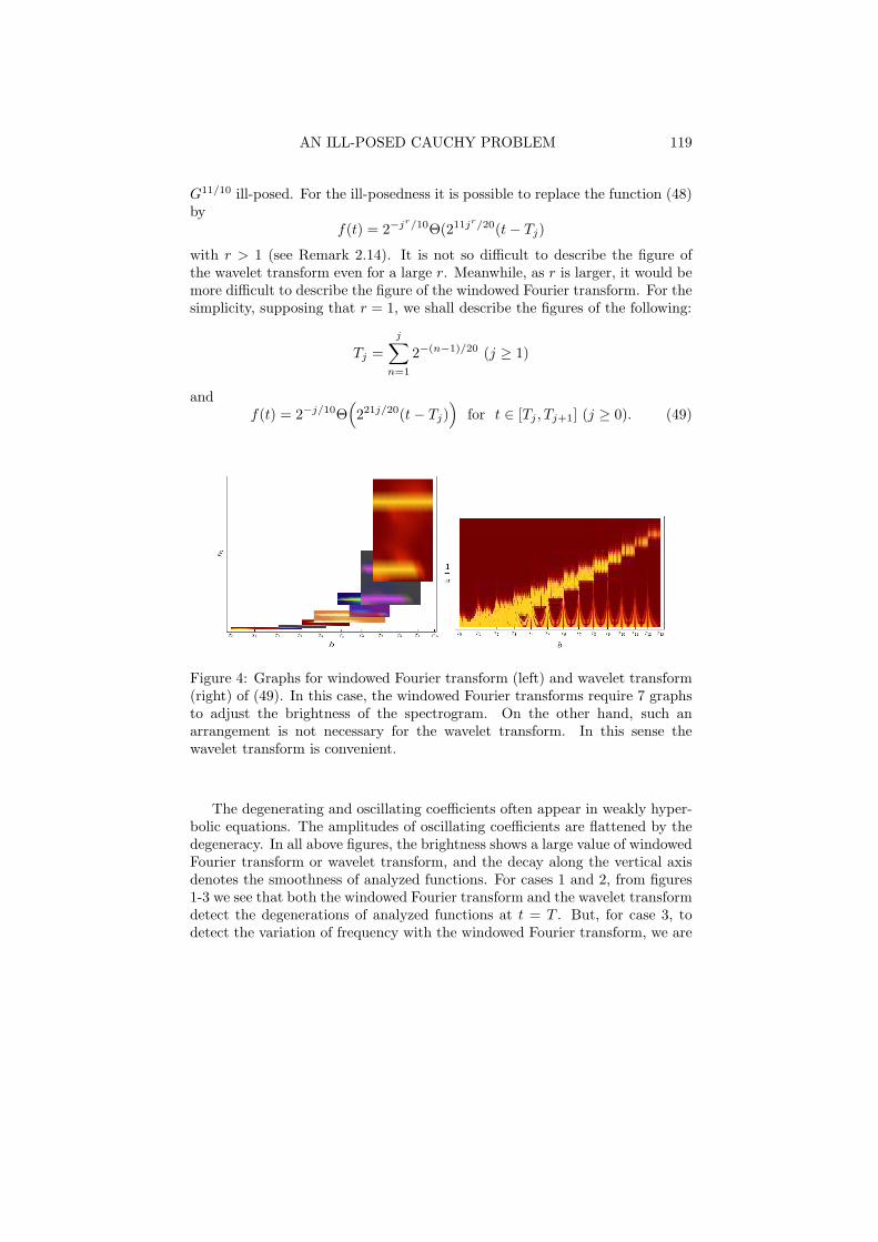
Figure 4: Graphs for windowed Fourier transform (left) and wavelet transform(right) of (49). In this case, the windowed Fourier transforms require 7 graphsto adjust the brightness of the spectrogram. On the other hand, such anarrangement is not necessary for the wavelet transform. In this sense thewavelet transform is convenient.

The degenerating and oscillating coefficients often appear in weakly hyper-bolic equations. The amplitudes of oscillating coefficients are flattened by thedegeneracy. In all above figures, the brightness shows a large value of windowedFourier transform or wavelet transform, and the decay along the vertical axisdenotes the smoothness of analyzed functions. For cases 1 and 2, from figures1-3 we see that both the windowed Fourier transform and the wavelet transformdetect the degenerations of analyzed functions at t = T . But, for case 3, todetect the variation of frequency with the windowed Fourier transform, we are


forced to prepare some graphs according to the value of the windowed Fouriertransform (its graph is obtained by pasting together). On the other hand, thewavelet transform is able to catch more information of low amplitudes withhigh-frequency oscillations in comparison with the windowed Fourier trans-form. Moreover, the multiplication by 1/

√a in the definition of wavelet (44)

makes the amplitudes more conspicuous. The slopes of figures in case 3 in-dicate that a peak moves toward the blow-up point T > 0 as the frequencyincreases, which possibly causes the ill-posedness. Thus, the wavelet transformcan be used as a good screening test for coefficients giving the ill-posedness ofthe Cauchy problem.

Remark 2.21. Generally for a function f(t) = F(t−b′a′

), the wavelet transform

with ψ(t−ba

)detects a ∼ a′ and b ∼ b′. Figure 4 means that a ∼ 2−21j/20 and

b = Tj are conspicuous since f(t) = 20−j/10Θ(

t−Tj

2−21j/20

).

References

[1] F. Colombini, D. Del Santo and T. Kinoshita, Well-posedness of theCauchy problem for a hyperbolic equation with non-Lipschitz coefficients, Ann.Sc. Norm. Super. Pisa, 1 (2002), 327–358.

[2] F. Colombini, D. Del Santo and T. Kinoshita, Gevrey-well-posedness forweakly hyperbolic operators with non-regular coefficients, J. Math. Pures Appl.,81 (2002), 641–654.

[3] F. Colombini, E. De Giorgi and S. Spagnolo, Sur les equations hyperboliquesavec des coefficients qui ne dependent que du temps, Ann. Sc. Norm. Super. Pisa6, 511–559 (1979).

[4] F. Colombini, E. Jannelli and S. Spagnolo, Wellposedness in the Gevreyclasses of the Cauchy problem for a non strictly hyperbolic equation with coeffi-cients depending on time, Ann. Sc. Norm. Super. Pisa 10, 291–312 (1983).

[5] F. Colombini and S. Spagnolo, An example of a weakly hyperbolic Cauchyproblem not well posed in C∞, Acta Math. 148, 291–312 (1982).

[6] P. D’Ancona, Gevrey well posedness of an abstract Cauchy problem of weaklyhyperbolic type, Publ. RIMS Kyoto Univ. 24, 243–253 (1988).

[7] T. Kinoshita and M. Reissig, The log-effect for 2 by 2 hyperbolic systems, J.Differential Equations 248, 470–500 (2010).

[8] S. Mizohata, On the Cauchy problem, Notes and Reports in Mathematics inScience and Engineering, 3. Academic Press, Inc., Orlando, FL; Science Press,Beijing, 1985.


[9] T. Nishitani, Sur les equations hyperboliques a coefficients holderiens en t et declasses de Gevrey en x, Bull. Sci. Math. 107, 113–138 (1983).

Authors’ addresses:

Naohiro FukudaInstitute of Mathematics, University of Tsukuba,Tsukuba Ibaraki 305-8571, JapanE-mail: [email protected]

Tamotu KinoshitaInstitute of Mathematics, University of Tsukuba,Tsukuba Ibaraki 305-8571, JapanE-mail: [email protected]

Received May 16, 2013Revised September 12, 2013

Documents

On a coeﬃcient concerning an ill-posed Cauchy problem and ... · Cauchy problem and the singularity detection with the wavelet transform Naohiro Fukuda and Tamotu Kinoshita Abstract