Lecture notes on transport equation and

Cauchy problem for BV vector

�elds and applications

Luigi Ambrosio

Scuola Normale Superiore

Piazza dei Cavalieri 7, 56126 Pisa, Italy

l.ambrosio@sns.it

1 Introduction

PROPRIETA' DI SEMIGRUPPO

In these notes I would like to describe informally the main results obtained in [6],

together with some recent improvements. In that paper I study the well posedness of the

continuity equation and of the ODE for vector �elds b(t; x) having a low regularity with

respect to the spatial variables, precisely a BV (bounded variation) regularity. These

results extend the DiPerna{Lions theory, in which a Sobolev regularity was considered.

The extension to BV vector �elds is crucial in view of the application, described in the

last paragraph, to a particular system of conservation law considered by Bressan in [13]

and then in two papers of mine [7], [8], the �rst one written with De Lellis and the second

one with Bouchut and De Lellis.

The problem can be presented from two di�erent viewpoints, an Eulerian one and

a Lagrangian one one. We will see that there is indeed a close link between the two

viewpoints.

Let b : [0; T ] � Rd ! Rd be a Borel vector �eld. The Eulerian problem is the well-

posedness of

(PDE) _�t +Dx � (b�t) = 0; �0 = Ld A; t 2 [0; T ]

(here _�t stands for time derivative), where �t is a suitable time-depending family of

measures, possibly signed. In all situations that we will consider there will be bounds on

b and/or �t ensuring thatZI

�j�tj(BR) +

ZBR

jbj dj�tj

�dt 8I �� (0; T ); R > 0;

1

so that the PDE will make sense in the sense of distributions in (0; T )� Rd .

The Lagrangian problem is the uniqueness of

(ODE)

�_ (t) = b (t; (t))

(0) = x:

In some situations one might hope for a \generic" uniqueness of the solutions of ODE,

i.e. for \almost every" initial datum x. An even weaker requirement is the research of a

\selection principle", i.e. a strategy to select for almost every x a solution (�; x) in such

a way that this selection is stable w.r.t. smooth approximations of b. In other words,

we would like to know that, whenever we approximate b by smooth vector �elds bh, the

classical trajectiories associated to bh satisfy

limh!1

h(�; x) = (�; x) in C([0; T ];Rd), for a.e. x.

In these notes I will consider only the forward problem (this allows to state sharper

one-sided conditions on the divergence of the vector �elds involved) and a bounded time

interval [0; T ]. With the simple necessary adaptations more general time intervals could

be considered as well.

Finally, I conclude this short introduction with some bibliographical remarks, that

do not pretend to be exhaustive. The �rst paper where the connection between the

Lagrangian and the Eulerian viewpoint is investigated in detail, in a weak setting, is due

to DiPerna{Lions [24], that consider a Sobolev dependence (precisely proving uniqueness

of Lq solutions of the PDE for W 1;p vector�elds, 1 � p � 1), and in [29] Lions extended

these results to the piecewise Sobolev case. In [14] Capuzzo Dolcetta and Perthame

proved, among other things, that the DiPerna{Lions theiry still works assuming only

that the simmetric part of the distributional derivative is in L1loc (no assumption on the

antisymmetric part, that could be only a distribution). In this connection it is also

worth to mention the papers [15], [16] by Cellina and Cellina{Vornicescu, that study the

di�erential inclusion _ (t) 2 A ( (t)), with A maximal monotone. In this case uniqueness

of the ODE holds for L d-a.e. initial datum x.

A fundamental paper is due to Bouchut [12], where the problem is solved for II order

equation 00(t) = b (t; (t)) and, more generally, for some equations of Hamiltonian type.

In the paper [17] (see also [18]) Colombini{Lerner consider a particular class of BV vector

�elds, that they call co-normal BV vector �elds, that reduce to vector �elds analogous to

Bouchut's ones after a (local) bi-Lipschitz change of coordinates. Finally, in [6] I got the

general case, imposing only BV regularity and absolute continuity of the divergence with

respect to L d.

The literature in this area is very wide, due to the fundamental character of the

continuity equation, and the enclosed bibliography is far from being exhaustive. In any

case I wish to mention also the papers [27], [28], containing other uniqueness results in the

2

2-dimensional case, and the papers [31], [11], where generalized characteristics and one-

sided Lipschitz conditions on the vector �eld are taken into account (for characteristics

in the non-linear setting of conservation laws, see also [22]).

I believe that we are still quite far from a good understanding of the optimal conditions

on the vector �eld b, but there are some counterexamples, that for the sake of brevity I

will not discuss, showing which phenomena can prevent the uniqueness: besides the two

counterexamples in [24], I recall also the papers [1], [19], [23].

2 The classical setup: b 2 L1�[0; T ];W 1;1(R d)

�

Under this assumption it is well known that solutions X(t; �) of the ODE are unique and

stable. A quantitative information can be obtained by di�erentiation:

d

dtjX(t; x)�X(t; y)j2 � 2krbtk1jX(t; x)�X(t; y)j2;

so that Gronwall lemma immediately gives

Lip (X(t; �)) � exp

�Z t

0

krbsk1 ds

�: (2.1)

Turning to the solutions of the ODE, uniqueness will be proved in a more general set-

ting for positive measure-valued solutions (via the superposition principle) and for signed

solutions (via the theory of renormalized solutions), so here we focus on the existence and

the representation issue. The representation formula is indeed very simple

�t := X(t; �)#�� (2.2)

and we need only to check it. Notice �rst that we need only to check the distributional

identity on test functions of the form (t)'(x), so thatZR

0(t)h�t; 'i+

ZR

(t)

ZRd

hbt;r'i d�t dt = 0:

This means that we have to check that t 7! h�t; 'i belongs to W1;1(0; T ) for any ' 2

C1c (Rd) and that its distributional derivative is

RRdhbt;r'i d�t.

We show �rst that the map is absolutely continuous, and in particular W 1;1(0; T );

then one needs only to compute the pointwise derivative. For every choice of �nitely

many pairwise disjoint intervals (ai; bi) � [0; T ] we have

nXi=1

jX(bi; x)�X(ai; x)j �

Z[i(ai;bi)

j _X(t; )j dt �

Z[i(ai;bi)

krbtk1 dt

3

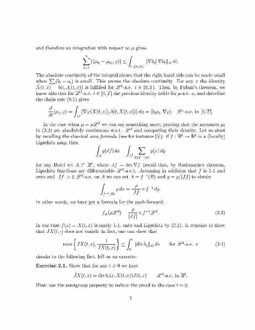
and therefore an integration with respect to �� gives

nXi=1

jh�bi � �ai ; 'ij �

Z[i(ai;bi)

krbtkrbtk1 dt:

The absolute continuity of the integral shows that the right hand side can be made small

whenP

i(bi � ai) is small. This proves the absolute continuity. For any x the identity_X(t; x) = b(t; X(t; x)) is ful�lled for L 1-a.e. t 2 [0; T ]. Then, by Fubini's theorem, we

know also that forL 1-a.e. t 2 [0; T ] the previous identity holds for �-a.e. x, and therefore

the chain rule (8.1) gives

d

dth�t; 'i =

ZRd

hr'(X(t; x)); b(t; X(t; x))i d� = hbt�t;r'i L1-a.e. in [0; T ]:

In the case when �� = �L d we can say something more, proving that the measures �tin (2.2) are absolutely continuous w.r.t. L d and computing their density. Let us start

by recalling the classical area formula (see for instance [5]): if f : Rd ! Rd is a (locally)

Lipschitz map, then ZA

gjJf j dx =

ZRd

Xx2f�1(y)

g(x) dy

for any Borel set A � Rd , where Jf = detrf (recall that, by Rademacher theorem,

Lipschitz functions are di�erentiable L d-a.e.). Assuming in addition that f is 1-1 and

onto and jJf j > 0 L d-a.e. on A we can set A = f�1(B) and g = �=jJf j to obtainZf�1(B)

� dx =�

jJf jÆ f�1 dy:

In other words, we have got a formula for the push-forward:

f#(�Ld) =

�

jJf jÆ f�1

Ld: (2.3)

In our case f(x) = X(t; x) is surely 1-1, onto and Lipschitz by (2.1). It remains to show

that JX(t; �) does not vanish: in fact, one can show that

max

�JX(t; x);

1

JX(t; x)

��

Z t

0

kdiv bsk1 ds for L d-a.e. x (2.4)

thanks to the following fact, left as an exercise.

Exercise 2.1. Show that for any t � 0 we have

_JX(t; x) = div bt(x;X(t; x))J(t; x) Ld-a.e. in Rd .

Hint: use the semigroup property to reduce the proof to the case t = 0.

4

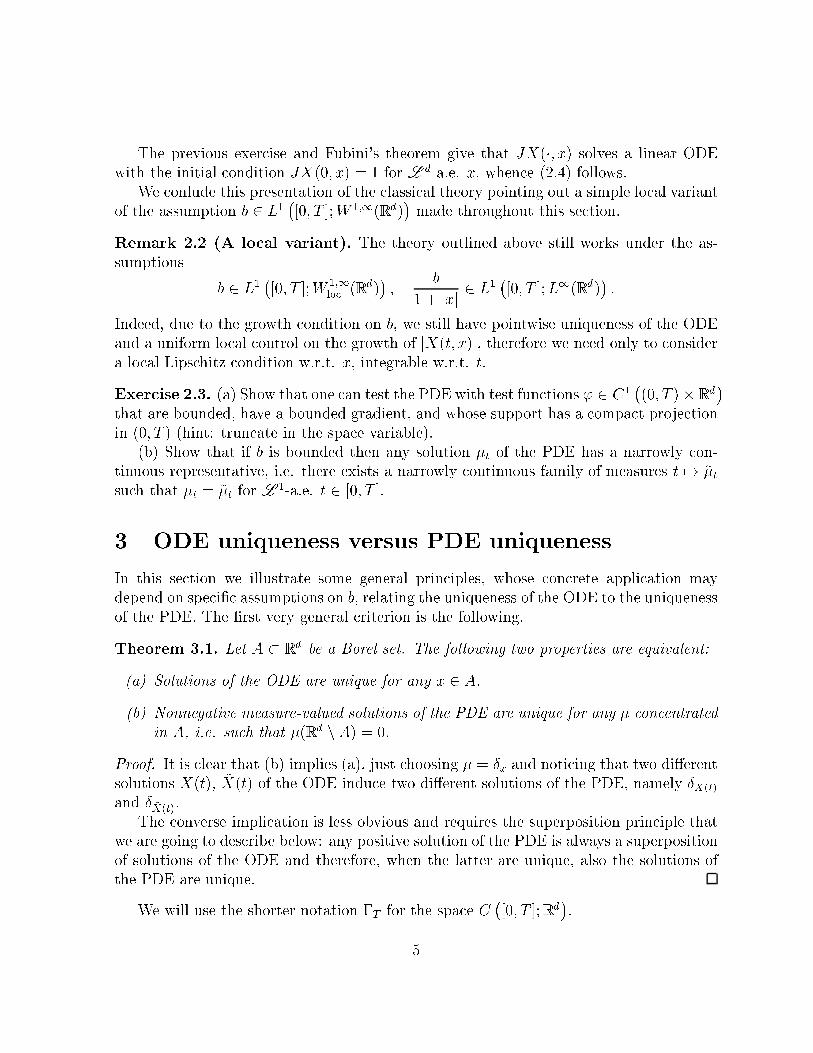
The previous exercise and Fubini's theorem give that JX(�; x) solves a linear ODE

with the initial condition JX(0; x) = 1 for L d-a.e. x, whence (2.4) follows.

We conlude this presentation of the classical theory pointing out a simple local variant

of the assumption b 2 L1�[0; T ];W 1;1(Rd)

�made throughout this section.

Remark 2.2 (A local variant). The theory outlined above still works under the as-

sumptions

b 2 L1�[0; T ];W

1;1loc (Rd)

�;

b

1 + jxj2 L1

�[0; T ];L1(Rd)

�:

Indeed, due to the growth condition on b, we still have pointwise uniqueness of the ODE

and a uniform local control on the growth of jX(t; x)j, therefore we need only to consider

a local Lipschitz condition w.r.t. x, integrable w.r.t. t.

Exercise 2.3. (a) Show that one can test the PDE with test functions ' 2 C1�(0; T )� Rd

�that are bounded, have a bounded gradient, and whose support has a compact projection

in (0; T ) (hint: truncate in the space variable).

(b) Show that if b is bounded then any solution �t of the PDE has a narrowly con-

tinuous representative, i.e. there exists a narrowly continuous family of measures t 7! ~�tsuch that �t = ~�t for L

1-a.e. t 2 [0; T ].

3 ODE uniqueness versus PDE uniqueness

In this section we illustrate some general principles, whose concrete application may

depend on speci�c assumptions on b, relating the uniqueness of the ODE to the uniqueness

of the PDE. The �rst very general criterion is the following.

Theorem 3.1. Let A � Rd be a Borel set. The following two properties are equivalent:

(a) Solutions of the ODE are unique for any x 2 A.

(b) Nonnegative measure-valued solutions of the PDE are unique for any �� concentrated

in A, i.e. such that ��(Rdn A) = 0.

Proof. It is clear that (b) implies (a), just choosing �� = Æx and noticing that two di�erent

solutions X(t); ~X(t) of the ODE induce two di�erent solutions of the PDE, namely ÆX(t)

and Æ ~X(t).

The converse implication is less obvious and requires the superposition principle that

we are going to describe below: any positive solution of the PDE is always a superposition

of solutions of the ODE and therefore, when the latter are unique, also the solutions of

the PDE are unique.

We will use the shorter notation �T for the space C�[0; T ];Rd

�.

5

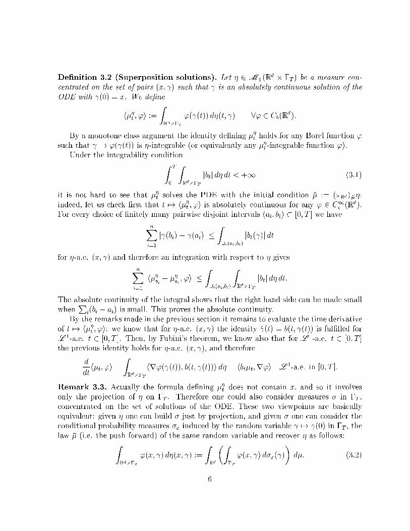
De�nition 3.2 (Superposition solutions). Let � 2 M+(Rd � �T ) be a measure con-

centrated on the set of pairs (x; ) such that is an absolutely continuous solution of the

ODE with (0) = x. We de�ne

h��t ; 'i :=

ZRd��T

'( (t)) d�(t; ) 8' 2 Cb(Rd):

By a monotone class argument the identity de�ning ��t holds for any Borel function '

such that 7! '( (t)) is �-integrable (or equivalently any ��t -integrable function ').

Under the integrability conditionZ T

0

ZRd��T

jbtj d� dt < +1 (3.1)

it is not hard to see that ��t solves the PDE with the initial condition �� := (�Rd)#�:

indeed, let us check �rst that t 7! h��t ; 'i is absolutely continuous for any ' 2 C1c (Rd).

For every choice of �nitely many pairwise disjoint intervals (ai; bi) � [0; T ] we have

nXi=1

j (bi)� (ai)j �

Z[i(ai;bi)

jbt( )j dt

for �-a.e. (x; ) and therefore an integration with respect to � gives

nXi=1

jh��bi � ��ai; 'ij �

Z[i(ai;bi)

ZRd��T

jbtj d� dt:

The absolute continuity of the integral shows that the right hand side can be made small

whenP

i(bi � ai) is small. This proves the absolute continuity.

By the remarks made in the previous section it remains to evaluate the time derivative

of t 7! h��t ; 'i: we know that for �-a.e. (x; ) the identity _ (t) = b(t; (t)) is ful�lled for

L 1-a.e. t 2 [0; T ]. Then, by Fubini's theorem, we know also that for L 1-a.e. t 2 [0; T ]

the previous identity holds for �-a.e. (x; ), and therefore

d

dth�t; 'i =

ZRd��T

hr'( (t)); b(t; (t))i d� = hbt�t;r'i L1-a.e. in [0; T ]:

Remark 3.3. Actually the formula de�ning ��t does not contain x, and so it involves

only the projection of � on �T . Therefore one could also consider measures � in �T ,

concentrated on the set of solutions of the ODE. These two viewpoints are basically

equivalent: given � one can build � just by projection, and given � one can consider the

conditional probability measures �x induced by the random variable 7! (0) in �T , the

law �� (i.e. the push forward) of the same random variable and recover � as follows:ZRd��T

'(x; ) d�(x; ) :=

ZRd

�Z�T

'(x; ) d�x( )

�d��: (3.2)

6

Our viewpoint has been chosen just for technical convenience, to avoid the use, wherever

this is possible, of the conditional probability theorem.

By restricting � to suitable subsets of Rd��T , several manipulations with superposition

solutions of the continuity equation are possible and useful, and these are not immediate

to see at the level of general solutions of the continuity equation. This is why the following

result is interesting (although it plays a little role in these notes, unlike the concept of

superposition solution).

Theorem 3.4 (Superposition principle). Let �t 2 M+(Rd) solve PDE and assume

thatR T0kbtkL1(�t) dt < +1. Then �t is a superposition solution, i.e. there exists � 2

M+(Rd � �T ) such that �t = ��t for any t 2 [0; T ].

Proof. Here we just a hint of the proof, referring to Chapter 9 of [9] for a detailed one.

We mollify �t w.r.t. the space variable with a Gaussian kernel � (or any other kernel

whose support is the whole space), obtaining smooth and strictly positive functions ��t.

De�ning

b�t :=(bt�t) � ��

��t

it is immediate that

_��t +D � (b�t��t) = 0

and b�t is locally Lipschitz w.r.t. x, with a suÆcient uniformity w.r.t. t, so that the

representation ��t = X�(t; �)#��0. Then, we de�ne

�� := (x;X�(�; x))# ��0

so that ZRd��T

'( (t)) d�� =

ZRd

'(X�(t; x)) d��0(x) =

ZRd

'd��t: (3.3)

Since ZRd��T

Z T

0

j _ j dt d��(x; ) =

Z T

0

ZRd

jb�tj d��t dt �

Z T

0

kbtkL1(�t) dt

and the length functional has compact sublevels in �T , Prokhorov theorem tells us that

the family �� is tight as � # 0, and if � is any limit point we can pass to the limit in (3.3)

to obtain that �t = ��t . The more delicate part of the proof is the �nal one, where it is

shown that � is concentrated on the solutions of the ODE.

The applicability of Theorem 3.1 is strongly limited by the fact that pointwise unique-

ness properties are known only in very special situations, for instance when there is a

Lipschitz or a one-sided Lipschitz condition. It turns out that in many cases uniqueness

7

of the PDE can only be proved in smaller classes L of solutions, and it is natural to think

that this should re ect into a weaker uniqueness condition at the level of the ODE.

We will see indeed that there is uniqueness in the \selection sense". In order to

illustrate this concept, in the following we consider a convex class L of measure-valued

solutions �t 2M+(Rd) of the PDE, satifying the following monotonicity property:

0 � �0t � �t 2 L =) �0t 2 L : (3.4)

The typical application will be with absolutely continuous measures �t, whose densities

satisfy some quantitative and possibly time-depending bound.

De�nition 3.5 (L -lagrangian ows). Given the class L , we say that X(t; x) is a

L -Lagrangian ow starting from �� if the following two properties hold:

(a) X(�; x) solves the ODE for ��-a.e. x;

(b) �t := X(t; �)#�� 2 L .

HeuristicallyL -Lagrangian ows can be thought as suitable selections of the solutions

of the ODE (possibly non unique), made in such a way to produce a density in L . The

following theorem shows that the L -Lagrangian ow starting from �� is unique, modulo

��-negligible sets, whenever a comparison principle for the PDE holds, in the class L . We

will show existence (and stability) in the Sobolev or BV context in the next sections: in

these cases the measure �� is absolutely continuous w.r.t. L d.

Theorem 3.6 (Uniqueness). Assume that the PDE ful�ls the comparison principle in

L . Then the L -Lagrangian ow starting from �� is unique, i.e. two di�erent selections

X(t; x) and ~X(t; x) of solutions of the ODE producing solutions of the PDE in L satisfy

X(�; x) = ~X(�; x) in �T for ��-a.e. x.

Proof. If the statement is false we can produce a measure � not concentrated on a graph

inducing a solution ��t 2 L of the PDE. This is not possible, thanks to the next result.

The measure � can be built as follows:

� :=1

2

�(x;X(�; x))#��+ (x; ~X(�; x))#��

�:

Since L is convex we still have ��t 2 L .

Theorem 3.7. Assume that the PDE ful�ls the comparison principle in L . Let � 2

P(Rd � �T ) be as in De�nition 3.2 and assume that ��t 2 L . Then � is concentrated on

a graph, i.e. there exists a function x 7! X(�; x) 2 �T such that

� =�x;�(�; x)

�#��; with �� := (�Rd)#� = ��0:

8

Proof. We use the representation (3.2) of �, given by the disintegration theorem, the

criterion stated in Lemma 3.9 below and argue by contradiction. If the thesis is false then

�x is not a Dirac mass in a set of �� positive measure and we can �nd t 2 (0; T ], disjoint

Borel sets E; E 0 � Rd and a Borel set C with ��(C) > 0 such that

�x (f : (t) 2 Eg) �x (f : (t) 2 E 0g) > 0 8x 2 C:

Possibly passing to a smaller set having still strictly positive �� measure we can assume

that

0 < �x(f : (t) 2 Eg) �M�x(f : (t) 2 E 0g) 8x 2 C (3.5)

for some constant M . We de�ne measure-valued maps �1; �2 by

�1x := � f(x; ) : x 2 C; (t) 2 Eg; �2x :=M� f(x; ) : x 2 C; (t) 2 E 0g

and denote by �it the superposition solutions induced by �i. Then

�10 = �tx(E)�� C; �20 =M�tx(E0)�� C;

so that (3.5) yields �10 � �20. On the other hand

�1t =

ZC

�tx E d�(x) ?M

ZC

�tx E 0 d�(x) = �2t :

Notice also that �it � �t and so the monotonicity assumption (3.4) on L gives �it 2 L .

This contradicts the assumption on the validity of the comparison principle in L .

Exercise 3.8. Let � 2M+(X) and let D � [0; T ] be a dense set. Show that � is a Dirac

mass in �T i� its projections (t)#�, t 2 D, are Dirac masses in Rd .

Lemma 3.9. Let �x be a measurable family of positive �nite measures in �T with the

following property: for any t 2 [0; T ] and any pair of disjoint Borel sets E; E 0 � Rd we

have

�x (f : (t) 2 Eg) �x (f : (t) 2 E 0g) = 0 ��-a.e. in Rd . (3.6)

Then �x is a Dirac mass for ��-a.e. x.

Proof. Taking into account Exercise 3.8, for a given t 2 (0; T ] it suÆces to check that the

measures �x := (t)#�x are Dirac masses for ��-a.e. x. Then (3.6) gives �x(E)�x(E0) = 0

��-a.e. for any pair of disjoint Borel sets E; E 0 � Rd . Let Æ > 0 and let us consider

a partition of Rd in countably many sets Ri having a diameter less then Æ. Then, as

�x(Ri)�x(Rj) = 0 �-a.e. whenever i 6= j, we have a corresponding decomposition of

��-almost all of Rd in Borel sets Ai such that supp�x � Ri for any x 2 Ai (just take

f�x(Ri) > 0g and subtract from him all other sets f�x(Rj) > 0g, j 6= i). Since Æ is

arbitrary the statement is proved.

9

4 The DiPerna{Lions theory

The key ingredient of the theory is the concept of renormalized solution. Before intro-

ducing this concept, we de�ne the distribution b � rw in (0; T )� Rd as follows

hbrw; 'i := �

Zwhb;r'idtdx�

Z T

0

hDx � bt; wt'ti dt:

Notice that this is consistent with the case when w is smooth, and that the second integral

makes sense only when Dx � bt � Ld for L 1-a.e. t 2 (0; T ).

De�nition 4.1 (Renormalized solutions). Let b 2 L1loc

�(0; T );L1

loc(Rd)�be such that

D � bt = div btLd for L 1-a.e. t 2 (0; T ), with

div bt 2 L1loc

�(0; T );L1

loc(Rd)�: (4.1)

Let w 2 L1loc�(0; T );L1(Rd)

�and assume that

c :=d

dtw + b � rw 2 L1

loc

�(0; T )� Rd

�: (4.2)

Then, we say that w is a renormalized solution if

d

dtw + b � rw = c� 0(w) 8� 2 C1(R):

One of the main results of [24] states that under a Sobolev regularity assumption on

bt any distributional solution is in fact also a renormalized one.

Theorem 4.2 (Renormalization theorem). Let b as in De�nition 4.1 and assume in

addition that

b 2 L1loc

�(0; T );W

1;1loc (R

d)�:

Then any distributional solution of (4.2) is a renormalized solution.

Proof. We mollify with respect to the spatial variables and we set

r� := (brw) � �� � b � (r(w � ��)); w� := w � ��

to obtain

_w� + b � rw� = c � �� + r�:

By the smoothness of w� w.r.t. x, the PDE above tells that _w�t 2 L1

loc, therefore w� 2

W 1;1loc

�(0; T )� Rd

�and we can apply the standard chain rule in Sobolev spaces, getting

_�(w�) + b � r�(w�) = � 0(w�)c � �� + � 0(w�)r�:

10

When we let � # 0 the convergence in the distribution sense of all terms in the identity

above is trivial, with the exception of the last one. To ensure its convergence to zero, it

seems necessary to show that r� ! 0 strongly in L1loc (remember that � 0(w�) is locally

equibounded w.r.t. �). This strong convergence of the \commutators" r� can be achieved

as follows. Playing with the de�nitions of b�rw and convolution product of a distribution,

one proves �rst the identity

r�(t; x) =

ZRd

w(t; x� �y)bt(x� �y)� bt(x)

�dy � (wdiv bt) � ��(t; x): (4.3)

Then, one uses the strong convergence of translations in Lp and the strong convergence

of the di�erence quotients (a property that characterizes functions in Sobolev spaces)

u(x+ �z)� u(x)

�! ru(x)z strongly in L1

loc, for u 2 W1;1loc

to obtain that r� strongly converges in L1loc to

�w(t; x)

ZRd

hrbt(x)y;r�(y)i dy� w(t; x)div bt(x):

The elementary identity ZRd

yi@�

@yjdy = �Æij (4.4)

then shows that the limit is 0 (this can also be derived by the fact that, in any case, the

limit of r� in the distribution sense is 0).

Using the renormalization teorem we can prove a comparison principle in the class L

de�ned below.

L :=�w 2 L1

�[0; T ];L1(Rd)

�\ L1

�[0; T ];L1(Rd)

�: w 2 C

�[0; T ];w�

� L1(Rd)�:

(4.5)

Theorem 4.3 (Comparison principle). Assume that

b

1 + jxj2 L1

�[0; T ];L1(Rd)

�+ L1

�[0; T ];\L1(Rd)

�; (4.6)

that D � bt = div btLd for L 1-a.e. t 2 [0; T ], and thatZ T

0

k[div bt]�k1 dt < +1: (4.7)

Assume in addition that any solution of (4.2) is renormalized. Then the comparison

principle holds in the class L de�ned in (4.5).

11

Proof. By the linearity of the equation, it suÆces to show that w 2 L and w(0; �) � 0

implies wt � 0 for any t 2 [0; T ]. We extend �rst the PDE to negative times, setting wt =

w0 and bt = 0 for t � 0. Then, �x a cut-o� function � 2 C1c (Rd) with supp' � B2(0)

and ' � 1 on B1(0), and the renormalization function

�(t) :=p1 + (t+)2 � 1 2 C1(R):

Notice that � is convex, that �(t) = 0 i� t � 0 and that �(t) � t for any t 2 R. We know

thatd

dt�(wt) +Dx � �(wt) = div bt(�(wt)� wt�

0(wt))

in the sense of distributions in R�R d , and clearly �(wt) = 0 L d+1-a.e. on (�1; 0)�Rd .

Plugging 'R(�) := '(�=R), with R � 1, into the PDE we obtain

d

dt

ZRd

'R�(wt) dx

ZRd

�(wt)hbt;r'Ri dx+

ZRd

'Rdiv bt(�(wt)� wt�0(wt)) dx:

Splitting b as b1 + b2, with

b1

1 + jxj2 L1

�[0; T ];L1(Rd)

�and

b2

1 + jxj2 L1

�[0; T ];L1(Rd)

�and using the inequality

1

R�R�jxj�2R �

3

1 + jxj�R�jxj

we can estimate the �rst integral in the right hand side with

3kr'k1kb1t

1 + jxjk1

Zjxj�R

jwtj dx+ 3kr'k1kwtk1

Zjxj�R

jb1tj

1 + jxjdx:

The second integral can be estimated with

k[div bt]�k1

ZRd

'R�(wt) dx;

taking into account that 0 � t� 0(t)� �(t) � �(t).

These inequalities have to be understood in the sense of distributions in R, since we

don't know a priori if t 7! �(wt) is continuous or not. Passing to the limit as R!1 and

using the integrability assumption on b we get

d

dt

ZRd

�(wt) dx � k[div bt]�k1

ZRd

�(wt) dx

in the distribution sense in R. Since the function vanishes for negative times, this suÆces

to conclude using Gronwall lemma and (4.7).

12

5 BV dependence with respect to the spatial vari-

ables

One of the main results of [6] is the following one, where we obtain the renormalization

lemma under a BV dependence w.r.t. the spatial variables (but still assuming that

D � bt � Ld for L 1-a.e. t 2 (0; T )).

Theorem 5.1. Let b as in De�nition 4.1 and assume in addition that

b 2 L1loc

�(0; T );BVloc(R

d)�:

Then any distributional solution of (4.2) is a renormalized solution.

This section is devoted to a reasonably detailed proof of this result. Before doing that

we set up some notation, denoting by

Dbt = rbtLd +Dsbt

the Radon{Nikodym decomposition of Dbt in absolutely continuous and singular part

w.r.t. L d. We also introduce the measures jDbj and jDsbj by integration w.r.t. the time

variable, i.e.Z'(t; x) djDbj :=

Z T

0

ZRd

'(t; x) djDbtj dt;

Z'(t; x) djDsbj :=

Z T

0

ZRd

'(t; x) djDsbtj dt:

Let us start from the expression (4.3) of the commutators: since b(t; �) =2 W 1;1 we

cannot use the strong convergence of the di�erence quotients, as done in [24]. However,

for any function u 2 BVloc and any z 2 Rd we have the classical L1 estimate on the

di�erence quotients (see for instance [5])ZK

ju(x+ z)� u(x)j dx � jDzuj(K�) for any K � Rd compact,

where Du = (D1u; : : : ; Ddu) stands for the distributional derivative of u, Dzu = hDu; zi =Pi ziDiu denotes the component along z of Du and K� is the open �-neighbourhood of

K. We notice that

Dzhbt;r�(z)i = hMt(�)z;r�(z)ijDbj

and therefore the L1 estimate on di�erence quotients gives

lim sup�#0

ZK

jr�j dx � kwk1

ZK

ZRd

jhMt(x)z;r�(z)ij dzdjDbj(t; x) (5.1)

for any compact set K � (0; T )� Rd .

13

On the other hand, a di�erent estimate of the commutators that reduces to the stan-

dard one when b(t; �) 2 W1;1loc can be achieved as follows. Let us start from the case d = 1:

if � is a Rm -valued measure in R with locally �nite variation, then by Fubini's theorem

the functions

�̂�(t) :=�([t; t+ �])

�= � �

�[��;0]]

�(t); t 2 R

satisfy ZK

j�̂�j dt � j�j(K�) for any compact set K � R ; (5.2)

whereK� is the open � neighbourhood ofK. A density argument based on (5.2) then shows

that �̂� converge in L1loc(R) to the density of � with respect to L 1 whenever �� L 1. If

u 2 BVloc and � > 0 we know that

u(x+ �)� u(x)

�=Du([x; x+ �])

�=Dau([x; x+ �])

�+Dsu([x; x+ �])

�

for L 1-a.e. x (the exceptional set possibly depends on �). In this way we have split the

di�erence quotient, as the sum of two functions, one strongly converging to ru in L1loc,

and the other one having an L1 norm on any compact set K asymptotically smaller than

jDsuj(K).

If we �x the direction z of the di�erence quotient, the slicing theory of BV functions

(see [5]) gives that this decomposition can be carried on also in d-dimensions, showing

that the di�erence quotientsbt(x� �z) � bt(x)

�

can be canonically split into two parts, the �rst one strongly converging in L1loc(R

d) to

rbt(x)z, and the second one satisfying having an L1 norm on K asymptotically smaller

than jhDsbt; zij(K). Then, repeating the DiPerna{Lions argument and taking into account

the error induced by the presence of the second part of the di�erence quotients we get

lim sup�#0

ZK

jr�j dx � kwk1

ZK

ZRd

jzjjr�(z)j dzdjDsbj(t; x) (5.3)

for any compact set K � (0; T )�Rd . Roughly speaking, the estimate (5.3) is useful in the

regions where the absolutely continuous part is the dominant one, so that jDsbj(K) << 1),

while (5.1) turns out to be useful in the regions where the dominant part is the singular

one. Let us see how the two estimates can be combined: coming back to the smoothing

scheme, we have_�(w�) + b � r�(w�)� � 0(w�)c � �� = � 0(w�)r

� (5.4)

Let us work on an open set A �� (0; T ) � Rd , let L = kwkL1(A) and let L0 be the

supremum of j� 0j on [�M;M ]. Then, (5.3) tells us that limit measure � of j� 0(w�)r�jL d

14

as � # 0 satis�es

� A � LL0I(�)jDsbj with I(�) :=

ZRd

jzjjr�(z)j dz:

In particular � A is singular with respect to L d. On the other hand, the estimate (5.1)

tells also us that

� A � LL0ZRd

jhMt(�)z;r�(z)ij dzjDbj:

These two estimates imply that

� A � LL0ZRd

jhMt(�)z;r�(z)ij dzjDsbj: (5.5)

Notice that in this way we got rid of the potentially dangerous term I(�): in fact, we are

going to choose very anisotropic kernels � on which I(�) can be arbitrarily large. The

measure � can of course depend on the choice of �, but (5.4) tells us that the measure

� :=d

dt�(wt) + b � r�(wt)� etwt�

0(wt);

clearly independent of �, satis�es j�j � � in A. Eventually we obtain

j�j A � LL0�(M�(�); �)jDsbj with �(N; �) :=

ZRd

jhNz;r�(z)ij dz: (5.6)

We are thus led to the minimum problem

G(N) := inf

��(N; �) : � 2 C1

c (B1); � � 0;

ZRd

� = 1

�(5.7)

with N =Mt(x). Notice that (5.6) gives

j�j A � LL0 inf�2D

�(M�(�); �)jDsbj

for any countable setD of kernels �, and the continuity of � 7! �(N; �) w.r.t. theW 1;1(B1)

norm and the separability of W 1;1(B1) give

j�j A � LL0G(M�(�))jDsbj: (5.8)

Notice now that the assumption that D � bt � Ld for L 1-a.e. t 2 (0; T ) gives

traceMt(x)jDsbtj = 0 for L 1-a.e. t 2 (0; T ).

Hence, recalling the de�nition of jDsbj, the trace of Mt(x) vanishes for jDsbj-a.e. (t; x).

Applying the following lemma, due to Alberti [?] 1 and using (5.8) we conclude that � = 0,

concluding the proof.

1Actually this lemma came out during the Luminy school in October of 2003, where I raised theproblem of computing the in�mum in (5.7), and Alberti came up with the solution!

15

Lemma 5.2 (Alberti). For any d� d matrix N the in�mum in (5.7) is jtraceN j.

Proof. Notice �rst that the lower bound follows immediately by the identityZRd

hNz;r�(z)i dz = �traceN;

that in turn follows by (4.4). Hence, we have to show only the upper bound. Since

hNz;r�(z)i = div (Nz�(z)) � traceN�(z)

it suÆces to show that for any T > 0 there exists � such thatZRd

jdiv (Nz�(z))j dz �2

T: (5.9)

The heuristic idea is to build � as the superposition of elementary probability measures

associated to the curves etNx, 0 � t � T , on which the divergence operator can be easily

estimated. Given a smooth kernel � with compact support, it turns out that the function

�(z) :=1

T

Z T

0

�(e�tNz)e�t traceN dt (5.10)

has the required properties (here etNx =P

i tiN ix=i! is the solution of the ODE _ = N

with the initial condition (0) = x). Indeed, it is immediate to check that � is smooth

and compactly supported. To estimate the divergence of Nz�(z), we notice that � =R�(x)�x dx, where �x are the probability 1-dimensional measures concentrated on the

image of the curves t 7! etNx de�ned by

�x := (e�Nx)#(1

TL

1 [0; T ]):

Indeed, for any ' 2 C1c (Rd) we haveZ

Rd

�(x)h�x; 'i dx =1

T

Z T

0

ZRd

�(x)'(etNx) dtdx

=1

T

Z T

0

ZRd

�(e�tNy)e�t traceN'(y) dydt =

ZRd

�(y)'(y) dy:

By the linearity of the divergence operator, it suÆces to check that

jD � (Nz�x)j �2

T8x 2 Rd :

But this is elementary, sinceZRd

hNz;r'(z)i d�x(z) =1

T

Z T

0

hNetNx;r'(etNx)i dt ='(eTNx)� '(x)

T

for any ' 2 C1c (Rd), so that TD � (Nx�x) = Æx � ÆeTNx.

16

We conclude this section noticing that the original argument in [6] is slightly di�erent

and uses, instead of Lemma 5.2, a much deeper result, still due to Alberti [2], saying

that for a BVloc function u : Rd ! Rm the matrix M(x) in the polar decomposition

Du = M jDuj has rank 1 for jDsuj-a.e. x, i.e. there exist unit vectors �(x) 2 Rn and

�(x) 2 Rm such that M(x)z = �(x)hz; �(x)i. In this case the asymptotically optimal

kernels are easy to build, by mollifying in the � direction much faster than in all other

directions (this is precisely what Bouchut did in [12]).

6 Existence and stability of Lagrangian ows

In this section we study the Lagrangian counterpart of the well-posedness results obtained

in the previous two sections, in the Sobolev and in the BV case.

Theorem 6.1 (Existence). Let b 2 L1loc

�(0; T );BVloc(R

d)�be satisfying (4.6) and let us

assume that Dx � bt = div btLd for L 1-a.e. t 2 [0; T ], with k[div bt]

�k1 2 L1(0; T ). Let

L be de�ned as in (4.5) and assume that the comparison principle holds in L +. Then

for any �� = �L d with a nonnegative � 2 L1(Rd) \ L1(Rd) there exists a L d-Lagrangian

ow starting from ��. Moreover, the ow satis�es

X(t; �)#�� � k�k1 exp

�Z t

0

k[div bs]�k1 ds

�L

d: (6.1)

Proof. Step 1. (Smoothing) We de�ne b� = b��� by mollifying with respect to the spatial

variable with a kernel � with compact support, with � 2 (0; 1). Notice thatZ T

0

k[div b�t]�k1 dt �

Z T

0

k[div bt]�k1 dt: (6.2)

Splitting b = (b1 + b2)(1 + jxj) according to (4.6), with

b1 2 L1�[0; T ];L1(Rd)

�; b2 2 L

1�[0; T ];L1(Rd)

�;

we notice that

((1 + jxj)bi) � �� � 2(1 + jxj)(jbij � ��) i = 1; 2

and therefore b� 2 L1�[0; T ];L1(Rd)

�and we can also write b� = b�1 + b�2 with

sup�2(0;1)

kb�1

1 + jxjkL1((0;T );L1(Rd)) < +1; sup

�2(0;1)

kb�2

1 + jxjkL1((0;T );L1(Rd)) < +1; (6.3)

Therefore we can apply Remark 2.2 and consider the characteristics X�(t; x) associated

to b�, together with the induced measures

��t := X�(t; �)#��; �� := (x;X(�; x))# ��

17

with ��t = ���t . Notice also that the explicit representation (2.3) gives

��t = w�tL

d with w�t =

�

JX�(t; �)Æ (X�(t; �))�1 (6.4)

and (2.4) together with (6.2) give

w�t � k�k1 exp

�Z T

0

k[div bs]�k1 ds

�: (6.5)

Step 2. (Tightness of ��) We claim that the family �� is tight: indeed, by the remarks

made after De�nition 8.2, it suÆces to �nd a coercive functional : Rd � �T ! [0;+1)

whose integral w.r.t. all measures �� is uniformly bounded. Since �� has �nite mass we

can �nd a function ' : Rd ! [0;+1) such that ' 2 L1(��) and '(x)! +1 as jxj ! 1.

Then, we de�ne

(x; ) := '(x) + '( (0)) +

Z T

0

j _ j

1 + j jdt

and notice that the coercivity of follows immediately from Lemma 6.2 below. Then,

we compute:

ZRd��T

(x; ) d�� =

ZRd

2'(x) +

Z T

0

j _X�(t; x)j

1 + jX�(t; x)jdt

!d��(x)

= 2

ZRd

' ��+

Z T

0

ZRd

jb�t(X�(t; x))j

1 + jX�(t; x)jd��(x)dt

= 2

ZRd

'd��+

Z T

0

ZRd

jb�tj

1 + jyjw�tdy dt:

Using the uniform L1�(0; T );L1(Rd)

�estimate on w�

t given by (6.5), the uniform L1�(0; T );L1(Rd)

�estimate coming from the fact that w�

t are probability densities and the uniform estimate

(6.3) we conclude that the integrals of are uniformly bounded.

Step 3. (The limit ow belongs toL ) Let now � be a narrow limit point of �� along some

in�nitesimal sequence �i and write �i = ��i in short. Let us show �rst that the induced

ow ��t belongs to L . Since ��it narrowly converge to ��t as i ! 1 it is immediate to

infer from (6.4) and (6.5) that

��t = wtLd with wt � k�k1 exp

�Z t

0

k[div bs]�k1 ds

�: (6.6)

Therefore the narrow continuity of t 7! ��t immediately yields the w�-continuity of t 7! wt

and this proves that ��t 2 L .

18

Step 4. (� is concentrated on solutions of the ODE) Next we show that � is concentrated

on the class of solutions of the ODE. Let �t 2 [0; T ], � 2 C1c (Rd) with 0 � � � 1,

c 2 L1�[0; �t];L1(Rd)

�, with c(t; �) continuous in Rd for L 1-a.e. t 2 [0; T ], and de�ne

��tc(x; ) := �(x)

��� (�t)� x�R �t

0c(s; (s)) ds

���1 + sup

[0;�t]

j jd+2:

In the following we use repeatedly this fact, whose proof immediately follows by the

dominated convergence theorem: if

ch

1 + jxj� L1

�[0; T ];L1(Rd)

�+ L1

�[0; T ];L1(Rd)

�is bounded and converges to c=(1 + jxj) L d+1-a.e., then

limh!1

Z T

0

ZRd

jch � cj

1 + jxjd+2dxdt = 0: (6.7)

It is immediate to check that ��tc 2 Cb(R

d��T ), so that using (6.7), the fact that b�=(1+jxj)

in bounded in L1(L1) + L1(L1) and (6.4), (6.5) we getZRd��T

��tc d� = lim

i!1

ZRd��T

��tc d�i

= limi!1

ZRd

�(x)�(x)

���R �t

0b�i(s;X�i(s; x))� c(s;X�i(s; x)) ds

���1 + sup

[0;�t]

jX�i(x; �)jd+2dx

� lim supi!1

ZRd

Z �t

0

�(x)jb�i(s;X�i(s; x))� c(s;X�i(s; x))j

1 + jX�i(s; x)jd+2dsdx

� k�k1 exp

�Z T

0

k[div bs]�k1 ds

�: lim sup

i!1

Z �t

0

ZRd

jb�i(s; x)� c(s; x)j

1 + jxjd+2dsdx

� k�k1 exp

�Z T

0

k[div bs]�k1 ds

��

Z �t

0

ZRd

jb(s; x)� c(s; x)j

1 + jxjd+2dsdx:

In the previous estimate we can now choose c = b�i and use (6.7) to obtain

lim infi!1

ZRd��T

�(x)

��� (�t)� x�R �t

0b�i(s; (s)) ds

���1 + sup

[0;�t]

j jd+2d� = 0: (6.8)

19

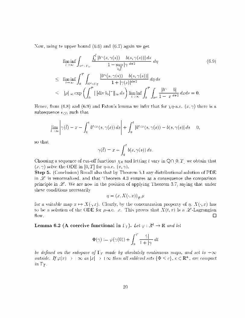
Now, using te upper bound (6.6) and (6.7) again we get

lim infi!1

ZRd��T

R �t

0jb�i(s; (s))� b(s; (s))j ds

1 + sup[0;�t]

j jd+2d� (6.9)

� lim infi!1

Z T

0

ZRd��T

jb�i(s; (s))� b(s; (s))j

1 + j (s)jd+2d� ds

� k�k1 exp

�Z T

0

k[div bs]�k1 ds

�lim infi!1

Z T

0

ZRd

jb�i � bj

1 + jxjd+2dxds = 0:

Hence, from (6.8) and (6.9) and Fatou's lemma we infer that for ��-a.e. (x; ) there is a

subsequence �i(l) such that

liml!1

����� (�t)� x�

Z �t

0

b�i(l)(s; (s)) ds

�����+Z �t

0

jb�i(l)(s; (s))� b(s; (s)j ds = 0;

so that

(�t) = x+

Z �t

0

b(s; (s)) ds:

Choosing a sequence of cut-o� functions �R and letting t vary in Q \ [0; T ] we obtain that

(x; ) solve the ODE in [0; T ] for �-a.e. (x; ).

Step 5. (Conclusion) Recall also that by Theorem 5.1 any distributional solution of PDE

in L is renormalized, and that Theorem 4.3 ensures as a consequence the comparison

principle in L . We are now in the position of applying Theorem 3.7, saying that under

these conditions necessarily

� = (x;X(�; x))# ��

for a suitable map x 7! X(�; x). Clearly, by the concentration property of �, X(�; x) has

to be a solution of the ODE for ��-a.e. x. This proves that X(t; x) is a L -Lagrangian

ow.

Lemma 6.2 (A coercive functional in �T ). Let ' : Rd ! R and let

�( ) := '( (0)) +

Z T

0

j _ j

1 + j jdt

be de�ned on the subspace of �T made by absolutely continuous maps, and set to +1

outside. If '(x)! +1 as jxj ! +1 then all sublevel sets f� � cg, c 2 R+ , are compact

in �T .

20

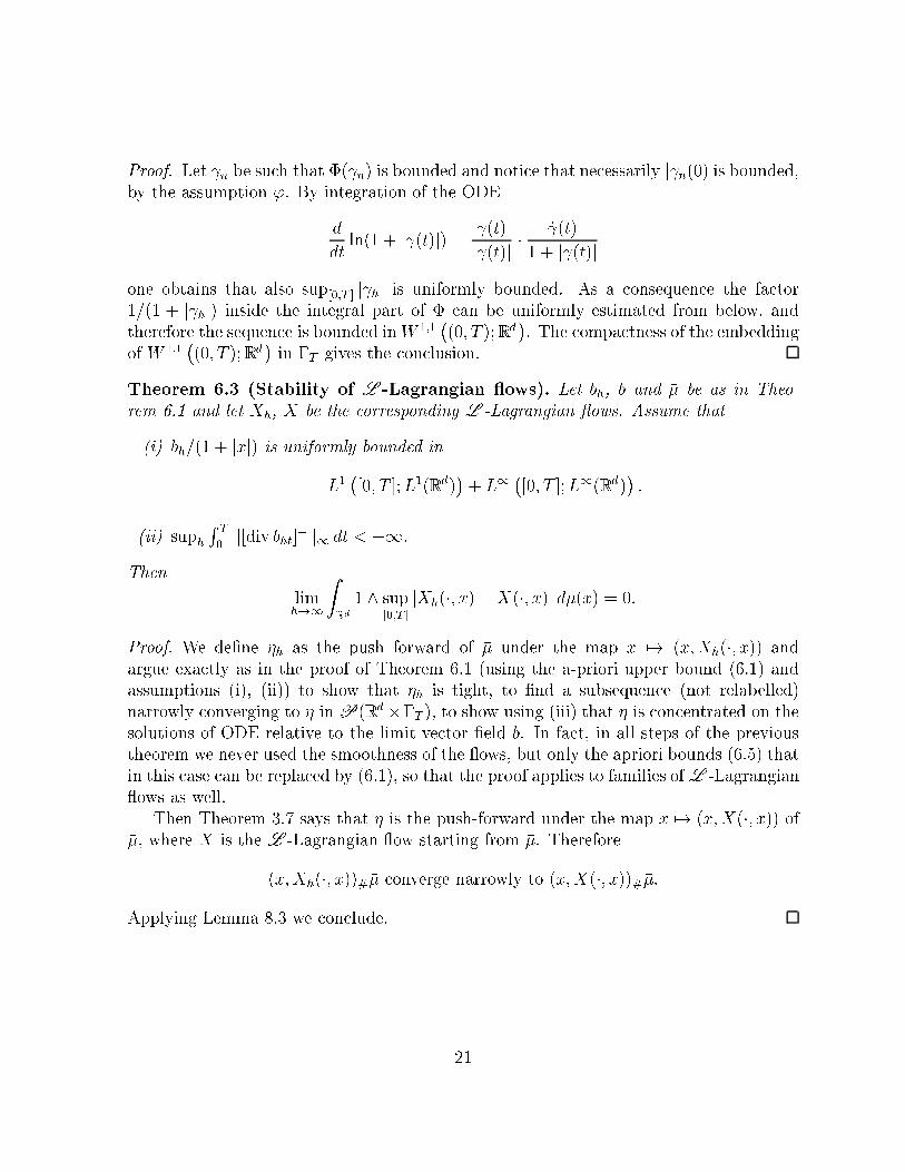
Proof. Let n be such that �( n) is bounded and notice that necessarily j n(0) is bounded,

by the assumption '. By integration of the ODE

d

dtln(1 + j (t)j) =

(t)

j (t)j�

_ (t)

1 + j (t)j

one obtains that also sup[0;T ] j hj is uniformly bounded. As a consequence the factor

1=(1 + j hj) inside the integral part of � can be uniformly estimated from below, and

therefore the sequence is bounded inW 1;1�(0; T );Rd

�. The compactness of the embedding

of W 1;1�(0; T );Rd

�in �T gives the conclusion.

Theorem 6.3 (Stability of L -Lagrangian ows). Let bh, b and �� be as in Theo-

rem 6.1 and let Xh, X be the corresponding L -Lagrangian ows. Assume that

(i) bh=(1 + jxj) is uniformly bounded in

L1�[0; T ];L1(Rd)

�+ L1

�[0; T ];L1(Rd)

�:

(ii) suphR T0k[div bht]

�k1 dt < +1.

Then

limh!1

ZRd

1 ^ sup[0;T ]

jXh(�; x)�X(�; x)j d��(x) = 0:

Proof. We de�ne �h as the push forward of �� under the map x 7! (x;Xh(�; x)) and

argue exactly as in the proof of Theorem 6.1 (using the a-priori upper bound (6.1) and

assumptions (i), (ii)) to show that �h is tight, to �nd a subsequence (not relabelled)

narrowly converging to � inP(Rd ��T ), to show using (iii) that � is concentrated on the

solutions of ODE relative to the limit vector �eld b. In fact, in all steps of the previous

theorem we never used the smoothness of the ows, but only the apriori bounds (6.5) that

in this case can be replaced by (6.1), so that the proof applies to families ofL -Lagrangian

ows as well.

Then Theorem 3.7 says that � is the push-forward under the map x 7! (x;X(�; x)) of

��, where X is the L -Lagrangian ow starting from ��. Therefore

(x;Xh(�; x))#�� converge narrowly to (x;X(�; x))#��.

Applying Lemma 8.3 we conclude.

21

7 An application to the Key�tz{Kranzer system of

conservation laws

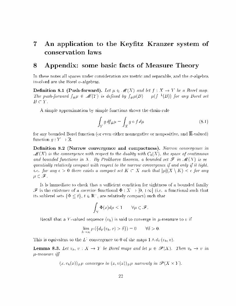
8 Appendix: some basic facts of Measure Theory

In these notes all spaces under consideration are metric and separable, and the �-algebra

involved are the Borel �-algebras.

De�nition 8.1 (Push-forward). Let � 2 M (X) and let f : X ! Y be a Borel map.

The push-forward f#� 2 M (Y ) is de�ned by f#�(B) = �(f�1(B)) for any Borel set

B � Y .

A simple approximation by simple functions shows the chain-ruleZY

g df#� =

ZX

g Æ f d� (8.1)

for any bounded Borel function (or even either nonnegative or nonpositive, and R -valued)

function g : Y ! R.

De�nition 8.2 (Narrow convergence and compactness). Narrow convergence in

M (X) is the convergence with respect to the duality with Cb(X), the space of continuous

and bounded functions in X. By Prokhorov theorem, a bounded set F in M (X) is se-

quentially relatively compact with respect to the narrow convergence if and only if it tight,

i.e. for any � > 0 there exists a compact set K � X such that j�j(X n K) < � for any

� 2 F .

It is immediate to check that a suÆcient condition for tightness of a bounded family

F is the existence of a coercive functional � : X ! [0;+1] (i.e. a functional such that

its sublevel sets f� � tg, t 2 R+ , are relatively compact) such thatZX

�(x)d� � 1 8� 2 F :

Recall that a Y -valued sequence (vh) is said to converge in �-measure to v if

limh!1

� (fdY (vh; v) > Æg) = 0 8Æ > 0:

This is equivalent to the L1 convergence to 0 of the maps 1 ^ dY (vh; v).

Lemma 8.3. Let vh; v : X ! Y be Borel maps and let � 2 P(X). Then vh ! v in

�-measure i�

(x; vh(x))#� converges to (x; v(x))#� narrowly in P(X � Y ).

22

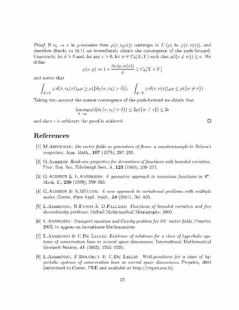
Proof. If vh ! v in �-measure then '(x; vh(x)) converges in L1(�) to '(x; v(x)), and

therefore thanks to (8.1) we immediately obtain the convergence of the push-forward.

Conversely, let Æ > 0 and, for any � > 0, let w 2 Cb(X;Y ) such that �(fv 6= wg) � �. We

de�ne

'(x; y) := 1 ^dY (y; w(x))

Æ2 Cb(X � Y )

and notice thatZX�Y

'd(x; vh(x))#� � �(fdY (w; vh) > Æg);

ZX�Y

'd(x; v(x))#� � �(fw 6= vg):

Taking into account the narrow convergence of the push-forward we obtain that

lim suph!1

�(fdY (v; vh) > Æg) � 2�(fw 6= vg) � 2�

and since � is arbitrary the proof is achieved.

References

[1] M.Aizenman: On vector �elds as generators of ows: a counterexample to Nelson's

conjecture. Ann. Math., 107 (1978), 287{296.

[2] G.Alberti: Rank-one properties for derivatives of functions with bounded variation.

Proc. Roy. Soc. Edinburgh Sect. A, 123 (1993), 239{274.

[3] G.Alberti & L.Ambrosio: A geometric approach to monotone functions in Rn .

Math. Z., 230 (1999), 259{316.

[4] G.Alberti & S.M�uller: A new approach to variational problems with multiple

scales. Comm. Pure Appl. Math., 54 (2001), 761{825.

[5] L.Ambrosio, N.Fusco & D.Pallara: Functions of bounded variation and free

discontinuity problems. Oxford Mathematical Monographs, 2000.

[6] L.Ambrosio: Transport equation and Cauchy problem for BV vector �elds. Preprint

2003, to appear on Inventiones Mathematicae.

[7] L.Ambrosio & C.De Lellis: Existence of solutions for a class of hyperbolic sys-

tems of conservation laws in several space dimensions. International Mathematical

Research Notices, 41 (2003), 2205{2220.

[8] L.Ambrosio, F.Bouchut & C.De Lellis: Well-posedness for a class of hy-

perbolic systems of conservation laws in several space dimensions. Preprint, 2003

(submitted to Comm. PDE and available at http://cvgmt.sns.it).

23

[9] L.Ambrosio, N.Gigli, G.Savar�e: Gradient ows in metric spaces and in the

Wasserstein space of probability measures. Book in preparation, to be published by

Birkh�auser.

[10] J.-D.Benamou & Y.Brenier: Weak solutions for the semigeostrophic equation

formulated as a couples Monge-Ampere transport problem. SIAM J. Appl. Math., 58

(1998), 1450{1461.

[11] F.Bouchut & F.James: One dimensional transport equation with discontinuous

coeÆcients. Nonlinear Analysis, 32 (1998), 891{933.

[12] F.Bouchut: Renormalized solutions to the Vlasov equation with coeÆcients of

bounded variation. Arch. Rational Mech. Anal., 157 (2001), 75{90.

[13] A.Bressan: An ill posed Cauchy problem for a hyperbolic system in two space di-

mensions. Preprint, 2003.

[14] I.Capuzzo Dolcetta & B.Perthame: On some analogy between di�erent ap-

proaches to �rst order PDE's with nonsmooth coeÆcients. Adv. Math. Sci Appl., 6

(1996), 689{703.

[15] A.Cellina: On uniqueness almost everywhere for monotonic di�erential inclusions.

Nonlinear Analysis, TMA, 25 (1995), 899{903.

[16] A.Cellina & M.Vornicescu: On gradient ows. Journal of Di�erential Equa-

tions, 145 (1998), 489{501.

[17] F.Colombini & N.Lerner: Uniqueness of continuous solutions for BV vector

�elds. Duke Math. J., 111 (2002), 357{384.

[18] F.Colombini & N.Lerner: Uniqueness of L1 solutions for a class of conormal

BV vector �elds. Preprint, 2003.

[19] F.Colombini & J.Rauch: Unicity and nonunicity for nonsmooth divergence free

transport. Preprint, 2003.

[20] M.Cullen & W.Gangbo: A variational approach for the 2-dimensional semi-

geostrophic shallow water equations. Arch. Rational Mech. Anal., 156 (2001), 241{

273.

[21] M.Cullen & M.Feldman: Lagrangian solutions of semigeostrophic equations in

physical space. To appear.

[22] C.Dafermos:

24

[23] N.De Pauw: Non unicit�e des solutions born�ees pour un champ de vecteurs BV en

dehors d'un hyperplan. C.R. Math. Sci. Acad. Paris, 337 (2003), 249{252.

[24] R.J. Di Perna & P.L.Lions: Ordinary di�erential equations, transport theory and

Sobolev spaces. Invent. Math., 98 (1989), 511{547.

[25] L.C.Evans & R.F.Gariepy: Lecture notes on measure theory and �ne properties

of functions, CRC Press, 1992.

[26] H.Federer: Geometric measure theory, Springer, 1969.

[27] M.Hauray: On Liouville transport equation with potential in BVloc. (2003) To ap-

pear on Comm. in PDE.

[28] M.Hauray: On two-dimensional Hamiltonian transport equations with Lploc coeÆ-

cients. (2003) To appear on Ann. Nonlinear Analysis IHP.

[29] P.L.Lions: Sur les �equations di��erentielles ordinaires et les �equations de transport.

C. R. Acad. Sci. Paris S�er. I, 326 (1998), 833{838.

[30] G.Petrova & B.Popov: Linear transport equation with discontinuous coeÆcients.

Comm. PDE, 24 (1999), 1849{1873.

[31] F.Poupaud & M.Rascle: Measure solutions to the liner multidimensional trans-

port equation with non-smooth coeÆcients. Comm. PDE, 22 (1997), 337{358.

[32] L.C.Young: Lectures on the calculus of variations and optimal control theory, Saun-

ders, 1969.

25