Oligopoly Competition in Fixed CostEnvironments

Yvonne DurhamWestern Washington University

Kevin McCabe, Mark A Olson,Stephen Rassenti and Vernon Smith

Interdisciplinary Center for Economic ScienceGeorge Mason University∗

September 18, 2003

Abstract

Many industries with avoidable fixed costs face competitive priceinstability problems in an attempt to maintain profitability. We de-signed an experimental environment where profitability is eroded bythe addition of sunk and avoidable fixed costs. While we cannot rejectthe hypothesis that sunk fixed costs have no effect on prices, we ob-serve a pattern of price signaling and responses which maintain abovenormal profits. This success implies that a firm does not have to exitsuch an industry in order to avoid loses, and may help to explain whysome competitive industries appear to maintain an inefficient numberof firms.

Keywords. Industrial Organization, Fixed Cost, Experimental Economics

JEL Classifications. L11, C92

∗We are grateful to the National Science Foundation, Grant no. IRI–8921141 for sup-port. We express our appreciation for the invaluable programming assistance of Zhu Li.

1

1 Introduction

Traditional economic theory tells a story about the ballistics of firm entryand exit in response to profits and losses normalized in relation to the marketopportunity costs of the firm, (see e.g. Smith (1974)). The research reportedin this paper began with the following question: in oligopolistic industries iffirms are making losses are there alternative strategies, besides exit or explicitprice collusion, that firms might pursue to avoid losses? In addressing thisquestion we were aware that the standard story is complicated by two distinctconcepts of fixed cost: traditional sunk costs and avoidable fixed cost. Hence,we wanted to include both sunk and avoidable fixed cost parameters in ourstudy of the dynamics of price competition1 in oligopoly behavior. In thisstudy, however, we do not independently vary the two kinds of fixed cost.Instead, holding constant the non-cooperative equilibrium, we vary the slopeof the linear demand, affording different potential rewards to firm attemptsto coordinate a price increase.

Many industries with substantial avoidable fixed costs face competitiveprice instability problems in an attempt to maintain normal profitability. Intransportation industries most of the direct cost is independent of the cargotransported, but can be avoided if the trip is canceled. For example, addingpassengers to an airline flight may increase cost somewhat, but most of thecost is for fuel and crew, and can be avoided by not flying. Similarly, electricpower generators incur an avoidable fixed cost just to maintain spinningreadiness to generate power. Large fixed costs often involve non-fungiblecapital, making exit a costly strategy so that firms avoid it and favor otherstrategies. For example, the airline industry has been very innovative indesigning fare structures that impose penalties on discounted tickets if theholder cancels or changes her flight plan leaving the airline with empty seatson the flight. Recently, some airlines are offering no-refund tickets and $100change fees. Such penalties enable the airline to recover some of their fixedflight costs. Yet in spite of these adaptive pricing policies, the industry hasbeen plagued by losses precipitated by the competition to fill seats.

Telser’s (1988) analysis and illustration of allocation problems createdby the existence of avoidable fixed costs, in which the core is empty, has

1We use the terms competition and competitive to refer to rivalry among the firmsparticipating in the market, this is a behavioral definition (see S. Martin (2003), for adiscussion of the term competition). We use the term competitive price to refer to theprice that clears the market.

2

inspired experimental market studies designed to investigate these demand-ing environments. Van Boening and Wilcox (1996) developed an avoid-able cost experimental design, in which the double auction institution—longknown for its capacity to produce efficient competitive outcomes in stressfulenvironments—does not converge to an efficient allocation. In their discretecost environment, any market tendency to converge to a uniform “competi-tive” price allows inefficient higher cost suppliers to displace an efficient lowercost firm. This is because an efficient firm with high avoidable fixed costsrequires a larger volume of sales than an inefficient firm to be profitable. Atthe competitive prices that would maintain this high volume, an inefficientsmaller firm can enter profitably and impose losses on the more efficient firm.

Durham et al. (1996) have proposed a computer assisted two-part pricingmechanism in which firms can charge a vendor’s fee in addition to postingunit prices and quantities as a potential means of overcoming the allocationproblems that arise in these avoidable fixed cost environments. The vendor’sfee, which must be paid by simulated fully revealing buyers before units canbe purchased, provides a means whereby avoidable costs can be covered be-fore units are committed for sale. (An alternative mechanism would allowfirms to specify a minimum as well as a maximum purchase volume.) Theposted-offer/vendor-fee experiments reported by Durham et al. (1996) yieldimproved but not ideal results. While the experiments achieve long sequencesof efficient allocations, those outcomes yielded to episodes of instability. Theresults converge to more efficient levels than in the double auction experi-ments reported by Van Boening and Wilcox. However, the two sets of experi-ments are not comparable in terms of experience and number of periods. TheDurham et al. experiments used much longer time sequences of repeat playthan those of Van Boening and Wilcox, and generally, more repeated playresults in more efficient outcomes in experimental double auction markets.

In a recent paper, Offerman and Potters (2002) examine the effect of entryfees on prices when two subjects are chosen from a group of four subjects toact as firms. They provide marginal evidence for an effect of a fixed entryfee (the fee is paid only once per five market periods). The potential forlosses was not discernible from the paper. In Buchheit and Feltovich (2000)subjects play a repeated two-person Bertrand-Edgeworth game, with demandand costs similar to Kruse et al.. Subjects incurred a sunk (unavoidable)cost. They find that sunk costs have a non-monotonic effect on prices, whichappear to decrease with time.

In this paper, the motivation parallels Van Boening and Wilcox, and

3

Durham et al., except that we compare a traditional variable cost environ-ment with one in which both sunk and avoidable fixed costs are added tothe variable costs. A traditional environment is designed to provide a welldefined (risk neutral) pure strategy equilibrium, which is profitable to each offive symmetric firms, while the profitability is eroded by the addition of sunkand avoidable fixed costs in the second environment. In fact, any tendencyto minimize losses by converging to the competitive-Nash price of the tradi-tional environment produces losses in the fixed cost environment. Because ofthe sunk fixed costs, these losses can only be partially reduced by producingnothing.

2 Environment

In each experimental session, five subjects are recruited, each to representone of five firms with identical cost structures. The subjects were under-graduates at the University of Arizona. The experiments were run in 1992and the average payoff was $20.25. Firms incur three kinds of costs in eachperiod: (1) sunk cost (called “unavoidable” fixed cost in the instructions),(2) avoidable fixed cost (called “starting” cost in the instructions), and (3)variable cost in discrete marginal form. Two different cost treatments arestudied. In the first treatment, categories (1) and (2) of fixed cost are eachzero. In the second, each firm has a sunk fixed cost of 150 and an avoidablefixed cost of 220. The marginal unit cost conditions are the same in bothtreatments: each firm can produce 100 units at a cost of 4 per unit, 100additional units at cost 4.5 per unit, and 100 at a cost of 5 per unit. Twodifferent demand treatments are studied: demand Le, p = 17 − 0.01q, anddemand He, p = 11.6−0.0055q, where (p, q) = (price, quantity). Demand Le

has a lower (steeper demand curve) price elasticity than demand He at theequilibrium price (which is the same for both demand curves). The two de-mand curves provide a comparison between one environment (Demand Le)where it is easier to raise prices without a large loss in quantity sold andanother environment (Demand He) where prices can be raised only with alarge loss in quantity sold.

Simulated buyers are programmed to reveal demand. Units are chosenat random, without replacement, from the aggregate demand and allocatedto 114 buyers consisting of 100 small buyers and 14 large buyers. The largebuyer has five times as many units as a small buyer. In demand condition

4

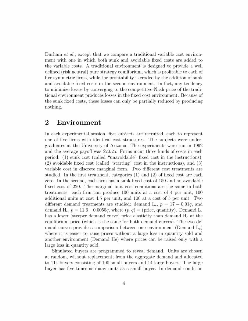
Inelastic Demand Elastic DemandOnce Twice Once Twice

Experienced Experienced Experienced ExperiencedSeller $13.50 $0 $13.50 $0Cost Endowment Endowment Endowment EndowmentNo Fixed 5(60) 4(80) 4(60) 4(50)Fixed 4(60) 3(80) 3(60) 3(80)Total 9 7 7 7

Table 1: The number of sessions and trading periods (in parenthesis) persession by treatment condition. The total number of sessions is 30.

Le small buyers demand a maximum of 10 units (i.e. at a zero price) andlarge buyers demand a maximum of 50 units.2 In demand condition He smallbuyers demand a maximum of 12 units and large buyers demand a maximumof 60 units.

The environment was sufficiently complex that we trained subjects in tenperiod experiments. We then brought them back in groups that were once-experienced to participate in experiments that were run for 60 periods. Thesetwice-experienced subjects were then asked to return for a third time to par-ticipate in a set of 80 period experiments (except for the twice-experienced,no sunk cost, elastic demand sessions, which had 50 periods per session3).The cost parameters remained unchanged for all levels of experience, butsubject groups were not constrained to remain of identical composition forall experience levels. Because the likelihood of losses was high, especially forthe trainers (the first ten period sessions), subjects received initial endow-ments of $5.00 working capital in the trainer, $13.50 in the once-experiencedsessions, but no endowment in the twice-experienced sessions.

The two levels of subject experience, two demand levels, and two costtreatments forms a 2× 2× 2 design. Table 1 summarizes the parameters of

2The software makes provision for markets in which human buyers can be added, andthe matching of buyers and firms can be assisted by a smart market center which maximizessurplus. Although Durham et al. (1996) makes use of the smart market features, theprovision for human buyers has not yet been implemented in the software. When it is,one could run experiments with, say, 5 human buyers and 100 simulated small buyers.

3The number of periods was reduced to alleviate the boredom for 80 identical periods.The statistical analysis accounts for the different number of periods.

5

the environment and lists the number of experiments (and number of tradingperiods) for each of the 8 treatment cells. The periods in the once-experiencedsubject groups lasted 75 seconds, and the periods in the twice-experiencedsubject groups lasted 45 seconds. We reduced the length of the periods inthe twice-experienced groups because in the earlier experiments there wassubstantial “dead” time between the last offer and the end of the period.

3 Institution

At the beginning of each trading period, each firm independently choosesa price and quantity (pi, qi). Simulated buyers are chosen in random orderwithout replacement and each buyer purchases all units demanded at thelowest price quoted among the active firms in the current state of the market.If that firm’s supply is inadequate to satisfy the buyer’s demand, the buyerpurchases from the remaining firm with the lowest price. If two or morefirms quote tied prices, the buyer is randomly allocated to one of these firms.These procedures are identical to the computerized, posted offer market (seeKetcham, Smith, Williams (1984)). We now discuss the procedures thatdiffer from this standard market.

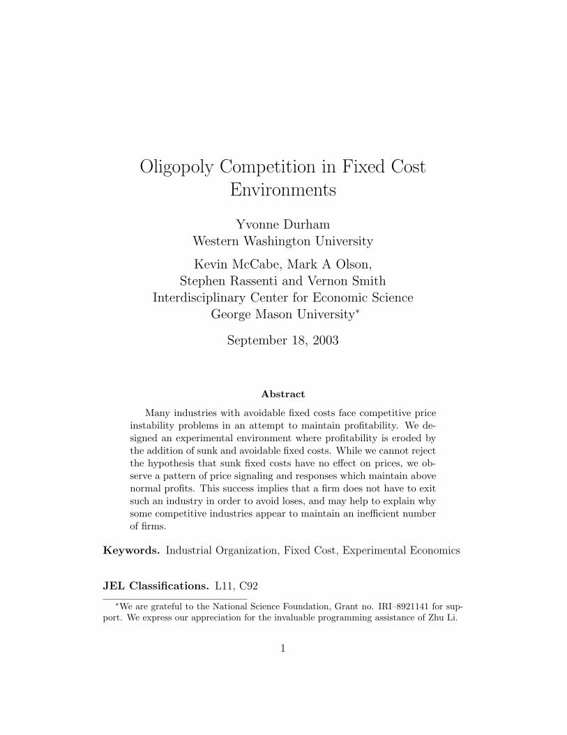
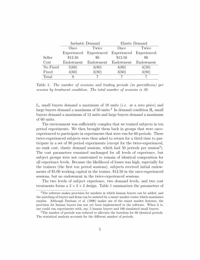
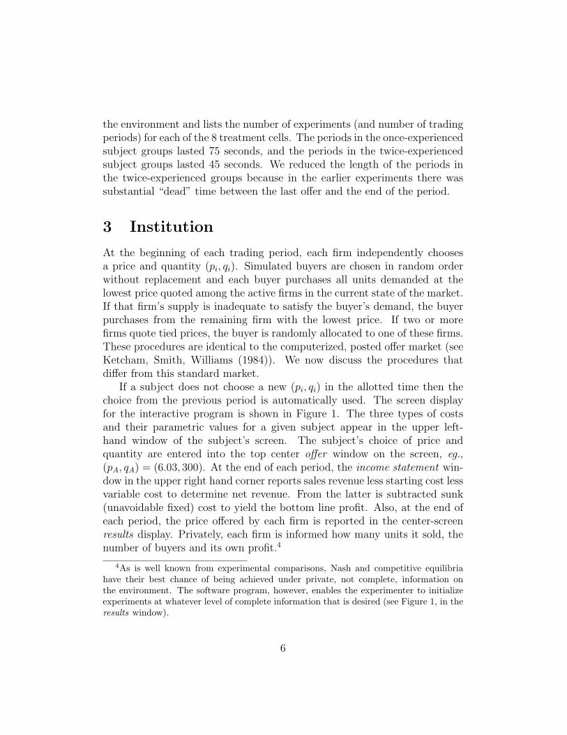
If a subject does not choose a new (pi, qi) in the allotted time then thechoice from the previous period is automatically used. The screen displayfor the interactive program is shown in Figure 1. The three types of costsand their parametric values for a given subject appear in the upper left-hand window of the subject’s screen. The subject’s choice of price andquantity are entered into the top center offer window on the screen, eg.,(pA, qA) = (6.03, 300). At the end of each period, the income statement win-dow in the upper right hand corner reports sales revenue less starting cost lessvariable cost to determine net revenue. From the latter is subtracted sunk(unavoidable fixed) cost to yield the bottom line profit. Also, at the end ofeach period, the price offered by each firm is reported in the center-screenresults display. Privately, each firm is informed how many units it sold, thenumber of buyers and its own profit.4

4As is well known from experimental comparisons, Nash and competitive equilibriahave their best chance of being achieved under private, not complete, information onthe environment. The software program, however, enables the experimenter to initializeexperiments at whatever level of complete information that is desired (see Figure 1, in theresults window).

6

��������������� �������������������������� ������������������������������������������������� ���������� ��������������� !�����!�"#������ $&%�'�(*)�+-,�.0/ � +�1�24365�5�7 $�$ $�$ $$ � 2�(�892-,*'�: � +�1�243<;=�7 $�$ $�$>1�(�?!@�1A8@�)�@9'9B�@ ;�C�7�7 $$ $�$ $�$>1�2�(�892-,*'�:ED9+�1�2EF ;=�7 $$HG (�8�,!(JI ?!@ � +�1�243 $�$ � B�K�I�@�8L+�M#%�'�,!2�1N3PO�7�7 $�$Q)�(�8�,!(JI ?!@ED9+�1�2EF ;O�=�7 $$ %�'�,!2�1 � +�1�2SR�@�8�%�'�,!2T$�$ $�$UF�F�F�F�F�F�F�F�F�F�F�F�F�F�F�F�F�F�F�F�F�F�F�F�FV$$ ;!F-;�7�7 WN/X7�7 $�$ %�'�,!2EY98�,D@03[Z\/X7O $�$ '�@�2]8@�)�@9'9B�@ O�7�7 $$^;�7�;!F95�7�7 WN/_=�7 $�$ $�$`B�'�(*)�+-,�.0/ � +�1�2EF 5�5�7 $$a5�7�;!F�O�7�7 =b/X7�7 $�$ �c @]+�M�M*@�8E,�1AD9+'"M9,8�K"@�.0/�$�$ Y989+�M9,!2 C�7 $d ����������������������������������������������e d ��������������������������������������������������e d ��������������������������������������������������e

�*��f�f����� Y!@�8�,!+9.03 O � (JR�,!2�(�?g3 ;�Z7 � ?+�D�hb3PO5� Y!@�8�,!+9. 5 � @�1�B�?2�1 ������������������������i�������������� �j������������� kl���������������������� $ $$ Y � �J���������������k $ Z\/X7�7 Z\/X;�7 Z\/X7�; Z\/X7�C Z\/X7= $$ % �\�*���������������k $ O�7�7 $$ % �\�*����m�nf�k $ O�7�7 $$ � % ��i��������oi %�p ����� $ 5nq $$ Y ��� �X��k Y �*�����* $ C�7 $d Y98@�) ,!+!Bn1N3rY!: k ' � @s-243rY!:!%R ������������������������������������������������������������������������������e

������������������������������������������������������������������������������������������������������������������������������������������������������������ $ $d ����������������������������������������������������������������������������������������������������������������������������������������������������������eD c ('�:�@�I"+!sV3ut�v ,*'-D�8@�(�1*@03�wav .�@�D�8@�(�1*@03�xav 1zy ,!2�D c Rn89+�M9,!2�{�Rn8�,D@03ut�v k @�M�(!B�?2

��� %�'�,!2�1 �������� ����� Y98�,D@ ������ ����� Y989+�M9,!2 ���� d ����� O�7�7 ��������e d ��� Z\/X7�7 ������e d ��� C�7 ����e

Figure 1: Interactive Screen Display.

These results can be scrolled using the page down or page up keys toaccess perfect recall of the market’s past history. Immediately above theresults window appears a statement of the subject’s capital or cumulativecurrent balance: initial capital plus all profits minus all losses through thecurrent period. During a period the remaining time appears adjacent toclock, which is immediately above and to the right of the results window.

At the bottom of the screen is a calculator tool designed to assist a subjectin making an offer. By pressing a default key, the previous period’s quantity,price and profit appear in the space shown. By scrolling any two of the threevariables—quantity, price, and profit—the third is computed for the subjecton the assumption that all units are sold at the indicated price. For example,if units and profit are chosen, the calculator determines what selling pricewould generate the designated profit target. For the assumption to be validthat all units offered will be sold requires the subject to estimate residualdemand at the specified price, but the tool allows the outcome space to beeasily explored. During the experiment, subjects soon discover that all unitsoffered may not be sold.

7

4 Equilibrium and Predictions

When there are no fixed costs both demand conditions define a risk neutralBertrand–Nash pure strategy equilibrium at (pN

i , qNi ) = (5.0, 300) for each

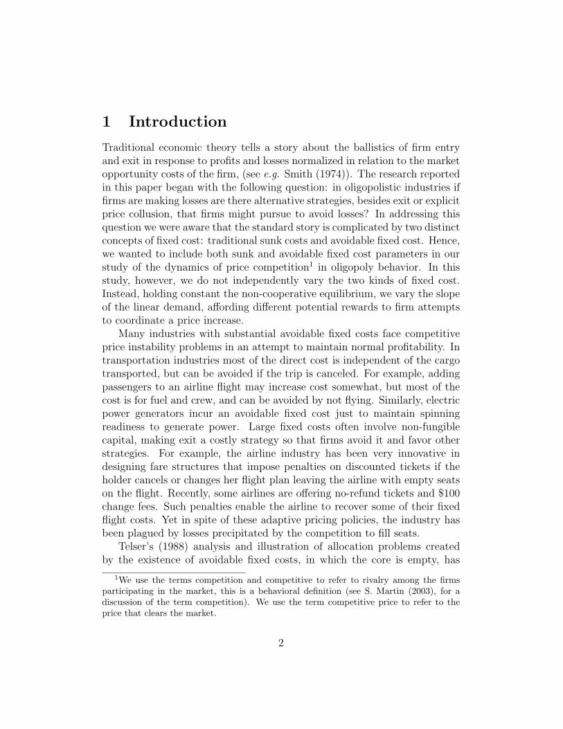
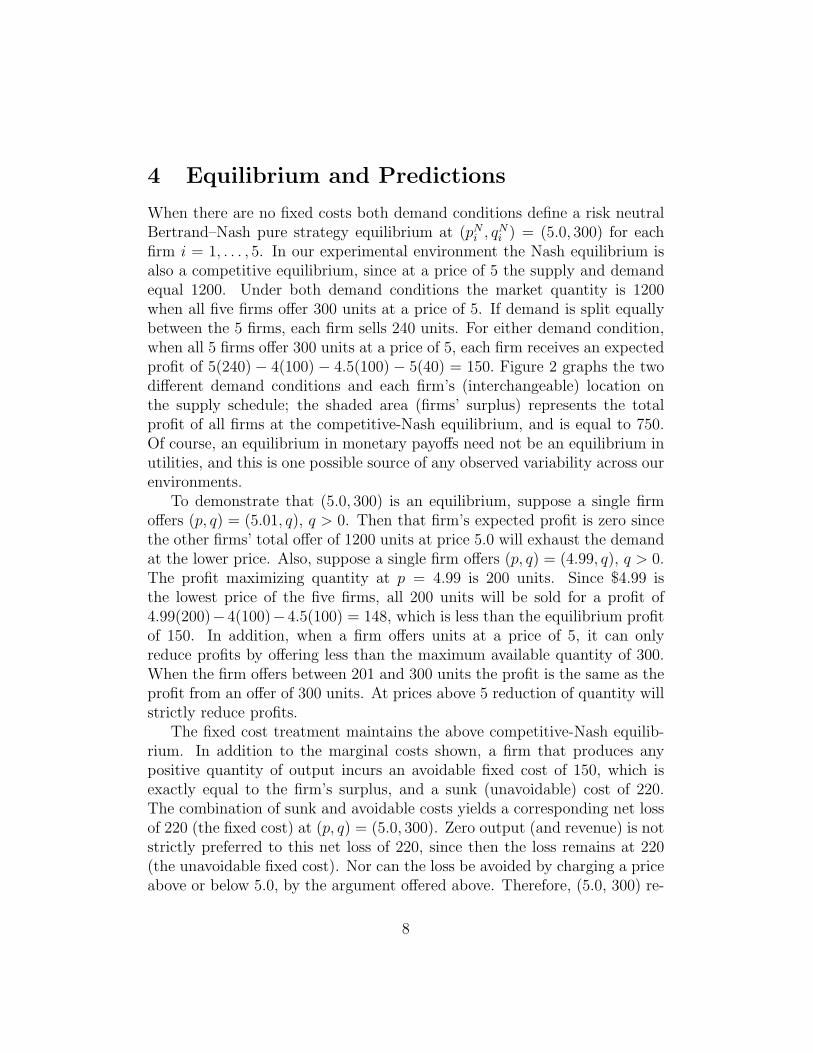
firm i = 1, . . . , 5. In our experimental environment the Nash equilibrium isalso a competitive equilibrium, since at a price of 5 the supply and demandequal 1200. Under both demand conditions the market quantity is 1200when all five firms offer 300 units at a price of 5. If demand is split equallybetween the 5 firms, each firm sells 240 units. For either demand condition,when all 5 firms offer 300 units at a price of 5, each firm receives an expectedprofit of 5(240)− 4(100) − 4.5(100) − 5(40) = 150. Figure 2 graphs the twodifferent demand conditions and each firm’s (interchangeable) location onthe supply schedule; the shaded area (firms’ surplus) represents the totalprofit of all firms at the competitive-Nash equilibrium, and is equal to 750.Of course, an equilibrium in monetary payoffs need not be an equilibrium inutilities, and this is one possible source of any observed variability across ourenvironments.

To demonstrate that (5.0, 300) is an equilibrium, suppose a single firmoffers (p, q) = (5.01, q), q > 0. Then that firm’s expected profit is zero sincethe other firms’ total offer of 1200 units at price 5.0 will exhaust the demandat the lower price. Also, suppose a single firm offers (p, q) = (4.99, q), q > 0.The profit maximizing quantity at p = 4.99 is 200 units. Since $4.99 isthe lowest price of the five firms, all 200 units will be sold for a profit of4.99(200)−4(100)−4.5(100) = 148, which is less than the equilibrium profitof 150. In addition, when a firm offers units at a price of 5, it can onlyreduce profits by offering less than the maximum available quantity of 300.When the firm offers between 201 and 300 units the profit is the same as theprofit from an offer of 300 units. At prices above 5 reduction of quantity willstrictly reduce profits.

The fixed cost treatment maintains the above competitive-Nash equilib-rium. In addition to the marginal costs shown, a firm that produces anypositive quantity of output incurs an avoidable fixed cost of 150, which isexactly equal to the firm’s surplus, and a sunk (unavoidable) cost of 220.The combination of sunk and avoidable costs yields a corresponding net lossof 220 (the fixed cost) at (p, q) = (5.0, 300). Zero output (and revenue) is notstrictly preferred to this net loss of 220, since then the loss remains at 220(the unavoidable fixed cost). Nor can the loss be avoided by charging a priceabove or below 5.0, by the argument offered above. Therefore, (5.0, 300) re-

8

Figure 2: Demand Figures.

9

mains a pure competitive-Nash equilibrium in the second environment. Thistheoretical results provides our first research question:

• Will mean contract prices be close to the risk neutral competitive-Nashprice of 5.0? (Statistical Hypothesis H0.)

But what will competing firms do in this harsh fixed cost environment?One solution would require withholding supply on the part of firms so thatno subset of the other firms could satisfy demand. Any such implicit contractto limit output by more than 20% would create residual demand conditionswhere a profitable mixed strategy Nash equilibrium with a distribution sup-port from somewhere above the Ramsey break–even price to the monopolyprice would rule. But even if this withholding agreement were enforced,earlier work which examined mixed strategy behavior in a zero fixed costoligopoly environment, found behavior which does not correspond to randompricing (Kruse, Rassenti, Reynolds and Smith, 1993).5 Instead of withhold-ing supply, a more obvious and easily implementable coordinating strategyfor the firms is to engage in price signaling, which we define empirically inthe next section. Although there is an incentive to signal in an attempt toachieve greater profits in both of the cost environments, in the fixed costenvironment no positive profit is possible without it.

By setting a higher price in this period a firm hopes that other firms willraise their prices next period. Why don’t firms see this as a ruse by thesignaling firm? A useful benchmark, at which signaling begins to becomea less costly strategy, is the Ramsey break–even price. Below the Ramseyprice losses are incurred, and since the firm is already incurring losses, thealternative is to raise its price. This unilateral action will produce zero sales,and one avoids all but the sunk cost. By offering yet a higher price a firmmay be strategically committing to a higher price in the next period, perhaps

5In that work there were four firms with identical constant marginal costs and residualdemand when three of the four priced competitively. The mixed strategy Nash equilibriumwas computed for different capacity levels by numerically solving the integral–differentialequations which describe the equilibrium conditions. These theoretical distributions pre-dict the qualitative direction of shift of the data with shifts in the capacity parameters.But the observed price distributions, (1) differed significantly from the predicted distribu-tions, and (2) exhibited too much auto correlation in time to be consistent with the Nashmixed strategy hypothesis. However there was a significant amount of continuing pricevariability over time that would not have been inconsistent with the signaling and cyclinghypotheses being examined here.

10

lower than its current price, but greater than its price in the previous period.Other firms are in the same position, and have a powerful incentive to followany such leader.

We further encourage the incentive for dynamic profit taking by reducingeach firm’s initial working capital across experience levels: (1) the trainerfirms who participated in only 10 trading periods are endowed with $5 eachper experiment; (2) once-experienced firms each received $13.50; and (3)twice-experienced firms receive no endowments. Consequently, for the lattersessions no net earnings are possible unless prices are maintained above theRamsey price when fixed costs are present. Since the subjects return forthree sessions, they are well aware of what has to be achieved if they are tomake a profit. We note here that we will use the term “Twice-experienced”to denote the environment where subjects were twice-experienced, receivedno endowments, and had either more or fewer periods than than the “Once-experienced” subject sessions. Any statistical test of experience level is notstrictly a test of experience, because of the confounding effects of endowmentand period numbers. But it is strictly a test between the two environments.We could have eliminated the “Once-experienced” sessions from our results,but we thought the observations were “interesting”.

The above considerations lead to the following research questions:

• Will Twice-experienced subjects adapt by maintaining higher meancontract prices than once-experienced subjects? (This will lead to sta-tistical hypothesis H1.)

• Will contract prices be higher in the fixed plus variable cost environ-ment than in the variable cost only environment? (Statistical Hypoth-esis H2.)

The range over which all firms can benefit by charging prices above thebreak even Ramsey price differ under the two different demand environments.Under the demand Le conditions, any given increase in price causes a smallerreduction in sales than under demand He. Consequently:

• Will mean contract prices will be higher under demand Le than underdemand He? (Statistical Hypothesis H3.)

We note, however, that the pure strategy Nash equilibrium and the com-petitive price equilibrium, both with and without fixed costs, are unaffected

11

by the change in demand structure. Thus, static Nash theory would predictno change in behavior in the demand Le and demand He environments.

Next, we consider the role of price signaling in these dynamic price-settingprocesses.6 We define a signal as occurring when offers are submitted whichare unlikely to be competitive in a world where price competition continues.Suppose that more quantity is submitted in a given period than can be soldat the posted prices. Then in the subsequent period, a price signal is definedas any price submitted by any firm that is greater than or equal to the lowestposted price that failed to attract buyers in the previous period. When allquantity submitted is sold at the posted prices in a given period (this can onlyhappen if some firms withhold capacity), then in the subsequent period, anyprice submitted by any firm that is greater than the highest price at whichall other firms could have sold if that firm had not competed, is considereda signal. The experiments reported are replete with such signals that weattribute to conscious efforts to induce price increases.

The next two questions simply mimic the first three with respect to theamount of signaling we should expect to observe if indeed there is a correla-tion between signaling and contract prices:

• Will twice-experienced subjects signal more frequently than once expe-rienced subjects? (Statistical Hypothesis H4.)

• Will more signals will be sent in the fixed cost environment than in theno fixed cost environment? (Statistical Hypothesis H5.)

When demand elasticity increases there is less room for price manipula-tion, so the profitability of a signal becomes much more tenuous as higherprices are less viable. This motivates our last question:

• Will more signals will be observed under demand He than under de-mand Le? (Statistical Hypothesis H6.)

5 Results

To examine the first set of questions, we must first provide a measure ofcontract price in an experimental period. We define the contract price in

6See Friedman and Hoggatt (1980, pp. 124–129, 147–154, 192–193) for a study ofexperimental oligopoly in which price signaling phenomena are analyzed, apparently forthe first time in the experimental literature.

12

Inelastic Demand Elastic DemandOnce Twice Once Twice

Experienced Experienced Experienced ExperiencedSeller $13.50 $0 $13.50 $0Cost Endowment Endowment Endowment EndowmentFixed 7.02 7.13 6.50 7.33CostNo Fixed 6.27 8.12 5.81 6.37Cost

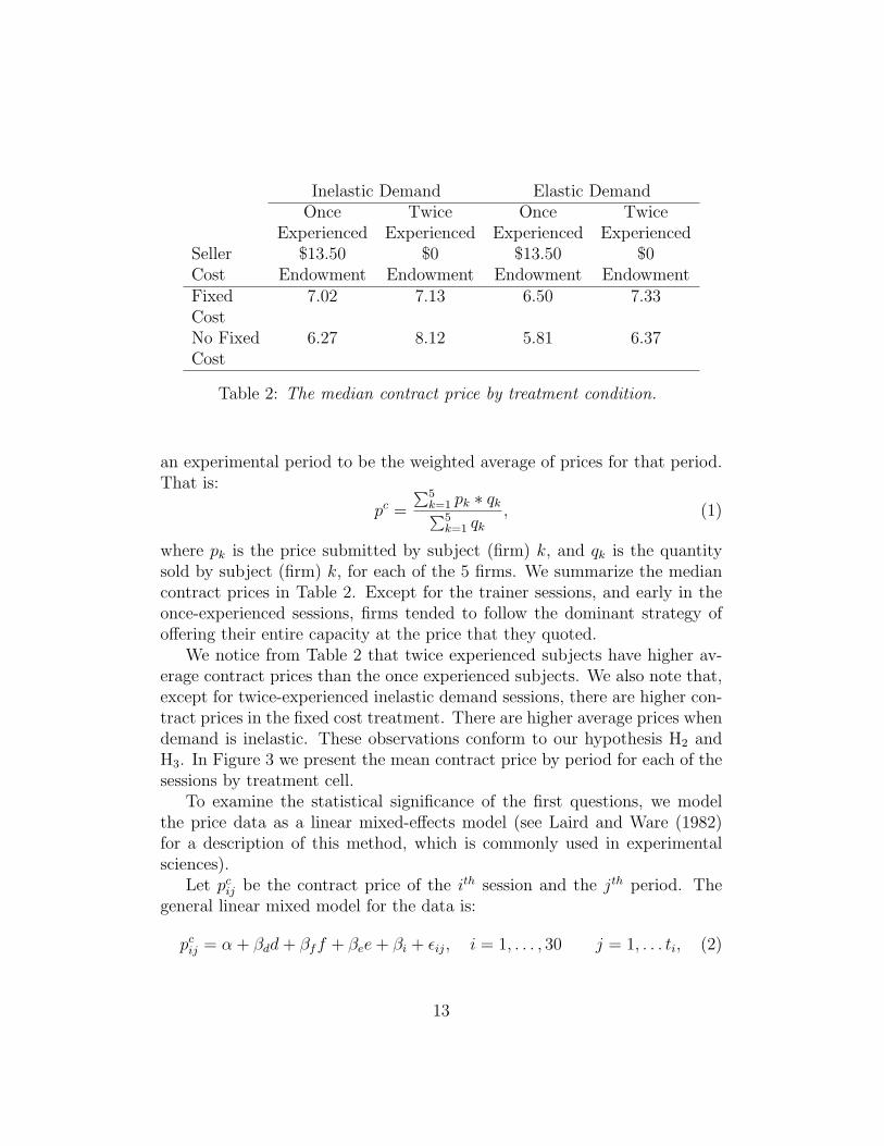
Table 2: The median contract price by treatment condition.

an experimental period to be the weighted average of prices for that period.That is:

pc =

∑5k=1 pk ∗ qk∑5

k=1 qk

, (1)

where pk is the price submitted by subject (firm) k, and qk is the quantitysold by subject (firm) k, for each of the 5 firms. We summarize the mediancontract prices in Table 2. Except for the trainer sessions, and early in theonce-experienced sessions, firms tended to follow the dominant strategy ofoffering their entire capacity at the price that they quoted.

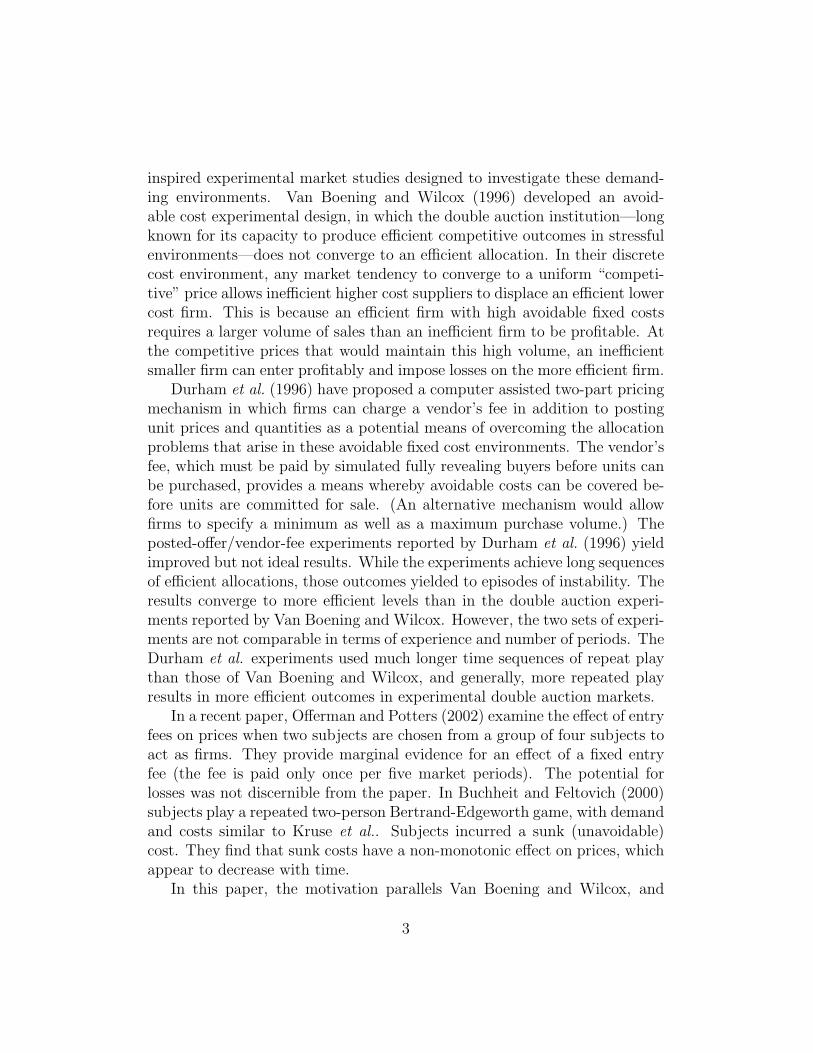
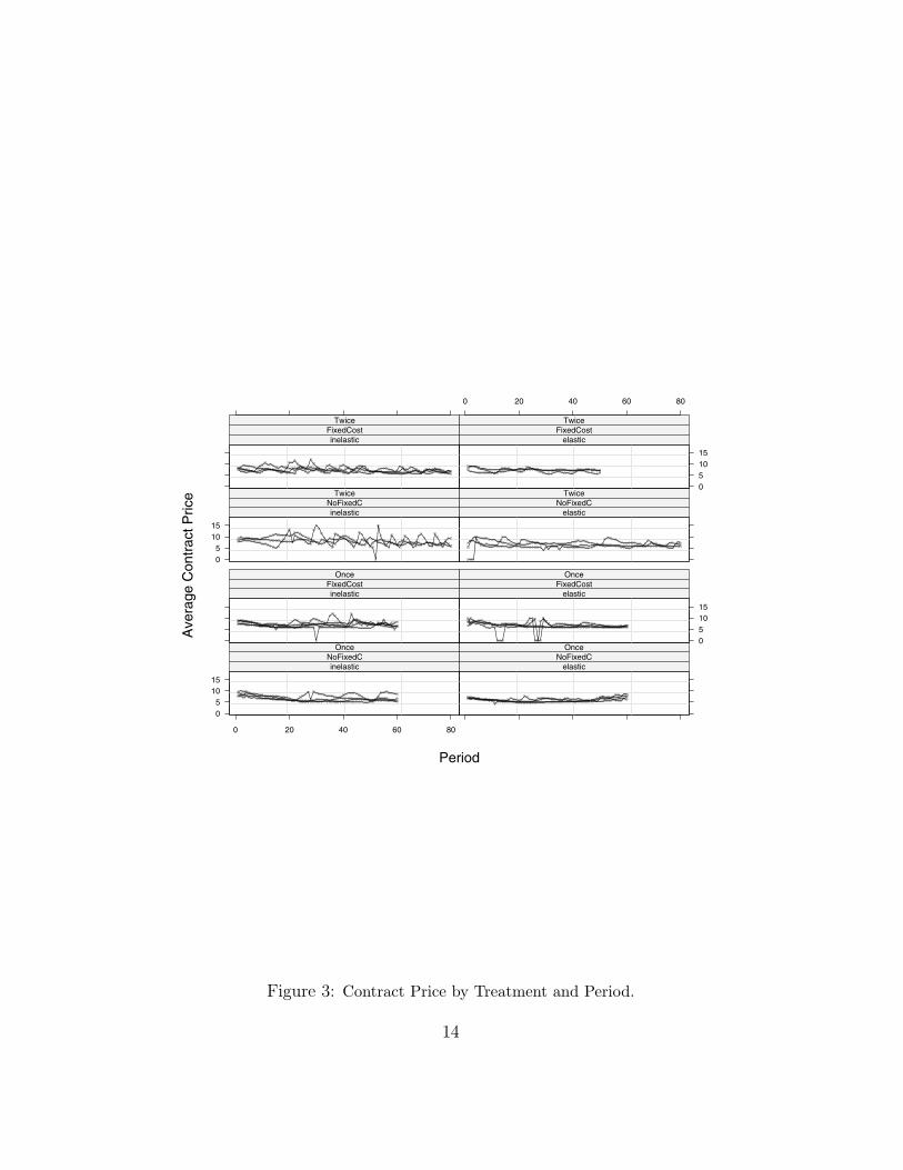
We notice from Table 2 that twice experienced subjects have higher av-erage contract prices than the once experienced subjects. We also note that,except for twice-experienced inelastic demand sessions, there are higher con-tract prices in the fixed cost treatment. There are higher average prices whendemand is inelastic. These observations conform to our hypothesis H2 andH3. In Figure 3 we present the mean contract price by period for each of thesessions by treatment cell.

To examine the statistical significance of the first questions, we modelthe price data as a linear mixed-effects model (see Laird and Ware (1982)for a description of this method, which is commonly used in experimentalsciences).

Let pcij be the contract price of the ith session and the jth period. The

general linear mixed model for the data is:

pcij = α + βdd + βff + βee + βi + εij, i = 1, . . . , 30 j = 1, . . . ti, (2)

13

05

1015

0 20 40 60 80

inelasticNoFixedC

Once

elasticNoFixedC

Once

inelasticFixedCost

Once

051015

elasticFixedCost

Once

05

1015

inelasticNoFixedC

Twice

elasticNoFixedC

Twice

inelasticFixedCost

Twice

051015

0 20 40 60 80

elasticFixedCost

Twice

Period

Ave

rage

Con

trac

t Pric

e

Figure 3: Contract Price by Treatment and Period.

14

Value Std.Error DF t-value p-valueIntercept 6.97 0.105 1938 66.40 < .0001

d -0.36 0.105 22 -3.49 0.0020f 0.10 0.105 22 0.98 0.3348e 0.33 0.105 22 3.19 0.0042

d:f 0.23 0.105 22 2.26 0.0337d:e -0.07 0.105 22 -0.72 0.4767f:e -0.15 0.105 22 -1.49 0.1479

d:f:e 0.18 0.105 22 1.76 0.0912

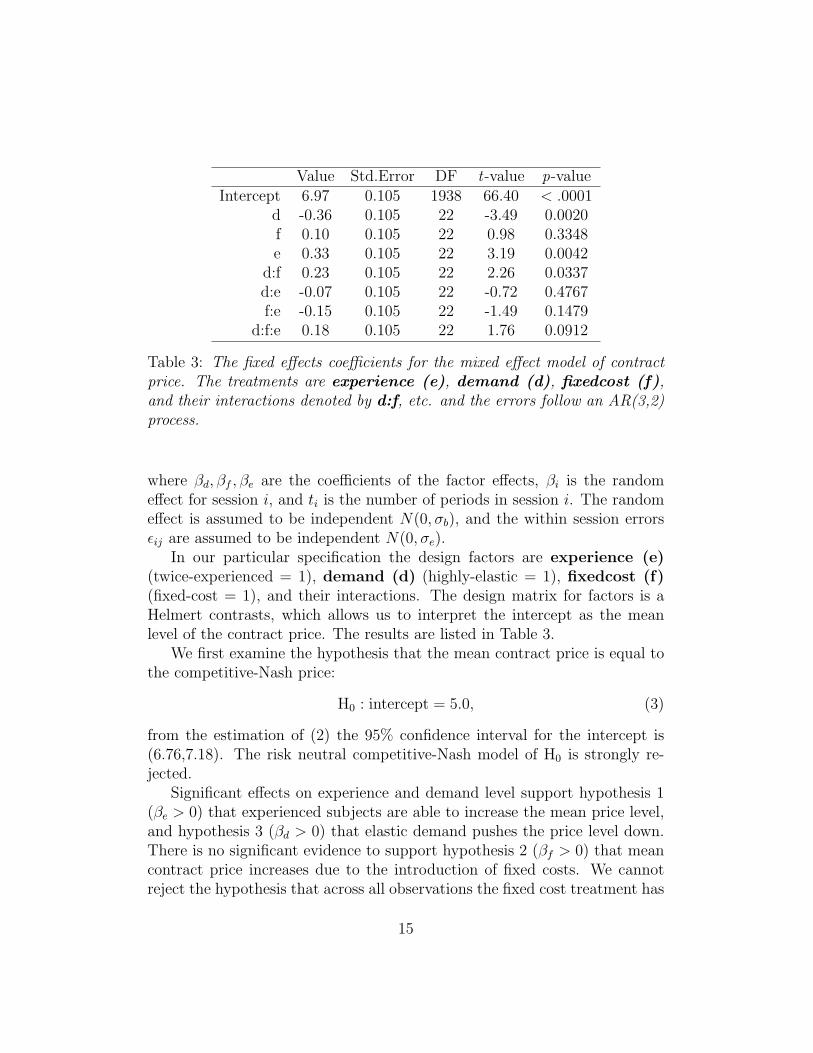
Table 3: The fixed effects coefficients for the mixed effect model of contractprice. The treatments are experience (e), demand (d), fixedcost (f),and their interactions denoted by d:f, etc. and the errors follow an AR(3,2)process.

where βd, βf , βe are the coefficients of the factor effects, βi is the randomeffect for session i, and ti is the number of periods in session i. The randomeffect is assumed to be independent N(0, σb), and the within session errorsεij are assumed to be independent N(0, σe).

In our particular specification the design factors are experience (e)(twice-experienced = 1), demand (d) (highly-elastic = 1), fixedcost (f)(fixed-cost = 1), and their interactions. The design matrix for factors is aHelmert contrasts, which allows us to interpret the intercept as the meanlevel of the contract price. The results are listed in Table 3.

We first examine the hypothesis that the mean contract price is equal tothe competitive-Nash price:

H0 : intercept = 5.0, (3)

from the estimation of (2) the 95% confidence interval for the intercept is(6.76,7.18). The risk neutral competitive-Nash model of H0 is strongly re-jected.

Significant effects on experience and demand level support hypothesis 1(βe > 0) that experienced subjects are able to increase the mean price level,and hypothesis 3 (βd > 0) that elastic demand pushes the price level down.There is no significant evidence to support hypothesis 2 (βf > 0) that meancontract price increases due to the introduction of fixed costs. We cannotreject the hypothesis that across all observations the fixed cost treatment has

15

Value Std.Error t-value p-valueIntercept 0.63 0.053 11.82 0.000

d 0.11 0.053 2.19 0.038f 0.14 0.053 2.66 0.014e 0.05 0.053 1.10 0.281

d:f 0.11 0.053 2.15 0.042d:e -0.03 0.053 -0.64 0.524f:e -0.08 0.053 -1.63 0.116

d:f:e 0.00 0.053 0.06 0.950

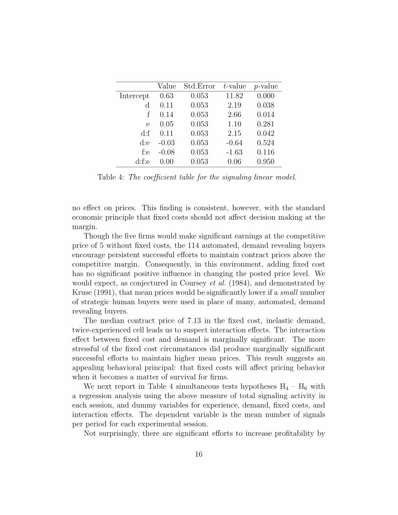
Table 4: The coefficient table for the signaling linear model.

no effect on prices. This finding is consistent, however, with the standardeconomic principle that fixed costs should not affect decision making at themargin.

Though the five firms would make significant earnings at the competitiveprice of 5 without fixed costs, the 114 automated, demand revealing buyersencourage persistent successful efforts to maintain contract prices above thecompetitive margin. Consequently, in this environment, adding fixed costhas no significant positive influence in changing the posted price level. Wewould expect, as conjectured in Coursey et al. (1984), and demonstrated byKruse (1991), that mean prices would be significantly lower if a small numberof strategic human buyers were used in place of many, automated, demandrevealing buyers.

The median contract price of 7.13 in the fixed cost, inelastic demand,twice-experienced cell leads us to suspect interaction effects. The interactioneffect between fixed cost and demand is marginally significant. The morestressful of the fixed cost circumstances did produce marginally significantsuccessful efforts to maintain higher mean prices. This result suggests anappealing behavioral principal: that fixed costs will affect pricing behaviorwhen it becomes a matter of survival for firms.

We next report in Table 4 simultaneous tests hypotheses H4 – H6 witha regression analysis using the above measure of total signaling activity ineach session, and dummy variables for experience, demand, fixed costs, andinteraction effects. The dependent variable is the mean number of signalsper period for each experimental session.

Not surprisingly, there are significant efforts to increase profitability by

16

increasing the number of price signals under the more stressful circumstances(elastic demand and fixed costs). But experience seems to have little to dowith the number of signals generated, though we have already observed thatit does significantly affect prices. How do experienced firms achieve higherprices? One intuitive explanation is that the subjects use price signals toprecommit to a higher pricing strategy. Or, as noted by a referee: “Perhapsit is the case that the experienced players read the same signals more in-sightfully, and thus more signals are not useful at the margin.” This led usto some ex post data mining.

For each individual experimental session, we estimated the influence ofthe presence of a signal on the mean contract price of the next period. Thus:

pcij = αi+βip

ci(j−1)+σiI(signali(j−1))+εij, j = 1, . . . , ti, i = 1, . . . , 30, (4)

where pcij is the contract price in period j of experimental session i, I(signalij))

is 1 if there is a signal in period j, session i and 0 if there is no signal, ti isthe number of periods in session i, and εij is the error term. Fourteen of thesessions had significant values for σi at the 5% level or better. However, thesignal measure was much more likely to have an effect in the twice experi-enced, inelastic demand sessions, which had 7 out of 7 significant values forσi at the 5% level, indicating that this signal measure was likely to have hadan effect on subsequent contract prices.

On an individual level we look at the commitment of subjects to maintaina high price after sending a price signal. Thus:

pij = βipi(j−2) + σiI(signali(j−1)) + εij, j = 1, . . . , ti, i = 1, . . . , 150, (5)

where pij is the offer price in period j by subject i, I(signalij)) is 1 if thereis a signal in period j, by subject i and 0 if there is no signal, and εij is theerror term. Seventy-eight percent of the subjects had positive values for σi,indicating that when a signal was sent the subject was more likely to submita price higher than the price in the previous period.

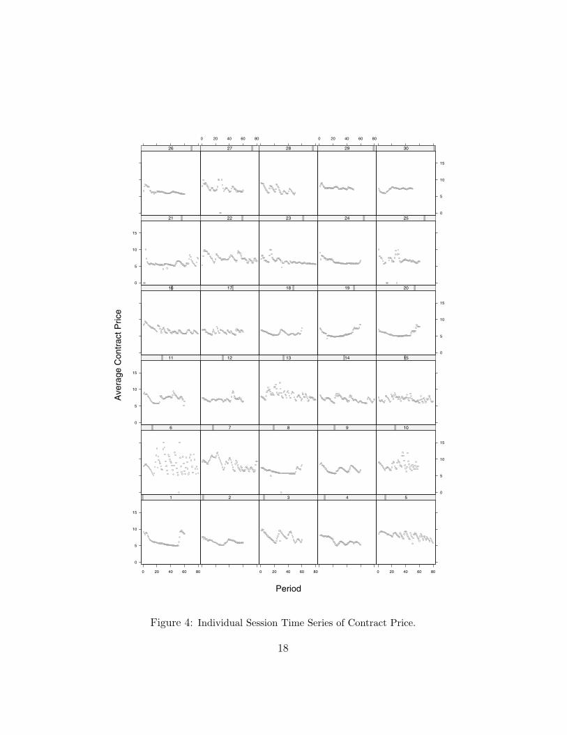
In Figure 4 we provide the time series of average contract price for eachexperimental session. Inspection of these series clearly reveals that Edge-worth style cyclical patterns are a common characteristic in many of thesessions. However there does not appear to be any consistent pattern orstatistical regularity.

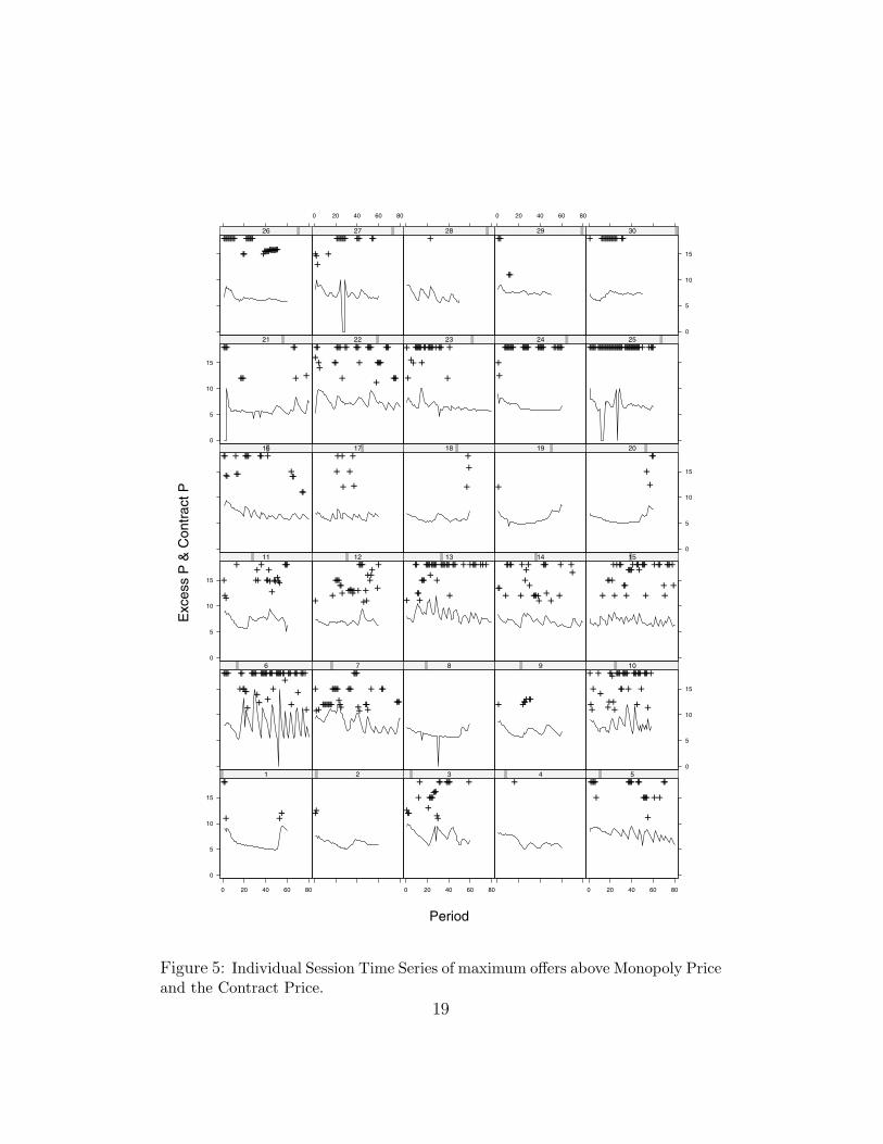
Finally, Figure 5, which plots the individual maximum offer prices thatare greater than the monopoly price, as well as the mean contract price in

17

0

5

10

15

0 20 40 60 80

1 2

0 20 40 60 80

3 4

0 20 40 60 80

5

6 7 8 9

0

5

10

15

100

5

10

15

11 12 13 14 15

16 17 18 19

0

5

10

15

200

5

10

15

21 22 23 24 25

26

0 20 40 60 80

27 28

0 20 40 60 80

29

0

5

10

15

30

Period

Ave

rage

Con

trac

t Pric

e

Figure 4: Individual Session Time Series of Contract Price.

18

0

5

10

15

0 20 40 60 80

1++

+ ++

2

++

0 20 40 60 80

3

+++++

++++++++

++

++++++ +4

+

0 20 40 60 80

5++++++

++++++++++

+

++++

6+++++

++++++++

+++++

++

++++++

+

+++++++++++

++++

+

+++

+

++++

+

7

+

++++++++++++++++++++

+++++++

+++++

+ +++++

8 9

+ ++++++

0

5

10

15

10+

++

++

+++

+++

++

+++++++++++++++

+

+++++++

+

+0

5

10

15

11

+++

+++++++++++++++

+++12

+ +++++++

++++++++

++++

+++

++++

+

+13

+

++

+++

+++++++++++++++++++++

+

+++ ++++++++14

+++

++++

+

++++

++++++

+++

++ +

+ ++

15

+++++

+

+++

+++

+++++++++++

+

+++

++

++++

+

16++

++

+

++

++++ ++++++

++

17

+++

+++

+

18

+

++

19

+

0

5

10

15

20

++

++0

5

10

15

21++++

+++

++

+ +

22

+++++ ++

++++

+

++ ++++

++++

+

+++++++

+++

23+

+

++++++++++++++++++++

+

+24

++

+++++++++ ++++++ ++++++ +++++++25

++++++++++++++++++++++++++++++++++++++++++++++++

26+++++++++++

+++++++++

++++++++++++++

0 20 40 60 80

27

+++

++++++++++ +++ ++

28+

0 20 40 60 80

29+++

++

0

5

10

15

30+ +++++++++++++++++

Period

Exc

ess

P &

Con

trac

t P

Figure 5: Individual Session Time Series of maximum offers above Monopoly Priceand the Contract Price.

19

each period, indicates that signaling at absurdly high prices was extremelycommon.

6 Conclusions

In environments where decision-makers face both sunk and avoidable fixedcosts, we observe a pattern of price signaling and responses which main-tain above normal profits; firms succeed, even through their joint conductis clearly very competitive. This success means that firm’s do not have toexit such an industry in order to avoid loses (or for the industry to maintainprofitability), and may help to explain why some competitive industries ap-pear to maintain an inefficient number of firms over much longer periods oftime than expected. However, in our experimental environment, we cannotreject the hypothesis that the fixed cost treatment has no effect on prices.This finding is consistent, however, with the standard economic principlethat fixed costs should not affect decision making at the margin.

A closer examination of the data suggests that the form of competitionfirms engage in is responsible for their profitability. Below the Ramsey price,losses are incurred, and the alternative, since the firm is already incurringlosses, is to raise its price. This unilateral action produces zero sales, andavoids all but the sunk cost. However, by setting a higher price in this perioda firm hopes that other firms will raise their prices next period. Why don’tfirms see this as a ruse by the signaling firm? By offering a higher price in aperiod, a firm may be committing to a price in the next period, perhaps lowerthan its signal, but greater than its price in the previous period. Formally,the commitment in the next period must take the form of a mixed strategyto ensure that the other firms are unable to predict and simply undercut thesignaler’s price. Other firms in the same position, would then have a strongincentive to raise their prices as they trade off the cost of being the firmleft out of the market in the next period against the benefit of more profits.Firms will maintain positive profits if they can work out a repeated responsethat allows each to partake of profits on various occasions. For example,as long as firms’ price responses are sufficiently randomized and prices stayabove the Ramsey price, different firms will be rationed each period, but theirlosses in these periods will be outweighed by increased profits in periods inwhich they sell.

20

References

[1] Buchheit, Steve and Nick Feltovich, (200). “The Relationship BetweenSunk Costs and Firms’ Firms Pricing Decisions: An Experimental Study”.Mimeo, University of Houston, October.

[2] Durham, Yvonne, Stephen J. Rassenti, Vernon L. Smith, Mark Van Boen-ing and National T. Wilcox, (1996). “Can Core Allocations Be Achievedin Avoidable Fixed Cost Environments Using Two-Part Pricing Compe-tition?”, Annals of Operations Research, Special Issue on ComputationalEconomics, edited by S. Thore and G. Thompson, Vol. 68, August, 61–88.

[3] Friedman, James W. and Austin C. Hoggatt, (1980). An Experiment inNon-cooperative Oligopoly, Greenwich, Conn: JAI Press Inc.

[4] Ketcham, Jon, Vernon L. Smith, and Arlington Williams, (1984). “AComparison of Posted-Offer and Double-Auction Pricing Institutions,” Re-view of Economic Studies 51: 595–614.

[5] Kruse, Jamie B., (1991). “Contestability in the Presence of an AlternateMarket: An Experimental Evaluation,” Rand Journal of Economics 22:Spring, 136–147.

[6] Kruse, Jamie B., Stephen J. Rassenti, Stanley S. Reynolds and Vernon L.Smith, (1994). “Bertrand–Edgeworth Competition in Experimental Mar-kets,” Econometrica 62: March, 343–371.

[7] Laird, N. M. and J. H. Ware (1982). “Random-effects models for longi-tudinal data”, Biometrics 38: 963–974.

[8] Martin, Stephen (2003). “Globalization and the Natural Limits of Com-petition”, Mimeo, Department of Economics, Purdue University, January.

[9] Offerman, Theo and Jan Potters (2002). “Does Auctioning of Entry Li-censes Induce Collusion? An Experimental Study”. Mimeo, CREED, Uni-versity of Amsterdam, September.

[10] Smith, Vernon L. (1974). “Optimal Costly Firm Entry in General Equi-librium,” Journal of Economic Theory, December.

[11] Telser, L. G., (1988). A Theory of Efficient Cooperation and Competi-tion, Cambridge: Cambridge University Press.

21

[12] Van Boening, Mark V. and Nathaniel T. Wilcox, (1996). “AvoidableCost: Ride a Double Roller Coaster,” American Economic Review 6,3:,June, 461–477.

22