Competition and Market Strategies in the

Swiss Fixed Telephony Market

An estimation of the incumbent’s

dynamic residual demand curve

Roberto Balmer

Bundesamt für Kommunikation

Disclaimer: The views presented here are those of the author and do not reflect those of BAKOM.

Biennial Conference

International Telecommunications Society

1 December 2014

Link to working paper

2

Market and Assumptions (1/2)The question:

• Retail fixed telephony regulation lifted in many European States

• Sufficient competition?

• Demand/supply model for Switzerland 2004-2012

The challenge:

• Highest frequency data available is usually quarterly (few data points)

• Complexity of market model strongly limited

Strong simplifications:

1) No vertical integration issues:

Identical network origination costs are assumed across competitors (access at efficient marginal costs for access seekers and infrastructure-based operators). LRIC prices therefore assumed to be close to marginal cost (exogenous).

2) Two-way access:

a) Regulated fixed termination rates (LRIC) are close to zero (<1€cent/min). No fixed termination costs & revenues modeled.

b) Mobile termination rates are unregulated in Switzerland. Rate modeled as exogenous cost shifters for fixed operators (>10€cent/min).

1. Introduction 2. Model 3. Variables 4. Conclusions

3

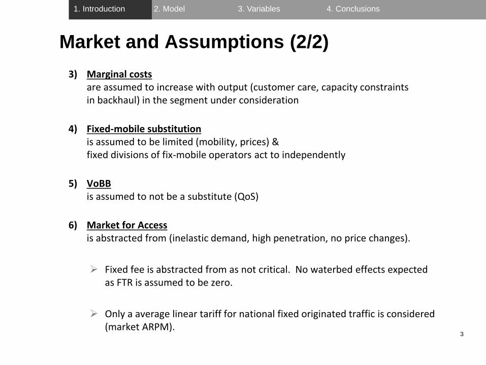
Market and Assumptions (2/2)

3) Marginal costs are assumed to increase with output (customer care, capacity constraints in backhaul) in the segment under consideration

4) Fixed-mobile substitutionis assumed to be limited (mobility, prices) &fixed divisions of fix-mobile operators act to independently

5) VoBBis assumed to not be a substitute (QoS)

6) Market for Accessis abstracted from (inelastic demand, high penetration, no price changes).

Fixed fee is abstracted from as not critical. No waterbed effects expected as FTR is assumed to be zero.

Only a average linear tariff for national fixed originated traffic is considered (market ARPM).

1. Introduction 2. Model 3. Variables 4. Conclusions

4

Traditional model assuming a particular way how firms compete:

• Dominant firm takes the reaction of the fringe firms into account when deciding on quantity and price

• Fringe firms are assumed to be pure price takers ( )

• Fringe supply is therefore given by sum of fringe marginal cost curves.

• Incumbent Swisscom maximizes profitability with Q and P such that

MR(residual demand)=MC (Swisscom)

Fcp

Dominant firm – Competitive Fringe (1/3)

1. Introduction 2. Model 3. Variables 4. Conclusions

DM is the market demand curve (Q is total

demand)

𝑆𝐹 is the fringe supply curve (𝑄𝐹 is fringe supply)

𝐷𝑅𝑒𝑠𝑖𝑑𝑢𝑎𝑙 is the residual demand curve that the dominant

firm faces (𝑄𝐷 is dominant firm demand)

𝑀𝑅𝑅𝑒𝑠𝑖𝑑𝑢𝑎𝑙 is the residual marginal revenue curve the

dominant firm faces

𝐶𝐷 is the dominant firm’s marginal costs

𝑃 is the unique market price

5

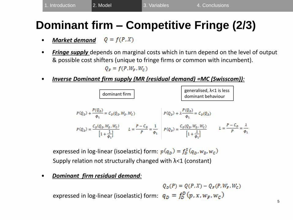
Dominant firm – Competitive Fringe (2/3)• Market demand

• Fringe supply depends on marginal costs which in turn depend on the level of output & possible cost shifters (unique to fringe firms or common with incumbent).

• Inverse Dominant firm supply (MR (residual demand) =MC (Swisscom)):

expressed in log-linear (isoelastic) form:

Supply relation not structurally changed with λ<1 (constant)

• Dominant firm residual demand:

expressed in log-linear (isoelastic) form:

1. Introduction 2. Model 3. Variables 4. Conclusions

dominant firmgeneralised, λ<1 is lessdominant behaviour

6

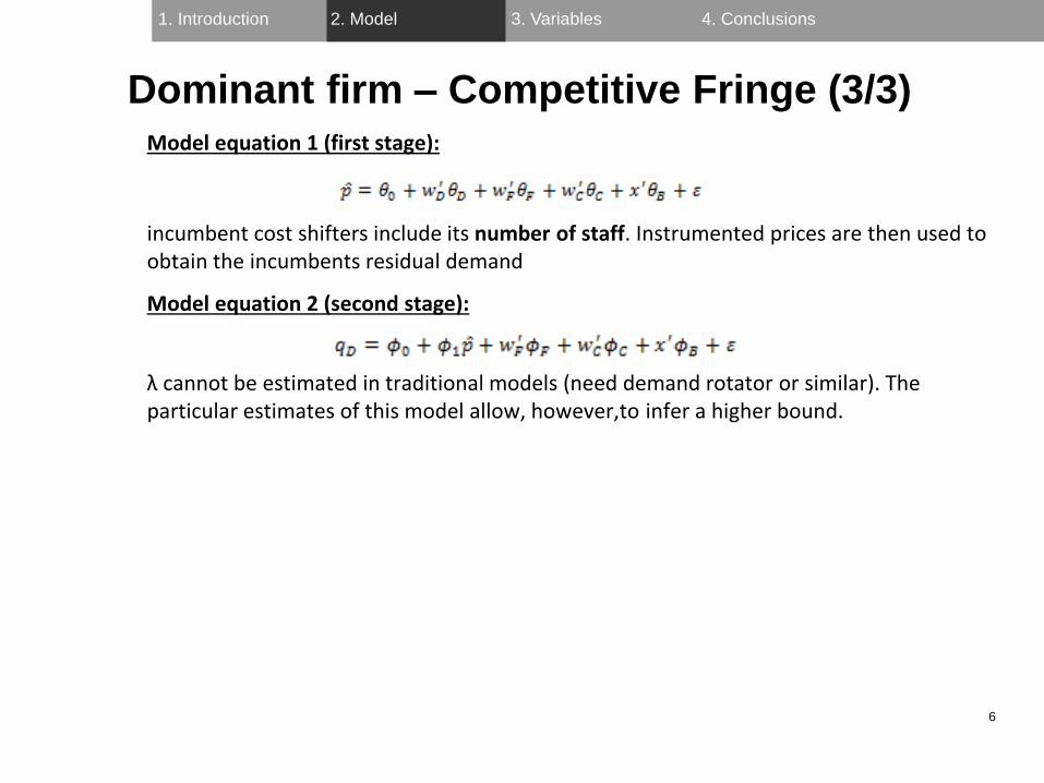
Model equation 1 (first stage):

incumbent cost shifters include its number of staff. Instrumented prices are then used to obtain the incumbents residual demand

Model equation 2 (second stage):

λ cannot be estimated in traditional models (need demand rotator or similar). The particular estimates of this model allow, however,to infer a higher bound.

Dominant firm – Competitive Fringe (3/3)

1. Introduction 2. Model 3. Variables 4. Conclusions

7

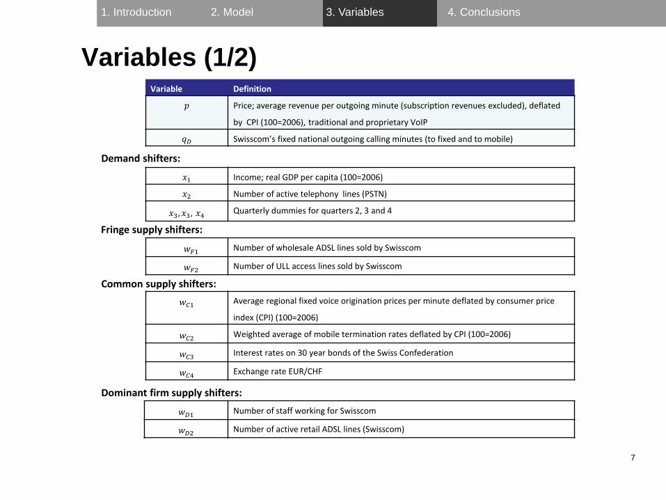
Variable Definition

𝑝 Price; average revenue per outgoing minute (subscription revenues excluded), deflated

by CPI (100=2006), traditional and proprietary VoIP

𝑞𝐷 Swisscom’s fixed national outgoing calling minutes (to fixed and to mobile)

𝑥1 Income; real GDP per capita (100=2006)

𝑥2 Number of active telephony lines (PSTN)

𝑥3, 𝑥3, 𝑥4 Quarterly dummies for quarters 2, 3 and 4

𝑤𝐹1 Number of wholesale ADSL lines sold by Swisscom

𝑤𝐹2 Number of ULL access lines sold by Swisscom

𝑤𝐶1 Average regional fixed voice origination prices per minute deflated by consumer price

index (CPI) (100=2006)

𝑤𝐶2 Weighted average of mobile termination rates deflated by CPI (100=2006)

𝑤𝐶3 Interest rates on 30 year bonds of the Swiss Confederation

𝑤𝐶4 Exchange rate EUR/CHF

𝑤𝐷1 Number of staff working for Swisscom

𝑤𝐷2 Number of active retail ADSL lines (Swisscom)

Demand shifters:

Fringe supply shifters:

Common supply shifters:

Dominant firm supply shifters:

Variables (1/2)

1. Introduction 2. Model 3. Variables 4. Conclusions

8

Econometrical problems

• Variables p and q decline over time (non-stationarity)

• Errors are serially correlated

Solution

To avoid spurious regression results: ARDL(1,1)

• Sufficient level of cointegration

• No serial correlation

Variables (2/2)

1. Introduction 2. Model 3. Variables 4. Conclusions

9

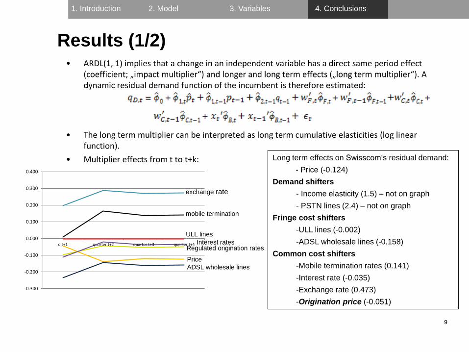
• ARDL(1, 1) implies that a change in an independent variable has a direct same period effect (coefficient; „impact multiplier“) and longer and long term effects („long term multiplier“). A dynamic residual demand function of the incumbent is therefore estimated:

• The long term multiplier can be interpreted as long term cumulative elasticities (log linear function).

• Multiplier effects from t to t+k:

-0.300

-0.200

-0.100

0.000

0.100

0.200

0.300

0.400

q t+1 quarter t+2 quarter t+3 quarter t+4

Results (1/2)

exchange rate

mobile termination

ADSL wholesale lines

Price

Regulated origination ratesInterest rates

Long term effects on Swisscom‘s residual demand:

- Price (-0.124)

Demand shifters

- Income elasticity (1.5) – not on graph

- PSTN lines (2.4) – not on graph

Fringe cost shifters

-ULL lines (-0.002)

-ADSL wholesale lines (-0.158)

Common cost shifters

-Mobile termination rates (0.141)

-Interest rate (-0.035)

-Exchange rate (0.473)

-Origination price (-0.051)

ULL lines

1. Introduction 2. Model 3. Variables 4. Conclusions

10

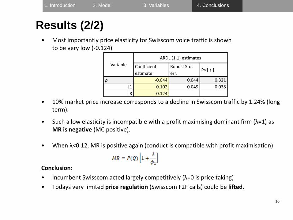
• Most importantly price elasticity for Swisscom voice traffic is shownto be very low (-0.124)

• 10% market price increase corresponds to a decline in Swisscom traffic by 1.24% (longterm).

• Such a low elasticity is incompatible with a profit maximising dominant firm (λ=1) asMR is negative (MC positive).

• When λ<0.12, MR is positive again (conduct is compatible with profit maximisation)

Conclusion:

• Incumbent Swisscom acted largely competitively (λ=0 is price taking)

• Todays very limited price regulation (Swisscom F2F calls) could be lifted.

Variable

ARDL (1,1) estimates

Coefficient

estimate

Robust Std.

err.P>| t |

p -0.044 0.044 0.321

L1 -0.102 0.049 0.038

LR -0.124

Results (2/2)

1. Introduction 2. Model 3. Variables 4. Conclusions

11

Questions?

Dr. Roberto Balmer

Bundesamt für Kommunikation

TC / Sektion Ökonomie

Zukunftstr. 44

2501 Biel

Switzerland

Tel. +41 32 327 56 43

roberto.balmer@bakom.admin.ch

linkedin.com/in/RobertoBalmer

slideshare.net/RobertoBalmer

amazon.com/author/roberto.balmer

ssrn.com/author=572707

1. Introduction 2. Model 3. Variables 4. Conclusions

12

Backup

1. Introduction 2. Model 3. Variables 4. Conclusions

13

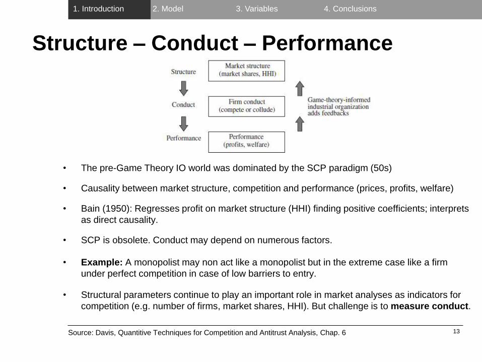
Structure – Conduct – Performance

Source: Davis, Quantitive Techniques for Competition and Antitrust Analysis, Chap. 6

• The pre-Game Theory IO world was dominated by the SCP paradigm (50s)

• Causality between market structure, competition and performance (prices, profits, welfare)

• Bain (1950): Regresses profit on market structure (HHI) finding positive coefficients; interprets

as direct causality.

• SCP is obsolete. Conduct may depend on numerous factors.

• Example: A monopolist may non act like a monopolist but in the extreme case like a firm

under perfect competition in case of low barriers to entry.

• Structural parameters continue to play an important role in market analyses as indicators for

competition (e.g. number of firms, market shares, HHI). But challenge is to measure conduct.

1. Introduction 2. Model 3. Variables 4. Conclusions

14

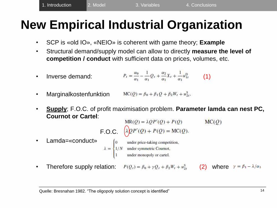
New Empirical Industrial Organization

• SCP is «old IO», «NEIO» is coherent with game theory; Example

• Structural demand/supply model can allow to directly measure the level of

competition / conduct with sufficient data on prices, volumes, etc.

• Inverse demand: (1)

• Marginalkostenfunktion

• Supply; F.O.C. of profit maximisation problem. Parameter lamda can nest PC,

Cournot or Cartel:

F.O.C.

• Lamda=«conduct»

• Therefore supply relation: (2) where

Quelle: Bresnahan 1982. “The oligopoly solution concept is identified”

1. Introduction 2. Model 3. Variables 4. Conclusions

15

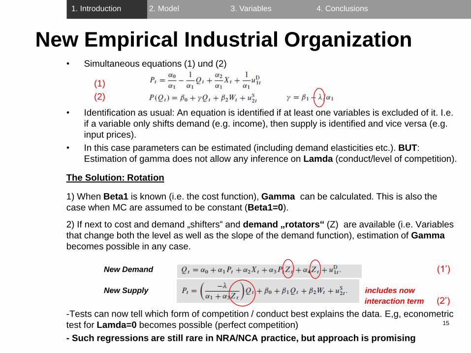
• Simultaneous equations (1) und (2)

(1)

(2)

• Identification as usual: An equation is identified if at least one variables is excluded of it. I.e.

if a variable only shifts demand (e.g. income), then supply is identified and vice versa (e.g.

input prices).

• In this case parameters can be estimated (including demand elasticities etc.). BUT:

Estimation of gamma does not allow any inference on Lamda (conduct/level of competition).

The Solution: Rotation

1) When Beta1 is known (i.e. the cost function), Gamma can be calculated. This is also the

case when MC are assumed to be constant (Beta1=0).

2) If next to cost and demand „shifters“ and demand „rotators“ (Z) are available (i.e. Variables

that change both the level as well as the slope of the demand function), estimation of Gamma

becomes possible in any case.

New Demand (1’)

New Supply includes now

interaction term (2’)

-Tests can now tell which form of competition / conduct best explains the data. E,g, econometric

test for Lamda=0 becomes possible (perfect competition)

- Such regressions are still rare in NRA/NCA practice, but approach is promising

New Empirical Industrial Organization

1. Introduction 2. Model 3. Variables 4. Conclusions