Embed Size (px)
Citation preview

SEAT BELT OBSERVATION STUDY
SUMMER 2006
Thomas E. James, Ph.D., DirectorKathy Hall, Assistant Director
Matthew Krimmer, Graduate Research Assistant
Institute for Public AffairsUniversity of Oklahoma
455 W. Lindsey Street, Room 304Norman, Oklahoma 73019-2002
July 2006
This report was prepared for the Oklahoma Highway Safety Office in cooperation with the National Highway Traffic
Safety Administration, U.S. Department of Transportation and/or Federal Highway Administration, U.S. Department
of Transportation. The conclusions and opinions expressed in this report are those of the Institute for Public Affairs, and
do not necessarily represent those of the State of Oklahoma, the Oklahoma Highway Safety Office, the U.S. Department
of Transportation, or any other agency of the State or Federal Government.

TABLE OF CONTENTS
Page Number
Executive Summary ..................................................................................................................... iii
Introduction .................................................................................................................................... 1
Study Methodology ........................................................................................................................ 1
Results of the Survey ..................................................................................................................... 6
Summary and Recommendations ................................................................................................. 13
Endnotes ....................................................................................................................................... 15
References .................................................................................................................................... 16
Appendix A: Seat Belt Observation Sites ...................................................................... 17Appendix B: Estimation and Analysis Procedures ........................................................ 26Appendix C: Random Assignment of Observers .......................................................... 28Appendix D: Instructions for Observing Safety Belt Use .............................................. 29Appendix E: Seat Belt Observation Data Collection Form ........................................... 30
LIST OF TABLES
Table 1: Sample Sites by Region, County, Metropolitan Areas and Roadways .................. 3
Table 2: Estimate of Seat Belt Use in Oklahoma: Summer 2006 ........................................ 6
Table 3: Estimated Seat Belt Use in Oklahoma By Type of Vehicle: Summer 2006 .......... 7
Table 4: Estimate of Seat Belt Use in Oklahoma by County: Summer 2006 ...................... 9
Table 5: Comparison of Seat Belt Use in Oklahoma: 2002-2006 ...................................... 11
Table 6: Estimate of Seat Belt Use in Oklahoma by Gender and Race: Summer 2006 ..... 12

iii
EXECUTIVE SUMMARY
The 2006 statewide survey of safety belt use in Oklahoma was conducted in 19 counties at315 observation sites during the month of June. The sampling procedures replicated the approachinitially adopted in winter of 1991-1992 and followed in each statewide survey thereafter. Thedesign is a random probability sample based on population and average daily vehicle miles traveled(DVMT). The design was a statewide, multistage, area sample of roadway segments and localroadway intersections. Beginning with the 2002 survey, a new set of sample sites was selected using2000 Census data and 2000 DVMT data. Given that the design was a random probability sample,the data analyses used a weighted ratio of belted drivers and belted front-seat outboard passengersto the total number of drivers and front-seat outboard passengers observed.
In 2006, a total of 42,761 drivers and front-seat outboard passengers were observed. Of thetotal individuals observed, 19,356 were traveling in passenger cars (45.3 percent of the sample),3,943 were traveling in vans (9.2 percent), 8,154 were in SUVs/Jeeps (19.1 percent), and 11,308were traveling in pickup trucks (26.4 percent). In previous years, survey results reported seatbeltusage for pickups compared to all other categories of vehicles combined under “automobiles”. Thus,for the purpose of comparison with previous surveys, results will include an “automobile” categorywhich simply sums the results from all vehicles that are not pickup trucks (cars, vans, andSUVs/Jeeps).
Estimated Seat Belt Use for Drivers and Front-Seat Outboard Passengersin Oklahoma: Summer 2006
Weighted Percent
Combined Autos Cars Vans SUVs Pickups1
Statewide 83.7 86.4 86.7 87.1 85.3 75.9
Regions (non-metropolitan)
West 83.6 85.8 85.2 89.2 85.0 77.8
Northeast 80.0 83.6 83.0 83.9 84.6 71.9
Southeast 79.9 84.9 85.2 86.4 83.5 69.5
Metropolitan Counties
Oklahoma 81.3 83.4 84.2 85.0 81.1 73.1
Tulsa 90.7 92.6 93.2 90.7 91.8 84.5
NOTE:
The ‘auto’ category sums the results from all vehicles that are not pickup trucks (cars, vans, and SUVs/Jeeps).1

iv
A comparison of the summer 2005 and the summer 2006 survey results reveals that statewidesafety belt use increased by a statistically significant 0.6 of a percentage point (from 83.1 percentto 83.7 percent). The usage rate for summer 2006 is the highest since the summer of 1998 whenweighted data began to be used. All five regions experienced an increase in seatbelt use over 2002with the largest increase in Tulsa County (18.2 percentage points).
As noted by Glassbrenner (2004), improvement in belt use generally is measured by thepercentage point increase in the use rate. However, the same percentage point increase for twodifferent areas is not always equivalent. Increasing the use rate by 2 percentage points from a baseof 85 percent is more difficult than increasing by the same amount if an area is starting at a 50percent use rate. Increasing use from 85 percent requires changing the behavior of a larger fractionof nonusers. Consequently, NHTSA has begun calculating a measure termed the “conversion rate,”the percentage of nonusers that were converted to users (the percentage reduction in nonuse).Beginning with the summer 2004 report, the conversion rate is included for Oklahoma. Statewide,the 0.6 percentage point increase from 2005 to 2006 is equivalent to a 3.6 percent decrease innonusers. Reduction of nonusers occurred in Tulsa County (33.1 percent) and the Northeast region(13.4 percent). Between the 2002 and 2006 surveys, belt nonuse statewide was reduced by 45.5percent.
The difference in safety belt use between automobiles (cars, vans, SUVs, Jeeps) and pickuptrucks continues to be substantial. Statewide safety belt use in automobiles reached 86.7 percent,while only 75.9 percent of drivers and front-seat outboard passengers were belted in pickups.Because pickup observations account for 26.4 percent of all observations, the low rate of buckleddrivers and passengers in pickup trucks substantially lowers the overall use rate for the state.
With respect to race, the 2006 results indicate that non-white drivers and passengers areslightly more likely to buckle than whites (84.4 percent versus 82.8 percent). Differences also areevident when males and females are compared. Women buckled up at a rate of 87.5 percent,whereas men used seat belts at a rate of 79.8 percent. The lower use rate for men is, in part, due tothe low buckled rate for those driving or riding in pickup trucks; 38 percent of male drivers andpassengers were observed in pickups and their use rate was 73 percent.

1
OKLAHOMA SEAT BELT OBSERVATION STUDYSUMMER 2006
INTRODUCTIONDuring June 2006, the Institute for Public Affairs at the University of Oklahoma (OU)
undertook a statewide observation survey of safety belt use in Oklahoma. The survey has beenconducted through OU since 1986 and is part of an ongoing effort to evaluate the effectiveness ofthe Oklahoma Mandatory Seat Belt Use Act (Title 47, Chapter 12, § 416-421).
Oklahoma's law requiring automobile drivers and front-seat passengers to buckle up becameeffective February 1, 1987. It was amended on February 1, 1989 to require drivers and front-seatpassengers of pickup trucks and vans to wear seat belts as well. Until the enactment of House Bill1443 in 1997, Oklahoma's law permitted only "secondary enforcement." An unbelted driver couldbe ticketed only after being stopped for another traffic violation. The 1997 law permits primaryenforcement – a law enforcement officer can issue a citation solely for failure to buckle up.Oklahoma has joined 20 other states and the District of Columbia with primary enforcement laws(Glassbrenner, 2004).
The 2006 survey included 315 observation sites, resulting in 42,761 drivers and front-seatoutboard passengers being observed for safety belt use. This report presents the results of thesummer 2006 survey and compares these findings with the results of similar statewide surveysconducted during the previous four years.
STUDY METHODOLOGYThis section describes the process used to sample and allocate sites for observation and
procedures for observation and data collection, weighting and data analysis, and observer selectionand training. The survey findings are presented following the discussion of the study methodology.
Observation Site Selection and AllocationBeginning with the winter 1991-92 study and for all subsequent surveys, a probability-based
design was followed to ensure the potential selection of any road intersection in the state as anobservation site. The sample was drawn using a statewide, multistage, area probability sample ofroad segments and intersections. In 1999, the sample was modified slightly by dropping threecounties. The new 19 county sample reflected three non-metropolitan regions and Tulsa and1
Oklahoma Counties. Tulsa and Oklahoma Counties were designated as "certainty" counties to beincluded in the sample because of their high levels of daily vehicle miles traveled (DVMT). Theycontain the two largest cities in the state, so together they provide a measurement of safety belt usein the largest metropolitan areas.
To increase comparability across surveys, the same site locations were used from the 1991-1992 survey through the 2001 survey. Due to road construction and population changes during thattime period, a decision was made to update the original sample for the 2002 survey. The method

2
used to draw the sample of sites for 2002 mirrored the procedure used previously. Population datafor counties was taken from the 2000 Census and daily vehicle miles traveled data for 2000 (thelatest available) were provided by the Oklahoma Department of Transportation.
Counties in the non-certainty category, representing smaller communities and rural areas,were weighted by population and 17 were randomly selected. Six counties were selected for theNortheast and six for the Southeast region, while five counties were selected in the West region.Excluding Tulsa and Oklahoma Counties, the number of sample counties selected per region reflectsthat region's population. This resulted in one county less in the Northeast and one county more inthe West compared to the previous sample.
The sample included 315 observation sites statewide (see Appendix A for a complete list).Sixty percent of the sites were allocated to major roads and 40 percent to local roads, to reflect thedistribution of daily vehicle miles traveled between the two types of roadways (the actualdistribution of DVMT is 38 percent local roads and 62 percent major). Therefore, in each of the 17non-metropolitan counties sampled, 15 observation sites were selected with nine allocated to majorroads and six to local roads. In the largest sample counties, the Tulsa and Oklahoma Citymetropolitan areas, 30 observation sites were allocated with 18 sites on major roads and 12 on localroads. The allocation by region, county, and metropolitan area is summarized in Table 1.
Following the 1991 methodology, the procedure for selecting roadway sites differedaccording to whether they were major roadways (interstates, U.S. roads, and state roads) or localroadways (all other paved roads, excluding reservations, airports, and privately controlled areas).Major roadway sites were selected by weighting the road segment lengths by the traffic volume andthen randomly selecting the road segment in each county. Data for major road segments wereprovided by the Oklahoma Department of Transportation. Observation sites were determined byselecting the intersection or location nearest to where each road segment began and from whichsafety belt use could be readily observed.
Local roadway sites were determined by first weighting the census tracts based onpopulation, and then randomly selecting the three census tracts in each county. County and localroadway intersections, as identified on the county maps in each of the selected census tracts, wererandomly selected. The only sites considered were those in which three or more road segmentsjoined together. In towns and communities with residential streets, only the main arteries wereincluded in the pool to be sampled.
The data collected from these randomly selected observation sites were used to calculate theconfidence interval for each of the categories in the sample. The confidence interval describes thevariability of the data within each category caused by sampling design and provides a value usedto calculate a range or interval in which the population's actual seat belt usage can be estimated. A95 percent confidence level is calculated by multiplying an estimate of the standard error by 1.96.The standard error is estimated using a balanced repeated replication technique described inAppendix B.

3
Table 1 Sample Sites by Region, County, Metropolitan Areas and Roadways
Number of Sites Major Roads Local Roads
Statewide Totals 315 189 126
Regions (non-metropolitan)
West 75 45 30
Canadian 15 9 6
Comanche 15 9 6
Garfield 15 9 6
Grady 15 9 6
Logan 15 9 6
Northeast 90 54 36
Delaware 15 9 6
Mayes 15 9 6
Muskogee 15 9 6
Ottawa 15 9 6
Payne 15 9 6
Rogers 15 9 6
Southeast 90 54 36
Bryan 15 9 6
Carter 15 9 6
Cleveland 15 9 6
McClain 15 9 6
Pontotoc 15 9 6
Pottawatomie 15 9 6
Metropolitan Counties 60 36 24
Oklahoma 30 18 12
Tulsa 30 18 12

4
Observation and Data Collection Procedures Assignment of Observers. All daylight hours for all days of the week were eligible for inclusion inthe sample. Appendix C provides a more complete description of the methodology for randomassignment of observers to each location. The basic procedure for random assignment of observersby day of week and time of day was as follows:
1. With 15 sites per county, it was assumed that observers would cover one county in two days– eight locations in day 1 and seven locations in day 2.
2. The earliest start time was set at 7:00 a.m. and the last start time was determined to be 11:00a.m. (the 11a.m. time would assure that the observer would complete all observations by nolater than 7:00 p.m.; 11 + 8 = 19; 1900 hours; 7 p.m.).
3. The counties were assigned to three non-metropolitan regions (West, Northeast, Southeast)and two metropolitan counties (Tulsa and Oklahoma).
4. Observers were provided a predetermined sequence of counties in each region to minimizetravel time.
5. The sequencing of sites within each county also was predetermined to form a rough circleof sites that could be covered in a single day, again to minimize travel time.
6. The beginning day of the week was decided by a roll of a die.
7. Observers were told from which corner of the intersection they would observe.
Data Collection Procedures. At all sites, observers collected the following data for drivers and front-seat outboard passengers (see Appendix D for further discussion):
• Time of day
• Date
• Type of vehicle (car/van/SUV/Jeep/pickup truck)
• Shoulder belt use (using/not using)
• Gender (male/female/unsure)
• Race (white/non-white/unsure)
5
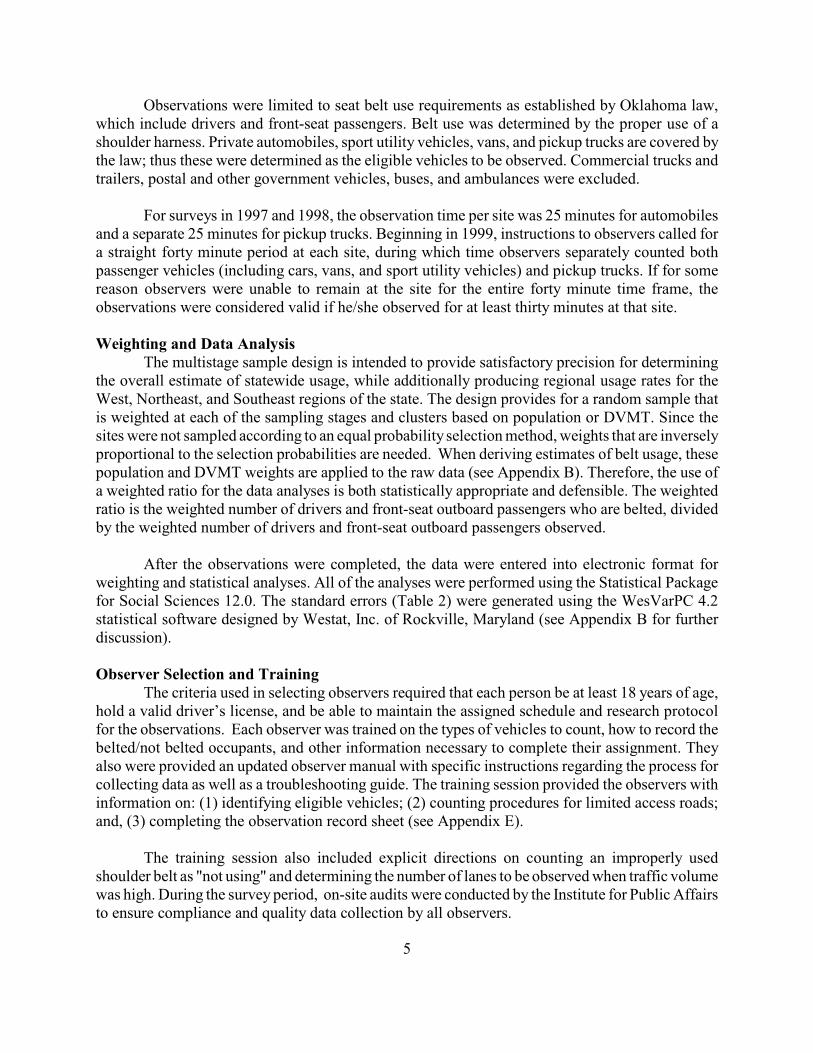
Observations were limited to seat belt use requirements as established by Oklahoma law,which include drivers and front-seat passengers. Belt use was determined by the proper use of ashoulder harness. Private automobiles, sport utility vehicles, vans, and pickup trucks are covered bythe law; thus these were determined as the eligible vehicles to be observed. Commercial trucks andtrailers, postal and other government vehicles, buses, and ambulances were excluded.
For surveys in 1997 and 1998, the observation time per site was 25 minutes for automobilesand a separate 25 minutes for pickup trucks. Beginning in 1999, instructions to observers called fora straight forty minute period at each site, during which time observers separately counted bothpassenger vehicles (including cars, vans, and sport utility vehicles) and pickup trucks. If for somereason observers were unable to remain at the site for the entire forty minute time frame, theobservations were considered valid if he/she observed for at least thirty minutes at that site.
Weighting and Data AnalysisThe multistage sample design is intended to provide satisfactory precision for determining
the overall estimate of statewide usage, while additionally producing regional usage rates for theWest, Northeast, and Southeast regions of the state. The design provides for a random sample thatis weighted at each of the sampling stages and clusters based on population or DVMT. Since thesites were not sampled according to an equal probability selection method, weights that are inverselyproportional to the selection probabilities are needed. When deriving estimates of belt usage, thesepopulation and DVMT weights are applied to the raw data (see Appendix B). Therefore, the use ofa weighted ratio for the data analyses is both statistically appropriate and defensible. The weightedratio is the weighted number of drivers and front-seat outboard passengers who are belted, dividedby the weighted number of drivers and front-seat outboard passengers observed.
After the observations were completed, the data were entered into electronic format forweighting and statistical analyses. All of the analyses were performed using the Statistical Packagefor Social Sciences 12.0. The standard errors (Table 2) were generated using the WesVarPC 4.2statistical software designed by Westat, Inc. of Rockville, Maryland (see Appendix B for furtherdiscussion).
Observer Selection and TrainingThe criteria used in selecting observers required that each person be at least 18 years of age,
hold a valid driver’s license, and be able to maintain the assigned schedule and research protocolfor the observations. Each observer was trained on the types of vehicles to count, how to record thebelted/not belted occupants, and other information necessary to complete their assignment. Theyalso were provided an updated observer manual with specific instructions regarding the process forcollecting data as well as a troubleshooting guide. The training session provided the observers withinformation on: (1) identifying eligible vehicles; (2) counting procedures for limited access roads;and, (3) completing the observation record sheet (see Appendix E).
The training session also included explicit directions on counting an improperly usedshoulder belt as "not using" and determining the number of lanes to be observed when traffic volumewas high. During the survey period, on-site audits were conducted by the Institute for Public Affairsto ensure compliance and quality data collection by all observers.

6
RESULTS OF THE SURVEYDuring June 2006, observers visited the 315 sites in the 19 sample counties. They collected
data for 42,761 drivers and front-seat outboard passengers. Of those observations, 19,356 weretraveling in passenger cars (45.3 percent of the sample), 3,943 were traveling in vans (9.2 percent),8,154 were in SUVs/Jeeps (19.1 percent), and 11,308 were traveling in pickup trucks (26.4 percent).Drivers accounted for 33,637 (78.7 percent) of the observations and 9,124 (21.3 percent) werepassengers.
Table 2 shows the estimates of safety belt use and confidence intervals for the state, non-metropolitan regions, the two metropolitan counties, and roadway types (major and local). Thestatewide seat belt usage rate for drivers and front-seat outboard passengers was 83.7 percent. TulsaCounty led all regions with 90.7 percent buckled up. The Southeast region had the lowest percentage
Table 2 Estimate of Seat Belt Use in Oklahoma:
Summer 2006
UnweightedObservations
WeightedEstimate
(PERCENT)
StandardError
(PERCENT)
ConfidenceInterval*
(PERCENT)
Statewide 42,761 83.7 .3 +/-.6
Regions (non-metropolitan)
West 8,221 83.6 1.5 +/-2.9
Northeast 10,677 80.0 .3 +/-.6
Southeast 7,877 79.9 .1 +/-.6
Metropolitan Counties
Oklahoma 8,841 81.3 1.7 +/-3.3
Tulsa 7,145 90.7 2.4 +/- 4.7
Roadway Type
Major 30,097 83.5 2.7 +/-5.3
Local 12,664 83.5 3.1 +/-6.1
*The confidence interval is also sometimes referred to as sampling error. Based on a 95 percent confidence level, the
actual belt use for each category shown in the table is the estimated percentage use + or – the standard error (S.E.)
multiplied by 1.96. For example, for the state as a whole, the actual percentage use should be between 83.1 and 84.3
percent [83.7 +/- (1.96 x .3)] for 95 samples out of 100.

7
buckled (79.9 percent). The drivers and passengers observed statewide were no more likely to usea seat belt when traveling on major roads than when driving on local roadways (83.5 percent).
The differences in seat belt use by the type of vehicle are presented in Table 3. For the entirestate, 86.4 percent of drivers and passengers in automobiles (includes cars, vans, and sport utilityvehicles/Jeeps) were buckled up, while 75.9 percent were restrained in pickup trucks. Drivers andpassengers in vans were the most likely to be buckled up (87.1 percent), followed by those in cars(86.7 percent) and suvs/jeeps (85.3 percent).
Table 3Estimated Seat Belt Use in Oklahoma By Type of Vehicle: Summer 2006
Weighted Percent(number of observations)
Combined Autos Cars Vans SUVs Pickups1
Statewide 83.7
(42,761)
86.4*
(31,453)
86.7
(19,356)
87.1
(3,943)
85.3
(8,154)
75.9*
(11,308)
Regions (non-metropolitan)
West 83.6
(8,221)
85.8*
(6,091)
85.2
(3,759)
89.2
(828)
85.0
(1,504)
77.8*
(2,130)
Northeast 80.0
(10,677)
83.6*
(7,398)
83.0
(4,491)
83.9
(996)
84.6
(1,911)
71.9*
(3,279)
Southeast 79.9
(7,877)
84.9*
(5,413)
85.2
(3,298)
86.4
(677)
83.5
(1,438)
69.5*
(2,464)
Metropolitan Counties
Oklahoma 81.3
(8,841)
83.4*
(7,001)
84.2
(4,302)
85.0
(765)
81.1
(1,934)
73.1*
(1,840)
Tulsa 90.7
(7,145)
92.6*
(5,550)
93.2
(3,506)
90.7
(677)
91.8
(1,367)
84.5*
(1,595)
Roadway Type
Major 83.5
(30,097)
86.3*
(21,998)
86.5
(13,524)
87.0
(2,796)
85.6
(5,678)
78.4*
(8,099)
Local 83.5
(12,664)
86.3*
(9,455)
86.8
(5,832)
87.2
(1,147)
84.7
(2,476)
75.0*
(3,209)
NOTE:
The ‘autos’ category sums the results from all vehicles that are not pickup trucks (cars, vans, SUVs/Jeeps).1
*Differences are statistically significant at the .05 level using a difference of proportions test. The tests of significance
are calculated between automobiles and pickup trucks for each region and road type.

8
As typically is the case, use rates for drivers and outboard passengers in pickup trucks lagwell behind the rates for all other vehicle types. All of the differences reported in Table 3 betweensafety belt use in automobiles and pickup trucks are statistically significant at the .05 level using adifference of proportions test. Safety belt use in pickups was above the statewide average for2
pickups in Tulsa County and the West region (84.5 and 77.8 percent, respectively). The buckled ratefor pickups in Tulsa County approaches the overall statewide buckled rate for the other types ofvehicles (86.4 percent). The Southeast region had the lowest seat belt usage among those observedin pickup trucks (69.5 percent).
The variation in occupant protection for automobiles and pickup trucks also was evidentbetween the two roadway types. Seat belt use is estimated at 86.3 percent in automobiles travelingon major roadways but declined to 78.4 percent for pickup trucks on major roads. An even greaterdisparity exists for those traveling on local roadways. Those in automobiles buckled up at a rate of86.3 percent, compared to 75.0 percent for pickups.
Although the breakdown by region is useful for targeting problem areas for seat belt use,an examination of the differences among sampled counties within the regions provides furtherinsights (Table 4). Since the variation among counties within a region may be substantial, acomparison of county data provides more specific information that can be used for targeted mediacampaigns and enhanced enforcement to very limited areas where seat belt usage is lowest.
The sampled five counties with the lowest seat belt compliance rate for 2006 include:
2006Delaware County 72.9%Pontotoc County 74.8%Muskogee County 76.1%Payne County 77.1%Carter County 78.1%
One of the counties listed above–Delaware–also was among the five counties with the lowestbuckled rates in 2004 and 2005. From 2004-2006 Delaware had the lowest or next to lowest buckledrate. The rate for Delaware County has dropped slightly each year. Not surprisingly, all five countieswith the lowest compliance rates overall also are the counties with the lowest buckled rates amongpickup truck drivers and passengers.

9
Table 4Estimate of Seat Belt Use in Oklahoma by County: Summer 2006
Percent
Weighted Combined Major Roads Local Roads
Regions (non-metropolitan)
West 83.6 85.1 80.5
Canadian 86.6 88.0 82.9
Comanche 87.6 85.4 89.1
Garfield 78.4 82.3 74.7
Grady 80.6 83.6 69.8
Logan 84.0 85.0 78.0
Northeast 80.0 81.2 75.8
Delaware 72.9 73.4 69.9
Mayes 84.0 84.8 81.3
Muskogee 76.1 76.8 74.4
Ottawa 79.1 80.9 69.8
Payne 77.1 78.6 74.3
Rogers 87.2 88.3 81.7
Southeast 79.9 81.0 76.3
Bryan 82.5 83.7 77.7
Carter 78.1 81.0 68.9
Cleveland 82.8 82.7 82.9
McClain 80.6 80.8 77.2
Pontotoc 74.8 75.8 73.0
Pottawatomie 80.7 82.0 77.1
Metropolitan Counties 85.7 85.3 86.0
Oklahoma 81.3 81.0 81.6
Tulsa 90.7 90.4 90.9
10
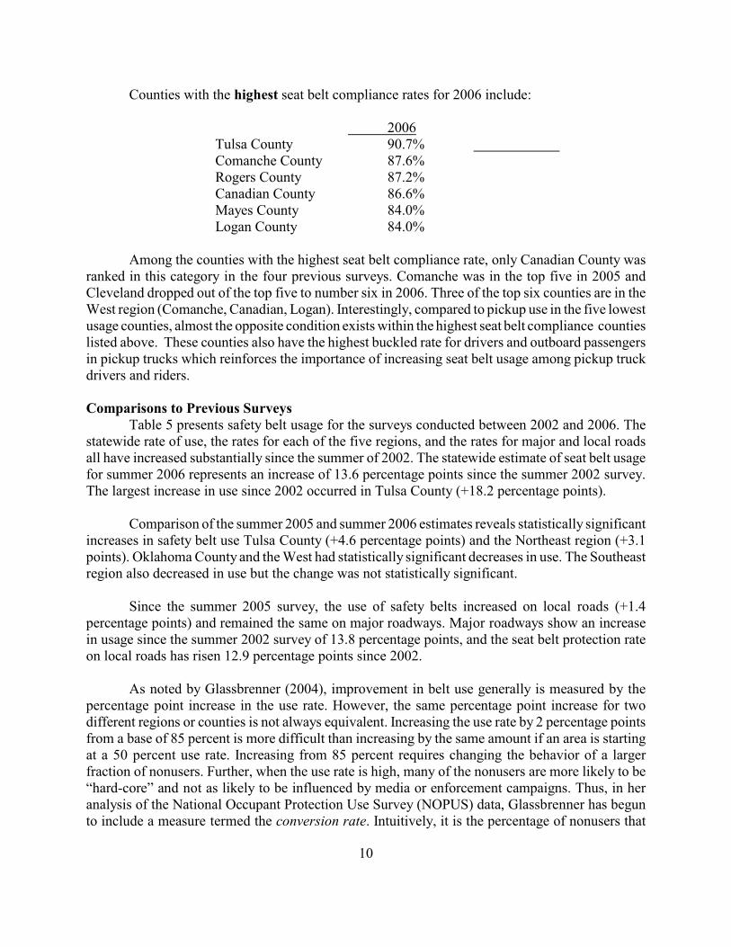
Counties with the highest seat belt compliance rates for 2006 include:
2006Tulsa County 90.7%Comanche County 87.6%Rogers County 87.2%Canadian County 86.6%Mayes County 84.0%Logan County 84.0%
Among the counties with the highest seat belt compliance rate, only Canadian County wasranked in this category in the four previous surveys. Comanche was in the top five in 2005 andCleveland dropped out of the top five to number six in 2006. Three of the top six counties are in theWest region (Comanche, Canadian, Logan). Interestingly, compared to pickup use in the five lowestusage counties, almost the opposite condition exists within the highest seat belt compliance countieslisted above. These counties also have the highest buckled rate for drivers and outboard passengersin pickup trucks which reinforces the importance of increasing seat belt usage among pickup truckdrivers and riders.
Comparisons to Previous SurveysTable 5 presents safety belt usage for the surveys conducted between 2002 and 2006. The
statewide rate of use, the rates for each of the five regions, and the rates for major and local roadsall have increased substantially since the summer of 2002. The statewide estimate of seat belt usagefor summer 2006 represents an increase of 13.6 percentage points since the summer 2002 survey.The largest increase in use since 2002 occurred in Tulsa County (+18.2 percentage points).
Comparison of the summer 2005 and summer 2006 estimates reveals statistically significantincreases in safety belt use Tulsa County (+4.6 percentage points) and the Northeast region (+3.1points). Oklahoma County and the West had statistically significant decreases in use. The Southeastregion also decreased in use but the change was not statistically significant.
Since the summer 2005 survey, the use of safety belts increased on local roads (+1.4percentage points) and remained the same on major roadways. Major roadways show an increasein usage since the summer 2002 survey of 13.8 percentage points, and the seat belt protection rateon local roads has risen 12.9 percentage points since 2002.
As noted by Glassbrenner (2004), improvement in belt use generally is measured by thepercentage point increase in the use rate. However, the same percentage point increase for twodifferent regions or counties is not always equivalent. Increasing the use rate by 2 percentage pointsfrom a base of 85 percent is more difficult than increasing by the same amount if an area is startingat a 50 percent use rate. Increasing from 85 percent requires changing the behavior of a largerfraction of nonusers. Further, when the use rate is high, many of the nonusers are more likely to be“hard-core” and not as likely to be influenced by media or enforcement campaigns. Thus, in heranalysis of the National Occupant Protection Use Survey (NOPUS) data, Glassbrenner has begunto include a measure termed the conversion rate. Intuitively, it is the percentage of nonusers that

11
were converted to users. Since the data generated by the seat belt use surveys are snapshots of use,interpreting the reduction in nonuse as the percentage of nonusers that were converted to users isnot strictly correct. No data are available to document the degree of use (e.g., all the time, half thetime, etc.). However, the general interpretation provides an intuitive means to assess improvementsin belt use.
Table 5Comparison of Seat Belt Use in Oklahoma:
2002-2006(Weighted Percent)
Sum‘02
Sum‘03
Sum ‘04
Sum ‘05
Sum‘06
PercentagePoint
Change‘05-‘06
ConversionRate*
‘05-‘06
Statewide 70.1 76.7 80.3 83.1 83.7 +0.6** 3.7
Regions (non-metro)
West 66.1 72.9 83.5 86.7 83.6 -3.1** -23.3
Northeast 67.8 77.5 76.6 76.9 80.0 +3.1** 13.4
Southeast 68.2 70.9 75.2 81.0 79.9 -1.1 -5.8
Metropolitan Counties
Oklahoma 76.4 76.2 81.2 82.8 81.3 -1.5** -8.7
Tulsa 72.5 88.1 82.7 86.1 90.7 +4.6** 33.1
Roadway Type
Major 69.7 76.6 79.2 83.5 83.5 0.0 0.0
Local 70.6 76.8 81.1 82.1 83.5 +1.4** 7.8
*The conversion rate is the percentage reduction in belt nonuse. It is the percentage point change from 2005 to 2006
divided by the percentage on nonusers in 2005. A negative number is the percentage increase in nonusers.
**Differences are statistically significant at the .05 level using a difference of proportions test.
Table 5 includes a column that provides the conversion rate for increases in use between the2005 and 2006 summer surveys. Statewide the 0.6 percentage point increase from last year isequivalent to a 3.6 percent decrease in nonusers. The largest percentage reduction in nonusersoccurred in Tulsa County (33.1 percent); the Northeast region experienced a 13.4 percent reduction.

12
Between the observation periods from 2002 and 2006, belt nonuse statewide was reduced by 45.5percent. The greatest decrease in nonuse took place in the Tulsa County (66.2 percent), followed bythe West (51.2 percent), the Northeast (37.9 percent), the Southeast (36.8 percent), and OklahomaCounty (20.8 percent).
Use by Gender and RaceTable 6 presents the differences in unweighted belt usage by gender and race. Overall,
females (86.8 percent) are more likely to be buckled than males (79.8 percent). The same patternholds when considering the gender of drivers and passengers. The difference is slightly greateramong the passengers. Usage among male passengers was 9.2 percentage points lower than femalepassengers. Among drivers, 6.8 percent fewer males buckled up compared to females. Themale/female results in Oklahoma are consistent with the national trend. Based on the 2005 NOPUSdata, Glassbrenner (2005a) reports that 84 percent of females buckled up compared to 80 percentof the males observed. Further, the pattern of statistically higher use among females has beenevident in the NOPUS data for several years.
Non-white occupants buckled up at a rate of 84.4 percent, while belt usage among whiteswas 82.8 percent. Similarly, non-white drivers were more likely to be buckled than white drivers.Non-white and white passengers buckled at essentially the same rate.
Table 6Estimate of Seat Belt Use in Oklahoma By Gender and Race:
Summer 2006Unweighted Percent
(n size)*
Female Male Non-White White
Drivers 87.0**(13,544)
80.2**(19,662)
84.8**(4,682)
82.7**(28,615)
Passengers 86.5**(5,686)
77.3**(3,199)
83.0(1,265)
83.1(7,755)
All Occupants 86.8**(19,230)
79.8**(22,861)
84.4***(5,947)
82.8***(36,370)
*The total number of observations for the category. For example, of the 13,544 female drivers, 87.0 percent were
buckled. The number of observations by gender or race do not equal the total number of observations (42,761) because
it was not possible to determine the characteristics of some drivers and passengers.
** Statistical significance is calculated within gender and race categories using Chi-square. Differences are statistically
significant at the .0001 level between male and female rates for drivers, passengers, and all occupants, and also for non-
white versus white rates for drivers.
***The difference between non-white and white rates for all occupants is significant at the .02 level.

13
SUMMARY AND RECOMMENDATIONSThis report provides an analysis of a statewide observation study of safety belt use among
42,761 Oklahoma drivers and front-seat outboard passengers conducted in June 2006. The researchdesign used a statewide, multistage, area probability sample of road segments and intersections. Itrepresents a probability sample of all roadways in the state, taking into account regional populationdistributions, metropolitan and non-metropolitan counties, and major and local roadwayclassifications. The total number of sites, 315, was chosen to produce both an accuraterepresentation of counties based on population and satisfactory estimates by region.
The results of the summer 2006 survey can be summarized as follows:
• Statewide safety belt use increased 0.6 of a percentage point, from 83.1 percent in summer2005 to 83.7 percent in summer 2006.
• Although the overall state usage rate increased, only Tulsa County and the Northeast regionbettered their buckled rate between the summer 2005 and summer 2006 surveys; rates inOklahoma County and the Southeast and West regions decreased.
• Tulsa County had the highest overall usage rate in 2006 (90.7 percent); the lowest rateoccurred in the Southeast region (79.9 percent).
• Between 2005 and 2006, the largest percentage reduction in nonusers occurred in TulsaCounty (33.1 percent) followed by a 13.4 percent reduction in the Northeast region.
• Since the summer 2002 survey, the safety belt usage rate in Oklahoma has increasedsignificantly (70.1 percent to 83.7 percent). Over the same time period, belt usage hasincreased by 18.2 percentage points in Tulsa County, 17.5 points in the West, 12.2percentage points in the Northeast, and an 11.7 points in the Southeast. A somewhat smallincrease of 4.9 percentage points occurred in Oklahoma County.
• Statewide seat belt use in the summer 2006 for automobiles (cars, vans, and SUVs/Jeeps)was 86.4 percent and 75.9 percent for pickup trucks.
• Those observed in Tulsa County had the highest usage rate for pickup trucks (84.5 percent).The lowest usage rate for pickup riders occurred in Delaware County (63.1 percent).
• Overall, drivers and passengers observed on major and local roadways (83.5 percent) wererestrained at the same rate.
• Usage among females exceeded the belted rate for males (87.5 percent to 79.8 percent).Overall, 84.4 percent of non-whites were buckled compared to 82.8 percent of whites.
Two factors that have been demonstrated to play key roles in determining a state’s use rateare the nature of the state’s seat belt law and media campaigns conducted to raise use. The 2005

14
NHTSA survey found that those states with stronger belt enforcement laws (primary enforcement)continue to exhibit generally higher buckled rates than states with weaker laws (secondaryenforcement) (Glassbrenner, 2005b). With respect to public education, the main theme of thenational advertising campaign promoted by NHTSA was “Click It or Ticket.” It conveyed amessage that it is illegal not to use safety belts, law enforcement officers are looking for nonuse, andoffenders will be ticketed. The campaign is viewed as a success with safety belt use increasescoincident with the advertising campaign (Solomon, et al., 2003).
Oklahoma has a positive environment with respect to both of these factors. The increase inOklahoma's seat belt usage rate to a level that approaches the national average coincides with achange in policy, as well as recent media campaigns focusing on enforcement of the state’s seat beltlaw. In 1997, House Bill 1443 was passed, which permitted primary enforcement of Oklahoma’ssafety belt use law. A second contributing factor is the aggressive media campaign launched inOklahoma as part of NHTSA’s “Click It or Ticket!” seat belt mobilization drive. Advertisementsand local news coverage emphasized to the public that Oklahoma law enforcement agencies were“buckling down on seat belt violators.”
In light of the data collected as part of the 2006 study, we offer the followingrecommendations:
• Continue to encourage law enforcement agencies to vigorously enforce the OklahomaMandatory Seat Belt Use Act on a consistent basis;
• Continue to pursue a multimedia strategy for educating the public about the benefits of usingseat belts and the consequences of non-compliance with the state seat belt law;
• Enhanced enforcement and education efforts should be directed toward pickup truck driversand passengers, especially men. Targeting specific counties and regions with low usage rates(i.e., the Northeast and Southeast regions) also would likely have a positive impact on ratesin those areas; and
• Begin to collect county-level data on enforcement of the use of seat belts to document therelationship between enforcement efforts and safety restraint use.

15
ENDNOTES
1. For the period from 1991-92 through 1998, the survey included 360 sites in 22 countiesrandomly chosen from the universe of all state counties, including the two certainty counties(Oklahoma and Tulsa Counties). Guidelines from the National Highway Traffic SafetyAdministration (NHTSA) require a design in which at least 85 percent of the state'spopulation is eligible for inclusion in the sample. In an effort to make the Oklahoma surveyas comparable as possible with similar surveys in other states, we eliminated three countiesincluded in previous surveys – Atoka, Cotton, and Greer. These three counties had thesmallest populations among the previously used group of 22. In dropping these threecounties, the sample easily meets the 85 percent population criterion with the remaining totalof 19 counties. In addition, a weighting procedure based on countywide observation data wasdeveloped in consultation with Dr. Dennis Utter of NHTSA. The purpose was to moreaccurately reflect the percentage of belted drivers and passengers and to provide for thecalculation of more precise confidence intervals.
2. A difference of proportions test is used to determine whether or not the difference betweentwo proportions from independent samples are statistically significant. If the differencebetween two proportions is statistically significant, there is a small probability (less than 5in 100) that the difference is due to chance.

16
REFERENCES
Glassbrenner, Donna. 2004. Safety Belt Use in 2004 – Use Rates in the States and Territories(DOT 809 813). Department of Transportation, National Highway Traffic SafetyAdministration, National Center for Statistics and Analysis. Washington, D.C. November.
Glassbrenner, Donna. 2005a. Safety Belt Use in 2005 – Demographic Results (DOT HS 809 969). Department of Transportation, National Highway Traffic Safety Administration,National Center for Statistics and Analysis. Washington, D.C. December.
___________. 2005b. Safety Belt Use in 2005–Use Rates in the States and Territories (DOT HS 809970). Department of Transportation, National Highway Traffic Safety Administration,National Center for Statistics and Analysis. Washington, D.C. November.
Solomon, M.G., Chaudhary, N.K., and Cosgrove, L.A. 2003. Click It or Ticket Safety BeltMobilization Evaluation. Department of Transportation, National Highway Traffic SafetyAdministration, National Center for Statistics and Analysis. Washington, D.C. May.

17
APPENDIX ASeatbelt Observation Sites – June 2006
WEST Region
Canadian County
Local
1. W. Main St. (SH66) @ S. Ranchwood Blvd. (SH 4)
2. N. Mustang Rd. @ Vandamart Ave.
3. N 63 St. @ Banner Rd. rd
4. Elm St. @ Choctaw
5. Banner Rd. @ S. 29 St. th
6. Country Club Rd. @ Elm St.
Major
7. I-40 B @ Country Club Rd.
8. SH 152 @ US 81
9. SH 66 @ JCT Kilpatrick Turnpike
10. SH 4 (Mustang Rd.) @ 29 St. th
11. I-40 @ Morgan Rd.
12. I-40 @ JCT US 281 Spur
13. I-40 @ US 270
14. I-40 @ US 81
15. I-40 @ Banner Rd.
Comanche County
Local
1. NW Cache Rd. @ NW 97 St.th
2. NW 82 St. @ NW Gorend
3. NW 82 St. @ SW Lee Blvd. nd
4. NW 38 St. @ SW Lee Blvd. th
5. NE Gore Blvd. @ SW 45 St.th
6. 90 St. @ SE Lee (SH 7)th
Major
7. SH 49 @ SH 58
8. Indian Trail Rd. (frontage to US 281) @ Mission Rd (1/4 mile S. of US 281/62 JCT)
9. US 281 Bus. (2 St.) @ “C” St. nd
10. US 277 (E/W) @ US 62/US 281 (N/S)
11. US 62 @ Ft. Sill Blvd.
12. US 62/US 281 @ Pine Ave.
13. US 62 @ NW 127 St. th
14. US 62 @ Post Oak Rd.
15. SH 65 @ SH 7
Garfield County
Local
1. Cheyenne St. @ SH 132
2. Imo (3 mi. E of SH 132) @ Drummond Road
3. Chestnut Road @ Cleveland Road
4. Oakwood Road @ Willow
5. 66 Street @ Breckenridge Rd (Purdue St.)th
6. Market Ave. @ 66 St.th

18
Garfield County (continued)
Major
7. US 64 Bus.(Grand Blvd.) @ Willow Road
8. SH 164 @ SH 74
9. SH 412 (SH 60) @ South Adams
10. US 81 @ Southgate Rd
11. SH 74 @ Unnamed Local Rd. (3 mi S of SH 74/164)
12. US 81 @ Drummond
13. US 60 @ Cleveland
14. US 412 (US 64 Bus.) @ Market
15. US 60 (US 412) @ Mill Run (.25 mi. E of Garland Rd.)
Grady County
Local
1. Georgia Ave @ US 277/ US 81 (4 Ave.)th
2. 6 St. @ SH 92 (Grand Terrace Ave.) th
3. Alex Hwy (6 mi. N of Alex) @ SH 39
4. 4 St./Main St. @ SH 92 th
5. South Sara Rd. @ Fox Rd.
6. Cimarron Rd. @ SH 37
Major
7. US 62 @ Locust St.
8. US 81 @ SH 37 West
9. US 81 @ Unnamed Local Rd. (2 mi. N of Chickasha city limit)
10. SH 19 @ 6 St. th
11. US 81/US 277 @ SH 19 E (East Ninnekah line)
12. US 62 @ Maple (2.5 mi. W of SH 39 and SH 9/US 277 JCT)
13. US 81 @ Dutton (½ mi. N of Pocasset)
14. US 81 @ access road to Agawam
15. US 62/SH 9 @ Unnamed Local Rd. (2 ½ mi. W of Chickasha city limit or 3 ½ mi. E of Verden city limit)
Logan County
Local
1. Broadway Blvd. @ Charter Oak Rd.
2. Pine Street @ SH 33 (Noble Ave.)
3. Hale Road @ SH 33
4. Waterloo Rd. @ Douglas Blvd.
5. Monroe @ SH 74 (Grand Ave.)
6. Main St. @ SH 74 E
Major
7. US 77 @ Triplett Rd.
8. SH 33 @ Pennsylvania
9. SH 74 F @ Rockwell Ave.
10. I-35 @ Seward Rd (Exit 151)
11. I-35 @ SH 33 (Exit 157)
12. SH 33 @ US 77
13. US 77 @ Industrial Rd.
14. SH 33 @ 14 St.th
15. I-35 @ Waterloo Rd.

19
NORTHEAST Region
Delaware County
Local
1. Broadway @ SH 85 A (Bernice, OK)
2. Unnamed Local Rd. (in Choleta; 2 mi. E of Mayes County Line) @ SH 20
3. Unnamed Local Rd. (2 mi. S of Ottawa Co.)@ SH 10
4. 13 St. @ Main St. (US 59)th
5. Washbourne @ 9 St.th
6. Cherokee St. @ Tulsa Ave (US 412A)
Major
7. 412 A @ Unnamed Local Rd. (approx. .25 mi. N of US 412/412A JCT)
8. US 59/SH 10 @ Unnamed Local Rd. (3 mi. S of SH 116 & SH10/US 59 JCT)
9. SH 85 A @ SH 125
10. US 412 A @ US 412 A South
11. SH 20 @ SH 28 N
12. SH 28 @ Unnamed Local Rd. (approx. 2 mi. E of county line)
13. SH 20 @ SH 10/US 59
14. US 59/SH 10 @ SH 116
15. US 59 @ New Life Ranch Rd.
Mayes County
Local
1. Unnamed Local Rd. (.25 mi. S of US 412 at JCT with US 69) @ Unnamed Local Rd. (3 ½ mi. W of US 69)
2. Chouteau Ave. (US 69) @ Main St.
3. Unnamed Local Rd. (3 mi. W of Locust Grove city limits) @ US 412A
4. Broadway @ Main (US 412A)
5. 9 St. @ Vann St. th
6. Elliott @ Unnamed Local Rd. (½ mi. S of SE 17 St.)th
Major
7. SH 28 @ SH 82 South
8. SH 20/SH 82 @ Tulsa Ave.
9. US 69 @ Unnamed Local Rd.(approx. 4.25 mi. S of US 412 & 2 mi. N of Wagoner County line)
10. SH 412B @ SH 69A
11. US 69A @ US 69
12. US 69 @ Unnamed Local Rd. (approx. 1.25 mi. S of US 412)
13. US 69 @ Unnamed Local Rd. (2 mi. S of SH 28)
14. US 69 @ Unnamed Local Rd. (2 mi. N of SH 20 JCT)
15. US 412 @ Vann St.
Muskogee County
Local
1. Seminole St. @ Sycamore St.
2. Border @ S. 24 St. th
3. S. 24 St. @ Hancockth
4. Smith Ferry Rd. @ Gulick
5. York St.@ Chandler St.
6. Gibson @ York St.

20
Muskogee County (continued)
Major
7. SH 80A @ SH 80
8. SH 10 @ SH 10A (after #8 is completed, take SH10 South to SH100; then, SH100 South to I-40 for site #9)
9. US 62B @ US 62/US 64
10. US 69 @ US 62 East
11. US 62 @ SH 10 South
12. I-40 @ SH 100
13. I-40 @ US 266/SH 2
14. US 64 @ Davis Field (look for Phillips 66)
15. US 69 @ Unnamed Local Rd. (1 mi. N and 2 mi. W of site #14)
Ottawa County
Local
1. 20 St. @ E St. (Miami, OK)th
2. 12 St. @ E St. (Miami, OK)th
3. Shawnee @ Main St. (Peoria,OK)
4. 12 St. @ College (Cardin, OK)th
5. Main @ Broadway (Wyandotte, OK)
6. Unnamed Local Rd. (½ mi. S of US 60) @ SH 10
Major
7. SH 10 @ SH 137
8. SH 25 @ US 59/US 69 (Narcissa, OK)
9. US 69 A (Main St.) @ SH 137 South (Quapaw, OK)
10. US 60 @ US 60B
11. US 59 @ 20 St. th
12. SH 10 @ Unnamed Local Rd. (2 mi. W of SH 137)
13. US 60 @ US 60 B (Seneca, OK)
14. US 60 (Conner Ave.) @ Cherry St. (Fairland, OK)
15. US 69 @ Veterans Blvd. (Miami, OK)
Payne County
Local
1. W 19 Ave. @ Sangreth
2. Western @ W. 32 St. nd
3. US 177 (Main St.) @ Thomas Ave.
4. Fairgrounds Rd. @ Mahen Rd.
5. Lakeview @ N. Country Club Rd.
6. Coyle Rd. @ SH 51
Major
7. SH 33 @ Harmony Rd.
8. SH 33 @ Logan County Line (128 )th
9. SH 18 @ SH 33 (prior to fork)
10. SH 51 @ Redland Rd.
11. SH 51 @ Washington
12. SH 18/SH 33 @ Brethren Rd.
13. SH 18 (North to Little Axe) @ SH 18/SH 33 (Main St.)
14. US 177 @ SH 33
15. I-35 @ SH 51

21
Rogers County
Local
1. 106 St. @ 161 East Ave. th st
2. 145 St. @ 96 St.th th
3. Vera Rd. (EW 39) @ Maple St. (NS 408)
4. Unnamed Local Rd./EW 39 (approx. 3.75 mi. W of US 169) @ Unnamed Local Rd./NS 406 (1 mi. N of Vera)
5. Pine St. @ E 161 Ave.st
6. Cherokee St. @ Pine St.
Major
7. SH 66 @ SH 88 (1 St.)st
8. US 169 @ Tulsa County line
9. SH 66 @ SH 28 A
10. US 169 (Elm) @ Delaware St.
11. SH 266 @ SH 167
12. SH 66 @ Unnamed Local Rd./EW 45 (4 ½ mi. N of SH 20 or 6 mi. S of SH 28 A)
13. US 412 @ SH 88
14. US 412 @ Unnamed Local Rd./Crossroads NS 416 (6 mi. E of SH 167)
15. US 412/I-44 @ SH 167
SOUTHEAST Region
Bryan County
Local
1. Unnamed Local Rd. @ SH 78
2. Unnamed Local Rd. @ SH 78 (Ury)
3. Hillcrest Drive @ McLean
4. Mulberry St.@ First St.
5. Franklin @ Snider
6. Franklin @ Smiser (6 mi. N of SH 91)
Major
7. US 70 @ 7 St. NWth
8. SH 78 @ SH 70 E
9. SH 78 (SE. 3 St.) @ Georgia St. (1 mi. S of Mulberry St.)rd
10. US 69 Bus./US 75 Bus. @ Rodeo
11. US 70 @ Unnamed Local Rd. (2 ½ mi. W of Walnut in Mead)
12. US 70 @ Unnamed Local Rd. (½ mi. E of Walnut)
13. US 69 @ SH 91
14. US 69 @ McKinley (SE corner of Calera)
15. US 69/US 75 @ Armstrong Exit
Carter County
Local
1. W Lake Rd. @ 8 St. (SH 76) th
2. Texas Road @ 1 St. st
3. Prairie Valley Rd. @ Lake Ardmore Rd.
4. Hedges Rd. @ Unnamed Local Rd. (approx. 1.75 mi. S of US 70 & I-35 JCT)
5. Monroe Ave. @ Mt. Washington Rd.
6. Veterans Blvd. (SH 142) @ Refinery Road
Major
7. SH 76 @ SH 7 (E. Main St.)
8. SH 199 (Sam Noble Parkway) @ Gene Autry Rd.

22
Carter County (continued)
Major (continued)
9. US 70 @ SH 77 South (S. Lake Murray Dr.)
10. US 70 @ SH 77 South
11. I-35 @ 12 Ave. NWth
12. SH 199 @ US 177
13. I-35 @ SH 53 E
14. I-35 @ SH 77 South
15. I-35 @ SH 53 W
Cleveland County
Local
1. Main St. @ 36 Ave.th
2. 36 Ave. @ Robinsonth
3. 24 Ave. SE @ Rock Creekth
4. Porter Ave. @ Franklin Rd.
5. Slaughterville Rd. @ 120 Ave. SEth
6. 120 Ave., SE @ Spring Hill Rd. (SH 39)th
Major
7. SH 74A (Lindsey St.) @ Jenkins Ave.
8. SH 37 (134 St.) @ Portland Ave. th
9. SH 9 @ 48 Ave. SE th
10. I-35 @ SE 89 St. th
11. I-35 @ N 12 St. th
12. I-35 @ Robinson St.
13. I-35 @ Indian Hills Rd.
14. SH 77 (Flood Ave) @ Tecumseh Rd.
15. I-35 @ 19 St. th
McClain County
Local
1. Walnut Creek Rd. (S. 7th) @ MacArthur Ave.
2. Morehead St. @ Main St.
3. N. Main (SH 74) @ W. Center Rd.
4. Johnson Ave. @ 180 St. th
5. 9 St. @ Grant St. th
6. Barger (US 77) @ Seifried St.
Major
7. SH 9 @ S Santa Fe Ave.
8. US 62 @ NW 24 St. th
9. I-35 @ SH 9 (Exit 106)
10. I-35 @ Purcell (Exit 91)
11. SH 9/ US 62/ US 277 @ MacArthur Ave.
12. I-35 @ Goldsby (Exit 104)
13. SH 74B @ SH 74 (270 St.) th
14. I-35 @ SH 59
15. I-35 @ SH 74
23
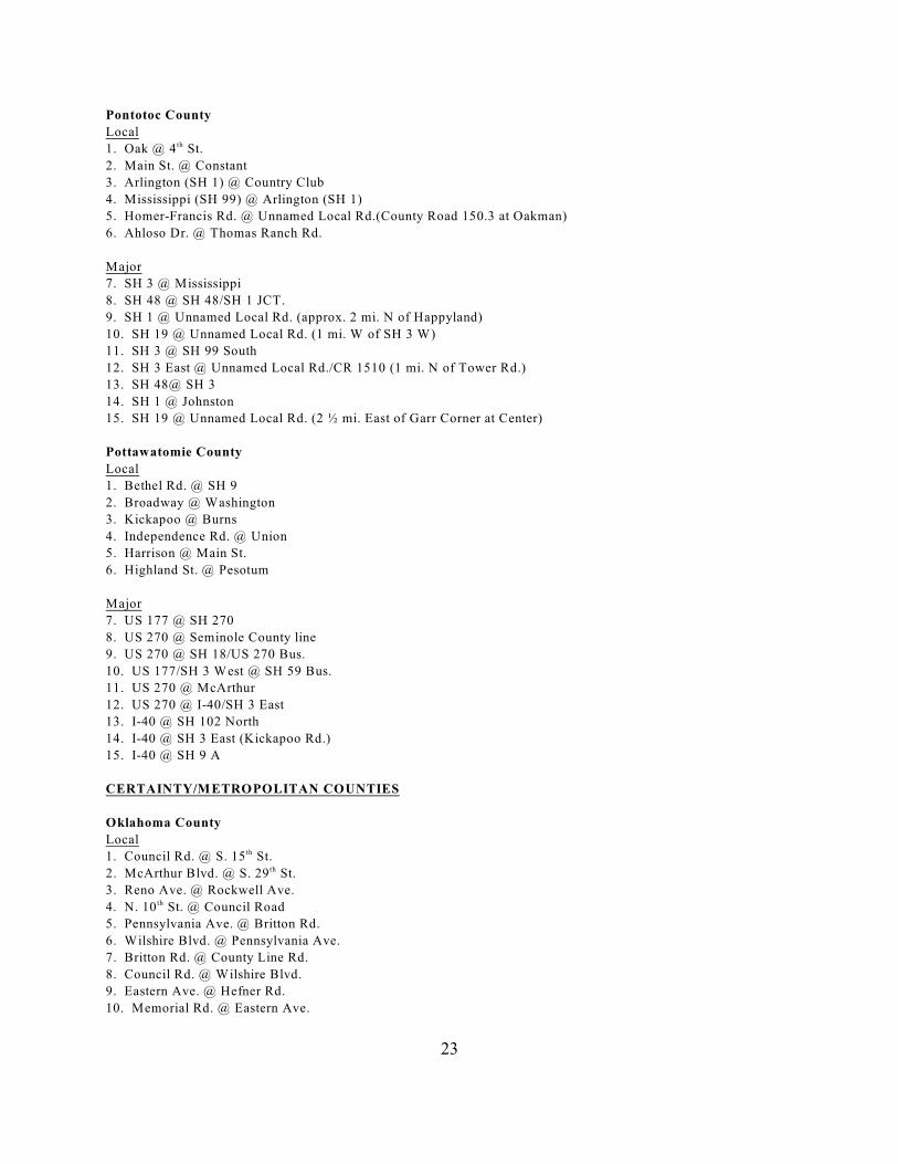
Pontotoc County
Local
1. Oak @ 4 St. th
2. Main St. @ Constant
3. Arlington (SH 1) @ Country Club
4. Mississippi (SH 99) @ Arlington (SH 1)
5. Homer-Francis Rd. @ Unnamed Local Rd.(County Road 150.3 at Oakman)
6. Ahloso Dr. @ Thomas Ranch Rd.
Major
7. SH 3 @ Mississippi
8. SH 48 @ SH 48/SH 1 JCT.
9. SH 1 @ Unnamed Local Rd. (approx. 2 mi. N of Happyland)
10. SH 19 @ Unnamed Local Rd. (1 mi. W of SH 3 W)
11. SH 3 @ SH 99 South
12. SH 3 East @ Unnamed Local Rd./CR 1510 (1 mi. N of Tower Rd.)
13. SH 48@ SH 3
14. SH 1 @ Johnston
15. SH 19 @ Unnamed Local Rd. (2 ½ mi. East of Garr Corner at Center)
Pottawatomie County
Local
1. Bethel Rd. @ SH 9
2. Broadway @ Washington
3. Kickapoo @ Burns
4. Independence Rd. @ Union
5. Harrison @ Main St.
6. Highland St. @ Pesotum
Major
7. US 177 @ SH 270
8. US 270 @ Seminole County line
9. US 270 @ SH 18/US 270 Bus.
10. US 177/SH 3 West @ SH 59 Bus.
11. US 270 @ McArthur
12. US 270 @ I-40/SH 3 East
13. I-40 @ SH 102 North
14. I-40 @ SH 3 East (Kickapoo Rd.)
15. I-40 @ SH 9 A
CERTAINTY/METROPOLITAN COUNTIES
Oklahoma County
Local
1. Council Rd. @ S. 15 St. th
2. McArthur Blvd. @ S. 29 St.th
3. Reno Ave. @ Rockwell Ave.
4. N. 10 St. @ Council Roadth
5. Pennsylvania Ave. @ Britton Rd.
6. Wilshire Blvd. @ Pennsylvania Ave.
7. Britton Rd. @ County Line Rd.
8. Council Rd. @ Wilshire Blvd.
9. Eastern Ave. @ Hefner Rd.
10. Memorial Rd. @ Eastern Ave.

24
Oklahoma County (continued)
Local (continued)
11. S. 15 St. @ Kelley Ave.th
12. Kelley Ave. @ Edmond Rd.
Major
13. I-40 @ Sunnylane Rd.
14. I-240 @ SH 77
15. I-40 @ Douglas Blvd.
16. SH 3 (NW Expressway) @ Wilshire Blvd.
17. I-40 @ Agnew Rd.
18. I-44 @ Eastern/MLK Ave.
19. I-44 @ Pennsylvania Ave.
20. SH 74 (Hefner Parkway) @ Britton Rd.
21. I-35 @ Grand Blvd.
22. I-240 @ Bryant (Exit 6)
23. I-35 @ S.E. 59 St. th
24. US 77 (Broadway Extension) @ Hefner Rd.
25. I-44 @ SW 29 St.th
26. I-235 @ N. 50 St.th
27. SH 74 (Hefner Parkway) @ Hefner Rd.
28. I-44 @ N. 23 St.rd
29. I-40 @ Council Rd.
30. I-35 @ N. 10 St. th
Tulsa County
Local
1. 141 St. South @ US 75 st
2. Peoria Ave. @ 141 St. Southst
3. Elwood Ave. (4 Ave.) @ West 111 St. Southth th
4. West 91 St. South @ Union Ave. st
5. 81 St. (Houston) @ Olive Ave (129 /Mayo Rd.)st th
6. Garnett Rd. @ West 91 St. (Washington St.)st
7. 145 Ave. (Aspen Ave.) @ 11 St.th th
8. 21 St. @ 17 Ave. /Lynn Lane Rd.st th
9. 41 St. @ Lewis (25 Ave.)st th
10. Lewis (24 ) Ave. @ 51 (Omaha) th st
11. 11 St. @ Pittsburghth
12. Yale (49 Ave.) @ 11 St. th th
Major
13. SH 266 (East 46 St. North) @ Mayo Rd. (Olive/129th) th
14. US 64 (Memorial Rd/81st Ave.) @ 41 St.st
15. I-244 @ Memorial Drive (81 Ave.)st
16. SH 11 @ Pine (15 ) St. th
17. I-44 @ 21 St. st
18. US 169 @ 46 St./SH 266 Eastth
19. SH 51 (US 64) @ 65 Ave. (Sheridan Rd.)th
20. US 169 @ SH 20 East (116 St.)th
21. US 75 @ Pine St.
22. US 64 @ 81 West Ave. st
23. US 75 @ E. 86 St. North th
24. I-244 (US 412) @ Mingo Rd. (97 Ave.)th
25. SH 51 (US 64) @ Harvard (33 Ave.)rd

25
Tulsa County (continued)
Major (continued)
26. I-44 @ Harvard (33 Ave.)rd
27. I-244 @ Yale (49 Ave.)th
28. US 169 @ Pine St. (15 St.) th
29. US 169 (Old 64) @ 61 St. (Albany St.)st
30. I-244 (US 412) @ Lewis (24 Ave.)th

26
APPENDIX BESTIMATION AND ANALYSIS PROCEDURES
ESTIMATION OF BELT USAGE Safety belt usage rates were estimated separately for major and local roads within each county.All estimates were generated using SPSS statistical software. The estimates for major roads can beexpressed as
ij1 ij1 ijk1 ijk1 R = 1/n * S (B /O )where
ijk1 B = number of observed belted occupants at road segment;
ijk1O = number of observed occupants at road segment;
ij1n = number of sample units of road segment type.
Estimates of local road usage rates can be expressed as
ij2 ijk1 ijk1R = S B / S O
Estimates of county-wide usage rates can be expressed as
ijm ijm ij1 ij1V * R + V * R
ij ijm ij1R = V + V
where
ijmV = average daily vehicle miles traveled (VMT) for major roads;
ij1V = VMT for local roads.
County-wide sampling weights can be expressed as
ij i i W =P / (P * ni)where
i ijP = total population of region; P = population of county;
ijn = number of counties sampled in region.
27
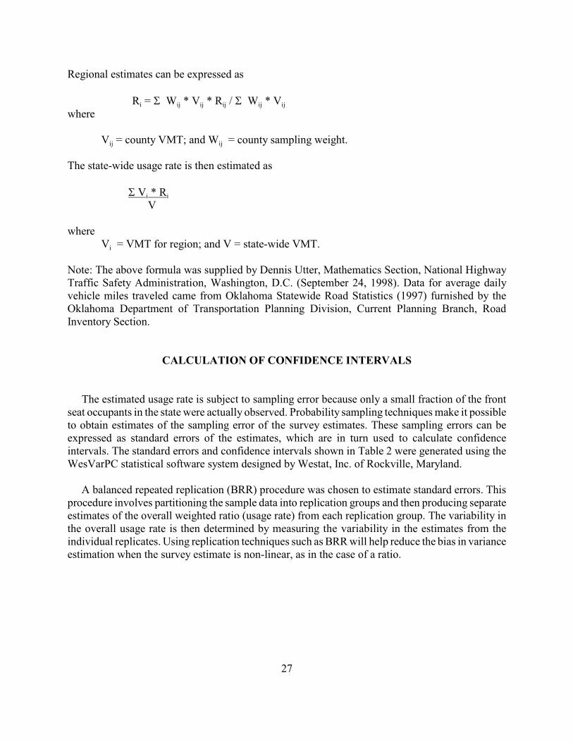
Regional estimates can be expressed as
i ij ij ij ij ij R = S W * V * R / S W * Vwhere
ij ijV = county VMT; and W = county sampling weight.
The state-wide usage rate is then estimated as
i iS V * R V
where
i V = VMT for region; and V = state-wide VMT.
Note: The above formula was supplied by Dennis Utter, Mathematics Section, National HighwayTraffic Safety Administration, Washington, D.C. (September 24, 1998). Data for average dailyvehicle miles traveled came from Oklahoma Statewide Road Statistics (1997) furnished by theOklahoma Department of Transportation Planning Division, Current Planning Branch, RoadInventory Section.
CALCULATION OF CONFIDENCE INTERVALS
The estimated usage rate is subject to sampling error because only a small fraction of the frontseat occupants in the state were actually observed. Probability sampling techniques make it possibleto obtain estimates of the sampling error of the survey estimates. These sampling errors can beexpressed as standard errors of the estimates, which are in turn used to calculate confidenceintervals. The standard errors and confidence intervals shown in Table 2 were generated using theWesVarPC statistical software system designed by Westat, Inc. of Rockville, Maryland.
A balanced repeated replication (BRR) procedure was chosen to estimate standard errors. Thisprocedure involves partitioning the sample data into replication groups and then producing separateestimates of the overall weighted ratio (usage rate) from each replication group. The variability inthe overall usage rate is then determined by measuring the variability in the estimates from theindividual replicates. Using replication techniques such as BRR will help reduce the bias in varianceestimation when the survey estimate is non-linear, as in the case of a ratio.

28
APPENDIX CRANDOM ASSIGNMENT OF OBSERVERS
This appendix outlines the procedure for the random assignment of days, times, and traffic lanes to the 315 survey
sites. Random assignment is done to eliminate observer discretion and to ensure that all days of the week, all daylight
hours, and both directions of traffic flow are eligible for data gathering. We begin by pre-grouping the sites into sets –
sites within one county that an observer could reasonably accomplish in a day. We then randomly assign those groups
of sites to days of the week. Once each set is assigned to a day, the sites in it are randomly assigned to start times
beginning on the hour. The example below illustrates how these random assignments are made.
Step 1. We divided the state into seven areas. These areas are smaller than the three regions that are used for
aggregating data in the final report so that an individual observer can conduct observations at all of the sites in their
respective area within a period of six days. Each region consists of two or three counties. The Northeast area, for
example, consists of Ottawa, Delaware, and Mayes counties.
Step 2: We determined a sequence for the counties. In the Northeast area it makes sense, given the locations of the
sites, to observe Ottawa first, then Delaware and finally Mayes.
Step 3: We determined sequences for the sites within a county. In Ottawa County, sites 4, 9, 3, 7, 12, 1, 2, and 15
form a rough circle and can be covered in one day. The remaining sites were left for the following day. Their
predetermined sequence is 13, 10, 6, 5, 14, 8, and 11.
Step 4: We selected a day of the week to begin the area. Using a six-sided die and a random number chart obtained
from a standard statistics text, we randomly assigned the start day for the Northeast area. This required three rolls of the
die. The first two rolls determined the column and row on the random number chart where we began our search for a
qualifying digit. The third roll gave us our interval of digits to skip as we searched down the column for the first eligible
digit. Digits one through seven were eligible, with one standing for Sunday (the first day of the week) and seven
indicating Saturday.
Step 5: We selected a starting location for Monday in Ottawa County. Rolling the die again we searched the random
number chart systematically for an eligible site number as our start site for that Monday in Ottawa County. Since eight
sites would be observed on this day the digits one through eight were eligible. The first eligible number we landed on
was 8, site number 4 (eighth on our list) was selected as the start site. Given our predetermined sequence, sites 9, 3, 7,
12, 1, 2, and 15 (in that order) were scheduled to follow site 4 that day.
Step 6: We selected a starting time for site 4. In order to ensure that all daylight hours were eligible for observation,
we randomly selected a start time for that day. Eligible start times, given an eight-site day as opposed to a seven-site day,
were 7, 8, 9, and 10 a.m. (For the next day, when only seven sites would be observed, 11 a.m. also is an eligible start
time.) For example, rolling the die as before, our first eligible number was 8. Therefore, the observer would be scheduled
to begin in Ottawa County on Monday at site number 4 at eight o'clock in the morning. Given the predetermined
sequence, the schedule for Monday in Ottawa County would become:
Site 4 at 8:00 a.m.
Site 9 at 9:00 a.m.
Site 3 at 10:00 a.m.
Site 7 at 11:00 a.m.
Site 12 at Noon
Site 1 at 1:00 p.m.
Site 2 at 2:00 p.m.
Site 15 at 3:00 p.m.
29
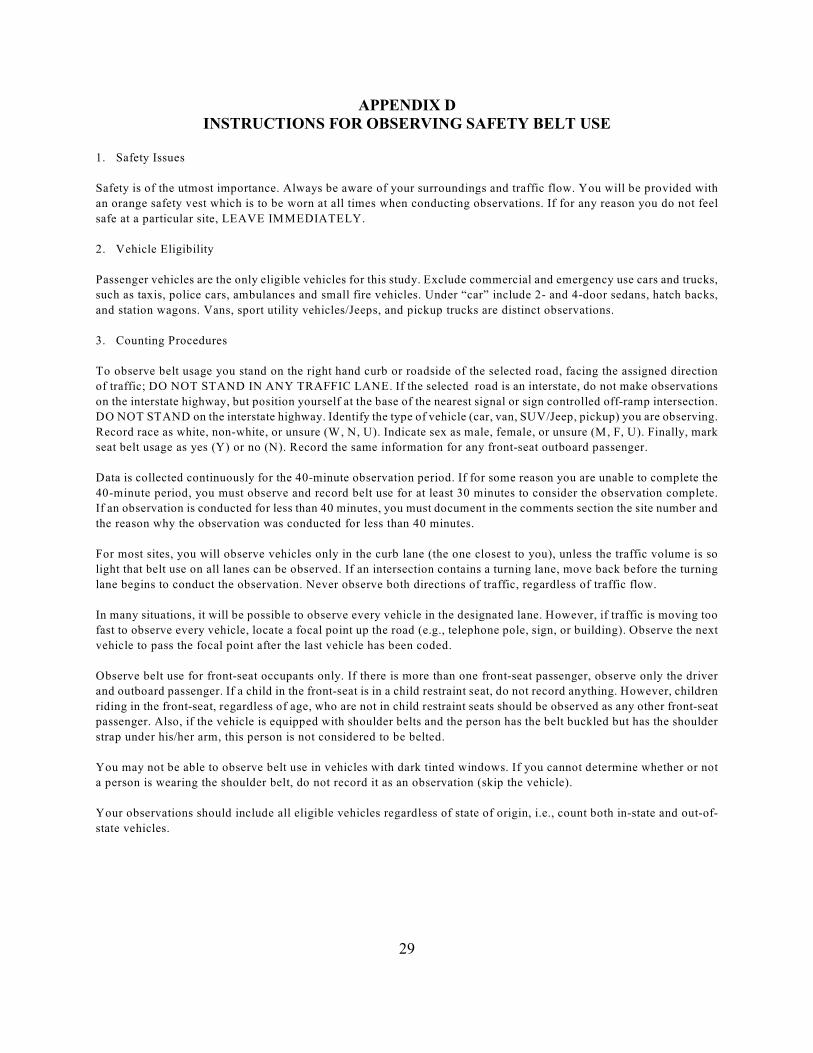
APPENDIX DINSTRUCTIONS FOR OBSERVING SAFETY BELT USE
1. Safety Issues
Safety is of the utmost importance. Always be aware of your surroundings and traffic flow. You will be provided with
an orange safety vest which is to be worn at all times when conducting observations. If for any reason you do not feel
safe at a particular site, LEAVE IMMEDIATELY.
2. Vehicle Eligibility
Passenger vehicles are the only eligible vehicles for this study. Exclude commercial and emergency use cars and trucks,
such as taxis, police cars, ambulances and small fire vehicles. Under “car” include 2- and 4-door sedans, hatch backs,
and station wagons. Vans, sport utility vehicles/Jeeps, and pickup trucks are distinct observations.
3. Counting Procedures
To observe belt usage you stand on the right hand curb or roadside of the selected road, facing the assigned direction
of traffic; DO NOT STAND IN ANY TRAFFIC LANE. If the selected road is an interstate, do not make observations
on the interstate highway, but position yourself at the base of the nearest signal or sign controlled off-ramp intersection.
DO NOT STAND on the interstate highway. Identify the type of vehicle (car, van, SUV/Jeep, pickup) you are observing.
Record race as white, non-white, or unsure (W, N, U). Indicate sex as male, female, or unsure (M, F, U). Finally, mark
seat belt usage as yes (Y) or no (N). Record the same information for any front-seat outboard passenger.
Data is collected continuously for the 40-minute observation period. If for some reason you are unable to complete the
40-minute period, you must observe and record belt use for at least 30 minutes to consider the observation complete.
If an observation is conducted for less than 40 minutes, you must document in the comments section the site number and
the reason why the observation was conducted for less than 40 minutes.
For most sites, you will observe vehicles only in the curb lane (the one closest to you), unless the traffic volume is so
light that belt use on all lanes can be observed. If an intersection contains a turning lane, move back before the turning
lane begins to conduct the observation. Never observe both directions of traffic, regardless of traffic flow.
In many situations, it will be possible to observe every vehicle in the designated lane. However, if traffic is moving too
fast to observe every vehicle, locate a focal point up the road (e.g., telephone pole, sign, or building). Observe the next
vehicle to pass the focal point after the last vehicle has been coded.
Observe belt use for front-seat occupants only. If there is more than one front-seat passenger, observe only the driver
and outboard passenger. If a child in the front-seat is in a child restraint seat, do not record anything. However, children
riding in the front-seat, regardless of age, who are not in child restraint seats should be observed as any other front-seat
passenger. Also, if the vehicle is equipped with shoulder belts and the person has the belt buckled but has the shoulder
strap under his/her arm, this person is not considered to be belted.
You may not be able to observe belt use in vehicles with dark tinted windows. If you cannot determine whether or not
a person is wearing the shoulder belt, do not record it as an observation (skip the vehicle).
Your observations should include all eligible vehicles regardless of state of origin, i.e., count both in-state and out-of-
state vehicles.

(Please use back of sheet to continue your notes if necessary)
APPENDIX E
Oklahoma Safety Belt Observation Form
Observer: __________________________ Location: ___________________________________
Observation Date: __________________ County and Site ID#:__________________________
Start Time (40 min. duration): ________
Corner of Intersection you stood on: _____________
NOTES: _______________________________
Direction of Traffic observed: ___________
DRIVER PASSENGER
VehicleC=CarP=PickupS=SUV/JeepV=Van
RaceW=WhiteN=Non-whiteD=Don’t Know
SexM=MaleF=FemaleD=Don’t Know
UseY=YesN=No
RaceW=WhiteN=Non-whiteD=Don’t Know
SexM=MaleF=FemaleD=Don’t Know
UseY=YesN=No
1
2
3
4
5
6
7
8
9
10
11
12
13
14
15
Summer 2006