Embed Size (px)
Citation preview
Marine Pollution Bulletin 91 (2015) 347–356
Contents lists available at ScienceDirect
Marine Pollution Bulletin
journal homepage: www.elsevier .com/locate /marpolbul
Oil spill contamination probability in the southeastern Levantine basin
http://dx.doi.org/10.1016/j.marpolbul.2014.10.0500025-326X/� 2014 Elsevier Ltd. All rights reserved.
⇑ Corresponding author. Tel.: +972 4 8565246.E-mail addresses: [email protected] (R. Goldman), [email protected] (E. Biton),
[email protected] (E. Brokovich), [email protected] (S. Kark), [email protected] (N. Levin).
Ron Goldman a,⇑, Eli Biton a, Eran Brokovich b, Salit Kark c, Noam Levin b,d
a Israel Oceanographic and Limnological Research, 31080 Haifa, Israelb Department of Geography, The Hebrew University of Jerusalem, Mount Scopus, Jerusalem 91905, Israelc The School of Biological Sciences, ARC Centre of Excellence for Environmental Decisions (CEED), The University of Queensland, Brisbane, Queensland, Australiad School of Geography, Planning and Environmental Management, Centre of Excellence for Environmental Decisions, The University of Queensland, Brisbane, Queensland, Australia
a r t i c l e i n f o
Article history:Available online 18 December 2014
Keywords:SimulationOil spillEastern Mediterranean SeaPollutionProbability
a b s t r a c t
Recent gas discoveries in the eastern Mediterranean Sea led to multiple operations with substantialeconomic interest, and with them there is a risk of oil spills and their potential environmental impacts.To examine the potential spatial distribution of this threat, we created seasonal maps of the probability ofoil spill pollution reaching an area in the Israeli coastal and exclusive economic zones, given knowledge ofits initial sources. We performed simulations of virtual oil spills using realistic atmospheric and oceanicconditions. The resulting maps show dominance of the alongshore northerly current, which causes thehigh probability areas to be stretched parallel to the coast, increasing contamination probability down-stream of source points. The seasonal westerly wind forcing determines how wide the high probabilityareas are, and may also restrict these to a small coastal region near source points. Seasonal variabilityin probability distribution, oil state, and pollution time is also discussed.
� 2014 Elsevier Ltd. All rights reserved.
1. Introduction
The infamous BP/Deepwater Horizon Oil and Gas Disaster in theGulf of Mexico in 2010 (Norse and Amos, 2010) provides a notori-ous example for environmental damages that might result from oiland natural gas exploration and drilling activities. Oil and gasexploration and production have been established in several areasof the Mediterranean Sea for several decades (Belopolsky et al.,2012; Stocker, 2012). Exploration in the Nile Delta has moved fromonshore to offshore areas in the 1980s, and technological advanceshave since enabled exploration and drilling to be used in deepwaters, greatly enhancing the proven reserves of natural gas inthe area. Given the unique biodiversity of the Mediterranean Sea,and the intensity of human activities in the Mediterranean, it ishighly important to better understand the possible impacts of oiland natural gas activities.
As defined in the 1982 UN Convention on the Law of the Sea(UNCLOS), a coastal state has sovereign rights to explore andexploit, conserve and manage the natural resources in its exclusiveeconomic zone (EEZ) (Kwiatkowska, 1991). Under UNCLOS, the EEZcan extend to a maximum distance of 200 nautical miles from thecountry’s baseline.
Following the discoveries of very large gas fields during 2009–2010 in the Israeli EEZ (Fig. 1) there has been an increase in oiland gas exploration and gas production activities (Shaffer, 2011;Ratner, 2011). This increase in offshore exploration and productionactivities brings new challenges to decision makers with regards toconservation efforts, marine safety, and environmental protection.With increased oil and gas operational activity there is also anobvious increase in the risk for oil or other hydrocarbon pollution.Modelling tools enable us to create high resolution probability esti-mates for regions that might be affected by oil pollution. Theresulting probability maps are therefore extremely important todecision makers when forming plans for marine protected areas,placing new infrastructures, or enacting protocols on handlingmarine pollutions.
The use of numerical models to estimate the wind and oceancurrents, which determine oil slick trajectories, has been growingin recent years: Some individual oil spill events that have occurredin the Mediterranean Sea have been simulated (e.g. the Lebanoncrisis oil spill in 2006 (Coppini et al., 2011)) and operationalsystems such as the Mediterranean Decision Support System forMarine Safety (MEDESS-4MS) (Zodiatis et al., 2012) make use ofhigh resolution ocean forecast models to simulate new spills asthey are reported. It is also common to simulate worst case oil spillscenarios for risk assessment.
The aims of this study are: (1) to estimate the location of regionsin Israel’s EEZ that have a high probability of being contaminated byan oil slick. (2) To relate the spatial distribution of these regions to

348 R. Goldman et al. / Marine Pollution Bulletin 91 (2015) 347–356
the initial position of the spill and to the synoptic state (atmosphericand oceanic conditions), so as to improve Israel’s preparedness forthe event of an oil spill. For this end, we produce statistical estimatesof probability based on the simulation of a large number of virtualoil spills which are transported by realistic wind and ocean currents.In that, we follow techniques similar to the ones which have beenused in the gulf of Mexico by OSRA (Price et al., 2003), or in archipel-ago of La Maddalena, located in the northern extremity of SardiniaIsland by Olita et al. (2012). Our work is also related to the workof Ferraro et al. (2009) who used radar based remote sensing ofpossible oil slicks to estimate the density of oil spills in the Mediter-ranean, as well as in other European seas. However, their work wasbased on actual observations which were mapped over a much coar-ser resolution (1�) than the one used in our work.
The manuscript is ordered in the following way: in Section 2 wereview the main characteristics of the regional atmospheric andoceanographic circulations. In Section 3 we briefly describe thenumerical models used in simulating the oil spills and the calcula-tion of oil pollution probabilities. In Section 4 we present and discussthe probability estimates, their seasonality, and their relation to theweather and ocean circulation patterns. We conclude in Section 5.
2. Regional atmospheric and oceanic systems
2.1. Regional meteorology
In our analysis of the results, we consider the following regionalatmospheric and oceanic circulation patterns. The weather in thesouth eastern Mediterranean is characterized by 6 major synopticsystems (Alpert et al., 2004).
1. Cyprus lows – winter low pressure storms whose center travelseast in the northern part of the basin. The winds southeast ofthe center are southerly to easterly winds, whereas strongwesterlies blow west of the cold front.
2. Persian trough is a persistent weather system occurring duringsummer. It is characterized by westerly wind.
3. Red Sea trough (RST also known as Sudan trough) – this troughextends north from the Red Sea during the cold season. The axisof the trough separates the easterly wind east of it from thenortherly wind west of it. The position of this axis, east or westof the coastline, greatly determines the coastal weather.
4. Sharav lows or khamsin lows, which are common in spring, arethermal low pressure systems whose center travels east alongthe southern coast of the Mediterranean. They induce easterlywinds over the sea east of their center and north-westerly windwest of their center.
Fig. 1. Infrastructure in the south eastern corner of the Mediterranean near Israel’sproposed exclusive economic zone. L1: Tamar gas pipeline. L2: Arish–Ashkelonpipeline.
5. Siberian high, is a system which is usually characterized bynortherly winds along the Israeli coast.
6. Subtropical high, is a system which is usually characterized bycalm weather.
2.2. Regional ocean circulation
A major feature in the circulation at the sea surface of thesouth-eastern Mediterranean Sea is a cyclonic along-slope currentflowing over the shelf and slope areas (Rosentraub and Brenner,2007). This current is persistent throughout most of the year,though it may be interrupted by episodes of southward flow. Sug-gested causes of such episodes include strong easterly and north-erly winds typical to the RST, as well as the influence of off-shelfanticyclonic eddies (Rosentraub and Brenner, 2007). The maximalvelocity is usually attained during summer or during storm events(values as high as 1 m/s have been observed during winter(Rosentraub et al., 2010)). The meandering of the along-slope cur-rent has been shown to be related to the exchange of coastal anddeep water in either the detachment of the anticyclonic Shikmonaeddy near Haifa bay (Gertman et al., 2010) or the formation of fil-aments of coastal waters intruding to deep waters (Efrati et al.,2013). Beyond the slope area, the flow is not characterized by a sin-gle permanent feature, but rather by an area populated withdynamic meso-scale eddies (Amitai et al., 2010). The circulationin this area, on average, is anticyclonic, but can be locally inter-rupted by cyclonic mesoscale patterns. Particularly, the areabetween latitudes 33�N and 35�N and east of 32�E, which includesthe Eratostenes sea-mount, is a known location of recurring anticy-clonic eddies (Shikmona/Cyprus eddies). As discussed by Mennaet al. (2012), this area can contain one or two eddies.
3. Methods
In this study we performed numerical simulations of oil spillevents in order to estimate the probability of different areas beingpolluted by oil. We treated different scenarios, each characterizedby the spill event’s proximity to different possible sources of pollu-tion: shipping routes, pipelines, gas wells, single buoy moorings(SBM) and even distribution in space (Fig. 1). From each of thesescenarios, a group of spill events was generated with either ran-dom or even distribution. Ideally, the scenarios should accountfor all the possible synoptic weather and ocean current patternswhich influence the trajectory of the oil slick. In practice, we sam-pled the synoptic conditions by sampling the time of the initialspill from a year of atmospheric and ocean forecasts. Specifically,we used the SKIRON operational atmospheric forecasting systemand the SELIPS circulation forecasts from September 2012 toAugust 2013 to provide wind and currents to the MEDSLIK oil spillmodel. Cutting off in August was motivated by the low variabilityin the atmospheric forcing during this time. We have not consid-ered gas leaks, liquid natural gas spill or gas well blow-outs. Wedid this because the area affected by such events is expected tobe relatively small (e.g., Hightower et al. (2004) recommend a haz-ard radius from liquid natural gas spill to be 2500 m) and the gas isexpected to evaporate and disperse in the atmosphere quickly.
In Sections 3.1 and 3.2 we describe the atmospheric and oceanicmodels used. MEDSLIK is described in Section 3.3. Section 3.4describes how oil spill events were sampled and analysed.
3.1. Atmospheric model – SKIRON
The SKIRON system has been developed by the AtmosphericModeling and Weather Forecasting Group in the university ofAthens (Kallos et al., 1997). SKIRON provides daily atmospheric
R. Goldman et al. / Marine Pollution Bulletin 91 (2015) 347–356 349
forecasts with horizontal spatial resolution of 0.05� and temporalresolution of 1 h. Wind fields of SKIRON are used within the MEDS-LIK oil spill model, whereas fields of wind, air temperature, meansea level pressure, relative humidity, and incoming solar radiationare also used by the ocean circulation model to provide consistentocean currents.
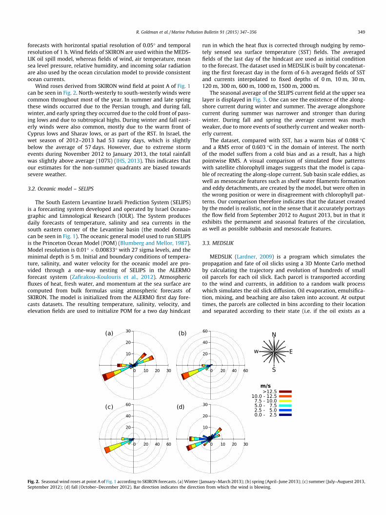
Wind roses derived from SKIRON wind field at point A of Fig. 1can be seen in Fig. 2. North-westerly to south-westerly winds werecommon throughout most of the year. In summer and late springthese winds occurred due to the Persian trough, and during fall,winter, and early spring they occurred due to the cold front of pass-ing lows and due to subtropical highs. During winter and fall east-erly winds were also common, mostly due to the warm front ofCyprus lows and Sharav lows, or as part of the RST. In Israel, thewet season of 2012–2013 had 53 rainy days, which is slightlybelow the average of 57 days. However, due to extreme stormevents during November 2012 to January 2013, the total rainfallwas slightly above average (107%) (IHS, 2013). This indicates thatour estimates for the non-summer quadrants are biased towardssevere weather.
3.2. Oceanic model – SELIPS
The South Eastern Levantine Israeli Prediction System (SELIPS)is a forecasting system developed and operated by Israel Oceano-graphic and Limnological Research (IOLR). The System producesdaily forecasts of temperature, salinity and sea currents in thesouth eastern corner of the Levantine basin (the model domaincan be seen in Fig. 1). The oceanic general model used to run SELIPSis the Princeton Ocean Model (POM) (Blumberg and Mellor, 1987).Model resolution is 0.01� � 0.00833� with 27 sigma levels, and theminimal depth is 5 m. Initial and boundary conditions of tempera-ture, salinity, and water velocity for the oceanic model are pro-vided through a one-way nesting of SELIPS in the ALERMOforecast system (Zafirakou-Koulouris et al., 2012). Atmosphericfluxes of heat, fresh water, and momentum at the sea surface arecomputed from bulk formulas using atmospheric forecasts ofSKIRON. The model is initialized from the ALERMO first day fore-casts datasets. The resulting temperature, salinity, velocity, andelevation fields are used to initialize POM for a two day hindcast
Fig. 2. Seasonal wind roses at point A of Fig. 1 according to SKIRON forecasts. (a) Winter (JSeptember 2012); (d) fall (October–December 2012). Bar direction indicates the directio
run in which the heat flux is corrected through nudging by remo-tely sensed sea surface temperature (SST) fields. The averagedfields of the last day of the hindcast are used as initial conditionto the forecast. The dataset used in MEDSLIK is built by concatenat-ing the first forecast day in the form of 6-h averaged fields of SSTand currents interpolated to fixed depths of 0 m, 10 m, 30 m,120 m, 300 m, 600 m, 1000 m, 1500 m, 2000 m.
The seasonal average of the SELIPS current field at the upper sealayer is displayed in Fig. 3. One can see the existence of the along-shore current during winter and summer. The average alongshorecurrent during summer was narrower and stronger than duringwinter. During fall and spring the average current was muchweaker, due to more events of southerly current and weaker north-erly current.
The dataset, compared with SST, has a warm bias of 0.088 �Cand a RMS error of 0.603 �C in the domain of interest. The northof the model suffers from a cold bias and as a result, has a highpointwise RMS. A visual comparison of simulated flow patternswith satellite chlorophyll images suggests that the model is capa-ble of recreating the along-slope current. Sub basin scale eddies, aswell as mesoscale features such as shelf water filaments formationand eddy detachments, are created by the model, but were often inthe wrong position or were in disagreement with chlorophyll pat-terns. Our comparison therefore indicates that the dataset createdby the model is realistic, not in the sense that it accurately portraysthe flow field from September 2012 to August 2013, but in that itexhibits the permanent and seasonal features of the circulation,as well as possible subbasin and mesoscale features.
3.3. MEDSLIK
MEDSLIK (Lardner, 2009) is a program which simulates thepropagation and fate of oil slicks using a 3D Monte Carlo methodby calculating the trajectory and evolution of hundreds of smalloil parcels for each oil slick. Each parcel is transported accordingto the wind and currents, in addition to a random walk processwhich simulates the oil slick diffusion. Oil evaporation, emulsifica-tion, mixing, and beaching are also taken into account. At outputtimes, the parcels are collected in bins according to their locationand separated according to their state (i.e. if the oil exists as a
anuary–March 2013); (b) spring (April–June 2013); (c) summer (July–Auguest 2013,n from which the wind is blowing.

Fig. 3. Seasonally averaged currents from SELIPS forecasts. (a) Winter (January–March 2013); (b) spring (April–June 2013); (c) summer (July–Auguest 2013, September2012); (d) Fall (October–December 2012).
350 R. Goldman et al. / Marine Pollution Bulletin 91 (2015) 347–356
surface layer, as an emulsion of water and oil within the watercolumn, or if the oil is beached). MEDSLIK has been integrated tothe Mediterranean Decision Support System for Marine Safety(MEDESS-4MS) and is also currently used to assist the Israeli Min-istry of Environmental Protection in case of an oil pollution event.
3.4. Oil spill simulations
Each spill scenario (a group of oil spill releases near pipelines;ship routes; single buoy moorings; gas wells) was simulatedseparately. Conditional probability maps were calculated for eachscenario as described below. In addition, a scenario representinga spatially uniform distribution of oil spills in deep water was alsotreated in order to examine the effects of wind and ocean currentson the conditional probability while mitigating the effect of thelocal initial source distribution. We did not treat scenarios of spillsinside ports or from inland infrastructure. The percentage of oilthat is immediately beached in such events is very sensitive tothe choice of the point were the oil is released. Each spill eventwas simulated separately as an event in which oil is releasedinstantaneously at a specific point and then flows for 10 days.Simulation longer than 10 days resulted in no significant changesto the conditional probability maps. The location of the oil slickwas extracted every 3 h and re-sampled from a grid with bin sizeof 300 m � 300 m to a uniform global grid with bin size of1 km � 1 km. This grid was set in the region south of 33.2�N andeast of 32.5�E. Trimming the domain reduced the problems associ-ated with the boundaries of SELIPS, which include inaccurate cur-rents close to the boundary and the problem of slicks, which leavethe domain but may or may not return to it when currents andwind change direction.
The conditional probability PEðx; yÞ of a bin centered at longi-tude x and latitude y being contaminated, given a spill event inthe scenario E, was estimated as the number of simulations, inthe scenario corresponding to E, in which the bin was contami-nated (at any time point during the 10 day simulation), dividedby the total number of simulations in that scenario. In order to
examine the seasonal changes in conditional probability, we havesubdivided the scenarios according to the date of the initial spills.The date groups are (a) winter: January to March, (b) spring: Aprilto June, (c) summer: July to September and (d) fall: October toDecember. The subscript E, denoting the scenario, is one ofS; P;W;M;U to indicates a source near shipping routes, pipelines,gas wells, single buoy moorings (SBM), or the uniformly distrib-uted grid, respectively.
Formally, if Cðx; y; t;xÞ is the concentration of oil at a bin cen-tered at longitude x and latitude y at time step t ¼ 0 h;3 h;. . . ;240 h resulting from oil spill event x, then a pollution indicatoris defined as:
Iðx; y; T;xÞ ¼1 max Cðx; y; t;xÞ : t < Tf g > 00 otherwise
�; ð1Þ
and conditional probability was estimated as:
PEðx; y; TÞ ¼P
x2EIðx; y; T;xÞPx2E1
: ð2Þ
We denoted PEðx; yÞ ¼: PEðx; y;240 hÞ as the conditional probabilityof being contaminated within 10 day from the initial release.
Mean pollution time was estimated as the average total time inwhich an area is polluted during a simulation:
sðx; yÞ ¼P
x2E
P240 ht¼0 hIðx; y; t;xÞ � 3 hP
x2EIðx; y;240 h;xÞ ð3Þ
The average is taken over simulations in which the bin is pol-luted, thus ‘‘highlighting’’ areas of low conditional probability.The mean time is obviously influenced by the speed of the slick,but also by the shape of the oil slick (e.g. an elliptical slick travelingalong its major axis will produce a longer pollution time than a cir-cular slick having the same area and traveling at the same speed).This analysis is less effective when considering areas where slicksare still traveling through by the end of the simulations. s values insuch areas are biased toward short pollution time compared toupstream areas. In scenarios containing spatially separated sources

R. Goldman et al. / Marine Pollution Bulletin 91 (2015) 347–356 351
(e.g. the pipeline scenario where slicks arrive from Israeli pipelinesand from Egyptian pipelines), s values may have a bimodal distri-bution due to differences in travel time from the different sources.
Oil spill events near pipelines and shipping routes were sam-pled randomly in space and time to better account for the complexspatial structure and to give a better resolution to these importantsource points. The shipping route ensemble had 12000 simulationsand the pipeline ensemble had 3600. The uniform distribution inensemble U had 4896 simulations with a spacing of 0.277�between grid points (Fig. 1) and 5 days intervals between events.This was done since the entire model domain was too large to beevenly sampled by random distribution. Point data (i.e., SBM andgas wells) was also sampled evenly in time (i.e., every 5 days).We have seen in sensitivity tests that the distribution pattern ofthe estimated conditional probability did not change significantlywhen spill volume was changed. We therefore chose not to sampleover different spill volumes but to use a single instantaneous spillvolume of 100 t. Additionally, we have chosen not to sample overdifferent specific gravity values (prescribed to MEDSLIK as Ameri-can Petroleum Institute gravity, or API gravity) and used a singlevalue of API gravity 42, which is the API gravity of light fuel (petro-leum liquids with an API gravity greater than 10 float on water).
4. Results and discussion
The dominance of the along shore current is clearly seen in themaps of the conditional probability estimates (Figs. 4–7). The effectis demonstrated by the fact that areas of high conditional probabil-ity were elongated parallel to the current and are located some-what downstream from their source area (e.g., Figs. 4, 5c, and7c). Additionally, release areas which were oriented along the coastcreated areas with a higher probability than release areas whichwere oriented across it (Figs. 4 and 8). This occurred because oil
Fig. 4. Seasonal conditional probability for contamination of bin ðx; yÞ given a spill releas(a) winter (January–March 2013); (b) spring (April–June 2013); (c) summer (July–Augulocations where beaching occurred. (For interpretation of the references to colour in thi
slicks that are oriented along the coast travelled along similar oroverlapping trajectories, thus increasing their conditional proba-bility estimate, whereas oil slicks released in areas that are ori-ented perpendicularly to the coast travelled in trajectories whichwere parallel to one another. This effect is more apparent whenone examines, for example, the conditional probability from spillsnear pipelines, derived based only on the first day of the simulationi.e., PPðx; y;24 hÞ (Fig. 9): Slicks originating from the Tamar pipeline(L1 in Fig. 1) were scattered almost perpendicularly to the pipelinewhereas slicks originating near the midsection of Arish–Ashkelonpipeline (L2 in Fig. 1) travelled parallel to it. One should note thatthe conditional probability values in Fig. 9 (0.045 maximum) aresmaller than in Fig. 8 (0.2 maximum) since the slick trajectorieswere shorter and did not yet overlap each other.
The conditional probability maps vary with the seasons. Gener-ally, during winter larger areas had non-zero probability than dur-ing summer. This is most evident when regarding the mooringpoints (Fig. 6): in spring and summer the slicks were pushed towardthe coast, most likely by the westerly wind, and only the nearbycoastal area was affected. This did not occur during winter and fall,and therefore a much larger area was at risk, including deep waterand coasts away from the spills. Another feature, which influencedthe conditional probability pattern, was the existence of anti-cyclonic eddy south west of Haifa bay (33.5�E–34.5�E, 32.4�N–33�N) during summer (Fig. 3c). Slicks whose origin lied inside theeddy remained within it, and some of the slicks whose origin wasat the western side of the alongshore current south of the eddy alsoentered the eddy domain and flowed inside it. In this manner, theconditional probability of pollution of the eddy domain increased(Figs. 4c, 8c, and 7c). Because most origin points were located inthe alongshore current, the eddy features have not dominated theconditional probability field except in the case of PUðx; yÞ (Fig. 7c),where most origin points were located away from the coast.
ed at the ship route area based on 10 days of simulation (PSðx; yÞ). Spills start duringest 2013, September 2012); (d) fall (October–December 2012). purple line indicates figure legend, the reader is referred to the web version of this article.)
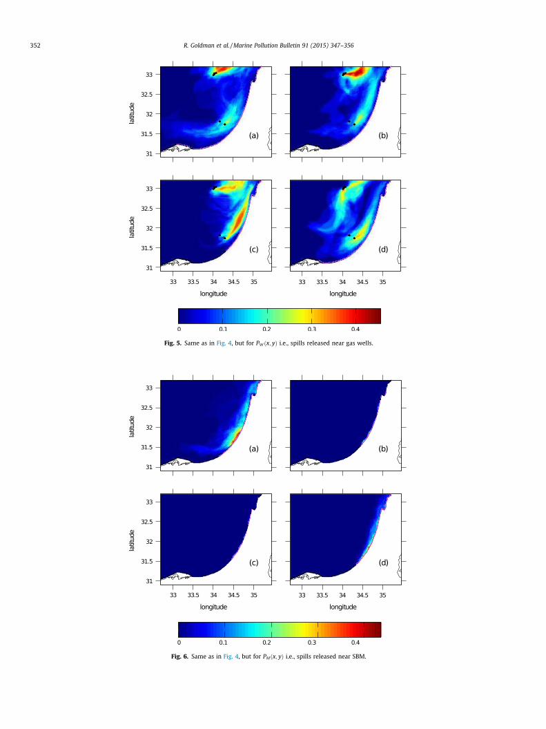
Fig. 5. Same as in Fig. 4, but for PW ðx; yÞ i.e., spills released near gas wells.
Fig. 6. Same as in Fig. 4, but for PMðx; yÞ i.e., spills released near SBM.
352 R. Goldman et al. / Marine Pollution Bulletin 91 (2015) 347–356
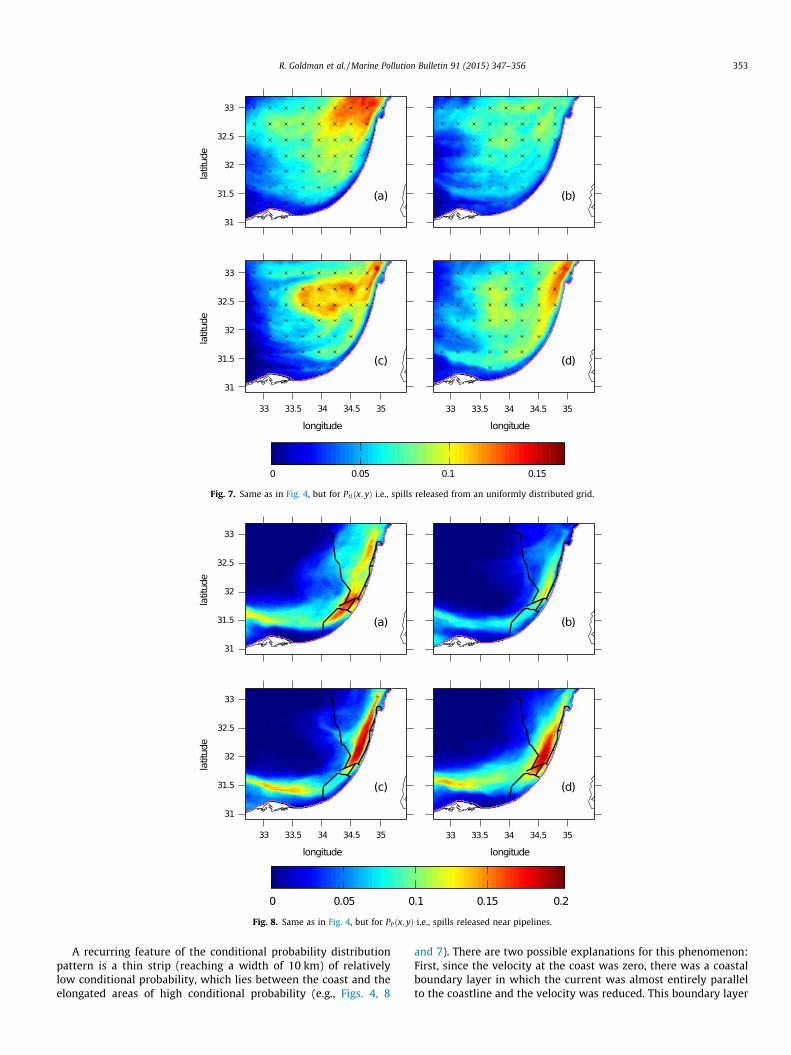
Fig. 7. Same as in Fig. 4, but for PUðx; yÞ i.e., spills released from an uniformly distributed grid.
Fig. 8. Same as in Fig. 4, but for PPðx; yÞ i.e., spills released near pipelines.
R. Goldman et al. / Marine Pollution Bulletin 91 (2015) 347–356 353
A recurring feature of the conditional probability distributionpattern is a thin strip (reaching a width of 10 km) of relativelylow conditional probability, which lies between the coast and theelongated areas of high conditional probability (e.g., Figs. 4, 8
and 7). There are two possible explanations for this phenomenon:First, since the velocity at the coast was zero, there was a coastalboundary layer in which the current was almost entirely parallelto the coastline and the velocity was reduced. This boundary layer
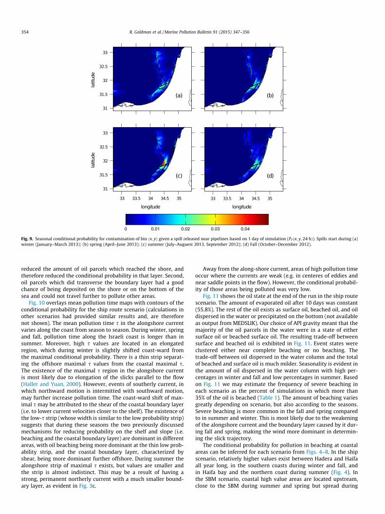
Fig. 9. Seasonal conditional probability for contamination of bin ðx; yÞ given a spill released near pipelines based on 1 day of simulation (PPðx; y;24 hÞ). Spills start during (a)winter (January–March 2013); (b) spring (April–June 2013); (c) summer (July–Auguest 2013, September 2012); (d) Fall (October–December 2012).
354 R. Goldman et al. / Marine Pollution Bulletin 91 (2015) 347–356
reduced the amount of oil parcels which reached the shore, andtherefore reduced the conditional probability in that layer. Second,oil parcels which did transverse the boundary layer had a goodchance of being deposited on the shore or on the bottom of thesea and could not travel further to pollute other areas.
Fig. 10 overlays mean pollution time maps with contours of theconditional probability for the ship route scenario (calculations inother scenarios had provided similar results and, are thereforenot shown). The mean pollution time s in the alongshore currentvaries along the coast from season to season. During winter, springand fall, pollution time along the Israeli coast is longer than insummer. Moreover, high s values are located in an elongatedregion, which during winter is slightly shifted coast-ward fromthe maximal conditional probability. There is a thin strip separat-ing the offshore maximal s values from the coastal maximal s.The existence of the maximal s region in the alongshore currentis most likely due to elongation of the slicks parallel to the flow(Haller and Yuan, 2000). However, events of southerly current, inwhich northward motion is intermitted with southward motion,may further increase pollution time. The coast-ward shift of max-imal s may be attributed to the shear of the coastal boundary layer(i.e. to lower current velocities closer to the shelf). The existence ofthe low-s strip (whose width is similar to the low probability strip)suggests that during these seasons the two previously discussedmechanisms for reducing probability on the shelf and slope (i.e.beaching and the coastal boundary layer) are dominant in differentareas, with oil beaching being more dominant at the thin low prob-ability strip, and the coastal boundary layer, characterized byshear, being more dominant further offshore. During summer thealongshore strip of maximal s exists, but values are smaller andthe strip is almost indistinct. This may be a result of having astrong, permanent northerly current with a much smaller bound-ary layer, as evident in Fig. 3c.
Away from the along-shore current, areas of high pollution timeoccur where the currents are weak (e.g. in centeres of eddies andnear saddle points in the flow). However, the conditional probabil-ity of those areas being polluted was very low.
Fig. 11 shows the oil state at the end of the run in the ship routescenario. The amount of evaporated oil after 10 days was constant(55.8%). The rest of the oil exists as surface oil, beached oil, and oildispersed in the water or precipitated on the bottom (not availableas output from MEDSLIK). Our choice of API gravity meant that themajority of the oil parcels in the water were in a state of eithersurface oil or beached surface oil. The resulting trade-off betweensurface and beached oil is exhibited in Fig. 11. Event states wereclustered either near complete beaching or no beaching. Thetrade-off between oil dispersed in the water column and the totalof beached and surface oil is much milder. Seasonality is evident inthe amount of oil dispersed in the water column with high per-centages in winter and fall and low percentages in summer. Basedon Fig. 11 we may estimate the frequency of severe beaching ineach scenario as the percent of simulations in which more than35% of the oil is beached (Table 1). The amount of beaching variesgreatly depending on scenario, but also according to the seasons.Severe beaching is more common in the fall and spring comparedto in summer and winter. This is most likely due to the weakeningof the alongshore current and the boundary layer caused by it dur-ing fall and spring, making the wind more dominant in determin-ing the slick trajectory.
The conditional probability for pollution in beaching at coastalareas can be inferred for each scenario from Figs. 4–8. In the shipscenario, relatively higher values exist between Hadera and Haifaall year long, in the southern coasts during winter and fall, andin Haifa bay and the northern coast during summer (Fig. 4). Inthe SBM scenario, coastal high value areas are located upstream,close to the SBM during summer and spring but spread during

Fig. 10. Mean pollution time s for the ship route scenario. Contours of conditional probability PS ¼ 0:2 and PS ¼ 0:4 are given for reference. Spills start during (a) winter(January–March 2013); (b) spring (April–June 2013); (c) summer (July–Auguest 2013, September 2012); (d) Fall (October–December 2012).
Fig. 11. Oil state in the entire oil slick after 10 days. Each dot represents an oil spillevent from the ship route scenario.
Table 1Percentage of simulations where more than 35% of the oil is beached.
Scenario Winter Spring Summer Fall
Ship routes 66 75 63 79Even grid 22 30 28 34Gas wells 23 35 37 35SBM 95 100 100 100Pipelines 56 70 66 73
R. Goldman et al. / Marine Pollution Bulletin 91 (2015) 347–356 355
winter and fall (Fig. 6). The pipeline scenario has high values alongthe entire Israeli coast, with a local minima south of Hadera andnorth of Haifa bay (Fig. 8). The evenly distributed grid scenario
has relatively even distribution on the coast, with a slightmaximum between Hadera and Haifa. The gas well scenario hashigher values between Ashdod and Haifa during summer andsouth of Tel-Aviv during winter and fall (Fig. 5).
5. Conclusions
In this study we performed numerical simulations of oil spillevents in Israel’s Mediterranean Sea region, in order to estimatethe conditional probability of different areas being polluted byoil, given that the origin of the spill is close to shipping routes,pipelines, gas wells and single buoy moorings. The simulationswere carried out using the MEDSLIK oil spill model with realisticsynoptic conditions, by sampling the time of the initial spill fromone year of atmospheric and ocean forecasts. Our results exhibitedthe strong influence of circulation patterns (in particular the along-shore current) and seasonality on probability estimates.
Systematic conservation planning involves the definition ofquantitative goals for conserving biodiversity features (e.g., areasrequired for ensuring the persistence of a specific species or habi-tat), and the identification of priority areas that succeed in maxi-mizing the achievement of conservation goals while minimizingthreats or costs (Margules et al., 2002). The outputs of the simula-tions developed in this study can inform the process of systematicconservation planning. Oil spill contamination probabilities can beincorporated as a risk to certain species, depending on their distri-bution range area. Threats to biodiversity can be explicitly includedwithin a prioritization software (Game et al., 2008) as can be doneusing a modified version of the Marxan systematic reserve plan-ning software, called Marxan with Probability (MarProb) (Tullochet al., 2013), with the aim of creating marine protected areas wherethe risks are lower.
356 R. Goldman et al. / Marine Pollution Bulletin 91 (2015) 347–356
Future studies may use more realistic scenarios. Improvementsinclude better mapping of ship routes (see Halpern et al. (2008)and Wang et al. (2008) regarding spatial datasets of shipping tracksand their limitations); considering offshore platforms and shippingin the upstream area of the Nile Delta; accounting for spill size andtype; applying threshold values to concentrations appearing in (1);using more than one year of weather and ocean circulations to getbetter statistics of the synoptic states; and considering events ofnon instantaneous spills near wells, pipes and SBM. Estimatingthe probability of scenario occurrence is also of great importance,especially in cases where one is interested in the probability ofan area being contaminated by oil but not in the source of thepollution.
Acknowledgements
The authors thank the participants of the 2nd internationalworkshop on ‘‘Advancing conservation planning in the Mediterra-nean Sea’’, which took place in Nahsholim Israel (2013), for thefruitful discussions. SK is an Australian Research Council FutureFellow. The authors wish to thank the anonymous reviewer forhis useful suggestions for improving this paper.
References
Alpert, P., Osetinsky, I., Ziv, B., Shafir, H., 2004. Semi-objective classification for dailysynoptic systems: application to the eastern Mediterranean climate change. Int.J. Climatol. 24, 1001–1011. http://dx.doi.org/10.1002/joc.1036.
Amitai, Y., Lehahn, Y., Lazar, A., Heifetz, E., 2010. Surface circulation of the easternMediterranean Levantine basin: insights from analyzing 14 years of satellitealtimetry data. J. Geophys. Res. Oceans, 115. http://dx.doi.org/10.1029/2010JC006147.
Belopolsky, A., Tari, G., Craig, J., Iliffe, J., 2012. New and emerging plays in theeastern Mediterranean: an introduction. Pet. Geosci. 18, 371–372. http://dx.doi.org/10.1144/petgeo2011-096.
Blumberg, A.F., Mellor, G.L., 1987. A description of a three-dimensional coastalocean circulation model. Am. Geophys. Union, 1–16. http://dx.doi.org/10.1029/CO004p0001.
Coppini, G., Dominicis, M.D., Zodiatis, G., Lardner, R., Pinardi, N., Santoleri, R.,Colella, S., Bignami, F., Hayes, D.R., Soloviev, D., Georgiou, G., Kallos, G., 2011.Hindcast of oil-spill pollution during the Lebanon crisis in the easternMediterranean, July–August 2006. Mar. Pollut. Bull. 62, 140–153. http://dx.doi.org/10.1016/j.marpolbul.2010.08.021.
Efrati, S., Lehahn, Y., Rahav, E., Kress, N., Herut, B., Gertman, I., Goldman, R., Ozer, T.,Lazar, M., Heifetz, E., 2013. Intrusion of coastal waters into the pelagic easternMediterranean: in situ and satellite-based characterization. Biogeosciences 10,3349–3357. http://dx.doi.org/10.5194/bg-10-3349-2013.
Ferraro, G., Meyer Roux, S., Muellenhoff, O., Pavliha, M., Svetak, J., Tarchi, D.,Topouzelis, K., 2009. Long term monitoring of oil spills in European seas. Int. J.Remote Sens. 30, 627–645. http://dx.doi.org/10.1080/01431160802339464.
Game, E.T., Watts, M.E., Wooldridge, S., Possingham, H.P., 2008. Planning forpersistence in marine reserves: a question of catastrophic importance. Ecol.Appl. 18, 670–680.
Gertman, I., Goldman, R., Rosentraub, Z., Ozer, T., Zodiatis, G., Hayes, D.R., Poulain,P.M., 2010. Generation Shikmona anticyclonic eddy from long shore current. In:Rapp. Comm. Int. Mer Medit., p. 114.
Haller, G., Yuan, G., 2000. Lagrangian coherent structures and mixing in two-dimensional turbulence. Physica D 147, 352–370. http://dx.doi.org/10.1016/S0167-2789(00)00142-1.
Halpern, B.S., Walbridge, S., Selkoe, K.A., Kappel, C.V., Micheli, F., D’Agrosa, C., Bruno,J.F., Casey, K.S., Ebert, C., Fox, H.E., Fujita, R., Heinemann, D., Lenihan, H.S.,Madin, E.M.P., Perry, M.T., Selig, E.R., Spalding, M., Steneck, R., Watson, R., 2008.A global map of human impact on marine ecosystems. Science 319, 948–952.http://dx.doi.org/10.1126/science.1149345.
Hightower, M., Gritzo, L., Luketa-Hanlin, A., Covan, J., Tieszen, S., Wellman, G., Irwin,M., Kaneshige, M., Melof, B., Morrow, C., Ragland, D. 2004. Guidance on RiskAnalysis and Safety Implications of a Large Liquefied Natural Gas (LNG) SpillOver Water. Technical Report. Sandia National Laboratories Albuquerque NM.
IHS, 2013. Summary of the 2012/13 Rain Year, Hydrological Charectaristics.Technical Report. The Governmental Authority for Water and Sewage.Jerusalem, Israel. In Hebrew.
Kallos, G., Nickovic, S., Papadopoulos, A., Jovic, D., Kakaliagou, O., Misirlis, N.,Boukas, L., Mimikou, N., Sakellaridis, G., Papageorgiou, J., 1997. The regionalweather forecasting system SKIRON: an overview. In: Proceedings of theSymposium on Regional Weather Prediction on Parallel ComputerEnvironments, p. 17.
Kwiatkowska, B., 1991. Creeping jurisdiction beyond 200 miles in the light of the1982 law of the sea convention and state practice. Ocean Dev. Int. Law 22, 153–187. http://dx.doi.org/10.1080/00908329109545954.
Lardner, R. 2009. Medslik v. 5.3.1 User Manual. Oceanography center, University ofCyprus.
Margules, C., Pressey, R., Williams, P., 2002. Representing biodiversity: data andprocedures for identifying priority areas for conservation. J. Biosci. 27, 309–326.http://dx.doi.org/10.1007/BF02704962.
Menna, M., Poulain, P.M., Zodiatis, G., Gertman, I., 2012. On the surface circulationof the Levantine sub-basin derived from Lagrangian drifters and satellitealtimetry data. Deep Sea Res. Part I 65, 46–58. http://dx.doi.org/10.1016/j.dsr.2012.02.008.
Norse, E.A., Amos, J., 2010. Impacts, perception, and policy implications of the BP/Deepwater Horizon oil and gas disaster. Environ. Law Rep. 40, 11058–11073.
Olita, A., Cucco, A., Simeone, S., Ribotti, A., Fazioli, L., Sorgente, B., Sorgente, R., 2012.Oil spill hazard and risk assessment for the shorelines of a Mediterraneancoastal archipelago. Ocean Coast. Manage. 57, 44–52. http://dx.doi.org/10.1016/j.ocecoaman.2011.11.006.
Price, J.M., Johnson, W.R., Marshall, C.F., Ji, Z.G., Rainey, G.B., 2003. Overview of theOil Spill Risk Analysis (OSRA) model for environmental impact assessment. SpillSci. Technol. Bull. 8, 529–533. http://dx.doi.org/10.1016/S1353-2561(03)00003-3.
Ratner, M. 2011. Israel’s Offshore Natural Gas Discoveries Enhance Its Economic andEnergy Outlook. Technical Report.
Rosentraub, Z., Anis, A., Goldman, R., 2010. Wintertime cross shelf circulation andshelf/slope interaction off the central israeli coast. In: Rapp. Comm. Int. MerMedit., p. 171.
Rosentraub, Z., Brenner, S., 2007. Circulation over the southeastern continental shelfand slope of the Mediterranean Sea: direct current measurements, winds, andnumerical model simulations. J. Geophys. Res. Oceans, 112. http://dx.doi.org/10.1029/2006JC003775.
Shaffer, B., 2011. Israel-new natural gas producer in the Mediterranean. EnergyPolicy 39, 5379–5387. http://dx.doi.org/10.1016/j.enpol.2011.05.026.
Stocker, J., 2012. No EEZ solution: the politics of oil and gas in the easternMediterranean. Middle East J 66, 579–597.
Tulloch, V.J., Possingham, H.P., Jupiter, S.D., Roelfsema, C., Tulloch, A.I., Klein, C.J.,2013. Incorporating uncertainty associated with habitat data in marine reservedesign. Biol. Conserv. 162, 41–51. http://dx.doi.org/10.1016/j.biocon.2013.03.003.
Wang, C., Corbett, J.J., Firestone, J., 2008. Improving spatial representation of globalship emissions inventories. Environ. Sci. Technol. 42, 193–199. http://dx.doi.org/10.1021/es0700799.
Zafirakou-Koulouris, A., Koutitas, C., Sofianos, S., Mantziafou, A., Tzali, M., Dermissi,S.C., 2012. Oil spill dispersion forecasting with the aid of a 3D simulation model.J. Phys. Sci. Appl. 10, 448–453.
Zodiatis, G., Lardner, R., Solovyov, D., Panayidou, X., De Dominicis, M., 2012.Predictions for oil slicks detected from satellite images using MyOceanforecasting data. Ocean Sci. 8, 1105–1115. http://dx.doi.org/10.5194/os-8-1105-2012.