Embed Size (px)
Citation preview

i Karlstads universitet 651 88 Karlstad
Tfn 054-700 10 00 Fax 054-700 14 60
Faculty of Economic Sciences, Communication and IT
Leyth Al-Ameri
OIL AND THE
MACROECONOMY
Empirical evidence from 10 OECD countries
Economics Master´s Thesis
Semester: Spring 2012
Instructor: Karl-Markus Modén

i
”…Now oil prices and many broader indices of commodity prices are again at or near all-time
highs in nominal terms, and are very high in real terms as well. Copper, platinum, nickel, zinc
and lead, for example, all hit record highs in 2006, in addition to crude oil. As a result,
commodities are once again hot. It turns out that mankind has to live in the physical world
after all!...” Jeffrey Frankel, 2006

ii
Abstract
This paper examines the oil price-macro economy relationship by means of analyzing the impact of
oil price on Industrial production, real effective exchange rate, real long term interest rate and
inflation rate for a sample of ten OECD countries using quarterly data for the period 1970q1-2011q1.
The impact of oil price shock on industrial production is negative and occurs with a lag of one year.
However, the impact has weakened considerably compared to the 1970s. The impact on real
effective exchange rate is negative/positive for a net importer/exporter, and the magnitude of the
shock depends on the county´s share of net import/export of total world demand/supply. Real
interest rates are affected negatively, through increase in inflation rates following the oil price shock.
The effect tends to die out after 5-8 quarters following the shock for most of the variables and
countries. This paper also applies alternative methods to test for unit root and cointegration, which
takes into account for structural breaks in the data. The weakness of Phillips-Peron test is clearly
demonstrated in the case of inflation rates and real interest rates, where the test falsely considered
the series to be non-stationary when they in fact are stationary around a structural break. There is
also strong evidence of cointegration between oil price and inflation rates and between oil price and
real interest rates, especially when taking account for structural breaks.
This study also highlights the relevance of oil scarcity and oil peak theory. It is shown
that these two terms should receive more attention than they have received so far as more oil
exporters have reached their production peaks and more are likely to be followed. Oil scarcity seems
not to be reflected in the price of oil, this in turn will increase the risk for the search for alternatives
being initiated too late. Scarcity could then pose a serious limitation to the economy before a
substitute resource or technology has been found. According to the data, renewable source of
energy are not likely to dominate OECD countries energy mix in the short term, instead, there is a
trend of increasing natural gas consumption among most of OECD countries. Natural gas markets are
likely to play an equal role in the future as oil markets do today. The dilemma that importing
countries are facing today, particularly in Europe, is whether to expose their markets to Russia or to
the Middle East.

Table of contents Chapter 1: Introduction ......................................................................................................................1
Chapter 2: Non-renewable natural resources ......................................................................................5
2.1 The importance of oil for oil-importing OECD countries .............................................................5
2.2 Oil Scarcity ................................................................................................................................9
2.3 Why do oil prices not increase in the long-term? ..................................................................... 11
Chapter 3: Some words on the relationship between oil prices and macroeconomic variables .......... 13
3.1 Oil price and Industrial production .......................................................................................... 13
3.2 Oil price and real effective exchange rates .............................................................................. 14
3.3 Oil price and real long term interest rates ............................................................................... 16
3.4 Oil price and Inflation rates ..................................................................................................... 17
Chapter 4: Literature review ............................................................................................................. 19
Chapter 5: Methodology ................................................................................................................... 23
5.1 Source of data and information ............................................................................................... 23
5.2 The way the variables are used................................................................................................ 23
5.3 Empirical Models ..................................................................................................................... 24
5.3.1 Correlations ...................................................................................................................... 24
5.3.2 Oil shock´s contribution to industrial production .............................................................. 24
5.3.3 Unit Root tests.................................................................................................................. 25
5.3.4 Cointegration tests ........................................................................................................... 26
5.3.5 Vector Autoregressions .................................................................................................... 27
5.3.6 Hubbert peak theory ........................................................................................................ 29
Chapter 6: Empirical analysis............................................................................................................. 31
6.1 The macroeconomic relationship............................................................................................. 31
6.1.1 Correlations ...................................................................................................................... 31
6.1.2 Oil shock´s contribution to industrial production .............................................................. 32
6.1.3 Unit Root tests.................................................................................................................. 32
6.1.4 Cointegration tests ........................................................................................................... 33
6.1.5 Selecting lag order for VAR model .................................................................................... 34
6.1.6 Granger causality .............................................................................................................. 34
6.1.7 Impulse response analysis ................................................................................................ 35
6.1.8 Variance decomposition analysis ...................................................................................... 36
6.2 Oil Consumption and Economic growth ................................................................................... 37

6.3 Depletion analysis ................................................................................................................... 39
Chapter 7: Conclusions ..................................................................................................................... 42
References ........................................................................................................................................ 45
Appendices ....................................................................................................................................... 48
A1. Data ........................................................................................................................................ 48
A2. Correlations ............................................................................................................................ 50
A3. Oil Shocks contribution to Industrial production...................................................................... 51
A4. Unit Root tests ........................................................................................................................ 52
A5. Cointegration tests .................................................................................................................. 54
A6. Lag order selection criteria ...................................................................................................... 56
A7. Granger Causality .................................................................................................................... 56
A8. Impulse Response ................................................................................................................... 57
A9. Variance decomposition.......................................................................................................... 62
A10. Oil Consumption and Economic growth ................................................................................. 63
A11. Countries Energy Mix ............................................................................................................ 67
A12. Hubbert Linearization............................................................................................................ 69
A13. Some geopolitical and other aspects ..................................................................................... 78

1
Chapter 1: Introduction
Crude oil price behave much as any other commodity prices with wide price swings in times of
shortage or oversupply. The cycle of oil price may extend over several years responding to changes in
demand and as well as OPEC and non-OPEC supply. In the 1960s and the early 1970s, many countries
were experiencing high growth and this growth coincided with a period of rapidly rising energy prices
and disruptions in petroleum supply. Today, oil prices are again in the headlines, reflecting worries
about stagnating world oil production, the uncertainty around the future in the Middle East, and the
term “growth” itself has become a questionable term. To give a glimpse of the magnitude of the
historically recorded supply disruptions, and recent geopolitical changes in the Middle East, below
follows a short summary on these. These events are described in a more detail in A13 in appendix.
Figure 1 below plots the oil price evolution along with these events.
1956. On October 29, 1956 Israeli troops invaded Egypt, followed by French and
British. In the ensuing crisis, oil tankers were prevented from using the Suez Canal. The major
pipeline that carried oil from Iraq through Syria was sabotaged, and exports of Middle East oil to
Britain and France were blockaded. Overall, Middle East production fell by 1.7 million barrels per day
(1.7 mbd) between October and November of 1956, or 10.1% of total world production of 16.8 mbd.1
1973. On October 17, 1973 war between Israel and its neighbors broke out causing the
Arab members of OPEC to announce an embargo of oil shipments to countries showing sympathies
toward Israel. Production of oil in these nations2 fell from 21.1 mbd in September 1973 to 16.7 mbd
in November, or a loss of 7.6% of total world production in September 1973.
1978. In 1978, revolution broke out in Iran (the Iranian Revolution) which led to drop
in Iranian production from 6.1 mbd in September 1978 to 0.7 mbd in January 1979, or a loss of 8.6%
of total world production in September 1978.
1980. The war between Iraq and Iran which lasted for eight years led to a fall in Iraqi
production from 3.3 mbd in July 1980 to 0.1 mbd in October 1980, while production in Iran fell from
1.7 mbd to 0.5 mbd during the same period. The combined drop from these two nations represented
7.2% of total world production in July 1980.
1 Hamilton (2000), original source: Oil and Gas Journal, November 12, 1956, pp. 122-125.
2 According to the data provided by U.S. energy Information Administration (EIA), the countries who reduced their
production during this period were Algeria, Kuwait, Libya, Qatar, Saudi Arabia, United Arab Emirates and Venezuela. Angola
and Ecuador had stable production, whereas Iran, Iraq, Nigeria increased production with 3.7%, 1.7% and 4.6% respectively
during the same period.

2
0
20
40
60
80
100
120
140
1960 1965 1970 1975 1980 1985 1990 1995 2000 2005 2010
Crude Oil Price ($US/Barrel)
Nominal
Real
Asian financial crisis
OPECs Embargo
Devaluation of Dollar & The End of Bretton Woods
Iranian Revolution
Iraq-IranWar
Iraq invade Kuwait
U.S. invade Iraq
9/11
Annual averageDemand: 7.7%Supply: 7.9% GDP: 5.4%.
Annual averageDemand: 2.3%Supply: 2.1% GDP: 3.3%.
Annual averageDemand: -1.2%Supply: -2.3% GDP: 2.6%.
Annual averageDemand: 1.7%Supply: 1.9% GDP: 3.0%.
Annual averageDemand: 1.8%Supply: 1.2% GDP: 3.3%.
Devaluation of Dollar, Changing OPEC policies, Speculation in oil future markets & Asian growth.
Lower demand by western countries
Figure 1. World Oil Price 1960 January- 2011 May. Source: International Financial Statistics.

3
1980 - 1986. Surplus of oil in world market caused by falling demand due to the earlier crisis
mentioned above resulted in a sharp decline in prices during the first half of the 1980s. Demand fell
by 17 percent in Europe, 19 percent in Japan, and 15 percent in the United States from 1979 to
19853. OPEC tried in an attempt to dampen the fall in prices by reducing its output; however this
strategy did not show much success. The beneficiaries of the price collapse were countries in Europe,
Japan, United States and Third world nations. The collapse represented a serious loss in revenues for
oil producing countries in northern Europe, the Former Soviet Union and OPEC. The price collapse
played also a major role in the fall of the Soviet Union.
1990. The 1990s started with another war, where Iraq accused Kuwait of
overproducing and hence lowering Iraq´s oil revenues especially at a time when Iraq was in a
financial stress after the long Iraq-Iran war during the 1980s. Kuwaiti production fell from 1.9 mbd in
July 1990 to 0.1 mbd in September 1990, while Iraqi production fell from 3.5 mbd to 0.5 mbd during
the same period. The combined drop for the two countries represented 7.8% of total world
production in July 1990. It should be noted here, that both these countries production levels
continued to be low several years after the invasion4, this is especially the case for Iraq.
2000 – 2009. Following the 9/11 attack and the U.S. invasion of Iraq in 2003, oil prices
were gradually increasing after the beginning of 2000 to reach the peak of $132.55 per barrel in July
2008. What caused the oil price to peak as it did in July 2008, has several explanation. The major
factor that contributed to the increase in price was the failure of world supply of oil to increase
between 2005 and 2008 along with the increase in demand from Asian countries. Other factors are
the devaluation of the dollar and the low interest rates on U.S. Government bonds, speculation in oil
futures. However, there are factors that are worth considering which always have been in the
background, such as the strategic restraint of OPECs capacity expansion, the militarism and
unproductive use of capital and labor in the Middle East, economic sanctions and the “War on
Terror” which I discuss in the appendices.
2010 - Present. Since the 18th of December, 2010 there have been revolutions in
Tunisia and Egypt, a civil war in Libya, uprisings in Bahrain, Syria and in Yemen. Also minor protests
have been observed in Algeria, Iraq, Jordan, Morocco, Oman, Kuwait, Lebanon, and Saudi Arabia.
This revolutionary wave has become to be known as the “Arab Spring” and sometimes as the “Arab
Spring and winter”, “Arab Awakening” or simply “Arab Uprisings”. Underlying factors to these
revolutions, or uprisings, have been dictatorship, or absolute monarchy, human rights violations,
3 BP Statistical Review 2011
4 Average production for Kuwait in 1991, 1992 and 1993 was 0.190, 1.058 and 1.852 mbd respectively, while Iraq had an
average of 0.850 mbd during the period 1991-1997, source: EIA.

4
government corruption, economic decline, unemployment just to mention a few. As of September
2011, these revolutions have resulted in the overthrow of three heads of state. Zine El Abidine Ben
Ali (Tunisia) fled to Saudi Arabia in January 2011, President Hosni Mubarak (Egypt) resigned in
February 2011 after 18 days of massive protests ending his 30 years in power and Muammar al-
Gaddafi was overthrown in August 2011 after the National Transitional Council (NTC) took control.
And more are likely to follow their footsteps, President Omar al-Bashir (Sudan) announced that he
would not seek re-election in 20155, as did Prime Minister Nouri al-Maleki (Iraq) whose term ends in
20146. In short, the region is changing and the future for the region is still much unknown. These
events have been reflected in the price of crude oil lately and will continue to be reflected as long as
there are uncertainties around the future in the region.
The importance of studying the historical evolution of oil prices and its impact on
economic activity and other macroeconomic variables may not have been as important as it is today.
This paper tries to find the answers to the following questions and highlight the following issues:
• Non-renewable natural resources and the importance of oil for OECD countries. More
specifically, what relevance does the term oil scarcity have today?
• The influence of oil prices on economic activity and other macroeconomic variables. Much of
the previous literatures have focused on the specific impact of oil price movements on gross
domestic product (GDP) and especially on the US economy. This paper extend the scope of
the analysis to the various links between oil price and other macroeconomic variables
(industrial production, real effective exchange rate, real long term interest rate and inflation
rate) for a sample of 10 OECD countries.
• The oil peak theory and its relevance today. Should we, today, be worried about peaking
world oil supply? What are the alternatives in the short/long term?
The study is organized as follows; Chapter 2 discusses oil scarcity and OECD countries dependence on
oil today. Chapter 3 provides some primarily words on the relationship between oil price and the
other macroeconomic variables that are considered in this study. Chapter 4 reviews earlier empirical
studies on the relationship between oil price and the other variables considered. Chapter 5, explains
the theoretical methodology used in this paper and futures of the data are explained and the way
they are used. Empirical analysis and results are presented in chapter 6. Finally, in chapter 7,
conclusion and final comments are given along with suggestion of further studies.
5 “Party: Bashir is not standing for re-election” Gulf Times. 22 February 2011.
6 “Iraq PM plans no re-election”. Voice of Russia. 5 February 2011.

5
0,3
0,5
0,7
0,9
1,1
1,3
1,5
1965
1970
1975
1980
1985
1990
1995
2000
2005
US
European Union
Japan
Chapter 2: Non-renewable natural resources
A non-renewable resource is a natural resource which cannot be produced, grown, generated, or
used on a scale which can sustain its consumption rate. Once the resource is used, there is no more
remaining. Examples of these resources are coal, petroleum and natural gas. These resources exist in
a fixed amount and are consumed much faster than nature can create them. This chapter discusses
the following issues; the importance of oil for OECD countries (historical perspective), the concerns
about “Oil Scarcity” today, and the long term behavior of oil price.
2.1 The importance of oil for oil-importing OECD countries
In the 1970s, energy was the core of economic and social activity in industrialized countries. Energy
costs affect not only industries with large energy consumption but also industry as a whole and even
the cost living of citizens, notably because the impact of energy prices on transport cost and heating.
Following World War II, the importance of oil escalated and Western economies were increasingly
restructured physically, politically and economically around oil. Oil ushered in different forms of
transportation (such as personal automobile and planes), meaning that people could travel further
distances in shorter periods of time. People no longer had to live close to their places of work and
many chose to move to the suburbs, away from the hectic city life. It was also not necessary for
shopping to be done close to home, thus the explosion of urban sprawl, car oriented shopping
centers and the decline of local neighborhood stores, Fusco (2006).
The increase in oil prices during the 1970s acted as a wake-up call for many oil
importing countries. Ever since, these countries have formed policies towards minimizing their
dependency on oil. One of the key differences between the economic context in the 1970s and today
concerns the dependence on oil. In the 1970s, oil-import intensities (measured as Barrels per 2000
year´s GDP dollars) were much higher than today and have been following a decreasing trend since
the first oil shock, as illustrated in Figure 2 below.
Figure 2. Oil intensity (Barrels per 2000 US dollars GDP). Source: author calculations based on
BP statistical review 2011 and World Bank data.

6
45%
50%
55%
60%
65%
70%
75%
80%
1970
1975
1980
1985
1990
1995
2000
2005
US European Union Japan
20%
25%
30%
35%
40%
45%
1970
1975
1980
1985
1990
1995
2000
2005
US European Union Japan
The fall in oil intensity may be explained by three processes. First, at the sectoral level, important
improvements in terms of energy efficiency were accomplished between the first shock and the
counter ones. Second, the economic structure of industrial countries has evolved, leading to an
increase in less energy-intensive activities (such a services) and a decrease in more energy-intensive
activities (such as industry) in the GDP, Figure 3 below.
Finally, the optimization of the energy mix allowed these countries to reduce total consumption by
substituting energetic products in order to use them at best according to their characteristics.
The substitution away from oil towards alternatives source of energy is also evident
when looking at oil used to produce electricity in oil-importing countries, Figure 4-6 below. Most
OECD countries saw a big switch away from oil in electric power generation in the early 1980s. After
oil prices rose sharply compared to the prices of other fossil fuels in the 1970s, the power sector
switched from oil to other inputs: some countries went back to coal (for example, the United States);
others increased their nuclear capacity (for example, France) or turned to alternative energy sources.
The largest switch away from oil was seen in Japan. Japan was highly dependent on oil for producing
its electricity during the 1970s; oil that was used to produce electricity peaked at 73.2 percent of
total input in 1973. By 1980, the same figure was down to 46.2 percent and by 1986 the figure was
down to 26.8 percent. Today, the power sector is no longer an important oil consumer in OECD
countries, the amount of oil needed to produce electricity for the US amounts to 1.2 percent, for
European Union 2.9 percent and for Japan 7.1 percent of total input used.
Figure 3. Services etc (left), Industry (Right). Value added (% of GDP). Source: World Bank Data.

7
0%
10%
20%
30%
40%
50%
60%
1965
1970
1975
1980
1985
1990
1995
2000
2005
United States
Oil
Coal
Natural gas
Nuclear
0%
10%
20%
30%
40%
50%
1965
1970
1975
1980
1985
1990
1995
2000
2005
Europe
Oil
Coal
Natural gas
Nuclear
0%
10%
20%
30%
40%
50%
60%
70%
1965
1970
1975
1980
1985
1990
1995
2000
2005
Japan
Oil
Coal
Natural gas
Nuclear
Furthermore, although economies in the West and Japan have been very efficient and successful in
their usage of oil in the sectors mentioned above, the transportation sector still remains as a
challenging task. The transportation sector relies almost exclusively on liquid hydrocarbons as the
energy source. One reason for why cars, trucks, buses, trains, airplanes etc. prefer to use liquid
hydrocarbons is their high volumetric energy density and convenience of use. Road sector energy
consumption, measured as percentage of total energy consumption, has been increasing since the
Figure 4. Energy mix used in the production of electricity for the United States. Source: World Bank Data.
Figure 5. Energy mix used in the production of electricity for Europe. Source: World Bank Data.
Figure 6. Energy mix used in the production of electricity for Japan. Source: World Bank Data.

8
7%
9%
11%
13%
15%
17%
19%
21%
23%
25%1965
1970
1975
1980
1985
1990
1995
2000
2005
US
European Union
Japan
19%
21%
23%
25%
27%
29%
31%
33%
1990 1995 2000 2001 2002 2003 2004 2005 2006 2007 2008
United States
European Union
Japan
mid 1960s, except for Japan were the rates seems to have been stagnating at around 15 percent
during the 1990s followed by a downward trend during the 2000s, Figure 7 below.
Expanding motorization around the world has caused a steady increase in CO2 emissions from the
global transport sector and in 2008 this sector accounted for about 22 percent of total world CO2
emissions7. In Japan, CO2 emissions from the transport sector accounted for about 22 percent of
total CO2 emissions, the same figure for the US and European Union was 32 and 29.5 percent
respectively. While CO2 emissions from the transport sector have been steadily increasing (US and
European Union), CO2 emissions from Japan´s transport sector peaked in 2001 and have been on a
declining trend ever since, Figure 8 below. The sector´s total CO2 emissions in 2001 amounted to
231.7 million tons, but by 2008 this decreased to 202.6 million tons. For the US and European Union
comparable figures were 1433 million tons (US) and 1228 million tons (European Union) in 2001
whereas in 2008, the same figures increased to 1456 million tons (US) and 1341 million tons
(European Union)8.
7 CO2 Emissions from fuel combustion only.
8 The underlying data for all figures were taken from International Transport Forum (OECD).
Figure 7. Road sector energy consumption (% of total energy consumption). Source: World Bank Data.
Figure 8. Transport CO2 as percentage of total CO2 from fuel combustion. Source: International Transport Forum (OECD)

9
The story behind Japan´s success to reduces these CO2 emission levels have been; (1) increase
vehicle fuel efficiency, (2) improve traffic flow and promote eco-driving, and (3) reduce travel
distances, Edahiro (2010).
In sum, the world road sector energy consumption today amounts to 14.2 percent of
total energy consumption, however, including jet fuel for aviation, bunker fuel as a naval propellant,
and diesel fuel (used in trucks, industrial machinery, and cars), the figure is 50 percent of total energy
consumed. A substantial part of the oil left goes to the petrochemical industry and for other
miscellaneous uses outside the power sector. Given current technologies, it is harder to substitute
other factors for oil in these sectors. Even though there has not been any substantial substitution
away from oil in recent years, new technologies are emerging in the transportation sector. However,
predicting the scope for substitution using these new technologies in the coming years is difficult, but
a big switch cannot be ruled out over the medium term9.
2.2 Oil Scarcity
Oil is a key factor of production, including in the production of other commodities and in
transportation, and is also a widely used consumption good. Oil is the most traded commodity, with
world exports averaging $1.8 trillion annually during 2007-09, which amounted to about 10 percent
of total world exports in that period. Changes in oil market conditions have direct and indirect effects
on the global economy, including on growth, inflation, external balances, and poverty. Oil supply
constraints are widely perceived to have contributed to the rising oil prices since the late 1990s. This
has raised concerns that the oil market is entering a period of increased scarcity. The declining
availability of oil typically reflects technological and geological or a shortfall in the required
investment in capacity. Oil scarcity can be exacerbated by its low substitutability. Oil has unique
physical properties that make rapid substitution difficult, which in turn mean that the price may be
determined largely by supply capacity. In contrast, if other, more abundant natural or synthetic
resources can eventually replace oil in the production process, then relatively small increases in
prices may redirect demand toward these substitutes10
.
Fossil fuels currently (2010) provide 87.3 percent of US energy (of which coal 26.3
percent, natural gas 31.1 percent and oil 42.6 percent), 79.4 percent of European Union Energy (of
which coal 19.6 percent, natural gas 32.2 percent and oil 48.2 percent) and 81.9 percent of Japan´s
energy (of which coal 30.1 percent, natural gas 20.7 percent and oil 49.1 percent). No doubt, oil is
the most important source of primary energy for these nations. Renewable sources of energy are in a
9 World Economic Outlook April 2011. Chapter 3: “Oil Scarcity, Growth, And Global Imbalances”.
10 World Economic Outlook April 2011. Chapter 3: “Oil Scarcity, Growth, And Global Imbalances”.

10
-3%
-1%
1%
3%
5%
7%
1980
1985
1990
1995
2000
2005
2010
OECD China Rest of world
0%
5%
10%
15%
20%
25%
30%
35%
rapid growth phase, but they still account for only a small fraction of primary world energy supply
(Figure 9, right). Much of the current concern about oil scarcity is the increase in the growth rate of
global primary energy consumption in the past decade (Figure 9, left).
The acceleration in Primary Energy Consumption primarily reflects an upward shift in the growth of
energy consumption in China. One thing that China needs to keep its economic growth is fuel and a
lot of it. From being a net-exporter of oil in 1992, China has headed quickly in the opposite direction
and is now more dependent on foreign oil. In 2000, China was importing 31.8 percent of its daily
consumption whereas last year the figure was up to 55.0 percent. China is now the largest energy
consumer in the world accounting for 20.3 percent of total world energy demand. This is becoming
an increasingly difficult task for China to handle since growth is likely to continue in China as more
and more of its people joining the middle class.
According to IMF´s latest World Economic Outlook (WEO), chapter 3 on “Oil Scarcity,
Growth and Global Imbalances”, global oil markets have entered a period of increased scarcity.
Furthermore, the chapter suggests that gradual and moderate increases in oil scarcity may not
present a major constraint on global growth in the medium to long term. The report however, barely
touches on the decline of exports by oil producing countries: “Finally, the simulations do not consider
the possibility that some oil exporters may reserve an increasing share of their stagnating or
decreasing oil output for their domestic use… If this were to happen, the amount of oil available to
oil importers could shrink much faster than world oil output, with obvious negative consequences for
growth in those regions”(p.109). This part of the report is well underestimated; below, I have plotted
the share of oil output used domestically (Figure 10, below) by some key oil exporting countries
which together accounted in 2010 for about one third of total world production and had proven
Figure 9. Growth Rate of Primary Energy Consumption (Left). Primary energy supply by fuel- World (Right). Source: BP
Statistical Review 2011

11
0,05
0,10
0,15
0,20
0,25
0,30
0,35
0,40
0,451998
1999
2000
2001
2002
2003
2004
2005
2006
2007
2008
2009
2010
Saudi Arabia
Iran
United Arab Emirates
Venezuela
Kuwait
Algeria
Qatar
reserve equal to 62 percent of total world proven reserves. As observed, these countries share of oil
used domestically have rather increased in the past 13 years.
Thus, the declining exports by key producers cannot be considered as a “possibility” but rather an
eventual certainty.
2.3 Why do oil prices not increase in the long-term?
There is a mystery regarding the issue of why oil prices do not increase in the long term. The yearly
production or supply of oil to world market has increased more than three fold since 1965, but the
long-term price trend has been fairly flat (aside from the historical oil price shocks that most people
agree was due to factors other than the existence of long-term oil scarcity). It may seem natural to
think that increasing supply helps to keep prices down; however, this is about a non-renewable
resource which at one point in the future will cease to exist.
Looking at the issue from an oil producer´s point of view, if oil prices are relatively flat,
then the oil producer would be better off to extract all of the oil from the ground, sell it, and deposit
the revenues at the bank and earn the interest rate. If on the other hand, prices rise faster than the
returns from the bank, it is obviously better to wait and extract the resource at some point in the
future. This leads us to the following conclusion; the price of oil should be at par with the interest
rate. This is generally known as the Hotelling´s rule which states that efficient exploitation of a non-
renewable resource would, under otherwise stable economic conditions, lead to a depletion of the
resource. Furthermore, the rule states that this would lead to a net price or “Hotelling rent” for it
that rose annually at a rate equal to the rate of interest, reflecting the increasing scarcity of the
resource, Gaudet (2007).
Figure 10. Share of oil output for domestic use in some OPEC member countries. Source: author calculations BP
Statistical Review 2011

12
How do we explain the price trends we are seeing today? Geopolitical factors can certainly explain
one part; the development of future renewable substitutes explains another. Spiro (2011) examines
another possible explanation. In his model, he takes a departure from rational expectations11
by
assuming that economic agents have a finite time horizon and then cannot correctly predict the price
trends, meaning that they make a plan over a finite number of years but update this plan on a
regular basis. This kind of behavior is observed in the business plans of firms, in US social security and
in the extraction decisions of natural resource owners. The result he reached when assuming finite
time horizon in a standard model of capital accumulation were almost identical with the result
reached when assuming infinite time horizon using the same model. However, using the assumption
of finite time horizon in models of natural resources had the effect of removing the scarcity
consideration of resource owners. Thus letting only operating costs and demand determine the
extraction rate which imply that the extraction will be non-decreasing and the resource price non-
increasing for a long period of time, this is in line with the behavior of oil price we have observed so
far (aside from the historical shocks).
Spiro (2011) calibrated the model to the oil market and yielded a price which closely
fits the gradually falling real price up to 1998 and the sharply increasing price thereafter. His results
imply that resource owners’ decisions are based on finite time horizon and not on infinite time
horizon assumptions. The interesting point he makes is that; while it is commonly expected that if oil
prices were to rise, a substitute for the resource would be searched for and eventually found, but, if
the trend and level of the resource price do not reflect the scarcity of the resource (which was the
case with finite time horizon) then this search will be initiated too late. Scarcity may then pose a
serious limitation to the economy before a substitute resource or technology has been found.
11
Assuming rational expectations is to assume that agents´ expectations may be individually wrong, but are correct on
average. In other words, although the future is not fully predictable, agents´ expectations are assumed not to be
systematically biased and use all relevant information in forming expectations of economic variables, Snowdon, Vane &
Wynarczyk (1994).

13
10
30
50
70
90
110
130
30
50
70
90
110
Q1-1965
Q1-1967
Q1-1969
Q1-1971
Q1-1973
Q1-1975
Q1-1977
Q1-1979
Q1-1981
Q1-1983
Q1-1985
Q1-1987
Q1-1989
Q1-1991
Q1-1993
Q1-1995
Q1-1997
Q1-1999
Q1-2001
Q1-2003
Q1-2005
Q1-2007
Q1-2009
Q1-2011
France Germany United States Oil
Chapter 3: Some words on the relationship between oil prices and
macroeconomic variables
3.1 Oil price and Industrial production
There is a strong link between the demand for oil and global economic growth (see for example
figure 19), this because oil is an important input into many industries. A good example of this is the
growth in Chinese economy which basically consists of growth in energy-intensive sectors that has
led to a surge in demand for crude oil into the Chinese economy. In general one should expect a
negative correlation between oil prices and the performances of industries. Industries that use oil as
a key input into their production process, rising oil price leads to higher input costs and the more an
industry relies on oil, the bigger will be the impact on its costs and profitability, and hence the bigger
the fall in its production. Figure 11 below plots the industrial production indexes for some
industrialized countries along with real oil price. The effect of oil price shock is not observed
immediately but rather after few quarters as demonstrated by the shock in 1973, this is explained by
the fact that industries in general face difficulties in switching away from an important input as in the
case with oil towards other substitutes. Following an increase in oil prices (or energy prices in
general), industries move from energy intensive sectors towards sectors that are less energy
intensive, and because this change cannot be achieved quickly, there will be an increase in
unemployment rates and less efficient use of resources in the short-run, Pindyck and Rotemberg
(1983). Also, in times of high uncertainty around the future movement of oil prices, industries have
an incentive to postpone investment decisions.
The demand by OECD countries in general was much higher pre 1973; however, after the
experiences of the 1970s, most of OECD countries were forced into restructuring away from oil use in
their industries. As a result, the impact of oil price shocks on industrial production is much less now
than during the 1970s.
Figure 11. Industrial Production for some industrialized countries (left axis) and real oil price (right axis).

14
3.2 Oil price and real effective exchange rates
To analyze the impact of oil price movement on the real exchange rate for a country, one has first to
understand the impact of terms of trade on the exchange rate. Terms of trade are defined as the
export price relative to import price and can be expressed as:
��� � ������
Where P�� is export price, E is nominal exchange rate and P�� is import price. Theoretically, there are
two effects, working in the opposite direction, for which terms of trade can affect the exchange rate.
If one consider an improvement in terms of trade. On the one hand, national income increases,
which results in increasing demand for particularly non-tradeable goods (income effect); this then
cause a rise in the general price level, which induces an appreciation of the exchange rate. On the
other hand, consumption of imported goods increases to the detriment of domestic goods
(substitution effect); this then cause a drop in demand for non-tradeable goods, which in turn results
in a depreciation of the exchange rate, Coudert, Coubarde and Mignon (2009).
For oil exporting countries, income effect generally prevails over substitution effect.
The substitution effect has little significance because the exported product and imported products
(manufactured products) are used in different manner. Therefore it is difficult for households to
substitute an important product such as oil for other products in their consumption basket based on
price variation. For oil importing countries, the terms of trade worsen following an oil price increase
because they now have to pay more per barrel and therefore have to export greater volume of
export to pay for this. Another way to put it, following an increase in oil prices, exporting countries
afford more unit of import per unit of export while oil importing countries have to pay more unit of
export per unit of import, Coudert, Coubarde and Mignon (2009).
Figure 12 below plots the net barter terms of trade index12 for a group of net oil
exporting countries and net oil importing countries. An increase in the index means that the terms of
trade for the country in question have improved. As shown in the figure, terms of trade were
improved for oil importing countries following the declining oil prices during the first half of the
1980s, whereas it was worsened for Norway. Throughout the 1990s the indexes were relatively
stable, reflecting a period of stable oil price. However, following the increase in oil price after 2002-
2003, the indexes for exporting and importing countries were going in the opposite direction,
demonstrating the positive (negative) impact of higher oil prices on net oil exporting (importing)
countries. This in turn should have induced the currency to appreciate (depreciate) for oil exporters
12
Net barter terms of trade index is calculated as the percentage ratio of the export unit value indexes to the import unit
value indexes, measured relative to the base year 2000. Source: World Bank.

15
10
30
50
70
90
110
130
75
85
95
105
115
125
135
Q1-1970
Q1-1972
Q1-1974
Q1-1976
Q1-1978
Q1-1980
Q1-1982
Q1-1984
Q1-1986
Q1-1988
Q1-1990
Q1-1992
Q1-1994
Q1-1996
Q1-1998
Q1-2000
Q1-2002
Q1-2004
Q1-2006
Q1-2008
Q1-2010
Canada United States Oil
50
70
90
110
130
150
170
190
1980 1985 1990 1995 2000 2005 2010
Australia Norway Canada
Germany United States Japan
(importers). Interesting to note from the below figure is the index for Australia, which acts as if the
country were an oil exporting country when it is in fact a net oil importing country. The improvement
in Australia´s terms of trade is not due to higher oil prices but rather due to higher gold prices. The
country is the third largest exporter of gold in the world and historically, gold price have followed oil
price quite well (see Figure 32 in A13).
Figure 13 below plots the real effective exchange rate index for Canada and the United States along
with real oil price. An increase in real effective exchange rate index means a real appreciation of the
country´s currency in question. Clearly, one can observe the negative correlation between the real
effective exchange rate for the US and the real price of oil. Also, one can observe this negative
relationship during the first half of the 1980s. The drop in oil prices during this period which was due
to lower demand for oil from the industrialized world was accompanied by a large appreciation of
the US dollar.
Figure 13. Real effective exchange rate for Canada and United States (left axis) and real oil price (right axis).
Figure 12. Net barter terms of trade index (2000=100) for Australia, Norway, Canada, Germany, United States and
Japan. Source: World Bank.

16
0
20
40
60
80
100
120
-6,0
-4,0
-2,0
0,0
2,0
4,0
6,0
8,0
10,0
Q1-1965
Q1-1967
Q1-1969
Q1-1971
Q1-1973
Q1-1975
Q1-1977
Q1-1979
Q1-1981
Q1-1983
Q1-1985
Q1-1987
Q1-1989
Q1-1991
Q1-1993
Q1-1995
Q1-1997
Q1-1999
Q1-2001
Q1-2003
Q1-2005
Q1-2007
Q1-2009
Q1-2011
France Germany United States Oil
Considering Canada, which is an exporter of oil, one should expect a positive correlation between the
Canadian dollar and the real price of oil, i.e. when oil price goes up the Canadian dollar appreciates.
The value of the Canadian dollar has good reason to be sensitive to the price of oil. As of 2010,
Canada is the sixth-largest producer of crude oil in the world and is expected to climb the list with oil
sands production increasing regularly.
3.3 Oil price and real long term interest rates
The yield of a government bond describes the total amount of money one can make when investing
in a government bond. In the U.S., Treasury notes or bonds are sold by the U.S. Treasury Department
to pay for the U.S. debt. The yields go down when there is a lot of demand for Treasury products, and
go up when these notes or bonds are not considered to be an attractive investment. When these
yields increase, the interest rates on for example house mortgages increases. This in turn makes it
more expensive to buy a house, so demand for houses decreases and so do prices. This then can
have negative impact on the economy and therefore can slow GDP growth. Figure 14 below plots the
real long term interest rates for France, Germany and the U.S. along with real oil price. As one
observes, there is a clear negative correlation between these two variables, i.e. when oil price
increase, real interest rates decrease and the opposite. So, why this negative correlation?
High interest rates reduce the demand for storable oil (and commodities in general),
or increase the supply through variety of channels. First, higher rates increase the incentive for
extraction today rather than tomorrow (one could think of the rates at which oil is pumped).
Secondly, higher rates decreases firm´s desire to carry inventories (increasing costs for holding oil in
tanks). Third, higher rates encourages speculators to shift out of oil contracts (or commodity
contracts in general), and into treasury products. All these mechanisms reduce the market price of
oil, as happened when real interest rates where high in the early 1980s.
Figure 14. Real long term interest rates for France, Germany and United States (left axis) and real oil price (right
axis).

17
0
20
40
60
80
100
120
-2,0
0,0
2,0
4,0
6,0
8,0
10,0
12,0
14,0
16,0
Q1-1966
Q1-1968
Q1-1970
Q1-1972
Q1-1974
Q1-1976
Q1-1978
Q1-1980
Q1-1982
Q1-1984
Q1-1986
Q1-1988
Q1-1990
Q1-1992
Q1-1994
Q1-1996
Q1-1998
Q1-2000
Q1-2002
Q1-2004
Q1-2006
Q1-2008
Q1-2010
France Germany United States Oil (nominal)
The opposite happened during the steadily increase of the 2000s, i.e. real interest rates was
historically low thus lowering the cost for holding inventories, increasing the inventiveness` of oil
producers to extract the oil tomorrow rather than today, encouraging speculators into oil future
markets and raising oil prices, Frankel (2006).
3.4 Oil price and Inflation rates
It is widely believed that oil prices and inflation are closely connected in terms of cause and effect
relationship. When oil price goes up or down, inflation follows in the same direction. The explanation
for this is that oil is an important product (and input in the economy) in producing many other
various products such as plastic and is crucial for activities such as fueling transportation and heating
homes. Taking plastic products as an example, when oil prices increase then it will cost more to
produce plastic, the plastic company in turn pass through on some or all of this cost to the consumer
which in turn raises prices and thus inflation rates.
Figure 15 below plots the inflation rates for France, Germany and the U.S. along with
nominal oil price. As observed from the figure, the relationship between these two variables was
much more evident during the 1970s. However the relationship started to deteriorate after the
1980s, for instance when oil prices doubled (in nominal terms) from $20 to $40 per barrels during the
1990s Gulf War, inflation rates were relatively stable. This weak relationship is even more apparent
when considering the price increase posts the millennium shift, thus judging by the data; it appears
that the strong correlation between oil prices and inflation has weakened significantly from the
1970s.
In summarizing this chapter, the relationship between oil price movements and the movements in
the other variables is clearly an important subject to study, not only in explaining the impact of oil
Figure 15. Inflation rates for France, Germany and United States (left axis) and nominal oil price (right axis).

18
prices on these variables but also in explaining these variables impact on the movement of oil prices.
For instance, one theory that most economist agree on in explaining the increase of oil prices during
the period 2002-2008 is due declining real interest rates on US government bonds. As interest rates
in the US fell relatively to those abroad (see Figure 13), the dollar declined (see Figure 12), this in
turn pushed oil prices and other commodities up because oil and most other commodities are priced
in US dollar, by reducing their cost in terms of other currencies and hence increasing the demand for
these commodities by people/countries using those currencies. It should however be noted that the
price of commodities didn´t increase in terms of just the dollar during this period but in terms of
most other currencies. So the declining rates on US government bonds were an important factor but
not the only one.
The inventiveness of key oil producers to save the oil today and produce tomorrow
due to low interest rates did also play an important role. As Jeffery Frankel (2008) put it;
“Stocks of oil held in deposits underground dwarf those held in inventories aboveground, and the decision how
much to produce is subject to the same calculations trading off interest rates against expected future
appreciation that apply to inventories. (The classic reference is Hotelling´s Rule.) Apparently the Saudis have
decided to leave theirs in the ground. “King Abdullah, the country´s ruler, put it more bluntly: I keep no secret
from you that, when there were some new finds, I told them, No, leave it in the ground, with grace from God,
our children need it” (Financial Times 19 May). I see the interest rate as part of the Saudis´ decision. Because the
current rate of return on financial assets is abnormally low, they can do better by saving the oil for the future
than by selling it today and investing the proceeds. Holding back production raises today´s oil price, to a point
where the expected future return on oil has fallen to the same level as the interest rate. Hence the inverse effect
of real interest rates on oil.” (Monetary policy and commodity prices-Jeffrey Frankel, 29 May 2008,
VOX13
)
13
Research-based policy analysis and commentary from leading economists. http://voxeu.org/index.php?q=node/1178

19
Chapter 4: Literature review
Economists have long been intrigued by empirical evidence that suggests that oil price shocks may be
closely related to macroeconomic performance. This observation is not new and dates back to the
1970s, a period that was characterized of growing dependence on imported oil, unpredicted
disruptions in the supply of oil to the global market and poor macroeconomic performances among
many countries in Europe, United States and Japan. Several studies have analyzed the link between
oil prices and macroeconomic performance, usually implementing VAR methodology. In general,
most of the studies conclude that the effects of oil prices on the economy are different among
countries. This is especially true when analyzing the impact on oil importing and oil exporting
countries. In addition to this, there are differences between developing, middle income and
developed countries depending largely on how much the country in question is dependent on oil.
The earlier studies concentrate in general on the US market, which assesses the
effects of oil price shocks on economic activity and the channels through which they are transmitted.
The empirical findings of these pioneering researchers of the US market, Rasche and Tatom (1977,
1981), Darby (1982), Hamilton (1983), Burbidge and Harrison (1984), Santini (1985), and Gisser and
Goodwin (1986) report a clear negative correlation between oil price shocks and real output.
Studies concerning non-US economies differ to a certain extent. For instance, Cundao
and Perez de Garcia (2003) study 15 European countries by means of analyzing the impact of oil
prices on inflation and industrial production indexes. The results they obtain are different depending
on whether they used a world oil price index or national real prices. They conclude that the impact is
higher when national oil prices are used which they assume is due to the role of exchange rates on
macroeconomic variables. They also suggest that the increase in oil price during 1999 had greater
impact on Europe than in US due to the weakness of the Euro. Moreover, they were unable to find
any co-integrating long-run relationships between oil prices and economic activity except for Ireland
and the United Kingdom. Therefore they suggest that the impact of oil shocks is limited to the short-
run.
Jimenez-Rodriguez and Sanchez (2005) report that oil price shocks adversely affect UK
output but favorably affect the Norwegian output. Similar to Jimenez-Rodriguez and Sanchez (2005),
Mork, Olsen, and Mysen (1994) analyses the correlations between oil prices changes and the change
in GDP. The results show a general pattern of negative correlations between GDP growth and real oil
price increases for Canada and the UK but the estimated correlation for Norway is positive.

20
Berument, Ceylan and Dogan (2010) examines how oil price shocks affect the output growth of some
MENA14 countries that are considered as either net exporters or net importers of oil, but are too
small to affect oil prices. They use VAR methodology and impose the restriction on the model that an
individual country´s economic performance does not affect world oil prices as an identifying
restriction. Their estimates suggest that oil price increases have a statistically significant and positive
effect on the outputs of Algeria, Iran, Iraq, Kuwait, Libya, Oman, Qatar, Syria and the United Arab
Emirates. However, oil price shocks did not appear to have a statistically significant effect on the
outputs of Bahrain, Djibouti, Egypt, Israel, Jordan, Morocco and Tunisia. When they further
decomposed positive oil shocks such as oil demand and oil supply for the latter set of countries, oil
supply shocks were associated with lower output growth but the effect of oil demand shocks on
output remain positive.
Another paper which not only analyzes the impact of oil prices on macroeconomic
variables but also on financial variables such as stocks for a large set of countries, including both oil
importing countries and oil exporting countries is provided by Lescaroux and Mignon (2008). Their
results suggest that when Granger Causality exists, it generally runs from oil prices to the other
considered variables in their study (GDP, unemployment, consumption, CPI, and share prices). Their
analysis also indicates that there exists a strong Granger Causality running from oil prices to share
prices, especially for oil exporting countries.
Moving forward and considering the relationship between oil prices and interest rates,
some argues that the Fed´s monetary policy reaction to oil price shocks during the 1970s actually
induced macroeconomic turbulence. As an example of this view, Bernanke, Gertler and Watson
(1997) employ standard and modified VAR Systems. They find that an important part of the effect of
oil price shocks on the economy does not result from the change in oil prices, per se, but from
monetary policy reacting to increased inflation. Blanchard and Gali (2008) apply structural VAR
techniques in order to evaluate the difference between the effects of oil price shocks on GDP growth
and inflation in the 2000s and in the 1970s. They estimate multivariate VARs for the United States,
France, Germany, United Kingdom, Italy and Japan and rolling bivariate VARs for a more detailed
analysis of the United States. They found a significant difference for the effects between the two
periods on both inflation and output which, they conclude, could be explained by a decrease in real
wage rigidities, the increased credibility of monetary policy and the decrease in the share of oil
consumption and production.
14
MENA is the abbreviation of “Middle East and North Africa”.

21
Clarke and Terry (2009) conduct Bayesian estimates of a VAR, which allows for both coefficient drift
and stochastic volatility, to examine the pass through of energy price inflation to core inflation in the
United States. The estimates yield a pronounced reduction in the pass through from approximately
1975 onwards. Furthermore, they argue that this decline has been sustained through a recent period
of markedly higher volatility of shocks to energy prices. They also conducted a reduced form and
structural VAR and on the basis of that, they found out that monetary policy has been less responsive
to energy price inflation since approximately 1985.
Kilian and Lewis (2009) modify the VAR model used by Bernanke, Gertler and Watson
(1997). They find no evidence of systematic monetary policy response to oil price shocks after 1987,
but that the finding is unlikely to be explained by reduced real wage rigidities. Furthermore, their
results imply that there is no evidence that the Fed´s policy response to oil price shocks prior to 1987
was responsible for the substantial fluctuations in real output. They support the view of Bernanke,
Gertler and Watson (1997) that instead of oil supply shocks, monetary policy is the primary
explanation of the stagflation of the 1970s. However they do not apply a VAR or look at long term
interest rates.
Most recently, Reicher and Utlaut (2010) examined the relationship between oil prices
and long-term interest rates. They estimated a seven-variable-VAR for the U.S. economy on postwar
data using long-run restrictions, taking changes in long-run interest rates and inflation expectations
into account. They found a strong connection between oil prices and long-run nominal interest rates
which has lasted through the entire postwar period. They find that a simple theoretical model of oil
prices and monetary policy, where oil prices are flexible and other prices are sticky, in fact predicts a
strong relationship if inflation and oil prices were driven by monetary policy. However, they conclude
that the magnitude this relationship is still a bit of a puzzle, but this finding does call into question
the identification techniques commonly used to identify oil shocks.
Another relationship that has been interesting to study is the oil price and exchange
rate relationship. Zhou (1995) examined different source of real shocks in explaining the movements
of real exchange rates for Finland, Japan and the U.S. for the period 1973 to 1993. Among many
sources of real disturbance, such as oil prices, fiscal policy, and productivity shocks, oil prices were
found to play a major role in explaining the movements in real exchange rate. Chaudhuri and Daniel
(1998), investigate the long-run equilibrium real exchange rates and oil prices for 16 OECD countries
and find that US dollar producer price exchange rates for most of the industrial countries and the real
price of oil are cointegrated over the post-Bretton Woods period. Moreover, they find that the
22
nonstationarity attributed to U.S. dollar real exchange rates over this period is due to the
nonstationarity in the real price of oil.
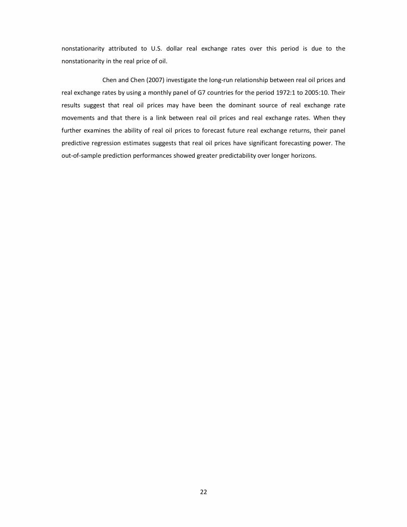
Chen and Chen (2007) investigate the long-run relationship between real oil prices and
real exchange rates by using a monthly panel of G7 countries for the period 1972:1 to 2005:10. Their
results suggest that real oil prices may have been the dominant source of real exchange rate
movements and that there is a link between real oil prices and real exchange rates. When they
further examines the ability of real oil prices to forecast future real exchange returns, their panel
predictive regression estimates suggests that real oil prices have significant forecasting power. The
out-of-sample prediction performances showed greater predictability over longer horizons.

23
Chapter 5: Methodology
5.1 Source of data and information
In this study, quarterly data of industrial production index (henceforth “industrial production”), real
effective exchange rate index15
(henceforth “real exchange rate”), real long term interest rate
(henceforth “real interest rate”), and inflation rate were obtained from Organization for Economic
Cooperation and Development (OECD) database (Data from Main Economic Indicator). The oil price
variable used in this study is World oil price which were obtained from International Financial
Statistics (International Monetary Fund). Data used in “Peak theory” charts was obtained from BP
Statistical Review 2011. The source of other data used for descriptive purposes (charts, tables etc) is
shown below each chart and table in the text. The majority of articles regarding earlier studies on
this subject were obtained from EconLit (Karlstad University, Library section on the internet), other
articles were obtained by Google search.
5.2 The way the variables are used
The variables in this study were originally defined as followed: Oil price variable as nominal US dollars
per barrel, Industrial production and real exchange rates as indexes while inflation rate and real
interest rates as annual rates. As a first step, the oil price variable and real interest rate were
converted into real terms (using US CPI for the oil price variable and the inflation rate for the
respective country to convert the interest rates). As a second step, the variables oil price, industrial
production and real exchange rates were transformed to natural logarithm.
The variables were then used in different ways depending on which analysis is
conducted, for instance, to calculate correlations between oil price and real exchange rates the
following return formula was used for:
∆� ���������� ������� � ln��!� " ln��!#$� [1]
The correlation coefficient between oil price changes and changes in industrial production were
calculated using the following return formula:
∆� ������� ������� � ln��!� " ln ��!#%� [2]
The above specification gives us the annual change of the variables, i.e. change since same quarter of
previous year. In addition, I used the forth lag of the oil variable when calculating the correlation
coefficient between oil price change and the growth in industrial production. The reason for this
15
Real effective exchange rate is the relative price level of one country, evaluated using baskets of goods and services of
several major trading partners (Multilateral rate).

24
transformation is that according to the literature on this subject, the greatest effect of oil prices and
economic activity is observed after one year; see for example Hamilton (2000), Cundao and Perez de
Garcia (2003), Lescaroux and Mignon (2008), among others. It is however not true that the other
variables considered in this study (real exchange rate, real interest rate and inflation rate) should
share the same characteristics as industrial production, i.e. that the effect of oil prices would be
observed after a year. The effect on these variables, if any, is likely to be observed straight away.
In this study, I also use a different specification of oil shock variable, the Net Oil Price
Increase or NOPI specification, in order to determine the magnitude of the contribution to industrial
production index. This specification has been widely used in the literature on this subject, see for
example Hamilton (2003) or Cundao and Perez de Garcia (2003) among others. Hamilton (1996)
argues that if one would like to measure how unsettling an increase in the price of crude oil is likely
to be for the spending decision of consumers and firms, it is more appropriate to compare the
current price with the price over the previous years rather than during the previous year alone. He
thus proposes the following specification:
&'()! � max -0, ln��0�!� " ln�max��0�!#%, �0�!#1, �0�!#$2, �0�!#$3��4 [3]
5.3 Empirical Models
5.3.1 Correlations
As a first step of the empirical analysis, the correlation coefficients are calculated between the oil
price variable and the other variables. These correlations are calculated for the full sample period; in
the case of industrial production, 1966q1-2011q1, in the case of real exchange rate, 1970q1-2011q1,
in the case of real interest rate, 1965q1-2011q1, and in the case of inflation rate, 1966q1-2011q1.
The samples are then divided into two subsamples in order to investigate the correlations before and
after 1986, i.e. before and after the oil price collapse in the mid 1980s. This part of the analysis is
conducted for all countries for which data was available and for which there was enough data in the
pre and post 1986 to calculate the correlations.
5.3.2 Oil shock´s contribution to industrial production
As a measure of oil price shock´s contribution to the growth of industrial production, I will adapt the
nonlinear specification16
used in Hamilton 2003 (equation 3.8) for each of the countries considered:
)()! � 5 6 )()!#$ 6 )()!#2 6 )()!#7 6 )()!#%
6 &'()!#$ 6 &'()!#2 6 &'()!#7 6 &'()!#% [4]
16
The key result of that specification (equation 3.8 in Hamilton 2003) was a regression of quarterly GDP growth on a
constant, 4 lags of GDP and 4 lags of the “net oil price increase NOPI”.

25
This is basically a regression of real quarterly IPI growth on a constant, 4 lags IPI growth and 4 lags of
the oil price measure NOPI. To calculate the size of the contribution, I calculate for each quarter in
the episode the difference between the first quarter ahead forecast implied by the equation above,
and what that first quarter ahead forecast would have been if the oil price measure NOPI had instead
been equal to zero, and take this difference as a measure of the contribution of the oil shock to that
quarter´s IPI growth. This part of the analysis is conducted for all countries for which data on
industrial production were available from 1970.
Due to the unavailability of the data for some of the variables and countries
considered in this study, further analysis (unit root tests, cointegration tests, impulse response
analysis and variance decomposition analysis) will only include the countries; Australia, Belgium,
Canada, France Germany, Italy, Netherlands, Switzerland, United Kingdom and United States. The
time span is set to 1970q1-2011q1 except for Australia and United Kingdom for which real exchange
rate were only available from 1972q1.
5.3.3 Unit Root tests
As a next step in the analysis, unit root tests are carried out in order to investigate the stationarity of
the series considered. Here I will apply the traditional Phillips Peron test (PP), which is closely related
to the Augmented Dickey Fuller test (ADF).
The Dickey Fuller test (DF) involves fitting the model:
�! � 8 6 9�!#$ 6 :� 6 �! [5]
by ordinary least squares (OLS), perhaps setting α=0 or δ=0. However, this regression is likely to be
plagued by serial correlation. To take this into account, the augmented Dickey Fuller test (ADF) test
instead fits the following model:
∆�! � 8 6 ;�!#$ 6 :� 6 <$∆�!#$ 6 <2∆�!#2 6 = 6 <>∆�!#> 6 ?! [6]
Where k is the number of lags to include in the regression. Testing β=0 is equivalent to testing ρ=0, or
equivalently, that �! follows a unit root process. The Phillips Perron test involves fitting [6], and the
results are used to calculate the test statistics. This test statistics can be viewed as Dickey Fuller
statistics that have been made robust to serial correlation by using Newey-West heteroskedasticity-
and autocorrelation-consistent covariance matrix estimator, Gujarati (2002).
The advantages of the PP test over the ADF are; the PP test is robust to general forms of
heteroskedasticity in the error term and the user does not have to specify a lag length for the test
regression. There is however problems associated with the PP test too. A well known weakness of

26
the ADF and the PP tests is theirs potential confusion of structural breaks in the series as evidence of
non-stationarity. In other words, they may fail to reject the null of unit root if the series have a
structural break. It would mean, series that are found to be I(1), there may be a possibility that they
are in fact stationary around the structural break(s), I(0), but are erroneously classified as I(1).17
Also,
the power of the test diminishes as deterministic terms are added to the regression. That is, tests
that include a constant and trend in the regression have less power than tests that only include a
constant in the regression. As a complement to the PP test, this study also applies the Zivot and
Andrews (1992) test which takes into account that the series might contain structural breaks as for
example the oil price shocks in the oil price series. Their procedure involves fitting the following
model:
∆�! � 8 6 ;� 6 �9 " 1��!#$ 6 <AB!�C� 6 ∑ EF>FG$ ∆�!#F 6 �! [7]
Where AB�C� � 1 for � H �C, and otherwise AB � 0; C � �J/� represents the location where the
structural break lies: � is the sample size and �J is the date when the break occurred. In both tests,
PP and Andrews Zivot, the null hypothesis is that the variable has a unit root. Rejection of the null
hypothesis would mean that the series is stationary.
5.3.4 Cointegration tests
To investigate the long term links between oil price and the other variables considered in this study, I
proceed with cointegration tests. Various tests have been suggested in the literature for this
purposes, most of which are implemented in standard econometric packages and hence are easily
available nowadays. Some well known examples include the residual-based Engle and Granger
(1987), henceforth EG, or the system-based tests of Johansen (1988), henceforth J. Error-Correction-
based tests have also been suggested by Boswijk (1994), henceforth Bo, and Banerjee et al. (1998),
henceforth Bo, to name just few. Often one test rejects the null whereas another test does not,
making it unclear how to interpret the outcomes of the tests.
In general, the p-values of different tests are typically not perfectly correlated,
Gregory et al. (2004). Bayer and Hanck (2009), suggest that after running the above tests separately,
one should test the underlying tests in combination in order to reach the right decision. Their
combing tests have shown that when the underlying tests have similar power, the combined results
are even more powerful than the best underlying test.18
Instead of presenting the underlying tests
17
Unit Roots, Structural Breaks and Cointegration Analysis: A Review of the Available Processes and Procedures and an
Application. Workshop, Department of Banking and Finance Faculty of Business and Economics, Eastern Mediterranean
University. 18
They applied their tests to 159 data sets from published Cointegration studies and the result showed that in one third of
all cases, single tests give conflicting results whereas the combining tests provided an unambiguous test decision.
27
and the combined tests here, the interested reader is advised to consult the paper of Bayer and
Hanck (2009) where they explain the models in more detail. In all cases above, he null hypothesis is
no cointegration, rejection of the null would mean that the variables are cointegrated, i.e. there is a
long term relationship between the variables.
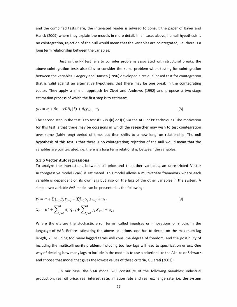
Just as the PP test fails to consider problems associated with structural breaks, the
above cointegration tests also fails to consider the same problem when testing for cointegration
between the variables. Gregory and Hansen (1996) developed a residual based test for cointegration
that is valid against an alternative hypothesis that there may be one break in the cointegrating
vector. They apply a similar approach by Zivot and Andrews (1992) and propose a two-stage
estimation process of which the first step is to estimate:
�$! � 8 6 ;� 6 <AB!�C� 6 E!�2! 6 �! [8]
The second step in the test is to test if �! is I(0) or I(1) via the ADF or PP techniques. The motivation
for this test is that there may be occasions in which the researcher may wish to test cointegration
over some (fairly long) period of time, but then shifts to a new long-run relationship. The null
hypothesis of this test is that there is no cointegration; rejection of the null would mean that the
variables are cointegrated, i.e. there is a long term relationship between the variables.
5.3.5 Vector Autoregressions
To analyze the interactions between oil price and the other variables, an unrestricted Vector
Autoregressive model (VAR) is estimated. This model allows a multivariate framework where each
variable is dependent on its own lags but also on the lags of the other variables in the system. A
simple two variable VAR model can be presented as the following:
L! � 8 6 ∑ ;M>MG$ L!#M 6 ∑ <M>MG$ N!#M 6 �$! [9]
N! � 8O 6 P EM>
MG$L!#M 6 P <M
>
MG$N!#M 6 �2!
Where the u´s are the stochastic error terms, called impulses or innovations or shocks in the
language of VAR. Before estimating the above equations, one has to decide on the maximum lag
length, k. Including too many lagged terms will consume degree of freedom, and the possibility of
including the multicollinearity problem. Including too few lags will lead to specification errors. One
way of deciding how many lags to include in the model is to use a criterion like the Akaike or Schwarz
and choose that model that gives the lowest values of these criteria, Gujarati (2002).
In our case, the VAR model will constitute of the following variables; industrial
production, real oil price, real interest rate, inflation rate and real exchange rate, i.e. the system

28
constitutes of five equations. For instance, the equation for industrial production equation has the
following form:
)Q! � 8$R 6 8$$)Q!#$ 6 = 6 8$>)Q!#> 6 ;$$�!#$ 6 = 6 ;$>�!#> 6 [10] <$$'0�!#$ 6 = 6 <$> '0�!#> 6 :$$ST!#$ 6 = 6 :$> ST!#> 6 E$$)�U�!#$ 6 = 6 E$>)�U�!#>
The choice of the ordering of the variables in the VAR model is also crucial for further analysis as
impulse response and variance decomposition analysis (see below). In practice it is difficult to know
which of the ordering is correct and one has often to consult earlier work on the subject. In this
study, I will adapt a similar ordering19
as suggested by Jimenez-Rodriguez and Sanchez (2004). The
order of the variables is as follow: VAR (Industrial production, real oil price, inflation rate, real
interest rate, and real exchange rate).
VAR has both advantages and drawbacks, Gujarati (2002).
The advantages:
• One does not have to worry about determining which variables are endogenous and which
ones are exogenous; all variables in VAR are treated as endogenous.
• Estimation is simple; usual OLS can be applied to each equation in the system separately.
• Forecasts obtained from VAR are often better than those obtained from the more complex
simultaneous-equation models.
The drawbacks:
• Unlike simultaneous-equation models, a VAR model is a-theoretic because it uses less prior
information. In simultaneous-equation models, exclusion or inclusion of certain variables
plays a crucial role in the identification of the model.
• VAR models are less suited for policy analysis.
• Difficulties in choosing the appropriate lag length.
• All the variables should be stationary, if not, we will have to transform the data (e.g., by first-
differencing).
• Individual coefficients in the estimated VAR models are often difficult to interpret,
practitioners of this technique often estimate the so called impulse response function (IRF).
19
They used the following order: VAR (real GDP, real oil price, inflation, short-term interest rate, long-term interest rate,
real wage, and real effective exchange rate).

29
5.3.5.1 Granger Causality
Next, to investigate the short-term links between oil price and the other variables, I proceed with
bivariate Granger causality test. Granger causality tests are usually performed in the context of
vector autoregressions (VAR) or more specifically, individual equations within VAR systems.
Individual equations in VARs are known as autoregressive distributed lag (ADL) relationships and may
be represented as:
�! � � 6 ∑ �FVFG$ �!#F 6 ∑ WF
VFG$ T!#F 6 A! 6 �!, �� � 1, … , �� [11]
Where �! and T! respectively refer to the variables to be analyzed. A! refer to other variables that
need to be controlled for, if any. The null hypothesis is that T! does not Granger-cause �! amounts to
testing whether WF � 0 for 0 � 1, … , Q. The rationale for conducting such a test is simple. If event X is
seen as causing event Y, then event X should precede Y, Hamilton (1994).
5.3.5.2 Impulse response analysis
One interesting feature of VAR methodology is studying the so called impulse response function
(IRF). The IRF traces out the response of the dependent variable in the VAR system to shocks in the
error terms, such as the u´s in the [9] equations. Suppose u1 in the Y equation increases by a value of
one standard deviation. Such a shock or change will change Y in the current as well as future periods.
But since Y appears in the X equation, the change in u1 will also have an impact on X. Similarly, a
change of one standard deviation in u2 of the X equation will have an impact on Y, Gujarati (2002).
The IRF traces out the impact of such shocks for several periods in the future, in our case 16 quarters
or 4 years.
5.3.5.3 Variance decomposition analysis
Another interesting feature of VAR methodology is to analyze the forecast-error variance
decomposition (FEVD) which measures the fraction of the forecast-error variance of an endogenous
variable that can be attributed to orthogonalized shocks to itself or to another endogenous variable
in the model for b=1,2,… (b-step-ahead variance decomposition). In our case we want to analyze the
contribution of variability due to an oil price shock to the other variables considered in this study
(industrial production, long-term interest rate, real effective exchange rate and inflation rate). The b-
step-ahead is set to 4 quarters or one year.
5.3.6 Hubbert peak theory
The Hubbert peak theory is based on the observation that the amount of oil under the ground in any
region is finite, therefore the rate of discovery which initially increases quickly must at some time
reach its maximum and then starts to decline. The theory is named after the American geophysicist

30
0,0
0,5
1,0
1,5
2,0
2,5
3,0
3,5
4,0
1900
1905
1910
1915
1920
1925
1930
1935
1940
1945
1950
1955
1960
1965
1970
1975
1980
1985
1990
1995
2000
2005
2010
Billion barrels/year
Hubbert predicts that production in the U.S. will peak in late 1960s or early
1970s.
Production peaks in the U.S. in 1970, at 3.52
billion barrels per year.
M. King Hubbert, who created a method of modeling the production curve given an assumed
recovery volume. On the basis of his theory, in a paper20 he presented to the American Petroleum
institute in 1956, he correctly predicted that production of oil from conventional sources would peak
in the U.S. around 1965-1970.
His predictions were dismissed at first; however in 1970 the U.S. produced 3.52 billion
barrels and from that point and forward production started to decline just as Hubbert postulated.
The accuracy of his prediction astonished oil executives. As production continued to decline in the
1980s and 1990s, the concept of peak production turned into a reality. Hubert used complex
differential equations to model the production of oil based on the quantity of oil already produced in
the country. A method which simplifies the calculation of the curve known as Hubbert Linearization
will be used in this paper. This method uses simple mathematics to uncover the key features of the
Hubbert Curve, which was developed first by Professor Kenneth Deffeyes21. Basically, the area under
the curve represents all of the oil that will be produced from the country or the field in question. The
peak of the curve represents the time period at which half of the available oil has been produced.
The Hubert peak theory makes it possible to estimate what percentage of oil has been produced and
also predicts annual production volumes. The method is described in more detail in A12.
20
http://www.hubbertpeak.com/hubbert/1956/1956.pdf 21
Kenneth S. Deffeyes is Professor Emeritus at Princeton University. Before joining the Princeton faculty in 1967, he
conducted research at the Shell Oil research laboratory in Houston and taught at the University of Minnesota and Oregon
State University. He is perhaps best known for his research in the area of Physical Geology. For more information visit:
http://www.princeton.edu/hubbert/
Figure 16. U.S. peak production and Hubbert´s prediction.

31
Chapter 6: Empirical analysis
6.1 The macroeconomic relationship
6.1.1 Correlations
I start the analysis by examining the correlation coefficient between oil price and the other variables
considered in this study. These are presented in Table 1 (A2). Before analyzing the results, the
correlation coefficient is considered to be significant if it exceeds -/+ 0.30. The results for industrial
production shows the expected negative sign for all countries and sub samples except for
Switzerland in the second subsample (1986-11) and for Norway during the first subsample (1966-85)
and during the full sample period (1966-11) which suggest that Norway´s industrial production was
less responsive to oil price shocks during the first subsample compared to the other countries in the
sample. Considering the countries with negative correlation coefficients, in the first subsample
(1966-85), correlations were in the range -0.124 (Greece) to -0.664 (Luxembourg), while in the
second subsample (1986-11) the coefficient is in the range -0.004 (Austria) to -0.401 (Australia). In
general, the negative correlation coefficients for most of the countries in the sample are lower in
magnitude for the period post 1986 which suggest that these countries industrial production is less
responsive to oil price shocks post the mid 1980s.
The results for inflation rate show the expected positive sign for all countries in the
first subsample (1966-85) except for Mexico. The positive correlation coefficient ranges from 0.008
(Norway) to 0.659 (Japan) in the first subsample (1966-85), while in the second subsample (1986-11)
the coefficient is in the range -0.215 (Turkey) to 0.463 (United States). The correlation coefficient
turned from being positive in the first sub sample to negative in the second sub sample for about half
of the countries in the sample. The overall results indicate that the pass through effect from
increasing oil prices to consumer prices is much lower today than in the 1970s. There are however
some countries in the second subsample that still have high positive correlations (compared to the
other countries in the sample) such as Belgium and the United States. This is explained by the higher
weights’ given to fuels and heating oil in constructing the CPI index for these countries.
The results for real exchange rates are mixed, reflecting if the country in question
being net importer/exporter. Since oil price is nominated in USD, a weakening of the USD leads to
increase in oil price. In fact it is widely believed that one of the contributing factors to the latest
increase in oil prices (2002-2008) was due to the weakening of the US economy and the dollar value.
This is demonstrated by the correlation coefficient for the US case in the second subsample (-0.345).
On the other hand, the correlation coefficient for Canada and Norway is positive as one would
expect, these two countries are key suppliers of oil among the OECD countries, so when oil price

32
increases their currencies appreciates. Also, these two countries coefficients are lower during the
first subsample (1970-86) which basically reflects these two countries share of world oil supply
during this period. Australia´s coefficient is also high during the second subsample (1986-11),
however not because the country is net exporter of oil but because the country is the third largest
producer of gold in the world and gold prices have historically followed oil prices quite well.
Considering the result of the correlation between oil price and real interest rates, the
majority of the countries show a negative correlation, although too low to be considered as
significant. In the second sample, the United States stands out for having the most negative
coefficient among the countries, -0.367. This clearly illustrates the mechanisms between these two
variables discussed in chapter 3.3, i.e. high/low interest rates put downward/upward pressure on oil
price through different channels. Also to note, that the coefficient for the US is smaller in the first
subsample (1965-85) than the second sample (1986-11) which suggest that the impact have
strengthen post 1986.
6.1.2 Oil shock´s contribution to industrial production
To illustrate the contribution of earlier oil price shocks to industrial production, I used the model
described in chapter 5.3.2., which results are presented in Table 2 in A3. Although the model´s
simplicity, the model did quite well in illustrating the magnitude of these shocks. As one would
expect and following the discussion in chapter two, the contribution was larger during the first two
shocks than during the shock in 1990 and 2008. During the first shock the negative contribution was
ranging from -0.3 percent (United Kingdom) to -3.3 percent (Luxembourg), during the second shock -
0.7 percent (Germany) to -3.0 percent (Luxembourg), during the third shock -0.1 (Finland and France)
to -0.6(Greece), and during the latest shock -0.3 percent (Sweden) to -1.1 (Greece and Japan).
The model also predicted that the contribution to Norwegian industrial production is
positive during all previous shocks. The result for Norway is also in line with the correlation
coefficient provided in Table 1 in A2, i.e. during the first subsample (1966-85) the correlation
coefficient was +0.154 while in the second subsample (1986-11) it turned to -0.155, compared to the
contribution of +0.6 percent during the first shock and +0.2 percent during the latest shock. The
results thus suggest that the positive impact on Norwegian industrial production was larger during
the first two shocks compared to the one in 1990 and 2008.
6.1.3 Unit Root tests
To test the series for unit root, two different tests were used in this study. The first test is the
traditional Phillips Peron test (PP) which is robust to general forms of heteroskedasticity in the error
term. The second test is the Zivot and Andrews test (ZA) which takes into account that the series

33
might contain structural breaks; this is likely to be the case since we are analyzing series with very
long time span. The results of these tests are presented in Table 3-6 in A4. In both tests, the null
hypothesis is that the variable has a unit root and a rejection of the null hypothesis would mean that
the series are stationary. Considering the results provided by the PP test, the null hypothesis is not
rejected for most variables and countries indicating that these variables are non-stationary in level
form. Exceptions are represented by the industrial production for Belgium, Germany, Netherlands,
by the inflation rate for Italy and by the real exchange rate for France and Switzerland which all
appear to be stationary in levels (when considering the model with constant and trend). The null
hypothesis is rejected for all variables and countries when expressed in first differences.
Allowing for breaks in both constant and trend, the results for the ZA test shows that
the oil price variable is non-stationary in level form. Industrial production and real exchange rate are
also non-stationary for all countries with the exception for the industrial production for France,
Germany and the Netherlands and for the real exchange rate for Italy. The results for real interest
rate and inflation rate suggest that for most countries, the variables are stationary in levels. In fact,
the result for real interest rate and inflation rate did not change much using the model which only
allows for break in the constant term, thus the result suggest that in general, real interest rate and
inflation rate are stationary in levels but around the specified break. The null hypothesis is rejected
for all variables and countries when expressed in first differences.
6.1.4 Cointegration tests
To investigate the long-term link between oil price and the other variables, I proceed with
cointegration tests. Two variables are said to be cointegrated if they have a long-term, or equilibrium
relationship between them. In this paper I test for cointegration using two tests; the first test is the
Bayer and Hanck test which is a combined test of individual cointegration tests. The second test is
the Gregory Hansen test which takes into account the possibility of structural breaks in the data. The
null hypothesis of both tests are no cointegration, therefore, a rejection of the null hypothesis means
that the two series are cointegrated. The results of these tests are presented in Table 7-8 in A5.
Considering the results provided by the Bayer Hanck Test (the combined test for the individual tests);
oil price and industrial production are cointegrated for Australia, Belgium, Germany, Italy and
Switzerland. Cointegration is also found between oil price and real interest rate for Germany,
Switzerland and United States. The result leads to the same conclusion when using both EG-J and EG-
J-Ba-Bo.
In the case of oil price and inflation rate, the first test statistic (EG-J) does not reject
the null hypothesis of no cointegration for all countries accept for Canada and Switzerland. The null is
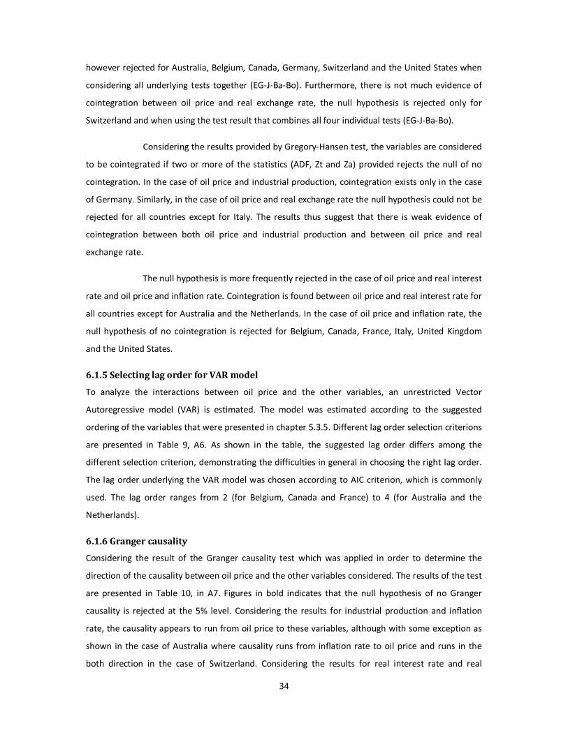
34
however rejected for Australia, Belgium, Canada, Germany, Switzerland and the United States when
considering all underlying tests together (EG-J-Ba-Bo). Furthermore, there is not much evidence of
cointegration between oil price and real exchange rate, the null hypothesis is rejected only for
Switzerland and when using the test result that combines all four individual tests (EG-J-Ba-Bo).
Considering the results provided by Gregory-Hansen test, the variables are considered
to be cointegrated if two or more of the statistics (ADF, Zt and Za) provided rejects the null of no
cointegration. In the case of oil price and industrial production, cointegration exists only in the case
of Germany. Similarly, in the case of oil price and real exchange rate the null hypothesis could not be
rejected for all countries except for Italy. The results thus suggest that there is weak evidence of
cointegration between both oil price and industrial production and between oil price and real
exchange rate.
The null hypothesis is more frequently rejected in the case of oil price and real interest
rate and oil price and inflation rate. Cointegration is found between oil price and real interest rate for
all countries except for Australia and the Netherlands. In the case of oil price and inflation rate, the
null hypothesis of no cointegration is rejected for Belgium, Canada, France, Italy, United Kingdom
and the United States.
6.1.5 Selecting lag order for VAR model
To analyze the interactions between oil price and the other variables, an unrestricted Vector
Autoregressive model (VAR) is estimated. The model was estimated according to the suggested
ordering of the variables that were presented in chapter 5.3.5. Different lag order selection criterions
are presented in Table 9, A6. As shown in the table, the suggested lag order differs among the
different selection criterion, demonstrating the difficulties in general in choosing the right lag order.
The lag order underlying the VAR model was chosen according to AIC criterion, which is commonly
used. The lag order ranges from 2 (for Belgium, Canada and France) to 4 (for Australia and the
Netherlands).
6.1.6 Granger causality
Considering the result of the Granger causality test which was applied in order to determine the
direction of the causality between oil price and the other variables considered. The results of the test
are presented in Table 10, in A7. Figures in bold indicates that the null hypothesis of no Granger
causality is rejected at the 5% level. Considering the results for industrial production and inflation
rate, the causality appears to run from oil price to these variables, although with some exception as
shown in the case of Australia where causality runs from inflation rate to oil price and runs in the
both direction in the case of Switzerland. Considering the results for real interest rate and real

35
-0,006
-0,004
-0,002
0,000
0,002
0,004
0 4 8 12 16
Industrial production
-0,008
-0,004
0,000
0,004
0,008
0,012
0 4 8 12 16
Real exchange rate
exchange rate, there is not enough evidence to conclude the direction of the causality. In the case of
real interest rate, causality runs from oil price to real interest rate for Belgium, Italy and Switzerland,
whereas it runs from real interest rate to oil price for Australia, Germany. In the case of real
exchange rate, causality runs from oil price to real exchange rate for Netherlands, United Kingdom
and the United States, and it runs from real exchange rate to oil price in the case for Australia.
Furthermore, causality runs in the both direction for Germany.
6.1.7 Impulse response analysis
I continue the analysis by analyzing the results from the impulse response to assess the impact of a
shock in real oil price on industrial production, real interest rates, real exchange rates and inflation
rates. The results for the US are presented below in Figure 17-18; the results for the other countries
are presented in A8 in Figures 21-25. In particular, the impulse response function traces over time
the effects on a variable of an exogenous shock to another variable (the solid line). The dash line is
the 95% confidence error bands for the IRFs which are provided to judge the statistical significance of
the impulse response functions.
Considering industrial production, the impulse response functions indicates that an oil
price shock is followed by declining industrial production where the biggest fall occurring in the third
or fourth quarter after the shock excepts for Belgium where the biggest fall occurring in the fifth
quarter. The contemporaneous affect22
is zero for all countries as one would expect (industries do
not react immediately to an oil price shock), also the effect tends to die out after 5-8 quarters from
the shock. Moving forward and considering the results for real interest rate, the impulse response
functions shows that the contemporaneous affect is negative and significant for Belgium, France,
Italy, Switzerland and United States. The functions also shows that these rates start to increase
following the shock, as seen in the case for Canada, France and the United States. The rates also
increase for the other countries, however not immediately, but after 2-3 quarters.
22
The immediate effect.
Figure 17. The figure presents the orthogonalised impulse-response function of Industrial production and Real
exchange rate for United States.

36
-0,002
0,000
0,002
0,004
0,006
0 4 8 12 16
Inflation rate
-0,004
-0,002
0,000
0,002
0 4 8 12 16
Real interest rate
The effects on real exchange rates are different depending on whether the country in question is net
oil importer/exporter. First we observe that the contemporaneous effect for France, Germany, Italy,
Netherlands, Switzerland and the United States is negative however not significant. On the other
hand the contemporaneous effect on the real exchange rate of Canada and Australia is positive and
significant, and for the United Kingdom positive but not significant. These observations clearly
demonstrate the terms of trades’ shocks on these countries real exchange rates following an oil price
shock, i.e. appreciation if terms of trade are improved and depreciation if terms of trade are worsen.
Following the shock, the effect is positive and significant in the first quarter for United Kingdom and
negative and significant in the second quarter for Germany. For all countries in the sample, the effect
tends to die out after four to eight quarters following the shock.
The impulse response functions for the inflation rates shows that the contemporaneous affect is
positive and significant for Belgium, Canada, France, Germany, Italy, Switzerland, United Kingdom
and the United States. In the case of France, Germany, United Kingdom and the United States, the
inflation rate declines gradually after the shock whereas for the rest of the countries the inflation
rates tend to persist for 0-3 quarters (in the case of Belgium, Canada, Italy, Netherlands and
Switzerland). In fact there is an increase in the inflation rate the following 1-2 quarter after the shock
for Italy, Netherlands and Switzerland.
6.1.8 Variance decomposition analysis
In this section, I continue the analysis by analyzing the results from the forecast error variance
decomposition (FEVDs) of industrial production, real interest rate, real exchange rate and inflation
rate due to the oil price variable. Table 11, in A.9, presents the FEVDs for the countries considered.
Each value in the table is in percentage form and shows how much of the unanticipated change in
industrial production, real interest rate, real exchange rate and inflation rate are due to oil price
shock. Also the table provides the t-values (in parentheses) of the computed FEVDs in order to judge
for FEVDs significance.
Figure 18. The figure presents the orthogonalised impulse-response function of inflation rate and real interest rate
for United States.

37
The contribution of an oil price shock to the variability in industrial production varies from 1.3
percent (Canada) to 14.6 percent (United Kingdom). The FEVDs are significant for France, Germany
and the United Kingdom. In the case of real interest rates the contribution varies from 2.4 percent
(Germany) to 18.2 percent (Belgium) and the contributions are significant for Belgium, Italy,
Netherlands and the United States. The FEVDs for real exchange rate shows that the contribution is
in the range 0.6 percent (Italy) to 8.6 percent (Germany), and the FEVDs are significant for Australia
and Germany. Finally the contribution to the variability in inflation rate ranges from 3.0 percent
(Australia) to 35.4 percent (Belgium) and are significant for Belgium, Canada, France, Germany, Italy,
Netherlands, Switzerland and the United States.
6.2 Oil Consumption and Economic growth
One important point in understanding short-run changes in the price of oil is the fact that income
rather than price is the key determinant of the quantity of oil demanded by a country, Hamilton
(2009). To see this, Figure 19 below plots the cumulative change in US real GDP (x-axis) against
cumulative change in oil supplied to the US market (y-axis) for the period 1949-2007. One can
observe that despite the large fluctuations in the price of oil during this period, oil consumption have
followed GDP growth quiet well. Also evident, is that there is flattening in the slope over time and
the downward adjustment in oil demand following the 1970s crises. The slope of 0.47 for the period
1985-97 could be attributed to the downward adjustment during the beginning of the 1980s;
however, it is more likely that the flattening in the slope is due the fact that income elasticity
declines as a country become more developed as illustrated by the slope of 1.04 (1961-73) compared
to the slope of 1.22 (1949-61), i.e. the slope flattens before the OPEC embargo.
Figure 26-28 in A10, plots oil consumption against GDP for some of the other countries
for the period 1965-2010. In addition to these countries, I have included the plots for China and India
as they are considered as important oil consumer today. In general, oil consumption has followed
GDP growth quiet well as in the US case discussed above. Also, the slope coefficient flattens for most
of the countries post the 1980s, however to different extent reflecting each country´s share of oil
consumed in relation to global oil supplied, the ability of each country to switch to alternative
sources of energy and the development of the country. Another factor to bear in mind is that the
country´s attitude towards oil consumption (whether to increase or decrease) is also dependent on
what trading partners the country has. As an example, the Netherlands have substantially increased
its share in oil consumption over the last 10 years, it might seem odd at first; however the

38
0,00
0,20
0,40
0,60
0,80
1,00
1,20
1,40
0,00 0,20 0,40 0,60 0,80 1,00 1,20 1,40 1,60 1,80 2,00 2,20
United States
1949-61: slope 1.22
1961-73: slope 1.04 1985-97:
slope 0.47
Netherlands main source of crude oil imports are from Russia, Norway and Saudi Arabia23, all of
which are not considered today as insecure importing partners.
The Figures 29-30, presents countries for which no slope could be fitted for the period post 1980s.
These countries were quick in switching from oil towards other substitutes after experiencing the
shocks of the 1970s.
As a complement to these figures, the tables 12-13 in A11 (Countries Energy Mix),
presents the average energy mix share used by these countries as of total primary energy demanded
for different periods. Figures in bold indicates that the country in question has increased its share in
the resource in question since previous period. In general, while countries have been efficiently
decreasing their share in oil consumption, they have increased their consumption of another fossil
fuel, namely Natural Gas. Gas is becoming increasingly important for most countries in their energy
mix. As end of 2010, proven gas reserves in North, Central and South America amounted to 9.3
percent, in Europe and Eurasia 33.7 percent (of which 23.9 percent in Russia), in the Middle East 40.5
percent (of which 15.8 percent in Iran and 13.5 percent in Qatar), in Africa 7.9 percent, and in Asia
Pacific 8.7 percent24
. Clearly, Russia, Iran and Qatar are and going to be key suppliers of Gas in the
short and long term. As the share of natural gas in global energy supply increases, it has begun to
create risks factors of its own. Like oil, gas markets are subject to many disruptive geopolitical forces,
including attempts to exercise monopoly power by Russia. After the discontinuance of Russian gas
supplies to the Ukraine in the winter of 2005-06 and again in 2008-09, gas importing countries have
begun to question that natural gas imports will prove more secure than oil. This have prompted
23
http://ec.europa.eu/energy/energy_policy/doc/factsheets/mix/mix_nl_en.pdf 24
BP Statistical Review 2011.
Figure 19. Cumulative change in US GDP (x-axis) against cumulative change in oil
consumption in the US. Source: Hamilton (2009).

39
many consuming countries in Europe to seek diversification as means of mitigating away the
potential risks of being heavily reliant on any single supplier.
By 2040, the internationally traded share of world natural gas demand is projected to
rise to 48 percent, with Liquefied Natural Gas (LNG) shipments responsible for the majority of this
growth. Most of that growth, in turn, is expected to come from the Middle East, Hartley and Medlock
(2006). In other words, as European countries seek to diversify away from Russian natural gas, they
expose their markets to Middle East geopolitical risks which further contribute to the similarities with
oil markets.
Among the OECD countries that have the largest share of renewable source of energy
are Denmark, Sweden, Finland, Portugal and Sweden, all having 4 percent and above. However this
share is too small today to benefit these countries today, as seen from the table, these countries
have no choice but to increase their share of natural gas in the short/medium term until their
renewable sources are developed.
6.3 Depletion analysis
The Hubbert Curves in this paper are drawn using a very simple approach, namely Hubert
linearization. There are other approaches one could use in order to get more accurate curves, see for
example Laherrere (2000), who also points out some strengths and weaknesses with the Hubbert
curve and. A simple Hubbert curve may be ideally applied only in the following cases:
• There should be large populations of fields: the production curve of a single oil field is
generally asymmetrical. However when there is a large population of fields, such that the
sum of a large number of asymmetrical distributions becomes symmetrical (normal) under
the Central Limit Theorem of statistics.
• Exploration should follow a natural pattern unimpeded by political events or significant
economic factors, as an example when OPEC cut production during the embargo in 1973.
• Where a single geological domain having a natural distribution of fields is considered,
political boundaries should be avoided.
Bearing these constraints in mind we can continue to study the results of the curves presented in this
paper. Starting with the US case (Figure 20, below), according to the model, oil production peak was
reached in 1975 whereas actual production peaked in 1970. Ever since production has continued to
decline, and in 2010 the US had produced 87 percent of its total expected output of 232 billion
barrels. The Hubbert peaks for the other countries are presented in A12. Other countries that show a
close pattern between actual production curves and predicted once are Norway and United

40
Kingdom. According to the model Norway´s oil production peak was reached in 2000 which is
consistent with the year, 2000, when actual production peaked. In 2010, Norway had produced 83
percent of its total expected output of 30 billion barrels. For the United Kingdom, oil production peak
was reached in 1994 according to the model; however actual peak occurred in 1999. In 2010, the
United Kingdom had produced 87 percent of its total expected output of 31 billion barrels. The
reason why the model failed in choosing the right year for which UK production peaked is because of
the production disruption occurring prior to the peak as seen in the figure.
Another country which have been following this trend is Indonesia who for long time
been a member of OPEC choose to voluntarily end its membership in 2008 when it became a net
importer of oil. Actual production peak in Indonesia was reached in 1977, model peak was reached in
1990, and in 2010 the country had produced 83 percent of its total expected output of 26 billion
barrels. Again the model failed in choosing the right year of the peak to constraints discussed above.
As for the plots for the other countries, no clear conclusion could be drawn on whether these
countries have reached their peak production or not. It is however important to give this area an
attention since oil is likely not going to be available forever and the challenges will lie in the process
of restructuring towards other substitutes.

41
0,0
0,5
1,0
1,5
2,0
2,5
3,0
3,5
4,0
1900 1920 1940 1960 1980 2000 2020 2040 2060
Billion barrels/year
Actual production
Model prediction
In 2010, the U.S. had produced 87 percent of its total expected output (232 billion barrels). Actual peak was reached in 1970. Model peak
around 1975.
Figure 20. The Hubbert Curve for United States, author calculation. Based on data from BP Statistical Review 2011.
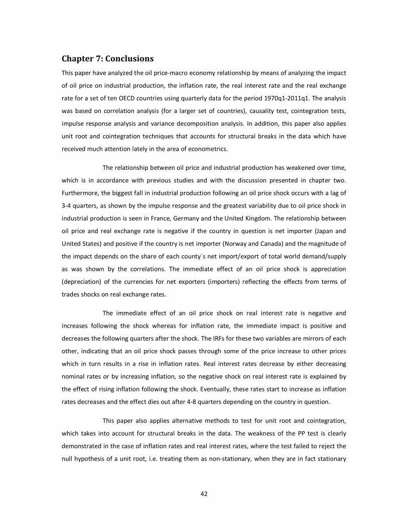
42
Chapter 7: Conclusions
This paper have analyzed the oil price-macro economy relationship by means of analyzing the impact
of oil price on industrial production, the inflation rate, the real interest rate and the real exchange
rate for a set of ten OECD countries using quarterly data for the period 1970q1-2011q1. The analysis
was based on correlation analysis (for a larger set of countries), causality test, cointegration tests,
impulse response analysis and variance decomposition analysis. In addition, this paper also applies
unit root and cointegration techniques that accounts for structural breaks in the data which have
received much attention lately in the area of econometrics.
The relationship between oil price and industrial production has weakened over time,
which is in accordance with previous studies and with the discussion presented in chapter two.
Furthermore, the biggest fall in industrial production following an oil price shock occurs with a lag of
3-4 quarters, as shown by the impulse response and the greatest variability due to oil price shock in
industrial production is seen in France, Germany and the United Kingdom. The relationship between
oil price and real exchange rate is negative if the country in question is net importer (Japan and
United States) and positive if the country is net importer (Norway and Canada) and the magnitude of
the impact depends on the share of each county´s net import/export of total world demand/supply
as was shown by the correlations. The immediate effect of an oil price shock is appreciation
(depreciation) of the currencies for net exporters (importers) reflecting the effects from terms of
trades shocks on real exchange rates.
The immediate effect of an oil price shock on real interest rate is negative and
increases following the shock whereas for inflation rate, the immediate impact is positive and
decreases the following quarters after the shock. The IRFs for these two variables are mirrors of each
other, indicating that an oil price shock passes through some of the price increase to other prices
which in turn results in a rise in inflation rates. Real interest rates decrease by either decreasing
nominal rates or by increasing inflation, so the negative shock on real interest rate is explained by
the effect of rising inflation following the shock. Eventually, these rates start to increase as inflation
rates decreases and the effect dies out after 4-8 quarters depending on the country in question.
This paper also applies alternative methods to test for unit root and cointegration,
which takes into account for structural breaks in the data. The weakness of the PP test is clearly
demonstrated in the case of inflation rates and real interest rates, where the test failed to reject the
null hypothesis of a unit root, i.e. treating them as non-stationary, when they are in fact stationary

43
around a structural break. The test results did not differ much for industrial production and real
exchange rate.
Considering the results from the cointegration tests, individual tests and the combined
test offered by Bayer Hanck show some signs of cointegration between oil price and industrial
production. However, taking into account for structural breaks, the null hypothesis of no
cointegration was not rejected for all countries except for Germany. The null hypothesis of no
cointegration is frequently rejected for oil price and inflation rates and for oil price and real interest
rates when taking account for structural breaks, in fact the results by Bayer Hanck also support the
alternative hypothesis when oil price and inflation rate are considered. Furthermore, the alternative
hypothesis of cointegration between oil price and real exchange rate could not be accepted for most
of the countries and tests.
This paper have also discussed the importance of the terms oil scarcity, peak theory in
order to give an answer to what alternatives source of energy are likely to be substitutable for oil in
the short/long term. The result of the Hubbert curves25 indicates that Australia, Indonesia, Mexico,
Norway, United Kingdom, United States have already reached their oil production peaks and
production in these countries have been declining on yearly basis ever since. In the short term,
renewable source of energy are not likely to dominate OECD countries energy mix26
, instead, there is
a general trend of increasing natural gas consumption among most OECD countries. As the share of
natural gas in global energy increases, it has begun to create risk factors of its own. Like oil, gas
markets are subject to many disruptive geopolitical forces, including attempts to exercise monopoly
power by Russia. Consumer countries have begun to question that gas imports will prove to be more
secure than oil imports. However, as European countries seek to diversify away from Russian natural
gas, they will expose their markets to Middle East geopolitical risks as the majority of future gas is
expected to be supplied by countries in the Middle East.
The term oil scarcity seems to be underestimated, and need more attention than it
received so far and as discussed in chapter 2, Oil scarcity seems not to be reflected in the price of oil.
In general it is expected that if oil prices were to rise, a substitute for the resource would be searched
for and eventually found, but, if the price of oil do not reflect the scarcity of oil, then there is a risk
that this search will be initiated too late. Scarcity may then pose a serious limitation to the economy
before a substitute resource or technology has been found.
25
The Hubbert curves presented in this paper are based on simple method known as Hubbert Linearization, more advanced
method could be used in order to get more accurate results. 26
The data shows however that Scandinavian countries are ahead of many other OECD countries in terms of renewable
source of energy.

44
Suggestions for further studies; There are not many studies conducted on the gas market and its
similarities to the oil markets. This paper has barely touched this area but points out the increasing
interest among OECD countries for gas consumption. The oil price variable used in this paper was
nominated in US dollars, one could extend the analysis and instead use oil price variables nominated
in different exchange rates for the countries considered or use different specifications27
of the oil
price variable (as the NOPI specification described in this paper). Another interesting relationship to
study is the relationship between gold price and oil price (as was seen in the case of Australia).
Finally, this paper highlights the importance of oil scarcity; this area is likely to observe more
attention in the near future as oil becomes scarcer. There are a variety of methods out there for
calculating the Hubbert curves (the simplest one was used in this paper).
27
Other specifications that could be used are for example oil price variable that only includes positive/negative changes.

45
References
Ahrari, Mohammed E. 1986. “OPEC: The Failing Giant”. Lexington: University Press of Kentucky.
Banerjee, A., Dolado, J. J., and Mestre R. (1998). "Error-correction mechanism tests for cointegration in a
single equation framework" Journal of Time Series Analysis, 19(3), 267-283.
Bernanke, B., Gertler, M., and Watson, M., (1997). “Systematic Monetary Policy and the Effects of Oil Price
Shocks”. Brookings Papers on Economic Activity 1997(1), pages 91-157.
Berument, M.H., N.B. Ceylan and N. Dogan (2010). "The Impact of Oil Price Shocks on the Economic Growth of
Selected MENA Countries." The Energy Journal 31: 149-176.
Blanchard, O.J., and Gali, J., (2008). “The Macroeconomic Effects of Oil Price Shocks: Why are the 2000s so
different from the 1970s?” CEPR Discussion Paper DP6631.
Boswijk, H. P. (1994). "Testing for an unstable root in conditional and unconditional error correction models"
Journal of Econometrics, 63, 37-60.
Bronson (2006). "Thicker Than Oil: America´s Uneasy Partnership with Saudi Arabia".
Burbidge, J. and A. Harrison (1984). "Testing for The Effect of Oil Price Rises Using Vector Autoregressions."
International Economic Review 25: 459-484.
Chaudhuri, Kausik, Daniel, Betty C., (1998). "Long-run equilibrium real exchange rates and oil prices".
Economics Letters 58 (2), 231-238.
Chen, S-S., and Chen, H-C. (2007). "Oil prices and real exchange rates". Energy Economics 29 (2007) 390-404.
Clark, T.E., and Terry, S.J., (2009). “Time Variation in the Inflation Passthrough of Energy Prices”. Federal
Reserve Bank of Kansas City, Research Working Paper RWP 09-06.
Coudert, V., Coubarde, C and Mignon, V (2009). “Terms Of Trade And Exchange Rates: A Relationship
Complicated By Anchor Policies”. CEPII, No 285.
Cunado, J. and F. Perez de Garcia (2003). "Do Oil Price Shocks Matter? Evidence for some European countries."
Energy Economics 25: 137-154.
Darby, M. R. (1982). "The Price of Oil and World Inflation and Recession." American Economic Review 72: 738-
751.
Edahiro, Junko (2010). "CO2 Emissions from the Japanese Transport Sector Already Decreasing": JFS Newsletter
No.95 (July 2010).
El-Gamal, M and A.M. Jaffe (2010). "Oil, Dollars, Debt, and Crises: The Global Curse of Black Gold". Cambridge
University Press.
Engle, R. F., and Granger, C. W. J. (1987). "Cointegration and error correction: Representation, estimation, and
testing" Econometrica, 55(2), 251-76.
Fraum, D. (2002). "How We Got Here: The 70s" Basics Books.
Fusco, Leha (2006). "Energy Policy Development in the Globalized World: A Comparison of the USA, Canada,
Britain and Norway". Occasional paper no.1 of the Project, "Oil, Power and Dependency: Global and Local
Realities of the Offshore Oil Industry in Newfoundland and labrador"
Gaudet, G. (2007). “Natural Resource Economics under the Rule of Hotteling”. Département de sciences
économiques and CIREQ. Université de Montréal.

46
Gisser, M. and T. H. Goodwin (1986). "Crude Oil and the Macroeconomy: Tests of Some Popular Nations."
Journal of Money, Credit and Banking 18: 95-103.
Gregory, A. W., Haug, A. A., and Lomuto, N. (2004). "Mixed signals among tests for cointegration" Journal of
Applied Econometrics, 19(1), 89-98.
Gujarati, Damodar N, (2000). "Basic Econometrics", fourth edition. McGraw-Hill Higher Education.
Hamilton, J. D. (1983). "Oil and the Macroeconomy since World War II." Journal of Political Economy 91: 228-
248.
Hamilton, J. D. (1994). "Time Series Analysis". Princeton University Press.
Hamilton, J. D. (2000). "What is an oil shock?" NBER working paper series no. 775
Hammes, D. and D. Wills (2005). "Black Gold: The End of Bretton Woods and the Oil-Price Shocks of the 1970s."
Independent Review 9: 501-511.
Hartley, P. and K. Medlock. (2006). "Political and Economic Influences on the future World Market for Natural
Gas", Cambridge University Press.
Helbling, Hans H. and James E. Turley (1975). "Oil Price Controls: A Counterproductive Effort." Federal Reserve
Bank of St. Louis Review 57: 2-6.
Ikenberry, G. John (1986). "The irony of the state strength: comparative response to the oil shocks in the
1970s." International Organization 40: 105-137.
Jimenez-Rodriguez, R. and M. Sanchez (2005). "Oil Price Shocks and Real GDP Growth: Empirical Evidence for
Some OECD Countries." Applied Economics 37: 201-228.
Johansen, S. (1988). "Statistical analysis of cointegration vectors" Journal of Economic Dynamics and Control,
12(2-3), 231-254.
Kilian, L., and Lewis, L., (2009). “Does the Fed Respond to Oil Price Shocks?”. CEPR Discussion Paper DP7594.
Laherrere, J.H. (2000). "The Hubbert Curve: Its Strengths And Weaknesses" version proposed to Oil and Gas
Journal on Feb 18 2000.
Lai Kon S. (2008). "The puzzling unit root in the real interest rate and its inconsistency with intertemporal
consumption behavior". Journal of International Money and Finance 27 (2008) 140-155.
Lescaroux, F. and V. Mignon (2008). "On the Influence of Oil Prices on Economic Activity and Other
Macroeconomic and Financial Variables." CEPII research, Working Papers 200805: 343-380.
Licklider, R. (1988). "The Arab Oil Weapon and the Netherlands, the United Kingdom, Canada, Japan and the
United States." International Studies quarterly 32: 205-226.
Mork, K. O. Olsen, and H. Mysen (1994). "Macroeconomic Responses to Oil Price Increases and Decreases in
Seven OECD Countries." The Energy Journal 15: 19-35.
O´Sullivan, M. (2003). "Shrewd Sanctions: Statecraft and state Sponsors of Terrorism. Washington, DC: The
Brookings Institution Press.
Pindyck R. S., and Rotemberg J. J. (1983). “Dynamic Factor Demands and the Effects of Energy Price Shocks.
American Economic Review, 73, pp. 1066-79.
Rasche, R. H. and J.A. Tatom (1977). "The Effects of the New Energy Regime on Economic Capacity, Production
and Prices." Federal Reserve Bank of St.Louis Review 59(4): 2-12.
Rasche, R. H. and J.A. Tatom (1981). "Enegy Price Shocks, Aggregate Supply and Monetary Policy: The Theory
and International Evidence." Carnegie-Rochester Confernence Series on Public Policy 14: 125-142.

47
Reicher, C.P., and Utlaut, J. (2010). “The relationship between oil prices and long-term interest rates”. Kiel
Institute Working Papers No. 1637, July 2010.
Santini, D.J. (1985). "The Energy-Squeeze Model: Energy Price Dynamics in U.S. Business Cycles." International
Journal of Energy Systems 5: 18-25.
Snowdon, B., Vane, H., & Wynarczyk, P. (1994). “A modern guide to macroeconomics”. (pp. 236-79).
Cambridge: Edward Elgar Publishing Limited.
Spiro, D. (2011). "Resource extraction, capital accumulation and time horizon", Institute for International
Economic Studies, IIES.
Zhou, Su,. (1995). "The response of real exchange rates to various economic shocks". Southern Economic
Journal 61 (4), 936-954.
Zivot, E., Andrews, D., (1992). "Further evidence on the great crash, the oil-price shock, and the unit-root
hypothesis". J. Bus. Econ. Stat. 10, 251-270.
Internet:
BP- http://www.bp.com
Eurostat- http://epp.eurostat.ec.europa.eu
International Energy Agency- http://www.iea.org/
International Monetary Fund- http://www.imf.org
Karlstads Universitetsbibliotek- http://www.kau.se/bibliotek
Organization for Economic Co-operation and Development- http://www.principalglobalindicators.org
The World Bank- http://www.worldbank.org/

48
Appendices
A1. Data
The data used to analyze the relationship between oil prices and the other macroeconomic variables
(Industrial production, real long-term interest rate (“real interest rate”), real effective exchange rate
(“real exchange rate”) and inflation rate) were obtained from Organisation for Economic Co-
operation and Development (OECD). The countries for which correlations are calculated cover most
OECD countries where data were available (see below). The unit root, cointegration and VAR analysis
covers the countries: Australia, Belgium, Canada, France, Germany, Italy, Netherlands, Switzerland,
United Kingdom and United States.
• Real oil price: World oil price, defined as the quarterly average nominal price was deflated
by the U.S. quarterly CPI. The two series cover the period: 1965q1-2011q1.
• Industrial Production: Total Industrial production index was used as an indicator of economic
activity. Length of the series: Australia, Austria, Belgium, Canada, Finland, France, Germany,
Greece, Italy, Japan, Luxembourg, Netherlands, Norway, Portugal, Sweden, Switzerland,
United Kingdom and the United States cover the period 1965q1-2011q1. For Denmark, data
was only available from 1974q1. For Hungary, Ireland, Mexico, New Zealand, Poland and
Turkey from 1985q1.
• Exchange Rate: Real Effective Exchange Rates was used in order to better reflect each
individual country´s currency value relative to other currencies. The series are quarterly.
Length of the series: Austria, Belgium, Canada, Denmark, Finland, France, Germany, Greece,
Iceland, Ireland, Italy, Japan, Luxembourg, Mexico, Netherlands, New Zealand, Norway,
Portugal, Spain, Sweden, Switzerland, Turkey and the United States cover the period
1970q1-2011q1. For Australia and United Kingdom the series was only available from
1972q1.
• Real Long term interest rate: Long term (nominal) government bonds rate was converted
into real term using the CPI of each country. The series are quarterly. Length of the series:
Australia, Belgium, Canada, France, Germany, Italy, Netherlands, Switzerland, United
Kingdom and United States cover the period 1965q1-2011q1. For Ireland, New Zealand,
Norway and Spain, the series was only available from 1986q1. For Denmark and Sweden
from 1987q1, for Finland from 1988q1 and for Japan from 1989q1.
• Inflation rate: The series are quarterly (annual rates). Length of the series: Australia, Austria,
Belgium, Canada, Denmark, Finland, France, Germany, Greece, Iceland, Ireland, Italy, Japan,
Luxembourg, Mexico, Netherlands, New Zealand, Norway, Portugal, Spain, Sweden,

49
Switzerland, Turkey, United Kingdom and United States cover the period 1965q1-2011q1.
For Hungary, the series was only available from 1986q1.
Data used in “Peak theory” charts was obtained from BP Statistical Review 2011. The source of
other data used for descriptive purposes (diagrams, tables etc) is shown below each diagram
and table in the text.

50
A2. Correlations
Industrial production Inflation rate Real exchange rate Real interest rate
Country 1966- 1966-85 1986-11 1966- 1966-85 1986-11 1970- 1970-85 1986-11 1965- 1965-85 1986-11
Australia -0.417 -0.483 -0.401 0.286 0.354 0.020 0.222 0.047 0.354 -0.007 -0.088 0.074
Austria -0.180 -0.439 -0.004 0.305 0.347 0.147 -0.107 -0.171 0.018 ... ... ...
Belgium -0.328 -0.613 -0.127 0.308 0.299 0.357 -0.015 -0.077 0.113 -0.162 -0.117 -0.210
Canada -0.341 -0.445 -0.308 0.283 0.305 0.142 0.277 0.116 0.371 -0.094 -0.107 -0.086
Denmark -0.161 -0.604 0.030 0.343 0.460 0.094 -0.137 -0.188 -0.074 ... ... 0.120
Finland -0.157 -0.212 -0.164 0.275 0.323 0.044 0.088 0.116 0.065 ... ... -0.008
France -0.305 -0.482 -0.201 0.294 0.347 0.190 -0.099 -0.258 0.179 -0.156 -0.279 -0.030
Germany -0.202 -0.414 -0.077 0.292 0.388 0.033 -0.014 -0.005 0.044 -0.080 -0.042 -0.117
Greece -0.009 -0.124 -0.030 0.206 0.391 -0.246 0.135 0.216 0.067 ... ... ...
Hungary ... ... -0.108 ... ... -0.122 ... ... ... ... ... ...
Iceland ... ... ... 0.009 0.023 -0.183 0.142 0.155 0.128 ... ... ...
Ireland ... ... -0.063 0.105 0.072 0.161 0.023 0.031 0.096 ... ... -0.001
Italy -0.258 -0.354 -0.237 0.240 0.273 -0.133 -0.025 -0.025 0.029 -0.162 -0.222 -0.084
Japan -0.335 -0.525 -0.304 0.480 0.659 -0.081 -0.193 -0.139 -0.204 ... ... -0.042
Luxembourg -0.449 -0.664 -0.250 0.249 0.179 0.371 0.043 -0.112 0.232 ... ... ...
Mexico ... ... -0.158 -0.138 -0.171 -0.172 0.067 0.122 0.088 ... ... ...
Netherlands -0.321 -0.415 -0.310 0.220 0.250 -0.034 -0.057 -0.137 0.040 0.082 0.058 0.128
New Zealand ... ... -0.258 0.127 0.114 -0.048 0.159 -0.036 0.233 ... ... -0.042
Norway 0.013 0.154 -0.155 0.076 0.008 -0.079 0.242 -0.035 0.439 ... ... -0.083
Poland ... ... -0.141 ... ... ... ... ... ... ... ... ...
Portugal -0.174 -0.337 -0.133 0.186 0.220 -0.166 0.041 0.109 -0.017 ... ... ...
Spain -0.216 -0.281 -0.262 0.189 0.182 -0.054 0.094 0.172 0.079 ... ... -0.048
Sweden -0.199 -0.219 -0.192 0.134 0.131 -0.045 0.106 -0.069 0.249 ... ... -0.053
Switzerland -0.232 -0.516 0.023 0.360 0.439 0.147 -0.065 0.005 -0.149 -0.138 -0.031 -0.266
Turkey ... ... -0.175 -0.064 0.142 -0.215 0.078 0.123 0.018 ... ... ...
United Kingdom -0.419 -0.521 -0.357 0.272 0.316 -0.064 0.181 0.097 0.212 -0.111 -0.163 -0.034
United States -0.406 -0.509 -0.333 0.462 0.493 0.463 -0.123 0.045 -0.345 -0.296 -0.228 -0.367
Table 1. Correlations between oil price and industrial production, inflation rate, real exchange rate and real interest rate. The correlations between oil price and industrial production and oil price and inflation
are based on annual changes, i.e. change since same quarter of previous year whereas the correlation between oil price and real exchange rate and between oil price and real interest rate are calculated using
the change since previous quarter. In addition, in the case of industrial production, lag(4) of oil price change is used.

51
A3. Oil Shocks contribution to Industrial production
Oil Shocks contribution to Industrial production
1974q1-1975q1 1979q2-1981q2 1990q3-1991q3 2007q4-2008q4
Country IPI Cont. No oil IPI Cont. No oil IPI Cont. No oil IPI Cont. No oil
Australia 0,6 -2,5 3,1 2,7 -1,4 4,1 -2,4 -0,4 -1,9 1,6 -0,9 2,4
Austria 3,0 -1,6 4,5 3,3 -1,1 4,4 3,8 -0,2 4,0 2,2 -0,4 2,7
Belgium 1,4 -1,6 3,0 -0,3 -1,6 1,3 -2,3 -0,2 -2,1 -0,3 -0,4 0,1
Canada 1,1 -2,0 3,2 2,1 -0,9 3,0 -4,8 -0,3 -4,5 0,9 -0,7 1,6
Finland 3,5 -1,3 4,8 7,8 -1,4 9,2 -7,6 -0,1 -7,5 1,9 -0,4 2,2
France 0,1 -2,0 2,1 0,5 -1,5 2,0 0,4 -0,1 0,5 -2,0 -0,5 -1,5
Germany -3,1 -1,1 -2,0 1,1 -0,7 1,8 4,3 -0,2 4,5 1,3 -0,3 1,6
Greece -1,9 -2,5 0,6 1,6 -0,9 2,5 -1,9 -0,6 -1,3 2,1 -1,1 3,2
Italy 1,4 -2,0 3,4 4,0 -1,2 5,2 -1,4 -0,2 -1,2 -3,5 -0,6 -2,9
Japan -7,3 -3,2 -4,1 4,1 -1,7 5,8 3,9 -0,5 4,4 -2,3 -1,1 -1,1
Luxembourg -0,4 -3,3 2,8 -2,7 -3,0 0,3 0,5 0,1 0,4 -5,2 -0,8 -4,4
Netherlands 2,3 -2,8 5,1 0,4 -1,7 2,1 2,6 -0,2 2,8 2,7 -0,9 3,5
Norway 5,4 0,6 4,9 4,1 0,1 4,1 2,8 0,2 2,6 0,2 0,2 0,0
Portugal 0,6 -2,5 3,1 5,0 -1,2 6,2 4,2 -0,4 4,7 -3,9 -0,9 -3,0
Spain 5,3 -2,3 7,6 0,4 -0,9 1,2 -1,3 -0,3 -0,9 -6,3 -0,8 -5,5
Sweden 4,1 -0,9 5,0 2,2 -0,8 3,1 -1,3 -0,3 -0,9 -2,5 -0,3 -2,2
Switzerland -3,1 -2,7 -0,4 2,4 -1,7 4,1 2,0 -0,2 2,2 3,0 -0,8 3,8
United Kingdom -1,0 -0,3 -0,7 -3,5 -0,9 -2,6 -2,8 -0,2 -2,7 -2,5 0,0 -2,5
United States -2,5 -2,2 -0,4 -0,6 -1,0 0,4 -0,8 -0,4 -0,4 -2,3 -0,7 -1,5 Table 2. Oil price shocks contribution to industrial production, using the model described in 5.3.2.

52
A4. Unit Root tests
Unit Root tests: Industrial production
Phillips-Perron Zivot-Andrews
Country L(c) L(c & t) Fd L(c) Break L(c & t) Break fd
Australia -1.512 -2.580 -9.491 -3.686 1987q1 -4.100 1999q3 -10.121
Belgium -1.166 -3.669 -10.735 -4.751 1996q2 -4.925 1999q2 -6.967
Canada -1.706 -1.946 -6.004 -3.600 2005q1 -4.804 1998q4 -6.334
France -2.144 -2.797 -7.923 -4.318 2005q1 -5.365 2004q4 -6.878
Germany -0.819 -3.631 -8.246 -5.239 1992q3 -5.254 1992q3 -8.365
Italy -2.580 -2.154 -9.880 -2.962 2004q1 -4.551 2002q1 -7.112
Netherlands -1.267 -3.890 -12.919 -5.319 1981q1 -5.164 1980q2 -13.393
Switzerland 0.085 -3.072 -11.582 -4.016 1980q2 -4.388 1984q3 -7.176
United Kingdom -2.366 -1.567 -10.992 -2.446 1985q1 -3.442 1999q3 -7.105
United States -1.175 -2.005 -5.794 -3.634 1993q4 -4.645 1996q2 -6.074
Oil -2.293 -2.291 -11.265 -4.108 1986q1 -3.938 1997q1 -10.044
Table 3. Unit root test for industrial production. In bold, the null hypothesis is rejected at 5%.
Unit Root tests: Real interest rate
Phillips-Perron Zivot-Andrews
Country L(c) L(c & t) Fd L(c) Break L(c & t) Break fd
Australia -2.368 -2.308 -11.243 -5.114 1980q2 -7.185 1983q2 -8.713
Belgium -2.108 -2.064 -7.962 -4.202 1978q2 -5.483 1983q4 -9.001
Canada -2.215 -2.119 -9.992 -5.110 1981q2 -6.420 1983q1 -9.050
France -1.893 -1.826 -8.132 -4.398 1982q3 -5.506 1982q3 -9.362
Germany -2.640 -2.945 -10.256 -4.988 1982q1 -5.630 1983q2 -8.395
Italy -2.127 -2.374 -7.863 -5.561 1980q4 -6.114 1988q2 -10.389
Netherlands -2.124 -2.062 -11.704 -2.993 1980q4 -3.964 1982q3 -8.820
Switzerland -3.267 -3.355 -9.439 -4.599 1983q1 -5.018 1978q2 -9.290
United Kingdom -2.843 -2.787 -8.204 -6.539 1980q3 -6.522 1980q3 -8.518
United States -2.500 -2.485 -9.534 -6.157 1980q3 -6.140 1980q3 -7.392
Oil -2.293 -2.291 -11.265 -4.108 1986q1 -3.938 1997q1 -10.044
Table 4. Unit root test for real interest rate. In bold, the null hypothesis is rejected at 5%.
Phillips-Perron 1 % Critical Value 5 % Critical Value 10 % Critical Value
Constant -3.491 -2.886 -2.576
Constant & trend -4.021 -3.443 -3.143
No Constant -2.593 -1.950 -1.614
Zivot-Andrews 1 % Critical Value 5 % Critical Value
Constant -5.43 -4.80
Constant & trend -5.57 -5.08
No constant -4.93 -4.42

53
Unit Root tests: Inflation rate
Phillips-Perron Zivot-Andrews
Country L(c) L(c & t) Fd L(c) Break L(c & t) Break fd
Australia -2.009 -3.364 -10.302 -7.378 2000q1 -8.320 1991q1 -8.052
Belgium -2.111 -2.974 -7.098 -5.260 1984q3 -5.496 1985q3 -8.371
Canada -1.656 -3.000 -8.859 -5.461 1983q1 -5.486 1982q3 -8.244
France -1.270 -2.577 -7.117 -5.786 1984q1 -5.526 1984q1 -9.131
Germany -2.214 -2.704 -9.580 -4.309 1982q1 -4.416 1988q4 -7.282
Italy -1.560 -3.618 -6.942 -6.337 1983q3 -6.359 1983q3 -11.185
Netherlands -1.951 -2.130 -10.358 -4.827 1982q2 -5.764 1989q2 -6.764
Switzerland -2.438 -3.040 -8.984 -4.243 1989q1 -5.690 1979q1 -7.325
United Kingdom -1.952 -2.935 -7.424 -5.807 1982q1 -5.748 1980q3 -8.393
United States -2.212 -3.337 -8.298 -6.359 1981q4 -6.927 1981q4 -7.786
Oil -2.293 -2.291 -11.265 -4.108 1986q1 -3.938 1997q1 -10.044
Table 5. Unit root test for inflation rate. In bold, the null hypothesis is rejected at 5%.
Unit Root tests: Real exchange rate
Phillips-Perron Zivot-Andrews
Country L(c) L(c & t) Fd L(c) Break L(c & t) Break fd
Australia -1.645 -1.266 -10.723 -3.803 2002q4 -4.556 2002q4 -7.053
Belgium -1.924 -1.930 -9.106 -4.236 1980q4 -4.055 1979q2 -9.285
Canada -1.696 -1.095 -8.528 -3.259 2004q3 -3.471 1997q4 -6.398
France -2.796 -3.602 -9.753 -4.905 1982q3 -4.947 1999q1 -6.957
Germany -2.378 -2.816 -10.090 -4.800 1991q3 -4.940 1991q3 -5.607
Italy -2.378 -2.524 -9.070 -6.331 1992q4 -6.806 1992q4 -6.545
Netherlands -2.689 -2.729 -9.997 -4.392 2002q2 -4.058 2002q2 -10.023
Switzerland -3.309 -3.717 -9.341 -4.976 1996q4 -4.693 1996q4 -9.758
United Kingdom -2.450 -2.418 -10.182 -3.882 1979q1 -3.710 1979q1 -10.388
United States -2.103 -2.126 -9.406 -2.882 1985q4 -3.842 1985q4 -6.035
Oil -2.293 -2.291 -11.265 -4.108 1986q1 -3.938 1997q1 -10.044
Table 6. Unit root test for real exchange rate. In bold, the null hypothesis is rejected at 5%.
Phillips-Perron 1 % Critical Value 5 % Critical Value 10 % Critical Value
Constant -3.491 -2.886 -2.576
Constant & trend -4.021 -3.443 -3.143
No Constant -2.593 -1.950 -1.614
Zivot-Andrews 1 % Critical Value 5 % Critical Value
Constant -5.43 -4.80
Constant & trend -5.57 -5.08
No constant -4.93 -4.42

54
A5. Cointegration tests
Tests for Cointegration: Oil price and Industrial production
Underlying Tests Bayer Hanck Test Gregory-Hansen Test
Country EG p-value J p-value Ba p-value Bo p-value EG-J EG-J-Ba-Bo ADF Break Zt Break Za Break
Australia -3.429 0.113 21.032 0.020 -4.090 0.016 18.667 0.011 12.130 29.341 -5.31 1999q3 -5.95 1999q3 -42.74 1999q3
Belgium -3.609 0.074 20.840 0.022 -4.477 0.004 21.665 0.004 12.824 34.874 -4.85 1997q1 -5.04 2000q1 -38.27 2000q1
Canada -2.657 0.425 10.044 0.517 -2.472 0.447 7.865 0.376 3.027 6.592 -4.68 1998q4 -5.48 2000q2 -30.44 2000q2
France -2.868 0.317 11.535 0.373 -2.658 0.356 8.628 0.309 4.264 8.673 -5.53 1999q3 -6.03 2000q1 -37.61 2000q1
Germany -4.470 0.006 21.931 0.015 -4.759 0.002 22.708 0.002 18.604 43.544 -6.10 1986q1 -5.55 1987q1 -34.59 1987q1
Italy -3.479 0.101 23.065 0.010 -3.264 0.129 15.434 0.036 13.769 24.518 -5.27 2002q1 -5.18 2001q1 -39.40 2001q1
Netherlands -3.081 0.224 14.429 0.175 -3.239 0.135 13.883 0.062 6.473 16.020 -5.46 1981q2 -5.38 1981q3 -47.51 1981q3
Switzerland -3.383 0.125 20.255 0.027 -4.046 0.018 16.374 0.026 11.341 26.645 -4.69 1986q2 -4.43 1985q3 -32.85 1985q3
United Kingdom -2.827 0.337 17.399 0.070 -2.703 0.334 10.986 0.158 7.473 13.357 -4.64 1981q1 -6.44 2002q2 -41.24 2002q2
United States -2.582 0.466 7.445 0.791 -2.396 0.486 7.407 0.419 1.992 5.172 -4.76 1997q2 -5.23 1997q1 -35.31 1997q1
Tests for Cointegration: Oil price and Real interest rate
Underlying Tests Bayer Hanck Test Gregory-Hansen Test
Country EG p-value J p-value Ba p-value Bo p-value EG-J EG-J-Ba-Bo ADF Break Zt Break Za Break
Australia -2.703 0.401 14.474 0.172 -3.133 0.166 12.393 0.101 5.336 13.496 -6.26 1986q4 -5.42 1979q3 -45.14 1979q3
Belgium -2.333 0.604 15.574 0.124 -3.656 0.053 15.302 0.037 5.175 17.597 -6.21 1978q2 -6.41 1979q1 -57.76 1979q1
Canada -2.377 0.580 15.934 0.111 -2.592 0.387 9.359 0.254 5.470 10.105 -6.42 1982q1 -6.37 1985q2 -55.14 1985q2
France -2.014 0.761 12.379 0.305 -2.126 0.621 10.034 0.209 2.919 7.001 -7.45 1986q2 -6.69 1984q3 -61.09 1984q3
Germany -3.733 0.054 20.762 0.022 -3.864 0.030 14.937 0.042 13.370 26.647 -6.41 1989q1 -6.24 1988q1 -48.69 1988q1
Italy -2.459 0.535 14.944 0.150 -3.167 0.155 14.432 0.051 5.037 14.690 -6.65 1982q1 -6.37 1982q2 -50.72 1982q2
Netherlands -2.360 0.589 12.576 0.290 -2.885 0.255 8.381 0.329 3.532 8.478 -6.22 1989q2 -5.24 1988q3 -41.88 1988q3
Switzerland -4.045 0.023 21.388 0.018 -4.314 0.007 19.016 0.010 15.475 34.367 -6.38 1978q1 -6.38 1977q4 -54.57 1977q4
United Kingdom -3.184 0.185 12.632 0.285 -3.195 0.147 10.231 0.197 5.873 12.940 -7.35 1982q1 -6.99 1981q4 -63.09 1981q4
United States -2.712 0.396 26.910 0.002 -4.496 0.004 28.496 0.000 13.831 41.859 -5.76 1984q4 -6.26 1985q2 -58.79 1985q2
Table 7. Cointegration test for oil price and industrial production and oil price and real interest rate. In bold the null hypothesis is rejected at 5%. Critical values for EG-J at 1, 5 and 10% are 17.289, 11.269 and
8.686 respectively. For EG-J-Ba-Bo at 1, 5 and 10% are 34.334, 22.215 and 17.187 respectively. The critical values for Gregory-Hansen are; ADF and Zt at 1, 5 and 10% are -6.02, -5.50 and -5.24 respectively, Za at 1,
5 and 10% are -69.37, -58.58 and -53.31 respectively.

55
Tests for Cointegration: Oil price and Inflation rate
Underlying Tests Bayer Hanck Test Gregory-Hansen Test
Country EG p-value J p-value Ba p-value Bo p-value EG-J EG-J-Ba-Bo ADF Break Zt Break Za Break
Australia -3.837 0.041 15.698 0.119 -3.739 0.042 15.643 0.033 10.596 23.701 -6.74 1991q2 -4.84 1979q1 -39.21 1979q1
Belgium -3.317 0.143 17.417 0.070 -4.106 0.015 17.636 0.016 9.199 25.720 -5.60 1980q4 -5.74 1979q1 -48.95 1979q1
Canada -3.998 0.027 22.906 0.010 -4.508 0.004 22.793 0.002 16.310 39.417 -5.56 1983q4 -5.67 1983q4 -44.25 1983q4
France -3.153 0.196 12.635 0.285 -3.032 0.200 11.934 0.118 5.763 13.247 -6.19 1984q4 -6.42 1985q1 -57.02 1985q1
Germany -3.556 0.084 14.903 0.152 -3.902 0.027 15.243 0.038 8.708 22.395 -4.74 1989q4 -5.22 1990q1 -33.07 1990q1
Italy -3.774 0.049 12.743 0.278 -3.252 0.132 12.517 0.098 8.567 17.259 -8.23 1987q3 -6.61 1986q1 -58.64 1986q1
Netherlands -2.894 0.305 13.804 0.208 -3.685 0.049 13.958 0.060 5.504 17.136 -5.26 1989q2 -5.17 1989q1 -34.85 1989q1
Switzerland -3.982 0.028 18.157 0.055 -4.242 0.010 18.705 0.011 12.887 31.140 -4.74 1979q2 -4.71 1978q3 -33.66 1978q3
United Kingdom -3.449 0.108 12.268 0.313 -3.453 0.086 12.365 0.102 6.767 16.224 -6.19 1984q2 -6.09 1984q2 -54.46 1984q2
United States -3.217 0.174 18.207 0.055 -3.664 0.052 18.571 0.011 9.293 24.099 -5.73 1986q2 -5.72 1986q1 -50.13 1986q1
Tests for Cointegration: Oil price and Real exchange rate
Underlying Tests Bayer Hanck Test Gregory-Hansen Test
Country EG p-value J p-value Ba p-value Bo p-value EG-J EG-J-Ba-Bo ADF Break Zt Break Za Break
Australia -2.845 0.328 13.693 0.215 -1.250 0.914 1.724 0.958 5.294 5.557 -4.94 1977q4 -4.77 1980q4 -36.65 1980q4
Belgium -2.475 0.526 12.396 0.303 -2.099 0.634 5.403 0.638 3.666 5.473 -3.79 1980q1 -4.08 1980q2 -27.38 1980q2
Canada -2.139 0.704 10.501 0.471 -1.932 0.710 4.246 0.766 2.205 3.420 -4.82 1987q3 -4.81 1987q3 -38.03 1987q3
France -3.674 0.063 14.880 0.153 -3.554 0.068 12.823 0.088 9.278 19.495 -5.22 1986q2 -5.35 1985q3 -38.97 1985q3
Germany -3.459 0.105 12.730 0.279 -3.300 0.120 12.515 0.098 7.052 15.934 -5.15 1991q3 -4.78 1991q2 -27.37 1991q2
Italy -2.512 0.505 8.478 0.684 -2.556 0.404 7.891 0.373 2.121 5.904 -5.73 1993q2 -5.67 1993q1 -46.76 1993q1
Netherlands -3.652 0.066 18.144 0.056 -2.698 0.336 9.155 0.268 11.176 15.982 -4.99 1979q2 -4.85 1979q4 -30.39 1979q4
Switzerland -3.646 0.067 17.893 0.060 -3.965 0.023 15.757 0.032 10.998 25.386 -5.45 1997q2 -5.34 1979q3 -40.12 1979q3
United Kingdom -2.854 0.324 8.422 0.690 -2.669 0.350 7.128 0.447 2.993 6.697 -4.11 1998q2 -4.41 1998q2 -25.60 1998q2
United States -2.459 0.535 6.489 0.874 -2.449 0.459 6.283 0.538 1.517 4.310 -3.92 1986q1 -4.18 1986q2 -29.36 1986q2
Table 8. Cointegration test for oil price and inflation rate and oil price and real exchange rate. In bold the null hypothesis is rejected at 5%. Critical values for EG-J at 1, 5 and 10% are 17.289, 11.269 and 8.686
respectively. For EG-J-Ba-Bo at 1, 5 and 10% are 34.334, 22.215 and 17.187 respectively. The critical values for Gregory-Hansen are; ADF and Zt at 1, 5 and 10% are -6.02, -5.50 and -5.24 respectively, Za at 1, 5 and
10% are -69.37, -58.58 and -53.31 respectively.
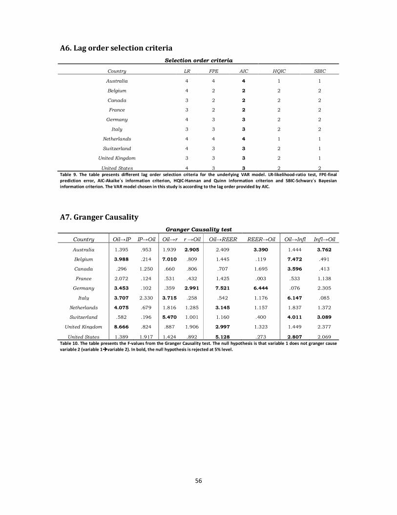
56
A6. Lag order selection criteria
Selection order criteria
Country LR FPE AIC HQIC SBIC
Australia 4 4 4 1 1
Belgium 4 2 2 2 2
Canada 3 2 2 2 2
France 3 2 2 2 2
Germany 4 3 3 2 2
Italy 3 3 3 2 2
Netherlands 4 4 4 1 1
Switzerland 4 3 3 2 1
United Kingdom 3 3 3 2 1
United States 4 3 3 2 2
Table 9. The table presents different lag order selection criteria for the underlying VAR model. LR-likelihood-ratio test, FPE-final
prediction error, AIC-Akaike´s information criterion, HQIC-Hannan and Quinn information criterion and SBIC-Schwarz´s Bayesian
information criterion. The VAR model chosen in this study is according to the lag order provided by AIC.
A7. Granger Causality
Granger Causality test
Country Oil→IP IP→Oil Oil→r r →Oil Oil→REER REER→Oil Oil→Infl Infl→Oil
Australia 1.395 .953 1.939 2.905 2.409 3.390 1.444 3.762
Belgium 3.988 .214 7.010 .809 1.445 .119 7.472 .491
Canada .296 1.250 .660 .806 .707 1.695 3.596 .413
France 2.072 .124 .531 .432 1.425 .003 .533 1.138
Germany 3.453 .102 .359 2.991 7.521 6.444 .076 2.305
Italy 3.707 2.330 3.715 .258 .542 1.176 6.147 .085
Netherlands 4.075 .679 1.816 1.285 3.145 1.157 1.837 1.372
Switzerland .582 .196 5.470 1.001 1.160 .400 4.011 3.089
United Kingdom 8.666 .824 .887 1.906 2.997 1.323 1.449 2.377
United States 1.389 1.917 1.424 .892 5.128 .273 2.807 2.069
Table 10. The table presents the F-values from the Granger Causality test. The null hypothesis is that variable 1 does not granger cause
variable 2 (variable 1����variable 2). In bold, the null hypothesis is rejected at 5% level.

57
-0,006
-0,004
-0,002
0,000
0,002
0,004
0 4 8 12 16
Industrial production
-0,020
-0,010
0,000
0,010
0,020
0 4 8 12 16
Real exchange rate
-0,003
-0,001
0,001
0,003
0 4 8 12 16
Inflation rate
-0,008
-0,004
0,000
0,004
0,008
0 4 8 12 16
Industrial production
-0,004
-0,002
0,000
0,002
0,004
0 4 8 12 16
Real exchange rate
-0,004
-0,002
0,000
0,002
0,004
0 4 8 12 16
Inflation rate
-0,004
-0,002
0,000
0,002
0 4 8 12 16
Real interest rate
-0,004
-0,002
0,000
0,002
0 4 8 12 16
Real interest rate
A8. Impulse Response
Australia
Belgium
Figure 21. The figure presents the orthogonalised impulse-response function of Industrial production, real interest rate, Real
exchange rate and Inflation rate to a one-standard-deviation oil price innovation for Australia and Belgium.

58
-0,010
-0,006
-0,002
0,002
0,006
0 4 8 12 16
Industrial production
-0,008
-0,004
0,000
0,004
0,008
0,012
0 4 8 12 16
Real exchange rate
-0,004
-0,002
0,000
0,002
0,004
0 4 8 12 16
Inflation rate
-0,008
-0,004
0,000
0,004
0,008
0 4 8 12 16
Industrial production
-0,005
-0,003
-0,001
0,001
0,003
0,005
0 4 8 12 16
Real exchange rate
-0,002
-0,001
0,000
0,001
0,002
0,003
0,004
0 4 8 12 16
Inflation rate
-0,002
-0,001
0,000
0,001
0,002
0 4 8 12 16
Real interest rate
-0,003
-0,002
-0,001
0,000
0,001
0,002
0 4 8 12 16
Real interest rate
Canada
France
Figure 22. The figure presents the orthogonalised impulse-response function of Industrial production, real interest rate, Real
exchange rate and Inflation rate to a one-standard-deviation oil price innovation for Canada and France.

59
-0,010
-0,006
-0,002
0,002
0,006
0,010
0 4 8 12 16
Industrial production
-0,008
-0,006
-0,004
-0,002
0,000
0,002
0,004
0 4 8 12 16
Real exchange rate
-0,001
0,000
0,001
0,002
0,003
0 4 8 12 16
Inflation rate
-0,010
-0,006
-0,002
0,002
0,006
0,010
0 4 8 12 16
Industrial production
-0,006
-0,004
-0,002
0,000
0,002
0,004
0 4 8 12 16
Real exchange rate
-0,003
-0,001
0,001
0,003
0,005
0 4 8 12 16
Inflation rate
-0,004
-0,002
0,000
0,002
0 4 8 12 16
Real interest rate
-0,002
-0,001
0,000
0,001
0,002
0 4 8 12 16
Real interest rate
Germany
Italy
Figure 23. The figure presents the orthogonalised impulse-response function of Industrial production, real interest rate, Real
exchange rate and Inflation rate to a one-standard-deviation oil price innovation for Germany and Italy.

60
-0,008
-0,006
-0,004
-0,002
0,000
0,002
0,004
0,006
0 4 8 12 16
Industrial production
-0,006
-0,004
-0,002
0,000
0,002
0,004
0 4 8 12 16
Real exchange rate
-0,001
0,000
0,001
0,002
0,003
0 4 8 12 16
Inflation rate
-0,008
-0,006
-0,004
-0,002
0,000
0,002
0,004
0,006
0 4 8 12 16
Industrial production
-0,008
-0,006
-0,004
-0,002
0,000
0,002
0,004
0,006
0 4 8 12 16
Real exchange rate
-0,002
-0,001
0,000
0,001
0,002
0,003
0 4 8 12 16
Inflation rate
-0,003
-0,002
-0,001
0,000
0,001
0,002
0 4 8 12 16
Real interest rate
-0,002
-0,001
0,000
0,001
0,002
0 4 8 12 16
Real interest rate
Netherlands
Switzerland
Figure 24. The figure presents the orthogonalised impulse-response function of Industrial production, real interest rate, Real
exchange rate and Inflation rate to a one-standard-deviation oil price innovation for Netherlands and Switzerland.

61
-0,006
-0,002
0,002
0,006
0,010
0 4 8 12 16
Industrial production
-0,008
-0,004
0,000
0,004
0,008
0,012
0 4 8 12 16
Real exchange rate
-0,002
0,000
0,002
0,004
0 4 8 12 16
Inflation rate
-0,004
-0,002
0,000
0,002
0 4 8 12 16
Real interest rate
United Kingdom
Figure 25. The figure presents the orthogonalised impulse-response function of Industrial production, real interest rate, Real
exchange rate and Inflation rate to a one-standard-deviation oil price innovation for United Kingdom .

62
A9. Variance decomposition
Country IP r REER Infl
Australia 0,021 0,029 0,074 0,030
(0,96) (1,14) (2,04) (1,17)
Belgium 0,050 0,182 0,011 0,354
(1,56) (2,85) (0,68) (4,47)
Canada 0,013 0,030 0,054 0,154
(0,65) (1,14) (1,54) (2,57)
France 0,090 0,063 0,025 0,236
(2,33) (1,60) (1,10) (3,62)
Germany 0,083 0,024 0,086 0,094
(2,28) (1,08) (2,11) (2,04)
Italy 0,051 0,100 0,006 0,225
(1,83) (2,08) (0,47) (3,37)
Netherlands 0,041 0,082 0,073 0,109
(1,41) (2,08) (1,65) (2,14)
Switzerland 0,019 0,069 0,022 0,091
(1,00) (1,95) (0,90) (2,10)
United Kingdom 0,146 0,044 0,046 0,094
(3,02) (1,19) (1,41) (1,67)
United States 0,059 0,123 0,059 0,264
(1,53) (2,51) (1,70) (4,32)
Table 11. This table presents the results of the estimated variance decomposition at the 4-period horizon (one year).

63
0,00
0,20
0,40
0,60
0,80
1,00
1,20
0,00 0,20 0,40 0,60 0,80 1,00 1,20 1,40 1,60
Australia
1965-78: slope 1.25
1985-95: slope 0.95
1997-10: slope 0.32
0,00
0,20
0,40
0,60
0,80
1,00
1,20
0,00 0,20 0,40 0,60 0,80 1,00 1,20 1,40
Austria
1965-73: slope 1.87
1985-06: slope 0.74
0,00
0,20
0,40
0,60
0,80
0,00 0,20 0,40 0,60 0,80 1,00 1,20 1,40 1,60
Canada
1965-79: slope 0.93
1985-07: slope 0.63
0,00
0,50
1,00
1,50
2,00
2,50
3,00
3,50
4,00
4,50
0,00 0,50 1,00 1,50 2,00 2,50 3,00 3,50 4,00 4,50
China
1968-78: slope 2.29
1984-03: slope 0.70
2004-10: slope 0.46
A10. Oil Consumption and Economic growth
Figure 26. X-axis: cumulative change in natural logarithm of the country´s GDP in 2000s dollars between 1965 and the year for which a given data point is plotted, source: World Bank. Y-axis: cumulative
change in natural logarithm of oil supplied to the country´s market between 1965 and the year for which a given data point is plotted, source BP Statistical Review 2011.
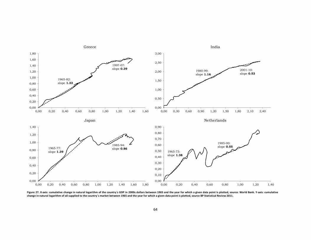
64
0,00
0,50
1,00
1,50
2,00
2,50
3,00
0,00 0,30 0,60 0,90 1,20 1,50 1,80 2,10 2,40
India
1980-99: slope 1.16
2001-10: slope 0.53
0,00
0,20
0,40
0,60
0,80
1,00
1,20
1,40
1,60
1,80
0,00 0,20 0,40 0,60 0,80 1,00 1,20 1,40 1,60
Greece
1965-82: slope 1.33
1997-07: slope 0.39
0,00
0,20
0,40
0,60
0,80
1,00
1,20
1,40
0,00 0,20 0,40 0,60 0,80 1,00 1,20 1,40 1,60 1,80
Japan
1965-77: slope 1.39
1985-94: slope 0.86
0,00
0,10
0,20
0,30
0,40
0,50
0,60
0,70
0,80
0,90
0,00 0,20 0,40 0,60 0,80 1,00 1,20 1,40
Netherlands
1965-73: slope 1.38
1985-00: slope 0.55
Figure 27. X-axis: cumulative change in natural logarithm of the country´s GDP in 2000s dollars between 1965 and the year for which a given data point is plotted, source: World Bank. Y-axis: cumulative
change in natural logarithm of oil supplied to the country´s market between 1965 and the year for which a given data point is plotted, source BP Statistical Review 2011.

65
0,00
0,10
0,20
0,30
0,40
0,50
0,60
0,70
0,80
0,90
1,00
0,00 0,20 0,40 0,60 0,80 1,00 1,20 1,40 1,60
Norway
1974-10: slope 0.42
1965-70: slope 2.00
0,00
0,20
0,40
0,60
0,80
1,00
1,20
1,40
1,60
1,80
2,00
0,00 0,20 0,40 0,60 0,80 1,00 1,20 1,40 1,60
Portugal
1965-00: slope 1.26
0,00
0,30
0,60
0,90
1,20
1,50
1,80
2,10
0,00 0,20 0,40 0,60 0,80 1,00 1,20 1,40 1,60
Spain
1965-76: slope 2.07
1985-05: slope 0.87
-0,10
0,20
0,50
0,80
1,10
1,40
1,70
2,00
2,30
0,00 0,20 0,40 0,60 0,80 1,00 1,20 1,40 1,60 1,80 2,00
Turkey
1967-73: slope 2.63
1975-94: slope 1.05
1995-10: slope 0.06
Figure 28. X-axis: cumulative change in natural logarithm of the country´s GDP in 2000s dollars between 1965 and the year for which a given data point is plotted, source: World Bank. Y-axis: cumulative
change in natural logarithm of oil supplied to the country´s market between 1965 and the year for which a given data point is plotted, source BP Statistical Review 2011.
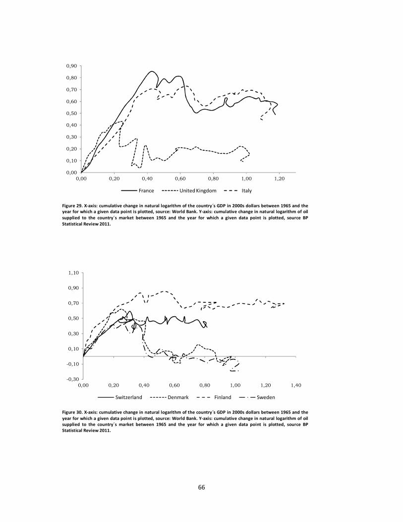
66
0,00
0,10
0,20
0,30
0,40
0,50
0,60
0,70
0,80
0,90
0,00 0,20 0,40 0,60 0,80 1,00 1,20
France United Kingdom Italy
-0,30
-0,10
0,10
0,30
0,50
0,70
0,90
1,10
0,00 0,20 0,40 0,60 0,80 1,00 1,20 1,40
Switzerland Denmark Finland Sweden
Figure 29. X-axis: cumulative change in natural logarithm of the country´s GDP in 2000s dollars between 1965 and the
year for which a given data point is plotted, source: World Bank. Y-axis: cumulative change in natural logarithm of oil
supplied to the country´s market between 1965 and the year for which a given data point is plotted, source BP
Statistical Review 2011.
Figure 30. X-axis: cumulative change in natural logarithm of the country´s GDP in 2000s dollars between 1965 and the
year for which a given data point is plotted, source: World Bank. Y-axis: cumulative change in natural logarithm of oil
supplied to the country´s market between 1965 and the year for which a given data point is plotted, source BP
Statistical Review 2011.

67
A11. Countries Energy Mix
Australia Oil Gas Coal Nuclear Hydro Renew. Austria Oil Gas Coal Nuclear Hydro Renew. Canada Oil Gas Coal Nuclear Hydro Renew.
1965-72 0,52 0,02 0,41 .. 0,05 .. 1965-72 0,43 0,12 0,22 .. 0,22 .. 1965-72 0,46 0,20 0,11 0,00 0,23 ..
1973-80 0,48 0,11 0,36 .. 0,05 .. 1973-80 0,47 0,17 0,13 .. 0,22 .. 1973-80 0,43 0,22 0,09 0,03 0,23 ..
1981-89 0,39 0,17 0,40 .. 0,04 .. 1981-89 0,40 0,18 0,13 .. 0,28 .. 1981-89 0,33 0,22 0,11 0,06 0,28 ..
1990-99 0,36 0,17 0,43 .. 0,04 0,00 1990-99 0,39 0,23 0,10 .. 0,27 0,01 1990-99 0,30 0,26 0,10 0,07 0,27 0,00
2000-10 0,34 0,19 0,43 .. 0,03 0,01 2000-10 0,40 0,25 0,08 .. 0,24 0,03 2000-10 0,31 0,27 0,10 0,06 0,26 0,01
China Oil Gas Coal Nuclear Hydro Renew. Denmark Oil Gas Coal Nuclear Hydro Renew. Finland Oil Gas Coal Nuclear Hydro Renew.
1965-72 0,13 0,01 0,83 .. 0,03 .. 1965-72 0,88 .. 0,12 .. 0,00 .. 1965-72 0,66 .. 0,16 .. 0,18 ..
1973-80 0,22 0,03 0,72 .. 0,03 .. 1973-80 0,83 .. 0,17 .. 0,00 .. 1973-80 0,67 0,03 0,14 0,03 0,13 ..
1981-89 0,18 0,02 0,76 .. 0,04 .. 1981-89 0,60 0,04 0,36 .. 0,00 .. 1981-89 0,50 0,04 0,13 0,19 0,14 ..
1990-99 0,19 0,02 0,75 0,00 0,04 0,00 1990-99 0,49 0,15 0,33 .. 0,00 0,02 1990-99 0,41 0,11 0,14 0,18 0,11 0,06
2000-10 0,20 0,03 0,71 0,01 0,06 0,00 2000-10 0,46 0,22 0,22 .. 0,00 0,10 2000-10 0,37 0,12 0,15 0,18 0,10 0,07
France Oil Gas Coal Nuclear Hydro Renew. Greece Oil Gas Coal Nuclear Hydro Renew. India Oil Gas Coal Nuclear Hydro Renew.
1965-72 0,57 0,06 0,29 0,01 0,08 .. 1965-72 0,67 .. 0,28 .. 0,05 .. 1965-72 0,28 0,01 0,61 0,00 0,10 ..
1973-80 0,63 0,11 0,16 0,03 0,07 .. 1973-80 0,63 .. 0,33 .. 0,04 .. 1973-80 0,30 0,01 0,57 0,01 0,11 ..
1981-89 0,45 0,12 0,11 0,24 0,08 .. 1981-89 0,66 0,00 0,30 .. 0,04 .. 1981-89 0,31 0,03 0,56 0,01 0,09 ..
1990-99 0,39 0,13 0,07 0,35 0,06 0,00 1990-99 0,65 0,01 0,31 .. 0,03 .. 1990-99 0,32 0,07 0,52 0,01 0,07 0,00
2000-10 0,36 0,15 0,05 0,38 0,05 0,01 2000-10 0,62 0,08 0,26 .. 0,03 0,01 2000-10 0,33 0,09 0,51 0,01 0,06 0,01
Italy Oil Gas Coal Nuclear Hydro Renew. Japan Oil Gas Coal Nuclear Hydro Renew. Netherland Oil Gas Coal Nuclear Hydro Renew.
1965-72 0,71 0,10 0,09 0,01 0,10 .. 1965-72 0,67 0,01 0,24 0,00 0,08 .. 1965-72 0,66 0,19 0,15 0,00 .. ..
1973-80 0,71 0,14 0,07 0,01 0,07 .. 1973-80 0,74 0,03 0,15 0,03 0,05 .. 1973-80 0,52 0,43 0,04 0,01 .. ..
1981-89 0,63 0,20 0,10 0,01 0,06 .. 1981-89 0,59 0,09 0,19 0,09 0,05 .. 1981-89 0,46 0,44 0,09 0,01 .. ..
1990-99 0,58 0,28 0,07 .. 0,06 0,01 1990-99 0,54 0,11 0,18 0,13 0,04 0,01 1990-99 0,46 0,42 0,11 0,01 .. 0,00
2000-10 0,48 0,36 0,09 .. 0,05 0,02 2000-10 0,46 0,14 0,22 0,13 0,04 0,01 2000-10 0,51 0,38 0,09 0,01 .. 0,02
Table 12. Average energy mix share. Source BP Statistical Review 2011.

68
Norway Oil Gas Coal Nuclear Hydro Renew. Portugal Oil Gas Coal Nuclear Hydro Renew. Spain Oil Gas Coal Nuclear Hydro Renew.
1965-72 0,33 .. 0,05 .. 0,62 .. 1965-72 0,68 .. 0,10 .. 0,23 .. 1965-72 0,61 0,00 0,22 0,01 0,17 ..
1973-80 0,32 0,01 0,02 .. 0,65 .. 1973-80 0,75 .. 0,05 .. 0,20 .. 1973-80 0,69 0,02 0,15 0,02 0,11 ..
1981-89 0,26 0,04 0,01 .. 0,69 .. 1981-89 0,74 .. 0,09 .. 0,17 .. 1981-89 0,58 0,03 0,23 0,08 0,08 ..
1990-99 0,25 0,07 0,01 .. 0,67 0,00 1990-99 0,68 0,01 0,18 .. 0,12 0,01 1990-99 0,55 0,08 0,18 0,12 0,06 0,00
2000-10 0,23 0,09 0,01 .. 0,66 0,00 2000-10 0,58 0,13 0,14 .. 0,10 0,05 2000-10 0,52 0,17 0,12 0,09 0,05 0,04
Sweden Oil Gas Coal Nuclear Hydro Renew. Switzerland Oil Gas Coal Nuclear Hydro Renew. Turkey Oil Gas Coal Nuclear Hydro Renew.
1965-72 0,67 .. 0,04 0,00 0,30 .. 1965-72 0,60 0,00 0,04 0,01 0,35 .. 1965-72 0,59 .. 0,36 .. 0,06 ..
1973-80 0,60 .. 0,04 0,08 0,29 .. 1973-80 0,58 0,02 0,01 0,08 0,30 .. 1973-80 0,67 .. 0,26 .. 0,08 ..
1981-89 0,39 0,00 0,05 0,25 0,31 .. 1981-89 0,47 0,05 0,01 0,17 0,30 .. 1981-89 0,54 0,01 0,34 .. 0,10 ..
1990-99 0,33 0,01 0,04 0,31 0,30 0,01 1990-99 0,45 0,07 0,01 0,19 0,27 0,01 1990-99 0,45 0,10 0,33 .. 0,12 0,00
2000-10 0,31 0,02 0,04 0,29 0,30 0,04 2000-10 0,42 0,09 0,00 0,21 0,27 0,01 2000-10 0,34 0,26 0,30 .. 0,09 0,00
United Kingdom Oil Gas Coal Nuclear Hydro Renew. United States Oil Gas Coal Nuclear Hydro Renew.
1965-72 0,45 0,04 0,48 0,03 0,00 .. 1965-72 0,43 0,33 0,20 0,00 0,04 ..
1973-80 0,45 0,16 0,35 0,04 0,00 .. 1973-80 0,46 0,29 0,19 0,03 0,04 ..
1981-89 0,39 0,22 0,32 0,06 0,01 .. 1981-89 0,41 0,26 0,24 0,05 0,04 ..
1990-99 0,38 0,29 0,23 0,09 0,00 0,00 1990-99 0,38 0,26 0,24 0,07 0,03 0,01
2000-10 0,36 0,38 0,16 0,08 0,00 0,01 2000-10 0,39 0,25 0,24 0,08 0,03 0,01
Table 13. Average energy mix share. Source BP Statistical Review 2011.
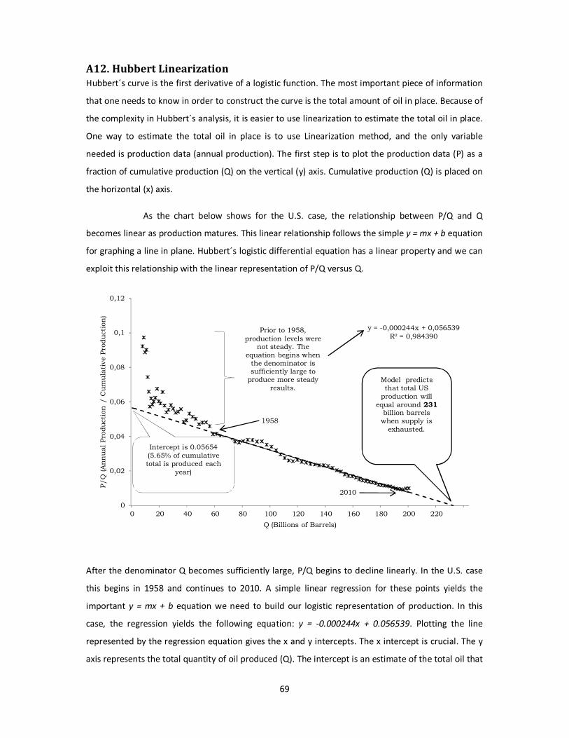
69
y = -0,000244x + 0,056539R² = 0,984390
0
0,02
0,04
0,06
0,08
0,1
0,12
0 20 40 60 80 100 120 140 160 180 200 220
P/Q (Annual Production / Cumulative Production)
Q (Billions of Barrels)
Intercept is 0.05654(5.65% of cumulative total is produced each
year)
Prior to 1958,production levels were
not steady. The equation begins when the denominator is sufficiently large to produce more steady
results.Model predictsthat total US production will
equal around 231billion barrels when supply is exhausted.
1958
2010
A12. Hubbert Linearization
Hubbert´s curve is the first derivative of a logistic function. The most important piece of information
that one needs to know in order to construct the curve is the total amount of oil in place. Because of
the complexity in Hubbert´s analysis, it is easier to use linearization to estimate the total oil in place.
One way to estimate the total oil in place is to use Linearization method, and the only variable
needed is production data (annual production). The first step is to plot the production data (P) as a
fraction of cumulative production (Q) on the vertical (y) axis. Cumulative production (Q) is placed on
the horizontal (x) axis.
As the chart below shows for the U.S. case, the relationship between P/Q and Q
becomes linear as production matures. This linear relationship follows the simple y = mx + b equation
for graphing a line in plane. Hubbert´s logistic differential equation has a linear property and we can
exploit this relationship with the linear representation of P/Q versus Q.
After the denominator Q becomes sufficiently large, P/Q begins to decline linearly. In the U.S. case
this begins in 1958 and continues to 2010. A simple linear regression for these points yields the
important y = mx + b equation we need to build our logistic representation of production. In this
case, the regression yields the following equation: y = -0.000244x + 0.056539. Plotting the line
represented by the regression equation gives the x and y intercepts. The x intercept is crucial. The y
axis represents the total quantity of oil produced (Q). The intercept is an estimate of the total oil that
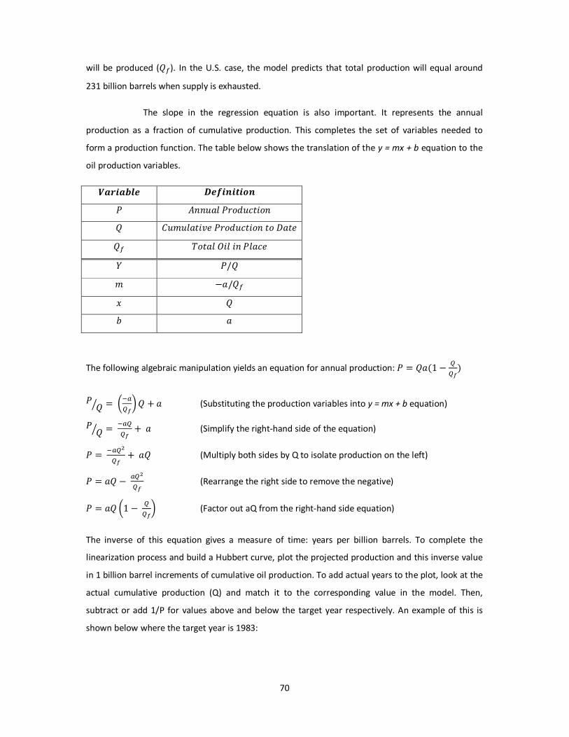
70
will be produced (YZ). In the U.S. case, the model predicts that total production will equal around
231 billion barrels when supply is exhausted.
The slope in the regression equation is also important. It represents the annual
production as a fraction of cumulative production. This completes the set of variables needed to
form a production function. The table below shows the translation of the y = mx + b equation to the
oil production variables.
[\]^\_`a bac^d^e^fd ( g����� (��h���0�� Y 5�i����0j� (��h���0�� �� A���
YZ ����� '0� 0� (���� L (/Y i "�/YZ
T Y W �
The following algebraic manipulation yields an equation for annual production: ( � Y��1 " kkl
�
( Ym � n#okl
p Y 6 � (Substituting the production variables into y = mx + b equation)
( Ym � #okkl
6 � (Simplify the right-hand side of the equation)
( � #okqkl
6 �Y (Multiply both sides by Q to isolate production on the left)
( � �Y " okqkl
(Rearrange the right side to remove the negative)
( � �Y n1 " kkl
p (Factor out aQ from the right-hand side equation)
The inverse of this equation gives a measure of time: years per billion barrels. To complete the
linearization process and build a Hubbert curve, plot the projected production and this inverse value
in 1 billion barrel increments of cumulative oil production. To add actual years to the plot, look at the
actual cumulative production (Q) and match it to the corresponding value in the model. Then,
subtract or add 1/P for values above and below the target year respectively. An example of this is
shown below where the target year is 1983:
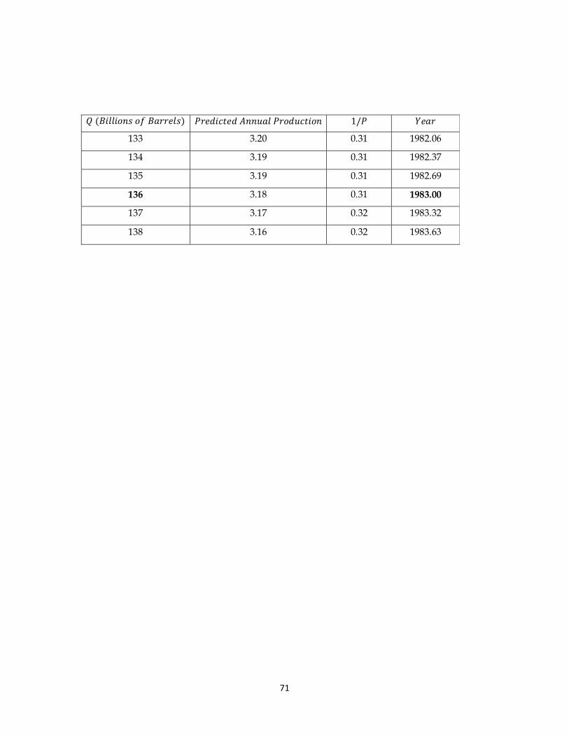
71
Y �r0��0��s �U r�����s� (��h0���h g����� (��h���0�� 1/( L���
133 3.20 0.31 1982.06
134 3.19 0.31 1982.37
135 3.19 0.31 1982.69
136 3.18 0.31 1983.00
137 3.17 0.32 1983.32
138 3.16 0.32 1983.63

72
0,00
0,20
0,40
0,60
0,80
1,00
1,20
1,40
1960 1980 2000 2020 2040 2060 2080
Billion barrels/year
Actual production
Model prediction
In 2010, Canada had produced 39 percent of its total expected output (96 billion
barrels). The peak is expected to be reached around
2020?.
0,00
0,20
0,40
0,60
0,80
1,00
1,20
1,40
1,60
1960 1980 2000 2020 2040
Billion barrels/year
Actual production
Model prediction
In 2010, Mexico had produced 69 percent of its total expected
output (58 billion barrels). Actual peak was reached in 2003. Model peak in 2000.
Hubbert Curve: Canada and Mexico

73
0,00
0,20
0,40
0,60
0,80
1,00
1,20
1,40
1970 1980 1990 2000 2010 2020 2030
Billion barrels/year
Actual production
Model prediction
In 2010, Norway had produced 83 percent of its total expected output (30 billion barrels).
Actual peak was reached in 2000. Model peak in
2000.
0,00
0,20
0,40
0,60
0,80
1,00
1,20
1960 1980 2000 2020 2040
Billion barrels/year
Actual production
Model prediction
In 2010, U.K. had produced 87 percent of
its total expected output (31 billion
barrels). Actual peak was reached in 1999. Model peak in 1994.
Hubbert Curve: Norway and UK

74
0,00
0,20
0,40
0,60
0,80
1,00
1,20
1,40
1,60
1960 1980 2000 2020 2040 2060
Billion barrels/year
Actual production
Model prediction
In 2010, China had produced 52 percent of its total
expected output (77 billion barrels). Actual peak was reached in 2008 or 2010?.
Model peak in 2008.
0,00
0,05
0,10
0,15
0,20
0,25
0,30
0,35
1960 1980 2000 2020 2040
Billion barrels/year
Actual production
Model prediction
In 2010, India had produced 65 percent of its total expected output (13 billion barrels).
Actual peak was reached in 2010. Model peak
around 2005.
Hubbert Curve: China and India

75
0,00
0,10
0,20
0,30
0,40
0,50
0,60
0,70
1950 1970 1990 2010 2030
Billion barrels/year
Actual production
Model prediction
In 2010, Indonesia had produced 83 percent of its total expected output (26 billion barrels). Actual peak was reached in 1977.
Model peak in 1990.
0,00
0,05
0,10
0,15
0,20
0,25
0,30
0,35
1960 1970 1980 1990 2000 2010 2020 2030
Billion barrels/year
Actual production
Model prediction
In 2010, Australia had produced 74 percent of its total expected output (11
billion barrels). Actual peak was reached in 2000. Model
peak around 1996.
Hubbert Curve: Indonesia and Australia

76
0,00
0,50
1,00
1,50
2,00
2,50
3,00
3,50
4,00
4,50
1950 1970 1990 2010 2030 2050 2070
Billion barrels/year
Actual production
Model prediction
In 2010, Saudi Arabia had produced 59 percent of its total expected output (216 billion barrels). Actual peak was
reached in 2005?. Model peak around 2005.
0,00
0,20
0,40
0,60
0,80
1,00
1,20
1950 1970 1990 2010 2030 2050
Billion barrels/year
Actual production
Model prediction
In 2010, UAE had produced 59 percent of its total expected output (55 billion barrels). Actual peak was reached in
2006?. Model peak around 2004.
Hubbert Curve: Saudi Arabia and UAE

77
Hubbert Curve: World
0,00
5,00
10,00
15,00
20,00
25,00
30,00
1900 1950 2000 2050 2100
Billion barrels/year
Model prediction
Actual production
In 2010, the World had produced 59 percent of its total expected output (1805 billion barrels). Actual peak was reached around 2010?. Model
peak around 2003.

78
A13. Some geopolitical and other
aspects
Pre 1973- The fall of Bretton Woods
In the 1950s and 1960s, almost every currency in
the world was anchored to the U.S. dollar and the
dollar in turn was anchored to gold ($35 per
ounce). In the late 1960s, the United States was
running balance of payments deficits and trade
deficits following the costs of the Vietnam War and
increased domestic spending which accelerated
inflation. The effect of the expansionary monetary
policy in the United States, and the associated rise
in inflation was a depreciation of the dollar´s real
exchange rate, or a real appreciation of other
countries currencies. Other countries tried to resist
this appreciation pressures by buying dollars. The
dollar reserves for those countries accumulated
and inflationary pressures grew as those countries
supplied more of their own currencies to the
foreign exchange markets in order to keep their
currencies pegged to the dollar at the fixed rates.
Therefore, they accused the U.S. of “exporting”
inflation, Hammes and Wills (2005).
When those countries started to
redeem their dollar reserves for gold, it became
clear that the United States could no longer hold
the gold price of $35 per ounce. In order to slow
the outflow of gold, the United States suspended
its obligation to buy dollars from foreign central
banks at $35 per ounce and on August 7 1971,
Richard Nixon closed the “gold window”. With the
“floating” of gold, the world moved from a fixed to
a flexible exchange rate system as more countries
stopped interventions in the foreign exchange
market once the United States stopped buying
dollars with gold, Hammes and Wills (2005). Gold
price was initially revalued to $38, by the end of
the 1970s it had risen to more than $450, i.e. an
increase of 1084 percent in a decade (Figure 31).
The value of the dollar declined on
average 20 percent against major currencies
(Figure 13) during the period 1971-1973. Given
that oil contracts were in US dollars, the declining
value of the dollar meant less revenue for OPEC
per unit (barrel) sold to most western countries. To
give a glimpse of OPECs loss during this period, one
can think of oil priced in gold (T.Ounce/barrel).
From figure 32, we can observe that 4 months
before the closing of the “gold window” one barrel
equaled 0.07 T.Ounce of gold, that is to say, to buy
1 T.Ounce of gold, OPEC had to pay approximately
14 barrels of oil. By October 1972 (one year before
OPEC embargo), OPEC had to pay 25 barrels per
T.Ounce of gold. The decline in “real” price of oil
and the general worldwide inflation did not go
unnoticed by OPEC member countries.
In response to the declining value
of the dollar, OPEC member countries agreed (the
Tehran Agreement of 1971) on an 8.25 percent
increase in the price of oil which corresponded to
the rise of 8.57 percent in the price of gold vis-á-vis
the US dollar. At the same meeting they also
agreed on that the future price of oil would be
adjusted on a quarterly basis in line with an index
based on the movements of nine major
industrialized nations28
vis-á-vis the US dollar,
Ahrari (1986). Yet, by July 1973, nearly 40 barrels
was required to buy 1 T.Ounce of gold. This
automatic indexing was abandoned short after
October 1973.
28
Britain, France, West Germany, Italy, Japan, Belgium,
Holland, Sweden and Switzerland.

79
0
20
40
60
80
100
120
140
0
200
400
600
800
1 000
1 200
1 400
1971 1976 1981 1986 1991 1996 2001 2006 2011
$US/Barrel
$US/T.Ounce
Gold Price ($US/T.Ounce) Crude Oil Price ($US/Barrel)
0,02
0,04
0,06
0,08
0,1
0,12
0,14
0,16
1971 1976 1981 1986 1991 1996 2001 2006 2011
T.Ounce/Barrel
Gold Price of Crude Oil (T.Ounce/Barrel)
Average: 0.06962
Figure 32. Dollar prices of gold and oil 1971 January- 2011 May. Source: International Financial Statistics (world oil price) and IHS Global Insight (Gold Price).
Figure 31. Gold price of crude oil 1971 January- 2011 May (troy ounces/barrel). Source: International Financial Statistics (world oil price) and HIS Global Insight (Gold Price).

80
-8%
-6%
-4%
-2%
0%
2%
Sep-73
Oct-73
Nov-73
Dec-73
Jan-74
Feb-74
Mar-74
Apr-74
May-74
Jun-74
Jul-74
Aug-74
Sep-74
OPEC World Non-OPEC
1973-1974: The October War and the Oil
Embargo
By 1973, the Bretton Woods monetary system was
dead. The October War was part of the Arab-Israel
conflict which was ongoing from 1948 when the
state of Israel was formed. It was the fourth Arab-
Israeli War which was led by Egypt and Syria and
started with a surprising attack on Israel on Yom
Kippur the holiest day in Judaism, which coincided
with the Muslim holy month of Ramadan. The war
was fought from October 6 to October 25 in 1973.
In response to the U.S. decision to resupply the
Israeli military, the OPEC plus other Arab countries
announced on October 16 that they would cut
supply of oil by 5%
“Until the Israeli forces are completely evacuated
from all the Arab territories occupied
In the June 1967 war and the legitimate rights of
the Palestinian people are restored.”29
Below in figure 33, I have plotted the change in
production from OPEC, non-OPEC and World
during the months post the October War and the
oil embargo as percentage of total world
production prior to this event. As we can see from
the Figure, the increase in non-OPEC production
was rather minor during this crisis as will be
compared to later crisis below. The immediate
effect of the embargo was that oil price climbed
from an average of $3.00 per barrel prior to the
embargo to $12.00 per barrel in October. This
increase in price had a dramatic effect on oil
exporting countries in the Middle East who had
long been dominated by industrial powers who
now seen to have acquired the power to control
price over a vital commodity.
29
Quotation taken from OPEC ministers´ press release
reported by Al-Sowayegh (1984, p. 129)
This power, to control oil prices and supply became
to be known as the “oil weapon” used by Arab
countries to select industrialized countries as a tool
to put pressure on Israel during the October War,
Licklider (1988). For the U.S. case, the embargo
threatened its energy security as being the largest
oil consuming country in the world. The embargo
left many U.S. oil producers searching for new
ways to develop expensive oil. The major problems
these producers were facing was that; finding oil
and developing new oil fields usually require a time
lag of 5 to 10 years between the planning process
and production, Ikenberry (1986). Another factor
that exacerbated the crisis was U.S. price controls
which were intended to promote oil explorations
through limiting the price of old oil that already
been discovered while allowing newly discovered
oil to be sold at higher price, Helbling and Turley
(1975). This rule also discouraged alternative
energies from being developed. The rule had been
intended to promote oil exploration. The scarcity
of oil was dealt by the rationing of gasoline (which
occurred also in many other European countries),
with motorist facing long lines at gas stations
Fraum (2000).
Japan on the other hand was quick
on taking advantage of the embargo. The auto
makers in Japan also took advantage of the
embargo when realizing the increase in fuel prices
Figure 33. Supply disruption during OPECs embargo. Source:
BP statistical review 2011.

81
in the U.S. They started to produce small, more
fuel efficient models, which they in turn sold to the
U.S. market as an alternative to American “gas-
guzzling” cars of that time. This in turn led to a
drop in American auto sales that lasted into the
1980s.
The effects of the embargo on
Europe were not uniform. Netherlands faced a
complete embargo, United Kingdom and France
was not much affected (having refused to allow the
Americans to use their airfields and embargoed
arms and supplies to both Arabs and Israelis), while
other faced only partial cutbacks. For instance, the
United Kingdom, Germany, Italy, Switzerland and
Norway banned flying, driving and boating on
Sundays. Sweden rationed its gasoline and heating
oil. The Netherlands imposed prison sentences for
those who used more than their given ratio of
electricity use Fraum (2000).
The sudden ability of OPEC to
exercise power in 1973 cannot be explained on the
basis of Arab nationalism alone or the “oil
weapon”. Other factors need to be considered in
order to understand this “sudden ability”. The
global supply and demand for oil were very
important contributing factors. In the background,
there was increase in demand for energy as the
world economy reintegrated and enjoyed one of its
longest periods of economic growth after World
War II. Increase in demand initially prompted
regulators in the U.S., such as Texas Rail
Commission, to eliminate all restrictions on
productions. As Texas was producing the maximum
that it possibly could produce from its field, no
excess capacity remained as backup to be brought
to the market in case of supply shortage
emergency. This in turn eliminated the U.S. role as
being a stabilizing force in global oil market. The
other factor was the trend toward nationalization
of oil resources and the loss of market power of
large multinational oil companies, generally known
as the “seven sisters” which gave OPEC an
oligopolistic power to determine oil prices directly,
El-Gamal and M. Jaffe (2010).
Using the “oil weapon” to put
pressure on the U.S. and the West could off course
be considered as a nationalistic aspect. However, it
is not clear whether these political considerations
could have dominated the oil exporting countries´
economic self interest. In early 1974, Secretary of
State Henry Kissinger announced after a series of
discussions with oil exporting Arab countries that
the use of petroleum as a weapon to influence the
outcome of the Arab-Israeli conflict had little merit
in reality30
. In fact, some supply disruptions
unrelated to the conflict appear to have
contributed significantly to the oil shock of 1973-
7431
. Meanwhile, Saudi Arabia was secretly selling
oil to the U.S. military to help fuel America´s
operations for the Vietnam War, even as it was
publicly announcing its oil sale boycott of America
in solidarity to the Arab cause, Bronson (2006).
30
Department of State, Bulletin 70, no. 1806, 14 February
1974, p. 109- cited in El-Gamal and M. Jaffe (2010, p. 26). 31
Testimony of the Chief Reservoir Engineer of Socal before the
Church Committee, cited in Arhnacarry , p. “The Petroleum
Crisis, Saudi Arabia and U.S. Foreign Policy,” Energy Information
Services 3, 14 April 1981, p.3, suggests that technical problems
in the Shedgum section of the Ghawar field was a significant
cause of supply disruptions.

82
-10%
-8%
-6%
-4%
-2%
0%
2%
4%
Oct-78
Nov-78
Dec-78
Jan-79
Feb-79
Mar-79
Apr-79
May-79
Jun-79
Jul-79
Aug-79
Sep-79
Oct-79
Iran World
OPEC Non-OPEC
Summary
• OPEC announces on October 6 1973 a
production cut of 5 percent and impose
embargo on countries supporting Israel
during October War.
• Oil price rose from $3.42 in September
1973 to $13.43 in January 1974, a 293
percent increase.
• The OPEC embargo knocked 7.0 percent
of world production prior to embargo.
(September 1973-November 1973)
• Price controls exacerbated the crises.
• The effect on Europe was not uniform.
• Other background factors need to be
considered such as the increasing demand
for energy after World War II, elimination
of restriction on production (Texas Rail
Commission), the lost in market power of
big multinational oil companies, the
power of “oil-weapon” and the U.S. and
Saudi Arabia´s thick foreign relations in
order to understand the full scale of the
1973-74 crisis.
1979: The Iranian Revolution
The second oil crisis, the crisis of 1979, occurred in
the wake of the Iranian Revolution. Massive
protests on the Shah of Iran and his western
democratic vision of Iran resulted his fall in the
early 1979. These protests severely disrupted the
supply of Iranian oil, with production being greatly
decreased and exports suspended. In September
1978, Iran produced 6.1 million barrels per day, by
January 1979 production was down to 0.73 million
barrels per day. Oil exports were later resumed
under the new regime; however production was
only 75 percent of that produced prior to the fall of
the Shah which further pushed prices up. To
compensate for the shortfall, Saudi Arabia and
other OPEC members increased their production
and the overall loss in world production was about
4 percent. Below in Figure 34, I have plotted the
change in production from Iran, OPEC, non-OPEC
and World during the months post the Iranian
Revolution as percentage of total world production
prior to the Revolution.
At the same time, the panic in the U.S. was
widespread. In April 1979, President Jimmy Carter
began a phased deregulation of oil prices. At the
time, average oil price was $15.85 per barrel.
Deregulating domestic oil price controls allowed
U.S. oil output to rise sharply from the Prudhoe
Bay fields, although oil imports fell sharply. Long
lines once again appeared at gas stations, just as
they did in 1973. In November 1979, a group of
Iranian students stormed the U.S. Embassy in
Tehran demanding the return of Iran´s deposed
leader, The Shah, who was receiving treatment for
his cancer in the U.S. This action resulted in that
President Jimmy Carter ordering a complete
embargo on Iranian oil which further pushed oil
prices up32
.
32
http://www.history.com/this-day-in-history/iranian-
students-storm-us-embassy-in-tehran-leading-to-oil-embargo
Figure 34. Supply disruptions during The Iranian Revolution.
Source: BP statistical Review 2011.

83
-10%
-8%
-6%
-4%
-2%
0%
2%
Sep-80
Oct-80
Nov-80
Dec-80
Jan-81
Feb-81
Mar-81
Apr-81
May-81
Jun-81
Jul-81
Aug-81
Sep-81
Iran+Iraq World
OPEC Non-OPEC
Summary
• The Iranian Revolution leads to the fall of
the Shah and the Shah flees the country at
end of 1979.
• Oil price rose from $14.05 in December
1978 to $39.7 in November 1979, a 183
percent increase.
• The Iranian Revolution knocked 8.6
percent of world production prior to the
Revolution (September 1978-January
1979).
• A group of Iranian students storms the
U.S. Embassy in Tehran leading to a U.S.
embargo on imports from Iran.
• President Jimmy Carter begins a phase of
deregulation of oil prices in the U.S.
1980: Iraq-Iran war
During the 1970s, the Bathist team of Hasan Al-
Bakr and Saddam Hussein navigated a series of
challenges from without: Syria to the West and
Iran to the East, as well as from within: Kurdish
independence movements in the North and Shiite
political dissent in the south. Those challenges
were navigated through a series of diplomatic
moves (such as the treaty with Iran in 1975),
military threats (such as amassing troops on the
Syrian border), and direct persecution of Kurds in
the North and Shiites in the South. According to
one report, Iraq spent 40 percent of its massive
petrodollar inflows during that period on
weaponry, Tripp (2000) and Pollack (2004).
However, the greatest challenge to the Bathist
regime was posed by the success of the Iranian
revolution (in establishing a religious Shiite state to
its east). The direct and inspirational support from
the revolution in Iran emboldened the Iraqi Shiites
which prompted Saddam Hussein to expel tens of
thousands of Iraqi Shiites that were considered by
the regime to be “Iranian Shiites”. Shortly
thereafter, Saddam Hussein started the first of two
disastrous wars by invading Iran in 1980.
What Saddam Hussein had
envisioned as a minor exercise of power turned
into a devastating eight year long war, as Iran
sought to reassert its presence and to defend the
success of its revolution. Several attacks between
Iran and Iraq on each others´ cities and oil
resources eventually tipped the scales in Iraq´s
favor, as Western powers (especially the U.S.)
moved into the region to protect oil supplies.
Below in Figure 35, we can see the supply
disruptions due to the Iraq-Iran War.
In September 1980 Iraq and Iran were producing
4.0 million barrels per day (1.2 million from Iran
and 2.8 million from Iraq), by October 1980, the
same figure was down to 0.7 million barrels per
day (0.5 million from Iran and 0.2 million from
Iraq).
Financial support from Saudi Arabia and Kuwait,
and military support from both the Soviet Union
and the U.S., eventually forced a cease fire on Iran
in 1988. At the beginning of the war, Iraq held a
clear advantage in armor, while both countries
were roughly equal regarding artillery. The gap
started too widened as the war went on (Table 14).
Figure 35. Supply disruptions during Iraq-Iran War. Source: BP
statistical Review 2011.

84
Iran started with a stronger air force, but over
time, the balance shifted towards favoring Iraq.
The Iraqi economy was devastated from the long
war, which exhausted the bulk of its Dollar
reserves accumulated during the 1970s, and
shackled it with a debt repayment that consumed
50 percent of its oil revenues in 199033
. Total
estimated debt to other countries was $130 billion,
of which $21 billion was borrowed from the Paris
Club34
and the larger portion of the debt was
borrowed from neighboring Arab countries35
.
Summary
• Saddam Hussein sees an opportunity after
the Iranian Revolution to attack the weak
neighboring country Iran after its
Revolution, with the vision of making Iraq
a super power in the region. The war
lasted from September 1980 to August
1988.
• Oil price rose from $31.88 in August 1980
to $40.97 in November 1980, a 29 percent
increase.
33
Foreign currency reserves fell from $30 billion in 1980 to $3
billion in 1983. In 1983 Iraq´s debt had reached $25 billion
(ibid., p. 235). More accurate data on Iraq´s economy and
finances under the Bathist rule are not available, because they
were treated as state secrets, (ibid. p. 214). 34
This debt was originated from Japan, Russia, France,
Germany, United States, Italy and the United Kingdom. 35
The large portion of the debt was from Kuwait, Saudi Arabia,
Qatar, UAE and Jordan.
• The war knocked 7.2 percent of world
production prior to the war (July 1980-
October 1980).
• Many countries were supporting both Iraq
and Iran through the war period, though
the support favored Iraq.
• Iraq ends up with a $130 billion debt for
financing the war.
The Price Collapse of 1980s
In the early 1980 there was a serious surplus of
crude oil caused by falling demand following the
crisis in 1973 and 1979. World oil price was
peaking at $40.97 per barrel (nominal terms) in
November 1980. From that peak, price started to
decline gradually and in the first half of 1986 price
fell from $26.75 per barrel in December 1985 to
$9.88 per barrel in July 1986. The surplus of oil
began in the early 1980s as a result of slowed
economic activity in industrial countries and the
energy conservation spurred by high fuel prices36
.
Figure 36 presents oil consumption in Europe,
Japan and the United States and production of
OPEC, non-OPEC and Former Soviet Union (Figure
37) during the period 1965 to 1990.
36
Oil Glut, Price Cuts: How Long Will They Last?". 89. U.S. News
& World Report. 1980-08-18. p. 44.
Table 14. Military strength of Iraq and Iran during the War.
Source: "The Arming, and Disarming, of Iran's Revolution," The
Economist, International Edition, 19 September 1987, 56-57.
Imbalance of Power (1980-87) Iraq Iran
Tanks in 1980 2700 1740
Tanks in 1987 4500+ 1000
Fighter Aircraft in 1980 332 445
Fighter Aircraft in 1987 500+ 65
Helicopters in 1980 40 500
Helicopters in 1987 150 60
Artillery in 1980 1000 1000+
Artillery in 1987 4000+ 1000+

85
02 0004 0006 0008 00010 00012 00014 00016 00018 00020 000
1965
1967
1969
1971
1973
1975
1977
1979
1981
1983
1985
1987
1989
Europe Japan
United States
0
5 000
10 000
15 000
20 000
25 000
30 000
35 000
1965
1967
1969
1971
1973
1975
1977
1979
1981
1983
1985
1987
1989
Soviet Union OPEC
Non-OPEC
Consumption had fallen with 17 percent, 19
percent and 15 percent from 1979 to 1985 for
Europe, Japan and United States respectively. This
falling demand in combination with
overproduction from non-OPEC (Figure 37) caused
the six-year long decline in oil prices37
.
The remove of market controls from petroleum
products in the late 1970s, which allowed the free
market to adjust oil prices in the United States,
encouraged oil producers in the United States to
increase production. The United States Oil Windfall
37
http://www.nytimes.com/2008/03/03/business/worldbusines
s/03cnd-oil.html?hp
profits tax38
was lowered in August 1981 and
removed in 1988, ending disincentives to oil
producers in the United States39
. The United States
import of crude oil fell from 46.5 percent in 1977
to 28 percent in 1982 and 1983 due to lower
consumption. The reliance on Middle East source
dwindled even further as United Kingdom, Mexico
Nigeria and Norway joined Canada in the forefront
of American suppliers40
.
From 1979 to 1986, OPEC
decreased its production several times in an
attempt to keep oil prices high. OPEC production
fell from 30 million bpd in 1979 to 15.9 million bpd
in 1985, i.e. a decrease with approximately 50
percent. However, OPEC failed to hold on to its
preeminent position and by 1981 its production
was surpassed by Non-OPEC production. OPEC
share of total world production fell from 51
percent in the mid 1970s to 28 percent in 1985.
OPEC´s membership began to have divided
opinions over what actions to take. In September
1985, Saudi Arabia tried to gain market share by
increasing production, creating a “huge surplus
that angered many of its colleagues in OPEC”41
.
The impact of the oil collapse in
1986 benefited oil consuming countries as the
United States, Japan, Europe and Third World
nations, but represented a serious loss in revenues
for oil producing countries in northern Europe, the
Former Soviet Union and OPEC. Former Soviet
Union production was increasing up to the end of
38
A windfall profits tax is a higher tax rate on profits that ensue
from a sudden windfall gain (unexpected gain) to a particular
company or industry.
39 Edward Weiner (1999). Urban Transportation Planning in
the United States An Historical Overview
40 http://www.nytimes.com/1989/12/30/business/worrying-
anew-over-oil-imports.html
41http://www.time.com/time/printout/0,8816,961087,00.htm
l
Figure 36. Oil Consumption, thousand barrels per day. Source: BP statistical Review 2011.
Figure 37. Oil Production, thousand barrels per day. Source:
BP statistical Review 2011.

86
the 1970s; in 1978 Former Soviet Union was the
largest producing country in the world, producing
11.0 million bpd. A third of that oil was exported,
and mainly to capitalist countries, since socialist
countries were unable to pay in hard currency and
preferred to make payment in goods. However, the
price collapse in the mid 1980s led to the fall of the
Union a few years later.
It should be noted that the Former
Soviet Union have historically profited from the
earlier crises in the Middle East region. The Middle
East crisis made Siberian oil fields the main source
of Russian oil. They allowed the country to raise its
production so drastically from the level of 3.1
million bpd in 1960. In 1973, Soviet leader Leonid
Brezhnev who understood that an Arab-Israeli
conflict would promise a huge influx of
petrodollars suggested to United States president
Richard Nixon that they cooperate in developing
Western Siberian oil fields. The Soviets proposed a
project under which the United States would invest
$10 billion in the course of 25 years (that is, in
1998) it would get its investment back in oil and
gas. The United States could off course not foresee
the sharp fall in oil price and the consequent of it
i.e. the fall of the Soviet Union, so the American
passed that offer since they were not sure that
there really were reserves of that magnitude that
could be profitably accessed in Siberia. They also
doubted that it would be technically possible to
bring Siberian oil and gas to the American market.
Soaring oil prices made Siberian oil production
quite profitable, and Japan willingly provided the
Soviet Union with a $100 million credit for
developing production 42
.
42
Charles Ganske. The Long War in the Middle East and Russian
Oil.
Summary
• Surplus of oil in world market caused by
falling demand due to the earlier crisis in
1973 and 1979. Consumption falls with 17
percent, 19 percent and 15 percent from
1979 to 1985 for Europe, Japan and
United States respectively.
• OPEC tries to keep oil prices high by
reducing its production, though oil prices
continued to decline in the first half of the
1980s. The largest decline in price was
seen from December 1985 ($26.75) to July
1986 ($9.88), a fall with 63 percent.
• OPEC share of total world production falls
from 51 percent in the mid 1970s to 28
percent in 1985.
• Non-OPEC production increase due to
deregulation of oil prices of 1979 and by
lowering the Windfall profits tax.
• The beneficiary of the price collapse was
countries in Europe, Japan, United States
and Third world nations. The collapse
represents a serious loss in revenues for
oil producing countries in northern
Europe, the Former Soviet Union and
OPEC. This price collapse played a major
part in the fall of the Soviet Union.
1990: Iraq´s invasion of Kuwait
The 1990 oil price shock was in response to the
Iraqi invasion of Kuwait on August 2, 1990. This
was the second disastrous gamble by Saddam
Hussein. Iraq had tried repeatedly to appeal for
economic help from Saudi Arabia and Kuwait, in
the forms of forgiveness of Iraq´s 40 billion debt,
used to finance the war with Iran, and reduction in
their oil supplies to boost Iraq´s oil revenues and
finance reconstruction. When Saddam´s appeals
were repeatedly refused, he decided to take by
force what he considered to be his rightful claim
for fighting an eight year war on behalf of the
http://www.russiablog.org/2006/08/kommersant_mideast_war
_means_m.php

87
-10%
-8%
-6%
-4%
-2%
0%
2%
4%
Jul-90
Aug-90
Sep-90
Oct-90
Nov-90
Dec-90
Jan-91
Feb-91
Mar-91
Apr-91
May-91
Jun-91
Jul-91
Iraq+Kuwait World
OPEC Non-OPEC
other Gulf States, which were equally wary of Iran
and potential regional Shiites revival.
On August 2 1990 Saddam Hussein
invaded Kuwait, in the belief that he could dictate
his terms to Kuwait and Saudi Arabia, by force and
through the threat of force, respectively. Saudi
Arabia sought the help of the U.S., which led an
international coalition in a swift war to liberate
Kuwait. For Saudi Arabia, the massive financial cost
of the war combined with low oil prices to
exacerbate the Kingdom´s economic problems. The
price of crude oil rose from $16.81 in July 1990 to
$33.62 in September 1990, though the price was
back to about the same level as before the invasion
in February 1991, $18.53.
Production for these two countries
fell from 5.3 million barrels per day in July 1990 to
0.5 million barrels per day in December 1990. The
reason why this shortage of supply didn’t affect
prices much was that, other OPEC countries and
non-OPEC countries was relatively quick on
compensating for this shortage. Saudi Arabia for
example, increased its production from 5.4 million
barrels per day in August 1990 to 8.5 million
barrels per day in December 1990 which is about
65 percent of the shortage caused by the invasion.
Iraq reached its normal production levels first at
the end of 1998; largely because the sanctions it
was imposed on it after the invasion of Kuwait and
technical problems with oil fields, pipelines, and
other oil infrastructure. Iraq also claimed that oil
production capacity expansion was constrained by
refusal of the United Nations to provide Iraq with
all the oil industry equipment it has requested
during that period. Figure 38 presents the supply
disruptions due to Iraq´s invasion of Kuwait.
Summary
• Iraq accuses Kuwait of overproducing oil
and lowering profits for Iraq, especially
when Iraq was in a financial stress after
the Iraq-Iran war which leads to the
invasion of Kuwait on August 1990.
• Oil price rose from $16.81 in July 1990 to
$34.85 in October 1990, a 107 percent
increase.
• The invasion knocked 7.8 percent of world
production prior to the war (July 1990-
September 1990).
• The crisis is short-lived, largely because
Saudi Arabia increases its production from
5.4 million bpd in July 1990 to 8.4 million
bpd in December 1990 accounting for 57
percent of the shortage caused by the
invasion.
The oil price shock of 2008
What caused the oil price to peak in July 2008?
Previous crisis were related to shortage in supply
or “Supply shocks” caused generally by turmoil in
the Middle East. The 2008 crisis had however
different causes. Oil price started to gradually
increase after the beginning of 2000. Some geo-
political events could have explained the short-
term effects such as North Korean missile tests43
,
the 2006 conflict between Israel and Lebanon44
,
43
http://edition.cnn.com/2006/BUSINESS/07/05/oil.price/index.
html 44
http://news.bbc.co.uk/2/hi/business/7083015.stm
Figure 38. Supply disruptions during Iraq´s invasion of
Kuwait. Source: BP statistical Review 2011.

88
70 000
72 000
74 000
76 000
78 000
80 000
82 000
84 000
2000
2001
2002
2003
2004
2005
2006
2007
2008
4 000
4 500
5 000
5 500
6 000
6 500
7 000
7 500
8 000
8 500
14 000
15 000
16 000
17 000
18 000
19 000
20 000
21 000
22 000
2000
2001
2002
2003
2004
2005
2006
2007
2008
US
Europe
China
Japan
worries over Iranian nuclear plans in 200645
, the
Hurricane Katrina46
and some other factors47
.
However by 2008, such pressures appeared to
have an insignificant impact on oil prices given the
onset of the global recession48
. The 2008 recession
caused demand for oil to shrink in late 2008, with
oil prices falling from July 2008 to December 2008.
According to Hamilton (2008), the
big story has been not a dramatic reduction in
supply (as previous crisis) but a failure of
production to increase between 2005 and 2007
(Figure 39 below). For many years, Saudi Arabia
has been the most important producer of crude oil.
Saudi Arabia has also followed a strategy of
adjusting production in an effort to stabilize prices.
For example the decision to increase production
the following months of the Invasion of Kuwait was
a reason why that oil price shock was so short
lived.
45
http://news.bbc.co.uk/2/hi/business/4684844.stm 46
http://fpc.state.gov/documents/organization/53572.pdf 47
http://www.slate.com/id/2181282/ 48
http://news.sky.com/skynews/Home/Business/Oil-Prices-
Fall-To-Four-month-Lows-Despite-Production-In-Gulf-of-
Mexico-Shut-Due-To-Hurricane-
Gustav/Article/200809115091229?lpos=Business_3&lid=ARTICL
E_15091229_Oil%2BPrices%2BFall%2BTo%2BFour-
month%2BLows%2BDespite%2BProduction%2BIn%2BGulf%2Bo
f%2BMexico%2BShut%2BDue%2BTo%2BHurricane%2BGustav
Because the Saudis had historically used their
excess to compensate for shortage caused by other
countries in the region, many analysts had
assumed that they would continue to do the same
in response to longer run pressure of growing
world demand. As an example, which James D.
Hamilton mentions in his paper, the International
Energy Agency was projecting in their 2007 World
Energy Outlook that the Saudis would be pumping
12 million bpd by 2010 when Saudis production
amounted to only 10 million bpd according to the
latest BP Statistical Review of World Energy June
2011. Actually, Saudi Arabia decreased its
production from the level in 2005, 11.1 million
barrels per day. A large part of the stagnation in
world production during 2005-2007 was due to
Saudi Arabia not increasing its production. The
other factor that made price to increase as it did
during this period was the increasing Chinese
demand for oil (Figure 40).
Militarism and unproductive use of
capital and labor
Countries in the Middle East have generally not
prioritized investment in human capital or
productive capacity and the majority of
investments have been in areas that matter to the
Figure 39. World Oil Production, thousand barrels per day. Source: BP statistical Review 2011.
Figure 40. US, Europe, Japan and China Oil Consumption,
thousand barrels per day. Source: BP statistical Review
2011.

89
0
20
40
60
80
100
120
1988
1990
1992
1994
1996
1998
2000
2002
2004
2006
2008
Kuwait
Saudi Arabia
World
0
2
4
6
8
10
12
1991
1993
1995
1997
1999
2001
2003
2005
2007
2009
Middle East & North
Saudi
Arabia
World
Iraq
state. This is particularly true in the case of military
expenditure, which protects the ruling elites from
external threats as well as internal challenges by
appeasing military leaders who could mount a
coup. In the case of the oil rich Gulf States, the war
between Iraq and Iran wasted a large portion of
their oil revenues on both financing the war and
financing reconstruction following war related
capital destruction. As we can see from Figure 41
below, military expenditures in Saudi Arabia and
Kuwait were high as percentage of those countries´
GDP, even if we exclude the years 1990 and 1991.
More importantly, Figure 42 shows the
disproportionate allocation of human capital to the
military. This contributed further to the lack of long
term absorptive capacity in productive segments of
the economy, by discouraging long term
investment.
Strategic restraint of Capacity Expansion
The Asian recovery and its economic growth
dramatically increased the demand for oil into the
mid 1990s. It is worth mentioning the similarities
between the mid 1990s economic conditions and
the conditions leading to the 1970s crisis. First, in
terms of increased oil demand49
. Second, the
inability of production capacity to keep in pace
with demand growth50
. There are two main
reasons for limited capacity; the first is
mismanagement of petrodollar revenues, through
subsidies and other distortions, which prevented
sufficient investment in maintaining existing fields
and exploring for new ones. The second is OPEC´s
restraint in expanding production capacity in
response to price increases and forecasts of higher
demand, El-Gamal and M. Jaffe (2010).
Production capacity growth can be
attained by redirecting some of revenues from oil
export to exploration and development, or by
reopening some capital poor markets to foreign
investment by international oil companies. Foreign
direct investment flows to the oil sectors of OPEC
countries slowed in this decade for two reasons.
First, domestic political oppositions to foreign
involvement in the oil sector, especially following
the Iraq war in 2003. The second reason was that
renewed petrodollar riches made OPEC countries
financially self-sufficient, therefore discouraging
further foreign direct investment in the oil sector.
In the meantime, fear of another episode of low oil
prices and a declining spirit of cooperation with the
49
Oil demand outside the Soviet bloc grew by 21 million barrels
a day between 1960 and 1970. Similarly, global oil demand
grew by 12 million barrels per day between 1996 and 2006. 50
The United States surplus capacity of 4 million barrels per
day in the 1960s had virtually vanished by 1973, and OPEC´s
spare capacity was cut in half, from 3-4 million barrels per day
to 1.5 million barrels per day. OPEC spare capacity has returned
close to 1.5 million barrels per day, representing less than 2
percent of total global demand.
Figure 41. Military expenditures as a percentage of GDP Source:
World Bank, World development Indicators.
Figure42. Military personnel as a percentage of total labor
force. Source: World Bank, World development Indicators.

90
United States in light of Middle East geopolitical
developments have prompted OPEC to adopt a
policy of defending higher oil prices by limiting
capacity expansion, El-Gamal and M. Jaffe (2010).
Year Capacity Sales Spare Cap
1979 38.76 34.01 4.75
1983 31.75 16.65 15.1
1990 27.60 22.20 5.40
1997 30.34 27.59 2.75
1998 30.55 25.85 4.70
2000 30.44 30.04 0.40
2001 31.38 28.23 3.15
2005 30.57 29.87 0.70 Table 15. OPEC Production Capacity and Sales (in mm b/d).
Source: Energy Intelligence Group and Baker Institute.
Table 15 illustrates the relatively stable total OPEC
capacity, which resulted in reduction of spare
capacity from 5 million barrels per day in 1998 to
merely 0.7 million barrels per day in 2005. In
recent years, Saudi Arabia has invested $10-15
billion only to maintain spare capacity of 1 to 1.5
million barrels per day, in the face of declining
output capacity at some of its mature fields.
However, the Kingdom resisted calls from OECD
countries to expand its output quickly to 15 million
barrels per day in order to meet the expected rise
in oil demand, El-Gamal and M. Jaffe (2010).
Economic Sanctions and the “War on
Terror”
Throughout the 1980s and into the 1990s,
economic sanctions became the hallmark of the
United States and international response to the
rise of military conflict and state sponsored
terrorism. This paradigm seemed to become a
fixture of U.S. foreign policy in later years, as one
author suggested: “Negative economic tools… will
be a crucial component of America´s more activist
foreign policy agenda. They will continue to play a
key role in combating terrorism”, O´Sullivan (2003).
Economic sanctions have become a multipurpose
tool for containing threats and regime change51
.
On August 6, 1990, after Iraq´s invasion of Kuwait,
the United Nations Security Council passed a
resolution imposing a multilateral trade embargo
against Iraq, with exception only for humanitarian
assistance. The sanctions on Iraq were extended
and escalated until the U.S. invasion in 2003,
preventing not only new investments in Iraq´s oil
industry, but even basic repairs and
improvements.52
These economic sanctions during
the 1990s did little to stem the tide of terrorist
financing or weaken the target regimes, which in
fact profited from smuggling activities. Instead, the
sanctions caused slower investment in the oil fields
of Iraq, Iran, and Libya, which later resulted in
shortages when global economic demand reached
new heights 2003-2008. Therefore, because of
those sanctions, OPEC was unable to reach the
planned production capacity targets that it had set
for the mid-1990s, see also O´Sullivan (2003) who
provides a good survey of the effects of various
sanctions. OPEC´s ability to exercise market power
after the price collapse of 1998 was in large part
made possible precisely by this lack of excess
capacity caused by sanctions, El-Gamal and M.
Jaffe (2010).
September 11 and the “war on
terror” brought new momentum to the U.S.
national concerns about the link between
terrorism and the proliferation of weapons of mass
51
Earlier sanctions included an import ban on Iran and the
freezing of $12 billion in Iranian assets in November 1979
following the Iranian seizure of the U.S. embassy in Tehran. A
month later in that same year, Libya were put on the State
Department´s list of state sponsors of terrorism and the U.S.
issued a ban of exports of dual-use technologies to the country. 52
www.bakerinstitute.org
91
destruction to the Middle East. Infamously, George
Bush´s call to arms against an “Axis of Evil” of Iraq,
Iran, and North Korea in his January 2002 State of
the Union53
addresses tied those countries to the
threat of terrorism
“States like these, and their terrorist allies,
constitutes an axis of evil, arming to threaten the
peace of the world. By seeking weapons of mass
destruction, these regimes (Iraq, Iran, North Korea)
pose a grave and growing danger. They could
provide these arms to terrorists, giving them the
means to match their hatred. They could attack our
allies or attempt to blackmail the United States…”
Within this framework, the U.S. administration´s
continued conflict with Iran over Tehran´s nuclear
program has contributed to volatility in oil
markets. This has also led to that some Iranian
leaders again to invoke the 1973 memories of an
“oil weapon”. Iran threatened to cut its oil exports
to the west if U.S. led coalition imposed further
sanctions. For instance, Iranian Supreme Leader
Ayatollah Ali Khamenei in June 2006 warned the
United States that Washington “should know that
the slightest misbehavior on your part would
endanger the entire region´s energy security. …
You are not capable of guaranteeing energy
security in the region”54
. The response to this by
Saudi Arabia was increasing its investments in
upstream oil production capability in order to be
able to replace any lost Iranian exports55
.
The possibility of an escalation in
the U.S. conflict with Iran over its nuclear program
remains a wild card in oil price trends. Some
53
Bush State of the Union address:
www.whitehouse.gov/news/releases/2002/01/20020129-
11.html 54
CNN, Iran Warns U.S. on Oil Shipments”, June 4, 2006,
www.cnn.com2006WORLDmeast0604us.Iran 55
See “Saudi Aramco: National Flagship with International
Responsibilities,” at www.rice.eduenergy.
analyst has argued that the widening U.S. presence
in the Gulf has increased those risks. Thus in the
short term the U.S. presence did contribute to
higher energy prices through increased geopolitical
risk premium and slower capacity building. Also,
petrodollars flows to the region have ignited a new
arms race that contributed to price escalation
during 2003-08. The increasing U.S. debt, due in
part to financing the Iraq war and in part to
feedback through higher oil import costs, also
contributed to the declining Dollar, which in turn
fed the spiral of rising Dollar-denominated oil
prices and continued the downward pressure on
the Dollar, El-Gamal and M. Jaffe (2010).


![DUT INFO / 1 année / 2014 - 2015 [chapter] [chapter] THiquedownload.tuxfamily.org/tehessinmath/les pdf/PolyMD2_14.pdf2.3 AlgorithmeFang-Tcheng. . . . . . . . . . . . . . . . . .](https://img.pdfslide.us/doc/110x75/61227872415ec0316762dd67/dut-info-1-anne-2014-2015-chapter-chapter-pdfpolymd214pdf-23-algorithmefang-tcheng.jpg)