Ohio Utica Shale Gas Monitor - Blue Racer Midstream Utica Shale Gas Monitor: January 2014 2 EXECUTIVE SUMMARY This report analyzes aggregate indicators of economic activity related

Cleveland State UniversityEngagedScholarship@CSU

Urban Publications Maxine Goodman Levin College of Urban Affairs

1-10-2014

Ohio Utica Shale Gas MonitorEdward W. HillCleveland State University, [email protected]

Kelly Kinahan

Allan Immonen

Follow this and additional works at: http://engagedscholarship.csuohio.edu/urban_facpubPart of the Urban Studies and Planning Commons

This Report is brought to you for free and open access by the Maxine Goodman Levin College of Urban Affairs at EngagedScholarship@CSU. It hasbeen accepted for inclusion in Urban Publications by an authorized administrator of EngagedScholarship@CSU. For more information, please [email protected].

Repository CitationHill, Edward W.; Kinahan, Kelly; and Immonen, Allan, "Ohio Utica Shale Gas Monitor" (2014). Urban Publications. Paper 1143.http://engagedscholarship.csuohio.edu/urban_facpub/1143

http://engagedscholarship.csuohio.edu?utm_source=engagedscholarship.csuohio.edu%2Furban_facpub%2F1143&utm_medium=PDF&utm_campaign=PDFCoverPages

http://engagedscholarship.csuohio.edu/urban_facpub?utm_source=engagedscholarship.csuohio.edu%2Furban_facpub%2F1143&utm_medium=PDF&utm_campaign=PDFCoverPages

http://engagedscholarship.csuohio.edu/urban?utm_source=engagedscholarship.csuohio.edu%2Furban_facpub%2F1143&utm_medium=PDF&utm_campaign=PDFCoverPages

http://engagedscholarship.csuohio.edu/urban_facpub?utm_source=engagedscholarship.csuohio.edu%2Furban_facpub%2F1143&utm_medium=PDF&utm_campaign=PDFCoverPages

http://network.bepress.com/hgg/discipline/436?utm_source=engagedscholarship.csuohio.edu%2Furban_facpub%2F1143&utm_medium=PDF&utm_campaign=PDFCoverPages

http://engagedscholarship.csuohio.edu/urban_facpub/1143?utm_source=engagedscholarship.csuohio.edu%2Furban_facpub%2F1143&utm_medium=PDF&utm_campaign=PDFCoverPages

mailto:[email protected]

Ohio Utica Shale Gas Monitor

January 2014

Maxine Goodman Levin College of Urban Affairs

Cleveland State University

Edward W. (Ned) Hill, Ph.D.

Kelly L. Kinahan

Allan R. Immonen III

Ohio Utica Shale Gas Monitor: January 2014

2

EXECUTIVE SUMMARY

This report analyzes aggregate indicators of economic activity related to the early stages

of Utica and Marcellus shale development in the State of Ohio from January through August

2013, reviewing sales receipts as a leading indicator of economic activity, total employment

based upon where people live rather than work, well activity, and gas prices.

This issue of the Ohio Utica Shale Monitor is supplemented with state permitting data

through December 2013. The study groups Ohio’s counties into four levels of shale activity –

strong, moderate, weak and non-shale -- based on their geology, the likelihood that either

natural gas liquids (NGLs) or oil are present in their shale formations, and well activity. (See the

Methodology section for further explanation.)

Among the study’s findings:

• The driver of investment and drilling activity across all of the oil and gas fields in the

United States is the price levels of the three main products: oil, natural gas liquids, and

methane, or dry gas. Investment and exploratory drilling activity has picked up in Ohio as

drillers take advantage of higher returns from natural gas liquids [NGLs] in the southern

portion of the Utica formation.

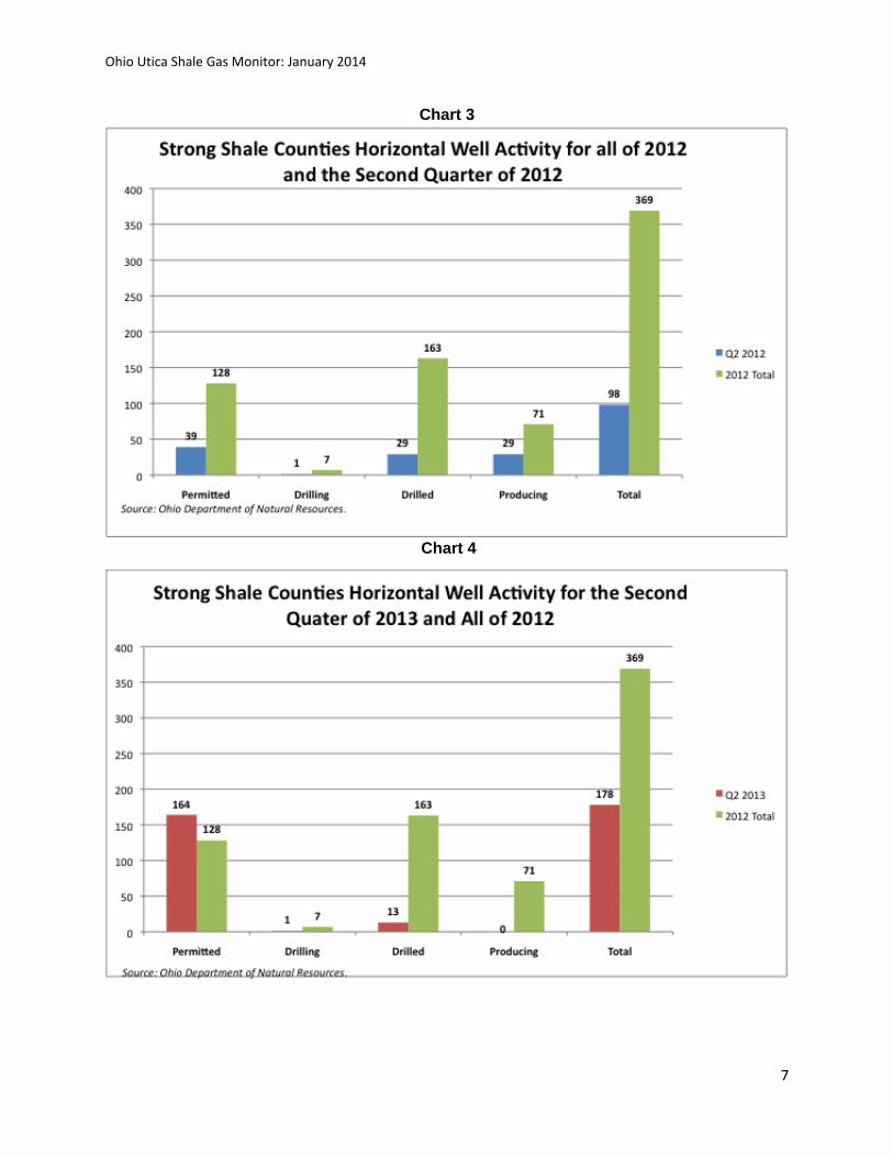
• Permitting of horizontal natural gas wells continued at a rapid pace but midstream

infrastructure challenges remain. An additional 164 wells were permitted during the

second quarter of 2013 alone, an increase of 321% compared to the same quarter of

2012. However, the number of new wells producing oil and gas through the second

quarter of 2013 (2) dropped off compared to the first half of 2012 (46).

• Growth in sales receipts correlates with the rapid increase in the number of wells

permitted, drilled and the increased production in the counties with strong shale activity.

Year-over-year sales tax receipts enjoyed double digit percentage growth in April

through August 2013, reflecting increased wealth creation.

• Employment in counties with strong shale activity remains a challenge, with relatively flat

employment rates through the second quarter of 2013. As these numbers reflect where

a person lives rather than where they work, commuting patterns likely play a role in the


3

data. Hiring is taking place in the metropolitan areas in the moderate shale counties

where field service firms have established operations. In addition, non-shale-related

sectors have absorbed a number of restructurings, potentially impacting the data.

• As of December 18, 2013, Ohio’s Utica formation had 39 active drilling rigs. In

comparison, Ohio’s Marcellus formation had 2 rigs active.

• Larger economic benefits will be reaped if ethane is “cracked” into its commercially

valuable components in or close to Ohio. Potential benefits will be reduced if the NGLs

are either barged or piped to Louisiana or Texas. Interest, intent and investments are

being announced:

o In September 2013, U.K. based Velosys announced its intent to build a plant to

convert natural gas to diesel fuel and other liquids in Ashtabula, Ohio.

o In November 2013, Brazil’s Odebrecht announced Project ASCENT

(Appalachian Shale Cracker Enterprise) to build an ethane cracker and three

polyethylene plants in West Virginia.

o Plastic’s News reported that Canada’s NOVA Chemicals Corp was able to

convert ethane from the Marcellus shale basin to ethylene. As a result, the

company intends to increase the amount of ethane it uses in its Corunna,

Ontario, ethylene plant and to expand the capacity of its Coruna cracker at the

same location by 20 percent by 2018.

o In December 2013, Shell rolled over its option on land near Pittsburgh for the

third time. Shell committed to begin clearing the site in the first quarter of 2014,

however, the company has not publicly announced a decision on building an

ethylene cracker. The length of this option was reported by the Pittsburgh Post-

Gazette to be confidential.

COUNTY CLASSIFICATIONS AND TRENDS

• Drilling and permitting have shifted in recent months, indicating the industry is migrating

activity south and east, focusing its areas of investment. The number of counties with

strong shale activity has gone to eight from 15, and moderate activity has gone to five

from 30.


4

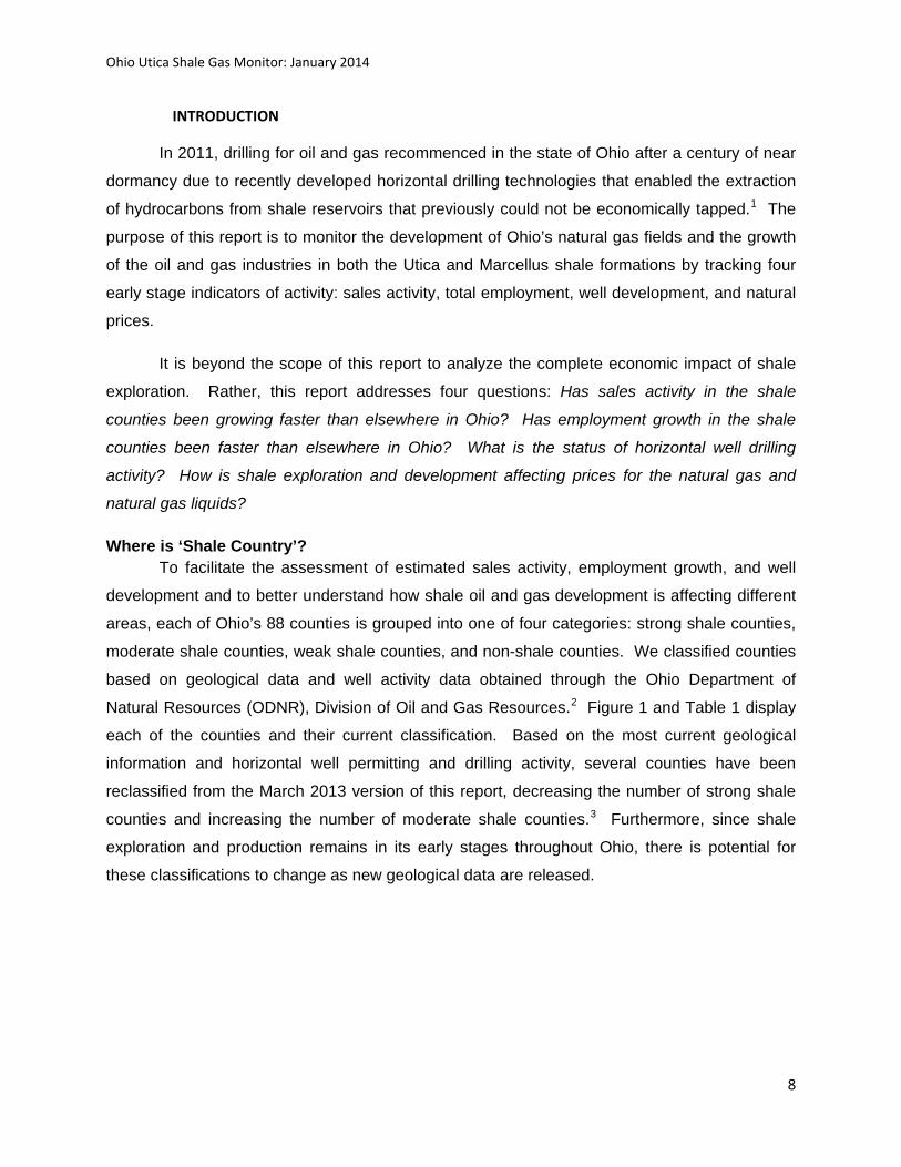
• Strong shale counties have the highest potential for producing commercial amounts of

NGLs. There strong shale counties are along Ohio’s eastern border in the Northern

Appalachian portion of the state: Belmont, Carroll, Columbiana, Guernsey, Harrison,

Jefferson, Monroe, and Noble.

• Moderate shale counties are to the north and immediate west of the strong counties.

Mahoning, Portage, Stark, Trumbull, and Tuscarawas are the five moderate counties.

• Weak shale counties are part of the Utica formation and have deposits of natural gas but

have not proven to hold NGLs. There are 30 such counties that range north to Lake Erie,

west of the city of Columbus, and south to Hocking and Washington counties.

• Forty-five counties are considered to be “non-shale” because of their geology.

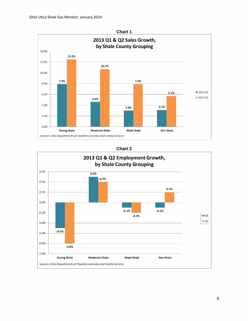
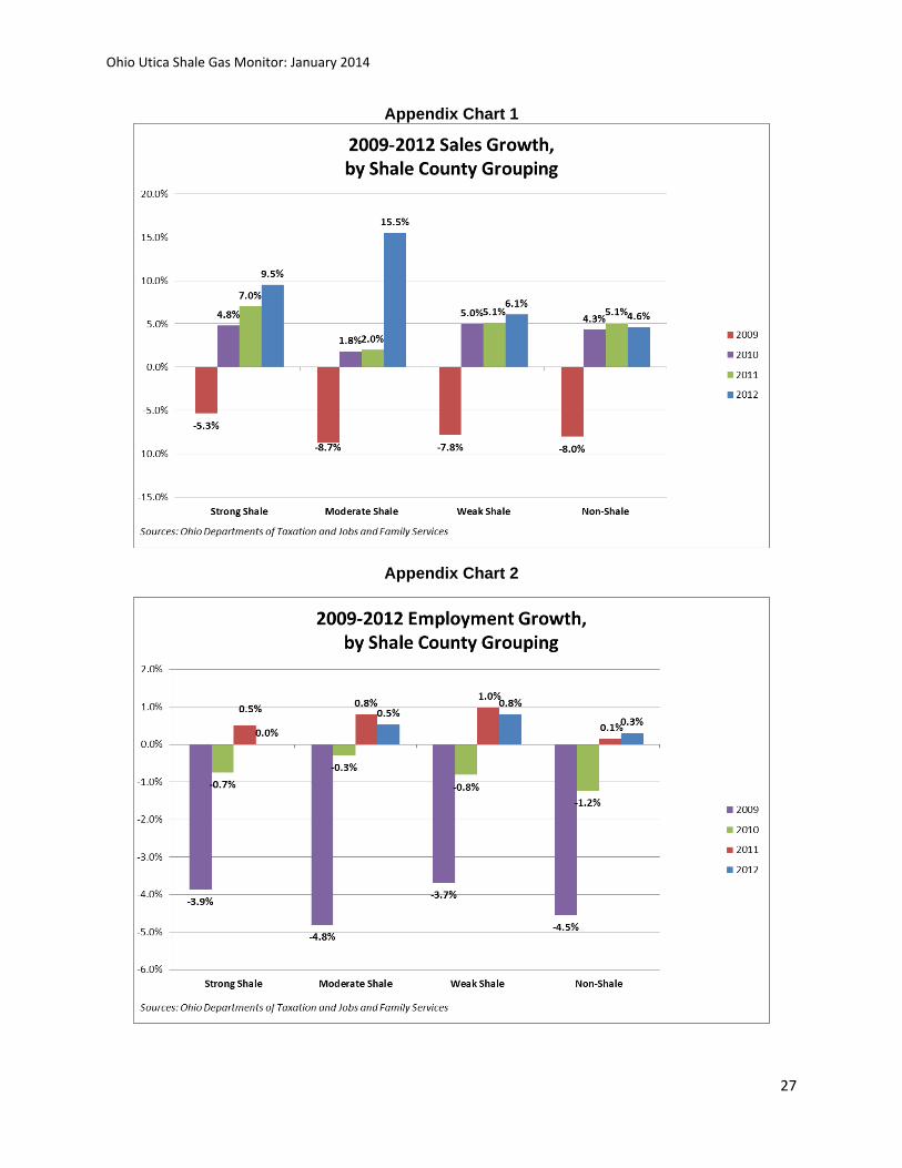
There were marked increases in sales receipts during 2012 and the first two quarters of

2013 in the strong shale counties. Through August 2013, sales receipts in strong shale counties

continued their steady growth. Second-quarter sales receipts increased by 12.2% ($1.3 billion)

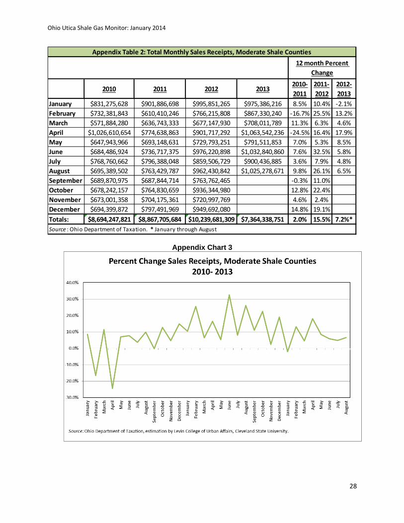
over Q2 2012 ($1.16 billion) (Chart 1). Moderate shale counties also saw solid growth, with

estimated sales increasing by 10.7% in Q2. Sales in both the strong and moderate shale

counties continued to outperform sales in weak shale and non-shale counties, continuing a

trend that goes back to 2009 (Appendix Chart 1).

Increased sales reflect spending by land and mineral rights owners as well as spending

of out-of-state workers because hotel and lodging bills are subject to the sales and use tax in

Ohio, as are restaurant meals. Robust increases in sales in the moderate shale counties reflect

their locations: the Canton and Youngstown-Warren metropolitan areas border the group of

strong shale counties and are located in moderately strong shale counties. Akron and Summit

County have easy access to shale country and benefits from spending, as it is a major retail

destination for northern Appalachian Ohio. These metropolitan areas have larger populations

and stronger retailing presence than do the much more rural strong shale counties.

Employment among the residents of these counties has yet to show substantial gains.

The moderate shale counties performed the best as employment increased by .5% in Q1 and

.4% in Q2. Surprisingly, employment growth was the weakest in the strong shale counties,


5

dipping by -.5% in Q1 and -.8% Q2. Employment in the weak and non-shale counties remained

relatively stable.


6

Chart 1

Chart 2


7

Chart 3

Chart 4


8

INTRODUCTION

In 2011, drilling for oil and gas recommenced in the state of Ohio after a century of near

dormancy due to recently developed horizontal drilling technologies that enabled the extraction

of hydrocarbons from shale reservoirs that previously could not be economically tapped.1 The

purpose of this report is to monitor the development of Ohio’s natural gas fields and the growth

of the oil and gas industries in both the Utica and Marcellus shale formations by tracking four

early stage indicators of activity: sales activity, total employment, well development, and natural

prices.

It is beyond the scope of this report to analyze the complete economic impact of shale

exploration. Rather, this report addresses four questions: Has sales activity in the shale

counties been growing faster than elsewhere in Ohio? Has employment growth in the shale

counties been faster than elsewhere in Ohio? What is the status of horizontal well drilling

activity? How is shale exploration and development affecting prices for the natural gas and

natural gas liquids?

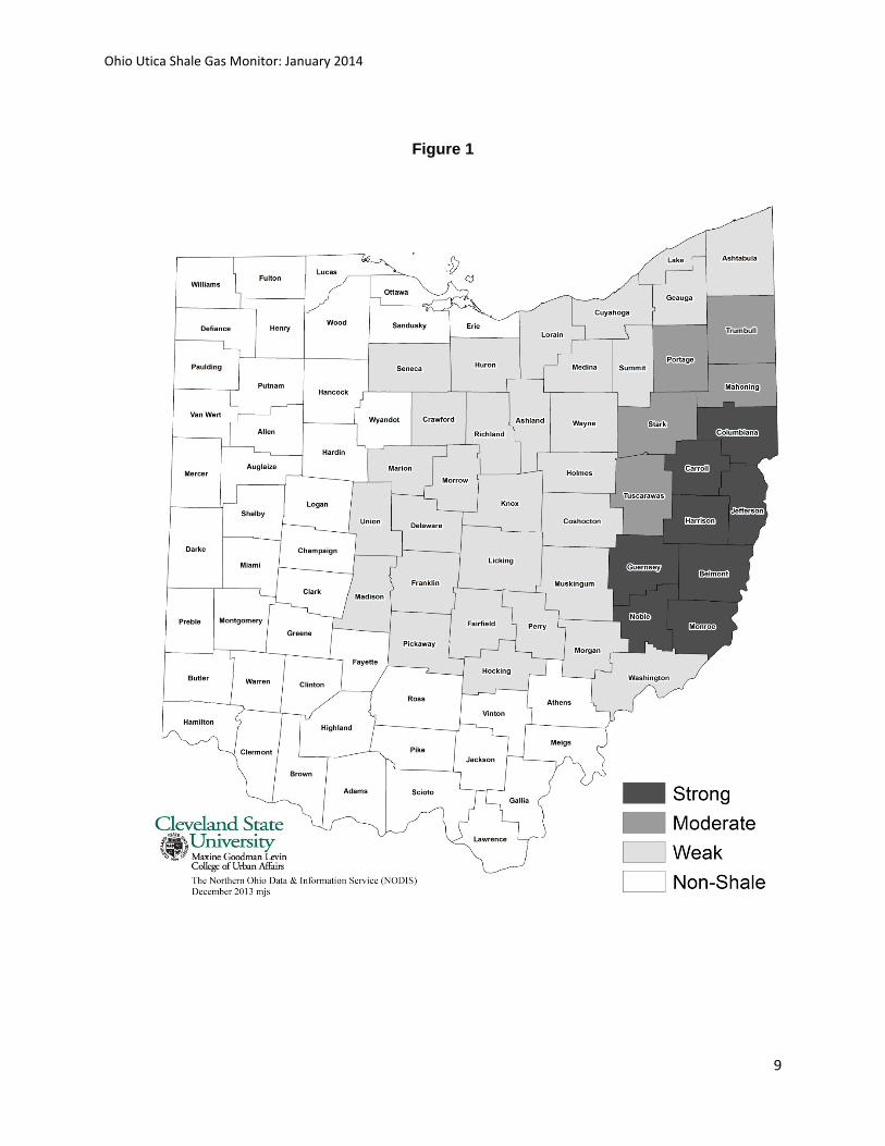
Where is ‘Shale Country’? To facilitate the assessment of estimated sales activity, employment growth, and well

development and to better understand how shale oil and gas development is affecting different

areas, each of Ohio’s 88 counties is grouped into one of four categories: strong shale counties,

moderate shale counties, weak shale counties, and non-shale counties. We classified counties

based on geological data and well activity data obtained through the Ohio Department of

Natural Resources (ODNR), Division of Oil and Gas Resources.2 Figure 1 and Table 1 display

each of the counties and their current classification. Based on the most current geological

information and horizontal well permitting and drilling activity, several counties have been

reclassified from the March 2013 version of this report, decreasing the number of strong shale

counties and increasing the number of moderate shale counties.3 Furthermore, since shale

exploration and production remains in its early stages throughout Ohio, there is potential for

these classifications to change as new geological data are released.


9

Figure 1


10

Strong (n=8) Moderate (n= 5) Weak (n=30)Non-shale

(n= 45)Belmont Mahoning Ashland AdamsCarroll Portage Ashtabula Allen

Columbiana Stark Coshocton AthensGuernsey Trumbull Crawford AuglaizeHarrison Tuscarawas Cuyahoga BrownJefferson Delaware ButlerMonroe Fairfield ChampaignNoble Franklin Clark

Geauga ClermontHocking ClintonHolmes DarkeHuron DefianceKnox ErieLake Fayette

Licking FultonLorain Gallia

Madison GreeneMarion HamiltonMedina HancockMorgan HardinMorrow Henry

Muskingum HighlandPerry Jackson

Pickaway Lawrence Richland LoganSeneca Lucas

Summitt MeigsUnion Mercer

Washington MiamiWayne Montgomery

OttawaPaulding

Pike Preble

PutnamRoss

SanduskyScioto Shelby

Van WertVintonWarren

WilliamsWood

Wyandot

Table 1: County Classifications (n=88)


11

RESULTS

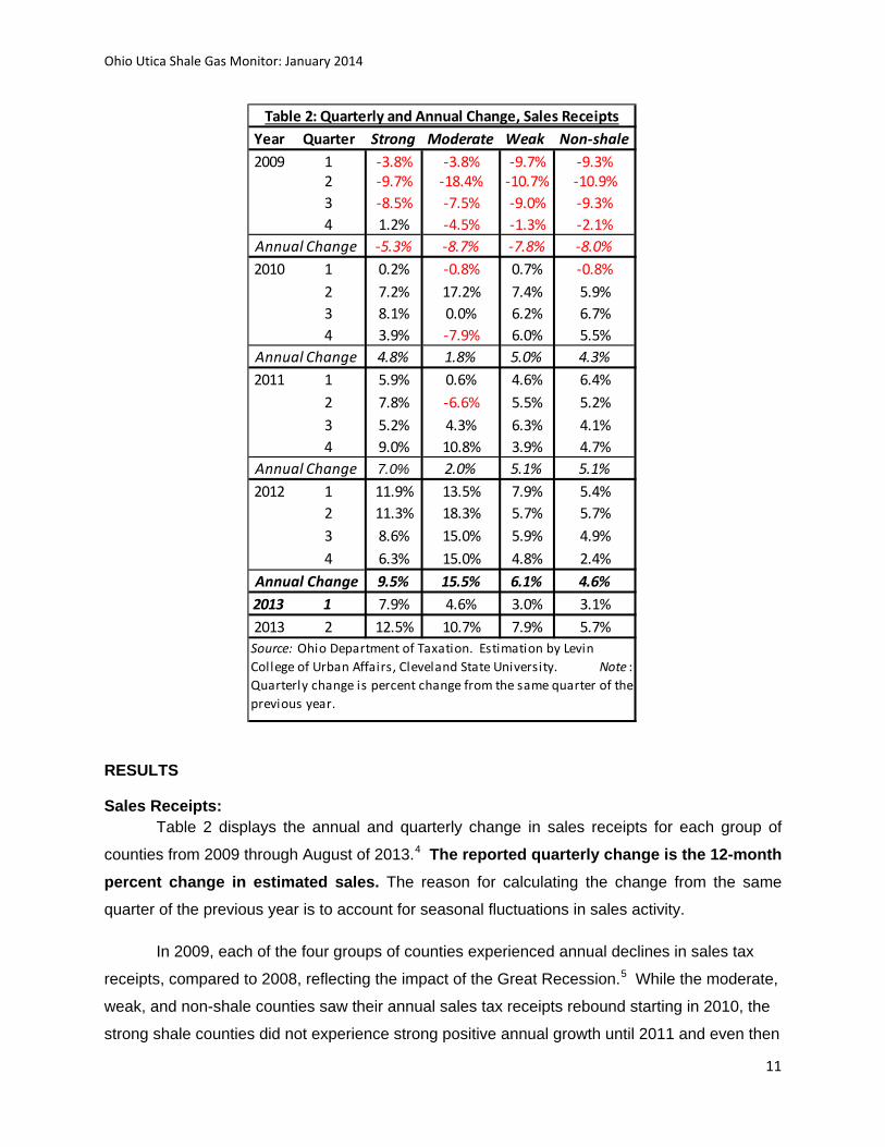
Sales Receipts: Table 2 displays the annual and quarterly change in sales receipts for each group of

counties from 2009 through August of 2013.4 The reported quarterly change is the 12-month percent change in estimated sales. The reason for calculating the change from the same

quarter of the previous year is to account for seasonal fluctuations in sales activity.

In 2009, each of the four groups of counties experienced annual declines in sales tax

receipts, compared to 2008, reflecting the impact of the Great Recession.5 While the moderate,

weak, and non-shale counties saw their annual sales tax receipts rebound starting in 2010, the

strong shale counties did not experience strong positive annual growth until 2011 and even then

Year Quarter Strong Moderate Weak Non-shale2009 1 -3.8% -3.8% -9.7% -9.3%

2 -9.7% -18.4% -10.7% -10.9%3 -8.5% -7.5% -9.0% -9.3%4 1.2% -4.5% -1.3% -2.1%

-5.3% -8.7% -7.8% -8.0%2010 1 0.2% -0.8% 0.7% -0.8%

2 7.2% 17.2% 7.4% 5.9%3 8.1% 0.0% 6.2% 6.7%4 3.9% -7.9% 6.0% 5.5%

4.8% 1.8% 5.0% 4.3%2011 1 5.9% 0.6% 4.6% 6.4%

2 7.8% -6.6% 5.5% 5.2%3 5.2% 4.3% 6.3% 4.1%4 9.0% 10.8% 3.9% 4.7%

7.0% 2.0% 5.1% 5.1%2012 1 11.9% 13.5% 7.9% 5.4%

2 11.3% 18.3% 5.7% 5.7%3 8.6% 15.0% 5.9% 4.9%4 6.3% 15.0% 4.8% 2.4%

9.5% 15.5% 6.1% 4.6%2013 1 7.9% 4.6% 3.0% 3.1%2013 2 12.5% 10.7% 7.9% 5.7%

Source: Ohio Department of Taxation. Estimation by Levin College of Urban Affairs, Cleveland State University. Note : Quarterly change is percent change from the same quarter of the previous year.

Annual Change

Annual Change

Annual Change

Annual Change

Table 2: Quarterly and Annual Change, Sales Receipts


12

the change was very small. By the first quarter of 2012, however, this relationship among the

counties turned around. The strong and moderate shale counties experienced double-digit

growth in sales receipts, reaching a peak of 18.3% growth rate in the third quarter in moderate

shale counties, and growing at an annual rate of 15.5%. Sales receipts increased 9.5% over

2012. This growth far outpaced the growth in sales receipts in the weak and non-shale counties

during 2012.6 Rapid growth in sales receipts in strong and moderate shale counties has

continued through the second quarter of 2013 and remains faster than sales growth elsewhere

in the state.

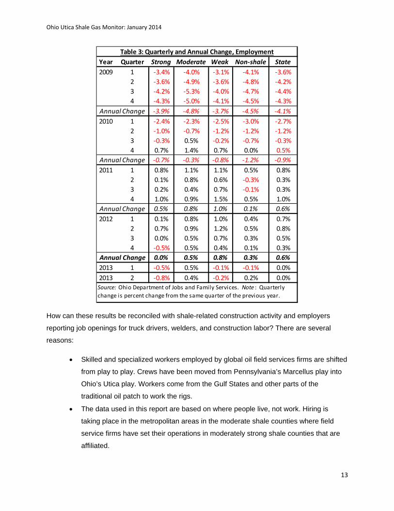
Total Employment: Table 3 reflects the annual and quarterly changes in total employment for each group of

counties between 2009 and the third quarter of 2013. The reported quarterly change is the 12-month percent change from the same quarter of the previous year based on a person’s place of residence, not place of work.

The employment trends in 2009 mirrored the declines in sales receipts noted above.

However, unlike rapid growth in sales receipts that were observed in subsequent years, growth

in employment was small in 2011 across all four groups of Ohio’s counties, but the non-shale

counties experienced the least growth.

Employment gains in 2012 were again modest, with the strong shale counties not

experiencing any employment growth. During 2012, state employment increased 0.6% and the

weak shale counties experienced the most growth at 0.8%.

Through the second quarter of 2013, employment growth among the residents of shale

country has again stagnated and even declined a bit. Employment among residents in the

strong shale counties has decreased by 0.8% or by about 4,300 persons employed.

Employment in moderate counties has increased slightly, by 0.5% in Q1 and 0.4% in Q2.

Employment in weak counties decreased slightly in 2013, and in non-shale counties it has

increased.


13

How can these results be reconciled with shale-related construction activity and employers

reporting job openings for truck drivers, welders, and construction labor? There are several

reasons:

• Skilled and specialized workers employed by global oil field services firms are shifted

from play to play. Crews have been moved from Pennsylvania’s Marcellus play into

Ohio’s Utica play. Workers come from the Gulf States and other parts of the

traditional oil patch to work the rigs.

• The data used in this report are based on where people live, not work. Hiring is

taking place in the metropolitan areas in the moderate shale counties where field

service firms have set their operations in moderately strong shale counties that are

affiliated.

Year Quarter Strong Moderate Weak Non-shale State2009 1 -3.4% -4.0% -3.1% -4.1% -3.6%

2 -3.6% -4.9% -3.6% -4.8% -4.2%3 -4.2% -5.3% -4.0% -4.7% -4.4%4 -4.3% -5.0% -4.1% -4.5% -4.3%

-3.9% -4.8% -3.7% -4.5% -4.1%2010 1 -2.4% -2.3% -2.5% -3.0% -2.7%

2 -1.0% -0.7% -1.2% -1.2% -1.2%3 -0.3% 0.5% -0.2% -0.7% -0.3%4 0.7% 1.4% 0.7% 0.0% 0.5%

-0.7% -0.3% -0.8% -1.2% -0.9%2011 1 0.8% 1.1% 1.1% 0.5% 0.8%

2 0.1% 0.8% 0.6% -0.3% 0.3%3 0.2% 0.4% 0.7% -0.1% 0.3%4 1.0% 0.9% 1.5% 0.5% 1.0%

0.5% 0.8% 1.0% 0.1% 0.6%2012 1 0.1% 0.8% 1.0% 0.4% 0.7%

2 0.7% 0.9% 1.2% 0.5% 0.8%3 0.0% 0.5% 0.7% 0.3% 0.5%4 -0.5% 0.5% 0.4% 0.1% 0.3%

0.0% 0.5% 0.8% 0.3% 0.6%2013 1 -0.5% 0.5% -0.1% -0.1% 0.0%2013 2 -0.8% 0.4% -0.2% 0.2% 0.0%

Source: Ohio Department of Jobs and Family Services. Note : Quarterly change is percent change from the same quarter of the previous year.

Table 3: Quarterly and Annual Change, Employment

Annual Change

Annual Change

Annual Change

Annual Change


14

• Growth in shale jobs is being offset by employment losses in other industries. For

example, the closure of Ormet’s aluminum smelter complex in the strong shale

Monroe County will ultimately result in the loss of 1,200 jobs. When the closing was

announced in February of 2013 the complex employed nearly 1,200 and at the time

of its closing in October 2013 700 were still at the plant. The state of Ohio estimates

that about half of the workers at Ormet live in Ohio; the remainder are residents of

West Virginia. Another example is employment in coal mining. Statewide the number

of coal mining jobs decreased by 265 from the first quarter of 2012 to the first quarter

of 2013. Much of Ohio’s coal mines are located in the strong shale counties.

Monthly Sales Growth in Strong Shale Counties:

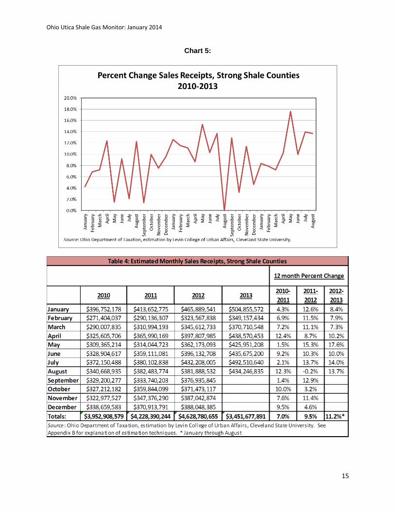
Chart 1 and Table 4 display the 12-month percent change in estimated sales receipts

between 2010 and 2013 for the strong shale counties.7 The positive trend in sales receipts

begins in May 2011 and continues through the first quarter of 2013. This turnaround and

subsequent growth in sales receipts correlates with the rapid increase in the number of wells

permitted, drilled, and the increase in production in strong shale counties (see Table 5). These

counties experienced a 20.4% increase in total sales activity in 2012 ($15.5 billion), compared

to 2011 ($12.8 billion). Sales receipt growth was robust in strong shale counties through the

first quarter of 2013, with growth at or above 10% during each of the first three months. This

continues to be the fastest growth in the state.


15

Chart 5:


16

Well Activity:

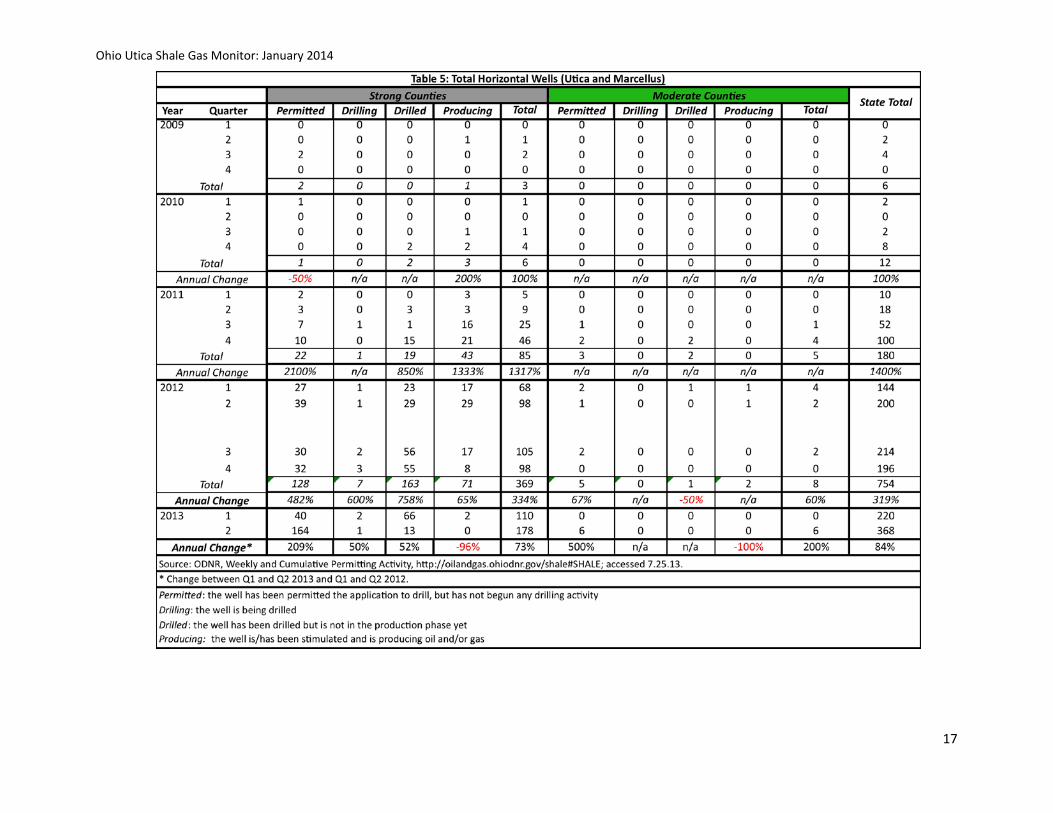
Table 5 summarizes horizontal well activity in strong and moderate counties between

2009 and the second quarter of 2013. Activity is divided into four categories:8

• Permitted: the well has been permitted but drilling activity has not begun

• Drilling: the well is being drilled

• Drilled: the well has been drilled but is not in the production phase

• Producing: the well is/has been stimulated and is producing gas, natural gas liquids,

and/or oil

Permitting and producing activity began to take off during the third quarter of 2011 and

all types of well activity grew steadily through 2012 in the strong shale counties. By the end of

2012, the number of horizontal wells drilled in the strong shale counties had increased by 758%

from the previous year, while the number of wells permitted had climbed by 482%. During

2013, well permitting continued at a rampant pace, with an additional 164 wells permitted during

the second quarter of 2013 alone, an increase of 321% compared to the same quarter of 2012.

However, the number of new wells producing oil and gas through the second quarter of 2013 (2)

has dropped off compared to the first half of 2012 (46). This reflects the fact that the midstream

infrastructure was not yet fully built out.


17


18

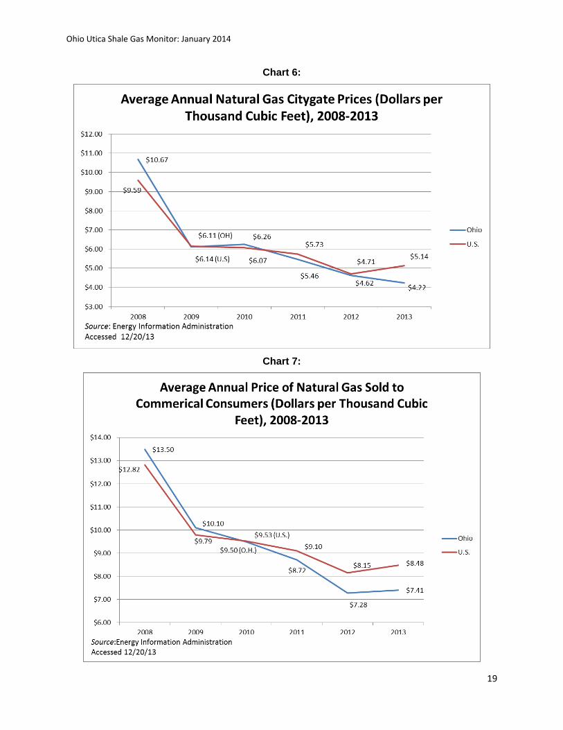
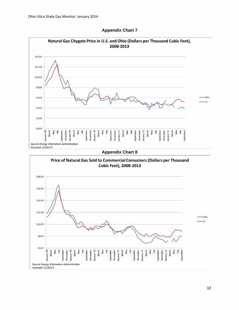
Natural Gas Prices and Production:

Changes in the monthly Citygate price of natural gas and the price paid by commercial

consumers are charted from 2008 through August 2013 using data from the Energy Information

Administration (EIA).9 Natural gas price trends in Ohio mirror those at the national level, as

depicted in Charts 4 and 5. Starting in 2011, both the Citygate and commercial gas prices in

Ohio began to dip below the average national prices, although this trend is a bit stronger in

commercial gas prices.10

In both Ohio and the U.S., the average Citygate price of natural gas (-58%, OH; -49%,

U.S) and the average price for commercial consumers (-47%, OH; -37%, U.S.) fell precipitously

between 2008 and 2011 reflecting the surge in supply of this product. Since shale production

took off in Ohio during the third quarter of 2011, average prices for natural gas have remained

below the national average. Between 2011 and 2012 the average Citygate price in Ohio fell

from $5.46 to $4.62. In 2013, this pricing trend accelerated and the gap in prices widened;

Ohio’s Citygate prices were 85 cents lower than the national average and $1.12 lower for

commercial consumers.

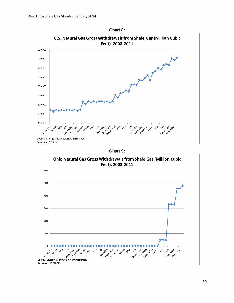
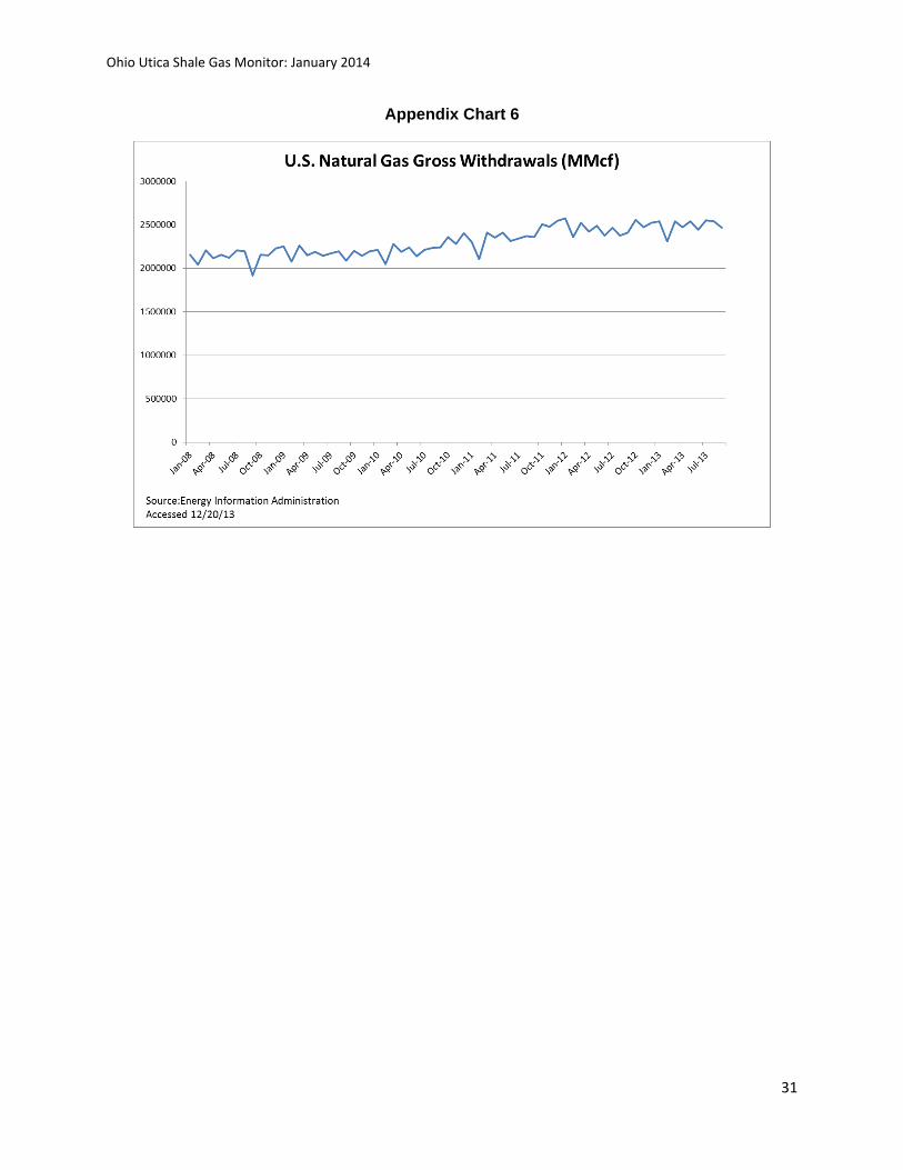
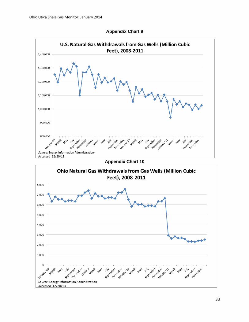
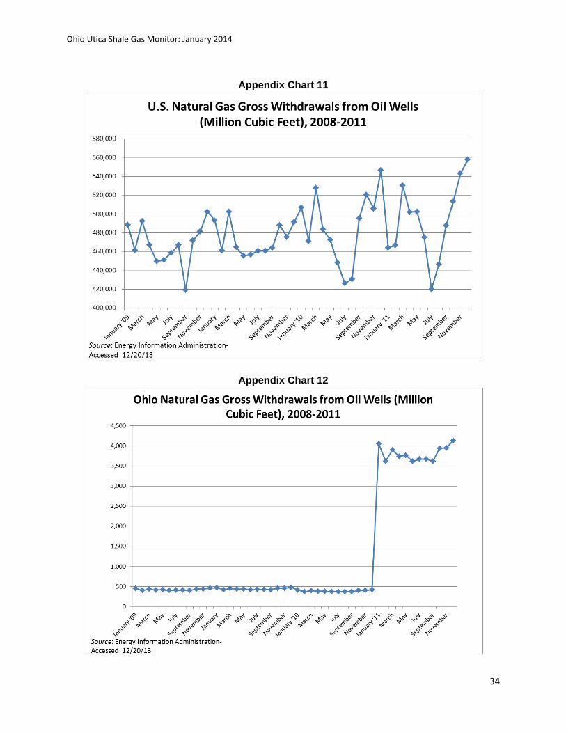
The EIA’s data on gross natural gas withdrawals of shale gas between 2008 and 2011 is

graphed for Ohio and United States.11 Chart 6 shows the overall increase in shale gas

production across the U.S., with gross withdrawals increasing from an average of approximately

240,000 million cubic feet in 2008 to over 700,000 million cubic feet in 2011 (an increase of

196%). By contrast, Ohio’s growth in shale gas production did not begin until 2011 and takes

off in the third quarter of that year (see Chart 7 and Table 5) with gross gas withdrawals from

shale gas reaching 480 million cubic feet in December 2011.12

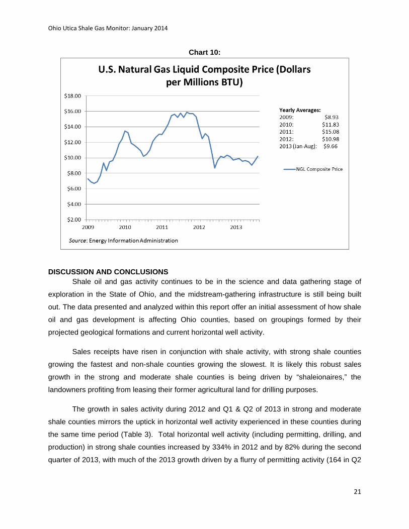
Finally, Chart 8 displays the U.S. Natural Gas Liquid Composite Price (Dollars per Million

BTUs) between 2009 and August 2013.13 Average prices peaked in 2011 at just over $15 per

million BTUs, fell by 27% in 2012 ($10.98) and by another 13% through August 2013 ($9.66).


19

Chart 6:

Chart 7:


20

Chart 8:

Chart 9:


21

Chart 10:

DISCUSSION AND CONCLUSIONS Shale oil and gas activity continues to be in the science and data gathering stage of

exploration in the State of Ohio, and the midstream-gathering infrastructure is still being built

out. The data presented and analyzed within this report offer an initial assessment of how shale

oil and gas development is affecting Ohio counties, based on groupings formed by their

projected geological formations and current horizontal well activity.

Sales receipts have risen in conjunction with shale activity, with strong shale counties

growing the fastest and non-shale counties growing the slowest. It is likely this robust sales

growth in the strong and moderate shale counties is being driven by “shaleionaires,” the

landowners profiting from leasing their former agricultural land for drilling purposes.

The growth in sales activity during 2012 and Q1 & Q2 of 2013 in strong and moderate

shale counties mirrors the uptick in horizontal well activity experienced in these counties during

the same time period (Table 3). Total horizontal well activity (including permitting, drilling, and

production) in strong shale counties increased by 334% in 2012 and by 82% during the second

quarter of 2013, with much of the 2013 growth driven by a flurry of permitting activity (164 in Q2


22

2013 alone). While this analysis cannot specify the direct impact of shale development on sales

activity, there is a relationship between the two variables.

Total employment growth has been much less robust than sales activity in Ohio’s shale

country. However, strong (0.1%) and moderate (0.2%) shale counties did experience very

modest growth in total employment growth during the second quarter of 2013, while all other

county groups experienced small declines in total employment- weak (-0.1%) and non-shale

(-1.6%). This muted employment growth can be attributed to several factors. First, as others

within the shale arena have noted, Ohio’s workforce is still being trained and prepared to work

within the oil and gas industry.14 Second, as the midstream development -- “the system of

pipelines and processing plants that will take the hydrocarbons from the well pad to the end-

user, whether it's a chemical company, a refinery or your BBQ grill”-- continues and improves

market access over the next several years, production numbers are predicted to continue rising

and associated job growth will accompany these developments.15 Lastly, the employment data

analyzed here reflects total employment in Ohio counties and does not specifically focus on

sectors or industries (i.e. manufacturing, construction, transportation) that are more likely to be

more directly impacted by shale development.

Critical to the development of the natural gas resources in Ohio is the price of natural

gas liquids (NGLs) and dry gas or methane. With the advent of horizontal drilling and hydraulic

fracking technologies, large volumes of dry natural gas can be extracted from a number of shale

formations throughout the country. Despite the fact that the price of dry gas has increased from

$3 to about $5 per thousand cubic feet (nationally), it is unlikely to rise until the conversion of

the U.S. economy from a predominantly oil and coal powered economy to natural gas power is

further along.

The various shale gas fields, or plays, will be developed based on the value of their

component resources—oil, NGLs, and dry gas. The excitement over the Utica Shale in Ohio is

based on the limited presence of oil in the formation and the much more extensive presence of

NGLs. However, the degree to which the presence of NGLs changes the mid-term economic

landscape of Ohio depends in no small part on where the NGLs are processed. This is

especially so for ethane, a critical building block of industrial plastics. Large benefits will be

reaped if ethane is “cracked” into its commercially valuable components in or close to Ohio.

Potential benefits will be reduced if it is barged or piped to Louisiana or Texas.


23

In September 2013, U.K.-based Velosys announced its intent to build a plant to convert

natural gas to diesel fuel and other liquids in Ashtabula, Ohio. In November 2013, Brazil’s

Odebrecht announced Project ASCENT (Appalachian Shale Cracker Enterprise) to build an

ethane cracker and three polyethylene plants in West Virginia. Plastic’s News reported that

Canada’s NOVA Chemicals Corp was able to convert ethane from the Marcellus shale basin to

ethylene. As a result, the company intends to increase the amount of ethane it uses in its

Corunna, Ontario, ethylene plant and to expand the capacity of its Corruna cracker at the same

location by 20 percent by 2018. Finally, in December 2013, Shell rolled over its option on land

near Pittsburgh for the third time. Shell committed to begin clearing the site in the first quarter of

2014, however, the company has not publicly announced a decision on an ethylene cracker. Its

announcement came weeks after Shell said it was pulling out of a similar investment in

Louisiana. The length of this option was reported by the Pittsburgh Post-Gazette to be

confidential.

Since 2011, Ohio natural gas production has been increasing, but remains a small

fraction of the national supply. As the market for Ohio’s natural gas grows with production, so

will the economic benefits. Through Q2 of 2013, shale’s impact on sales receipts is highly

encouraging if employment is able to catch up.


24

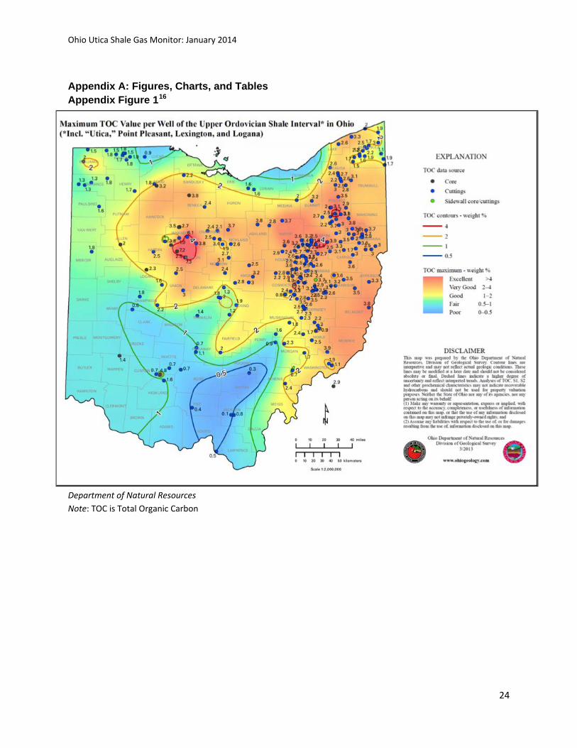
Appendix A: Figures, Charts, and Tables Appendix Figure 116

Source: Ohio

Department of Natural Resources Note: TOC is Total Organic Carbon


25

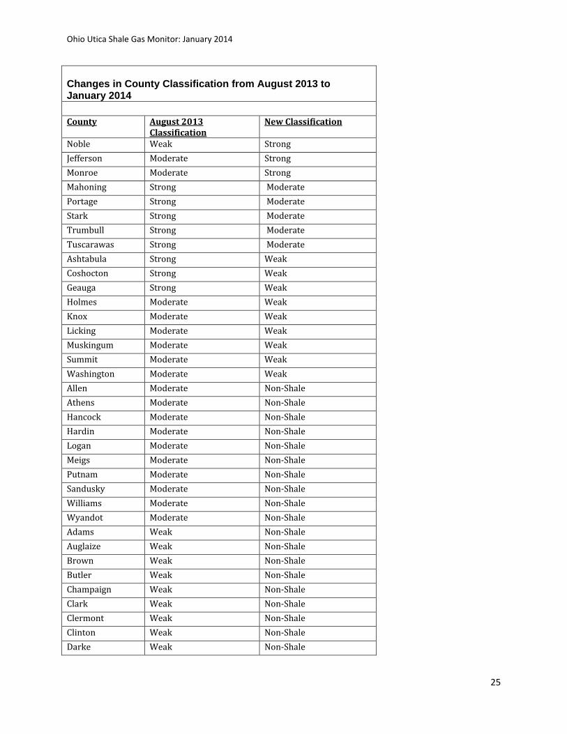
Changes in County Classification from August 2013 to January 2014 County August 2013

Classification New Classification

Noble Weak Strong Jefferson Moderate Strong Monroe Moderate Strong Mahoning Strong Moderate Portage Strong Moderate Stark Strong Moderate Trumbull Strong Moderate Tuscarawas Strong Moderate Ashtabula Strong Weak Coshocton Strong Weak Geauga Strong Weak Holmes Moderate Weak Knox Moderate Weak Licking Moderate Weak Muskingum Moderate Weak Summit Moderate Weak Washington Moderate Weak Allen Moderate Non-Shale Athens Moderate Non-Shale Hancock Moderate Non-Shale Hardin Moderate Non-Shale Logan Moderate Non-Shale Meigs Moderate Non-Shale Putnam Moderate Non-Shale Sandusky Moderate Non-Shale Williams Moderate Non-Shale Wyandot Moderate Non-Shale Adams Weak Non-Shale Auglaize Weak Non-Shale Brown Weak Non-Shale Butler Weak Non-Shale Champaign Weak Non-Shale Clark Weak Non-Shale Clermont Weak Non-Shale Clinton Weak Non-Shale Darke Weak Non-Shale


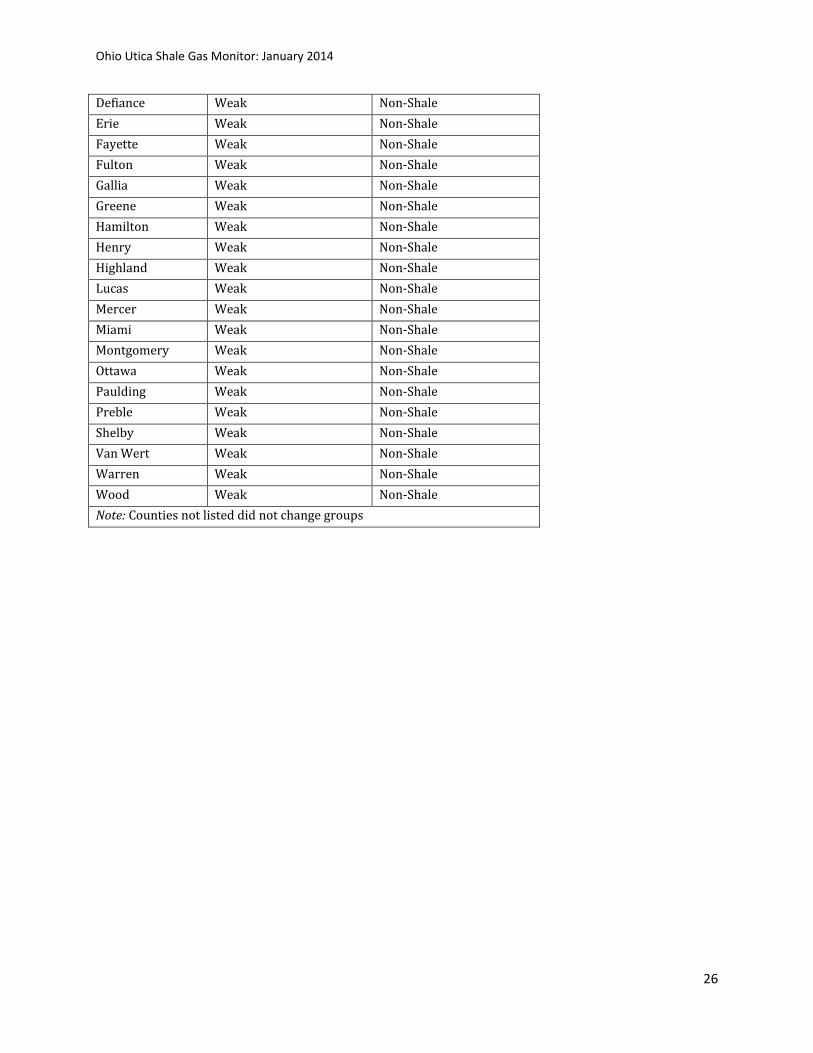
26

Defiance Weak Non-Shale Erie Weak Non-Shale Fayette Weak Non-Shale Fulton Weak Non-Shale Gallia Weak Non-Shale Greene Weak Non-Shale Hamilton Weak Non-Shale Henry Weak Non-Shale Highland Weak Non-Shale Lucas Weak Non-Shale Mercer Weak Non-Shale Miami Weak Non-Shale Montgomery Weak Non-Shale Ottawa Weak Non-Shale Paulding Weak Non-Shale Preble Weak Non-Shale Shelby Weak Non-Shale Van Wert Weak Non-Shale Warren Weak Non-Shale Wood Weak Non-Shale Note: Counties not listed did not change groups


27

Appendix Chart 1

Appendix Chart 2


28

Appendix Chart 3

2010- 2011- 2012-2011 2012 2013

January $831,275,628 $901,886,698 $995,851,265 $975,386,216 8.5% 10.4% -2.1%February $732,381,843 $610,410,246 $766,215,808 $867,330,240 -16.7% 25.5% 13.2%March $571,884,280 $636,743,333 $677,147,930 $708,011,789 11.3% 6.3% 4.6%April $1,026,610,654 $774,638,863 $901,717,292 $1,063,542,236 -24.5% 16.4% 17.9%May $647,943,966 $693,148,631 $729,793,251 $791,511,853 7.0% 5.3% 8.5%June $684,486,924 $736,717,375 $976,220,898 $1,032,840,860 7.6% 32.5% 5.8%July $768,760,662 $796,388,048 $859,506,729 $900,436,885 3.6% 7.9% 4.8%August $695,389,502 $763,429,787 $962,430,842 $1,025,278,671 9.8% 26.1% 6.5%September $689,870,975 $687,844,714 $763,762,465 -0.3% 11.0%October $678,242,157 $764,830,659 $936,344,980 12.8% 22.4%November $673,001,358 $704,175,361 $720,997,769 4.6% 2.4%December $694,399,872 $797,491,969 $949,692,080 14.8% 19.1%Totals: $8,694,247,821 $8,867,705,684 $10,239,681,309 $7,364,338,751 2.0% 15.5% 7.2%*Source : Ohio Department of Taxation. * January through August

Appendix Table 2: Total Monthly Sales Receipts, Moderate Shale Counties 12 month Percent

Change

2011 2012 20132010


29

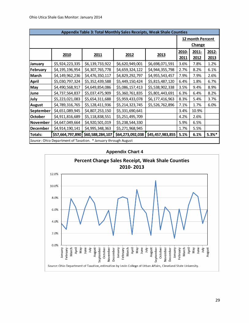
Appendix Chart 4

2010- 2011- 2012-2011 2012 2013

January $5,924,223,335 $6,139,733,922 $6,620,949,001 $6,698,071,591 3.6% 7.8% 1.2%February $4,195,196,954 $4,307,765,778 $4,659,324,122 $4,944,355,798 2.7% 8.2% 6.1%March $4,149,962,236 $4,476,350,117 $4,829,292,797 $4,955,543,457 7.9% 7.9% 2.6%April $5,030,797,324 $5,352,439,588 $5,449,150,424 $5,815,487,120 6.4% 1.8% 6.7%May $4,490,568,917 $4,649,854,086 $5,086,157,413 $5,538,902,338 3.5% 9.4% 8.9%June $4,737,564,837 $5,037,475,909 $5,360,761,835 $5,801,443,691 6.3% 6.4% 8.2%July $5,223,021,083 $5,654,311,688 $5,959,433,078 $6,177,416,963 8.3% 5.4% 3.7%August $4,789,316,765 $5,128,411,936 $5,214,323,745 $5,526,762,896 7.1% 1.7% 6.0%September $4,651,089,945 $4,807,253,150 $5,331,690,641 3.4% 10.9%October $4,911,816,689 $5,118,838,551 $5,251,495,709 4.2% 2.6%November $4,647,049,664 $4,920,501,019 $5,238,544,330 5.9% 6.5%December $4,914,190,141 $4,995,348,363 $5,271,968,945 1.7% 5.5%Totals: $57,664,797,890 $60,588,284,107 $64,273,092,038 $45,457,983,855 5.1% 6.1% 5.3%*Source : Ohio Department of Taxation. * January through August

Appendix Table 3: Total Monthly Sales Receipts, Weak Shale Counties 12 month Percent

Change

2011 2012 20132010


30

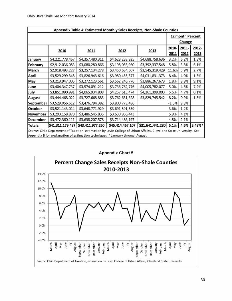
Appendix Chart 5

2010- 2011- 2012-2011 2012 2013

January $4,221,778,467 $4,357,480,311 $4,628,238,925 $4,688,758,636 3.2% 6.2% 1.3%February $2,912,036,083 $3,080,280,866 $3,198,055,960 $3,392,337,548 5.8% 3.8% 6.1%March $2,918,493,227 $3,257,134,278 $3,450,634,507 $3,545,319,429 11.6% 5.9% 2.7%April $3,529,299,348 $3,826,943,616 $3,980,455,377 $4,031,831,373 8.4% 4.0% 1.3%May $3,213,947,005 $3,272,123,561 $3,562,246,776 $3,886,267,673 1.8% 8.9% 9.1%June $3,404,347,737 $3,574,091,212 $3,736,762,776 $4,005,782,077 5.0% 4.6% 7.2%July $3,851,090,991 $4,065,934,808 $4,257,613,474 $4,261,399,003 5.6% 4.7% 0.1%August $3,444,468,022 $3,727,668,885 $3,762,651,628 $3,829,745,542 8.2% 0.9% 1.8%September $3,529,056,612 $3,476,794,382 $3,800,773,486 -1.5% 9.3%October $3,521,143,014 $3,648,771,929 $3,691,591,559 3.6% 1.2%November $3,293,158,870 $3,486,545,835 $3,630,956,443 5.9% 4.1%December $3,472,360,111 $3,638,207,578 $3,714,486,197 4.8% 2.1%Totals: $41,311,179,487 $43,411,977,260 $45,414,467,107 $31,641,441,280 5.1% 4.6% 3.48%*Source : Ohio Department of Taxation, estimation by Levin College of Urban Affairs, Cleveland State University. See Appendix B for explanation of estimation techniques * January through August

Appendix Table 4: Estimated Monthly Sales Receipts, Non-Shale Counties 12 month Percent

Change

2011 2012 20132010


31

Appendix Chart 6


32

Appendix Chart 7

Appendix Chart 8


33

Appendix Chart 9

Appendix Chart 10


34

Appendix Chart 11

Appendix Chart 12


35

Appendix B: Methodology

The following section outlines the methodology used to group Ohio’s counties and to

analyze the sales tax and total employment data throughout this report.

Counties were scored based on total well activity and geological formation:

• Counties with 1-5 wells were given a score of 1

• Counties with 6-24 wells were given a score of 2

• Counties with 25 or more wells were given a score of 3

• Counties with very good to excellent geology were given a score of 4.0-4.5

• Counties with fair/good to very good geology were given a score of 3.0-3.75

• Counties with fair to good geology were given a score of 2.0-2.5

• Counties with poor to good geology were given a score of 0.75

The scores were then added together, and counties were grouped based on natural

breaks within the distribution. Strong counties are those with a score of 5 or greater, moderate

counties between 3 and 5, weak counties between 0.5 and 2.5, and non-shale counties less

than 0.5. Well activity (http://oilandgas.ohiodnr.gov/shale#SHALE) and geological formation

data (http://www.dnr.state.oh.us/Portals/10/Energy/Utica/Ordov-Shale_TOC-Max_03-2013.pdf)

were obtained from the Ohio Department of Natural Resources.

Employment data were sourced from the Ohio Department of Jobs and Family Services,

Civilian Labor Force Estimate.17 The employment data are an estimate of the numbers of

people who live in the county and are employed, not the number of jobs in the county. In other

words, these data are estimated by place of residence instead of place of work.

http://oilandgas.ohiodnr.gov/shale#SHALE

http://www.dnr.state.oh.us/Portals/10/Energy/Utica/Ordov-Shale_TOC-Max_03-2013.pdf


36

Sales tax data were gathered from the Ohio Department of Taxation, Sales Tax

Distributions.18 The estimated sales receipts data were derived from the apportionment

amounts within the Current and Prior Years’ Sales Tax Distribution reports. Sales tax rates are

sourced from the County and Regional Transit Authority Permissive Sales and Use Tax

Collections and Tax Rates, by Month (S1). Both documents are available from the Ohio

Department of Taxation. These reports are inclusive of retail sales activity; business-to-

business transactions are generally exempt under the current Ohio legislative code.

In order to estimate sales receipts from the sales tax data, the sales tax distribution

apportionment amounts were divided by the local sales tax rates.19 This process was

performed for each of Ohio’s 88 counties for each month between January 2008 and October

2013. Although most shale activity did not commence until 2011, data were collected from the

previous three years to allow for comparisons with previous time periods and to be able to

identify trends.

Annual calculations: The annual growth rate was determined by summing the twelve

months of sales receipts/employment for each of the county groupings and calculating the year-

to-year change.

Quarterly calculations: The quarterly growth rate was determined by summing the

three months of sales receipts/employment for each of the county groupings and calculating the

year-to-year change. In other words, the quarterly growth rates for sales receipts and

employment are based on the change from the same quarter in the previous year. For

example, the Q1 2013 growth rate is based on the increase/decrease from Q1 2012.

Monthly calculations: The 12-month percent change for sales receipts and

employment are based on the change from the same month in the previous year.


37

Endnotes 1 Thomas, A.R. et al. (2011). “An Analysis of the Economic Potential for Shale Formations in Ohio.” Ohio Shale Coalition. http://urban.csuohio.edu/publications/center/center_for_economic_development/Ec_Impact_Ohio_Utica_Shale_2012.pdf 2 Ohio Department of Natural Resources, “Shale Well Drilling and Permitting.” Retrieved July 20, 2013, http://oilandgas.ohiodnr.gov/shale#SHALE; Ohio Department of Natural Resources, “Maximum TOC Value per Well of the Upper Ordovician Shale Interval in Ohio.” Retrieved July 20, 2013, http://www.dnr.state.oh.us/Portals/10/Energy/Utica/Ordov-Shale_TOC-Max_03-2013.pdf. 3 Please refer to Appendix Table 1 for a list of reclassified counties and Appendix B for more information on how counties were reclassified. 4 Refer to Appendix B for an explanation of how estimated sales receipts were calculated. 5 The National Bureau of Economic Research, “US Business Cycle Expansions and Contractions,” http://www.nber.org/cycles.html. 6 The exception to this is non-shale counties during the third quarter of 2012. A closer examination of the data revealed this growth was driven by a drastic increase of sales receipts (242%) in Pike County during July 2012. According to the Ohio Department of Taxation, this increase was due to taxpayers taking advantage of the Use Tax Amnesty Program, which was in effect between October 1, 2011 and May 1, 2013, and allowed taxpayers to satisfy their past consumer’s use tax liability without additional penalty (J. Heckert, personal communication, August 1, 2013). 7 Similar charts and tables for the other county groups can be found in Appendix A. Refer to Appendix B for an explanation of how estimated sales receipts were calculated. 8 These categories reflect designations made by ODNR in their weekly and cumulative data of shale permitting activity, http://oilandgas.ohiodnr.gov/shale#SHALE. 9 Energy Information Administration, “Natural Gas Summary,” Retrieved August 9, 2013, http://www.eia.gov/dnav/ng/ng_sum_lsum_dcu_soh_m.htm. The Citygate price refers to “[A] point or measuring station at which a distributing gas utility receives gas from a natural gas pipeline company or transmission system” (http://www.eia.gov/dnav/ng/tbldefs/ng_pri_sum_tbldef2.asp). The commercial price refers to “[T]he price of gas used by nonmanufacturing establishments or agencies primarily engaged in the sale of goods or services such as hotels, restaurants, wholesale and retail stores and other service enterprises; and gas used by local, State and Federal agencies engaged in nonmanufacturing activities” (http://www.eia.gov/dnav/ng/tbldefs/ng_pri_sum_tbldef2.asp). 10 For charts displaying the monthly changes in natural gas prices for both residential and commercial consumers, please refer to Appendix A. 11 EIA data on shale gas production in 2012 was not yet available at the time of this report’s publication. 12 For charts displaying Ohio and U.S. gross withdrawals from gas and oils well, see Appendix A. 13 Natural gas liquids (NGLs) include hydrocarbons such as ethane, propane, butane, isobutene, and pentane. According to the EIA, “[T]he natural gas liquids (NGL) composite price is derived from daily Bloomberg spot price data for natural gas liquids at Mont Belvieu, Texas, weighted by gas processing plant production volumes of each product as reported on Form EIA-816, "Monthly Natural Gas Liquids Report" (EIA, Definitions, Sources and Explanatory Notes http://www.eia.gov/dnav/ng/TblDefs/ng_pri_fut_tbldef2.asp). The prices reported are spot prices, or

http://urban.csuohio.edu/publications/center/center_for_economic_development/Ec_Impact_Ohio_Utica_Shale_2012.pdf

http://urban.csuohio.edu/publications/center/center_for_economic_development/Ec_Impact_Ohio_Utica_Shale_2012.pdf



http://www.nber.org/cycles.html


http://www.eia.gov/dnav/ng/ng_sum_lsum_dcu_soh_m.htm

http://www.eia.gov/dnav/ng/tbldefs/ng_pri_sum_tbldef2.asp

http://www.eia.gov/dnav/ng/tbldefs/ng_pri_sum_tbldef2.asp

http://www.eia.gov/dnav/ng/TblDefs/ng_pri_fut_tbldef2.asp


38

“[T]he price for a one-time open market transaction for immediate delivery of a specific quantity of product at a specific location where the commodity is purchased "on the spot" at current market rates” (EIA, Definitions, Sources and Explanatory Notes http://www.eia.gov/dnav/ng/TblDefs/ng_pri_fut_tbldef2.asp). Natural gas liquids (NGLs) include hydrocarbons such as ethane, propane, butane, isobutene, and pentane. 14 Lendel, I. (2013, May 24). “Look for long-term successes from the Utica shale,” http://www.crainscleveland.com/article/20130524/BLOGS05/130529882/1241/newsletter04 15 Samuel, J. (2013, August 2). “What happened to the shale boom?” http://www.crainscleveland.com/article/20130802/BLOGS05/130739971; Samuel, J. (2013, June 7). “Don't let those early Utica shale production numbers fool you,” http://www.crainscleveland.com/article/20130607/BLOGS05/130609880/-1/blogs05 16 Ohio Department of Natural Resources, “Maximum TOC Value per Well of the Upper Ordovician Shale Interval in Ohio.” Retrieved July 20, 2013, http://www.dnr.state.oh.us/Portals/10/Energy/Utica/Ordov-Shale_TOC-Max_03-2013.pdf. 17 Ohio Department of Jobs and Family Services, “Civilian Labor Force Estimates,” http://ohiolmi.com/asp/laus/vbLaus.htm. 18 Ohio Department of Taxation, “Distributions-Sales Tax,” http://www.tax.ohio.gov/government/distributions_sales_.aspx. 19 The sales tax amounts from the Department of Taxation have two months associated with them: the month allocated, which reflects the month the tax was collected, and the month paid, which reflects the month the revenue is distributed to the counties. The Department’s website explains that "[B]ecause of the time required to process tax returns and to identify the proper permissive tax amounts for each county and transit authority, the revenue from the monthly collections is distributed to the counties and regional transit authorities in the second month following the collection month. For example, this means that sales made in January are primarily reflected in February collections, which are distributed as revenue to the counties and transit authorities in April.” The months/years displayed in the tables throughout this report reflect the month allocated, or when the tax was collected. Note that this is a change from how the data were reported in the March 2013 version of this report. Additionally, the local sales tax in Stark County expired in July 2011 and was reinstated in April 2012. In order to maintain an unskewed dataset, sales data for Stark County data from October 2011 to June 2012 were estimated using the average growth rate of the five previous months (5.4%).

http://www.eia.gov/dnav/ng/TblDefs/ng_pri_fut_tbldef2.asp

http://www.crainscleveland.com/article/20130524/BLOGS05/130529882/1241/newsletter04

http://www.crainscleveland.com/article/20130802/BLOGS05/130739971

http://www.crainscleveland.com/article/20130607/BLOGS05/130609880/-1/blogs05



http://ohiolmi.com/asp/laus/vbLaus.htm

http://www.tax.ohio.gov/government/distributions_sales_.aspx

Documents

Ohio Utica Shale Gas Monitor - Blue Racer Midstream Utica Shale Gas Monitor: January 2014 2 EXECUTIVE SUMMARY This report analyzes aggregate indicators of economic activity related