Embed Size (px)
Citation preview
atmosphere
Article
Gathering Pipeline Methane Emissions in Utica ShaleUsing an Unmanned Aerial Vehicle andGround-Based Mobile Sampling
Hugh Z. Li 1,* , Mumbi Mundia-Howe 2, Matthew D. Reeder 2 and Natalie J. Pekney 3
1 Oak Ridge Institute for Science and Education, National Energy Technology Laboratory,Pittsburgh, PA 15236, USA
2 Leidos, National Energy Technology Laboratory, Pittsburgh, PA 15236, USA;[email protected] (M.M.-H.); [email protected] (M.D.R.)
3 U.S. Department of Energy, National Energy Technology Laboratory, Pittsburgh, PA 15236, USA;[email protected]
* Correspondence: [email protected]; Tel.: +1-412-386-6530
Received: 20 May 2020; Accepted: 1 July 2020; Published: 5 July 2020�����������������
Abstract: The United States Environmental Protection Agency Greenhouse Gas Inventory onlyrecently updated the emission factors of natural gas gathering pipelines in April 2019 from theprevious estimates based on a 1990s study of distribution pipelines. Additional measurements areneeded from different basins for more accurate assessments of methane emissions from natural gasmidstream industries and hence the overall climate implications of natural gas as the interim majorenergy source for the next decade. We conducted an unmanned aerial vehicle (UAV) survey and aground-based vehicle sampling campaign targeting gathering pipeline systems in the Utica Shalefrom March to April in 2019. Out of 73 km of pipeline systems surveyed, we found no leaks onpipelines and two leaks on an accessory block valve with leak rates of 3.8 ± 0.4 and 7.6 ± 0.8 mg/s.The low leak frequency phenomenon was also observed in the only existing gathering pipeline studyin Fayetteville Shale. The UAV sampling system facilitated ease of access, broadened the availabilityof pipelines for leak detection, and was estimated to detect methane leaks down to 0.07 g/s usingGaussian dispersion modeling. For future UAV surveys adopting similar instrument setup anddispersion models, we recommend arranging controlled release experiments first to understand thesystem’s detection limit and choosing sampling days with steady and low wind speeds (2 m/s).
Keywords: natural gas; methane emissions; UAV; mobile sampling; Gaussian dispersion
1. Introduction
Methane is the main component (76 to 92%, vol%) of natural gas and the second most abundantgreenhouse gas after carbon dioxide (CO2) [1,2]. The combustion of natural gas produces less than halfthe CO2 emitted from coal combustion, and the other combustion byproducts are mainly water [3].With the recent technological advancement of horizontal drilling and hydraulic fracturing, the UnitedStates is experiencing a shale gas boom, with its annual dry natural gas production increased by67 percent from 18 to 30 trillion cubic feet between 2005 and 2018 [4]. In 2017, the United States becamea net natural gas exporter and natural gas is predicted to be the interim major energy source for thenext decade [5,6]. Methane has a short atmospheric lifetime of 10 years compared to hundreds of yearsfor CO2 [7]. However, methane itself has a global warming potential 28-36 times more than that ofCO2 in a time horizon of 100 years [1]. According to Alvarez et al. [8], if the leak rates of methane inthe natural gas supply chain were less than 3.2% of the total natural gas production, the utilization ofnatural gas would be a short-term mitigation approach for battling climate change and fulfilling the
Atmosphere 2020, 11, 716; doi:10.3390/atmos11070716 www.mdpi.com/journal/atmosphere
Atmosphere 2020, 11, 716 2 of 13
Paris Agreement [9]. Thus, it is essential to accurately characterize methane emissions from differentsegments of the natural gas supply chain [10].
Natural gas gathering operations transport raw gas from production sites to processing plants orinterstate transmission pipelines. Alverez et al. [10] suggested that the gathering system was responsiblefor around 1/5 of methane emissions from the whole natural gas supply chain. In the current UnitedStates Environment Protection Agency (EPA) greenhouse gas inventory (GHGI), emissions factors forgathering pipelines were only recently updated in April 2019 from previous estimates based on a 1996EPA study of distribution pipelines [11]. New measurements of gathering pipelines from differentbasins would help improve inventory estimates.
Few studies directly characterize methane leaks from gathering pipelines [12]. To our knowledge,the only existing study, Zimmerle et al. [12], surveyed 96 km of gathering pipelines in Fayetteville Shalebased on a ground-based mobile sampling platform and concluded that using emission factors frommore recent studies of distribution pipelines would significantly underestimate gathering pipelineemissions. In the study, one underground pipeline leak contributed more than 80% of the total measuredmethane emissions from the gathering pipeline systems in Fayetteville Shale [12]. Aside from thepolicy implication of an accurate methane emission inventory, finding leaks from gathering pipelineshelps avoid a loss of gas, monetary damages, and personal casualty loss [13].
Gathering pipeline systems are mainly composed of three parts: the pipeline, pig launcher,and block valve. Gatherings pipelines are the pipeline segments (1) between oil/gas wells to gatheringcompressor stations and processing plants and (2) connecting these facilities to transmission ordistribution pipelines. The materials of pipelines can be plastic, stainless steel, bare steel, wroughtiron, and cast iron. The cast and wrought iron pipelines were installed over 60 years ago and werelater found to be vulnerable to corrosion. Pipelines more recently built are mostly plastic or stainlesssteel [13]. Gathering pipelines operate at pressures lower than transmission pipelines, typically at arange from 30 to 7720 kPa [14]. Since gathering pipelines are mainly transporting raw gas instead ofthe refined gas, pipeline operators perform pigging exercises to remove debris and deposits in thepipelines and clean the transported gas. Block valves are used for stopping or directing gas flowsin pipelines.
Typical approaches to studying natural gas facilities include onsite measurements [15,16],ground-based mobile sampling [17–22], and aircraft-based sampling [23–25]. Ground-based mobilesampling is less expensive compared to aircraft campaigns and more efficient in quantifying site-levelemissions relative to onsite measurements. Von Fischer et al. integrated a pipeline leak detectionsystem with Google Street View vehicles (Google LLC, Menlo Park, CA, USA) to rapidly locate andquantify urban natural gas pipeline leaks [21].
The use of unmanned aerial vehicles (UAV, or drones) is a new promising approach for surveyingnatural gas pipelines [26,27] and sampling thermodynamic and chemical properties of planetaryboundary layer [28–36]. This approach does not require personnel to step on the pipeline to measuregas leaks. It is much safer, and the main operation requirement is that the UAV should be withinline of sight from the Federal Aviation Administration (FAA). Golston et al. [27] indicated that a UAVcarrying methane sensors could observe small methane leaks down to 0.01 g/s (2 standard cubic feetper hour) when flying at an altitude below 10 m.
In this work, we utilized a UAV system and a ground-based mobile platform together to deriveemission factors for current gathering pipeline systems in the Utica Shale from March to April in 2019.The paper is organized to (1) provide an overview of the UAV system and the ground-based mobileplatform; (2) use Gaussian dispersion modeling to infer the smallest detectable leak size; and (3) discussthe relative strengths and weaknesses of different methane survey techniques (UAV vs. ground-basedmobile van).
Atmosphere 2020, 11, 716 3 of 13
2. Methods
2.1. Access to Pipeline Location Data
A significant challenge to conducting gathering pipeline surveys is obtaining pipeline locationdata. The scarcity of available records of gathering pipeline locations is partially due to little or noregulation of gathering pipelines among different states. Gathering pipelines are mostly in rural areasas they transport raw gas from oil/gas wells [12]. We contacted the pipeline regulation agencies inWyoming, Utah, New Mexico, and Oklahoma, and failed to obtain pipeline locations. These states’agencies might require a permit but do not hold inspection records or specific pipeline locations.However, the Public Utilities Commission (PUC) of Ohio regulates intrastate pipelines inside Ohio,including gathering pipelines constructed after 2012 due to the increase in the number of newerhorizontally drilled and hydraulically fractured Utica and Marcellus Shale gas wells. The Utica Shaleis located thousands of meters below the prolific Marcellus Shale and underlies most of Pennsylvania,Ohio, West Virginia, New York, and Quebec. The Utica and Marcellus regions have accounted for 85%of the increase in natural gas production in major U.S. oil/gas basins [4]. Ohio ranks sixth among allU.S. states in oil and gas producing capacities [4]. In 2018, Ohio’s natural gas production was 28 timesmore than that in 2012 [4].
Natural gas companies are required to report to Ohio PUC accurate pipeline locations using ESRIshapefiles, Google Earth KML (Keyhole Markup Language), and/or PDFs. We used these files to contactseveral natural gas companies to request access to the pipeline rights-of-way for a ground-based survey.
We also purchased additional pipeline data products from Rextag (Hart Energy, Houston, TX,USA). This pipeline data included more pipelines than the PUC data and was not limited to those fromnewer horizontally drilled and hydraulically fractured wells.
2.2. UAV Setup and Flight Plan
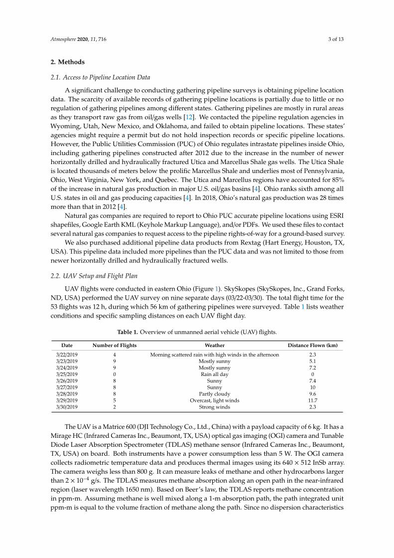
UAV flights were conducted in eastern Ohio (Figure 1). SkySkopes (SkySkopes, Inc., Grand Forks,ND, USA) performed the UAV survey on nine separate days (03/22-03/30). The total flight time for the53 flights was 12 h, during which 56 km of gathering pipelines were surveyed. Table 1 lists weatherconditions and specific sampling distances on each UAV flight day.
Table 1. Overview of unmanned aerial vehicle (UAV) flights.
Date Number of Flights Weather Distance Flown (km)
3/22/2019 4 Morning scattered rain with high winds in the afternoon 2.33/23/2019 9 Mostly sunny 5.13/24/2019 9 Mostly sunny 7.23/25/2019 0 Rain all day 03/26/2019 8 Sunny 7.43/27/2019 8 Sunny 103/28/2019 8 Partly cloudy 9.63/29/2019 5 Overcast, light winds 11.73/30/2019 2 Strong winds 2.3
The UAV is a Matrice 600 (DJI Technology Co., Ltd., China) with a payload capacity of 6 kg. It has aMirage HC (Infrared Cameras Inc., Beaumont, TX, USA) optical gas imaging (OGI) camera and TunableDiode Laser Absorption Spectrometer (TDLAS) methane sensor (Infrared Cameras Inc., Beaumont,TX, USA) on board. Both instruments have a power consumption less than 5 W. The OGI cameracollects radiometric temperature data and produces thermal images using its 640 × 512 InSb array.The camera weighs less than 800 g. It can measure leaks of methane and other hydrocarbons largerthan 2 × 10⁻⁴ g/s. The TDLAS measures methane absorption along an open path in the near-infraredregion (laser wavelength 1650 nm). Based on Beer’s law, the TDLAS reports methane concentrationin ppm-m. Assuming methane is well mixed along a 1-m absorption path, the path integrated unitppm-m is equal to the volume fraction of methane along the path. Since no dispersion characteristics
Atmosphere 2020, 11, 716 4 of 13
are known before the measurement is made, it is difficult to directly convert the ppm-m to commonlyused ppm units. The TDLAS has a time resolution of 1 Hz and can measure methane from a distanceup to 50 m with a resolution of 1 ppm-m. All instruments are synchronized before the campaign.Atmosphere 2020, 11, x FOR PEER REVIEW 4 of 13
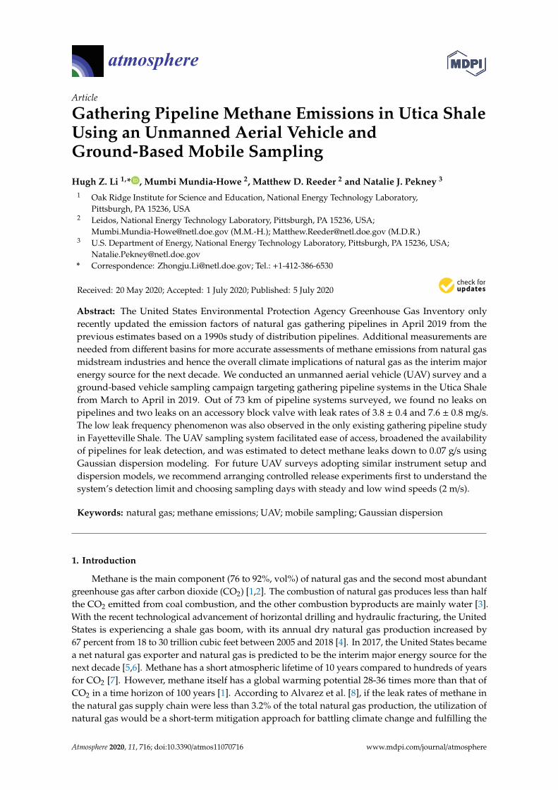
Figure 1. Overview of two survey paths (UAV and ground-based mobile sport utility vehicle (SUV)) in the Utica Shale, specifically in Ohio.
The UAV is a Matrice 600 (DJI Technology Co., Ltd., China) with a payload capacity of 6 kg. It has a Mirage HC (Infrared Cameras Inc., Beaumont, TX, USA) optical gas imaging (OGI) camera and Tunable Diode Laser Absorption Spectrometer (TDLAS) methane sensor (Infrared Cameras Inc., Beaumont, TX, USA) on board. Both instruments have a power consumption less than 5 W. The OGI camera collects radiometric temperature data and produces thermal images using its 640 × 512 InSb array. The camera weighs less than 800 g. It can measure leaks of methane and other hydrocarbons larger than 2 × 10⁻⁴ g/s. The TDLAS measures methane absorption along an open path in the near-infrared region (laser wavelength 1650 nm). Based on Beer’s law, the TDLAS reports methane concentration in ppm-m. Assuming methane is well mixed along a 1-m absorption path, the path integrated unit ppm-m is equal to the volume fraction of methane along the path. Since no dispersion characteristics are known before the measurement is made, it is difficult to directly convert the ppm-m to commonly used ppm units. The TDLAS has a time resolution of 1 Hz and can measure methane from a distance up to 50 m with a resolution of 1 ppm-m. All instruments are synchronized before the campaign.
The factory recommended flight time for a Matrice 600 UAV is 20 minutes. For each flight, the range of the final flight time was from 10 to 20 minutes. The low end of the flight time was mainly due to the rough terrain in eastern Ohio (Figure S1, Supplemental Material) and line-of-sight requirements from the FAA. To create the flight paths, routes from the Google Earth app (Google LLC, Mountainview, CA, USA) were exported to KML files that were then imported to the Litchi software (VC Technology Ltd., London, UK). The Lichi app controlled the speed and altitude of the UAV remotely. The UAV could fly above the ground at user-defined heights regardless of the elevation of the terrain. The factory recommended flight height is between 40 and 50 m. The final range of flight heights was from 42 to 45 m.
Figure 1. Overview of two survey paths (UAV and ground-based mobile sport utility vehicle (SUV)) inthe Utica Shale, specifically in Ohio.
The factory recommended flight time for a Matrice 600 UAV is 20 minutes. For each flight,the range of the final flight time was from 10 to 20 minutes. The low end of the flight time wasmainly due to the rough terrain in eastern Ohio (Figure S1, Supplemental Material) and line-of-sightrequirements from the FAA. To create the flight paths, routes from the Google Earth app (GoogleLLC, Mountainview, CA, USA) were exported to KML files that were then imported to the Litchisoftware (VC Technology Ltd., London, UK). The Lichi app controlled the speed and altitude of theUAV remotely. The UAV could fly above the ground at user-defined heights regardless of the elevationof the terrain. The factory recommended flight height is between 40 and 50 m. The final range of flightheights was from 42 to 45 m.
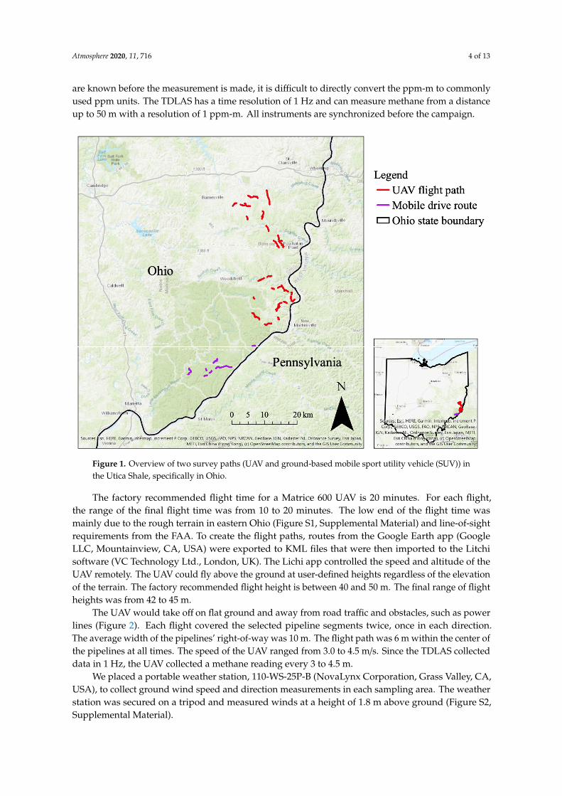
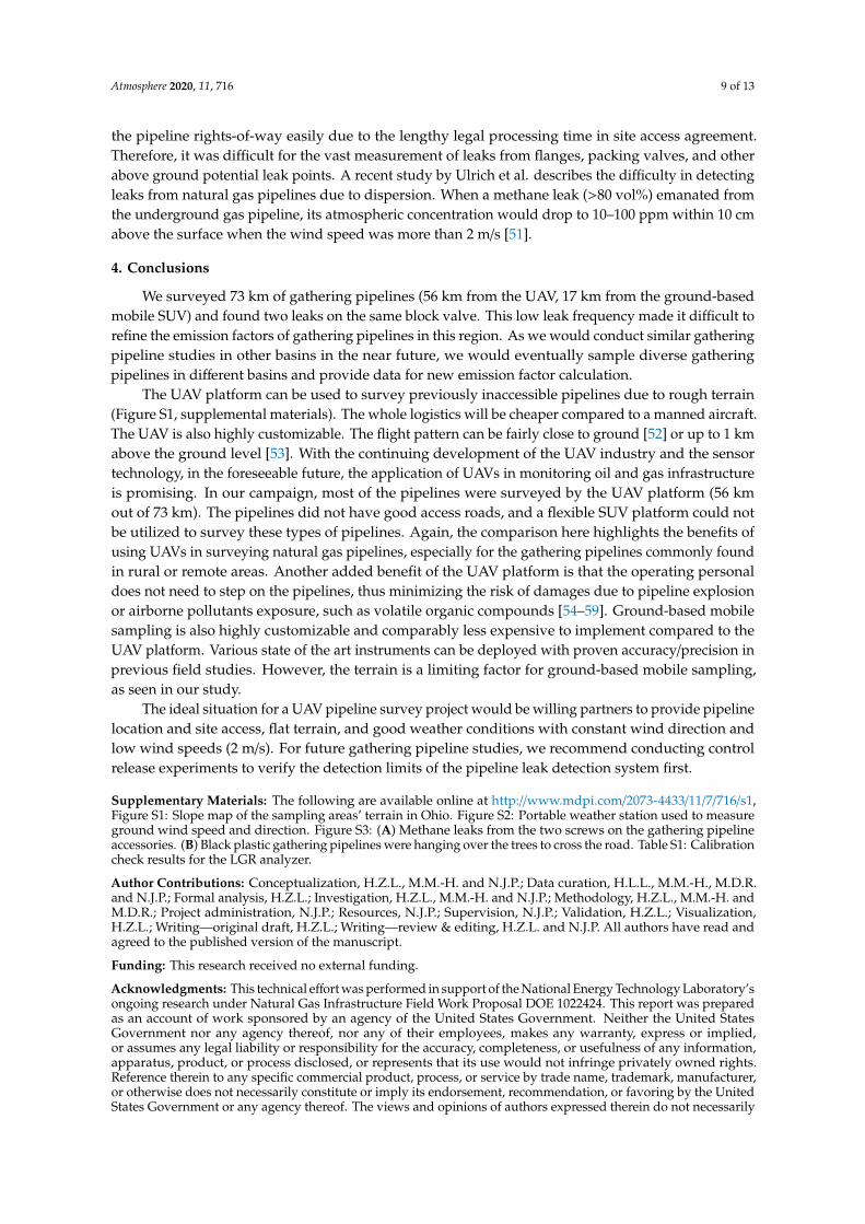
The UAV would take off on flat ground and away from road traffic and obstacles, such as powerlines (Figure 2). Each flight covered the selected pipeline segments twice, once in each direction.The average width of the pipelines’ right-of-way was 10 m. The flight path was 6 m within the center ofthe pipelines at all times. The speed of the UAV ranged from 3.0 to 4.5 m/s. Since the TDLAS collecteddata in 1 Hz, the UAV collected a methane reading every 3 to 4.5 m.
We placed a portable weather station, 110-WS-25P-B (NovaLynx Corporation, Grass Valley, CA,USA), to collect ground wind speed and direction measurements in each sampling area. The weatherstation was secured on a tripod and measured winds at a height of 1.8 m above ground (Figure S2,Supplemental Material).
Atmosphere 2020, 11, 716 5 of 13
Atmosphere 2020, 11, x FOR PEER REVIEW 5 of 13
The UAV would take off on flat ground and away from road traffic and obstacles, such as power lines (Figure 2). Each flight covered the selected pipeline segments twice, once in each direction. The average width of the pipelines’ right-of-way was 10 m. The flight path was 6 m within the center of the pipelines at all times. The speed of the UAV ranged from 3.0 to 4.5 m/s. Since the TDLAS collected data in 1 Hz, the UAV collected a methane reading every 3 to 4.5 m.
We placed a portable weather station, 110-WS-25P-B (NovaLynx Corporation, Grass Valley, CA, USA), to collect ground wind speed and direction measurements in each sampling area. The weather station was secured on a tripod and measured winds at a height of 1.8 m above ground (Figure S2, Supplemental Material).
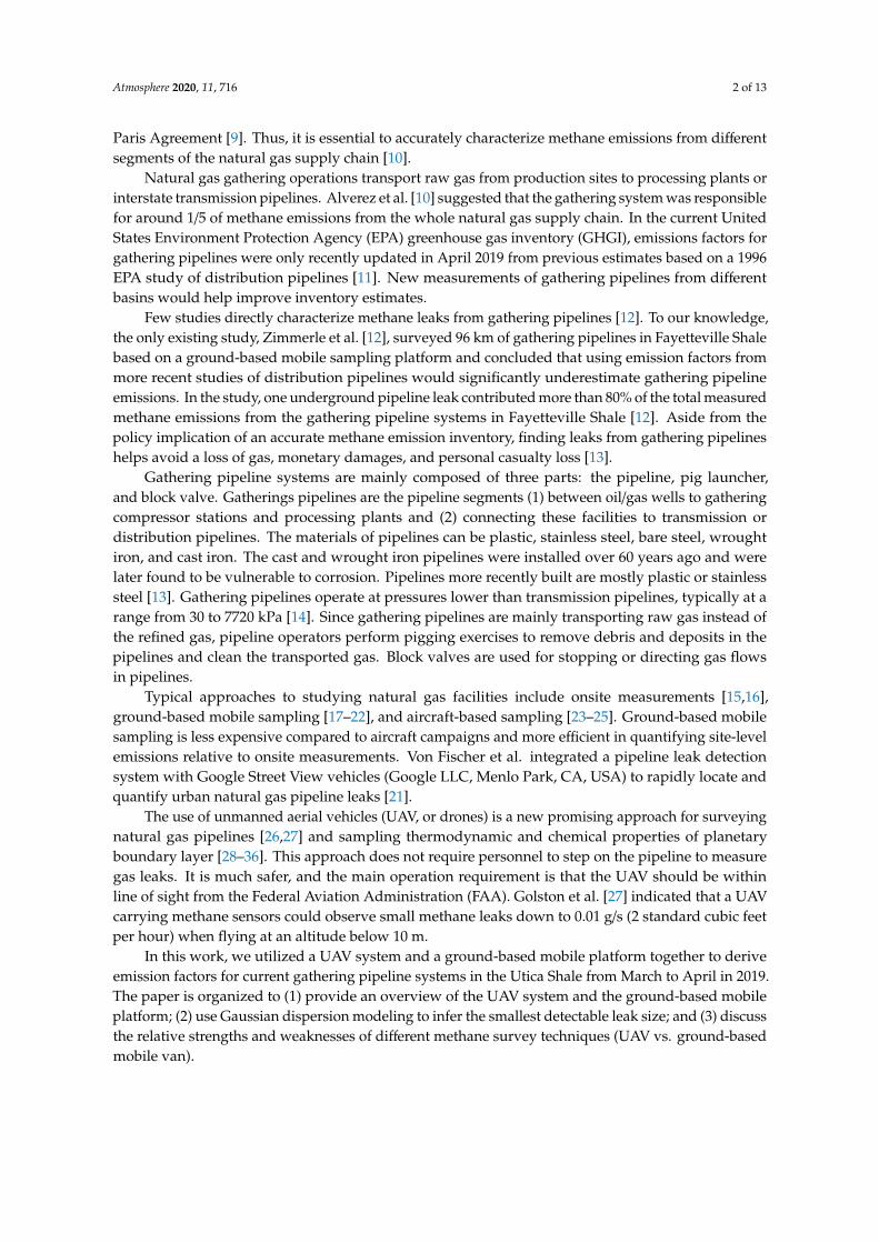
Figure 2. (a) UAV and (b) ground-based sampling vehicle used in this study.
2.3. Ground-Based Vehicle Sampling Setup
A Ford Expedition sport utility vehicle (SUV) was used for the ground-based mobile survey on two trips (04/12/2019 and 04/16/2019). Note that the ground-based mobile survey happened after the UAV flights. In total, 17 km of above-ground pipelines were surveyed.
Although Ohio has 17,000 km of gathering pipelines in total, approximately 160 km are on public lands based on the purchased data products. The mobile survey was restricted to public lands (Wayne National Forest) due to the ease of access as compared to private property. This area of Ohio has rough terrain, with slope degrees frequently larger than 15 degrees (Figure S1, Supplemental Materials).
The details of the mobile sampling approach have been previously described [17]. The cargo area of the vehicle housed an LGR methane analyzer (Los Gatos Research LGR, CA, USA), a Windows laptop for logging data, and a power source for the instruments—a swappable 4–18 V Lithium-ion Bosch battery 6 Ah (Bosch, Blaichach, Germany). The A21TM ANTENNA GPS (Hemisphere GNSS, Scottsdale, AZ) was installed at the top center of the SUV. Wind speed and direction were measured by a weather station, Airmar 200WX, designed for mobile sampling (Airmar, Milford, NH, USA). The Airmar weather station was elevated by a polyvinyl chloride (PVC) pipe to a height of 2.5 m above the ground (Figure 2). This setup helped ensure wind measurements were not affected by vehicle movements [18,37–40]. Our sampling line was a 1/4’’ OD Teflon tube attached to the weather station. The LGR methane analyzer used an oil-free vacuum pump KNF N920 (KNF Neuberger, Inc., Trenton, NJ) for sample collection at a rate of 20 LPM. All instruments were secured so the effects of vehicle motion-induced vibration were minimized. All instruments were synchronized before the survey and reported data in local Eastern time (UTC/GMT-4).
Two researchers participated in each mobile sampling trip, a driver and a co-pilot. The co-pilot checked the analyzer’s methane concentration readings for any elevation larger than 0.5 ppm above background 1.9 ppm [41]. We used methane readings at upwind rural locations as our background [42]. Since some of the pipelines in the forest were above ground, the co-pilot would also point a
(a) (b)
Figure 2. (a) UAV and (b) ground-based sampling vehicle used in this study.
2.3. Ground-Based Vehicle Sampling Setup
A Ford Expedition sport utility vehicle (SUV) was used for the ground-based mobile survey ontwo trips (04/12/2019 and 04/16/2019). Note that the ground-based mobile survey happened after theUAV flights. In total, 17 km of above-ground pipelines were surveyed.
Although Ohio has 17,000 km of gathering pipelines in total, approximately 160 km are on publiclands based on the purchased data products. The mobile survey was restricted to public lands (WayneNational Forest) due to the ease of access as compared to private property. This area of Ohio has roughterrain, with slope degrees frequently larger than 15 degrees (Figure S1, Supplemental Materials).
The details of the mobile sampling approach have been previously described [17]. The cargo areaof the vehicle housed an LGR methane analyzer (Los Gatos Research LGR, CA, USA), a Windowslaptop for logging data, and a power source for the instruments—a swappable 4–18 V Lithium-ionBosch battery 6 Ah (Bosch, Blaichach, Germany). The A21™ ANTENNA GPS (Hemisphere GNSS,Scottsdale, AZ) was installed at the top center of the SUV. Wind speed and direction were measuredby a weather station, Airmar 200WX, designed for mobile sampling (Airmar, Milford, NH, USA).The Airmar weather station was elevated by a polyvinyl chloride (PVC) pipe to a height of 2.5 m abovethe ground (Figure 2). This setup helped ensure wind measurements were not affected by vehiclemovements [18,37–40]. Our sampling line was a 1/4” OD Teflon tube attached to the weather station.The LGR methane analyzer used an oil-free vacuum pump KNF N920 (KNF Neuberger, Inc., Trenton,NJ) for sample collection at a rate of 20 LPM. All instruments were secured so the effects of vehiclemotion-induced vibration were minimized. All instruments were synchronized before the survey andreported data in local Eastern time (UTC/GMT-4).
Two researchers participated in each mobile sampling trip, a driver and a co-pilot. The co-pilotchecked the analyzer’s methane concentration readings for any elevation larger than 0.5 ppm abovebackground 1.9 ppm [41]. We used methane readings at upwind rural locations as our background [42].Since some of the pipelines in the forest were above ground, the co-pilot would also point a handholdmethane detector, the Laser Methane Copter (LMC, Pergam Suisse AG, Switzerland), at the pipeline.When the co-pilot observed methane plume events as registered by the methane analyzer and indicatedon the computer logging software, the driver would pull over and stop the vehicle so that the potentialleak could be located. Once the leak was found, an infrared camera GF320 (FLIR Systems, Wilsonville,OR, USA) was mounted on a tripod to take infrared images and videos. We used the Bacharach Hi Flow®
Sampler to quantify leak rates. Note the LGR methane analyzer provided methane concentrations butnot methane leak rates. For each leak, both high and low flow modes (210 and 150 LPM) were used toget repeated leak rate measurements. Studies have shown that the Bacharach Hi Flow® Sampler couldunderestimate methane emissions due to the sensor failing to switch measurement modes [43]. In our
Atmosphere 2020, 11, 716 6 of 13
practice, we followed the recommendations of Connolly et al. [43], which included shutting down theHi Flow sampler after measuring every single leak and conducting frequent calibration checks. It isunlikely that we were affected by this type of failure.
2.4. Data Quality Control
For the UAV sampling, weather conditions were examined using www.windy.com prior to eachtakeoff. Flights were cancelled or postponed if wind speeds were above 4.5 m/s because, at high winds,leaked methane would disperse rapidly, lowering the chances of detection. Rain and snow were alsoavoided, as the UAV and/or sensors could be damaged. During the UAV campaign (03/22 to 03/30),we observed rain on two days.
As there sometimes were discrepancies between the pipeline location in the Google Earth KMLand the field-observed pipeline rights-of-way or markers, best judgment as to actual pipeline locationwas used to adjust the flight plan. Because the UAV flight paths were designed to pass over eachsegment of the route twice, any leak should be detected at approximately the same location during eachpass. In addition, a ramping followed by a gradual decrease in methane concentration was expectedto be observed as the UAV approached and then departed the leak location. We set the warningthreshold of the TDLAS to be 200 ppm-m, an order of magnitude higher than background (Figure 3).If elevated, ramped-up methane concentration was observed twice around the same spot during oneflight, a second flight would be conducted to collect additional data. The UAV would hover above thepotential leaking spot, and then be lowered to the minimum allowable height to collect the thermalinfrared output and to take videos that would allow for the examination of any vegetation degradation.
Atmosphere 2020, 11, x FOR PEER REVIEW 6 of 13
handhold methane detector, the Laser Methane Copter (LMC, Pergam Suisse AG, Switzerland), at the pipeline. When the co-pilot observed methane plume events as registered by the methane analyzer and indicated on the computer logging software, the driver would pull over and stop the vehicle so that the potential leak could be located. Once the leak was found, an infrared camera GF320 (FLIR Systems, Wilsonville, OR, USA) was mounted on a tripod to take infrared images and videos. We used the Bacharach Hi Flow® Sampler to quantify leak rates. Note the LGR methane analyzer provided methane concentrations but not methane leak rates. For each leak, both high and low flow modes (210 and 150 LPM) were used to get repeated leak rate measurements. Studies have shown that the Bacharach Hi Flow® Sampler could underestimate methane emissions due to the sensor failing to switch measurement modes [43]. In our practice, we followed the recommendations of Connolly et al. [43], which included shutting down the Hi Flow sampler after measuring every single leak and conducting frequent calibration checks. It is unlikely that we were affected by this type of failure.
2.4. Data Quality Control
For the UAV sampling, weather conditions were examined using www.windy.com prior to each takeoff. Flights were cancelled or postponed if wind speeds were above 4.5 m/s because, at high winds, leaked methane would disperse rapidly, lowering the chances of detection. Rain and snow were also avoided, as the UAV and/or sensors could be damaged. During the UAV campaign (03/22 to 03/30), we observed rain on two days.
As there sometimes were discrepancies between the pipeline location in the Google Earth KML and the field-observed pipeline rights-of-way or markers, best judgment as to actual pipeline location was used to adjust the flight plan. Because the UAV flight paths were designed to pass over each segment of the route twice, any leak should be detected at approximately the same location during each pass. In addition, a ramping followed by a gradual decrease in methane concentration was expected to be observed as the UAV approached and then departed the leak location. We set the warning threshold of the TDLAS to be 200 ppm-m, an order of magnitude higher than background (Figure 3). If elevated, ramped-up methane concentration was observed twice around the same spot during one flight, a second flight would be conducted to collect additional data. The UAV would hover above the potential leaking spot, and then be lowered to the minimum allowable height to collect the thermal infrared output and to take videos that would allow for the examination of any vegetation degradation.
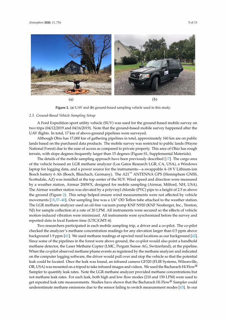
Figure 3. Boxplot of (a) methane readings and (b) wind speeds among all sampling days. The middle line is the median. The top and bottom of the box are the 75th and 25th percentiles. The outer whiskers extend to the most extreme values not yet classified as outliers [44]. The y axis for (a) is log scaled.
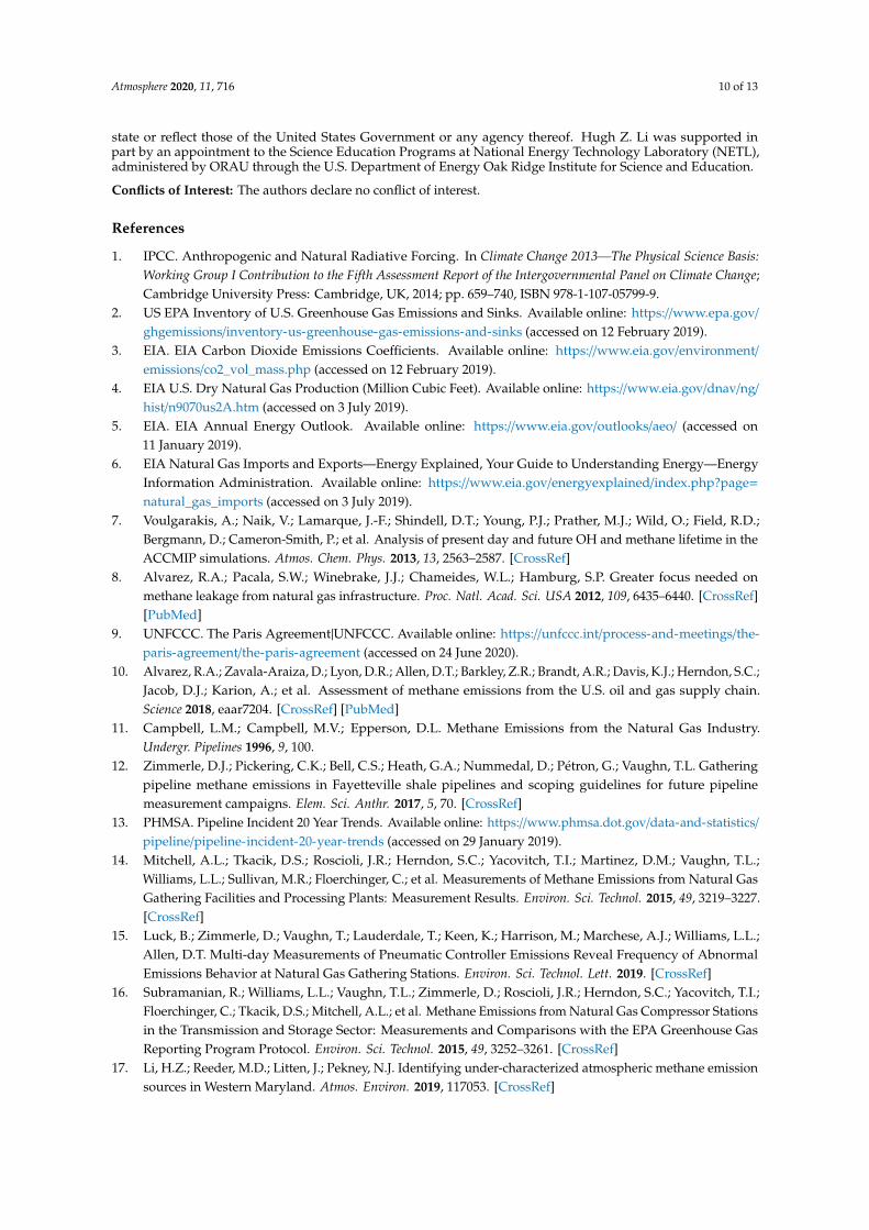
Figure 3. Boxplot of (a) methane readings and (b) wind speeds among all sampling days. The middleline is the median. The top and bottom of the box are the 75th and 25th percentiles. The outer whiskersextend to the most extreme values not yet classified as outliers [44]. The y axis for (a) is log scaled.
As per the manufacturer’s recommendations, a two-point gas calibration was performed forthe Bacharach Hi Flow® Sampler before each mobile sampling trip. The calibration gases were2.5% methane, balance air and 99% methane, balance nitrogen (Heath Consultants, Houston, TX, USA).We chose these two gas compositions as they were included in the calibration menu of the BacharachHi Flow® Sampler.
For ground-based mobile sampling measurements, we filtered the methane dataset for null valuesand any methane values less than 1.5 ppm. The wind data from the Airmar 200 WX were adjustedbased on the in-built data quality indicator. In addition, we conducted residence tests to measure
Atmosphere 2020, 11, 716 7 of 13
traveling time inside the sampling lines before the air samples reached the analyzer. This helped tobetter synchronize the GPS with the methane concentration data.
Calibration checks for the LGR methane analyzer were conducted as per manufacturer’srecommendations. The cavity ring down spectroscopy-based analyzer showed good stability and littledrift during field campaigns [17]. The calibration check results are in Table S1 (Supplemental Material).The analyzer showed good agreement (within 10%) with the methane reference standard (Accuracy:2%, Matheson Tri-Gas, Inc., Bernards, NJ, USA).
2.5. Gaussian Dispersion Modeling
Gaussian dispersion modeling has been used in oil and gas research campaigns to quantify sourceemission rates [17,45]. Assuming a total reflecting ground for methane, a slender plume case, and themeasurement takes place in the plume’s center line, the simplified Gaussian model will be:
c(x, y = 0, z) =q
2πuσyσz×
exp
−(z− h)2
2σ2z
+ exp
−(z + h)2
2σ2z
(1)
where c(x, y, z) is the methane concentration (g/m3) in a specific location (x, y, z), q is the methane leakrate (g/s), u is the mean wind speed (m/s), σy, σz are the dispersion coefficients in the y, z direction (m),and h is the source releasing height above ground (m). We used the Pasquill–Gifford correlations tocalculate the final dispersion coefficients [46].
2.6. Controlled Release Experiment
We conducted a controlled release experiment on 03/28/2019 to verify the leak detection abilityof the methane sensors on the UAV. The weather was sunny, and the wind speeds averaged 4 m/s.We chose an open area for the experiment (Figure S2, Supplemental Materials). To simulate a pipelineleak, we used a 5% methane (vol%) cylinder (Matheson Tri-Gas, Inc., Irving, TX, USA, balance helium,certification accuracy 2%) releasing methane at a flow rate of 5 SLPM (standard liter per minute),as measured by an Alicat mass flow meter (Alicat Scientific, Tucson, AZ, USA). This flow rate wastypical of leaks found on gathering and distribution pipelines [12,47]. Multiple flights were conductedwith the cylinder valve closed or open. The operator flew the drone in the same way as was done forthe actual pipeline survey.
3. Results and Discussion
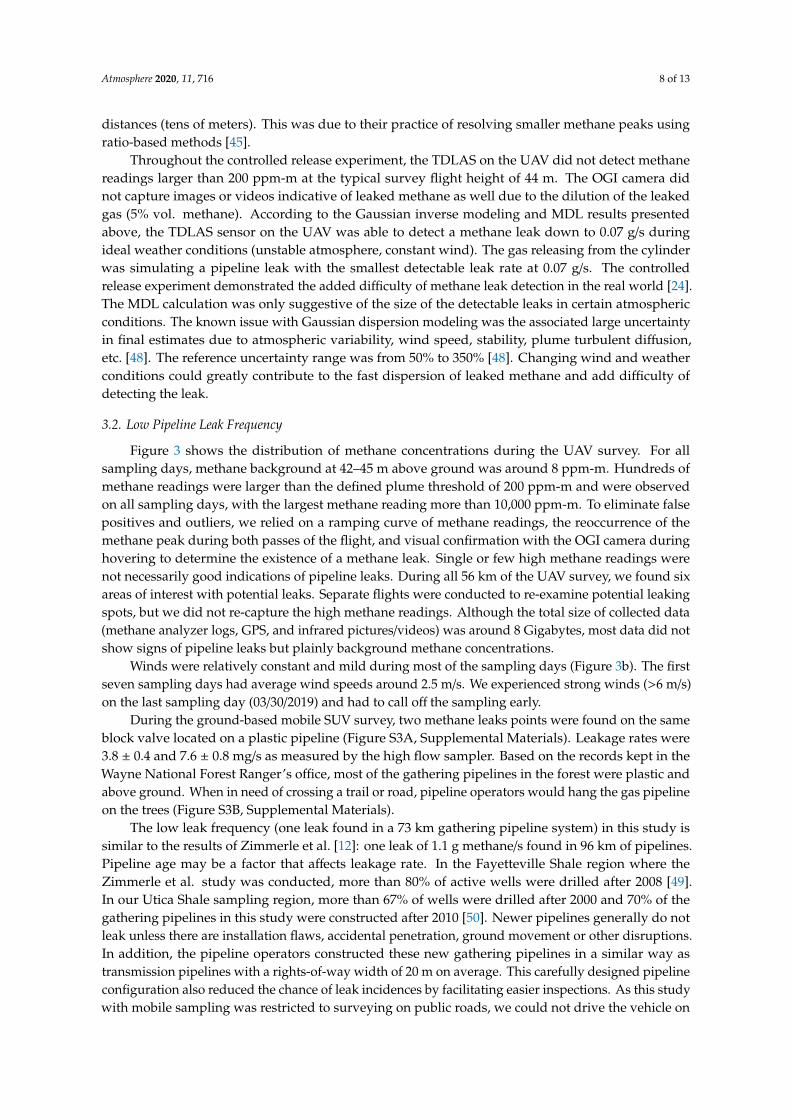
The UAV surveyed 56 km of gathering pipelines and the ground-based SUV survey added another17 km. The UAV surveyed pipelines were all stainless steel based on the Ohio PUC and Rextag datasources. The SUV surveyed 1 km of cast iron and 16 km of plastic pipelines. The diameters of thepipelines ranged from 2.5 to 61.0 cm.
3.1. TDLAS Minimum Detection Limit (MDL)
In our study, the UAV operator SkySkopes used a methane reading of 200 ppm-m as the indicatorof a potential leak. The methane measurements from the UAV were about 4 m from the centerline ofthe pipeline on average. The releasing height for the underground pipeline leaks was at the groundlevel (z = 0 m). The survey area was mostly covered with trees. For a typical wind speed of 2.2 m/s(5 mph, Figure 3), our MDL was 0.07 g/s. This MDL is comparable to those reported in other studies.Subramanian et al. measured different components at compressor stations onsite and reported an MDLof 0.02 g/s [16]. Von Fischer et al. deployed instruments on Google Street View vehicles and focusedon urban natural gas leaks within 20 m of the vehicle [21]. Their setup strategically dismissed smallleaks and had an MDL of 0.5 g/s. Atherton et al. integrated methane analyzers on a mobile samplingplatform and obtained an MDL of 0.06 g/s when they were sampling very close to the natural gas wells(<60 m) [45]. The MDL for this study was 20% larger compared to Atherton et al. at similar measuring
Atmosphere 2020, 11, 716 8 of 13
distances (tens of meters). This was due to their practice of resolving smaller methane peaks usingratio-based methods [45].
Throughout the controlled release experiment, the TDLAS on the UAV did not detect methanereadings larger than 200 ppm-m at the typical survey flight height of 44 m. The OGI camera didnot capture images or videos indicative of leaked methane as well due to the dilution of the leakedgas (5% vol. methane). According to the Gaussian inverse modeling and MDL results presentedabove, the TDLAS sensor on the UAV was able to detect a methane leak down to 0.07 g/s duringideal weather conditions (unstable atmosphere, constant wind). The gas releasing from the cylinderwas simulating a pipeline leak with the smallest detectable leak rate at 0.07 g/s. The controlledrelease experiment demonstrated the added difficulty of methane leak detection in the real world [24].The MDL calculation was only suggestive of the size of the detectable leaks in certain atmosphericconditions. The known issue with Gaussian dispersion modeling was the associated large uncertaintyin final estimates due to atmospheric variability, wind speed, stability, plume turbulent diffusion,etc. [48]. The reference uncertainty range was from 50% to 350% [48]. Changing wind and weatherconditions could greatly contribute to the fast dispersion of leaked methane and add difficulty ofdetecting the leak.
3.2. Low Pipeline Leak Frequency
Figure 3 shows the distribution of methane concentrations during the UAV survey. For allsampling days, methane background at 42–45 m above ground was around 8 ppm-m. Hundreds ofmethane readings were larger than the defined plume threshold of 200 ppm-m and were observedon all sampling days, with the largest methane reading more than 10,000 ppm-m. To eliminate falsepositives and outliers, we relied on a ramping curve of methane readings, the reoccurrence of themethane peak during both passes of the flight, and visual confirmation with the OGI camera duringhovering to determine the existence of a methane leak. Single or few high methane readings werenot necessarily good indications of pipeline leaks. During all 56 km of the UAV survey, we found sixareas of interest with potential leaks. Separate flights were conducted to re-examine potential leakingspots, but we did not re-capture the high methane readings. Although the total size of collected data(methane analyzer logs, GPS, and infrared pictures/videos) was around 8 Gigabytes, most data did notshow signs of pipeline leaks but plainly background methane concentrations.
Winds were relatively constant and mild during most of the sampling days (Figure 3b). The firstseven sampling days had average wind speeds around 2.5 m/s. We experienced strong winds (>6 m/s)on the last sampling day (03/30/2019) and had to call off the sampling early.
During the ground-based mobile SUV survey, two methane leaks points were found on the sameblock valve located on a plastic pipeline (Figure S3A, Supplemental Materials). Leakage rates were3.8 ± 0.4 and 7.6 ± 0.8 mg/s as measured by the high flow sampler. Based on the records kept in theWayne National Forest Ranger’s office, most of the gathering pipelines in the forest were plastic andabove ground. When in need of crossing a trail or road, pipeline operators would hang the gas pipelineon the trees (Figure S3B, Supplemental Materials).
The low leak frequency (one leak found in a 73 km gathering pipeline system) in this study issimilar to the results of Zimmerle et al. [12]: one leak of 1.1 g methane/s found in 96 km of pipelines.Pipeline age may be a factor that affects leakage rate. In the Fayetteville Shale region where theZimmerle et al. study was conducted, more than 80% of active wells were drilled after 2008 [49].In our Utica Shale sampling region, more than 67% of wells were drilled after 2000 and 70% of thegathering pipelines in this study were constructed after 2010 [50]. Newer pipelines generally do notleak unless there are installation flaws, accidental penetration, ground movement or other disruptions.In addition, the pipeline operators constructed these new gathering pipelines in a similar way astransmission pipelines with a rights-of-way width of 20 m on average. This carefully designed pipelineconfiguration also reduced the chance of leak incidences by facilitating easier inspections. As this studywith mobile sampling was restricted to surveying on public roads, we could not drive the vehicle on
Atmosphere 2020, 11, 716 9 of 13
the pipeline rights-of-way easily due to the lengthy legal processing time in site access agreement.Therefore, it was difficult for the vast measurement of leaks from flanges, packing valves, and otherabove ground potential leak points. A recent study by Ulrich et al. describes the difficulty in detectingleaks from natural gas pipelines due to dispersion. When a methane leak (>80 vol%) emanated fromthe underground gas pipeline, its atmospheric concentration would drop to 10–100 ppm within 10 cmabove the surface when the wind speed was more than 2 m/s [51].
4. Conclusions
We surveyed 73 km of gathering pipelines (56 km from the UAV, 17 km from the ground-basedmobile SUV) and found two leaks on the same block valve. This low leak frequency made it difficult torefine the emission factors of gathering pipelines in this region. As we would conduct similar gatheringpipeline studies in other basins in the near future, we would eventually sample diverse gatheringpipelines in different basins and provide data for new emission factor calculation.
The UAV platform can be used to survey previously inaccessible pipelines due to rough terrain(Figure S1, supplemental materials). The whole logistics will be cheaper compared to a manned aircraft.The UAV is also highly customizable. The flight pattern can be fairly close to ground [52] or up to 1 kmabove the ground level [53]. With the continuing development of the UAV industry and the sensortechnology, in the foreseeable future, the application of UAVs in monitoring oil and gas infrastructureis promising. In our campaign, most of the pipelines were surveyed by the UAV platform (56 kmout of 73 km). The pipelines did not have good access roads, and a flexible SUV platform could notbe utilized to survey these types of pipelines. Again, the comparison here highlights the benefits ofusing UAVs in surveying natural gas pipelines, especially for the gathering pipelines commonly foundin rural or remote areas. Another added benefit of the UAV platform is that the operating personaldoes not need to step on the pipelines, thus minimizing the risk of damages due to pipeline explosionor airborne pollutants exposure, such as volatile organic compounds [54–59]. Ground-based mobilesampling is also highly customizable and comparably less expensive to implement compared to theUAV platform. Various state of the art instruments can be deployed with proven accuracy/precision inprevious field studies. However, the terrain is a limiting factor for ground-based mobile sampling,as seen in our study.
The ideal situation for a UAV pipeline survey project would be willing partners to provide pipelinelocation and site access, flat terrain, and good weather conditions with constant wind direction andlow wind speeds (2 m/s). For future gathering pipeline studies, we recommend conducting controlrelease experiments to verify the detection limits of the pipeline leak detection system first.
Supplementary Materials: The following are available online at http://www.mdpi.com/2073-4433/11/7/716/s1,Figure S1: Slope map of the sampling areas’ terrain in Ohio. Figure S2: Portable weather station used to measureground wind speed and direction. Figure S3: (A) Methane leaks from the two screws on the gathering pipelineaccessories. (B) Black plastic gathering pipelines were hanging over the trees to cross the road. Table S1: Calibrationcheck results for the LGR analyzer.
Author Contributions: Conceptualization, H.Z.L., M.M.-H. and N.J.P.; Data curation, H.L.L., M.M.-H., M.D.R.and N.J.P.; Formal analysis, H.Z.L.; Investigation, H.Z.L., M.M.-H. and N.J.P.; Methodology, H.Z.L., M.M.-H. andM.D.R.; Project administration, N.J.P.; Resources, N.J.P.; Supervision, N.J.P.; Validation, H.Z.L.; Visualization,H.Z.L.; Writing—original draft, H.Z.L.; Writing—review & editing, H.Z.L. and N.J.P. All authors have read andagreed to the published version of the manuscript.
Funding: This research received no external funding.
Acknowledgments: This technical effort was performed in support of the National Energy Technology Laboratory’songoing research under Natural Gas Infrastructure Field Work Proposal DOE 1022424. This report was preparedas an account of work sponsored by an agency of the United States Government. Neither the United StatesGovernment nor any agency thereof, nor any of their employees, makes any warranty, express or implied,or assumes any legal liability or responsibility for the accuracy, completeness, or usefulness of any information,apparatus, product, or process disclosed, or represents that its use would not infringe privately owned rights.Reference therein to any specific commercial product, process, or service by trade name, trademark, manufacturer,or otherwise does not necessarily constitute or imply its endorsement, recommendation, or favoring by the UnitedStates Government or any agency thereof. The views and opinions of authors expressed therein do not necessarily
Atmosphere 2020, 11, 716 10 of 13
state or reflect those of the United States Government or any agency thereof. Hugh Z. Li was supported inpart by an appointment to the Science Education Programs at National Energy Technology Laboratory (NETL),administered by ORAU through the U.S. Department of Energy Oak Ridge Institute for Science and Education.
Conflicts of Interest: The authors declare no conflict of interest.
References
1. IPCC. Anthropogenic and Natural Radiative Forcing. In Climate Change 2013—The Physical Science Basis:Working Group I Contribution to the Fifth Assessment Report of the Intergovernmental Panel on Climate Change;Cambridge University Press: Cambridge, UK, 2014; pp. 659–740, ISBN 978-1-107-05799-9.
2. US EPA Inventory of U.S. Greenhouse Gas Emissions and Sinks. Available online: https://www.epa.gov/
ghgemissions/inventory-us-greenhouse-gas-emissions-and-sinks (accessed on 12 February 2019).3. EIA. EIA Carbon Dioxide Emissions Coefficients. Available online: https://www.eia.gov/environment/
emissions/co2_vol_mass.php (accessed on 12 February 2019).4. EIA U.S. Dry Natural Gas Production (Million Cubic Feet). Available online: https://www.eia.gov/dnav/ng/
hist/n9070us2A.htm (accessed on 3 July 2019).5. EIA. EIA Annual Energy Outlook. Available online: https://www.eia.gov/outlooks/aeo/ (accessed on
11 January 2019).6. EIA Natural Gas Imports and Exports—Energy Explained, Your Guide to Understanding Energy—Energy
Information Administration. Available online: https://www.eia.gov/energyexplained/index.php?page=
natural_gas_imports (accessed on 3 July 2019).7. Voulgarakis, A.; Naik, V.; Lamarque, J.-F.; Shindell, D.T.; Young, P.J.; Prather, M.J.; Wild, O.; Field, R.D.;
Bergmann, D.; Cameron-Smith, P.; et al. Analysis of present day and future OH and methane lifetime in theACCMIP simulations. Atmos. Chem. Phys. 2013, 13, 2563–2587. [CrossRef]
8. Alvarez, R.A.; Pacala, S.W.; Winebrake, J.J.; Chameides, W.L.; Hamburg, S.P. Greater focus needed onmethane leakage from natural gas infrastructure. Proc. Natl. Acad. Sci. USA 2012, 109, 6435–6440. [CrossRef][PubMed]
9. UNFCCC. The Paris Agreement|UNFCCC. Available online: https://unfccc.int/process-and-meetings/the-paris-agreement/the-paris-agreement (accessed on 24 June 2020).
10. Alvarez, R.A.; Zavala-Araiza, D.; Lyon, D.R.; Allen, D.T.; Barkley, Z.R.; Brandt, A.R.; Davis, K.J.; Herndon, S.C.;Jacob, D.J.; Karion, A.; et al. Assessment of methane emissions from the U.S. oil and gas supply chain.Science 2018, eaar7204. [CrossRef] [PubMed]
11. Campbell, L.M.; Campbell, M.V.; Epperson, D.L. Methane Emissions from the Natural Gas Industry.Undergr. Pipelines 1996, 9, 100.
12. Zimmerle, D.J.; Pickering, C.K.; Bell, C.S.; Heath, G.A.; Nummedal, D.; Pétron, G.; Vaughn, T.L. Gatheringpipeline methane emissions in Fayetteville shale pipelines and scoping guidelines for future pipelinemeasurement campaigns. Elem. Sci. Anthr. 2017, 5, 70. [CrossRef]
13. PHMSA. Pipeline Incident 20 Year Trends. Available online: https://www.phmsa.dot.gov/data-and-statistics/pipeline/pipeline-incident-20-year-trends (accessed on 29 January 2019).
14. Mitchell, A.L.; Tkacik, D.S.; Roscioli, J.R.; Herndon, S.C.; Yacovitch, T.I.; Martinez, D.M.; Vaughn, T.L.;Williams, L.L.; Sullivan, M.R.; Floerchinger, C.; et al. Measurements of Methane Emissions from Natural GasGathering Facilities and Processing Plants: Measurement Results. Environ. Sci. Technol. 2015, 49, 3219–3227.[CrossRef]
15. Luck, B.; Zimmerle, D.; Vaughn, T.; Lauderdale, T.; Keen, K.; Harrison, M.; Marchese, A.J.; Williams, L.L.;Allen, D.T. Multi-day Measurements of Pneumatic Controller Emissions Reveal Frequency of AbnormalEmissions Behavior at Natural Gas Gathering Stations. Environ. Sci. Technol. Lett. 2019. [CrossRef]
16. Subramanian, R.; Williams, L.L.; Vaughn, T.L.; Zimmerle, D.; Roscioli, J.R.; Herndon, S.C.; Yacovitch, T.I.;Floerchinger, C.; Tkacik, D.S.; Mitchell, A.L.; et al. Methane Emissions from Natural Gas Compressor Stationsin the Transmission and Storage Sector: Measurements and Comparisons with the EPA Greenhouse GasReporting Program Protocol. Environ. Sci. Technol. 2015, 49, 3252–3261. [CrossRef]
17. Li, H.Z.; Reeder, M.D.; Litten, J.; Pekney, N.J. Identifying under-characterized atmospheric methane emissionsources in Western Maryland. Atmos. Environ. 2019, 117053. [CrossRef]
Atmosphere 2020, 11, 716 11 of 13
18. Li, H.Z.; Dallmann, T.R.; Li, X.; Gu, P.; Presto, A.A. Urban Organic Aerosol Exposure: Spatial Variations inComposition and Source Impacts. Environ. Sci. Technol. 2017. [CrossRef]
19. Omara, M.; Zimmerman, N.; Sullivan, M.R.; Li, X.; Ellis, A.; Cesa, R.; Subramanian, R.; Presto, A.A.;Robinson, A.L. Methane Emissions from Natural Gas Production Sites in the United States: Data Synthesisand National Estimate. Environ. Sci. Technol. 2018, 52, 12915–12925. [CrossRef] [PubMed]
20. Omara, M.; Sullivan, M.R.; Li, X.; Subramanian, R.; Robinson, A.L.; Presto, A.A. Methane Emissions fromConventional and Unconventional Natural Gas Production Sites in the Marcellus Shale Basin. Environ. Sci.Technol. 2016, 50, 2099–2107. [CrossRef] [PubMed]
21. von Fischer, J.C.; Cooley, D.; Chamberlain, S.; Gaylord, A.; Griebenow, C.J.; Hamburg, S.P.; Salo, J.;Schumacher, R.; Theobald, D.; Ham, J. Rapid, Vehicle-Based Identification of Location and Magnitude ofUrban Natural Gas Pipeline Leaks. Environ. Sci. Technol. 2017, 51, 4091–4099. [CrossRef] [PubMed]
22. Ye, Q.; Gu, P.; Li, H.Z.; Robinson, E.S.; Lipsky, E.; Kaltsonoudis, C.; Lee, A.K.Y.; Apte, J.S.; Robinson, A.L.;Sullivan, R.C.; et al. Spatial Variability of Sources and Mixing State of Atmospheric Particles in a MetropolitanArea. Environ. Sci. Technol. 2018, 52, 6807–6815. [CrossRef]
23. Ren, X.; Salmon, O.E.; Hansford, J.R.; Ahn, D.; Hall, D.; Benish, S.E.; Stratton, P.R.; He, H.; Sahu, S.;Grimes, C.; et al. Methane Emissions From the Baltimore-Washington Area Based on Airborne Observations:Comparison to Emissions Inventories. J. Geophys. Res. Atmos. 2018, 123, 8869–8882. [CrossRef]
24. Cui, Y.Y.; Henze, D.K.; Brioude, J.; Angevine, W.M.; Liu, Z.; Bousserez, N.; Guerrette, J.; McKeen, S.A.;Peischl, J.; Yuan, B.; et al. Inversion Estimates of Lognormally Distributed Methane Emission Rates From theHaynesville-Bossier Oil and Gas Production Region Using Airborne Measurements. J. Geophys. Res. Atmos.2019, 124, 3520–3531. [CrossRef]
25. Vaughn, T.L.; Bell, C.S.; Pickering, C.K.; Schwietzke, S.; Heath, G.A.; Pétron, G.; Zimmerle, D.J.; Schnell, R.C.;Nummedal, D. Temporal variability largely explains top-down/bottom-up difference in methane emissionestimates from a natural gas production region. Proc. Natl. Acad. Sci. USA 2018, 115, 11712–11717. [CrossRef]
26. Yang, S.; Talbot, R.; Frish, M.; Golston, L.; Aubut, N.; Zondlo, M.; Gretencord, C.; McSpiritt, J. Natural GasFugitive Leak Detection Using an Unmanned Aerial Vehicle: Measurement System Description and MassBalance Approach. Atmosphere 2018, 9, 383. [CrossRef]
27. Golston, L.; Aubut, N.; Frish, M.; Yang, S.; Talbot, R.; Gretencord, C.; McSpiritt, J.; Zondlo, M. Natural GasFugitive Leak Detection Using an Unmanned Aerial Vehicle: Localization and Quantification of EmissionRate. Atmosphere 2018, 9, 333. [CrossRef]
28. Barbieri, L.; Kral, S.; Bailey, S.; Frazier, A.; Jacob, J.; Reuder, J.; Brus, D.; Chilson, P.; Crick, C.; Detweiler, C.;et al. Intercomparison of Small Unmanned Aircraft System (sUAS) Measurements for Atmospheric Scienceduring the LAPSE-RATE Campaign. Sensors 2019, 19, 2179. [CrossRef]
29. Lee, T.; Buban, M.; Dumas, E.; Baker, C. On the Use of Rotary-Wing Aircraft to Sample Near-SurfaceThermodynamic Fields: Results from Recent Field Campaigns. Sensors 2018, 19, 10. [CrossRef] [PubMed]
30. Nolan, P.; McClelland, H.; Woolsey, C.; Ross, S. A Method for Detecting Atmospheric Lagrangian CoherentStructures Using a Single Fixed-Wing Unmanned Aircraft System. Sensors 2019, 19, 1607. [CrossRef][PubMed]
31. Rautenberg, A.; Graf, M.; Wildmann, N.; Platis, A.; Bange, J. Reviewing Wind Measurement Approaches forFixed-Wing Unmanned Aircraft. Atmosphere 2018, 9, 422. [CrossRef]
32. Rautenberg, A.; Schön, M.; Zum Berge, K.; Mauz, M.; Manz, P.; Platis, A.; van Kesteren, B.; Suomi, I.; Kral, S.T.;Bange, J. The Multi-Purpose Airborne Sensor Carrier MASC-3 for Wind and Turbulence Measurements inthe Atmospheric Boundary Layer. Sensors 2019, 19, 2292. [CrossRef]
33. Schuyler, T.; Guzman, M. Unmanned Aerial Systems for Monitoring Trace Tropospheric Gases.Atmosphere 2017, 8, 206. [CrossRef]
34. Schuyler, T.J.; Bailey, S.C.C.; Guzman, M.I. Monitoring Tropospheric Gases with Small Unmanned AerialSystems (sUAS) during the Second CLOUDMAP Flight Campaign. Atmosphere 2019, 10, 434. [CrossRef]
35. Schuyler, T.J.; Gohari, S.M.I.; Pundsack, G.; Berchoff, D.; Guzman, M.I. Using a Balloon-Launched UnmannedGlider to Validate Real-Time WRF Modeling. Sensors 2019, 19, 1914. [CrossRef]
36. Witte, B.; Singler, R.; Bailey, S. Development of an Unmanned Aerial Vehicle for the Measurement ofTurbulence in the Atmospheric Boundary Layer. Atmosphere 2017, 8, 195. [CrossRef]
Atmosphere 2020, 11, 716 12 of 13
37. Gu, P.; Li, H.Z.; Ye, Q.; Robinson, E.S.; Apte, J.S.; Robinson, A.L.; Presto, A.A. Intracity Variability ofParticulate Matter Exposure Is Driven by Carbonaceous Sources and Correlated with Land-Use Variables.Environ. Sci. Technol. 2018, 52, 11545–11554. [CrossRef]
38. Li, H.Z.; Gu, P.; Ye, Q.; Zimmerman, N.; Robinson, E.S.; Subramanian, R.; Apte, J.S.; Robinson, A.L.; Presto, A.A.Spatially dense air pollutant sampling: Implications of spatial variability on the representativeness ofstationary air pollutant monitors. Atmos. Environ. X 2019, 100012. [CrossRef]
39. Li, H.Z.; Dallmann, T.R.; Gu, P.; Presto, A.A. Application of mobile sampling to investigate spatial variationin fine particle composition. Atmos. Environ. 2016, 142, 71–82. [CrossRef]
40. Robinson, E.S.; Gu, P.; Ye, Q.; Li, H.Z.; Shah, R.U.; Apte, J.S.; Robinson, A.L.; Presto, A.A. Restaurant Impactson Outdoor Air Quality: Elevated Organic Aerosol Mass from Restaurant Cooking with Neighborhood-ScalePlume Extents. Environ. Sci. Technol. 2018. [CrossRef]
41. Phillips, N.G.; Ackley, R.; Crosson, E.R.; Down, A.; Hutyra, L.R.; Brondfield, M.; Karr, J.D.; Zhao, K.;Jackson, R.B. Mapping urban pipeline leaks: Methane leaks across Boston. Environ. Pollut. 2013, 173, 1–4.[CrossRef] [PubMed]
42. Saha, P.K.; Zimmerman, N.; Malings, C.; Hauryliuk, A.; Li, Z.; Snell, L.; Subramanian, R.; Lipsky, E.; Apte, J.S.;Robinson, A.L.; et al. Quantifying high-resolution spatial variations and local source impacts of urbanultrafine particle concentrations. Sci. Total Environ. 2019, 655, 473–481. [CrossRef] [PubMed]
43. Connolly, J.I.; Robinson, R.A.; Gardiner, T.D. Assessment of the Bacharach Hi Flow® Sampler characteristicsand potential failure modes when measuring methane emissions. Measurement 2019, 145, 226–233. [CrossRef]
44. McGill, R.; Tukey, J.W.; Larsen, W.A. Variations of Box Plots. Am. Stat. 1978, 32, 12. [CrossRef]45. Atherton, E.; Risk, D.; Fougère, C.; Lavoie, M.; Marshall, A.; Werring, J.; Williams, J.P.; Minions, C.
Mobile measurement of methane emissions from natural gas developments in northeastern British Columbia,Canada. Atmos. Chem. Phys. 2017, 17, 12405–12420. [CrossRef]
46. Turner, D.B. Workbook of Atmospheric Dispersion Estimates: An Introduction to Dispersion Modeling, Second Edition;CRC Press: Boca Raton, FL, USA, 1994; ISBN 978-1-56670-023-8.
47. Lamb, B.K.; Edburg, S.L.; Ferrara, T.W.; Howard, T.; Harrison, M.R.; Kolb, C.E.; Townsend-Small, A.; Dyck, W.;Possolo, A.; Whetstone, J.R. Direct Measurements Show Decreasing Methane Emissions from Natural GasLocal Distribution Systems in the United States. Environ. Sci. Technol. 2015, 49, 5161–5169. [CrossRef]
48. Caulton, D.R.; Li, Q.; Bou-Zeid, E.; Fitts, J.P.; Golston, L.M.; Pan, D.; Lu, J.; Lane, H.M.; Buchholz, B.; Guo, X.;et al. Quantifying uncertainties from mobile-laboratory-derived emissions of well pads using inverseGaussian methods. Atmos. Chem. Phys. 2018, 18, 15145–15168. [CrossRef]
49. AOGC. 2018 Arkansas Production & Well Data. Available online: http://www.aogc2.state.ar.us/welldata/
default.aspx (accessed on 5 July 2019).50. Ohio DNR Ohio Oil & Gas Well Production Numbers. Available online: http://oilandgas.ohiodnr.gov/
production#COMB (accessed on 5 July 2019).51. Ulrich, B.A.; Mitton, M.; Lachenmeyer, E.; Hecobian, A.; Zimmerle, D.; Smits, K.M. Natural Gas Emissions
from Underground Pipelines and Implications for Leak Detection. Environ. Sci. Technol. Lett. 2019. [CrossRef]52. Nolan, P.; Pinto, J.; González-Rocha, J.; Jensen, A.; Vezzi, C.; Bailey, S.; de Boer, G.; Diehl, C.; Laurence, R.;
Powers, C.; et al. Coordinated Unmanned Aircraft System (UAS) and Ground-Based Weather Measurementsto Predict Lagrangian Coherent Structures (LCSs). Sensors 2018, 18, 4448. [CrossRef] [PubMed]
53. Alaoui-Sosse, S.; Durand, P.; Medina, P.; Pastor, P.; Lothon, M.; Cernov, I. OVLI-TA: An Unmanned AerialSystem for Measuring Profiles and Turbulence in the Atmospheric Boundary Layer. Sensors 2019, 19, 581.[CrossRef] [PubMed]
54. Li, H.Z.; Reeder, M.D.; Pekney, N.J. Quantifying source contributions of volatile organic compounds underhydraulic fracking moratorium. Sci. Total Environ. 2020, 139322. [CrossRef] [PubMed]
55. Gu, P.; Dallmann, T.R.; Li, H.Z.; Tan, Y.; Presto, A.A. Quantifying Urban Spatial Variations of AnthropogenicVOC Concentrations and Source Contributions with a Mobile Sampling Platform. Int. J. Environ. Res. Public.Health 2019, 16, 1632. [CrossRef]
56. Shah, R.U.; Coggon, M.M.; Gkatzelis, G.I.; McDonald, B.C.; Tasoglou, A.; Huber, H.; Gilman, J.; Warneke, C.;Robinson, A.L.; Presto, A.A. Urban Oxidation Flow Reactor Measurements Reveal Significant SecondaryOrganic Aerosol Contributions from Volatile Emissions of Emerging Importance. Environ. Sci. Technol. 2020,acs.est.9b06531. [CrossRef] [PubMed]
Atmosphere 2020, 11, 716 13 of 13
57. Ye, Q.; Li, H.Z.; Gu, P.; Robinson, E.S.; Apte, J.S.; Sullivan, R.C.; Robinson, A.L.; Donahue, N.M.; Presto, A.A.Moving beyond Fine Particle Mass: High-Spatial Resolution Exposure to Source-Resolved AtmosphericParticle Number and Chemical Mixing State. Environ. Health Perspect. 2020, 128, 017009. [CrossRef]
58. Donahue, N.M.; Posner, L.N.; Westervelt, D.M.; Li, Z.; Shrivastava, M.; Presto, A.A.; Sullivan, R.C.; Adams, P.J.;Pandis, S.N.; Robinson, A.L. Where Did This Particle Come From? Sources of Particle Number and Mass forHuman Exposure Estimates. In Issues in Environmental Science and Technology; Harrison, R.M., Hester, R.E.,Querol, X., Eds.; Royal Society of Chemistry: Cambridge, UK, 2016; pp. 35–71, ISBN 978-1-78262-491-2.
59. Robinson, E.S.; Shah, R.U.; Messier, K.; Gu, P.; Li, H.Z.; Apte, J.S.; Robinson, A.L.; Presto, A.A.Land-Use Regression Modeling of Source-Resolved Fine Particulate Matter Components from MobileSampling. Environ. Sci. Technol. 2019, 53, 8925–8937. [CrossRef]
© 2020 by the authors. Licensee MDPI, Basel, Switzerland. This article is an open accessarticle distributed under the terms and conditions of the Creative Commons Attribution(CC BY) license (http://creativecommons.org/licenses/by/4.0/).