Offline and Online Adaboost for Detecting Anatomic Structures

by

Hong Wu

A Thesis Presented in Partial Fulfillmentof the Requirements for the Degree

Master of Science

Approved July 2011 by theGraduate Supervisory Committee:

Jianming Liang, ChairGerald FarinJieping Ye

ARIZONA STATE UNIVERSITY

August 2011

ABSTRACT

Detecting anatomical structures, such as the carina, the pulmonary trunk

and the aortic arch, is an important step in designing a CAD system of detection

Pulmonary Embolism.

The presented CAD system gets rid of the high-level prior defined knowledge

to become a system which can easily extend to detect other anatomic structures.

The system is based on a machine learning algorithm — AdaBoost and a general

feature — Haar. This study emphasizes on off-line and on-line AdaBoost learn-

ing. And in on-line AdaBoost, the thesis further deals with extremely imbalanced

condition.

The thesis first reviews several knowledge-based detection methods, which

are relied on human being’s understanding of the relationship between anatomic

structures. Then the thesis introduces a classic off-line AdaBoost learning. The

thesis applies different cascading scheme, namely multi-exit cascading scheme.

The comparison between the two methods will be provided and discussed.

Both of the off-line AdaBoost methods have problems in memory usage and

time consuming. Off-line AdaBoost methods need to store all the training samples

and the dataset need to be set before training. The dataset cannot be enlarged

dynamically. Different training dataset requires retraining the whole process. The

retraining is very time consuming and even not realistic.

To deal with the shortcomings of off-line learning, the study exploited on-

line AdaBoost learning approach. The thesis proposed a novel pool based on-line

method with Kalman filters and histogram to better represent the distribution of the

samples’ weight. Analysis of the performance, the stability and the computational

complexity will be provided in the thesis.

i

Furthermore, the original on-line AdaBoost performs badly in imbalanced

conditions, which occur frequently in medical image processing. In image dataset,

positive samples are limited and negative samples are countless. A novel Self-

Adaptive Asymmetric On-line Boosting method is presented. The method utilized a

new asymmetric loss criterion with self-adaptability according to the ratio of exposed

positive and negative samples and it has an advanced rule to update sample’s

importance weight taking account of both classification result and sample’s label.

Compared to traditional on-line AdaBoost Learning method, the new method can

achieve far more accuracy in imbalanced conditions.

ii

DEDICATION

Dedicated the work to my family

iii

ACKNOWLEDGEMENTS

I would like to thank my advisor, Dr. Jianming Liang, for his continued and patient

guidance during the study of the whole Master degree. Dr. Liang’s vision and

construction criticisms have helped me accomplish my goals.

Special thanks to Deng Kun, Nima Tajbakhsh and Wenzhe Xue for helping me

during the various stages of my researchs.

My deepest gratitude to my family’s constant help.

iv

TABLE OF CONTENTS

Page

TABLE OF CONTENTS . . . . . . . . . . . . . . . . . . . . . . . . . . . . . v

LIST OF TABLES . . . . . . . . . . . . . . . . . . . . . . . . . . . . . . . . . vii

LIST OF FIGURES . . . . . . . . . . . . . . . . . . . . . . . . . . . . . . . . viii

CHAPTER . . . . . . . . . . . . . . . . . . . . . . . . . . . . . . . . . . . . . 1

1 INTRODUCTION . . . . . . . . . . . . . . . . . . . . . . . . . . . . . . . 1

1.1 Background . . . . . . . . . . . . . . . . . . . . . . . . . . . . . . . 1

1.2 Motivation . . . . . . . . . . . . . . . . . . . . . . . . . . . . . . . . 2

1.3 Prototype Structure . . . . . . . . . . . . . . . . . . . . . . . . . . . 3

1.4 Thesis Organization . . . . . . . . . . . . . . . . . . . . . . . . . . . 4

2 OFF-LINE ADABOOST . . . . . . . . . . . . . . . . . . . . . . . . . . . . 6

2.1 Review of the Existed Methods Besides Boosting . . . . . . . . . . . 6

2.2 Review of the Existed Methods . . . . . . . . . . . . . . . . . . . . . 9

Haar Feature and Integral Image . . . . . . . . . . . . . . . . . . . . 10

Viola’s Cascading Scheme . . . . . . . . . . . . . . . . . . . . . . . 11

2.3 Proposed Method: AdaBoost with Multi-exit Cascading Scheme . . . 12

2.4 Experiment and Results . . . . . . . . . . . . . . . . . . . . . . . . 13

Data Preparation . . . . . . . . . . . . . . . . . . . . . . . . . . . . 13

AdaBoost without Cascade . . . . . . . . . . . . . . . . . . . . . . . 17

Viola’s AdaBoost Cascading Scheme . . . . . . . . . . . . . . . . . 17

Multi-exit AdaBoost Cascading Scheme . . . . . . . . . . . . . . . . 17

AdaBoost with More Representative Negative Samples . . . . . . . 19

2.5 Discussion . . . . . . . . . . . . . . . . . . . . . . . . . . . . . . . . 19

3 ON-LINE ADABOOST . . . . . . . . . . . . . . . . . . . . . . . . . . . . 26

3.1 Review of the Existed Methods . . . . . . . . . . . . . . . . . . . . . 27

3.2 Proposed method: Pool Based On-line AdaBoost . . . . . . . . . . . 29

Histogram Weak Learner . . . . . . . . . . . . . . . . . . . . . . . . 30

v

Chapter PageLearning Process . . . . . . . . . . . . . . . . . . . . . . . . . . . . 31

3.3 Experiment and Result . . . . . . . . . . . . . . . . . . . . . . . . . 33

3.4 Discussion . . . . . . . . . . . . . . . . . . . . . . . . . . . . . . . . 34

Stability . . . . . . . . . . . . . . . . . . . . . . . . . . . . . . . . . 34

Comparison between Kalman and Histogram . . . . . . . . . . . . . 36

4 ON-LINE ASYMMETRIC ADABOOST . . . . . . . . . . . . . . . . . . . . 38

4.1 Review of the Existed Methods . . . . . . . . . . . . . . . . . . . . . 38

4.2 Self-Adaptive Asymmetric On-line Boosting (SAAOB) . . . . . . . . . 39

Contribution . . . . . . . . . . . . . . . . . . . . . . . . . . . . . . . 39

Asymmetric Loss Criterion . . . . . . . . . . . . . . . . . . . . . . . 40

Sample’s Importance Weight . . . . . . . . . . . . . . . . . . . . . . 42

4.3 Experiments and results . . . . . . . . . . . . . . . . . . . . . . . . 43

Datasets . . . . . . . . . . . . . . . . . . . . . . . . . . . . . . . . . 43

Training Process . . . . . . . . . . . . . . . . . . . . . . . . . . . . 44

Testing Process and Performance Criterion . . . . . . . . . . . . . . 44

Comparison . . . . . . . . . . . . . . . . . . . . . . . . . . . . . . . 44

4.4 Discussion . . . . . . . . . . . . . . . . . . . . . . . . . . . . . . . . 47

5 CONCLUSION . . . . . . . . . . . . . . . . . . . . . . . . . . . . . . . . 51

REFERENCE . . . . . . . . . . . . . . . . . . . . . . . . . . . . . . . . . . . 53

vi

LIST OF TABLES

Table Page

1.1 Incidence and Mortality of Different Diseases . . . . . . . . . . . . . . . 2

2.1 Experiment Results of Several Off-line AdaBoost Approaches . . . . . . 19

2.2 Pseudo Code of AdaBoost, RealBoost and GentleBoost . . . . . . . . . 20

3.1 Pseudo Code of Proposed On-line AdaBoost Approach . . . . . . . . . 32

3.2 Experiment Results of Several On-line AdaBoost Approaches . . . . . . 33

4.1 Pseudo Code of Self-Adaptive Asymmetric On-line Boosting Approach . 41

4.2 Comparison between Symmetric and Asymmetric Approaches at Sam-

ple Level . . . . . . . . . . . . . . . . . . . . . . . . . . . . . . . . . . . 45

4.3 Comparison between Symmetric and Asymmetric Approaches at Patient

Level . . . . . . . . . . . . . . . . . . . . . . . . . . . . . . . . . . . . . 49

4.4 Comparison between Symmetric and Asymmetric Approaches at Patient

Level by Increasing the Number of Negative Samples . . . . . . . . . . 50

vii

LIST OF FIGURES

Figure Page

1.1 Illustration of the Incidence and Mortality in Table 1.1 . . . . . . . . . . 2

1.2 Pulmonary Trunk and Central Pulmonary Embolism . . . . . . . . . . . 3

1.3 Three Anatomical Structures . . . . . . . . . . . . . . . . . . . . . . . . 4

1.4 Chart Flow of the Prototype . . . . . . . . . . . . . . . . . . . . . . . . 5

2.1 Grouping Features . . . . . . . . . . . . . . . . . . . . . . . . . . . . . 6

2.2 High-Level Knowledge Based Method . . . . . . . . . . . . . . . . . . . 8

2.3 Template Matching . . . . . . . . . . . . . . . . . . . . . . . . . . . . . 8

2.4 Anatomy Based Detection on the Pulmonary Trunk . . . . . . . . . . . . 9

2.5 Integral Image . . . . . . . . . . . . . . . . . . . . . . . . . . . . . . . . 11

2.6 Haar Feature . . . . . . . . . . . . . . . . . . . . . . . . . . . . . . . . 11

2.7 Viola’s AdaBoost Cascading Scheme . . . . . . . . . . . . . . . . . . . 12

2.8 Multi-exit Cascading Scheme . . . . . . . . . . . . . . . . . . . . . . . 13

2.9 Positive Samples of Pulmonary Trunk . . . . . . . . . . . . . . . . . . . 14

2.10 Negative Samples of Pulmonary Trunk . . . . . . . . . . . . . . . . . . 14

2.11 Positive Samples of Carina . . . . . . . . . . . . . . . . . . . . . . . . . 15

2.12 Negative Samples of Carina . . . . . . . . . . . . . . . . . . . . . . . . 15

2.13 Positive Samples of Aortic Arch . . . . . . . . . . . . . . . . . . . . . . 16

2.14 Negative Samples of Aortic Arch . . . . . . . . . . . . . . . . . . . . . . 16

2.15 Performance of Viola’s AdaBoost Cascading Scheme . . . . . . . . . . 18

2.16 Performance of Multi-exit AdaBoost Cascading Scheme . . . . . . . . . 18

2.17 Comparison of Error Computation Among Boosting Algorithms . . . . . 22

2.18 Comparison of Confidence Value Computation Among Boosting Algo-

rithms . . . . . . . . . . . . . . . . . . . . . . . . . . . . . . . . . . . . 23

2.19 Demonstration of AdaBoost . . . . . . . . . . . . . . . . . . . . . . . . 25

3.1 Classic On-line Learning Structure: Layer Structure . . . . . . . . . . . 27

3.2 Proposed On-line Learning Structure: Pool Structure . . . . . . . . . . . 30

viii

Figure Page3.3 Demonstration of Outliers . . . . . . . . . . . . . . . . . . . . . . . . . 35

3.4 Influence of Positive Outliers . . . . . . . . . . . . . . . . . . . . . . . . 36

4.1 Comparison between Symmetric and Asymmetric Approaches by ROC

Curve . . . . . . . . . . . . . . . . . . . . . . . . . . . . . . . . . . . . 46

4.2 Comparison between Symmetric and Asymmetric Approaches by Area

Under Curve(AUC) . . . . . . . . . . . . . . . . . . . . . . . . . . . . . 47

ix

Chapter 1

INTRODUCTION

CT pulmonary angiography (CTPA) has been widely used in diagnosis. Due to the

high volume of the data, human error and fatigue, interpreting the images

manually is complex and time consuming. Many computer aided diagnosis (CAD)

[1, 2, 3, 4] systems have been proposed for different purposes. In the thesis, we

focus on the task of identification of anatomical structures to assist the diagnosis.

1.1 Background

Our long-term goal is to develop a high-performance computer aided diagnosis

(CAD) system to assist radiologists to accurately diagnose Pulmonary Embolism

(PE) in CT pulmonary angiography.

Pulmonary embolus is a blood clot, which usually starts from the lower

extremity, travels in the bloodstream through the heart and into the lungs, gets

lodged in the pulmonary arteries, and subsequently blocks blood flow and oxygen

exchange into the lungs. Naturally, based on its relative location in the pulmonary

arteries, an embolus may be classified into four groups (central, lobar, segmental

and sub-segmental PE). Pulmonary angiography, the gold standard for diagnosing

PE, has been rarely used nowadays, as it requires right heart catheterization.

Computed tomography pulmonary angiography (CTPA) has become the reference

standard modality for PE diagnosis.

Nowadays, pulmonary embolism becomes the third most common cause of

death in the US [5]. PE is a common cardiovascular emergency, striking 600,000

Americans each year, causing approximately 200,000 deaths. Most patients who

succumb to PE do so within the first few hours following the event. To put this in

perspective, Table 1.1 and Fig. 1.1 compare the incidence and mortality of PE

with those of breast, colorectal, and lung cancers. A major clinical challenge,

1

particularly in an Emergency Department, is to quickly and correctly diagnose

patients with PE and dispatch them to treatment.

Table 1.1: Incidence and mortality of acute pulmonary embolism compared withbreast, colorectal, and lung cancers (www.emedicine.com; www.sirweb.org; andwww.cancer.gov, NCI estimates for 2008).

Pulmonary Embolism Breast Colorectal Lung

Incidence 600000 184459 148810 215020Mortality 200000 40920 49960 161840

Figure 1.1: Illustration of the incidence and mortality of pulmonary embolism,breast, colorectal, and lung cancers.

1.2 Motivation

To detect PE, especially central PE, we need to identify the pulmonary trunk,

shown in Fig. 1.3 (middle). Fig. 1.2 indicates the relationship between central PE

and the pulmonary trunk. Detecting the pulmonary trunk can reduce the searching

area of central PE among the large volume datasets. One CTPA dataset consists

of over 500 individual axial images. The interpretation of these images is complex

and time consuming. Moreover, the accuracy and efficiency of interpreting is also2

Figure 1.2: Pulmonary trunk (red dot) and central pulmonary embolism (indicatedby arrows)

limited by human factors, such as attention span and eye fatigue. Besides, the

number of examined patients has increased by an order of magnitude in the past

decade, generating enormous CTPA image datasets.

In order to confront this staggering "data explosion" grand challenge, we

exploit Boosting based classifier with a large number of image samples, so that

the Pulmonary Trunk can be identified without the intervening of human beings.

Another advantage of our approach is that no prior anatomy knowledge is

required. Therefore, it can be easily adopted to other anatomical structures, such

as the carina and the aortic arch, without designing a new framework. The carina

and the aortic arch are shown in Fig. 1.3 (left) and (right) respectively.

Automatically detecting these anatomical structures, namely the pulmonary trunk,

the carina and the aortic arch, is helpful in other image processing applications,

such as segmentation, registration, navigation and so on.

1.3 Prototype Structure

In the thesis, we first consider the boosting system under the off-line environment

and achieve good performance. However, the off-line environment is not the

3

Figure 1.3: The carina, the pulmonary trunk, and the aortic arch are shown in left,middle, and right, respectively. The red dots indicate the desired detection positionsin the images.

realistic as it requires all the samples to be ready before the training. We thus

apply and improve the on-line system, in which samples can be fed into the system

one by one instead of in batch.

Our Prototype system combines the off-line and on-line environment

together. As shown in Fig. 1.4, users first choose between two options "training a

classifier" or "testing the classifier". When choosing to train a classifier, users also

need to pick up weather they’d like to generate the model in on-line or off-line

environment. If it is off-line training, training samples dataset should be ready and

off-line algorithm will be applied. Otherwise, no need to provide the complete

training dataset samples to the system at the beginning.

On the other hand, if users select testing processing, they need to feed a

trained classifier to the system and apply the classifier onto the dataset where they

want to detect the anatomical structures.

1.4 Thesis Organization

The thesis is organized as follows.

In Chapter 2, we review the existing techniques for detecting objects, along

with the advantage and disadvantage. The review first discusses high level

knowledge based methods and the others before the boosting. And then the

4

Figure 1.4: Chartflow of the integrated prototype system

classic AdaBoost algorithm and its cascade will be present. We apply another

AdaBoost algorithm with a multi-exit cascading scheme and compare the accuracy

with the classic algorithm

In Chapter 3, the problem of the off-line AdaBoost will be discussed. To

overcome the drawback of the off-line approach, we exploit on-line AdaBoost

approach and propose a novel pool based on-line learning framework with

improved feature representation.

In Chapter 4, a novel approach which applies asymmetric learning

approach is presented. As it can better handle the imbalanced positive and

negative samples problem, our new asymmetric approach demonstrates the

superiority in term of accuracy over the symmetric AdaBoost approaches.

5

Chapter 2

OFF-LINE ADABOOST

In this chapter, we first review the different techniques for object detection and then

focus on off-line Boosting methods. We present a different cascade scheme on

AdaBoost and compare the result with the classic AdaBoost approach.

2.1 Review of the Existed Methods Besides Boosting

Enormous efforts have been put in the research field of detecting object, especially

in face detection and anatomical detection in medical images. Among them, a

large number of methods more or less apply high level knowledge into the design

of their methods.

Figure 2.1: (a)Features; (b)Edge detection and linking to a group; (c)Edges groupsare merged.

Yow and Cipolla [10] presented a method to detect faces by using edge

detection and grouping candidates. Firstly, they selected the interested points

6

based on edge detection. As major edges in faces are horizontal rather than

vertical, they combined nearby horizontal edges together and delete short vertical

edges. Secondly, edges can be linked and grouped (Fig. 2.1(b)) according to

pre-defined features of eyebrow, eye, nose, mouth and so on. Some of the

features are shown in Fig. 2.1(a). The grouping of edges is based on the similarity

of orientation and strength between the candidate edges and the trained model.

Thirdly, groups of edges can be further merged to a bigger group. If the bigger

group contains most of the components of faces, it is surely to be a face. The

process is illustrated in Fig. 2.1(c). The detection rate in the testing dataset is 85%

with 28% false detection rate. And their application is sensitive to the size of the

images, which is only good to the image larger than 60-by-60 pixels.

Yang and Huang [11] applied high-level human knowledge about the object

to their methods. Their detection rules were built upon their experience. For

example, they divided the faces into 20 cells as Fig. 2.2. Rule 1: The center four

cells have basically uniform gray level. Rule 2: The upper four cells have basically

uniform gray level. Rule 3: The different between center and upper four cells is

very significant. Through the mentioned three rules, they can locate faces.

Furthermore, they proposed more specific rules for eyes, noses and mouths.

Similarly, Scassellati [12] also used human knowledge in his application.

He defined 16 regions and 23 relations for face template, shown in Fig. 2.3. In the

testing, the images are tested whether they matched to the templates or not.

Zou [13] first reported their detecting result on the pulmonary trunk. They

employs the anatomical knowledge of the lungs and the heart. Anatomically, the

aortic arch lies immediately above both the main pulmonary trunk approximately at

the same level as the tracheal bifurcation. Computationally, it is easier to detect air

within the lumen of the trachea than adjacent vessels in the CTPA images,

therefore, they proposed to first identify and trace the trachea beginning at the7

Figure 2.2: Rules of knowledge based method. [11]

Figure 2.3: A template contains 16 regions (boxes) and 23 relations (arrows) [12]

level of the thoracic inlet inferiorly towards the point of division of the trachea into

right and left main bronchi (i.e., the tracheal bifurcation) to facilitate precise and

reproducible identification of the aortic arch. Once the aortic arch is localized, the

pulmonary trunk can be robustly identified and segmented in a bounding box

defined by the aortic arch. Fig. 2.4 demonstrates the process of the detection of

the pulmonary trunk. Their evaluation showed that that this anatomy-based

approach could correctly detect the pulmonary trunk and provide acceptable

segmentation in 60 (about 90%) of 67 cases.

8

Figure 2.4: Anatomy Based Detection Sequence: (1) Detecting the trachea. (2)Detecting the tracheal bifurcation by tracing airway. (3) Detecting the aortic arch bysearching the red bounding box. (4) Detecting the pulmonary trunk by searchingthe blue bounding box.

The problems of the methods based on high-level human knowledge lie in

the bad generalization of the defined rules and templates. It is not easy to include

all the details into a unique set and almost impossible to extend to other

applications. In most cases, the whole process needs to be redesigned to detect

new kinds of objects.

2.2 Review of the Existed Methods

Boosting algorithms have been widely used in machine learning and pattern

recognition for object detection. The idea of boosting is to combine weak learners,

whose performance is slightly better than 50% (random guess), to form a classifier

with high accuracy.

The first real-world application of AdaBoost came from Viola’s

breakthrough work on face detection [8]. Their learning algorithm, based on

AdaBoost, selects the most relevant features from thousands of Haar features

[14], each corresponding to a weak learner. Their final face detector is a cascade

9

of boosted strong classifiers, which is used to scan the images for detecting faces.

Haar Feature and Integral Image

Haar feature (Fig. 2.6) can be defined in terms of several adjacent rectangle

regions, which are indicated in white and black. The value of a Haar feature is the

sum of the pixels values (intensity) in white rectangle minus the sum of pixel

values in the black rectangle. As the length, width, location and the division

boundary of the white and black rectangles could vary, one deployment of

Haar-like feature pattern could instantiate hundreds of thousands of features.

Haar feature can be computed efficiently by integral image. Integral image

is the accumulated summary of the value of pixels. The integral image is built as

follows:

ii(x, y) =∑

x′≤x,y′≤y

i(x′, y′) (2.1)

where ii(x, y) is the integral image and i(x, y) is the original image. This

can be computed in one pass by

s(x, y) = s(x, y − 1) + i(x, y) (2.2)

ii(x, y) = ii(x− 1, y) + s(x, y) (2.3)

where s(x,−1) = 0 and ii(−1, y) = 0.

The sum of the pixels within rectangle ABCD in Fig. 2.5:

∑

i(x,y)∈ABCD

= ii(C) + ii(A)− ii(B)− ii(D) (2.4)

10

Figure 2.5: Computation of one rectangle in integral image.

To compute the Haar feature rectangles in Fig. 2.6, we just need 6 points in

integral image to calculate the sum of pixels in the two rectangles. The time

complexity is O(1).

Figure 2.6: Haar feature of two rectangles.

Viola’s Cascading Scheme

It is very slow to test all the training samples by using all the weak learner,

cascading scheme combines a series of classifiers into a layer to accelerate the

object detection process. The idea is to arrange a series of classifiers in a chain or

cascade. The cascade chain can reject lots of the negative samples and maintain

most of the positive in the early layers. If a candidate is rejected at a layer in the

chain, it does not process to the rest of the weak learners in later layers. Clearly,

an efficient classifier cascade should reject as many negative candidates as11

possible, at the earliest layers of the cascade. However, several questions still

remain. It is not known how many strong boosted classifiers are needed, how

many weak learners each boosted classifier should have, and which combinations

of ROC operating points would yield optimal performance.

Viola’s AdaBoost [8] uses TPR (True Positive Rate) αi, FPR (False Positive

Rate) βi and max number of weak learners ηi as the criterion of training a cascade

layer. As shown in Fig. 2.7, D+i ,D−

i refer to the positive and negative sub-images

and their initial weights for training an AdaBoost classifier at layer i. In each layer,

during training, more and more weak learners are added to the layer until the

target performance (αi,βi) or the maximum number of weak learners ηi is reached,

after which we start the next layer i+ 1. The output of layer i is a boosted classifier

containing all the weak learners from fTi−1+1 to fTi. Upon terminating the current

layer, the whole training CTPA datasets are scanned to search for false positives,

which will be injected as the new negative samples in the subsequent layer.

Figure 2.7: Viola’s AdaBoost Cascading Scheme.

2.3 Proposed Method: AdaBoost with Multi-exit Cascading Scheme

Viola’s cascading scheme does not use any previous weak learners. Instead, We

apply multi-exit cascading scheme, which combines the previous weak learners

with new trained weak learner. The difference of multi-exit cascading scheme is

shown in Fig. 2.8. The output model contains all the weak learners from the very

12

beginning of the whole training process rather than the beginning of the current

layer. Multi-exit cascade maintain the previous training information so that it is

more stable during the training.

Figure 2.8: Multi-exit Cascading Scheme.

2.4 Experiment and ResultsData Preparation

Our experiments utilize 80 CTPA datasets for training and 77 CTPA datasets for

testing. Each dataset contains 450 ∼ 600 slices of 512-by-512-pixels. The voxel

size of these slices ranges from 0.5 to 0.7 mm in the axial plane, and the slice

thickness is 0.5 mm. Every dataset has one and only one pulmonary trunk. The

position of a pulmonary trunk is marked by a center point with a bounding box.

Positive samples are subimages which contain the desired object, such as the

pulmonary trunk. They are obtained by shifting the bounding box 0 ∼ 5 pixels,

along the x, y, and z axes, and then resized to 25-by-25 pixels. Negative samples

are subimages do not have the desired structures. They are randomly selected

from the training datasets outside the bounding box of the pulmonary trunk.

Examples of positive and negative samples of the pulmonary trunk are shown in

Fig. 2.9 and Fig. 2.10. Fig. 2.11 and Fig. 2.12 are some of the positive and

negative samples of the carina. Fig. 2.13 and Fig. 2.14 are some of the positive

and negative samples of the aortic arch. All the following methods share the same

method to obtain positive and negative samples.13

Figure 2.9: Positive Samples of Pulmonary Trunk.

Figure 2.10: Negative Samples of Pulmonary Trunk.

14

Figure 2.11: Positive Samples of Carina.

Figure 2.12: Negative Samples of Carina.

15

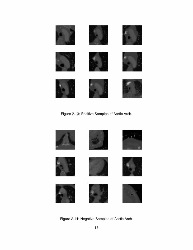
Figure 2.13: Positive Samples of Aortic Arch.

Figure 2.14: Negative Samples of Aortic Arch.

16

AdaBoost without Cascade

For comparison, 100 positive and 500 negative samples were chosen from each

CTPA dataset to train a single AdaBoost. No extra training samples are injected

during the training of 100 weak learners. 100% performance can be achieved on

the training samples, while only 88.75% detection rate in the training cases and

77.92% in the testing are observed, as shown in.

Viola’s AdaBoost Cascading Scheme

For the parameters of Viola’s Cascading Scheme, we started off with 100 positive

and 100 negative samples from each training case. By negative samples injection

between layers, the total number of samples are comparable with the the number

of samples in the previous experiment. The training of a cascade layer is

terminated when αi is over 0.99 and βi is below 0.05 or ηi hits 30. After exiting

from one cascade, the program scans the whole CTPA dataset to select at most

100 false positives from each case as the negative samples for the next layer. The

number of weak learners from cascade 1 to 6 is 1, 9, 22, 30, 30 and 8. In Fig. 2.15,

the accuracy drops and FPR soars when new negative samples are injected. The

FPR increases more dramatically in later cascade as the negative samples in that

cascade are more similar to the positive and hard to be classified correctly. The

accuracy in the detection of the testing cases hits 98.70%, shown in Table 2.1.

Multi-exit AdaBoost Cascading Scheme

We use the same parameters αi, βi, ηi as the previous method. The number of

weak learners for layer 1 to 7 is 1, 9, 23, 40, 62, 90 and 100, respectively. Fig. 2.16

is the performance trend of multi-exit AdaBoost with cascade. The accuracy in the

testing cases reaches 100

17

0 10 20 30 40 50 60 70 80 90 1000

0.1

0.2

0.3

0.4

0.5

0.6

0.7

0.8

0.9

1

TPFPAccuracy

Figure 2.15: The performance of Viola’s AdaBoost cascading scheme in trainingphrase. Layer 1 (weak learner 1); Layer 2 (weak learner 2 - 10); Layer 3 (weaklearner 11 - 32); Layer 4 (weak learner 33 - 62); Layer 5 (weak learner 63 - 92);Layer 6 (weak learner 93 - 100).

0 10 20 30 40 50 60 70 80 90 1000

0.1

0.2

0.3

0.4

0.5

0.6

0.7

0.8

0.9

1

TPFPAccuracy

Figure 2.16: The performance of multi-exit AdaBoost cascading scheming in train-ing phrase. Layer 1 (weak learner 1); Layer 2 (weak learner 1 - 10); Layer 3 (weaklearner 1 - 23); Layer 4 (weak learner 1 - 40); Layer 5 (weak learner 1 - 62); Layer6 (weak learner 1 - 90); Layer 7 (weak learner 1 - 100).

18

AdaBoost with More Representative Negative Samples

To verify the representativeness of the samples and their influence on AdaBoost

algorithm, we inject false positive samples collected from the Viola’s cascading

scheme and multi-exit cascading scheme. The negative sample dataset comsists

of all the negative samples injected between cascading layers. The AdaBoost has

no cascading scheme but contains more representative negative samples. The

accuracy of the detection, shown in Table 2.1, increases significantly from the

orignial AdaBoost without cascading schem. Therefore, the quality of the training

data (i.e. representativeness of the negative training examples) is one of the

utmost important factor for achieving accurate detection.

Table 2.1: Comparison between AdaBoost without cascading, Viola’s cascadingscheme, Multi-exit cascading scheme and AdaBoost with more representative neg-ative samples.

Methods Train Test

AdaBoost without cascading 71/80 (88.75%) 60/77 (77.92%)AdaBoost with more representativenegative samples

77/80 (96.25%) 74/77 (94.10%)

Viola’s cascading scheme [8] 80/80 (100%) 76/77 (98.70%)Multi-exit cascading scheme 79/80 (98.75%) 77/77 (100%)

2.5 Discussion

Besides standard AdaBoost [7, 9] using in Viola’s pioneer work [8], other

researchers advocated the use of RealBoost [15, 16, 17, 18] and GentleBoost

[20]. The concept of AdaBoost, RealBoost and GentleBoost are similar. The key is

to select the best weak learner which can separates the positive from the negative.

And put more weights on misclassified samples so that the next weak learner will

put more emphasis on these samples. However, AdaBoost, RealBoost and

GentleBoost apply different algorithms in selecting the best weak learner and

updating sample’s importance weight.

19

Table 2.2: Pseudo Code of AdaBoost, RealBoost and GentleBoost

Notation:

I(true) = 1, I(false) = 0

αj is the confidence value when h(x) ∈ uj , where∑

j

uj = R

Input:

Training example (xi, yi); yi ∈ {+1,−1} for positive and negative examples respectively.P and N represent the number of positive and negative examples.

Weight Initialization:

w1,i =12P, 12N

for yi = +1.− 1 respectively.

for t = 1, ... , T

1. Normalize examples’ weightwt,i =

wt,i∑

i

wt,i

2. Select the best feature ht(x) and its optimal threshold from the feature pool,based on the error rate.

W+j =

∑

i

I(h(xi) ∈ uj)I(yi = 1)wi

W−j =

∑

i

I(h(xi) ∈ uj)I(yi = −1)wi

2.1 AdaBoost

ǫ =∑

j

min(W+j ,W

−j )

2.2 RealBoost

ǫ =∑

j

√

W+j ·W−

j

2.3 GentleBoost

ǫ =∑

j

2 ·W+

j W−j

W+j +W−

j

3. Calculate the confident value3.1 AdaBoost

αt,j =12· sign(W+

j −W−j ) · ln1−ǫ

ǫ

3.2 RealBoost

αt,j =12· lnW+

j

W−

j

3.3 GentleBoost

αt,j =W+

j −W−

j

W+

j +W−

j

4. Update examples’ weightwt+1,i = wt,i · exp(−|yi| · αt,j)

The final strong classifier is: H(x) = sign(∑T

t=1 αt,j)

20

Table 2.2 combines AdaBoost, RealBoost and GentleBoost into one

pseudocode. The input of the boosting method is the training samples with their

labels. After assigned the weights, the total weights of the positive samples should

be as same as the weights of the negative samples. The training process is in the

loop, in which T is the number of weak learners. Each loop trains one weak

learner. Step 1 normalizes the samples’ weights.

Step 2 picks up the best feature from the feature pool. The feature domain

is separated into several sections. In section j, W+j and W−

j are the total weight of

the positive and negative samples. AdaBoost applies Equation 2.5 to computer ǫ

and selects the feature with smallest ǫ.

ǫ =∑

j

min(W+j ,W

−j ) (2.5)

RealBoost uses Equation 2.6. Supposed the feature distribution of positive

and negative samples are Gaussian, the overlap of the positive and negative

samples should be very small on the feature with lowest ǫ.

ǫ =∑

j

√

W+j ·W−

j (2.6)

GentleBoost is another variant algorithm which utilizes Equation 2.7 as ǫ.

ǫ =∑

j

2 ·W+

j W−j

W+j +W−

j

(2.7)

Fig. 2.17 compares the relationship between positive weight rates and

partition error in AdaBoost, RealBoost and GentleBoost. Positive weight rates are

calculated asW+

j

W+

j +W−

j

. Partition error is the ǫ value under the relative positive

weight rates. If the positive and negative weights are same in a section j, positive

weight rates is 0.5 and the partition error should be high. On the other hand, if

21

positive samples dominate the section or have no appearance in the section, the

partition error should be closed to zero. All of the three methods follow the above

criterion. However, AdaBoost is a linear function. RealBoost and Gentle Boost are

smoother when positive weight rates approaches 0.5.

Figure 2.17: Comparison of error computation among AdaBoost, RealBoost andGentleBoost

Step 3 is the other difference in computing the confidence weight among

AdaBoost, RealBoost and GentleBoost. The absolute value of confidence should

be high when the selected weak learner has low error. The signs of the confidence

value indicate weather the sction is classified as the positive or negative.

AdaBoost, RealBoost and GentleBoost are applying Equation 2.8, 2.9, 2.10

separately for computing confidence value. Fig. 2.18 analysizes the relationship

between positive weight rates and confidence value. AdaBoost and RealBoost

share the same curve. However, in AdaBoost, the confidence value is computed

on the error rate of the all the sections; in RealBoost, the confidence value is

22

based on one section. Thus, the absolute value of AdaBoost is same for all the

section but the sign is different. In RealBoost, different sections can get different

confidence value. GentleBoost is a linear function in the computation of

confidence value. Another nice property of AdaBoost and RealBoost is that they

can reach very high confidence value when the positive weight rate is approaching

0 or 1, but GentleBoost can not.

Figure 2.18: Comparison of confidence value computation among AdaBoost, Real-Boost and GentleBoost

αj =1

2· sign(W+

j −W−j ) · ln1− ǫ

ǫ(2.8)

αj =1

2· ln

W+j

W−j

(2.9)

αj =W+

j −W−j

W+j +W−

j

(2.10)

In step 4, algorithms update training samples’ weights to emphasize on the

misclassified samples. The weight of correctly classified samples is reduced and23

incorrectly classified samples is increased. The next weak learner thus pay more

attention on the misclassified samples to reduce the error rate.

After obtaining T weak learners, the algorithem applies Equation 2.11 to

combine all the weak learner into a strong classifier. The sign of the strong

classifier indicates the classified results. + is positive samples and − is negative

samples.

H(x) = sign(T∑

t=1

αt,j) (2.11)

There are different opinions on the performance of boosting methods.

Lienhart [19] regards RealBoost as the best approach. Brubaker’s result [20]

demonstrates GentleBoost is superior to other approaches. In the thesis, we adopt

AdaBoost for a fair comparison with other methods. Fig. 2.19 illustrates the

training process of AdaBoost. In the images, the radius of the samples are

responsed to their weight. Large radius means bigger weight and vice versa. The

illstration contains two features, representing x axis and y axis respectively. In

Fig. 2.19(a), all the positive samples share the same weight and it’s same to the

negative. In Fig. 2.19(b)-(f), the red dash line is the threshold of the weak learner.

"Red" and "Blue" texts beside the threshold indicates the classification results. If

the classification is wrong, such as the red samples in the left section of

Fig. 2.19(b),the samples becomes larger, which means more weights on this

sample. Therefore, the next weak learner, shown in Fig. 2.19(c), tries to classified

it correctly.

24

Figure 2.19: Demonstration of AdaBoost: (a) Original samples. (b)-(f) Samplesafter reweight based on weak learner 1-5. The radius of the samples are related totheir weight. The red dash line is the threshold of the weak learner. One side of thethreshold is classified as the red and the other is the blue.

25

Chapter 3

ON-LINE ADABOOST

Boosting was originally designed for off-line learning. All training samples have to

be available prior to the training process. The trained classifier cannot be

dynamically adjusted with new coming samples unless retraining from the

beginning, which is time consuming and demands to store all the historical

samples.

In many applications, particularly in medical image analysis, this is a major

drawback as medical data are not generated at one time and retraining is very time

consuming with the increasing number of the training samples. To overcome these

problems, Oza [28] proposed an on-line boosting method, which could update

strong learners without the need for storage of samples and retraining the whole

classifier. Grabner and Bischof [6] improved Oza [28]’s work with a selector-based

structure, achieving impressive performance in object detection and tracking.

Inspired by the work of Grabner and Bischof [6], we propose a novel on-line

learning approach with new weak learner and learning process. The approach

eliminates the need of storing historical training samples, and is capable of

continuously enhancing its performance with new samples. However, our

approach is significantly different from [6] in both the weaker-learner selector and

the learning structure. Because of these two novel contributions, our approach

outperforms [6] in detecting the three distinct anatomic structures, even achieving

a performance comparable to the off-line approaches. Although the performance

are compared on three anatomic structures, our approach is generally applicable

to a variety of anatomical structures.

26

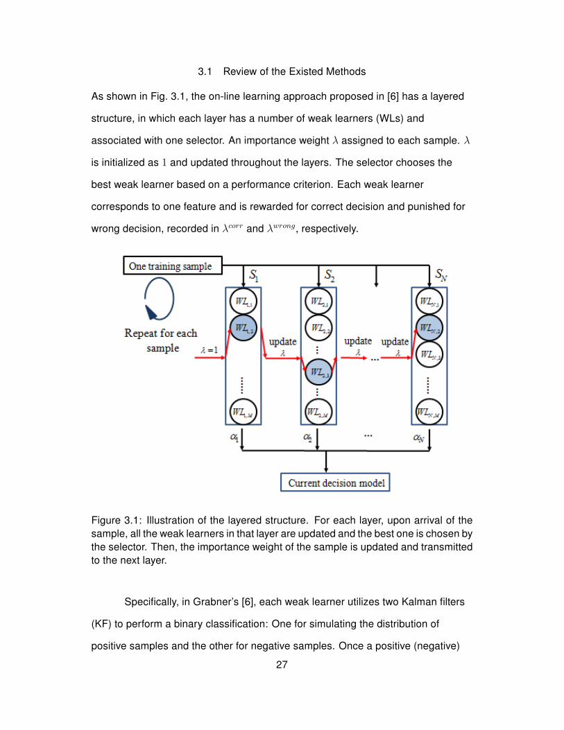
3.1 Review of the Existed Methods

As shown in Fig. 3.1, the on-line learning approach proposed in [6] has a layered

structure, in which each layer has a number of weak learners (WLs) and

associated with one selector. An importance weight λ assigned to each sample. λ

is initialized as 1 and updated throughout the layers. The selector chooses the

best weak learner based on a performance criterion. Each weak learner

corresponds to one feature and is rewarded for correct decision and punished for

wrong decision, recorded in λcorr and λwrong, respectively.

Figure 3.1: Illustration of the layered structure. For each layer, upon arrival of thesample, all the weak learners in that layer are updated and the best one is chosen bythe selector. Then, the importance weight of the sample is updated and transmittedto the next layer.

Specifically, in Grabner’s [6], each weak learner utilizes two Kalman filters

(KF) to perform a binary classification: One for simulating the distribution of

positive samples and the other for negative samples. Once a positive (negative)

27

sample xt arrives at a layer WLi, the KF associated with the positive (negative)

distribution is updated and the threshold θi is determined as follows:

Kt =Pt−1

Pt−1 +R(3.1)

µt = Kt · fi(x) + (1−Kt) · µt−1 (3.2)

Pt = (1−Kt) · Pt−1 (3.3)

θi =µ+t + µ−

t

2(3.4)

where P0, R, and µ are initialized by user, µ+t and µ−

t are the means of the

positive and negative distributions, respectively.

If a weak learner manages to classify the sample into the right category, it

will be rewarded. Otherwise, punishment will be assigned. The reward and

punishment a WL receives are recorded by µcorr and µwrong. Equation 3.5 - 3.7

shows how λ can serve as reward or punishment and how it influences ǫ: the error

of a weak leaner:

Kt =Pt−1

Pt−1 +R(3.5)

µt = Kt · fi(x) + (1−Kt) · µt−1 (3.6)

Pt = (1−Kt) · Pt−1 (3.7)

That is, when a weak learner makes a wrong classification, it is punished

by increasing λwrong. If the classification is correct, it is rewarded by increasing

λcorr. Following the same process for each weak learner, selector can obtain the

accuracy of all the weak learners and picks up the one with least error rate. Then

the voting weight α associated with the best weak learner is computed by the

following formula:

28

α =1

2log

1− ǫ

ǫ(3.8)

The sample’s importance weight λ is also updated and the sample is fed to

the next layer. Equation 3.9 provides the updating rule.

λ =

λ · 12·(1−ǫ)

, if p(x) = y

λ · 12·ǫ, if p(x) 6= y

(3.9)

Interpreted from Equation 3.9, the importance weight λ decreases when

the selector classifies the sample correctly. Otherwise, wrong classification

assigns more weights on the misclassified samples in the next layer.

Following this strategy in each layer, selector can obtain the best weak

learner and its related voting weight. The final decision model is a linear

aggregation of the best weak learners and its voting weight in all the layers.

Assume that the model consists of N layers, the strong classifier D is defined as

follows:

D = sign(∑

(

i = 1)Nαi · di) (3.10)

where di is the decision returned by the best weak learner at ith layer and takes 1

if the sample contains the desired object otherwise -1. di is calculated using the

following formula:

di = sign([fi − θi] · [µ+ − µ−]) (3.11)

3.2 Proposed method: Pool Based On-line AdaBoost

The proposed approach is an on-line feature selection method. Given a set of

training sample, it dynamically updates a pool containing M features and returns a

subset of N best features (N < M ).

29

To our knowledge, we are the first to address anatomical structure

detection with on-line approaches. Other existing approaches are all off-line (e.g.,

[21, 22, 23, 24, 25]) with focus on detection of other major organs like heart, liver,

and spleen.

Figure 3.2: Illustration of the proposed pool structure. Four steps are involved inthe numeric order. Firstly, punish or reward the entire weak learners in the featurepool. Secondly, choose the best feature from the feature pool as the weak learner.Thirdly, compute the weak learner’s voting weight. Finally, update the sample’simportance weight and feed it to choose the next weak learner.

Histogram Weak Learner

For each feature in the pool, the corresponded weak learner is comprised of two

histograms instead of two Kalman filters, one for positive samples and one for

negatives. The two histograms are built as samples come sequentially. In order to

continually update the histograms, the range of each feature in the pool must be

known in advance. The range of the feature is estimated by examining feature30

values computed from a temporary set of samples. The approximated ranges are

equally divided into 100 bins. Note that, it is likely to encounter training samples

whose feature values fall out of the obtained ranges, in that case, they are

assigned to the first or last bin depending on weather they are above the maximum

or below the minimum. The sample updates all the weak learner’s histogram with

its sample weight. And then a threshold for each weak learner is chosen to

minimize the error.

Learning Process

Table 3.1 is the pseudo code of the proposed on-line AdaBoost. When a sample

arrives, all weak learners are updated so as to classify the sample into the right

category.

In step one, if a weak learner manages to classify the sample, it will be

rewarded by the sample’s importance weight λ. λ is high for difficult training

samples and low for easy one. If the samples have not been trained, all weak

learners are rewarded or punished by λ = 1. The reward and punishment are

recorded by λcorr and λwrong which are further used to calculate the error rate of

each weak learner. Having obtained the error rate of all WLs, selector can choose

the best weak learner producing the least error rate.

In step two, the index of selected weak learner is recorded in set A whose

members are not considered when choosing the next best weak learner. This

prevents the duplicated weak learner in the training process.

In step three, selector computes the voting weight αn = 12ln(1−errorm∗

errorm∗)

which indicated the contribution of the weak learner to the final classifier.

In step four, the sample’s importance weight is updated. The change of λ

reflects the power of the selected best weak learner. If the weak learner has

already classified many samples correctly and fails to classify this sample, λ is

31

Table 3.1: Pseudo code of the proposed on-line learning approach

Note: the process is performed for each new sample arriving to the systemRequire: training example (x, y), y ∈ {−1,+1}Require: A feature pool containing M featuresRequire: Total number of weak leaner to be selected N (N < M )Initialization:

Initialize weak learner: λcorrm =1 and λwrongm =1

Initialize set of selected weak learner: A = []Output:

Strong classifier: D(x) = sign(∑N

i=1 αi ·WL∗i (x))

Update all weak learners

Initialize the importance weight λ=1for m = 1,2...,M

WLm=Update(λ,WLm)end

Selecting the best N weak learners

for n = 1,2...,NStep 1: Reward and Punish all M weak learners

for m = 1,2...,Mif WLm(x)=y

λcorrm =λcorrm +λ //correct classificationelse

λwrongm =λwrong

m +λ //wrong classificationenderrorm= λ

wrongm

λcorrm +λ

wrongm

endStep 2: Select the nth best weak learner

m∗=arg min{m 6∈A} errormAdd m∗ to set A

Step 3: Calculate the voting weight of the nth best weak learner

αn = 12ln(1−errorm∗

errorm∗)

Step 4: Update λ, necessary to choose the next best weak learner

if WL∗m(x)=y

λ= λ2(1−errorm∗ )

//correct decision

elseλ= λ

2(errorm∗ )//wrong decision

endend

32

increased dramatically. On the other hand, if the weak learner is known to perform

a poor accuracy, it cannot significantly increase λ. The rational behind using and

updating λ is to stimulate the next best weak learner to correct the misclassified

samples from previous best weak learners.

The output is a strong classifier D(x) = sign(∑N

i=1 αi ·WL∗i (x)). If the

result is 1, the sample is classified as positive. −1 is the negative samples.

3.3 Experiment and Result

The experiment exploits 157 CT pulmonary angiogram datasets, of which 80

datasets are used for training the decision model and the rest are for testing. Each

dataset contains 450 ∼ 600 slices. To construct the training samples, 80 training

patients are scanned and positive and negative samples of 25x25 pixels are

extracted. Because of simplicity and efficiency, Haar features [8] are computed for

each 25x25 training sample. Using two Haar patterns of different positions, scales,

and aspect ratio, we obtain 101,400 features for each training sample.

Table 3.2 summarizes the detection rates obtained from both off-line and

on-line detectors for the training and test patients. the results derived from For our

method, we include results deriving from (1) only the novel learning structure as

"Proposed + KF" and (2) both the novel learning structure and better weak learner

representation as "Proposed + Histogram".

Table 3.2: The detection rates on the pulmonary trunk, the aortic arch and thecarina. (Proposed + KF)I and(Proposed + Histogram) stand for proposed learningstructure using Kalman Filter and Histogram as weak learner, respectively.)

Methods PT[%] Carina[%] Aortic Arch[%]Train Test Train Test Train Test

Grabner and Bischof [6] 87.5 79.2 98.7 93.4 36.3 47.4Proposed + Kalman Filter 86.2 88.3 96.2 97.4 63.4 69.7Proposed + Histogram 95.0 89.6 97.5 98.7 73.8 77.6Off-line AdaBoost [8] 97.5 93.5 100 100 95.0 93.4

33

Comparison with Grabner and Bischof [6]: In the case of carina, the

proposed method using either Kalman filter or histograms slightly outperforms the

Grabner’s approach. The small variation in scale and orientation accounts for the

high carina detection rates. However, the situation for the pulmonary trunk and

aortic arch is quite different. Table 3.2 shows a remarkable drop in the detection

rates of both on-line approaches though the proposed method achieves higher

performance. Outliers and the wide range of variation in object’s scale and

orientation decrease the performance and they will be further discussed in the

next section.

Comparing to Grabner’s approach[6], the performance of the proposed

method with pool learner process achieve better performance, explaining the

superiority of the proposed learning structure.

3.4 Discussion

This section will further discuss the stability, regarding to outlier. And we will also

compare the efficiency and accuracy of Kalman filter and histogram.

Stability

A non-rigid anatomic structure is attributed to human body structures appearing

with variation in shape, scale, and orientation from patient to patient. Fig. 3.3

shows four samples for each desired anatomic structures. For each structure, the

first two samples stand for the typical shape of the structure while the other

samples include notable variation in orientation and shape. As it is seen, while the

carina samples exhibit higher level of rigidity, the aortic arch and pulmonary trunk

samples display lower rigidity. In this study, the samples which markedly differ in

appearance from the typical shape of the structures are referred as positive

outliers. Positive outliers affect the learning process and deteriorate the accuracy

of the strong weak learner.

34

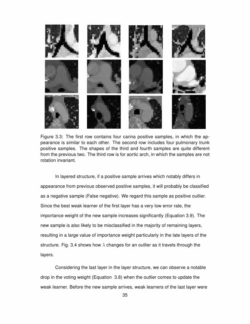
Figure 3.3: The first row contains four carina positive samples, in which the ap-pearance is similar to each other. The second row includes four pulmonary trunkpositive samples. The shapes of the third and fourth samples are quite differentfrom the previous two. The third row is for aortic arch, in which the samples are notrotation invariant.

In layered structure, if a positive sample arrives which notably differs in

appearance from previous observed positive samples, it will probably be classified

as a negative sample (False negative). We regard this sample as positive outlier.

Since the best weak learner of the first layer has a very low error rate, the

importance weight of the new sample increases significantly (Equation 3.9). The

new sample is also likely to be misclassified in the majority of remaining layers,

resulting in a large value of importance weight particularly in the late layers of the

structure. Fig. 3.4 shows how λ changes for an outlier as it travels through the

layers.

Considering the last layer in the layer structure, we can observe a notable

drop in the voting weight (Equation 3.8) when the outlier comes to update the

weak learner. Before the new sample arrives, weak learners of the last layer were

35

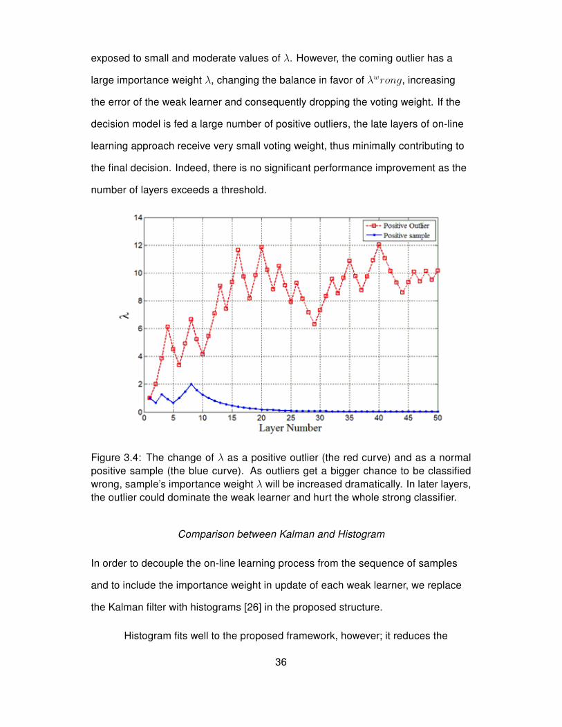
exposed to small and moderate values of λ. However, the coming outlier has a

large importance weight λ, changing the balance in favor of λwrong, increasing

the error of the weak learner and consequently dropping the voting weight. If the

decision model is fed a large number of positive outliers, the late layers of on-line

learning approach receive very small voting weight, thus minimally contributing to

the final decision. Indeed, there is no significant performance improvement as the

number of layers exceeds a threshold.

Figure 3.4: The change of λ as a positive outlier (the red curve) and as a normalpositive sample (the blue curve). As outliers get a bigger chance to be classifiedwrong, sample’s importance weight λ will be increased dramatically. In later layers,the outlier could dominate the weak learner and hurt the whole strong classifier.

Comparison between Kalman and Histogram

In order to decouple the on-line learning process from the sequence of samples

and to include the importance weight in update of each weak learner, we replace

the Kalman filter with histograms [26] in the proposed structure.

Histogram fits well to the proposed framework, however; it reduces the

36

efficiency of the original approach. The rationale behind assigning the same

subset of WLs to each layer is to update all WLs once when a new sample arrives.

It can be realized when we update the decision threshold of each WL irrespective

of the importance weight. However, the histogram-based weak learner requires

M ·N ·NumberOfBins operations when updating all the features, increasing the

computational time and reducing memory efficiency. NumberOfBins usually is

set as 200. On the other side, Kalman filter requires M ·N · 2 operations.

37

Chapter 4

ON-LINE ASYMMETRIC ADABOOST

4.1 Review of the Existed Methods

Grabner and Bischof’s method [6] is popular in on-line learneing. However, in their

implementation, they strictly picked up one positive and four negative samples in

each frame and then duplicated positive samples four times to equalize the

number of positive and negative samples. In medical image process, the

assumption of same number of positive and negative samples is unrealistic. For

instance, in each CT pulmonary angiography, there is only one carina, one

pulmonary trunk and one aortic arch, which play significant roles in designing a

computer-aided diagnosis for detecting pulmonary embolism—one of the most

lethal and difficult diagnostic conditions in medicine. As there are far more

negative samples than positive in medical image dataset and we do not know the

distribution of positive and negative samples, the balanced assumption is not

reasonable.

To deal with the imbalanced samples, asymmetric learning was first

introduced by Viola and Jones [29]. They developed an asymmetric loss criterion

associated with a preset parameter k to penalize k times more on false negative

than on false positive. The loss criterion was also adopted in [31]. Pham, et al.

[30] utilized two preset parameters, maximum false acceptance rate α0 and

maximum false rejection rate β0, to setup the asymmetric loss criterion. Pham, et

al.’s paper [31] switched their preset parameter to k, which was used in [29]. The

existing asymmetric methods require preset parameters; they are not capable of

adjusting the asymmetric loss criterion during the training process. There is no

general rule for selecting these preset parameters and they have to be chosen

based on experience. Different applications may require different parameters.

In medical image analysis, it is not possible to pre-determine the

38

parameters about the skewness of samples. For instance, in the context of

anatomical structure detection, we may generate hundreds of distinguished

positive samples around the structure of interest (see Fig. 1.3), but there are

countless negative samples all over the dataset. Thus, we propose a self-adaptive,

asymmetric on-line boosting (SAAOB) method for detecting anatomical structures

in CT pulmonary angiography. SAAOB is novel in that it exploits a new asymmetric

loss criterion with self-adaptability according to the ratio of exposed positive and

negative samples and in that it has an advanced rule to update sample’s

importance weight taking account of both classification result and sample’s label.

Validation and comparison are presented based on the experiments to detect the

carina, the pulmonary trunk and the aortic arch in both balanced and imbalanced

conditions.

The remaining of the chapter is organized as follows. Section 4.2

introduces the methodology and structure of SAAOB, while Section 4.3 presents

its performance in both balanced and imbalanced conditions, followed by a

discussion in Section 4.4.

4.2 Self-Adaptive Asymmetric On-line Boosting (SAAOB)

SAAOB is an asymmetric version derived from Grabner and Bischof’s on-line

boosting [6] in which selectors share the same feature pool. This section

discusses the contribution, the loss criterion and sample’s weight updating rules

with the pseudo code of SAAOB (Table 4.1).

Contribution

As the first contribution, we introduce a new asymmetric loss criterion with self

adaptability according to the ratio of exposed positive and negative samples.

Symmetric on-line learning methods [28, 6] simply update sample’s importance

weight according to the classification result. In asymmetric on-line learning, it is

39

compelling to update sample’s importance weight differently in the situations of

true positive, false positive, true negative and false negative.

As our second contribution, SAAOB applies an advanced set of formulas in

the four aforementioned situations. As an asymmetric on-line method, SAAOB

needs to have different formulas for positive and negative samples. We introduce

a set of four different formulas for updating sample’s importance weight when the

classification is true positive, false positive, true negative and false negative.

The third contribution is the application of SAAOB in the automated

detection of anatomical structures. We focus on three anatomical structures,

namely, the carina, the pulmonary trunk and the aortic arch (Fig. 1.3) because

they provide initial regions of interest for segmentation, and landmarks for

registration and navigation. They are particularly important for our current project,

requiring extraction of pulmonary artery and airway.

We validate SAAOB from the balanced condition (1 positive: 1 negative) to

the extremely imbalanced condition (1 positive: 1000 negative), showing that

SAAOB outperforms Grabner and Bischof [6]’s work in imbalanced conditions with

slightly better performance in balanced condition.

Asymmetric Loss Criterion

The limitation of on-line boosting methods with symmetric loss criterion [28, 6]

arises in the imbalanced conditions in which the number of negative samples is far

more than that of positive samples. For example, in the application of detecting

anatomical structure, there are at most hundreds of the positive images of the

desired structure among millions of the negative images in one patient dataset.

The symmetric loss criterion:

E =λFN

λTP + λFP + λTN + λFN+

λFP

λTP + λFP + λTN + λFN(4.1)

40

Table 4.1: Pseudo code of the proposed method: SAAOB

Note: the process is performed for each new sample arriving to the systemRequire: training example (x, y), y ∈ {−1,+1}Require: weights λTP

n,m, λFPn,m, λTN

n,m, λFNn,m (initialized with 1)

Require: sample’s importance weight λ (initialized with 1)Require: posnum and negnum are the numbers

of positive and negative samples been exposed to SAAOB (initialized with 1)

for m = 1,2,...,M do // update all the weak learnershweakm = update( hweak

m ,(x,y))end for

for n = 1,2,...,N do // update the weak learner parameters in all selectorsfor m = 1,2,...,M do // update the weak learner parameters in selector n

// estimate errorsif hweak

n,m (x) = +1 and y = +1 then // true positiveλTPn,m = λTP

n,m + λelse if hweak

n,m (x) = +1 and y = −1 then // false positiveλFPn,m = λFP

n,m + λelse if hweak

n,m (x) = −1 and y = −1 then // true negativeλTNn,m = λTN

n,m + λelse if hweak

n,m (x) = −1 and y = +1 then // false negativeλFNn,m = λFN

n,m + λend if

// asymmetric loss criterion

En,m = 11+2ǫ

[( negnum

posnum+negnum + ǫ)λFNn,m

λTPn,m+λFP

n,m+λTNn,m+λFN

n,m

+( posnum

posnum+negnum + ǫ)λFPn,m

λTPn,m+λFP

n,m+λTNn,m+λFN

n,m]

end for

// choose the best weak learner and get the parameters for selector nmbest = argminm(en,m);h

seln = hweak

n,mbest ; En = En,mbest;αn = log 1−en

en

λTPn = λTP

n,mbest;λFP

n = λFPn,mbest

;λTNn = λTN

n,mbest;λFN

n = λFNn,mbest

//update sample’s importance weightif hseln (x) = +1 and y = +1 then // true positive

λ = 12λ posnum+negnum

λTPn +λFP

n +λTNn +λFN

n

λTPn +λFP

n

λTPn

else if hseln (x) = +1 and y = −1 then // false positive

λ = 12λ posnum+negnum

λTPn +λFP

n +λTNn +λFN

n

λTPn +λFP

n

λFPn

else if hseln (x) = −1 and y = −1 then // true negative

λ = 12λ posnum+negnum

λTPn +λFP

n +λTNn +λFN

n

λTNn +λFN

n

λTNn

else if hseln (x) = −1 and y = +1 then // false negative

λ = 12λ posnum+negnum

λTPn +λFP

n +λTNn +λFN

n

λTNn +λFN

n

λFNn

end if

end for

hstrong(x) = sign(∑N

n=1 αnhseln (x)) // strong learner

41

equally emphasizes on false negative rate and false positive rate to choose the

best weak learner. λTP , λFP , λTN , λFN respectively refer to the true positive, false

positive, true negative and false positive weights of a weak learner.

Viola and Jones [29] developed an asymmetric loss criterion for off-line

AdaBoost:

E =√k

λFN

λTP + λFP + λTN + λFN+

√

1

k

λFP

λTP + λFP + λTN + λFN(4.2)

to penalize false negative k times more than false positive. k needs to be known in

advance and cannot change during the training. The selection of k is based on

designers’ experience rather than the skewness of the samples.

We introduce a new asymmetric loss function which can adjust itself during

the on-line training:

E =1

1 + 2ǫ[(

negnum

posnum + negnum+ ǫ)

λFN

λTP + λFP + λTN + λFN

+(posnum

posnum + negnum+ ǫ)

λFP

λTP + λFP + λTN + λFN]

(4.3)

where posnum and negnum are the numbers of positive and negative samples

which have been exposed to SAAOB, and ǫ is a smoothing factor. In extremely

imbalanced conditions, where negnum

posnum+negnum → 1 and posnum

posnum+negnum → 0, the cost

of false negative is 1+ǫǫ

times more than the cost of false positive. In balanced

condition, when posnum ≈ negnum, the weights of false negative error and false

positive error are same. Naturally, SAAOB outperforms Grabner[6] in imbalanced

conditions and should work equally well in balanced condition.

Sample’s Importance Weight

Grabner and Bischof [6] updated sample’s importance weight with

φ =

11−E

, if p(x) = y

1E, if p(x) 6= y

(4.4)

42

λ =1

2λφ (4.5)

where x is the sample and y is the label of x. p(x) is the prediction by the

classification. This means that their updating rules only depend on the

classification result rather than on the sample’s label. In asymmetric on-line

learning, positive and negative samples must be treated differently. Therefore, it

demands different rules for true positive, false positive, true negative, false

negative. Considering skewness of samples, classification result and sample’s

label, we have

ϕ =posnum + negnum

λTPn,m + λFP

n,m + λTNn,m + λFN

n,m

(4.6)

ψ =

λTP+λFP

λTP , if p(x) = +1 and y = +1 // true positive

λTP+λFP

λFP , if p(x) = −1 and y = +1 // false positive

λTN+λFN

λTN , if p(x) = −1 and y = −1 // true negative

λTN+λFN

λFN , if p(x) = +1 and y = −1 // false positive

(4.7)

λ =1

2λϕψ (4.8)

yielding more accurate sample’s weight updating in SAAOB.

4.3 Experiments and resultsDatasets

The experiments involve in 157 CT pulmonary angiograms datasets, in which 80

datasets are used for training and the rest are for testing. Each dataset contains

450 - 600 512-by-512-pixels slices with 0.5mm×0.5mm to 0.7mm×0.7mm pixel

size. The thickness between slices is 0.5 mm. We adopt Wu, et al.’s prototype [27]

to generate 4000 positive and 16000 negative 25-by-25-pixels training images

from the 80 training datasets for the carina, the pulmonary trunk and the aortic

arch separately.

43

Training Process

Two types of Haar feature patterns [8], horizontal one and vertical one, have been

adopted in our experiments, resulting in 101400 Haar features. In the experiments,

we uses 50 selectors which share one feature pool with 100 Haar features. The

smoothing factor ǫ used in asymmetric loss criterion is set to 0.25. According to

equation (4.3), in extreme case, where negative ≫ positive, SAAOB at most

penalizes 5 times more on false negative than on false positive.

The ratio of positive and negative samples ranges from 1:1 (balanced

condition) to 1:1000 (extremely imbalanced condition). We use all 16000 negative

samples in the experiment. If the need of positive samples is less than 4000, we

randomly select positive samples from the 4000. If the need is more than 4000, we

duplicate the positive samples.

Testing Process and Performance Criterion

Detection is based on Viola-Jones’ seminal work in face detection [8]. Two levels

of testing, sample level and patient level, are conducted in the experiments. At

sample level, the trained strong learners are tested on another 25-by-25-pixels

image set which also contains 4000 positive samples and 16000 negative samples

but all of them are different from the training images. The performance is

evaluated by their ROC curves and ROC’s AUC (area under curve). At patient

level, we applied the strong learners to detect the anatomical structures in 77

testing datasets. If the distance between detection point and ground truth is less

than 15 mm, the detection is regarded as correct.

Comparison

Fig. 4.1, Fig. 4.2 and Table 4.2 are the experiment results at sample level.

Because of the space limitation, we only include the comparison in aortic arch

44

Table 4.2: Comparison on AUC between Grabner’s symmetric approach[6] and theproposed SAAOB in detecting the pulmonary trunk, the carina and aortic arch.

Apps Pulmonary TrunkMethods Grabner[6] SAAOB1 :1000 0.9352 0.94391 :500 0.9458 0.96791 :200 0.9513 0.96931 :100 0.9516 0.97351 :50 0.9613 0.97691 :20 0.9716 0.97631 :10 0.9774 0.97911 :5 0.9824 0.98201 :2 0.9863 0.98451 :1 0.9867 0.9871

Apps CarinaMethods Grabner[6] SAAOB1 :1000 0.9963 0.99491 :500 0.9970 0.99531 :200 0.9976 0.99741 :100 0.9982 0.99831 :50 0.9977 0.99881 :20 0.9982 0.99901 :10 0.9989 0.99931 :5 0.9992 0.99921 :2 0.9991 0.99921 :1 0.9995 0.9997

Apps Aortic ArchMethods Grabner[6] SAAOB1 :1000 0.8873† 0.9503†

1 :500 0.9299 0.95021 :200 0.9178 0.96681 :100 0.9226† 0.9689†

1 :50 0.9274 0.97411 :20 0.9415 0.97601 :10 0.9541 0.97891 :5 0.9505 0.98031 :2 0.9697 0.97891 :1 0.9736† 0.9795†

†: Refer to Fig. 4.1 for ROC curves.‡: The data in the column are also shown in Fig. 4.2.

45

0 0.1 0.2 0.3 0.4 0.5 0.6 0.7 0.8 0.9 10

0.1

0.2

0.3

0.4

0.5

0.6

0.7

0.8

0.9

1

1−Speceficity

Sen

sitiv

ity

ROC of Aortic Arch Experiment

1:1, Grabner[6]1:100, Grabner[6]1:1000, Grabner[6]1:1, SAAOB1:100, SAAOB 1:1000, SAAOB

Figure 4.1: The dash-dot lines are the ROC curves by using Grabner[6]. The solidlines are generated by applying SAAOB. From top-left to bottom-right, both ROCcurves are in the conditions (positive: negative) 1:1, 1:100 and 1:1000.

detection. Fig. 4.1 are ROC curves and Fig. 4.2 are the changing trend of AUC in

Table 4.2. In detecting the aortic arch, SAAOS’s performance in harder extreme

condition (1 positive: 100 negative) is much better than Grabner[6]’s performance

in an easier extreme condition (1 positive: 10 negative) and SAAOS’s performance

in (1 positive: 100 negative) even approaches to the performance of Grabner[6] in

the balanced condition, shown in Fig. 4.1. Table 4.2 also demonstrates the major

improvement of SAAOB from Grabner[6] in the pulmonary trunk and the aortic

arch detection. Meanwhile, SAAOB also achieves very good performance in

detecting the carina as Grabner[6].

Patient level result Table 4.3 indicates consistent results as sample level.

SAASO demonstrates much better performance in the imbalanced conditions in

detecting the aortic arch and the pulmonary trunk. Because of the smoothing

46

100

101

102

103

0.85

0.9

0.95

1

Ratio (Negative : Positive)

Are

a U

nder

Cur

ve

AUC of Aortic Arch ROC

Grabner[6]SAAOB

Figure 4.2: The results are from the experiment on the aortic arch. The dash-dotline is the ROC’s AUC by using Grabner[6] and the solid line is from SAAOB. Thepoints represent the performance under the ratio (positive: negative) 1:1, 1:2, 1:5,1:10, 1:20, 1:50, 1:100, 1:200, 1:500 and 1:1000.

factor, SAASO’s performance in the balanced condition is as good as or a little

better than Grabner[6]’s method. Table 4.3 also shows that SAASO has same

good generalization in different applications.

Instead of getting the model by fixing the number of negative samples and

reducing the number of positive samples, we fix the number of positive samples

and increase the number of negative samples to achieve the imbalanced situation.

In Table 4.4, the most imbalanced situation is 1:50 as it may take several months

to get all the data in Table 4.3. By comparing Table 4.3 and Table 4.4, we can see

that SAASO gets better performance than Grabner[6]’s method in both

experiments.

4.4 Discussion

In this Chapter, we propose a new asymmetric loss function with self adaptability

and exploit a set of formulas to update sample’s weight with classification result

47

and sample’s label. Our on-line asymmetric method SAAOB achieves better

performance than Grabner [6] in imbalanced conditions. Meanwhile, no need of

preset parameters guarantees the stable generalization of SAAOB in all the three

anatomical structures detection

The performance of the detection is affected by the hardness of anatomical

structures. As the intensity of the carina is much lower than its surroundings, it

may be easy to detect the carina. Both SAAOB and Grabner[6] can handle the

imbalanced conditions in detecting the carina and achieve good accuracy. Among

the three anatomical structures, the carina and the pulmonary trunk have obvious

bifurcation structures, which may help them to be detected. 2-D Haar feature was

used because of (a) its popularity and efficiency; (b) an unbiased comparison with

Grabner’s method [6]; (c) our focus on developing a novel learning method rather

than designing features. In the future, we will try 3-D Haar features to improve the

performance of the classification.

48

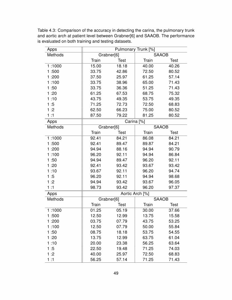
Table 4.3: Comparison of the accuracy in detecting the carina, the pulmonary trunkand aortic arch at patient level between Grabner[6] and SAAOB. The performanceis evaluated on both training and testing datasets.

Apps Pulmonary Trunk [%]Methods Grabner[6] SAAOB

Train Test Train Test1 :1000 15.00 18.18 40.00 40.261 :500 33.75 42.86 72.50 80.521 :200 37.50 25.97 61.25 57.141 :100 33.75 38.96 65.00 71.431 :50 33.75 36.36 51.25 71.431 :20 61.25 67.53 68.75 75.321 :10 43.75 49.35 53.75 49.351 :5 71.25 72.73 72.50 68.831 :2 62.50 66.23 75.00 80.521 :1 87.50 79.22 81.25 80.52

Apps Carina [%]Methods Grabner[6] SAAOB

Train Test Train Test1 :1000 92.41 84.21 86.08 84.211 :500 92.41 89.47 89.87 84.211 :200 94.94 88.16 94.94 90.791 :100 96.20 92.11 94.94 86.841 :50 94.94 89.47 96.20 92.111 :20 92.41 93.42 93.67 93.421 :10 93.67 92.11 96.20 94.741 :5 96.20 92.11 94.94 98.681 :2 94.94 93.42 93.67 96.051 :1 98.73 93.42 96.20 97.37

Apps Aortic Arch [%]Methods Grabner[6] SAAOB

Train Test Train Test1 :1000 01.25 05.19 30.00 37.661 :500 12.50 12.99 13.75 15.581 :200 03.75 07.79 43.75 53.251 :100 12.50 07.79 50.00 55.841 :50 08.75 18.18 53.75 54.551 :20 13.75 12.99 63.75 61.041 :10 20.00 23.38 56.25 63.641 :5 22.50 19.48 71.25 74.031 :2 40.00 25.97 72.50 68.831 :1 56.25 57.14 71.25 71.43

49

Table 4.4: Comparison of the accuracy in detecting the carina, the pulmonary trunkand aortic arch at patient level between Grabner[6] and SAAOB. The performanceis evaluated on both training and testing datasets. The model is calculated byincresing the number of negative samples

Apps Pulmonary Trunk [%]Methods Grabner[6] SAAOB

Train Test Train Test1 :50 15.00 16.88 75.00 79.221 :40 23.75 22.08 50.00 46.751 :30 37.50 41.56 82.50 77.921 :20 45.00 48.05 77.50 77.921 :15 60.00 63.64 77.50 80.521 :10 43.75 54.55 78.75 75.321 :5 33.75 44.16 70.00 67.531 :2 55.00 58.44 76.25 79.221 :1 80.00 84.42 78.75 83.12

Apps Carina [%]Methods Grabner[6] SAAOB

Train Test Train Test1 :50 93.67 92.11 98.73 98.681 :40 86.08 90.79 94.94 97.371 :30 98.73 93.42 98.73 97.371 :20 98.73 97.37 92.41 96.051 :15 91.14 92.11 92.41 94.741 :10 94.94 94.74 97.47 93.421 :5 91.14 94.74 97.47 90.791 :2 94.94 96.05 93.67 97.371 :1 97.47 96.05 97.47 92.11

Apps Aortic Arch [%]Methods Grabner[6] SAAOB

Train Test Train Test1 :50 06.25 20.78 51.25 57.141 :40 12.50 20.78 53.75 42.861 :30 13.75 25.97 45.00 48.051 :20 08.75 24.68 37.50 33.771 :15 11.25 15.58 31.25 48.051 :10 17.50 24.68 67.50 61.041 :5 42.50 42.86 45.00 44.161 :2 31.25 29.87 42.50 44.161 :1 38.75 49.35 56.25 61.04

50

Chapter 5

CONCLUSION

The purpose of the thesis is to detect anatomical structures, including the

pulmonary trunk, the carina and the aortic arch. We explore both offline method

and online method to achieve the goal. In order to improve the performance, we

also deal with the asymmetric learning problems.

In off-line AdaBoost, we review several knowledge based methods and

indicate the major problem of these methods are bad generalization. We develop

an off-line AdaBoost with multi-exit cascading scheme. The proposed method has

been developed to detect the pulmonary trunk, which is opaque to anatomy

knowledge of the underlying interesting subjects. The system is insensitive to the

position, size and intensity variations of the pulmonary trunk and it can achieve

very high accuracy.

The drawbacks of the off-line AdaBoost are presented in Chapter 3. We

improved the original on-line method and proposed a new on-line learning

framework. The new framework were evaluated on three anatomic structures with

different levels of rigidity, demonstrating the proposed method surpasses

Grabner’s method [6] on the pulmonary trunk and the aortic arch with low level of

rigidity. The proposed method also achieves similar performance on the carina

which obtains high rigidity. To our knowledge, the presented work is among the

first attempts to tackle the anatomic structure detection in on-line learning aspect.

We further proposed a novel asymmetric loss function with self adaptability

and exploit a set of formulas to update sample’s weight with classification result

and sample’s label. The proposed online asymmetric method achieved better

performance than Grabner’s method [6] in imbalanced conditions. Meanwhile, no

need of preset parameters guaranteed the stable generalization of SAAOB in all

51

the three anatomical structures detection.

For the future, we plan to

1. extend the 2-D Haar feature into 3-D to capture more distinguishing and

representative features for the anatomical structures.

2. apply the algorithm to more anatomical structures, such as the tips of the

lung, the ribs or the spine.

3. automatically design the cascade scheme rather than tuning manually.

52

REFERENCE

[1] Bouma, H. and Sonnemans ,J.J.: Automatic Detection of Pulmonary Embolism

in CTA Images. In: IEEE Transactions on Medical Imaging, vol. 28, pp.

1223-1230 (2009)

[2] Zhou, C. and Chan, H.: Automatic Multiscale Enhancement and Segmentation

of Pulmonary Vessels in CT Pulmonary Angiography Images for CAD

Applications. In: Medical Physics, vol. 34, pp. 4567-4577 (2007)

[3] Liang, J. and Bi, J.: Computer Aided Detection of Pulmonary Embolism with

Tobogganing and Mutiple Instance Classification in CT Pulmonary

Angiography. In: Information Processing in Medical Imaging, vol. 20, pp.

630-641 (2007)

[4] Dundar, M.M. and Fung, G.: Multiple-instance Learning Algorithms for

Computer-aided Detection. In: IEEE Transactions on Bio-Medical Engineering,

vol. 55, pp. 1015-1021 (2008)

[5] Rathbun, S. :The Surgeon General’s Call to Action to Prevent Deep Vein

Thrombosis and Pulmonary Embolism. In: Circulation, vol. 119, pp. e480-482

(2009)

[6] Grabner, H., Bischof, H.: On-line Boosting and Vision. In: Computer Vision and

Pattern Recognition, IEEE Computer Society Conference on, pp. 260–267

(2006)

[7] Freund, Y. and Schapire, R.E.: A Short Introduction to Boosting. In: the

Sixteenth International Joint Conference on Artificial Intelligence, pp.

1401-1406 (1999)

53

[8] Viola, P. and Jones M.: Rapid object detection using a boosted cascade of

simple features. In: Computer Vision and Pattern Recognition, pp. 511-518

(2001)

[9] Schapire, R.E. and Singer, Y.: BoosTexter: A Boosting-based System for Text

Categorization. In: Machine Learning, 39, pp. 135-168 (2000)

[10] Yow, K.C. and Cipolla, R.: Feature-Based Human Face Detection. In: Image

and Vision Computing, vol. 15, no.9, pp. 713-735 (1997)

[11] Yang, G. and Huang, T.S.: Human Face Detection in Complex Background.

In: Pattern Recognition, vol. 27, no. 1, pp. 53-63 (1994)

[12] Scassellati, B.: Eye Finding via Face Detection for a Foevated, Active Vision

System. In: Proc. of 15th NatŠl Conf. Artificial Intelligence (1998)

[13] Zou X., et al: Anatomy-based Automatic Detection and Segmentation of

Major Vessels in Thoracic CTA Images. In: International Journal of Computer

Assisted Radiology and Surgery, vol. 2, pp. 68-81 (2007)

[14] Crow, F.C.: Summed-area Tables for Texture Mapping. In: SIGGRAPH

Comput. Graph., vol. 18, pp. 207-212 (1984)

[15] Li, S., Zhu, L., Zhang, Z., Blake, A., Zhang, H., and Shum, H.: Statistical

learning of multi-view face detection. In: 7th European Conference on

Computer Vision, pp. 67-81 (2002)

[16] Bishop, C. and Viola, P.: Learning and vision: Discriminative methods. In:

ICCV Course on Learning and Vision (2003)

54

[17] Wu, B. , Ai, H., Huang, C., and Lao, S.: Fast rotation invariant multi-view face

detection based on real adaboost. In: IEEE Automatic Face and Gesture

Recognition, pp. 79-84 (2004)

[18] Mita, T., Kaneko, T., and Hori, O.: Joint Haar-like features for face detection.

In: ICCV IEEE International Conference on , vol. 2, pp. 1619-1626 (2005)

[19] Lienhart, R., Kuranov, A., and Pisarevsky, V.: Empirical analysis of detection

cascades of boosted classifiers for rapid object detection. In: Pattern

Recognition, pp. 297-304. (2003)

[20] Brubaker, S.C., Wu, J., Sun, J., Mullin, M.D., and Rehg, J.M.: On the design

of cascades of boosted ensembles for face detection. Technical report,

Georgia Institute of Technology, GIT-GVU-05-28 (2005)

[21] Zheng, Y., Barbu, A., Georgescu, B., Scheuering, M., and Comaniciu, D.:

Fast Automatic Heart Chamber Segmentation from 3D CT Data Using

Marginal Space Learning and Steerable Features. In: ICCV , 8 pages (2007)

[22] Liu, D., Zhou, K. S., Bernhardt, D., Comaniciu, D.: Search Strategies for

Multiple Landmark Detection by Submodular Maximization. In: CVPR, pp.

2831-2838 (2010)

[23] Zheng, Y., Georgescu, B., Ling, H., Zhou, K. S., Scheuering, M., Comaniciu,

D.: Constrained Marginal Space Learning for Efficient 3D Anatomical Structure

Detection in Medical Images. In: CVPR , pp.194-201 (2009)

[24] Criminisi, A., Shotton, J., Bucciarelli, S.: Decision Forests with Long-Range

Spatial Context for Organ Localization in CT Volumes. In: MICCAI Workshop

55

on Probabilistic Models for Medical Image Analysis (2009)

[25] Criminisi, A., Shotton, J., Robertson, D., Konukoglu, E.: Regression Forests

for Efficient Anatomy Detection and Localization in CT Studies. In

MICCAI-MCV Workshop , pp. 106-117 (2010)

[26] Wu, B., Nevatia, R.: Improving part based object detection by unsupervised,

online boosting. In: International Conference on Computer Vision and Pattern

Recognition, pages 1-8 (2007)

[27] Wu, H., Deng, K., Liang, J.,: Machine Learning based Automatic Detection of

Pulmonary Trunk. In: Medical Imaging, SPIE, Vol.7963. (2011)

[28] Oza N.C., Russell, S.: Online Bagging and Boosting. In: Artificial Intelligence

and Statistics, pp. 105–112 (2001)

[29] Viola, P., Jones, M.: Fast and robust classification using asymmetric

AdaBoost and a detector cascade. In: Advances in Neural Information

Processing System, Vol. 14, pp. 1311-1318 (2002)

[30] Pham, M-T, Hoang, V-D.D, Cham T-J: Detection with multi-exit asymmetric

boosting. In: Computer Vision and Pattern Recognition, pp. 1-8 (2008)

[31] Pham, M-T, Cham T-J: Online Learning Asymmetric Boosted Classifiers for

Object Detection. In: Computer Vision and Pattern Recognition, p. 1 (2007)

56