Accelerating Online Reinforcement Learning withOffline Datasets

Ashvin NairUC Berkeley

Murtaza DalalUC Berkeley

Abhishek GuptaUC Berkeley

Sergey LevineUC Berkeley

Abstract

Reinforcement learning provides an appealing formalism for learning controlpolicies from experience. However, the classic active formulation of reinforcementlearning necessitates a lengthy active exploration process for each behavior, makingit difficult to apply in real-world settings. If we can instead allow reinforcementlearning to effectively use previously collected data to aid the online learningprocess, where the data could be expert demonstrations or more generally anyprior experience, we could make reinforcement learning a substantially morepractical tool. While a number of recent methods have sought to learn offline frompreviously collected data, it remains exceptionally difficult to train a policy withoffline data and improve it further with online reinforcement learning. In this paperwe systematically analyze why this problem is so challenging, and propose a novelalgorithm that combines sample-efficient dynamic programming with maximumlikelihood policy updates, providing a simple and effective framework that is able toleverage large amounts of offline data and then quickly perform online fine-tuningof reinforcement learning policies. We show that our method enables rapid learningof skills with a combination of prior demonstration data and online experienceacross a suite of difficult dexterous manipulation and benchmark tasks.

1 Introduction

Learning models that generalize effectively to complex open-world settings, from image recogni-tion [8] to natural language processing [3], relies on large, high-capacity models and large, diverse,and representative datasets. Leveraging this recipe for reinforcement learning (RL) has the potentialto yield powerful policies for real-world control applications such as robotics. However, whiledeep RL algorithms enable the use of large models, the use of large datasets for real-world RL isconceptually challenging. Most RL algorithms collect new data online every time a new policy islearned, which limits the size and diversity of the datasets for RL. In the same way that powerfulmodels in computer vision and NLP are often pre-trained on large, general-purpose datasets and thenfine-tuned on task-specific data, RL policies that generalize effectively to open-world settings willneed to be able to incorporate large amounts of prior data effectively into the learning process, whilestill collecting additional data online for the task at hand.

For data-driven reinforcement learning, offline datasets consist of trajectories of states, actions andassociated rewards. This data can potentially come from demonstrations for the desired task [16, 2],suboptimal policies [6], demonstrations for related tasks [21], or even just random exploration inthe environment. Depending on the quality of the data that is provided, useful knowledge can beextracted about the dynamics of the world, about the task being solved, or both. Effective data-drivenmethods for deep reinforcement learning should be able to use this data to pre-train offline whileimproving with online fine-tuning.

NeurIPS 2020 3rd Robot Learning Workshop: Grounding Machine Learning Development in the Real World.

Since this prior data can come from a variety of sources, we require an algorithm that does notutilize different types of data in any privileged way. For example, prior methods that incorporatedemonstrations into RL directly aim to mimic these demonstrations [11], which is desirable when thedemonstrations are known to be optimal, but can cause undesirable bias when the prior data is notoptimal. While prior methods for fully offline RL provide a mechanism for utilizing offline data [5, 9],as we will show in our experiments, such methods generally are not effective for fine-tuning withonline data as they are often too conservative. In effect, prior methods require us to choose: Dowe assume prior data is optimal or not? Do we use only offline data, or only online data? Tomake it feasible to learn policies for open-world settings, we need algorithms that contain all of theaforementioned qualities.

In this work, we study how to build RL algorithms that are effective for pre-training from a varietyof off-policy datasets, but also well suited to continuous improvement with online data collection.We systematically analyze the challenges with using standard off-policy RL algorithms [7, 9, 1]for this problem, and introduce a simple actor critic algorithm that elegantly bridges data-drivenpre-training from offline data and improvement with online data collection. Our method, which usesdynamic programming to train a critic but a supervised update to train a constrained actor, combinesthe best of supervised learning and actor-critic algorithms. Dynamic programming can leverageoff-policy data and enable sample-efficient learning. The simple supervised actor update implicitlyenforces a constraint that mitigates the effects of out-of-distribution actions when learning from offlinedata [5, 9], while avoiding overly conservative updates. We evaluate our algorithm on a wide varietyof robotic control and benchmark tasks across three simulated domains: dexterous manipulation,tabletop manipulation, and MuJoCo control tasks. We see that our algorithm, Advantage WeightedActor Critic (AWAC), is able to quickly learn successful policies on difficult tasks with high actiondimension and binary sparse rewards, significantly better than prior methods for off-policy andoffline reinforcement learning. Moreover, we see that AWAC can utilize different types of prior data:demonstrations, suboptimal data, and random exploration data.

2 Advantage Weighted Actor Critic: A Simple Algorithm for Fine-tuningfrom Offline Datasets

In this section, we will describe the advantage weighted actor-critic (AWAC) algorithm, which trainsan off-policy critic and an actor with an implicit policy constraint. AWAC follows the standardparadigm for actor-critic algorithms, with a policy evaluation step to learn Qπ and a policy improve-ment step to update π. AWAC uses off-policy temporal-difference learning to estimate Qπ in thepolicy evaluation step, and a unique policy improvement update that is able to obtain the benefits ofoffline RL algorithms at training from prior datasets, while avoiding the overly conservative behaviorof offline algorithms. We describe the policy improvement step in AWAC below, and summarize theentire algorithm thereafter.

Policy improvement for AWAC proceeds by learning a policy that maximizes the value of the criticlearned in the policy evaluation step via TD bootstrapping. At iteration k, AWAC therefore optimizesthe policy to maximize the estimated Q-function Qπk(s,a) at every state, while constraining it to stayclose to the actions observed in the data, similar to prior offline RL methods, though this constraintwill be enforced differently. Using advantages instead of Q-values, we can write this optimization as:

πk+1 = argmaxπ∈Π

Ea∼π(·|s)[Aπk(s,a)] s.t. DKL(π(·|s)||πβ(·|s)) ≤ ε. (1)

We first derive the solution to the constrained optimization in Equation 1 to obtain a non-parametricclosed form for the actor. This solution is then projected onto the parametric policy class without anyexplicit behavior model. The analytic solution to Equation 1 can be obtained by enforcing the KKTconditions [13, 14, 12]. The Lagrangian is:

L(π, λ) = Ea∼π(·|s)[Aπk(s,a)] + λ(ε−DKL(π(·|s)||πβ(·|s))), (2)

and the closed form solution to this problem is π∗(a|s) ∝ 1Z(s)πβ(a|s) exp

(1λA

πk(s,a)). When

using function approximators, such as deep neural networks as we do in our implementation, we needto project the non-parametric solution into our policy space. For a policy πθ with parameters θ, thiscan be done by minimizing the KL divergence of πθ from the optimal non-parametric solution π∗

2

under the data distribution ρπβ (s):

argminθ

Eρπβ (s)

[DKL(π∗(·|s)||πθ(·|s))] = argmin

θE

ρπβ (s)

[E

π∗(·|s)[− log πθ(·|s)]

](3)

Note that the parametric policy could be projected with either direction of KL divergence. Choosingthe reverse KL results in explicit penalty methods [20] that rely on evaluating the density of a learnedbehavior model. Instead, by using forward KL, we can sample directly from β:

θk+1 = argmaxθ

Es,a∼β

[log πθ(a|s) exp

(1

λAπk(s,a)

)]. (4)

This actor update amounts to weighted maximum likelihood (i.e., supervised learning), where thetargets are obtained by re-weighting the state-action pairs observed in the current dataset by thepredicted advantages from the learned critic, without explicitly learning any parametric behaviormodel, simply sampling (s, a) from the replay buffer β. See Appendix B.2 for a more detailedderivation and Appendix B.3 for specific implementation details.

Avoiding explicit behavior modeling. Note that the update in Equation 4 completely avoids anymodeling of the previously observed data β with a parametric model. By avoiding any explicitlearning of the behavior model AWAC is far less conservative than methods which fit a model πβexplicitly, and better incorporates new data during online fine-tuning, as seen from our results inSection 3. This derivation is related to AWR [12], with the main difference that AWAC uses anoff-policy Q-function Qπ to estimate the advantage, which greatly improves efficiency and even finalperformance (see results in Section 6.1). The update also resembles ABM-MPO, but ABM-MPOdoes require modeling the behavior policy which can lead to poor fine-tuning. In Section 6.1, AWACoutperforms ABM-MPO on a range of challenging tasks.

Policy evaluation. During policy evaluation, we estimate the action-value Qπ(s,a) for the currentpolicy π. We utilize a standard temporal difference learning scheme for policy evaluation [7, 4], byminimizing the Bellman error. This enables us to learn very efficiently from off-policy data. This isparticularly important in our problem setting to effectively use the offline dataset, and allows us tosignificantly outperform alternatives using Monte-Carlo evaluation or TD(λ) to estimate returns [12].

Algorithm 1 Advantage Weighted AC

1: Dataset D = {(s,a, s′, r)j}2: Initialize buffer β = D3: Initialize πθ, Qφ4: for iteration i = 1, 2, ... do5: Sample batch (s,a, s′, r) ∼ β6: Update φ with Bellman eqn.7: Update θ according to Eqn. 48: if i > num_offline_steps then9: τ1, . . . , τK ∼ pπθ (τ)

10: β ← β ∪ {τ1, . . . , τK}11: end if12: end for

Algorithm summary. The full AWAC algorithm for offlineRL with online fine-tuning is summarized in Algorithm 1.In a practical implementation, we can parameterize the actorand the critic by neural networks and perform SGD updates,alternating between Eqn. 4 and Bellman updates. Specificdetails are provided in Appendix B.3. As we will show inour experiments, the specific design choices described aboveenable AWAC to excel fine-tuning after pretraining. AWACensures data efficiency with off-policy critic estimation viabootstrapping, and avoids offline bootstrap error with a con-strained actor update. By avoiding explicit modeling of thebehavior policy, AWAC avoids overly conservative updates.

3 Experimental Evaluation

In our experiments, we first compare our method against prior methods in the offline training andfine-tuning setting. We show that we can learn difficult, high-dimensional, sparse reward dexterousmanipulation problems from human demonstrations and off-policy data. We then evaluate our methodwith suboptimal prior data generated by a random controller. Finally, we study why prior methodsstruggle in this setting by analyzing their performance on benchmark MuJoCo tasks, and conductfurther experiments to understand where the difficulty lies. Videos and further experimental detailscan also be found at sites.google.com/view/awac-anonymous

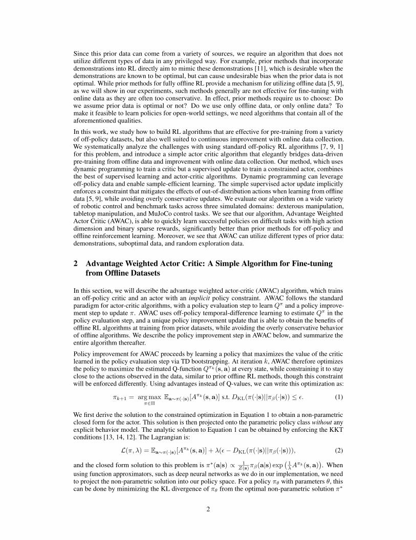
6.1) Comparative Evaluation on Dexterous Manipulation Tasks. We aim to study tasks represen-tative of the difficulties of real-world robot learning, where offline learning and online fine-tuning aremost relevant. One such setting is the suite of dexterous manipulation tasks proposed by Rajeswaranet al. [15]. These tasks involve complex manipulation skills using a 28-DoF five-fingered hand in theMuJoCo simulator [18] shown in Figure 1: in-hand rotation of a pen, opening a door by unlatching

3

Succ

ess

Rat

e

0K 200K 400K 600K 800KTimesteps

0.0

0.2

0.4

0.6

0.8

1.0 pen-binary-v0

0K 200K 400K 600K 800KTimesteps

0.0

0.2

0.4

0.6

0.8

1.0 door-binary-v0

0M 1M 2M 3M 4MTimesteps

0.0

0.2

0.4

0.6

0.8

1.0 relocate-binary-v0

AWAC (Ours) ABM [40] AWR [32] BEAR [23] BRAC [50] DAPG [37] SACfD [45] SAC+BC [30]

Figure 1: Comparative evaluation on the dexterous manipulation tasks. These tasks are difficult due to theirhigh action dimensionality and reward sparsity. We see that AWAC is able to learn these tasks with little onlinedata collection required (100K samples ≈ 16 minutes of equivalent real-world interaction time). Meanwhile,most prior methods are not able to solve the harder two tasks: door opening and object relocation.

the handle, and picking up a sphere and relocating it to a target location. These environmentsexhibit many challenges: high dimensional action spaces, complex manipulation physics with manyintermittent contacts, and randomized hand and object positions. The reward functions in theseenvironments are binary 0-1 rewards for task completion. 1 Rajeswaran et al. [15] provide 25 humandemonstrations for each task, which are not fully optimal but do solve the task. Since this dataset isvery small, we generated another 500 trajectories with behavior cloning.

0K 20K 40K 60K 80K 100KTimesteps

0.0

0.2

0.4

0.6

0.8

1.0

Succ

ess R

ate

Learning From Random Data

AWACBEAR

BRACABM

SACSAC+BC

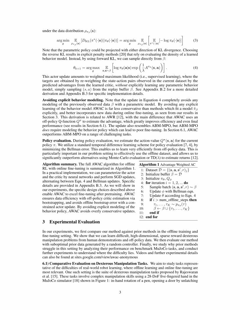
Figure 2: Comparison offine-tuning from an initialdataset of suboptimal dataon a robot pushing task.

First, we compare our method on the dexterous manipulation tasksdescribed earlier against prior methods for off-policy learning, offlinelearning, and bootstrapping from demonstrations. Specific implemen-tation details are discussed in Appendix B.4. The results are shown inFig. 1. Our method is able to leverage the prior data to quickly attaingood performance, and the efficient off-policy actor-critic componentof our approach fine-tunes much more quickly than demonstration aug-mented policy gradient (DAPG), the method proposed by Rajeswaranet al. [15]. For example, our method solves the pen task in 120Ktimesteps, the equivalent of just 20 minutes of online interaction. Whilethe baseline comparisons and ablations are able to make some amountof progress on the pen task, alternative off-policy RL and offline RLalgorithms are largely unable to solve the door and relocate task inthe time-frame considered. We find that the design decisions to useoff-policy critic estimation allow AWAC to significantly outperformAWR [12] while the implicit behavior modeling allows AWAC to significantly outperform ABM [17],although ABM does make some progress. Rajeswaran et al. [15] show that DAPG can eventuallysolve these tasks with more reward information, but this highlights the weakness of on-policy methodsin sparse reward scenarios. Similar results hold true in benchmark Gym environments; due to spaceconstraints, we present these results in the appendix.

6.2) Fine-Tuning from Random Policy Data. An advantage of using off-policy RL for reinforce-ment learning is that we can also incorporate suboptimal data, rather than only demonstrations. In thisexperiment, we evaluate on a simulated tabletop pushing environment with a Sawyer robot (shown inFig 1), described further in Appendix B.1. To study the potential to learn from suboptimal data, weuse an off-policy dataset of 500 trajectories generated by a random process. The task is to push anobject to a target location in a 40cm x 20cm goal space.

The results are shown in Figure 2. We see that while many methods begin at the same initialperformance, AWAC learns the fastest online and is actually able to make use of the offline dataseteffectively as opposed to some methods which are completely unable to learn.

1Rajeswaran et al. [15] use a combination of task completion factors as the sparse reward. For instance, inthe door task, the sparse reward as a function of the door position d was r = 101d>1.35 + 81d>1.0 + 21d>1.2−0.1||d− 1.57||2. We only use the success measure r = 1d>1.4, which is substantially more difficult.

4

References

[1] Abdolmaleki, A., Springenberg, J. T., Tassa, Y., Munos, R., Heess, N., and Riedmiller, M. Maximuma Posteriori Policy Optimisation. In International Conference on Learning Representations (ICLR), pp.1–19, 2018.

[2] Atkeson, C. G. and Schaal, S. Robot Learning From Demonstration. In International Conference onMachine Learning (ICML), 1997.

[3] Devlin, J., Chang, M.-W., Lee, K., and Toutanova, K. BERT: Pre-training of Deep Bidirectional Trans-formers for Language Understanding. In Association for Compuational Linguistics (ACL), oct 2019.

[4] Fujimoto, S., van Hoof, H., and Meger, D. Addressing Function Approximation Error in Actor-CriticMethods. International Conference on Machine Learning (ICML), 2018.

[5] Fujimoto, S., Meger, D., and Precup, D. Off-Policy Deep Reinforcement Learning without Exploration. InInternational Conference on Machine Learning (ICML), dec 2019.

[6] Gao, Y., Xu, H., Lin, J., Yu, F., Levine, S., and Darrell, T. Reinforcement learning from imperfectdemonstrations. CoRR, abs/1802.05313, 2018.

[7] Haarnoja, T., Zhou, A., Abbeel, P., and Levine, S. Soft Actor-Critic: Off-Policy Maximum Entropy DeepReinforcement Learning with a Stochastic Actor. In International Conference on Machine Learning, 2018.

[8] Krizhevsky, A., Sutskever, I., and Hinton, G. E. Imagenet classification with deep convolutional neuralnetworks. In Advances in Neural Information Processing Systems (NIPS), pp. 1097–1105, 2012.

[9] Kumar, A., Fu, J., Tucker, G., and Levine, S. Stabilizing Off-Policy Q-Learning via Bootstrapping ErrorReduction. In Neural Information Processing Systems (NeurIPS), jun 2019.

[10] Lillicrap, T. P., Hunt, J. J., Pritzel, A., Heess, N., Erez, T., Tassa, Y., Silver, D., and Wierstra, D. Continuouscontrol with deep reinforcement learning. In International Conference on Learning Representations (ICLR),2016. ISBN 0-7803-3213-X. doi: 10.1613/jair.301.

[11] Nair, A., Mcgrew, B., Andrychowicz, M., Zaremba, W., and Abbeel, P. Overcoming Exploration inReinforcement Learning with Demonstrations. In IEEE International Conference on Robotics andAutomation (ICRA), 2018.

[12] Peng, X. B., Kumar, A., Zhang, G., and Levine, S. Advantage-Weighted Regression: Simple and ScalableOff-Policy Reinforcement Learning. sep 2019.

[13] Peters, J. and Schaal, S. Reinforcement Learning by Reward-weighted Regression for Operational SpaceControl. In International Conference on Machine Learning, 2007.

[14] Peters, J., Mülling, K., and Altün, Y. Relative Entropy Policy Search. In AAAI Conference on ArtificialIntelligence, pp. 1607–1612, 2010.

[15] Rajeswaran, A., Kumar, V., Gupta, A., Schulman, J., Todorov, E., and Levine, S. Learning ComplexDexterous Manipulation with Deep Reinforcement Learning and Demonstrations. In Robotics: Scienceand Systems, 2018.

[16] Schaal, S. Learning from demonstration. In Advances in Neural Information Processing Systems (NeurIPS),number 9, pp. 1040–1046, 1997. ISBN 1558604863. doi: 10.1016/j.robot.2004.03.001.

[17] Siegel, N. Y., Springenberg, J. T., Berkenkamp, F., Abdolmaleki, A., Neunert, M., Lampe, T., Hafner,R., Heess, N., and Riedmiller, M. Keep doing what worked: Behavioral modelling priors for offlinereinforcement learning, 2020.

[18] Todorov, E., Erez, T., and Tassa, Y. MuJoCo: A physics engine for model-based control. In IEEE/RSJInternational Conference on Intelligent Robots and Systems (IROS), pp. 5026–5033, 2012. ISBN9781467317375. doi: 10.1109/IROS.2012.6386109.

[19] Vecerík, M., Hester, T., Scholz, J., Wang, F., Pietquin, O., Piot, B., Heess, N., Rothörl, T., Lampe, T., andRiedmiller, M. Leveraging Demonstrations for Deep Reinforcement Learning on Robotics Problems withSparse Rewards. CoRR, abs/1707.0, 2017.

[20] Wu, Y., Tucker, G., and Nachum, O. Behavior Regularized Offline Reinforcement Learning. In Interna-tional Conference on Learning Representations (ICLR), nov 2020.

[21] Zhou, A., Jang, E., Kappler, D., Herzog, A., Khansari, M., Wohlhart, P., Bai, Y., Kalakrishnan, M., Levine,S., and Finn, C. Watch, try, learn: Meta-learning from demonstrations and reward. CoRR, abs/1906.03352,2019.

5

Ave

rage

Ret

urn

0K 100K 200K 300K 400K 500KTimesteps

0

2000

4000

6000

8000

10000 HalfCheetah-v2

0K 100K 200K 300K 400K 500KTimesteps

2000

0

2000

4000

6000 Ant-v2

0K 100K 200K 300K 400K 500KTimesteps

0

2000

4000

Walker2d-v2

AWAC (Ours) ABM [40] AWR [32] BEAR [23] BRAC [50] DAPG [37] SACfD [45] SAC+BC [30]

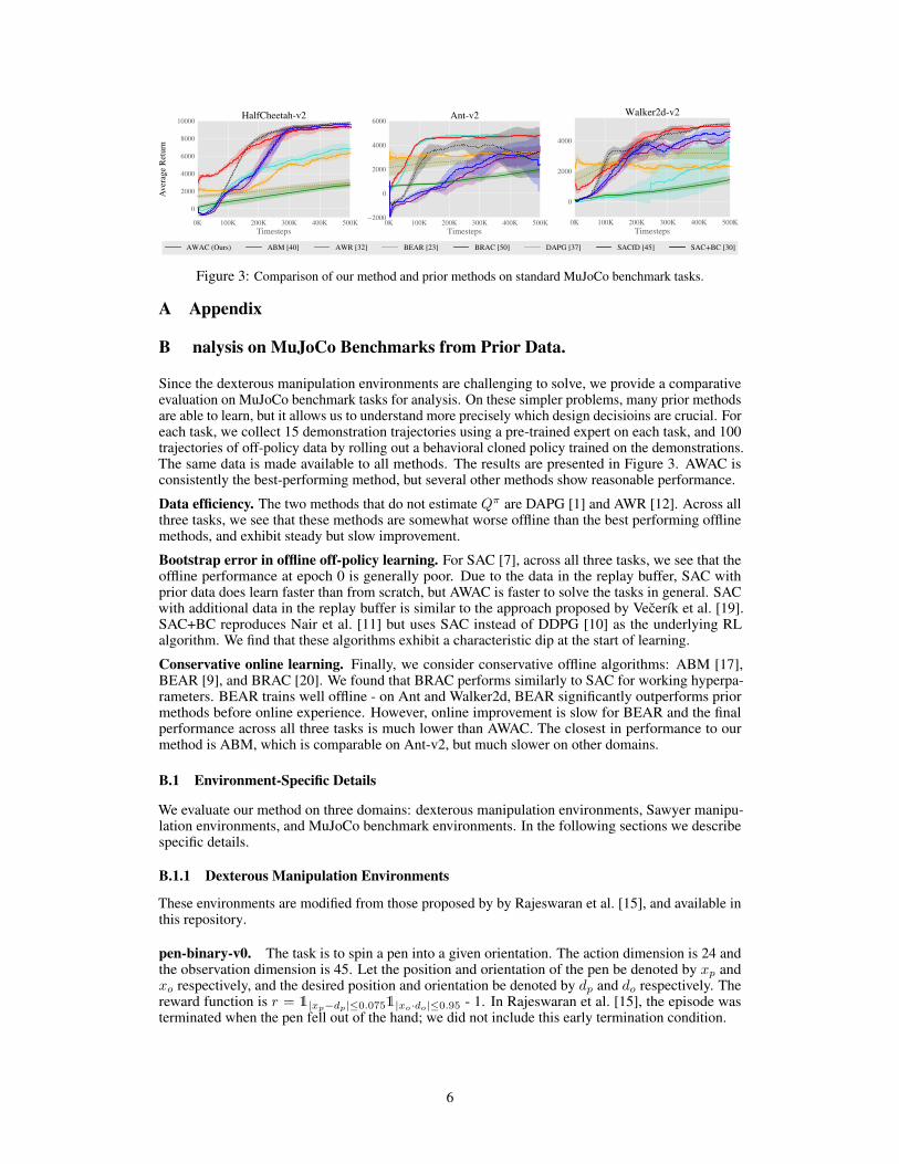
Figure 3: Comparison of our method and prior methods on standard MuJoCo benchmark tasks.

A Appendix

B nalysis on MuJoCo Benchmarks from Prior Data.

Since the dexterous manipulation environments are challenging to solve, we provide a comparativeevaluation on MuJoCo benchmark tasks for analysis. On these simpler problems, many prior methodsare able to learn, but it allows us to understand more precisely which design decisioins are crucial. Foreach task, we collect 15 demonstration trajectories using a pre-trained expert on each task, and 100trajectories of off-policy data by rolling out a behavioral cloned policy trained on the demonstrations.The same data is made available to all methods. The results are presented in Figure 3. AWAC isconsistently the best-performing method, but several other methods show reasonable performance.

Data efficiency. The two methods that do not estimate Qπ are DAPG [1] and AWR [12]. Across allthree tasks, we see that these methods are somewhat worse offline than the best performing offlinemethods, and exhibit steady but slow improvement.

Bootstrap error in offline off-policy learning. For SAC [7], across all three tasks, we see that theoffline performance at epoch 0 is generally poor. Due to the data in the replay buffer, SAC withprior data does learn faster than from scratch, but AWAC is faster to solve the tasks in general. SACwith additional data in the replay buffer is similar to the approach proposed by Vecerík et al. [19].SAC+BC reproduces Nair et al. [11] but uses SAC instead of DDPG [10] as the underlying RLalgorithm. We find that these algorithms exhibit a characteristic dip at the start of learning.

Conservative online learning. Finally, we consider conservative offline algorithms: ABM [17],BEAR [9], and BRAC [20]. We found that BRAC performs similarly to SAC for working hyperpa-rameters. BEAR trains well offline - on Ant and Walker2d, BEAR significantly outperforms priormethods before online experience. However, online improvement is slow for BEAR and the finalperformance across all three tasks is much lower than AWAC. The closest in performance to ourmethod is ABM, which is comparable on Ant-v2, but much slower on other domains.

B.1 Environment-Specific Details

We evaluate our method on three domains: dexterous manipulation environments, Sawyer manipu-lation environments, and MuJoCo benchmark environments. In the following sections we describespecific details.

B.1.1 Dexterous Manipulation Environments

These environments are modified from those proposed by by Rajeswaran et al. [15], and available inthis repository.

pen-binary-v0. The task is to spin a pen into a given orientation. The action dimension is 24 andthe observation dimension is 45. Let the position and orientation of the pen be denoted by xp andxo respectively, and the desired position and orientation be denoted by dp and do respectively. Thereward function is r = 1|xp−dp|≤0.0751|xo·do|≤0.95 - 1. In Rajeswaran et al. [15], the episode wasterminated when the pen fell out of the hand; we did not include this early termination condition.

6

door-binary-v0. The task is to open a door, which requires first twisting a latch. The actiondimension is 28 and the observation dimension is 39. Let d denote the angle of the door. The rewardfunction is r = 1d>1.4 - 1.

relocate-binary-v0. The task is to relocate an object to a goal location. The action dimension is30 and the observation dimension is 39. Let xp denote the object position and dp denote the desiredposition. The reward is r = 1|xp−dp|≤0.1 - 1.

B.1.2 Sawyer Manipulation Environment

SawyerPush-v0. This environment is included in the Multiworld library. The task is to push apuck to a goal position in a 40cm x 20cm, and the reward function is the negative distance betweenthe puck and goal position. When using this environment, we use hindsight experience replay forgoal-conditioned reinforcement learning. The random dataset for prior data was collected by rollingout an Ornstein-Uhlenbeck process with θ = 0.15 and σ = 0.3.

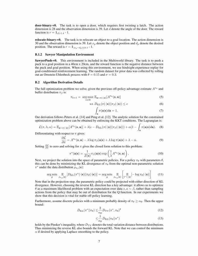
B.2 Algorithm Derivation Details

The full optimization problem we solve, given the previous off-policy advantage estimate Aπk andbuffer distribution πβ is:

πk+1 = argmaxπ∈Π

Ea∼π(·|s)[Aπk(s,a)] (5)

s.t. DKL(π(·|s)||πβ(·|s)) ≤ ε (6)∫a

π(a|s)da = 1. (7)

Our derivation follows Peters et al. [14] and Peng et al. [12]. The analytic solution for the constrainedoptimization problem above can be obtained by enforcing the KKT conditions. The Lagrangian is:

L(π, λ, α) = Ea∼π(·|s)[Aπk(s,a)] + λ(ε−DKL(π(·|s)||πβ(·|s))) + α(1−

∫a

π(a|s)da). (8)

Differentiating with respect to π gives:∂L∂π

= Aπk(s,a)− λ log πβ(a|s) + λ log π(a|s) + λ− α. (9)

Setting ∂L∂π to zero and solving for π gives the closed form solution to this problem:

π∗(a|s) = 1

Z(s)πβ(a|s) exp

(1

λAπk(s,a)

), (10)

Next, we project the solution into the space of parametric policies. For a policy πθ with parameters θ,this can be done by minimizing the KL divergence of πθ from the optimal non-parametric solutionπ∗ under the data distribution ρπβ (s):

argminθ

Eρπβ (s)

[DKL(π∗(·|s)||πθ(·|s))] = argmin

θE

ρπβ (s)

[E

π∗(·|s)[− log πθ(·|s)]

](11)

Note that in the projection step, the parametric policy could be projected with either direction of KLdivergence. However, choosing the reverse KL direction has a key advantage: it allows us to optimizeθ as a maximum likelihood problem with an expectation over data s, a ∼ β, rather than samplingactions from the policy that may be out of distribution for the Q function. In our experiments weshow that this decision is vital for stable off-policy learning.

Furthermore, assume discrete policies with a minimum probably density of πθ ≥ αθ. Then the upperbound:

DKL(π∗||πθ) ≤

2

αθDTV(π

∗, πθ)2 (12)

≤ 1

αθDKL(πθ||π∗) (13)

holds by the Pinsker’s inequality, whereDTV denotes the total variation distance between distributions.Thus minimizing the reverse KL also bounds the forward KL. Note that we can control the minimumα if desired by applying Laplace smoothing to the policy.

7

Hyper-parameter ValueTraining Batches Per Timestep 1

Exploration Noise None (stochastic policy)RL Batch Size 1024

Discount Factor 0.99Reward Scaling 1

Replay Buffer Size 1000000Number of pretraining steps 25000

Policy Hidden Sizes [256, 256, 256, 256]Policy Hidden Activation ReLU

Policy Weight Decay 10−4

Policy Learning Rate 3× 10−4

Q Hidden Sizes [256, 256, 256, 256]Q Hidden Activation ReLU

Q Weight Decay 0Q Learning Rate 3× 10−4

Target Network τ 5× 10−3

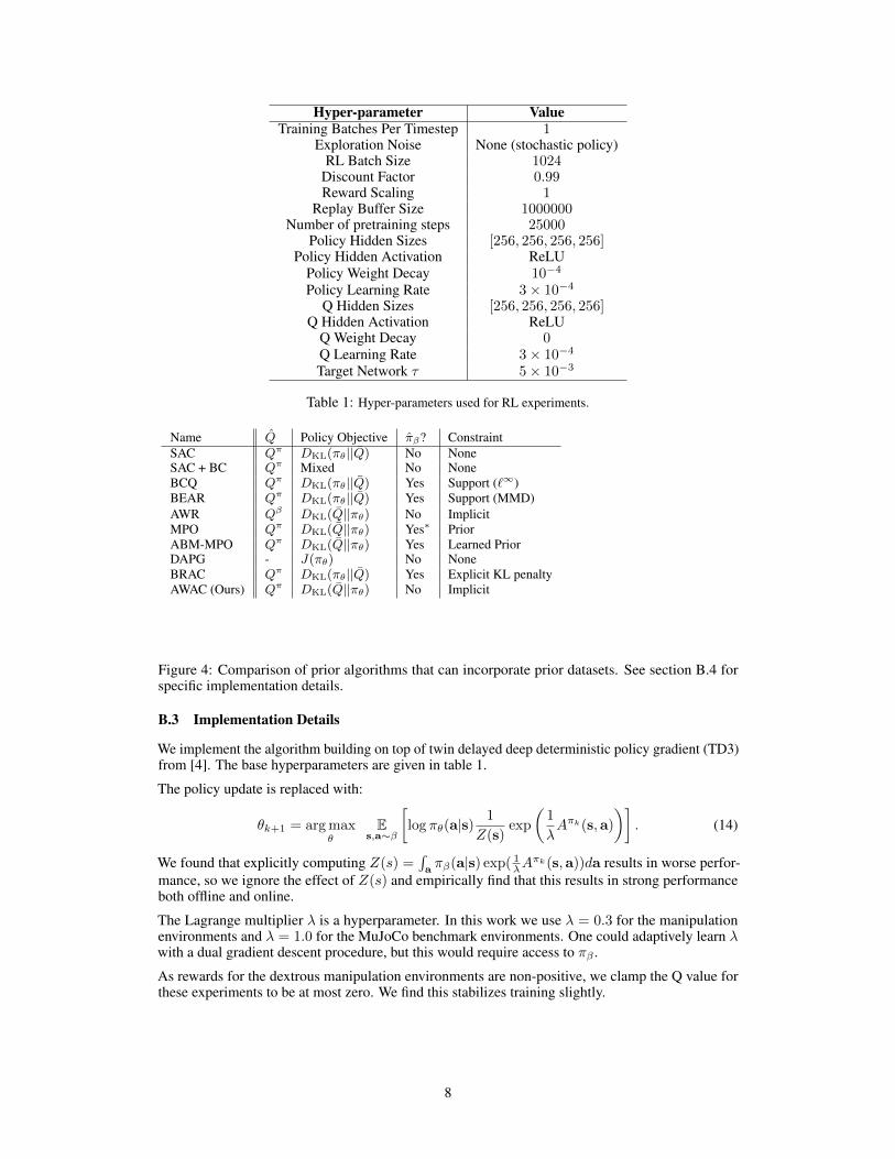
Table 1: Hyper-parameters used for RL experiments.

Name Q Policy Objective πβ? ConstraintSAC Qπ DKL(πθ||Q) No NoneSAC + BC Qπ Mixed No NoneBCQ Qπ DKL(πθ||Q) Yes Support (`∞)BEAR Qπ DKL(πθ||Q) Yes Support (MMD)AWR Qβ DKL(Q||πθ) No ImplicitMPO Qπ DKL(Q||πθ) Yes∗ PriorABM-MPO Qπ DKL(Q||πθ) Yes Learned PriorDAPG - J(πθ) No NoneBRAC Qπ DKL(πθ||Q) Yes Explicit KL penaltyAWAC (Ours) Qπ DKL(Q||πθ) No Implicit

Figure 4: Comparison of prior algorithms that can incorporate prior datasets. See section B.4 forspecific implementation details.

B.3 Implementation Details

We implement the algorithm building on top of twin delayed deep deterministic policy gradient (TD3)from [4]. The base hyperparameters are given in table 1.

The policy update is replaced with:

θk+1 = argmaxθ

Es,a∼β

[log πθ(a|s)

1

Z(s)exp

(1

λAπk(s,a)

)]. (14)

We found that explicitly computing Z(s) =∫aπβ(a|s) exp( 1

λAπk(s,a))da results in worse perfor-

mance, so we ignore the effect of Z(s) and empirically find that this results in strong performanceboth offline and online.

The Lagrange multiplier λ is a hyperparameter. In this work we use λ = 0.3 for the manipulationenvironments and λ = 1.0 for the MuJoCo benchmark environments. One could adaptively learn λwith a dual gradient descent procedure, but this would require access to πβ .

As rewards for the dextrous manipulation environments are non-positive, we clamp the Q value forthese experiments to be at most zero. We find this stabilizes training slightly.

8

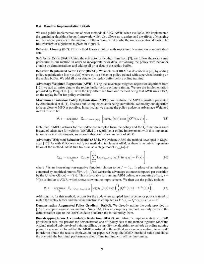
B.4 Baseline Implementation Details

We used public implementations of prior methods (DAPG, AWR) when available. We implementedthe remaining algorithms in our framework, which also allows us to understand the effects of changingindividual components of the method. In the section, we describe the implementation details. Thefull overview of algorithms is given in Figure 4.

Behavior Cloning (BC). This method learns a policy with supervised learning on demonstrationdata.

Soft Actor Critic (SAC). Using the soft actor critic algorithm from [7], we follow the exact sameprocedure as our method in order to incorporate prior data, initializing the policy with behaviorcloning on demonstrations and adding all prior data to the replay buffer.

Behavior Regularized Actor Critic (BRAC). We implement BRAC as described in [20] by addingpolicy regularization log(πβ(a|s)) where πβ is a behavior policy trained with supervised learning onthe replay buffer. We add all prior data to the replay buffer before online training.

Advantage Weighted Regression (AWR). Using the advantage weighted regression algorithm from[12], we add all prior data to the replay buffer before online training. We use the implementationprovided by Peng et al. [12], with the key difference from our method being that AWR uses TD(λ)on the replay buffer for policy evaluation.

Maximum a Posteriori Policy Optimization (MPO). We evaluate the MPO algorithm presentedby Abdolmaleki et al. [1]. Due to a public implementation being unavailable, we modify our algorithmto be as close to MPO as possible. In particular, we change the policy update in Advantage WeightedActor Critic to be:

θi ←− argmaxθi

Es∼D,a∼π(a|s)

[log πθi(a|s) exp(

1

βQπβ (s, a))

]. (15)

Note that in MPO, actions for the update are sampled from the policy and the Q-function is usedinstead of advantage for weights. We failed to see offline or online improvement with this implemen-tation in most environments, so we omit this comparison in favor of ABM.

Advantage-Weighted Behavior Model (ABM). We evaluate ABM, the method developed in Siegelet al. [17]. As with MPO, we modify our method to implement ABM, as there is no public implemen-tation of the method. ABM first trains an advantage model πθabm(a|s):

θabm = argmaxθi

Eτ∼D

|τ |∑t=1

log πθabm(at|st)f(R(τt:N )− V (s))

. (16)

where f is an increasing non-negative function, chosen to be f = 1+. In place of an advantagecomputed by empirical returnsR(τt:N )−V (s) we use the advantage estimate computed per transitionby the Q value Q(s, a)− V (s). This is favorable for running ABM online, as computing R(τt:N )−V (s) is similar to AWR, which shows slow online improvement. We then use the policy update:

θi ←− argmaxθi

Es∼D,a∼πabm(a|s)

[log πθi(a|s) exp

(1

λ(Qπi(s, a)− V πi(s))

)]. (17)

Additionally, for this method, actions for the update are sampled from a behavior policy trained tomatch the replay buffer and the value function is computed as V π(s) = Qπ(s, a) s.t. a ∼ π.

Demonstration Augmented Policy Gradient (DAPG). We directly utilize the code provided in[15] to compare against our method. Since DAPG is an on-policy method, we only provide thedemonstration data to the DAPG code to bootstrap the initial policy from.

Bootstrapping Error Accumulation Reduction (BEAR). We utilize the implementation of BEARprovided in rlkit. We provide the demonstration and off-policy data to the method together. Since theoriginal method only involved training offline, we modify the algorithm to include an online trainingphase. In general we found that the MMD constraint in the method was too conservative. As a result,in order to obtain the results displayed in our paper, we swept the MMD threshold value and chosethe one with the best final performance after offline training with offline fine-tuning.

9