1876-6102 © 2016 The Authors. Published by Elsevier Ltd. This is an open access article under the CC BY-NC-ND license (http://creativecommons.org/licenses/by-nc-nd/4.0/).Peer-review under responsibility of SINTEF Energi ASdoi: 10.1016/j.egypro.2016.09.187

Energy Procedia 94 ( 2016 ) 37 – 44

ScienceDirect

13th Deep Sea Offshore Wind R&D Conference, EERA DeepWind'2016, 20-22 January 2016, Trondheim, Norway

Offshore Wind Energy Analysis of Cyclone Xaver over North Europe

Konstantinos Christakosa,*, Ioannis Cheliotisb, George Varlasc,d, Gert-Jan Steeneveldb a Uni Research Polytec AS, Sørhauggata 128, 5527 Haugesund, Norway

b Meteorology and Air Quality Section, Wageningen University, 6700AA Wageningen, The Netherlands c Department of Geography, Harokopion University of Athens (HUA), El. Venizelou Str. 70, 17671 Athens, Greece

d Institute of Marine Biological Resources and Inland Waters, Hellenic Centre for Marine Research (HCMR), 19013 Anavissos, Attica, Greece

Abstract

Cyclone Xaver (5 December 2013; North Sea) was an extreme weather event which affected northern Europe, yielding a record of wind power generation. The most striking aspects of this atmospheric phenomenon were the gale-force winds and the upcoming abrupt increase of the wind power over the North Sea. The main objective of the study is the analysis of the impact of Xaver on offshore wind power production. In this way, the WRF numerical model was used to simulate the cyclone in a fine horizontal resolution (5km x 5km). The focus of the simulation is on the extended region of the North Sea and the Baltic Sea. The evaluation of the model outputs against observational data from 3 offshore locations denotes a sufficient agreement (SI 0.12) and supports a realistic analysis of the wind field. The simulation exposed much higher values for wind speed over the North Sea compared to the neighboring regions during the passage of the cyclone. The wind speed at the 100 m level ranged within 11-25 m/s (rated output wind speed) for 40 hours over the North Sea and 70 hours over the Baltic Sea. On the other hand, the wind speed at 100 m exceeded 25 m/s (cut out wind speed) for ca 30 hours over the North Sea. In addition, comparison of wind power density between two different height levels (100 m and 200 m) is presented. The model results indicate 15% to 20% higher wind power density at 200 m than for 100 m for the largest part of the North Sea. For some regions the difference exceeds 25%. © 2016 The Authors. Published by Elsevier Ltd. Peer-review under responsibility of SINTEF Energi AS.

Keywords: Wind Power; Offshore Wind Energy; North Sea; Baltic Sea; Cyclone Xaver; Bodil; Sven

* Corresponding author.

E-mail address: Konstantinos.Christakos@polytec.no

Available online at www.sciencedirect.com

© 2016 The Authors. Published by Elsevier Ltd. This is an open access article under the CC BY-NC-ND license (http://creativecommons.org/licenses/by-nc-nd/4.0/).Peer-review under responsibility of SINTEF Energi AS

38 Konstantinos Christakos et al. / Energy Procedia 94 ( 2016 ) 37 – 44

1. Introduction

On 4 December, 2013 a cyclonic system was generated southeasterly of Greenland. During its formation, the upper air conditions intensified the cyclonic circulation and the system progressed southeasterly. The cyclone known as Xaver by Free University of Berlin [1] (also known as Bodil [2], [3] by Danish Meteorological Institute and Sven [4] by Swedish Meteorological and Hydrological Institute) was continuously deepening during its movement towards Scandinavian Peninsula. In total, Xaver influenced an extensive region of North Europe, moving gradually from southeastern Greenland to the Baltic Sea, passing over the north shore of United Kingdom, the North Sea and Scandinavia. It was a remarkable phenomenon as it was accompanied by gale-force winds over North Sea and low values of mean sea level pressure in the center.

The impact of the strong winds was substantial mainly for the coastal areas of North Europe. The intensity of the wind field had a major impact in the energy industry. The wind resources affected the safety and performance of the grid [5]. Thousands of households encountered electricity problems [6], whereas in Germany onshore and offshore wind turbines set wind energy production records higher than 26000 MW [7] causing decrease of power spot prices lower than 25 €/MWh [8]. Moreover, in Denmark the shutdown of the wind turbines due to extreme wind speeds together with high electricity consumption led to a significant increase in the power spot prices up to 580 DKK/MWh [5].

This study aims to investigate the impact of offshore wind energy of Cyclone Xaver over the North Sea and the Baltic Sea. Additionally, the ability of a numerical model to simulate the event with respect to this aspect is tested. Weather Research & Forecasting (WRF) model has been used in the past for offshore wind energy applications with satisfying results for wind climatology [9] [10] [11] [12]. These evaluation studies have been focused mainly on average wind speed. Here we will extend the model evaluation to extreme wind conditions. Thus, the WRF numerical model was utilized for the simulation of Xaver and for a better representation of the physical and dynamical conditions which supported the development and determined the track of the system. The time period under study expands from 4 December, 2013 00:00 UTC to 7 December, 2013 12:00 UTC. The focus is on the extended region of the Baltic Sea and the North Sea, home of the largest operational offshore wind farms in the world [13].

2. Theoretical Background

2.1. Wind Power Density

The wind power density (WPD), measured in W/m2, is estimated for the investigation of the event [14]. It is used as an indication of the wind energy available for conversion by wind turbines during the cyclone’s passage. It is a function of the air density (ρ) and the third power of the wind speed (U).

3

21

UWPD (1)

Offshore areas of North Europe such as the North Sea and the Baltic Sea show high WPD values. The annual

mean value for WPD at these areas is higher than 650 W/m2 at 100 m and 900 W/m2 at 200 m [15].

2.2. Wind Turbines and Wind Speed

A wind turbine starts to rotate its blades and generate power for wind speed usually greater than 3 m/s, known as cut-in wind speed. As the wind speed increases, the level of generated power raises until reaches the turbine generation limit. The wind speed at which this limit is reached, called the rated output wind speed and it is typically at 11-12 m/s [16] [17]. Wind turbines tend to perform to their utmost capacity regarding wind power generation at the 11-25 m/s range. The 25 m/s threshold is typically the cut out wind speed and it is defined as the speed at which the wind turbines stop rotating to avoid damage [18].

Konstantinos Christakos et al. / Energy Procedia 94 ( 2016 ) 37 – 44 39

3. Case Study

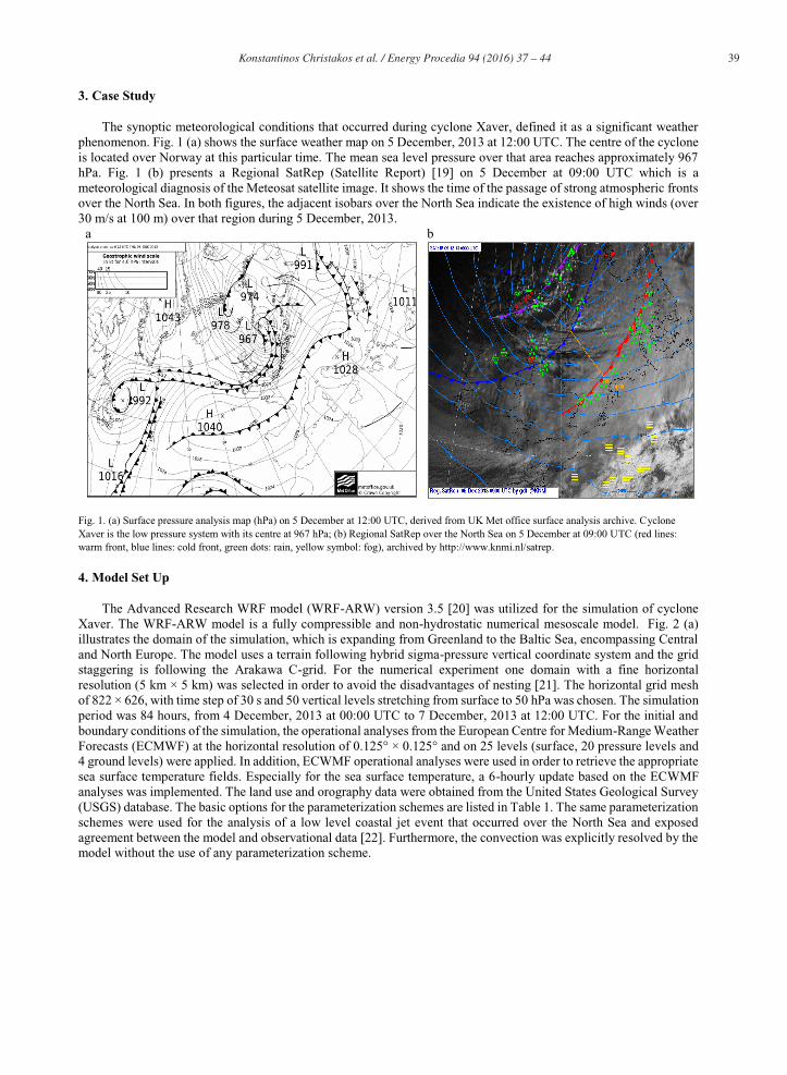
The synoptic meteorological conditions that occurred during cyclone Xaver, defined it as a significant weather phenomenon. Fig. 1 (a) shows the surface weather map on 5 December, 2013 at 12:00 UTC. The centre of the cyclone is located over Norway at this particular time. The mean sea level pressure over that area reaches approximately 967 hPa. Fig. 1 (b) presents a Regional SatRep (Satellite Report) [19] on 5 December at 09:00 UTC which is a meteorological diagnosis of the Meteosat satellite image. It shows the time of the passage of strong atmospheric fronts over the North Sea. In both figures, the adjacent isobars over the North Sea indicate the existence of high winds (over 30 m/s at 100 m) over that region during 5 December, 2013.

a b

Fig. 1. (a) Surface pressure analysis map (hPa) on 5 December at 12:00 UTC, derived from UK Met office surface analysis archive. Cyclone Xaver is the low pressure system with its centre at 967 hPa; (b) Regional SatRep over the North Sea on 5 December at 09:00 UTC (red lines: warm front, blue lines: cold front, green dots: rain, yellow symbol: fog), archived by http://www.knmi.nl/satrep.

4. Model Set Up

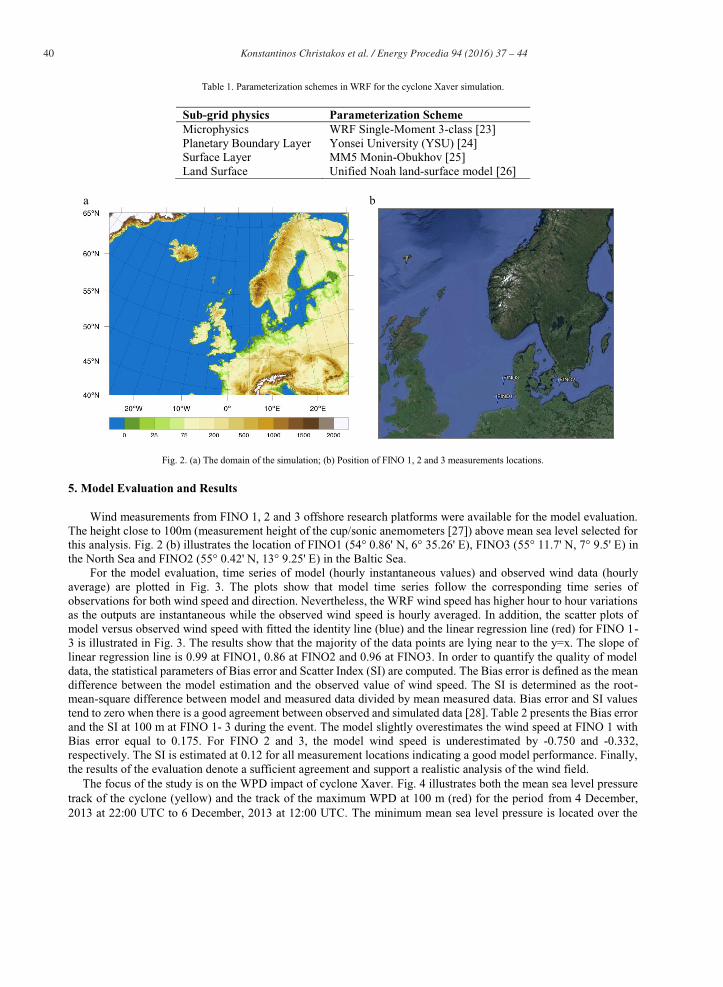
The Advanced Research WRF model (WRF-ARW) version 3.5 [20] was utilized for the simulation of cyclone Xaver. The WRF-ARW model is a fully compressible and non-hydrostatic numerical mesoscale model. Fig. 2 (a) illustrates the domain of the simulation, which is expanding from Greenland to the Baltic Sea, encompassing Central and North Europe. The model uses a terrain following hybrid sigma-pressure vertical coordinate system and the grid staggering is following the Arakawa C-grid. For the numerical experiment one domain with a fine horizontal resolution (5 km × 5 km) was selected in order to avoid the disadvantages of nesting [21]. The horizontal grid mesh of 822 × 626, with time step of 30 s and 50 vertical levels stretching from surface to 50 hPa was chosen. The simulation period was 84 hours, from 4 December, 2013 at 00:00 UTC to 7 December, 2013 at 12:00 UTC. For the initial and boundary conditions of the simulation, the operational analyses from the European Centre for Medium-Range Weather Forecasts (ECMWF) at the horizontal resolution of 0.125° × 0.125° and on 25 levels (surface, 20 pressure levels and 4 ground levels) were applied. In addition, ECWMF operational analyses were used in order to retrieve the appropriate sea surface temperature fields. Especially for the sea surface temperature, a 6-hourly update based on the ECWMF analyses was implemented. The land use and orography data were obtained from the United States Geological Survey (USGS) database. The basic options for the parameterization schemes are listed in Table 1. The same parameterization schemes were used for the analysis of a low level coastal jet event that occurred over the North Sea and exposed agreement between the model and observational data [22]. Furthermore, the convection was explicitly resolved by the model without the use of any parameterization scheme.

40 Konstantinos Christakos et al. / Energy Procedia 94 ( 2016 ) 37 – 44

Table 1. Parameterization schemes in WRF for the cyclone Xaver simulation.

Sub-grid physics Parameterization Scheme Microphysics WRF Single-Moment 3-class [23] Planetary Boundary Layer Yonsei University (YSU) [24] Surface Layer MM5 Monin-Obukhov [25] Land Surface Unified Noah land-surface model [26]

a b

Fig. 2. (a) The domain of the simulation; (b) Position of FINO 1, 2 and 3 measurements locations.

5. Model Evaluation and Results

Wind measurements from FINO 1, 2 and 3 offshore research platforms were available for the model evaluation. The height close to 100m (measurement height of the cup/sonic anemometers [27]) above mean sea level selected for this analysis. Fig. 2 (b) illustrates the location of FINO1 (54° 0.86' N, 6° 35.26' E), FINO3 (55° 11.7' N, 7° 9.5' E) in the North Sea and FINO2 (55° 0.42' N, 13° 9.25' E) in the Baltic Sea.

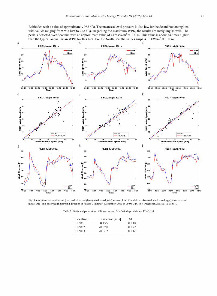
For the model evaluation, time series of model (hourly instantaneous values) and observed wind data (hourly average) are plotted in Fig. 3. The plots show that model time series follow the corresponding time series of observations for both wind speed and direction. Nevertheless, the WRF wind speed has higher hour to hour variations as the outputs are instantaneous while the observed wind speed is hourly averaged. In addition, the scatter plots of model versus observed wind speed with fitted the identity line (blue) and the linear regression line (red) for FINO 1-3 is illustrated in Fig. 3. The results show that the majority of the data points are lying near to the y=x. The slope of linear regression line is 0.99 at FINO1, 0.86 at FINO2 and 0.96 at FINO3. In order to quantify the quality of model data, the statistical parameters of Bias error and Scatter Index (SI) are computed. The Bias error is defined as the mean difference between the model estimation and the observed value of wind speed. The SI is determined as the root-mean-square difference between model and measured data divided by mean measured data. Bias error and SI values tend to zero when there is a good agreement between observed and simulated data [28]. Table 2 presents the Bias error and the SI at 100 m at FINO 1- 3 during the event. The model slightly overestimates the wind speed at FINO 1 with Bias error equal to 0.175. For FINO 2 and 3, the model wind speed is underestimated by -0.750 and -0.332, respectively. The SI is estimated at 0.12 for all measurement locations indicating a good model performance. Finally, the results of the evaluation denote a sufficient agreement and support a realistic analysis of the wind field.

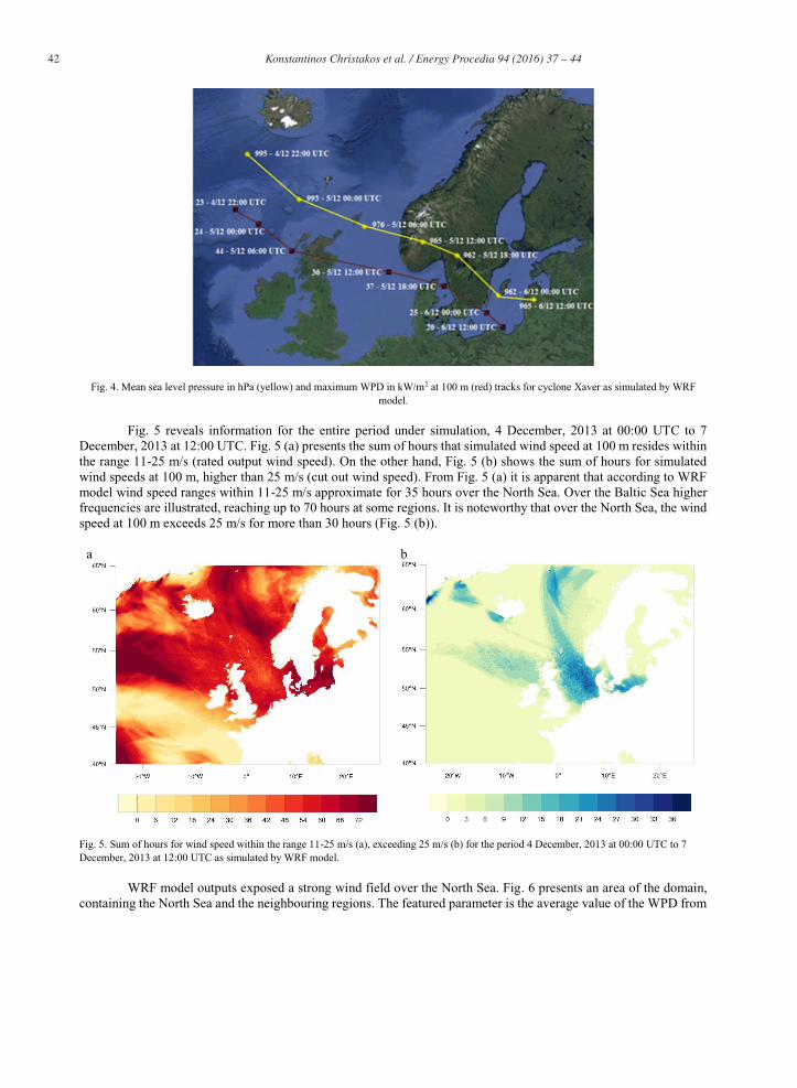
The focus of the study is on the WPD impact of cyclone Xaver. Fig. 4 illustrates both the mean sea level pressure track of the cyclone (yellow) and the track of the maximum WPD at 100 m (red) for the period from 4 December, 2013 at 22:00 UTC to 6 December, 2013 at 12:00 UTC. The minimum mean sea level pressure is located over the

Konstantinos Christakos et al. / Energy Procedia 94 ( 2016 ) 37 – 44 41

Baltic Sea with a value of approximately 962 hPa. The mean sea level pressure is also low for the Scandinavian regions with values ranging from 965 hPa to 962 hPa. Regarding the maximum WPD, the results are intriguing as well. The peak is detected over Scotland with an approximate value of 43.9 kW/m2 at 100 m. This value is about 54 times higher than the typical annual mean WPD for this area. For the North Sea, the values surpass 36 kW/m2 at 100 m.

a b c

d e f

g h i

Fig. 3. (a-c) time series of model (red) and observed (blue) wind speed; (d-f) scatter plots of model and observed wind speed; (g-i) time series of model (red) and observed (blue) wind direction at FINO1-3 during 4 December, 2013 at 00:00 UTC to 7 December, 2013 at 12:00 UTC.

Table 2. Statistical parameters of Bias error and SI of wind speed data at FINO 1-3

Location Bias error [m/s] SI FINO1 0.175 0.118 FINO2 -0.750 0.122 FINO3 -0.332 0.116

42 Konstantinos Christakos et al. / Energy Procedia 94 ( 2016 ) 37 – 44

Fig. 4. Mean sea level pressure in hPa (yellow) and maximum WPD in kW/m2 at 100 m (red) tracks for cyclone Xaver as simulated by WRF model.

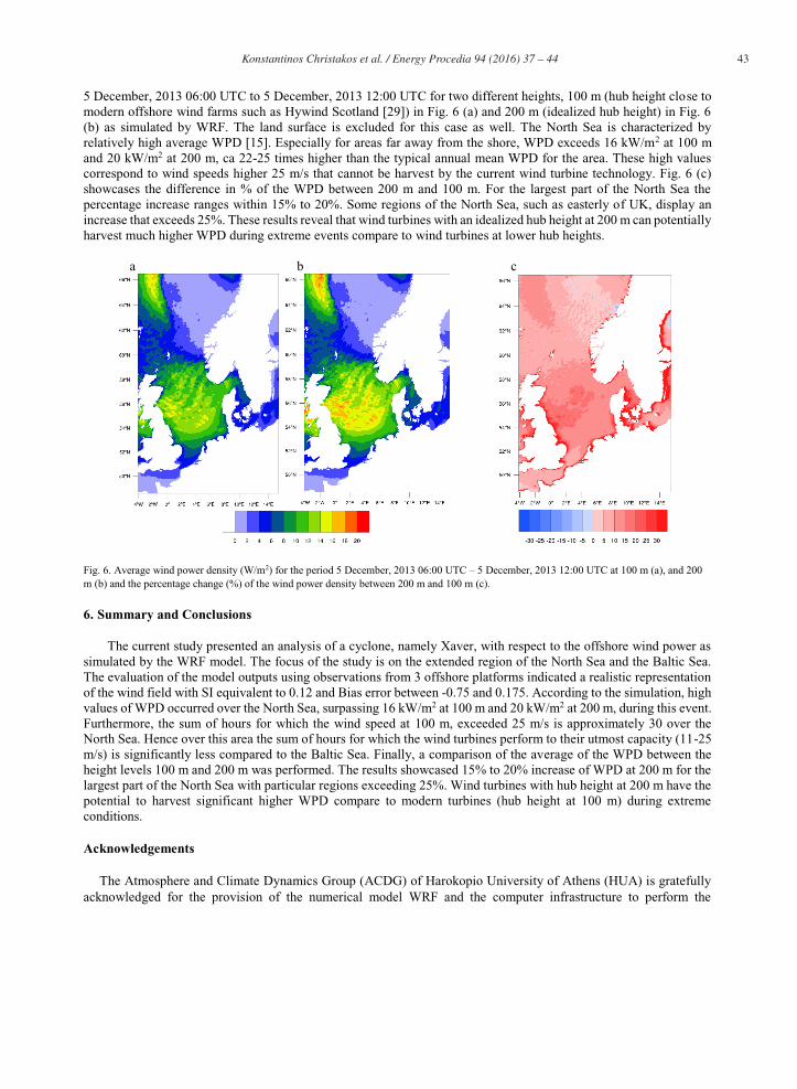
Fig. 5 reveals information for the entire period under simulation, 4 December, 2013 at 00:00 UTC to 7 December, 2013 at 12:00 UTC. Fig. 5 (a) presents the sum of hours that simulated wind speed at 100 m resides within the range 11-25 m/s (rated output wind speed). On the other hand, Fig. 5 (b) shows the sum of hours for simulated wind speeds at 100 m, higher than 25 m/s (cut out wind speed). From Fig. 5 (a) it is apparent that according to WRF model wind speed ranges within 11-25 m/s approximate for 35 hours over the North Sea. Over the Baltic Sea higher frequencies are illustrated, reaching up to 70 hours at some regions. It is noteworthy that over the North Sea, the wind speed at 100 m exceeds 25 m/s for more than 30 hours (Fig. 5 (b)).

a b

Fig. 5. Sum of hours for wind speed within the range 11-25 m/s (a), exceeding 25 m/s (b) for the period 4 December, 2013 at 00:00 UTC to 7 December, 2013 at 12:00 UTC as simulated by WRF model.

WRF model outputs exposed a strong wind field over the North Sea. Fig. 6 presents an area of the domain, containing the North Sea and the neighbouring regions. The featured parameter is the average value of the WPD from

Konstantinos Christakos et al. / Energy Procedia 94 ( 2016 ) 37 – 44 43

5 December, 2013 06:00 UTC to 5 December, 2013 12:00 UTC for two different heights, 100 m (hub height close to modern offshore wind farms such as Hywind Scotland [29]) in Fig. 6 (a) and 200 m (idealized hub height) in Fig. 6 (b) as simulated by WRF. The land surface is excluded for this case as well. The North Sea is characterized by relatively high average WPD [15]. Especially for areas far away from the shore, WPD exceeds 16 kW/m2 at 100 m and 20 kW/m2 at 200 m, ca 22-25 times higher than the typical annual mean WPD for the area. These high values correspond to wind speeds higher 25 m/s that cannot be harvest by the current wind turbine technology. Fig. 6 (c) showcases the difference in % of the WPD between 200 m and 100 m. For the largest part of the North Sea the percentage increase ranges within 15% to 20%. Some regions of the North Sea, such as easterly of UK, display an increase that exceeds 25%. These results reveal that wind turbines with an idealized hub height at 200 m can potentially harvest much higher WPD during extreme events compare to wind turbines at lower hub heights.

a b c

Fig. 6. Average wind power density (W/m2) for the period 5 December, 2013 06:00 UTC – 5 December, 2013 12:00 UTC at 100 m (a), and 200 m (b) and the percentage change (%) of the wind power density between 200 m and 100 m (c).

6. Summary and Conclusions

The current study presented an analysis of a cyclone, namely Xaver, with respect to the offshore wind power as simulated by the WRF model. The focus of the study is on the extended region of the North Sea and the Baltic Sea. The evaluation of the model outputs using observations from 3 offshore platforms indicated a realistic representation of the wind field with SI equivalent to 0.12 and Bias error between -0.75 and 0.175. According to the simulation, high values of WPD occurred over the North Sea, surpassing 16 kW/m2 at 100 m and 20 kW/m2 at 200 m, during this event. Furthermore, the sum of hours for which the wind speed at 100 m, exceeded 25 m/s is approximately 30 over the North Sea. Hence over this area the sum of hours for which the wind turbines perform to their utmost capacity (11-25 m/s) is significantly less compared to the Baltic Sea. Finally, a comparison of the average of the WPD between the height levels 100 m and 200 m was performed. The results showcased 15% to 20% increase of WPD at 200 m for the largest part of the North Sea with particular regions exceeding 25%. Wind turbines with hub height at 200 m have the potential to harvest significant higher WPD compare to modern turbines (hub height at 100 m) during extreme conditions.

Acknowledgements

The Atmosphere and Climate Dynamics Group (ACDG) of Harokopio University of Athens (HUA) is gratefully acknowledged for the provision of the numerical model WRF and the computer infrastructure to perform the

44 Konstantinos Christakos et al. / Energy Procedia 94 ( 2016 ) 37 – 44

simulations. Wind data from FINO 1, 2 and 3 platforms provided by the research FINO project funded by BMWi (Bundesministerium fuer Wirtschaft und Energie, Federal Ministry for Economic Affairs and Energy) and the PTJ (Projekttraeger Juelich, project executing organization).

References

[1] DWD-Wetterkarte Prognose für Do 05.12.2013, 12:00 UTC, FU Berlin, abgerufen am 20. Dezember 2013 [2] Hansen, Niels (2014) Stormjubilæum - ét år siden Bodil DMI [3] Siewertsen, B., (2013) Stormen hedder Bodil, DMI [4] Wiksten, J., (2013), Stormen Sven på ingång, SMHI [5] Artipoli, G., and F. Durante, (2014), Physical Modeling in Wind Energy Forecasting, DEWI Magazin no. 44 [6] Enoch, N., (2013), Huge storm strikes Europe causing death and destruction and leading to cancelation of hundreds of flights, December

6, 2013, Dailymail online, http://www.dailymail.co.uk [7] Gray, T., (2013), Ireland, U.K., Germany set new wind generation records, December 11, 2013, Into the Wind

(http://www.aweablog.org/) by AWEA [8] Mayer J., (2014), Electricity spot-prices and production data in Germany 2013, Fraunhofer Institute for Solar Energy Systems ISE [9] Krogsaeter, O., and J. Reuder, (2014), Validation of boundary layer parameterization schemes in the weather research and forecasting

model under the aspect of offshore wind energy applications – Part I: Average wind speed and wind shear, Wind Energy, Vol. 18, pp. 769-782

[10] Krogsaeter, O., and J. Reuder, (2014), Validation of boundary layer parameterization schemes in the Weather Research and Forecasting (WRF) model under the aspect of offshore wind energy applications – part II: boundary layer height and atmospheric stability, Wind Energy, Vol. 18, pp. 1291-1302

[11] Draxl, C., Hahmann, A. N., Peña, A. and Giebel, G. (2014), Evaluating winds and vertical wind shear from Weather Research and Forecasting model forecasts using seven planetary boundary layer schemes. Wind Energ., 17: 39–55. doi: 10.1002/we.1555

[12] Barstad, I. (2016) Offshore validation of a 3 km ERA-Interim downscaling—WRF model's performance on static stability. Wind Energ., 19: 515–526. doi: 10.1002/we.1848.

[13] Sun X., D. Huang, and G. Wu, (2012), The current state of offshore wind energy technology development, Energy, Vol. 41, pp. 298-312

[14] Manwell, J. F., J. G. McGowan, and A. L. Rogers, (2010), Wind energy explained: Theory,design and application, 2nd ed. Wiley [15] Faiella, L. M., A. J. Gesino, Management of Meteorological Variables and Wind Mapping. World Wind Energy Association,

http://www.wwindea.org [16] Samsung Renewable Energy Inc., and Pattern Renewable Holdings Canada ULC, (2012), 10 Wind Turbine Specification Report for

Armow Wind Project. [17] Siemens AG Energy Sector, (2011), New dimensions, Siemens Wind Turbine SWT-3.6-107 [18] Shen W. Z., M. B. Montes, P. F. Odgaard, N. K. Poulsen, and H. H. Niemann, (2012), Operation Design of Wind Turbines in Strong

Wind Conditions, EWEA proceedings [19] Debie, F., Regional Satrep: A new way of analyzing the actual weather situation, Koninklijk Nederlands Meteorologisch Instituut,

KNMI, The Netherlands [20] Skamarock, W. C., J. B. Klemp, J. Dudhia, D. O. Gill, D. Barker, M. G. Duda, X.-Y. Huang, and W. Wang, (2008), A description of

the Advanced Research WRF version 3, NCAR Technical Note, TN-468+STR, pp. 113 [21] Warner TT, Peterson RA, Treadon RE., (1997), A tutorial on lateral boundary conditions as a basic and potentially serious limitation to

regional numerical weather prediction, Bull. Am. Meteorol. Soc. 78: 2599–2617. [22] Christakos, K., G. Varlas, J. Reuder, P. Katsafados, and A. Papadopoulos, (2014), Analysis of a Low-level Coastal Jet off the Western

Coast of Norway, Energy Procedia, Vol. 53, pp. 162-172 [23] Hong, S.-Y., J. Dudhia, S.-H. Chen, (2004), A revised approach to ice microphysical processes for the bulk parameterization clouds and

precipitation, Monthly Weather Review, Vol. 132, pp. 103-120, doi: http://dx.doi.org/10.1175/1520 - 0493(2004)132<0103:ARATIM>2.0.CO;2

[24] Hong, S.-Y., Y. Noh, and J. Dudhia, (2006), A new vertical diffusion package with an explicit treatment of entrainment processes, Monthly Weather Review, Vol. 134, pp. 2318-2341, doi: http://dx.doi.org/10.1175/MWR3199.1

[25] Zhang, D.-L., and R. A. Anthes, (1982), A high-resolution model of the planetary boundary layer-sensitivity tests and comparisons with SESAME-79 data, Journal of Applied Meteorology, Vol. 21, pp. 1594-1609

[26] Ek, M. B., K. E. Mitchell, Y. Lin, E. Rogers, P. Grunmann, V. Koren, G. Gayno, and J. D. Tarpley, (2003), Implementation of Noah land surface model advances in the National Centers for Environmental Prediction operational mesoscale Eta model, Journal of Geophysical Research, Vol. 22, doi:10.1029/2002JD003296

[27] Forschungsplattformen in Nord- und Ostsee Nr. 1,2,3, http://www.fino-offshore.de [28] Niclasen, B. A., & Simonsen, K. (2007), Validation of the ECMWF analysis wave data for the area around the Faroe Islands. Societas

Scientiarum Færoensis. [29] Rummelhoff, I., Stephen, B., (2015), Building the world’s first floating offshore wind farm, Statoil ASA