Embed Size (px)
Citation preview
Universidade de Aveiro 2011
Departamento de Electrónica,
Telecomunicações e Informática (DETI)
Paulo Jorge Afonso de Andrade
Distribuição de Sinais OFDM e Vídeo sobre Fibra Distribution of OFDM and Video Signals over Fiber

Universidade de Aveiro 2011
Departamento de Electrónica,
Telecomunicações e Informática (DETI)
Paulo Jorge Afonso de Andrade
Distribuição de Sinais OFDM e Vídeo Sobre Fibra Distribution of OFDM and Video Signals over Fiber
Dissertação apresentada à Universidade de Aveiro para cumprimento dos requisitos necessários à obtenção do grau de Mestre em Engenharia Electrónica e Telecomunicações, realizada sob a orientação científica do Prof. Dr. Mário Lima e do Prof. Dr. António Teixeira, ambos do Departamento de Electrónica, Telecomunicações e Informática e do Instituto de Telecomunicações da Universidade de Aveiro.


Este trabalho é dedicado à minha família e amigos pelo constante apoio e
carinho, estando sempre presente ao longo de todo este percurso.

o júri
presidente Prof. Dr. José Rodrigues Ferreira da Rocha Professor Catedrático do Departamento de Electrónica, Telecomunicações e Informática da Universidade de Aveiro
Prof. Dr. Mário José Neves de Lima
Professor Auxiliar do Departamento de Electrónica, Telecomunicações e Informática da Universidade de Aveiro Prof. Dr. António Luís Jesus Teixeira Professor Associado do Departamento de Electrónica, Telecomunicações e Informática da Universidade de Aveiro
Prof. Dr. Henrique Manuel de Castro Faria Salgado Professor Associado da Faculdade de Engenharia da Universidadade do Porto

agradecimentos
Queria agradecer à minha família pelo incondicional apoio, assim
como a todos os meus amigos, e claro, aos orientadores deste
projecto, o Prof. Doutor Mário José Neves de Lima e Prof. Doutor
António Luís Jesus Teixeira, pelo grande apoio, simpatia, boa
disposição, disponibilidade e vontade de ajudar independentemente
da situação. Um agradecimento também à Universidade de Aveiro
pelas boas condições de aprendizagem prestadas durante estes
últimos anos.

acknowledgment
I want to thank my family, for unconditional support, as well as all my
friends, and of course, the supervisors of this project, Prof. Mário José
Neves de Lima and Prof. António Luís Jesus Teixeira, for all the support,
kindness, good disposition, availability and willingness to help no matter
the situation. I would also like to thank to the Aveiro University for the
good learning conditions always available along these last years.

palavras-chave resumo
Radio sobre fibra (RoF), ultra-wide band (UWB), orthogonal
frequency division multiplexing (OFDM), ECMA-368, ECMA-
387, vídeo digital.
Este trabalho incide na transmissão de sinais de rádio e vídeo
sobre fibra óptica, usando modulação analógica de amplitude, ou
seja sistemas do tipo Radio over Fiber (RoF).
Começamos por descrever alguns dos sinais de rádio e vídeo que
podem beneficiar, em certas aplicações, do recurso a sistemas
RoF. Prosseguimos com a transmissão de sinais OFDM, na
banda das micro-ondas e ondas-milimétricas, de forma a concluir
acerca das vantagens e desvantagens dos vários tipos de
modulação óptica que podemos utilizar no transmissor. Também
focamos a multiplicação de frequência óptica no sentido de
identificar soluções para distribuição de sinais RF de alta
frequência, a baixo custo.
De seguida, dando sequência ao estudo da transmissão dos sinais
OFDM, analisamos alguns dos cenários de transmissão de sinais
WPAN de acordo com os standards ECMA-368 e ECMA-387.
Finalmente, acabamos por estudar brevemente a distribuição de
sinais de vídeo digital sobre fibra usando modulação externa.

keywords
abstract
Radio over Fiber (RoF), ultra-wide band (UWB), orthogonal
frequency division multiplexing (OFDM), ECMA-368, ECMA-
387, digital video.
This work focuses on the transmission of radio and video signals
over fiber using analog amplitude modulation, i.e. Radio over
Fiber (RoF) systems.
We begin by describing some of the radio and video signals that
can benefit, in certain applications, of the use of RoF systems.
Then, we will proceed to the transmission of OFDM signals, in
the microwave and millimeter-wave frequency band, in order to
assess the advantages and disadvantages of several types of
optical modulation that we can use at the transmitter. We also
study optical frequency multiplication in order to identify
solutions to the low-cost distribution of high frequency signals.
Then, following the transmission of OFDM signals, we analyzed
some of the possible scenarios for distribution of WPAN signals
according to the standards ECMA-368 and ECMA-387.
Finally we briefly examine the distribution of digital video signals
over fiber using external modulation.

Contents List of Figures ................................................................................................................. i
List of Acronyms ............................................................................................................ v
List of Symbols .............................................................................................................. xi
Chapter 1. Introduction ................................................................................................. 1
1.1 Context .................................................................................................................. 1
1.2 Radio over Fiber: Motivation ................................................................................ 2
1.3 Objectives and structure ....................................................................................... 6
1.4 Main contributions ................................................................................................ 7
Chapter 2. Characterization of radio and video signals ............................................... 9
2.1 Introduction .......................................................................................................... 9
2.2 Single and Multi carrier modulation ................................................................... 9
2.3 Orthogonal Frequency Division Multiplex (OFDM) .......................................... 10
2.4 Mobile phone signals .......................................................................................... 12
2.4.1 GSM (2G) ......................................................................................................... 12
2.4.2 UMTS (3G)....................................................................................................... 13
2.4.3 3GGP LTE ........................................................................................................ 14
2.5 TV distribution signals ....................................................................................... 14
2.5.1 Analog TV ........................................................................................................ 15
2.5.2 Digital TV......................................................................................................... 16
2.5.2.1 DVB-S and DVB-S2 ....................................................................................... 18
2.5.2.2 DVB-C .......................................................................................................... 19
2.5.2.3 DVB-T .......................................................................................................... 20
2.6 Wireless Personal Area Networks (WPAN) signals .......................................... 21
2.6.1 WiMedia MB-OFDM UWB (ECMA-368) ........................................................... 21
2.6.2 60 GHz WPAN (ECMA-387) .............................................................................. 22
Chapter 3. Distribution of OFDM radio signals over optical fiber ............................ 23
3.1 Introduction ........................................................................................................ 23
3.2 Generation of the OFDM channels .................................................................... 23
3.3 Double Sideband (DSB) configuration ............................................................... 25
3.4 Vestigial Sideband (VSB) configuration ............................................................ 33
3.5 Double Sideband with Carrier Suppressed (DSB-CS) configuration ............... 36
3.6 Comparison between the VSB and DSB-CS configurations ............................. 45
3.7 Optical Frequency Multiplication (OFM) configurations .................................. 49
3.7.1 Optical Frequency Multiplication (OFM) ............................................................. 49
3.7.2 DSB with the MZM in non-linear regime ............................................................. 51
3.7.3 VSB with the MZM in non-linear regime ............................................................. 53
3.7.4 DSB-CS with the MZM in non-linear regime ........................................................ 53
3.8 Conclusions ......................................................................................................... 54
Chapter 4. Distribution of WPAN UWB OFDM signals ............................................ 57
4.1 Introduction ........................................................................................................ 57
4.2 Transmission of WiMedia MB-OFDM signals (ECMA-368) ............................. 57
4.2.1 ECMA-368 using DSB transmission .................................................................... 58
4.2.2 ECMA-368 using VSB transmission .................................................................... 60
4.3 Transmission of 60 GHz WPAN signals (ECMA-387) ....................................... 63
4.3.1 ECMA-387 using DSB transmission .................................................................... 64
4.3.2 ECMA-387 using VSB transmission .................................................................... 67
4.4 Transmission of ECMA-368 and ECMA-387 signals simultaneously .............. 70
4.5 Conclusions ......................................................................................................... 74
Chapter 5. Distribution of digital video signals over optical fiber............................. 75
5.1 Introduction ........................................................................................................ 75
5.2 System overview ................................................................................................. 76
5.3 Transmission of several DVB-C channels ......................................................... 79
5.4 Transmission of several DVB-S channels .......................................................... 84
5.5 Conclusions ......................................................................................................... 86
Chapter 6. Conclusions and proposed work................................................................ 88
6.1 Conclusions ......................................................................................................... 88
6.2 Proposed work ..................................................................................................... 89
References .................................................................................................................... 91

i
List of Figures
Figure 1.1- Global ICT developments in the last decade [ITU,2010];
Figure 1.2- Radio signal transport schemes [Opatic, 2007]
Figure 2.1- Simple OFDM point-to-point transmission [Prasad, 2004]
Figure 2.2- Evolution of 2G and 3G subscribers [ITU, 2010]
Figure 2.3- PAL modulator [Fischer, 2008]
Figure 2.4- Principle of a TV modulator for analog terrestrial TV and analog TV
broadband cable [Fischer, 2008]
Figure 2.5- Digital video and audio signals [Fischer, 2008]
Figure 2.6- ECMA-368 channels and band groups [ECMA-368, 2008]
Figure 2.7- ECMA-387 channels [ECMA-387, 2010]
Figure 3.1- Generation of OFDM channels using VPITransmissionMaker™
Figure 3.2- OFDM signal at 1 GHz
Figure 3.3- Optical Modulation using a MZM
Figure 3.4- Transfer functions of a usual MZM (left) [Seimetz, 2009] and the
normalized MZM (right)
Figure 3.5- Spectrum of the modulating signal
Figure 3.6- Spectrum of the modulated signal, of the DSB configuration, at the MZM
output
Figure 3.7- DSB receiver
Figure 3.8- Electrical spectrum after PD for the DSB configuration
Figure 3.9- Electrical spectra of the OFDM channel at 8 GHz, after the band-pass filter
and low-pass filter, for the DSB configuration
Figure 3.10- Constellation of the 8 GHz channel, at the OFDM signal analyzer, for the
DSB configuration
Figure 3.11- EVM of both channels vs. Modulating RF signal amplitude, using 5 km of
SMF, for the DSB configuration
Figure 3.12- EVM vs. Fiber length curve of the channel at 8 GHz, using SMF in the
DSB configuration
Figure 3.13- EVM vs. Fiber length curve of the channel at 60 GHz, using SMF in the
DSB configuration
Figure 3.14- Power of the channel at 60 GHz, after the band-pass filter at the receiver,
for the DSB configuration
Figure 3.15- Vestigial Sideband generation using an optical filter at the transmitter
ii
Figure 3.16- Vestigial Sideband spectrum using an optical band-pass filter
Figure 3.17- EVM vs. Fiber length curve of both channels, using SMF in the VSB
configuration
Figure 3.18- DSB-CS using a filter at the transmitter
Figure 3.19- DSB-CS receiver
Figure 3.20- Optical spectra before and after the carrier suppression
Figure 3.21- Optical and Electrical spectra, before and after the PD, of the channel at 8
GHz, in the DSB-CS configuration
Figure 3.22- Optical and Electrical spectra, before and after the PD, of the channel at 60
GHz, in the DSB-CS configuration
Figure 3.23- EVM vs. Fiber length curve of both channels, using SMF in the DSB-CS
configuration
Figure 3.24- Optical spectra of the channels at 8 GHz and 60 GHz, before PD, for 40 km
of SMF and RF input power of 18 dBm
Figure 3.25- Electrical spectra of the channels at 8 GHz and 60 GHz, after PD, for 40 km
of SMF and RF input power of 18 dBm
Figure 3.26- Power, after PD, of the right electrical sideband, of the channel at 60 GHz,
for 2 different IF frequencies. The power is normalized to the power of the B2B case
Figure 3.27- Reception scheme for the CS-DSB configuration using one PD
Figure 3.28- Electrical spectrum, after PD, for 40 km of SMF and RF input power of 18
dBm using the reception scheme in fig.3.27
Figure 3.29- DSB-CS transmitter using 2 MZM
Figure 3.30- Optical DSB-CS spectrum at the transmitter output
Figure 3.31- EVM vs. Fiber length for both DSB-CS transmission schemes
Figure 3.32- EVM vs. Fiber length, for both configurations and channels, using optical
fiber only affected by attenuation
Figure 3.33- EVM vs. Fiber length, for both configurations and channels, using
Standard SMF only affected by dispersion
Figure 3.34- EVM vs. Fiber length, for both configurations and channels, using NZDSF
only affected by dispersion
Figure 3.35- EVM vs. Splitting ratio after 20 km of SMF fiber
Figure 3.36- EVM vs. Splitting ratio after 20 km of NZDSF fiber
Figure 3.37- EVM vs. Channel separation for 10 km of Standard SMF
Figure 3.38- MZM waveforms [Gonçalvez, 2010]
Figure 3.39- Channel at 30 GHz as modulating signal (left) and frequency duplication
at the MZM output (right)
Figure 3.40- Simulation setup using OFM at the MZM and DSB propagation over the
optical fiber
iii
Figure 3.41- EVM vs. fiber length with DSB propagation, using, and not using OFM
Figure 3.42- EVM vs. fiber length with VSB propagation, using, and not using OFM
Figure 3.43- EVM vs. fiber length with DSB-CS propagation, using, and not using
OFM
Figure 4.1- 5 channels MB-OFDM system with optical DSB transmission
Figure 4.2- Electrical spectrum of the OFDM channels at the MZM input
Figure 4.3- Optical DSB spectrum after amplitude modulation using the MZM
Figure 4.4- Electrical spectrum of the 5 channels after PD
Figure 4.5- 5 channels MB-OFDM system with optical VSB transmission
Figure 4.6- VSB spectrum after the optical filter
Figure 4.7- Spectrum of the channels after PD in a B2B setup
Figure 4.8- EVM vs. fiber length of the 5.544 GHz OFDM channel for DSB and VSB
transmission
Figure 4.9- 5.544GHz channel power vs. fiber length for the VSB and DSB
configuration using optical fiber only affected by dispersion
Figure 4.10- 60 GHz WPAN system with optical DSB transmission
Figure 4.11- RF channels after PD
Figure 4.12- EVM vs. fiber length for DSB transmission of the 60.480 GHz channel
using Standard SMF
Figure 4.13- EVM vs. fiber length for DSB transmission of the 60.480 GHz channel
using NZDSF
Figure 4.14- 60 GHz WPAN system with optical VSB transmission
Figure 4.15-Optical VSB spectrum after the optical filter at the transmitter with an
attenuation of 60 dB at the rejection band
Figure 4.16- RF channels after PD
Figure 4.17- EVM vs. fiber length using Standard SMF only affected by dispersion and
only affected by attenuation
Figure 4.18- Optical VSB spectrum after the optical filter at the transmitter with an
attenuation of 20 dB at the rejection band
Figure 4.19- EVM vs. fiber length using SMF fiber and 2 different values of attenuation
at the rejection band of the VSB filter
Figure 4.20- EVM vs. fiber length for SMF and NZDSF fiber
Figure 4.21- RoF system transmitting ECMA-368 signals in DSB and ECMA.387
signals in VSB
Figure 4.22- EVM vs. fiber length of DSB configuration using NZDSF
Figure 4.23- EVM vs. fiber length of the VSB configuration and DSB&VSB
configuration using Standard SMF
iv
Figure 4.24- EVM vs. fiber length of the VSB configuration and DSB&VSB
configuration using NZDSF
Figure 5.1- Transmission of one DVB-C channel over optical fiber
Figure 5.2- BER vs. CNR at the receiver for a DVB-C channel
Figure 5.3- BER vs. CNR at the receiver for a DVB-S channel
Figure 5.4- BER vs. CNR at the receiver for a DVB-T channel
Figure 5.5- SBS threshold for 5 km of SSMF
Figure 5.6- CNR vs. Received optical power for several bias angles
Figure 5.7- Power at the MZM output vs. Laser average power for several bias angles
Figure 5.8- Received CNR vs. Split ratio, for the two different configurations of
transmission of 10 DVB-C channels
Figure 5.9- Received CNR vs. Split ratio, for the two different configurations of
transmission of 30 DVB-C channels
Figure 5.10- Received CNR vs. Split ratio, for the transmission of 10 DVB-S channels
v
List of Acronyms
2G Second Generation
3G Third Generation
3GPP 3rd Generation Partnership Project
4G Fourth Generation
AC Alternating Current
ACM Adaptive Coding and Modulation
ADC Analog-to-Digital Converter
ADSL Asymmetric Digital Subscriber Loop
AM Amplitude Modulation
APSK Amplitude Phase Shift Keying
ATSC Advanced Television Systems Committee
B2B Back-to-Back
BCH Bose-Chaudhuri-Hcquengham
BER Bit Error Rate
BS Base Station
CATV Community Antenna Television
CDMA Code Division Multiple Access
CNR Carrier-to-Noise Ratio
CO Central Office
COFDM Coded OFDM
CVBS Composite Video, Blanking and Sync
dB decibels
dBm decibels milliwatt
vi
DAB Digital Audio Broadcasting
DBS Direct-Broadcast Satellite
DC Direct Current
DCM Dual-Carrier Modulation
DCT Discrete Fourier Transform
DMB-T Digital Multimedia Broadcasting – Terrestrial
DSB Double-Side Band
DSB-CS Double-Side Band with Carrier Suppressed
DSNG Digital Satellite News Gathering
DVB Digital Video Broadcast
DVB-C Digital Video Broadcast – Cable
DVB-S Digital Video Broadcast – Satellite
DVB-T Digital Video Broadcast – Terrestrial
DWDM Dense Wavelength Division Multiplexing
ECMA European Computer Manufacturers Association
EDFA Erbium Doped Fiber Amplifier
EVM Error Vector Magnitude
FEC Forward Error Correction
FDD Frequency Division Duplexing
FDMA Frequency Division Multiple Access
FFT Fast-Fourier Transform
FTTH Fiber-to-the-Home
Gbps Gigabit per second
GHz GigaHertz
GMSK Gaussian Minimum Shift Keying
GSM Global System for Mobile communications
vii
HDTV High-Definition Television
ICT Information and Communications Technology
IEEE Institute of Electrical and Electronics Engineers
IDCT Inverse Discrete Fourier Transform
IF Intermediate Frequency
IFFT Inverse Fast-Fourier Transform
IM Intensity Modulation
IMD Inter-Modulation Distortion
IM-DD Intensity Modulation with Direct Detection
ISDB-T Integrated Services Digital Broadcasting – Terrestrial
ISI Inter-Symbol Interference
ITU International Telecommunication Union
IQ In-Phase Quadrature
LAN Local Area Network
LDPC Low Density Parity Check
LEAF Large Effective Area Fiber
LOS Line-of-Sight
LTE Long Term Evolution
MAC Medium Access Control
MB-OFDM Multi Band OFDM
Mbps Megabit per second
MHz Megahertz
MPEG Moving Picture Experts Group
MZM Mach-Zehnder Modulator
NF Noise Figure
NTSC National Television System Committee
viii
NZDSF Non-Zero Dispersion-Shifted Fiber
OFDM Orthogonal Frequency Division Multiplexing
OFDMA Orthogonal Frequency Division Multiple Access
OFM Optical Frequency Multiplication
OSNR Optical Signal-to-Noise Ratio
PAL Phase Alternating Line
PALs Protocol Adaptation Layers
PAPR Peak-to-Average-Power Ratio
PD Photodetection/Photodetector
PHY PHYsical layer
PSD Power Spectral Density
QAM Quadrature Amplitude Modulation
QPSK Quadrature Phase Shift Keying
RIN Relative Intensity Noise
RF Radio Frequency
RoF Radio over Fiber
RMS Root Mean Square
RS Reed-Solomon
SCM Sub-Carrier Multiplexing
SDTV Standard Definition Television
SECAM Séquentiel Couleur a Mémoire
SFDR Spurious-Free Dynamic Range
SMF Single Mode Fiber
SNR Signal-to-Noise Ratio
SOA Semiconductor Optical Amplifier
SSB Single Side Band
ix
SSMF Standard Single Mode Fiber
T-DMB Terrestrial Digital Multimedia Broadcasting
TDM Time Division Multiplexing
TDMA Time Division Multiple Access
TWA Travelling Wave Amplifier
UMTS Universal Mobile Telecommunications System
USB Universal Serial Bus
UWB Ultra Wide-Band
VHF Very High Frequency
VPI Virtual Photonics Inc. (simulation software manufacturer)
VSB Vestigial Side Band
VSB-AM Vestigial Side Band Amplitude Modulation
W-CDMA Wideband Code Division Multiple Access
WDM Wavelength Division Multiplexer
WiFi Wireless Fidelity
WiMAX Worldwide Interoperability for Microwave Access
WLAN Wireless Local Area Network
WPAN Wireless Personal Area Network

x
xi
List of Symbols
r Roll-off factor
p Normalized power
c Light velocity of vacuum
D Dispersion parameter
𝜆c Central wavelength
fm Signal frequency
z Fiber length
Vπ Half-wave voltage
ω Frequency of the emitted signal
θ MZM bias angle
B Bandwidth
R Bit rate
N Bits per symbol

Page | 1
Chapter 1. Introduction
1.1 Context
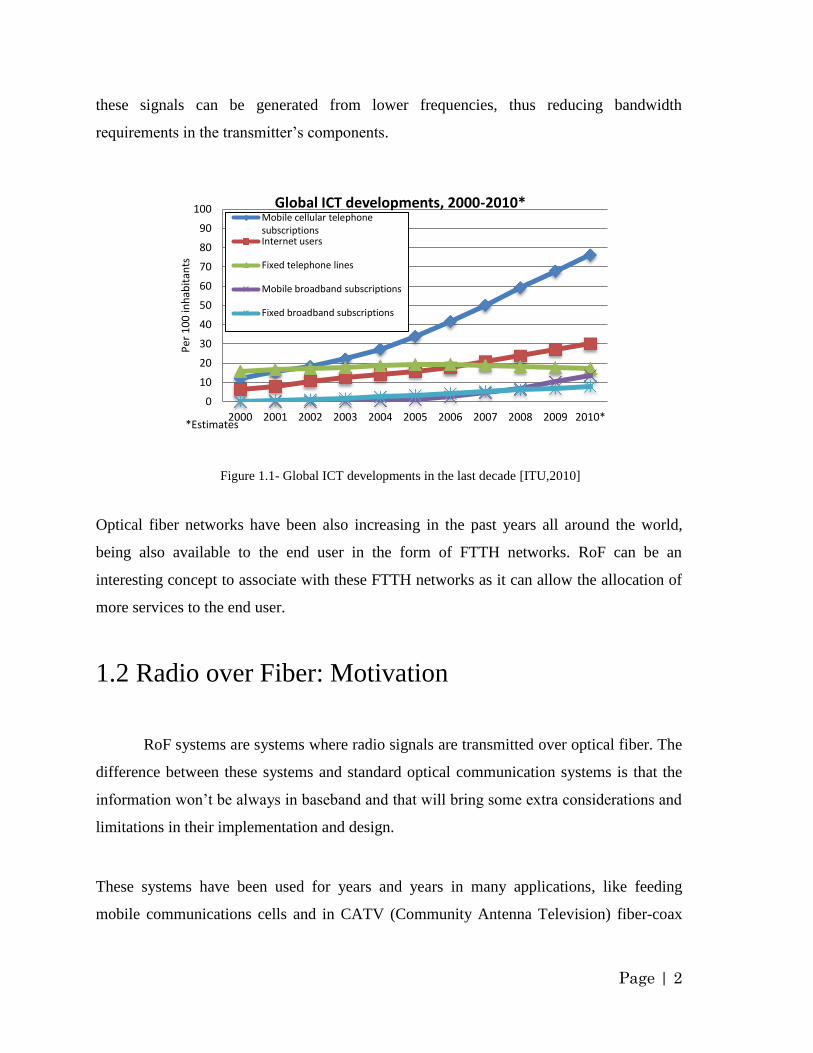
In the last years the evolution of wireless networks has been a
constant in telecommunications. The number of users subscribing to wireless technology is
increasing considerably since the last decade (see fig.1.1) allowing the fast growth of these
systems. This evolution has been possible because of the creation of many wireless
standards, that are available to the end user, like 2G and 3G mobile networks, WiFi
(Wireless LAN - IEEE 802.11), WiMax (IEEE 802.16), Terrestrial Digital TV broadcast
(DVB-T, DMB-T, ISDB-T), etc.
There are also many systems that may be deployed across the world and be easily
accessible to the end user in the next years, like the LTE/LTE Advanced 4G mobile
networks, UWB (Wireless PAN), 60 GHz WLAN. Wireless systems will require more
bandwidth and capacity in order to deliver more services, higher carrier frequencies and
high number of base stations (micro and pico-cells) that may increase the importance of
Radio over Fiber (RoF) technology. The generation of the radio signals in the optical
domain is also an important characteristic that may be explored in RoF systems, especially
when dealing with radio signals with high frequency carriers in the mm-wave band, as
Page | 2
these signals can be generated from lower frequencies, thus reducing bandwidth
requirements in the transmitter‟s components.
Figure 1.1- Global ICT developments in the last decade [ITU,2010]
Optical fiber networks have been also increasing in the past years all around the world,
being also available to the end user in the form of FTTH networks. RoF can be an
interesting concept to associate with these FTTH networks as it can allow the allocation of
more services to the end user.
1.2 Radio over Fiber: Motivation
RoF systems are systems where radio signals are transmitted over optical fiber. The
difference between these systems and standard optical communication systems is that the
information won‟t be always in baseband and that will bring some extra considerations and
limitations in their implementation and design.
These systems have been used for years and years in many applications, like feeding
mobile communications cells and in CATV (Community Antenna Television) fiber-coax
0
10
20
30
40
50
60
70
80
90
100
2000 2001 2002 2003 2004 2005 2006 2007 2008 2009 2010*
Per
10
0 in
hab
itan
ts
Global ICT developments, 2000-2010* Mobile cellular telephonesubscriptionsInternet users
Fixed telephone lines
Mobile broadband subscriptions
Fixed broadband subscriptions
*Estimates
Page | 3
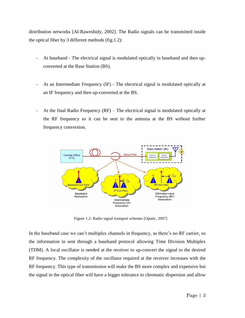
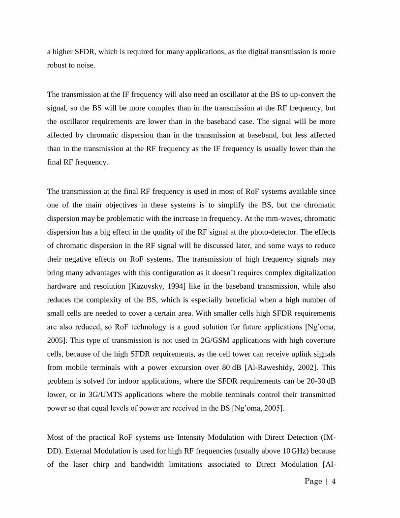
distribution networks [Al-Raweshidy, 2002]. The Radio signals can be transmitted inside
the optical fiber by 3 different methods (fig.1.2):
- At baseband - The electrical signal is modulated optically in baseband and then up-
converted at the Base Station (BS).
- At an Intermediate Frequency (IF) - The electrical signal is modulated optically at
an IF frequency and then up-converted at the BS.
- At the final Radio Frequency (RF) – The electrical signal is modulated optically at
the RF frequency so it can be sent to the antenna at the BS without further
frequency conversion.
Figure 1.2- Radio signal transport schemes [Opatic, 2007]
In the baseband case we can‟t multiplex channels in frequency, as there‟s no RF carrier, so
the information in sent through a baseband protocol allowing Time Division Multiplex
(TDM). A local oscillator is needed at the receiver to up-convert the signal to the desired
RF frequency. The complexity of the oscillator required at the receiver increases with the
RF frequency. This type of transmission will make the BS more complex and expensive but
the signal in the optical fiber will have a bigger tolerance to chromatic dispersion and allow
Page | 4
a higher SFDR, which is required for many applications, as the digital transmission is more
robust to noise.
The transmission at the IF frequency will also need an oscillator at the BS to up-convert the
signal, so the BS will be more complex than in the transmission at the RF frequency, but
the oscillator requirements are lower than in the baseband case. The signal will be more
affected by chromatic dispersion than in the transmission at baseband, but less affected
than in the transmission at the RF frequency as the IF frequency is usually lower than the
final RF frequency.
The transmission at the final RF frequency is used in most of RoF systems available since
one of the main objectives in these systems is to simplify the BS, but the chromatic
dispersion may be problematic with the increase in frequency. At the mm-waves, chromatic
dispersion has a big effect in the quality of the RF signal at the photo-detector. The effects
of chromatic dispersion in the RF signal will be discussed later, and some ways to reduce
their negative effects on RoF systems. The transmission of high frequency signals may
bring many advantages with this configuration as it doesn‟t requires complex digitalization
hardware and resolution [Kazovsky, 1994] like in the baseband transmission, while also
reduces the complexity of the BS, which is especially beneficial when a high number of
small cells are needed to cover a certain area. With smaller cells high SFDR requirements
are also reduced, so RoF technology is a good solution for future applications [Ng‟oma,
2005]. This type of transmission is not used in 2G/GSM applications with high coverture
cells, because of the high SFDR requirements, as the cell tower can receive uplink signals
from mobile terminals with a power excursion over 80 dB [Al-Raweshidy, 2002]. This
problem is solved for indoor applications, where the SFDR requirements can be 20-30 dB
lower, or in 3G/UMTS applications where the mobile terminals control their transmitted
power so that equal levels of power are received in the BS [Ng‟oma, 2005].
Most of the practical RoF systems use Intensity Modulation with Direct Detection (IM-
DD). External Modulation is used for high RF frequencies (usually above 10 GHz) because
of the laser chirp and bandwidth limitations associated to Direct Modulation [Al-
Page | 5
Raweshidy, 2002]. In the uplink, cheap lasers are always an important requirement. The
optical links are usually analog links (when baseband transmission is not used), so their
tolerance to noise is one of its biggest problems, making RIN noise a very important
parameter to take in consideration when designing a RoF system [Al-Raweshidy, 2002].
Next, we present some of the advantages of these systems:
Transparency to RF modulation, frequency, bitrate, protocols, etc. allowing multiple
services, in the same fiber, which can be multiplexed in a Sub-Carrier Multiplex
(SCM) scheme that has an easier implementation than TDM schemes [Kim,
2005][Al-Raweshidy, 2002] while it can also be combined with WDM [Agrawal,
2002]. This transparency brings a big advantage against coaxial links, in terms of
upgradeability and reconfiguration of the system, as because of the high attenuation
of the cable, thus, high Noise Figure (NF), will usually need a chain of regenerators,
which are dependent of the signal‟s characteristics.
Most of the usual operations like frequency allocation, modulation changes,
handover, upgrades, etc. can be centralized at the Central Office (CO). This also
allows a rapid response to variations in traffic demands. [Al-Raweshidy, 2002],
which makes it a good option for vehicle communications [Kim, 2005].
Reduction in the BS complexity, size, cost, maintenance expenses with an increase
in liability.
High bandwidth, low losses and electromagnetic interference immunity. The low
fiber loss that remains almost constant for a high bandwidth allows the use of high
distance links with minimal CNR (Carrier-to-Noise Ratio) reduction. Coaxial links
would require a high number of regenerator for a few kilometres of cable as the
signal degradation is superior because of its high attenuation that‟s also dependent
on the frequency, which increases the signal‟s distortion. In GSM links optical fiber
is the best choice in links with more than 100-200 m of length [Hunziker, 1998].
Page | 6
Efficient way to distribute signals with high carrier frequencies since high
attenuation in free space (that increase with the frequency) leads to Base Stations
(micro and pico-cells) with small coverage areas, thus requiring a high number of
BS to cover a considerable area, making the BS complexity reduction a priority.
Efficient way to cover areas where wireless access can be problematic like in
underground zones, tunnels and inside buildings with high capacity requirements
like airports, shopping centers, stadiums, etc. [Gonçalvez, 2010]
As we can see, RoF systems can be a cost effective approach for wireless applications,
being an important subject to be studied, especially because its importance will probably
increase with time, with the increase in bandwidth and carrier frequencies. The radio
signals can be transmitted over the optical fiber recurring to several types of optical
modulation, which will bring some advantages and limitations depending of the
characteristics of the system to be implemented. We intend to analyse the transmission of
radio signals using different kinds of optical modulation at the transmitter and assess their
performance.
1.3 Objectives and structure
The main objective of this work is to compare several types of optical modulation for
the transmission of OFDM radio signals, in the microwave and mm-wave frequency bands,
over fiber and assess their main advantages and limitations recurring to simulation tools.
We also intend to give a brief introduction to the importance of OFM (Optical Frequency
Multiplication) in future mm-band communications and solidify these concepts through
simulation. We will also study the transmission of several WPAN channels modelled
according to the standards ECMA-368 (MB-OFDM UWB) and ECMA-387 (60 GHz
WPAN). Finally we evaluate the performance of a simple system designed to deliver TV
programs to the end user, through fiber, recurring to digital video broadcast (DVB)
standards.
This document is divided in six chapters that are focused on Radio over Fiber systems.
Page | 7
The first chapter presents a brief introduction on RoF systems, their relevance in the last
years and possible future applications. The main objectives and motivation of this work are
also presented.
In Chapter 2 we describe some of the radio and video signals that can benefit from the use
of RoF systems. We will try to emulate the transmission of some of these signals over fiber
in later chapters recurring to the simulation tools available.
Chapter 3 consists of the study of several types of optical modulation in the transmission of
radio OFDM signals in the microwave (8 GHz) and mm-wave (60 GHz) frequency bands,
while also presents some of the advantages of OFM.
In Chapter 4 we evaluate the transmission of several WPAN radio channels, modelled
according to the WiMedia MB-OFDM UWB (ECMA-368) and 60 GHz WPAN (ECMA-
387).
Chapter 5 is focused on the distribution of digital TV (DVB) over optical fiber, in IM-DD
systems using external modulation.
Finally, in Chapter 6, the final conclusions of the whole work are presented, as well as
some proposed work for future research.
1.4 Main contributions
The main contributions of this work are:
Evaluation and comparison of Double Sideband (DSB), Double Sideband with
Carrier Suppression (DSB-CS) and Vestigial Sideband (VSB) optical modulation
types, through simulation, used in the transmission of OFDM radio channels in the
microwave and mm-wave frequency bands over different scenarios, considering
Standard Single Mode Fiber (SMF) and Non-Zero Dispersion-Shifted Fiber
(NZDSF);
Page | 8
Prove the efficiency of Optical Frequency Multiplication (OFM) in future
applications as a cost-effective alternative to the distribution of high frequency
radio-signals;
Comparison of several approaches to deliver WPAN signals, according to the
standards ECMA-368 (MB-OFDM UWB) and ECMA-387 (60 GHz WPAN), over
optical fiber;
Presentation and analysis of an external modulated RoF system designed for the
distribution of digital TV, according to the standards DVB-C and DVB-S, over
SSMF, near the 1550 nm wavelength. We also evaluate the advantages of biasing
the MZM near its transmission minimum in the distribution of DVB-C channels.
Additionally to the already mentioned contributions, the following paper was submitted to
the “Revista do Departamento de Electrónica e Telecomunicações da Universidade de
Aveiro”:
Paulo Andrade, Mário Lima, António Teixeira, “Distribution of OFDM radio signals
over optical fiber”, 2011.
The following paper will also be submitted soon:
Paulo Andrade, Mário Lima, António Teixeira, “Distribution of DVB-C channels
over an externally modulated optical link”, 2011.
Page | 9
Chapter 2. Characterization of radio and video signals
2.1 Introduction
This chapter will consist in the description of some of the RF signals
(carriers from 30 KHz to 300 GHz) that may benefit from RoF transmission. First we will
start by a brief introduction about single carrier and multi carrier systems and their impact
in wireless communications, and then proceed to the description of one of the most usual
and important modulations we can find in wireless standards, the multi carrier OFDM.
Then, we‟ll discuss some of the signals used in mobile communications and TV
distribution. We intend to describe these signals in order to use them in the next chapters
for simulation purposes, so knowing these signals is essential to build simulation models
that emulate their behaviour in the optical fiber.
2.2 Single and Multi carrier modulation
Single carrier modulation is the most primitive and simple method available. The
information sent to a certain target/user is associated with a single carrier frequency. This
method is not very effective for high bitrate wireless transmission in areas where Line-of-
Page | 10
Sight (LOS) can‟t be easily obtained, this is, where the signal received suffer multiple
reflections, so it will show up at the receiver at different times and may generate inter-
symbol interference (ISI) as the symbols reach the receiver at the wrong timeslots [Prasad,
2004]. Frequency selective fading will also affect certain zones where the signal can‟t get
to the receiver with enough power at the frequency used, as the reflectivity of the medium
is not constant with frequency. Because of the high frequency dependencies of the quality
of the signal, complex equalization filters are needed at the receiver [Prasad, 2004].
Multi-carrier modulation is very effective in these situations since the information is
divided in many narrowband sub-carriers at slow symbol rates, which allow the possibility
to use guard times higher than the max delay the signals can suffer from multipath.
Because the information is divided in many carriers the effects of frequency selective
fading won‟t affect all carriers, allowing the FEC (Forward Error Correction) combined
with frequency and/or time interleaving to improve the reception performance [Prasad,
2004]. Because of these advantages in rough propagation mediums, multi-carrier
modulation is used in most of the current wireless standards that allow high bitrates. The
technology is more complex than in single carrier modulation, but many advances in this
area has been happening in the last years reducing its implementation costs.
The most important multi-carrier modulation is Orthogonal Frequency Division Multiplex
(OFDM). We‟ll give a brief description about OFDM in the next section since it‟s one of
the most common modulations in wireless standards and we‟ll use OFDM signals for
simulation purposes in RoF systems in the next chapters.
2.3 Orthogonal Frequency Division Multiplex
(OFDM)
OFDM is a multi-carrier modulation method that consist in a parallel transmission
of many (usually thousands) low-rate substreams (obtained by the division of a high-rate
Page | 11
stream), where each one of those low-rate substreams are modulated by separate
subcarriers using QPSK or QAM in most cases. The separation between these narrowband
subcarriers is small. By selecting a set of orthogonal carrier frequencies, high spectral
efficiency is obtained because the spectra of the subcarriers overlap, while mutual influence
among the subcarriers can be avoided [Prasad, 2004].
OFDM is the modulation scheme of many wireless communications systems such as
WLAN (WiFi), WMAN (WiMAX), WPAN (MB-OFDM UWB), digital TV broadcasting
(DVB-T, T-DMB, ISDB-T, DVB-H), digital audio broadcasting (DAB) and mobile
systems (3GPP LTE). It‟s also used in cable transmission standards like ADSL
(Asymmetric Digital Subscriber Line) [Proakis, 2005].
Some of the advantages of OFDM are robustness to multipath effects like frequency and
location selective fading and ISI, reduced equalization complexity, efficient
implementation using Fast-Fourier Transform (FFT) and high spectral efficiency. It also
has disadvantages like high Peak-to-Average-Power Ratio (PAPR) and frequency and
phase sensitivity [Prasad, 2004].
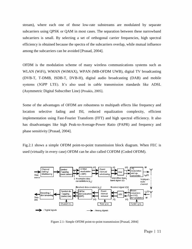
Fig.2.1 shows a simple OFDM point-to-point transmission block diagram. When FEC is
used (virtually in every case) OFDM can be also called COFDM (Coded OFDM).
Figure 2.1- Simple OFDM point-to-point transmission [Prasad, 2004]
Page | 12
The multiple subcarriers are generated using the Discrete Fourier Transform (DCT) and
Inverse DCT (IDCT). The number of subcarriers N is usually a number power of two so the
FFT and IFFT are used instead of DCT and IDCT, improving efficiency. OFDMA
(Orthogonal Frequency Division Multiple Access) is implemented allocating a limited
number of subcarriers to each user [Prasad, 2004].
2.4 Mobile phone signals
Mobile phone networks use a cellular structure where each BS corresponds to one
cell, that can be denominated as macro, micro, pico or femto cell depending to its coverage
area. Macro cells when the cover area is over 2 km wide, micro when it‟s less than 2 km,
pico when it‟s less than 200 meters and femto around 10 m.
The backhaul for these systems is usually done by microwave, copper or fiber. With the
evolution in mobile phone systems like the growth of 3G and the introduction of LTE and
soon 4G, bandwidth requirements will be too much for copper links, so the two methods
that will prevail will be microwave and optical fiber.
2.4.1 GSM (2G)
GSM is the primary standard for 2G digital mobile phone communications
replacing first generation analog systems and it is the mobile system with more subscribers
worldwide (see fig.2.2). The most common GSM system are the GSM900, that uses the
935-960 MHz band for downlink and the 890-915 MHz band for uplink and, that is
deployed in Europe and the GSM at 1800 MHz that uses 1710-1785 MHz for uplink and
1805-1880 MHz for downlink [Schiller, 2003]. In other countries where these bands were
already occupied GSM is operated at 850 MHz or 1900 MHz (1850-1910 MHz uplink and
1930-1990 MHz downlink) like in the US or Canada. There‟re also GSM systems operating
at 400 or 450 MHz.
Page | 13
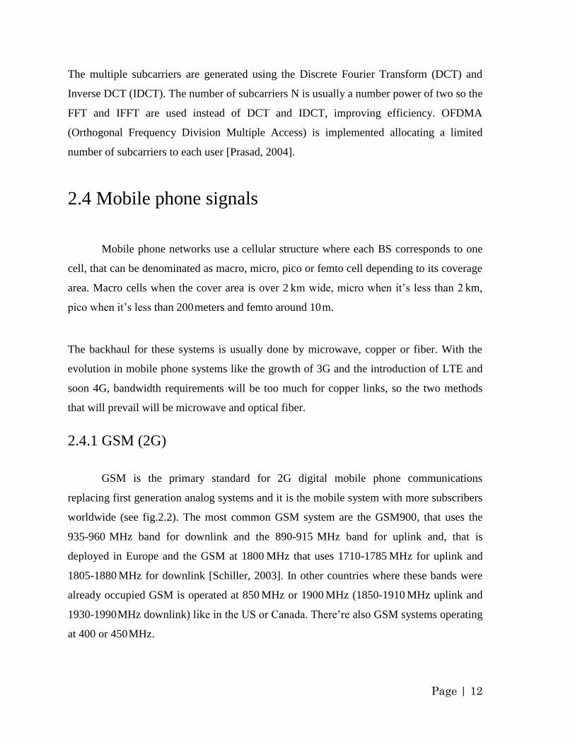
Figure 2.2- Evolution of 2G and 3G subscribers [ITU, 2010]
Uplink and Downlink are separated by Frequency Division Duplexing (FDD) and use
TDMA in combination with FDMA as multiple access method. In GSM 900, 124 channels,
each 200 kHz wide, are used for FDMA, whereas GSM 1800 uses, 374 channels [Schiller,
2003]. Each channel data frame is divided into 8 time slots or TDM channels. To counter
frequency selective fading, frequency hopping is used, changing the carrier of a frame in a
determined hoping sequence [Schiller, 2003].
Gaussian minimum shift keying (GMSK) is the modulation used in GSM allowing data
rates of 9.6 kbps or other values according to the FEC used. Transmission in GSM is half-
duplex.
2.4.2 UMTS (3G)
UMTS is the main standard of 3G mobile phone systems and its number of
subscribers is increasing in the last years (see fig.2.2). UMTS allows much higher bitrates
than GSM (can reach 2 Mbps) so it can offer an increased number of services like mobile
TV and Video calling. W-CDMA (Wideband-CDMA) is the most common form of UMTS,
but there‟re many variants. It uses Code Division Multiple Access (CDMA), as an access
method, assigning different codes to different users as the bandwidth is shared between
them and Quadrature Phase Shift Keying (QPSK) as modulation format [Schiller, 2003].
Page | 14
The bandwidth allocated to uplink and downlink is, in most cases, 60 MHz, centered at 1.95
GHz and 2.14 GHz [ETSI, 2008]. Both frequency bands are divided into 12 channels with a
bandwidth of 3.84 MHz, and a 5 MHz separation between channels [ETSI, 2008].
2.4.3 3GGP LTE
This standard uses OFDMA with QPSK, 16QAM or 64QAM modulation in
bandwidths of 1.4, 3, 5, 10, 15 and 20 MHz and 15 kHz channel spacing [3GGP, 2011]. It
can achieve 100 Mbps at the downlink and 50 Mbps at the uplink at 20 MHz channel
bandwidths. It is sometimes marketed as a 4G mobile technology, though it‟s still
considered a 3G standard. The 3GGP (3rd Generation Partnership Project) formally
submitted to ITU-T the LTE Advanced as a candidate 4G system in 2009 and it‟s expected
to be finalized in 2011 [3GGP, 2011].
2.5 TV distribution signals
Since the beginning of analog video broadcast, that this technology became relevant
and familiar in the whole world. In the last 2 decades digital TV started to rise in many
countries replacing analog TV, fact that is bonded to happen in most countries that still use
the analog form of video broadcast. Analog and digital video signals are usually distributed
to the users by cable (coaxial or fiber), satellite or by terrestrial wireless with the use of
rooftop antennas. There‟re also others methods that start to be part of the everyday
language like the IPTV and Mobile TV [Fischer, 2008].
Video broadcasting can be considered a broadband technology since the channels used in
analog and digital TV range from 6 to 8 MHz for cable and terrestrial transmission and 36
MHz for satellite transmission. These channels are so wide that is very common to allow
high speed internet to the end user in one video channel.
Page | 15
2.5.1 Analog TV
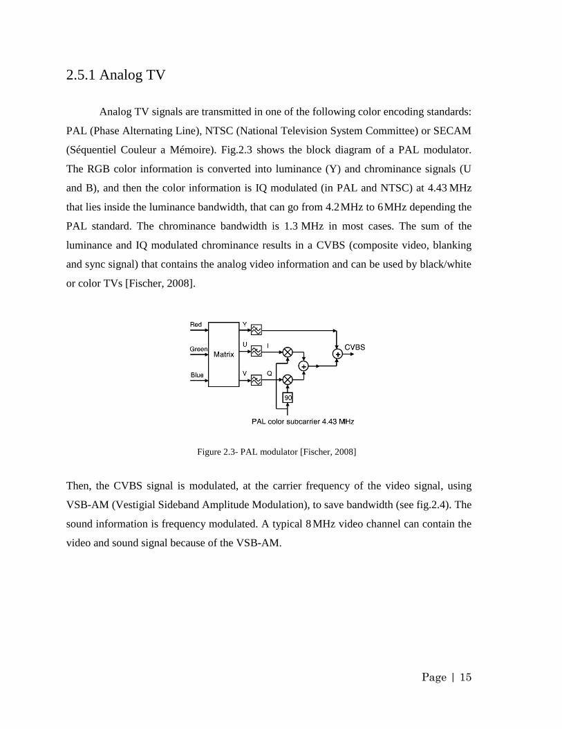
Analog TV signals are transmitted in one of the following color encoding standards:
PAL (Phase Alternating Line), NTSC (National Television System Committee) or SECAM
(Séquentiel Couleur a Mémoire). Fig.2.3 shows the block diagram of a PAL modulator.
The RGB color information is converted into luminance (Y) and chrominance signals (U
and B), and then the color information is IQ modulated (in PAL and NTSC) at 4.43 MHz
that lies inside the luminance bandwidth, that can go from 4.2 MHz to 6 MHz depending the
PAL standard. The chrominance bandwidth is 1.3 MHz in most cases. The sum of the
luminance and IQ modulated chrominance results in a CVBS (composite video, blanking
and sync signal) that contains the analog video information and can be used by black/white
or color TVs [Fischer, 2008].
Figure 2.3- PAL modulator [Fischer, 2008]
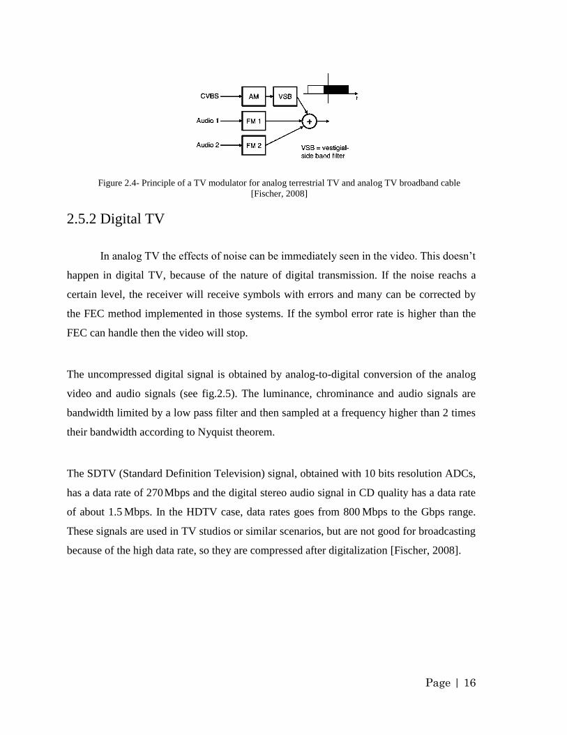
Then, the CVBS signal is modulated, at the carrier frequency of the video signal, using
VSB-AM (Vestigial Sideband Amplitude Modulation), to save bandwidth (see fig.2.4). The
sound information is frequency modulated. A typical 8 MHz video channel can contain the
video and sound signal because of the VSB-AM.
Page | 16
Figure 2.4- Principle of a TV modulator for analog terrestrial TV and analog TV broadband cable
[Fischer, 2008]
2.5.2 Digital TV
In analog TV the effects of noise can be immediately seen in the video. This doesn‟t
happen in digital TV, because of the nature of digital transmission. If the noise reachs a
certain level, the receiver will receive symbols with errors and many can be corrected by
the FEC method implemented in those systems. If the symbol error rate is higher than the
FEC can handle then the video will stop.
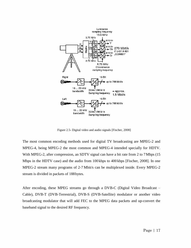
The uncompressed digital signal is obtained by analog-to-digital conversion of the analog
video and audio signals (see fig.2.5). The luminance, chrominance and audio signals are
bandwidth limited by a low pass filter and then sampled at a frequency higher than 2 times
their bandwidth according to Nyquist theorem.
The SDTV (Standard Definition Television) signal, obtained with 10 bits resolution ADCs,
has a data rate of 270 Mbps and the digital stereo audio signal in CD quality has a data rate
of about 1.5 Mbps. In the HDTV case, data rates goes from 800 Mbps to the Gbps range.
These signals are used in TV studios or similar scenarios, but are not good for broadcasting
because of the high data rate, so they are compressed after digitalization [Fischer, 2008].
Page | 17
Figure 2.5- Digital video and audio signals [Fischer, 2008]
The most common encoding methods used for digital TV broadcasting are MPEG-2 and
MPEG-4, being MPEG-2 the most common and MPEG-4 intended specially for HDTV.
With MPEG-2, after compression, an SDTV signal can have a bit rate from 2 to 7 Mbps (15
Mbps in the HDTV case) and the audio from 100 kbps to 400 kbps [Fischer, 2008]. In one
MPEG-2 stream many programs of 2-7 Mbit/s can be multiplexed inside. Every MPEG-2
stream is divided in packets of 188 bytes.
After encoding, these MPEG streams go through a DVB-C (Digital Video Broadcast –
Cable), DVB-T (DVB-Terrestrial), DVB-S (DVB-Satellite) modulator or another video
broadcasting modulator that will add FEC to the MPEG data packets and up-convert the
baseband signal to the desired RF frequency.
Page | 18
In digital TV broadcasting the required CNR at the receiver is lower than in analog TV.
The national Association of Broadcasters requires a CNR of 46 dB on standard NTSC video
channels (measured at the TV) [Woodward, 1999]. In digital TV this value depends on the
modulation format of the broadcast standard used, being lower than 10-20 dB in more
robust systems like in satellite or terrestrial transmission, or around 30 dB for fiber
transmission (using 256QAM). A single digital TV channel can deliver many TV
programs, with better quality, less sensitivity to noise, and requiring lower CNR than a
single analog TV channel, that can only transmit one TV program and require high linearity
components [Agrawal, 2002].
2.5.2.1 DVB-S and DVB-S2
Reception of TV via satellite has been very common in many countries as the price
of a simple satellite receiver system is not very high and many TV channels are available
for free in the analog or digital form [Fischer, 2008].
Quadrature Phase Shift Keying (QPSK) is the modulation format used in DVB-S, as
satellite transmissions need a robust modulation format capable to handle intense noise and
non-linearity. The active element in a satellite transponder is the TWA (Travelling Wave
Amplifier) that has a high non-linear response, so amplitude modulation is not the right
choice to these applications. In satellite analog TV distribution frequency modulation is
used.
A DBS (Direct-Broadcast Satellite) system uses channels with 26 MHz to 36 MHz
bandwidth in most cases, uplink in the 14-19 GHz band and the downlink is 11-13 GHz.
The symbol rate is in most cases 27.5 MS/s (55 Mbps with QPSK) in order to fit the
bandwidth available [Fischer, 2008].
The FEC in DVB-S must be strong enough to handle many errors, so Reed-Solomon block
code (204,188) is used along with a convolutional code to protect each MPEG-2 188bytes
packet. FEC will add redundancy so the effective bit rate available for satellite transmission
Page | 19
will be reduced and dependent on the code rate used in both error correction methods
(normally only the convolutional error correction code rate is changed). The information is
interleaved before the FEC (that can only correct a limited number of errors in a packet) in
order to be capable to handle burst of errors, spreading them so may be corrected.
With a ¾ code rate in the convolutional error correction method we obtain an effective bit
rate of 38.01 Mbps [Fischer, 2008]. After mapping the symbols of the QPSK constellation,
a „roll-off‟ filter is applied with a roll-off factor of 0.35 and then modulated, up-converted
to the microwave uplink frequency, amplified and fed to the antenna satellite. At the
receiver the signal goes through 2 IF stages, before the MPEG stream is decoded.
DVB-S2 is based on DVB-S and DSNG (Digital Satellite News Gathering), a satellite
communication standard for mobile units, and it‟s expected to fully overcome DVB-S in
the future as it‟s more flexible and efficient being also compatible with DVB-S. It allows
QPSK, 8PSK, 16APSK (Amplitude Phase Shift Keying) and 36APSK, being the first 2
usually used in broadcasting. The standard is compatible with data streams different than
MPEG-2, and allows Adaptive Coding and Modulation (ACM) so code and modulation can
adapt to the reception conditions, increasing error correction and using robust modulation
schemes when the signals strength is too low.
DVB-S2 uses a very powerful FEC system, that‟s a concatenation of BCH (Bose-
Chaudhuri-Hcquengham) with LDPC (Low Density Parity Check) inner coding [DVB,
2011].
2.5.2.2 DVB-C
Analog and digital TV distribution by cable is very common in most countries
allowing a high number of TV channels and also high speed internet access. Transmission
of digital TV via cable (coaxial or fiber) is done using the DVB-C standard. As in this case,
the channel has much better transmission characteristics, than the one in satellite
communications, higher order modulations can be used. When the transmission is done via
Page | 20
coaxial cable the modulation used to deliver the MPEG-2 streams is usually 64QAM and
256QAM for optical fiber. Frequently there‟s also a return channel link in the frequency
band below about 65 MHz [Fischer, 2008].
Because of the high order modulation formats and FEC used, in any generic analog TV
channel of 8 MHz, a high bitrate can be delivered. In this case only Reed-Solomon
(188,204) is used as FEC, as the transmission channel is not so demanding like in satellite
communications. The DVB-C standard modulation formats are 16QAM, 32QAM, 64QAM,
128QAM and 256QAM with a 0.15 roll-off factor.
In North America is used the ITU-T J83B standard while Japan use the ITU-T J83C
standard for cable digital TV transmissions having both some similarities and differences to
DVB-C [Fischer, 2008].
2.5.2.3 DVB-T
DVB-T uses COFDM to modulate the MPEG streams allowing hierarquical
modulation in order to transmit the same programs with different FEC, data rates and video
quality. The high priority data stream is modulated at QPSK with better error correction
while the low priority data stream uses higher order modulation like 16QAM or 64QAM
with higher code rates and video quality. The data stream is chosen according to the
reception conditions.
DVB-T can have channels bandwidths of 6, 7 or 8 MHz operating at the 2K (2046
subcarriers) or 8K (8192 subcarriers) modes. The 2k mode has a higher subcarrier spacing
of 4 kHz (1 kKz in the 8K mode) but shorter symbol period, being more susceptible to time
delays at the receiver but less affected by frequency shifts (Doppler Effect). FEC used in
DVB-T is similar to the one used in DVB-S [Fischer, 2008].
In North America ATSC (Advanced Television Systems Committee) is the terrestrial video
broadcasting method adopted, using in this case 8VSB (8 level VSB). The ISDB-T
Page | 21
(Integrated Services Digital Broadcasting - Terrestrial) standard is used in Japan and Brasil
and the MPEG streams are modulated by COFDM as in DVB-T [Fischer, 2008].
2.6 Wireless Personal Area Networks (WPAN) signals
WPAN systems are used to communicate at short distances of a few meters using
low-power consumption and small size devices. Some of the most common WPAN
systems are for example Bluetooth, ZigBee and the Wireless USB that is based on the
WiMedia MB-OFDM technology.
2.6.1 WiMedia MB-OFDM UWB (ECMA-368)
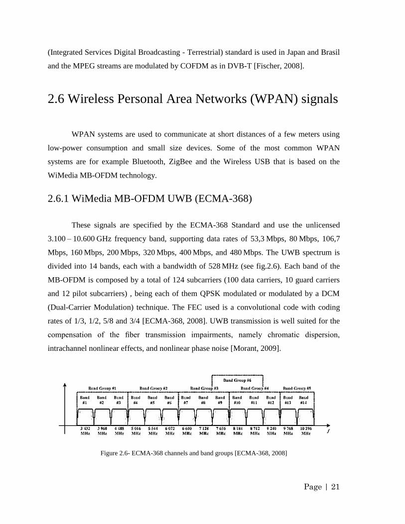
These signals are specified by the ECMA-368 Standard and use the unlicensed
3.100 – 10.600 GHz frequency band, supporting data rates of 53,3 Mbps, 80 Mbps, 106,7
Mbps, 160 Mbps, 200 Mbps, 320 Mbps, 400 Mbps, and 480 Mbps. The UWB spectrum is
divided into 14 bands, each with a bandwidth of 528 MHz (see fig.2.6). Each band of the
MB-OFDM is composed by a total of 124 subcarriers (100 data carriers, 10 guard carriers
and 12 pilot subcarriers) , being each of them QPSK modulated or modulated by a DCM
(Dual-Carrier Modulation) technique. The FEC used is a convolutional code with coding
rates of 1/3, 1/2, 5/8 and 3/4 [ECMA-368, 2008]. UWB transmission is well suited for the
compensation of the fiber transmission impairments, namely chromatic dispersion,
intrachannel nonlinear effects, and nonlinear phase noise [Morant, 2009].
Figure 2.6- ECMA-368 channels and band groups [ECMA-368, 2008]
Page | 22
2.6.2 60 GHz WPAN (ECMA-387)
Millimeter-wave wireless communications are an attractive solution for high-speed
data transmission because of the spectrum availability at these frequency bands [Mohamed,
2009]. The unlicensed bands at 60 GHz can be used for high bitrate short-range
communications (short distances due to the oxygen absorption peak) in WPAN networks
with low-power consumption and small size devices. Some of the applications at these
frequency bands can be for example uncompressed High-Definition Video streaming and
high speed file transmission between handheld devices [ECMA-387, 2010].
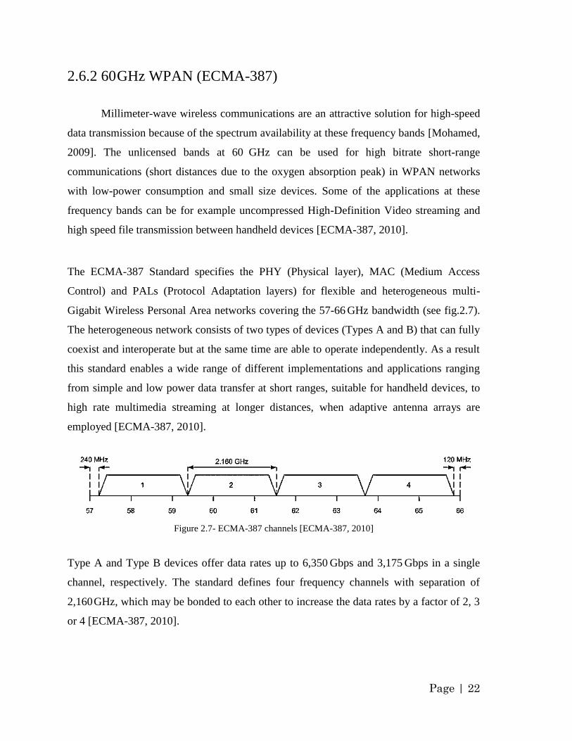
The ECMA-387 Standard specifies the PHY (Physical layer), MAC (Medium Access
Control) and PALs (Protocol Adaptation layers) for flexible and heterogeneous multi-
Gigabit Wireless Personal Area networks covering the 57-66 GHz bandwidth (see fig.2.7).
The heterogeneous network consists of two types of devices (Types A and B) that can fully
coexist and interoperate but at the same time are able to operate independently. As a result
this standard enables a wide range of different implementations and applications ranging
from simple and low power data transfer at short ranges, suitable for handheld devices, to
high rate multimedia streaming at longer distances, when adaptive antenna arrays are
employed [ECMA-387, 2010].
Figure 2.7- ECMA-387 channels [ECMA-387, 2010]
Type A and Type B devices offer data rates up to 6,350 Gbps and 3,175 Gbps in a single
channel, respectively. The standard defines four frequency channels with separation of
2,160 GHz, which may be bonded to each other to increase the data rates by a factor of 2, 3
or 4 [ECMA-387, 2010].
Page | 23
Chapter 3. Distribution of OFDM radio signals over
optical fiber
3.1 Introduction
In this chapter we will present a few types of system configurations
to deliver RF signals over optical fiber and assess its performance using the software
VPITransmissionMaker™. We will start by describing the configurations used in this
chapter while comparing their performance using the transmission of OFDM signals at 8
GHz and 60 GHz. We used these frequency bands as they fit inside the bands used in the
standards ECMA-368 Multiband OFDM UWB (3.1 - 10.6 GHz) and the ECMA-387 (57 - 64
GHz), used in WPAN applications, which we will study in the next chapter.
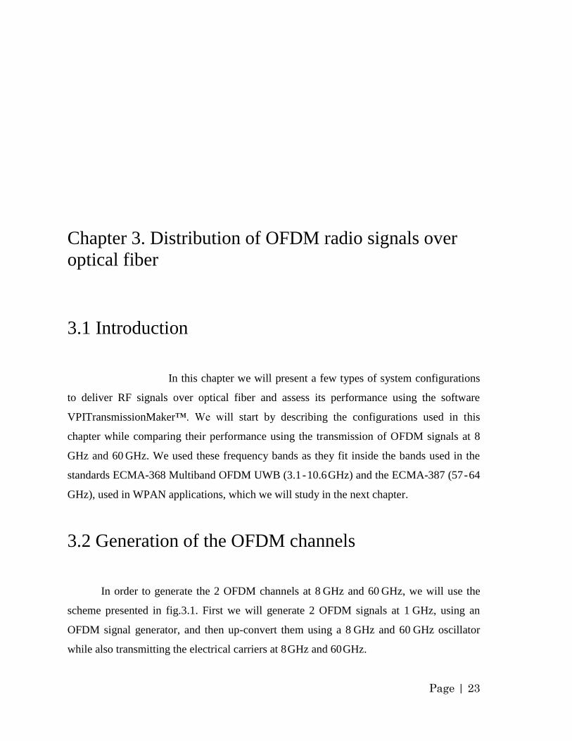
3.2 Generation of the OFDM channels
In order to generate the 2 OFDM channels at 8 GHz and 60 GHz, we will use the
scheme presented in fig.3.1. First we will generate 2 OFDM signals at 1 GHz, using an
OFDM signal generator, and then up-convert them using a 8 GHz and 60 GHz oscillator
while also transmitting the electrical carriers at 8 GHz and 60 GHz.
Page | 24
Figure 3.1- Generation of OFDM channels using VPITransmissionMaker™
Using that that setup at the transmitter, we intend to down-convert the signals to 1 GHz, at
the receiver, and evaluate their EVM recurring to an OFDM signal analyser. In this chapter,
we chose this transmission scheme in order to enable the comparison of the configurations
studied below, since there are some limitations in the simulator modules. The OFDM signal
generator and analyser, require the same frequency in order to operate correctly, so it
wouldn‟t be possible to use them in the DSB-CS configuration, without the use of an
intermediate frequency, because as we will see in 3.5, the carrier suppression generates
frequency duplication at the optical-to-electrical conversion.
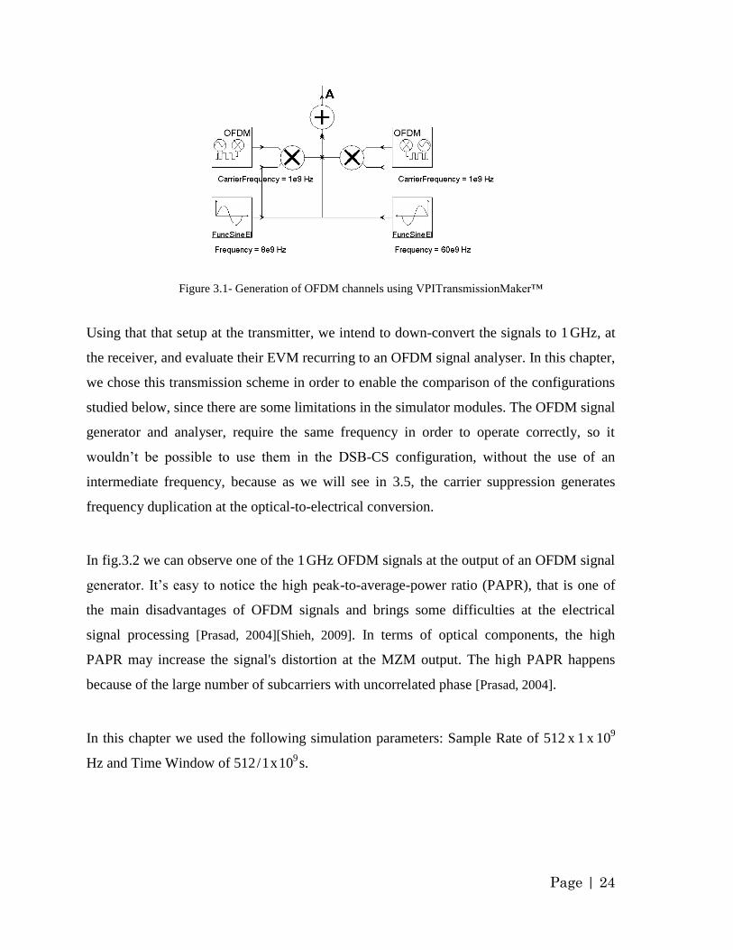
In fig.3.2 we can observe one of the 1 GHz OFDM signals at the output of an OFDM signal
generator. It‟s easy to notice the high peak-to-average-power ratio (PAPR), that is one of
the main disadvantages of OFDM signals and brings some difficulties at the electrical
signal processing [Prasad, 2004][Shieh, 2009]. In terms of optical components, the high
PAPR may increase the signal's distortion at the MZM output. The high PAPR happens
because of the large number of subcarriers with uncorrelated phase [Prasad, 2004].
In this chapter we used the following simulation parameters: Sample Rate of 512 x 1 x 109
Hz and Time Window of 512 / 1 x 10⁹
s.
Page | 25
Figure 3.2- OFDM signal at 1 GHz
The OFDM signals, generated at 1 GHz, have a bit rate (R) of 1 Gbps, 16 subcarriers
modulated 16QAM (N = 4 bits/symbol) and a roll-off factor (r) of 0.18. Each one of these
OFDM signals has a bandwidth (B) of:
( )
( ) (3.1)
The bandwidth is determined by the OFDM signal generator, being only dependent on
those 3 parameters.
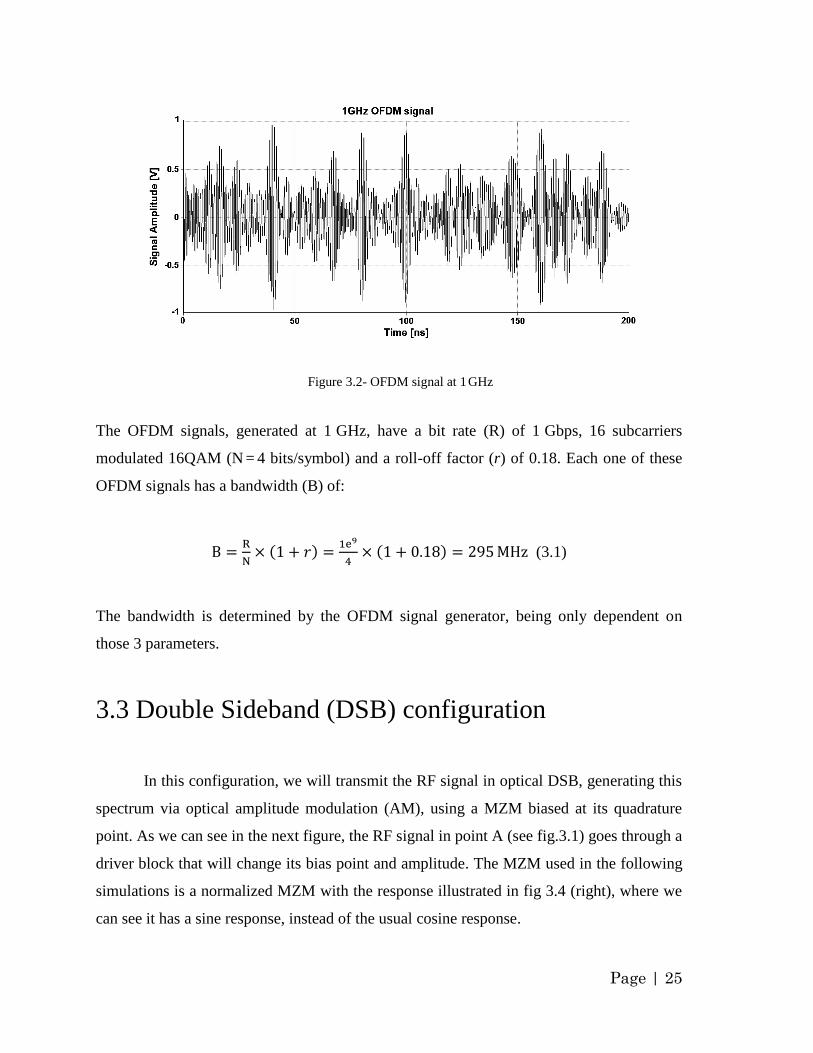
3.3 Double Sideband (DSB) configuration
In this configuration, we will transmit the RF signal in optical DSB, generating this
spectrum via optical amplitude modulation (AM), using a MZM biased at its quadrature
point. As we can see in the next figure, the RF signal in point A (see fig.3.1) goes through a
driver block that will change its bias point and amplitude. The MZM used in the following
simulations is a normalized MZM with the response illustrated in fig 3.4 (right), where we
can see it has a sine response, instead of the usual cosine response.
Page | 26
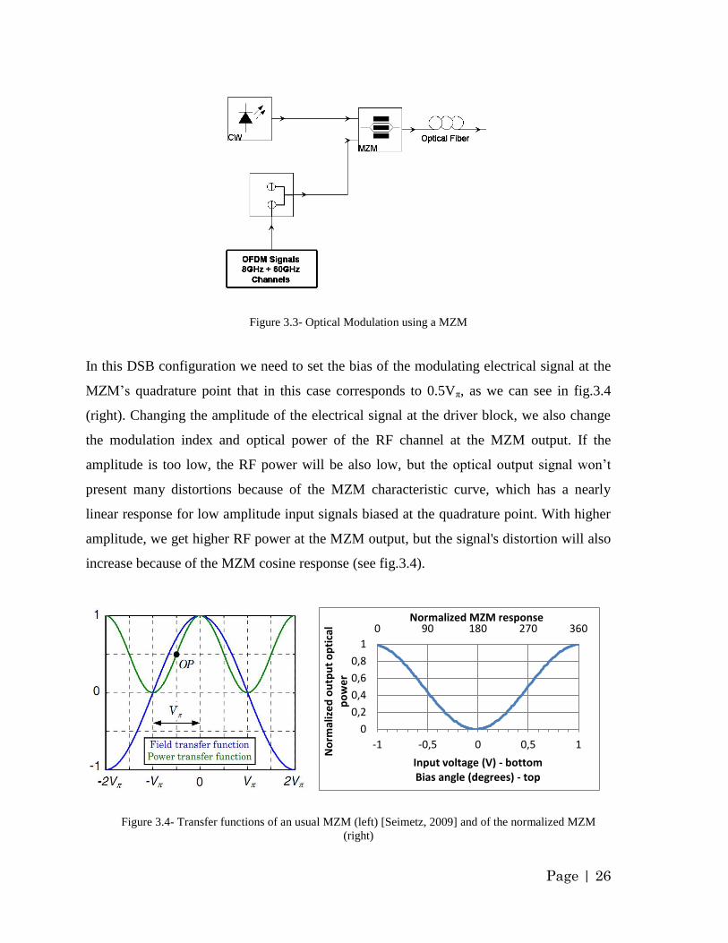
Figure 3.3- Optical Modulation using a MZM
In this DSB configuration we need to set the bias of the modulating electrical signal at the
MZM‟s quadrature point that in this case corresponds to 0.5Vπ, as we can see in fig.3.4
(right). Changing the amplitude of the electrical signal at the driver block, we also change
the modulation index and optical power of the RF channel at the MZM output. If the
amplitude is too low, the RF power will be also low, but the optical output signal won‟t
present many distortions because of the MZM characteristic curve, which has a nearly
linear response for low amplitude input signals biased at the quadrature point. With higher
amplitude, we get higher RF power at the MZM output, but the signal's distortion will also
increase because of the MZM cosine response (see fig.3.4).
Figure 3.4- Transfer functions of an usual MZM (left) [Seimetz, 2009] and of the normalized MZM
(right)
0 90 180 270 360
0
0,2
0,4
0,6
0,8
1
-1 -0,5 0 0,5 1
No
rmal
ize
d o
utp
ut
op
tica
l p
ow
er
Input voltage (V) - bottom Bias angle (degrees) - top
Normalized MZM response
Page | 27
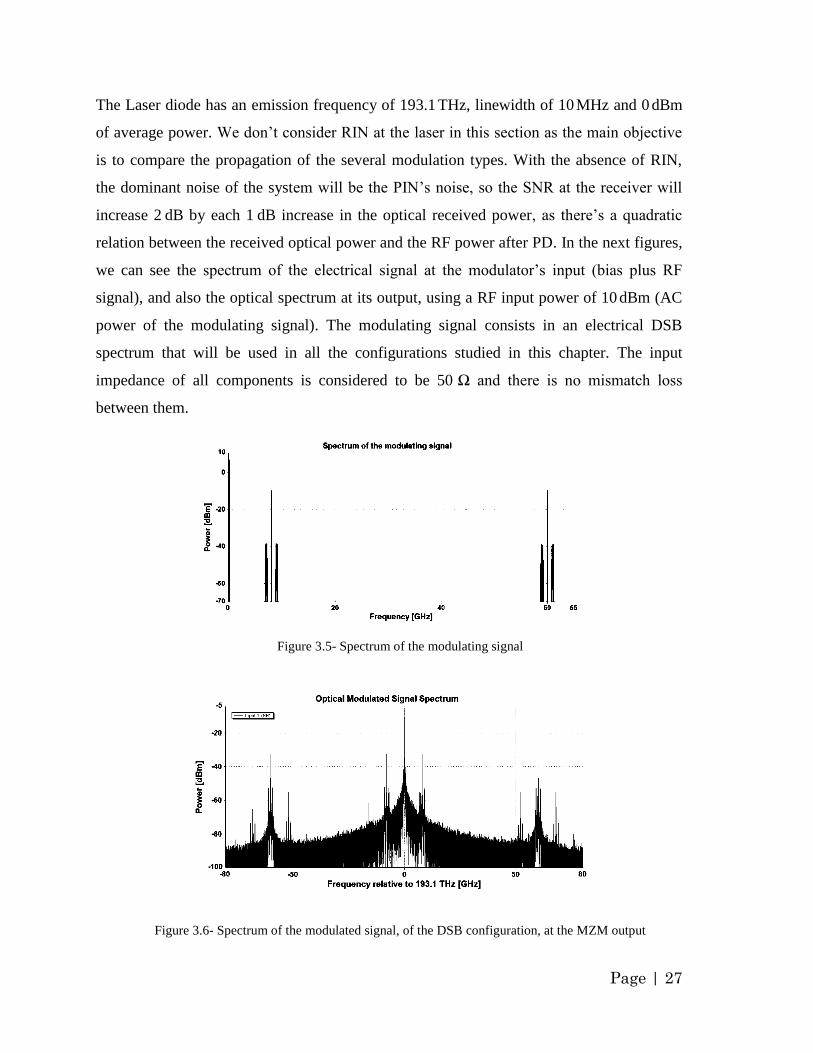
The Laser diode has an emission frequency of 193.1 THz, linewidth of 10 MHz and 0 dBm
of average power. We don‟t consider RIN at the laser in this section as the main objective
is to compare the propagation of the several modulation types. With the absence of RIN,
the dominant noise of the system will be the PIN‟s noise, so the SNR at the receiver will
increase 2 dB by each 1 dB increase in the optical received power, as there‟s a quadratic
relation between the received optical power and the RF power after PD. In the next figures,
we can see the spectrum of the electrical signal at the modulator‟s input (bias plus RF
signal), and also the optical spectrum at its output, using a RF input power of 10 dBm (AC
power of the modulating signal). The modulating signal consists in an electrical DSB
spectrum that will be used in all the configurations studied in this chapter. The input
impedance of all components is considered to be 50 Ω and there is no mismatch loss
between them.
Figure 3.5- Spectrum of the modulating signal
Figure 3.6- Spectrum of the modulated signal, of the DSB configuration, at the MZM output
Page | 28
We can see the DSB spectrum in fig.3.6, which is composed by the optical carrier and 2
sidebands that carry the OFDM channels at 8 GHz (ω1) and 60 GHz (ω2). We can also see a
few of the second-order distortion components, like at 16 GHz (2.ω1), and also at 52 GHz
(ω2 - ω1) and 68 GHz (ω2 + ω1). These terms appear because of the non-linear response of
the MZM and can be reduced by decreasing the amplitude of the modulating RF signal. A
particular detail that we can also observe on the optical spectrum, at the MZM output, is
that the second-order components that can be clearly seen are only the ones with products
from the electrical carriers, as the carriers are transmitted with more power than the OFDM
channels. The power contained in one of the electrical sidebands is nearly 13 dB lower than
the power of one of the electrical carriers. We could attenuate the electrical carriers in order
to allow higher RF power on the OFDM channels, as the modulating signal is composed by
the sum of the channels at 8 GHz and 60 GHz with the electrical carriers, while at the same
time the RF power at the MZM input is limited by the distortion of the modulators
nonlinear response. We will keep the modulating signal with those characteristics, because
it will allow us to perform a better comparison between the different configurations. Our
DSB-CS configuration, for instance, needs higher power in the electrical carriers, in order
to obtain a good reception at the PD, as we will see in section 3.5.
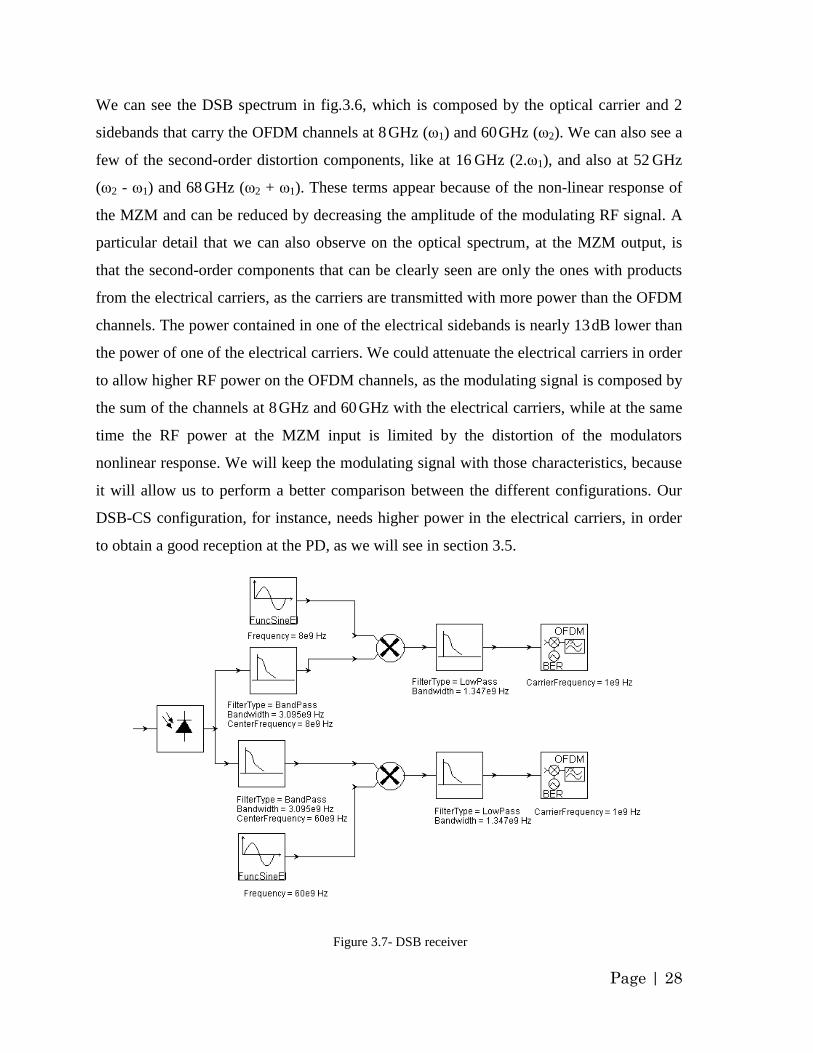
Figure 3.7- DSB receiver
Page | 29
The optical fiber used is a SMF with 0.2 dB/km of attenuation and 16 ps/nm/km of
dispersion at the laser's wavelength with a 0.08 ps/nm2/km slope. The receiver is presented
in fig.3.7. The band-pass filters after the PD are used for measuring purposes and can be
neglected in a real system.
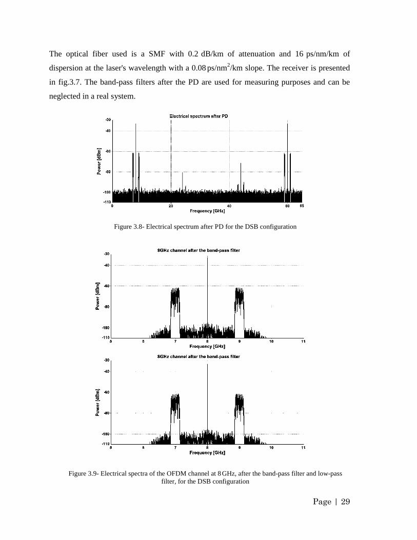
Figure 3.8- Electrical spectrum after PD for the DSB configuration
Figure 3.9- Electrical spectra of the OFDM channel at 8 GHz, after the band-pass filter and low-pass
filter, for the DSB configuration
Page | 30
The photodiode used in all the simulations was a PIN with 1 A/W responsivity and 1x10-11
A/√ of thermal noise and without bandwidth limitations. Both channels pass through a
bandpass filter, with enough bandwidth to cover the electrical DSB spectrum centered at 8
GHz and 60 GHz. Then, the signals are down-converted to the IF frequency of 1 GHz, low-
pass filtered, and finally, 2 signal analyzers measure the EVM of the OFDM signal at 1
GHz. The optimal phase of the local oscillators at 8 GHz and 60 GHz are determined by
simulation at the different fiber lengths studied. Fig.3.8 and 3.9, present the spectra after
the optical-to-electrical conversion and after the electrical filters (for the channel at 8 GHz),
for a back-to-back (B2B) setup.
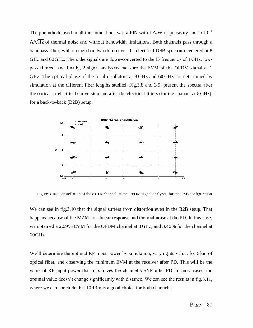
Figure 3.10- Constellation of the 8 GHz channel, at the OFDM signal analyzer, for the DSB configuration
We can see in fig.3.10 that the signal suffers from distortion even in the B2B setup. That
happens because of the MZM non-linear response and thermal noise at the PD. In this case,
we obtained a 2.69 % EVM for the OFDM channel at 8 GHz, and 3.46 % for the channel at
60 GHz.
We‟ll determine the optimal RF input power by simulation, varying its value, for 5 km of
optical fiber, and observing the minimum EVM at the receiver after PD. This will be the
value of RF input power that maximizes the channel‟s SNR after PD. In most cases, the
optimal value doesn‟t change significantly with distance. We can see the results in fig.3.11,
where we can conclude that 10 dBm is a good choice for both channels.
Page | 31
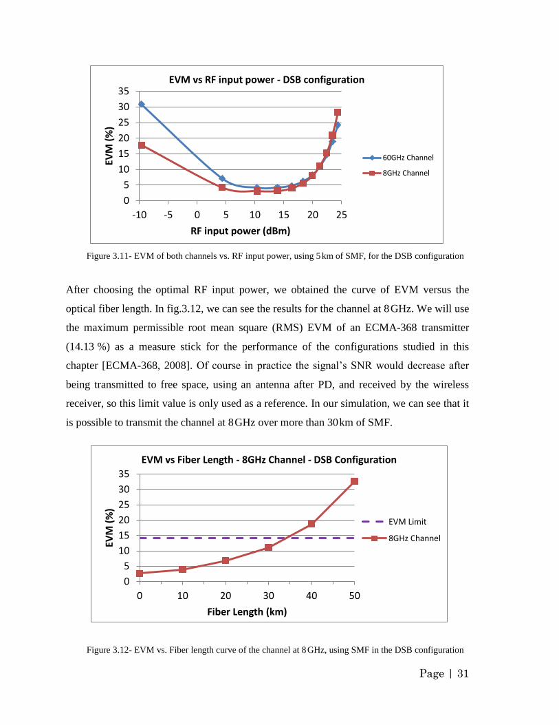
Figure 3.11- EVM of both channels vs. RF input power, using 5 km of SMF, for the DSB configuration
After choosing the optimal RF input power, we obtained the curve of EVM versus the
optical fiber length. In fig.3.12, we can see the results for the channel at 8 GHz. We will use
the maximum permissible root mean square (RMS) EVM of an ECMA-368 transmitter
(14.13 %) as a measure stick for the performance of the configurations studied in this
chapter [ECMA-368, 2008]. Of course in practice the signal‟s SNR would decrease after
being transmitted to free space, using an antenna after PD, and received by the wireless
receiver, so this limit value is only used as a reference. In our simulation, we can see that it
is possible to transmit the channel at 8 GHz over more than 30 km of SMF.
Figure 3.12- EVM vs. Fiber length curve of the channel at 8 GHz, using SMF in the DSB configuration
0
5
10
15
20
25
30
35
-10 -5 0 5 10 15 20 25
EVM
(%
)
RF input power (dBm)
EVM vs RF input power - DSB configuration
60GHz Channel
8GHz Channel
0
5
10
15
20
25
30
35
0 10 20 30 40 50
EVM
(%
)
Fiber Length (km)
EVM vs Fiber Length - 8GHz Channel - DSB Configuration
EVM Limit
8GHz Channel
Page | 32
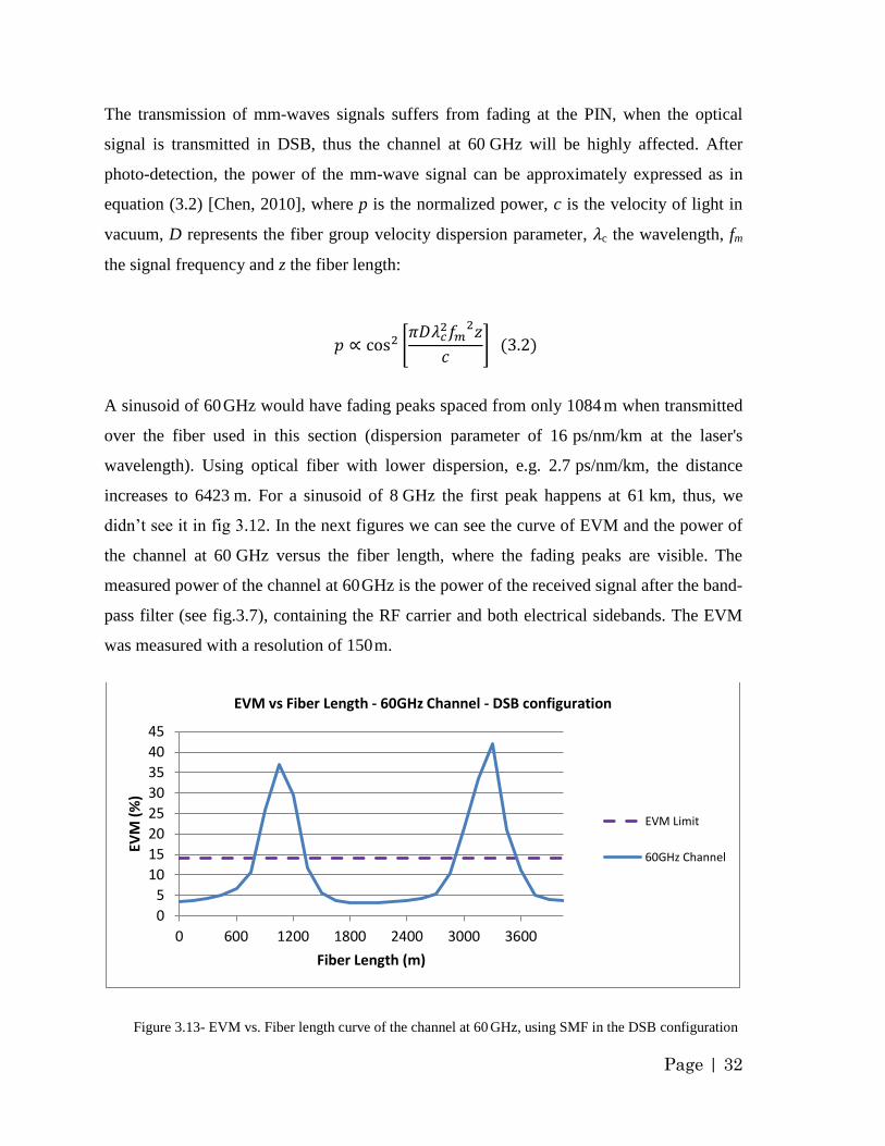
The transmission of mm-waves signals suffers from fading at the PIN, when the optical
signal is transmitted in DSB, thus the channel at 60 GHz will be highly affected. After
photo-detection, the power of the mm-wave signal can be approximately expressed as in
equation (3.2) [Chen, 2010], where p is the normalized power, c is the velocity of light in
vacuum, D represents the fiber group velocity dispersion parameter, 𝜆c the wavelength, fm
the signal frequency and z the fiber length:
[ 𝜆
] ( )
A sinusoid of 60 GHz would have fading peaks spaced from only 1084 m when transmitted
over the fiber used in this section (dispersion parameter of 16 ps/nm/km at the laser's
wavelength). Using optical fiber with lower dispersion, e.g. 2.7 ps/nm/km, the distance
increases to 6423 m. For a sinusoid of 8 GHz the first peak happens at 61 km, thus, we
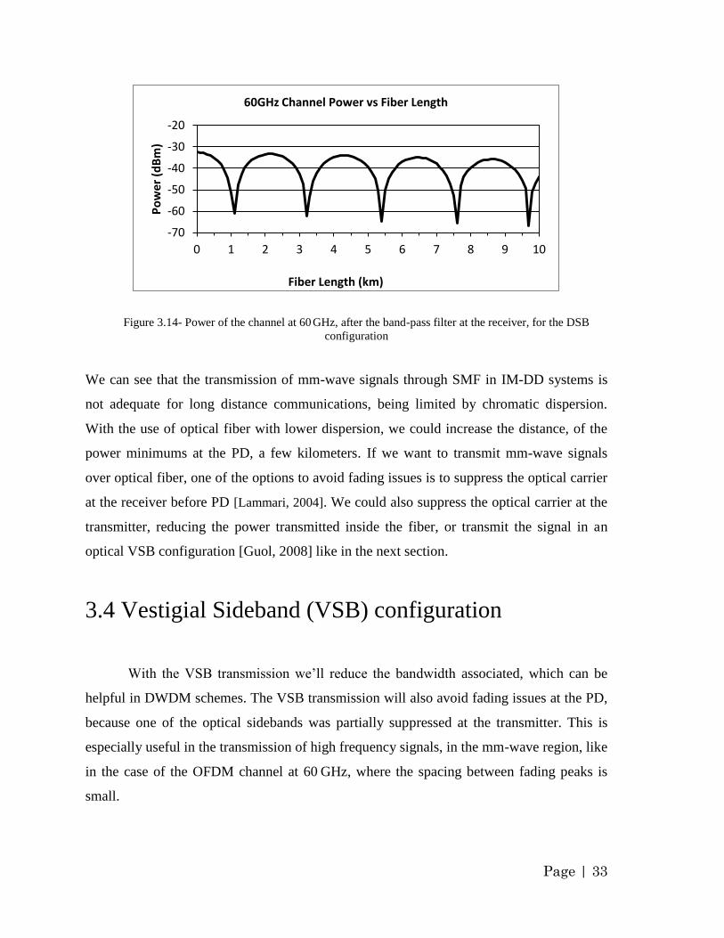
didn‟t see it in fig 3.12. In the next figures we can see the curve of EVM and the power of
the channel at 60 GHz versus the fiber length, where the fading peaks are visible. The
measured power of the channel at 60 GHz is the power of the received signal after the band-
pass filter (see fig.3.7), containing the RF carrier and both electrical sidebands. The EVM
was measured with a resolution of 150 m.
Figure 3.13- EVM vs. Fiber length curve of the channel at 60 GHz, using SMF in the DSB configuration
0
5
10
15
20
25
30
35
40
45
0 600 1200 1800 2400 3000 3600
EVM
(%
)
Fiber Length (m)
EVM vs Fiber Length - 60GHz Channel - DSB configuration
EVM Limit
60GHz Channel
Page | 33
Figure 3.14- Power of the channel at 60 GHz, after the band-pass filter at the receiver, for the DSB
configuration
We can see that the transmission of mm-wave signals through SMF in IM-DD systems is
not adequate for long distance communications, being limited by chromatic dispersion.
With the use of optical fiber with lower dispersion, we could increase the distance, of the
power minimums at the PD, a few kilometers. If we want to transmit mm-wave signals
over optical fiber, one of the options to avoid fading issues is to suppress the optical carrier
at the receiver before PD [Lammari, 2004]. We could also suppress the optical carrier at the
transmitter, reducing the power transmitted inside the fiber, or transmit the signal in an
optical VSB configuration [Guol, 2008] like in the next section.
3.4 Vestigial Sideband (VSB) configuration
With the VSB transmission we‟ll reduce the bandwidth associated, which can be
helpful in DWDM schemes. The VSB transmission will also avoid fading issues at the PD,
because one of the optical sidebands was partially suppressed at the transmitter. This is
especially useful in the transmission of high frequency signals, in the mm-wave region, like
in the case of the OFDM channel at 60 GHz, where the spacing between fading peaks is
small.
-70
-60
-50
-40
-30
-20
0 1 2 3 4 5 6 7 8 9 10
Po
wer
(d
Bm
)
Fiber Length (km)
60GHz Channel Power vs Fiber Length
Page | 34
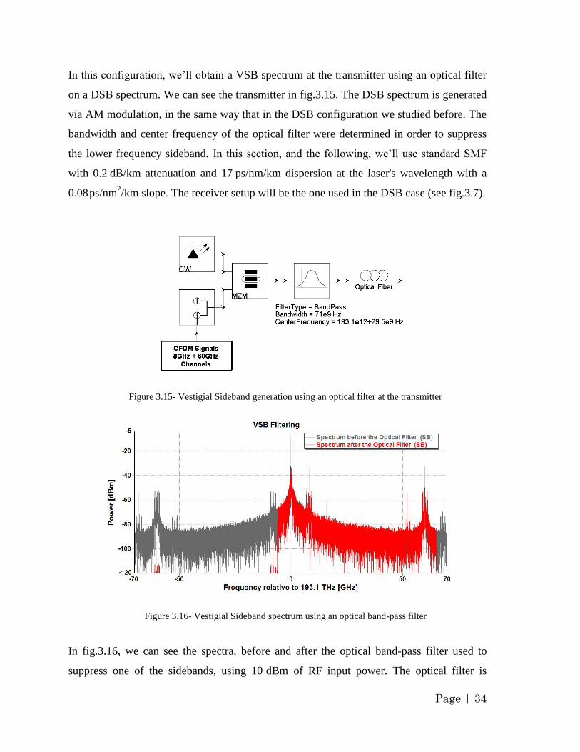
In this configuration, we‟ll obtain a VSB spectrum at the transmitter using an optical filter
on a DSB spectrum. We can see the transmitter in fig.3.15. The DSB spectrum is generated
via AM modulation, in the same way that in the DSB configuration we studied before. The
bandwidth and center frequency of the optical filter were determined in order to suppress
the lower frequency sideband. In this section, and the following, we‟ll use standard SMF
with 0.2 dB/km attenuation and 17 ps/nm/km dispersion at the laser's wavelength with a
0.08 ps/nm2/km slope. The receiver setup will be the one used in the DSB case (see fig.3.7).
Figure 3.15- Vestigial Sideband generation using an optical filter at the transmitter
Figure 3.16- Vestigial Sideband spectrum using an optical band-pass filter
In fig.3.16, we can see the spectra, before and after the optical band-pass filter used to
suppress one of the sidebands, using 10 dBm of RF input power. The optical filter is
Page | 35
considered almost ideal with 60 dB attenuation at the stop band, no attenuation at the pass
band, center frequency of 29.5 GHz relative to the laser's emission frequency and 71 GHz
bandwidth with a fast transition between the stop band and the pass band. We determined,
once again, the optimal RF input power by simulation, varying this value for a 10 km fiber
length and observing the EVM at the receiver after PD, resulting in 16 dBm.
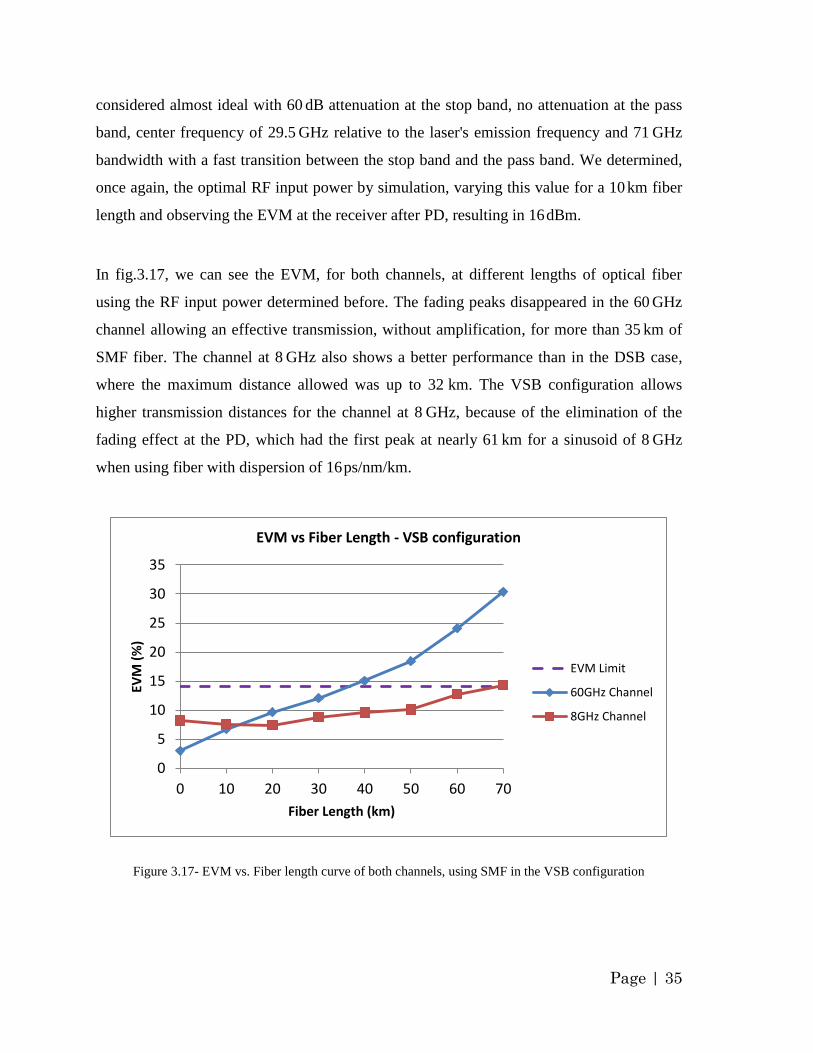
In fig.3.17, we can see the EVM, for both channels, at different lengths of optical fiber
using the RF input power determined before. The fading peaks disappeared in the 60 GHz
channel allowing an effective transmission, without amplification, for more than 35 km of
SMF fiber. The channel at 8 GHz also shows a better performance than in the DSB case,
where the maximum distance allowed was up to 32 km. The VSB configuration allows
higher transmission distances for the channel at 8 GHz, because of the elimination of the
fading effect at the PD, which had the first peak at nearly 61 km for a sinusoid of 8 GHz
when using fiber with dispersion of 16 ps/nm/km.
Figure 3.17- EVM vs. Fiber length curve of both channels, using SMF in the VSB configuration
0
5
10
15
20
25
30
35
0 10 20 30 40 50 60 70
EVM
(%
)
Fiber Length (km)
EVM vs Fiber Length - VSB configuration
EVM Limit
60GHz Channel
8GHz Channel
Page | 36
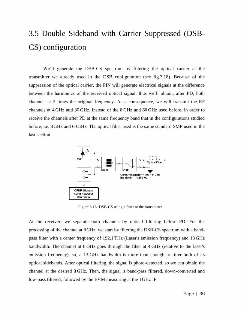
3.5 Double Sideband with Carrier Suppressed (DSB-
CS) configuration
We‟ll generate the DSB-CS spectrum by filtering the optical carrier at the
transmitter we already used in the DSB configuration (see fig.3.18). Because of the
suppression of the optical carrier, the PIN will generate electrical signals at the difference
between the harmonics of the received optical signal, thus we‟ll obtain, after PD, both
channels at 2 times the original frequency. As a consequence, we will transmit the RF
channels at 4 GHz and 30 GHz, instead of the 8 GHz and 60 GHz used before, in order to
receive the channels after PD at the same frequency band that in the configurations studied
before, i.e. 8 GHz and 60 GHz. The optical fiber used is the same standard SMF used in the
last section.
Figure 3.18- DSB-CS using a filter at the transmitter
At the receiver, we separate both channels by optical filtering before PD. For the
processing of the channel at 8 GHz, we start by filtering the DSB-CS spectrum with a band-
pass filter with a center frequency of 192.1 THz (Laser's emission frequency) and 13 GHz
bandwidth. The channel at 8 GHz goes through the fiber at 4 GHz (relative to the laser's
emission frequency), so, a 13 GHz bandwidth is more than enough to filter both of its
optical sidebands. After optical filtering, the signal is photo-detected, so we can obtain the
channel at the desired 8 GHz. Then, the signal is band-pass filtered, down-converted and
low-pass filtered, followed by the EVM measuring at the 1 GHz IF.
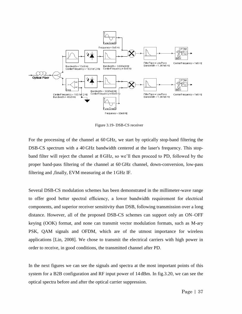
Page | 37
Figure 3.19- DSB-CS receiver
For the processing of the channel at 60 GHz, we start by optically stop-band filtering the
DSB-CS spectrum with a 40 GHz bandwidth centered at the laser's frequency. This stop-
band filter will reject the channel at 8 GHz, so we‟ll then proceed to PD, followed by the
proper band-pass filtering of the channel at 60 GHz channel, down-conversion, low-pass
filtering and ,finally, EVM measuring at the 1 GHz IF.
Several DSB-CS modulation schemes has been demonstrated in the millimeter-wave range
to offer good better spectral efficiency, a lower bandwidth requirement for electrical
components, and superior receiver sensitivity than DSB, following transmission over a long
distance. However, all of the proposed DSB-CS schemes can support only an ON–OFF
keying (OOK) format, and none can transmit vector modulation formats, such as M-ary
PSK, QAM signals and OFDM, which are of the utmost importance for wireless
applications [Lin, 2008]. We chose to transmit the electrical carriers with high power in
order to receive, in good conditions, the transmitted channel after PD.
In the next figures we can see the signals and spectra at the most important points of this
system for a B2B configuration and RF input power of 14 dBm. In fig.3.20, we can see the
optical spectra before and after the optical carrier suppression.
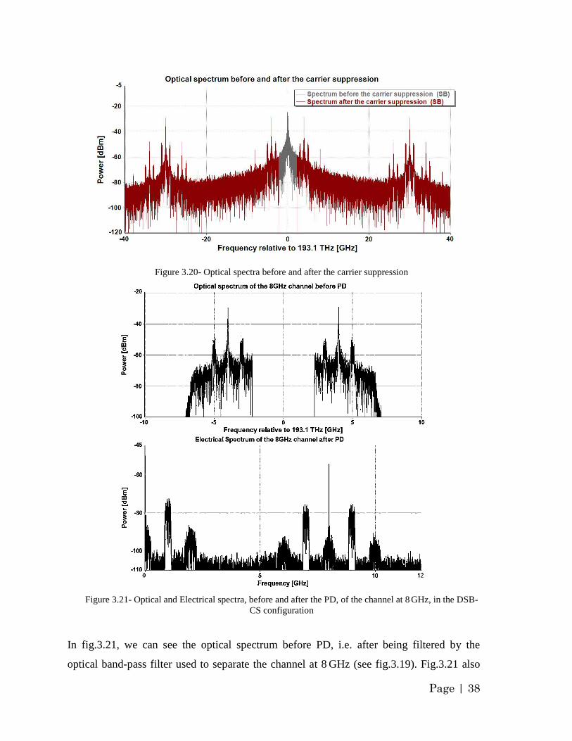
Page | 38
Figure 3.20- Optical spectra before and after the carrier suppression
Figure 3.21- Optical and Electrical spectra, before and after the PD, of the channel at 8 GHz, in the DSB-
CS configuration
In fig.3.21, we can see the optical spectrum before PD, i.e. after being filtered by the
optical band-pass filter used to separate the channel at 8 GHz (see fig.3.19). Fig.3.21 also
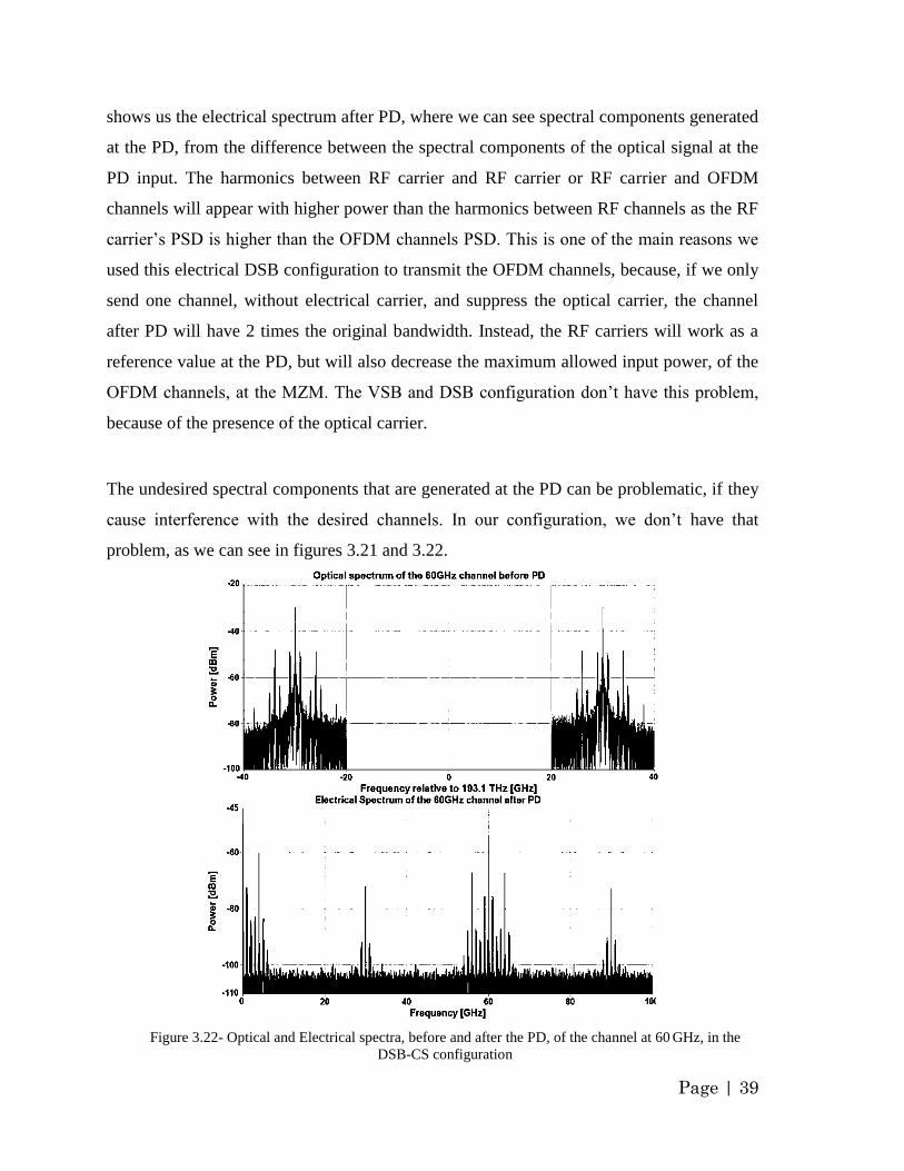
Page | 39
shows us the electrical spectrum after PD, where we can see spectral components generated
at the PD, from the difference between the spectral components of the optical signal at the
PD input. The harmonics between RF carrier and RF carrier or RF carrier and OFDM
channels will appear with higher power than the harmonics between RF channels as the RF
carrier‟s PSD is higher than the OFDM channels PSD. This is one of the main reasons we
used this electrical DSB configuration to transmit the OFDM channels, because, if we only
send one channel, without electrical carrier, and suppress the optical carrier, the channel
after PD will have 2 times the original bandwidth. Instead, the RF carriers will work as a
reference value at the PD, but will also decrease the maximum allowed input power, of the
OFDM channels, at the MZM. The VSB and DSB configuration don‟t have this problem,
because of the presence of the optical carrier.
The undesired spectral components that are generated at the PD can be problematic, if they
cause interference with the desired channels. In our configuration, we don‟t have that
problem, as we can see in figures 3.21 and 3.22.
Figure 3.22- Optical and Electrical spectra, before and after the PD, of the channel at 60 GHz, in the
DSB-CS configuration
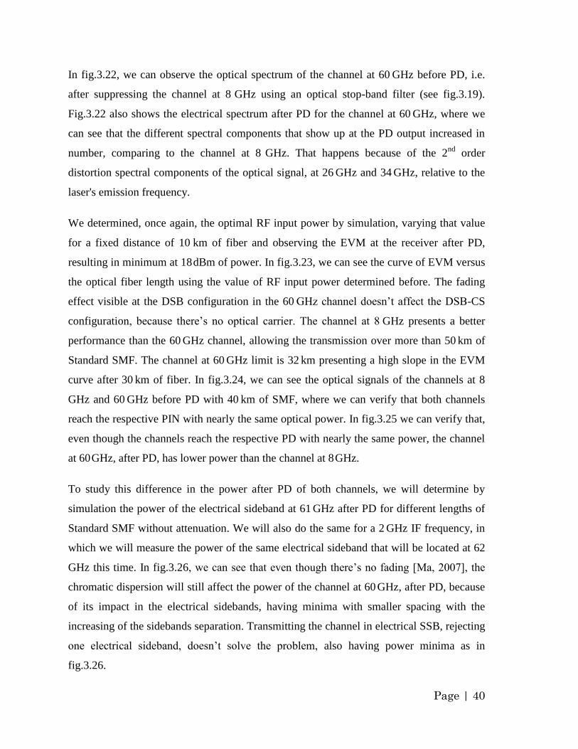
Page | 40
In fig.3.22, we can observe the optical spectrum of the channel at 60 GHz before PD, i.e.
after suppressing the channel at 8 GHz using an optical stop-band filter (see fig.3.19).
Fig.3.22 also shows the electrical spectrum after PD for the channel at 60 GHz, where we
can see that the different spectral components that show up at the PD output increased in
number, comparing to the channel at 8 GHz. That happens because of the 2nd
order
distortion spectral components of the optical signal, at 26 GHz and 34 GHz, relative to the
laser's emission frequency.
We determined, once again, the optimal RF input power by simulation, varying that value
for a fixed distance of 10 km of fiber and observing the EVM at the receiver after PD,
resulting in minimum at 18 dBm of power. In fig.3.23, we can see the curve of EVM versus
the optical fiber length using the value of RF input power determined before. The fading
effect visible at the DSB configuration in the 60 GHz channel doesn‟t affect the DSB-CS
configuration, because there‟s no optical carrier. The channel at 8 GHz presents a better
performance than the 60 GHz channel, allowing the transmission over more than 50 km of
Standard SMF. The channel at 60 GHz limit is 32 km presenting a high slope in the EVM
curve after 30 km of fiber. In fig.3.24, we can see the optical signals of the channels at 8
GHz and 60 GHz before PD with 40 km of SMF, where we can verify that both channels
reach the respective PIN with nearly the same optical power. In fig.3.25 we can verify that,
even though the channels reach the respective PD with nearly the same power, the channel
at 60 GHz, after PD, has lower power than the channel at 8 GHz.
To study this difference in the power after PD of both channels, we will determine by
simulation the power of the electrical sideband at 61 GHz after PD for different lengths of
Standard SMF without attenuation. We will also do the same for a 2 GHz IF frequency, in
which we will measure the power of the same electrical sideband that will be located at 62
GHz this time. In fig.3.26, we can see that even though there‟s no fading [Ma, 2007], the
chromatic dispersion will still affect the power of the channel at 60 GHz, after PD, because
of its impact in the electrical sidebands, having minima with smaller spacing with the
increasing of the sidebands separation. Transmitting the channel in electrical SSB, rejecting
one electrical sideband, doesn‟t solve the problem, also having power minima as in
fig.3.26.
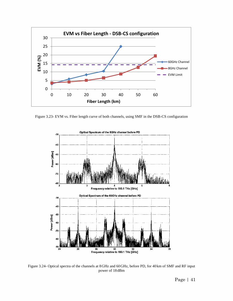
Page | 41
Figure 3.23- EVM vs. Fiber length curve of both channels, using SMF in the DSB-CS configuration
Figure 3.24- Optical spectra of the channels at 8 GHz and 60 GHz, before PD, for 40 km of SMF and RF input
power of 18 dBm
0
5
10
15
20
25
30
0 10 20 30 40 50 60
EVM
(%
)
Fiber Length (km)
EVM vs Fiber Length - DSB-CS configuration
60GHz Channel
8GHz Channel
EVM Limit
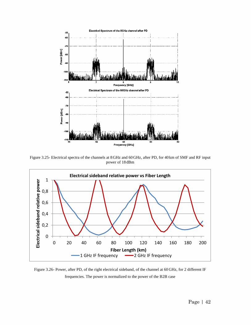
Page | 42
Figure 3.25- Electrical spectra of the channels at 8 GHz and 60 GHz, after PD, for 40 km of SMF and RF input
power of 18 dBm
Figure 3.26- Power, after PD, of the right electrical sideband, of the channel at 60 GHz, for 2 different IF
frequencies. The power is normalized to the power of the B2B case
0
0,2
0,4
0,6
0,8
1
0 20 40 60 80 100 120 140 160 180 200
Elec
tric
al s
ideb
and
rel
ativ
e p
ow
er
Fiber Length (km)
Electrical sideband relative power vs Fiber Length
1 GHz IF frequency 2 GHz IF frequency
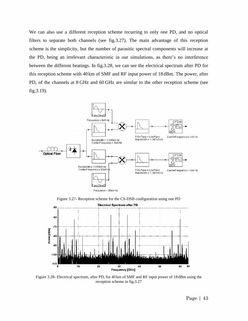
Page | 43
We can also use a different reception scheme recurring to only one PD, and no optical
filters to separate both channels (see fig.3.27). The main advantage of this reception
scheme is the simplicity, but the number of parasitic spectral components will increase at
the PD, being an irrelevant characteristic in our simulations, as there‟s no interference
between the different beatings. In fig.3.28, we can see the electrical spectrum after PD for
this reception scheme with 40 km of SMF and RF input power of 18 dBm. The power, after
PD, of the channels at 8 GHz and 60 GHz are similar to the other reception scheme (see
fig.3.19).
Figure 3.27- Reception scheme for the CS-DSB configuration using one PD
Figure 3.28- Electrical spectrum, after PD, for 40 km of SMF and RF input power of 18 dBm using the
reception scheme in fig.3.27
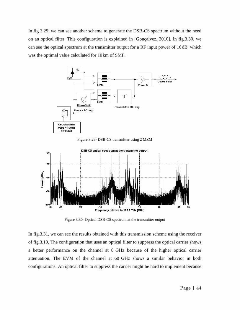
Page | 44
In fig 3.29, we can see another scheme to generate the DSB-CS spectrum without the need
on an optical filter. This configuration is explained in [Gonçalvez, 2010]. In fig.3.30, we
can see the optical spectrum at the transmitter output for a RF input power of 16 dB, which
was the optimal value calculated for 10 km of SMF.
Figure 3.29- DSB-CS transmitter using 2 MZM
Figure 3.30- Optical DSB-CS spectrum at the transmitter output
In fig.3.31, we can see the results obtained with this transmission scheme using the receiver
of fig.3.19. The configuration that uses an optical filter to suppress the optical carrier shows
a better performance on the channel at 8 GHz because of the higher optical carrier
attenuation. The EVM of the channel at 60 GHz shows a similar behavior in both
configurations. An optical filter to suppress the carrier might be hard to implement because
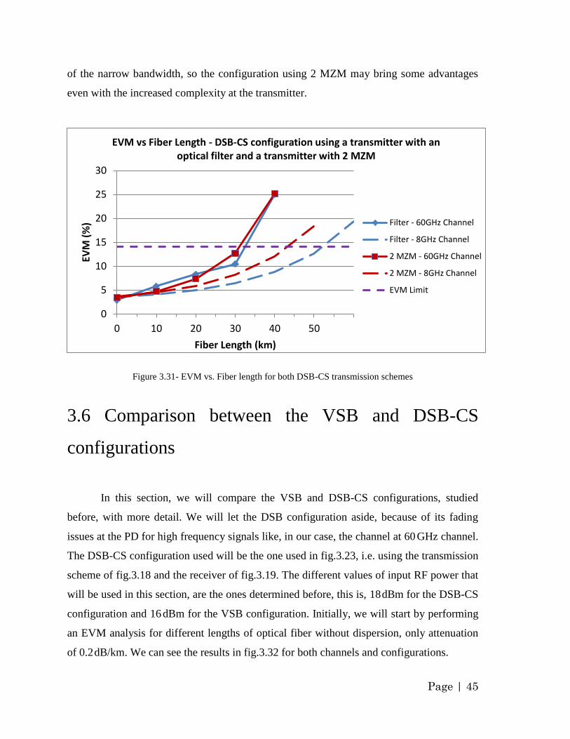
Page | 45
of the narrow bandwidth, so the configuration using 2 MZM may bring some advantages
even with the increased complexity at the transmitter.
Figure 3.31- EVM vs. Fiber length for both DSB-CS transmission schemes
3.6 Comparison between the VSB and DSB-CS
configurations
In this section, we will compare the VSB and DSB-CS configurations, studied
before, with more detail. We will let the DSB configuration aside, because of its fading
issues at the PD for high frequency signals like, in our case, the channel at 60 GHz channel.
The DSB-CS configuration used will be the one used in fig.3.23, i.e. using the transmission
scheme of fig.3.18 and the receiver of fig.3.19. The different values of input RF power that
will be used in this section, are the ones determined before, this is, 18 dBm for the DSB-CS
configuration and 16 dBm for the VSB configuration. Initially, we will start by performing
an EVM analysis for different lengths of optical fiber without dispersion, only attenuation
of 0.2 dB/km. We can see the results in fig.3.32 for both channels and configurations.
0
5
10
15
20
25
30
0 10 20 30 40 50
EVM
(%
)
Fiber Length (km)
EVM vs Fiber Length - DSB-CS configuration using a transmitter with an optical filter and a transmitter with 2 MZM
Filter - 60GHz Channel
Filter - 8GHz Channel
2 MZM - 60GHz Channel
2 MZM - 8GHz Channel
EVM Limit
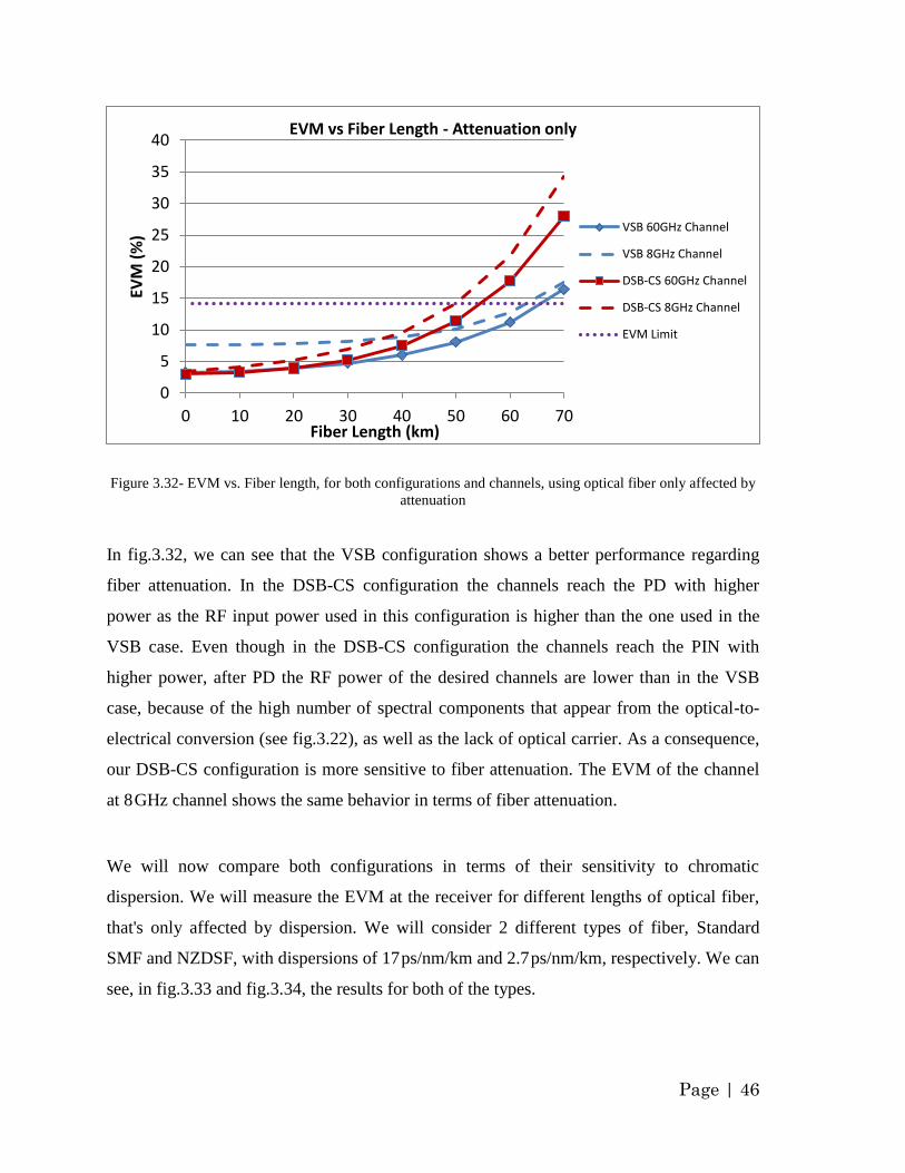
Page | 46
Figure 3.32- EVM vs. Fiber length, for both configurations and channels, using optical fiber only affected by
attenuation
In fig.3.32, we can see that the VSB configuration shows a better performance regarding
fiber attenuation. In the DSB-CS configuration the channels reach the PD with higher
power as the RF input power used in this configuration is higher than the one used in the
VSB case. Even though in the DSB-CS configuration the channels reach the PIN with
higher power, after PD the RF power of the desired channels are lower than in the VSB
case, because of the high number of spectral components that appear from the optical-to-
electrical conversion (see fig.3.22), as well as the lack of optical carrier. As a consequence,
our DSB-CS configuration is more sensitive to fiber attenuation. The EVM of the channel
at 8 GHz channel shows the same behavior in terms of fiber attenuation.
We will now compare both configurations in terms of their sensitivity to chromatic
dispersion. We will measure the EVM at the receiver for different lengths of optical fiber,
that's only affected by dispersion. We will consider 2 different types of fiber, Standard
SMF and NZDSF, with dispersions of 17 ps/nm/km and 2.7 ps/nm/km, respectively. We can
see, in fig.3.33 and fig.3.34, the results for both of the types.
0
5
10
15
20
25
30
35
40
0 10 20 30 40 50 60 70
EVM
(%
)
Fiber Length (km)
EVM vs Fiber Length - Attenuation only
VSB 60GHz Channel
VSB 8GHz Channel
DSB-CS 60GHz Channel
DSB-CS 8GHz Channel
EVM Limit
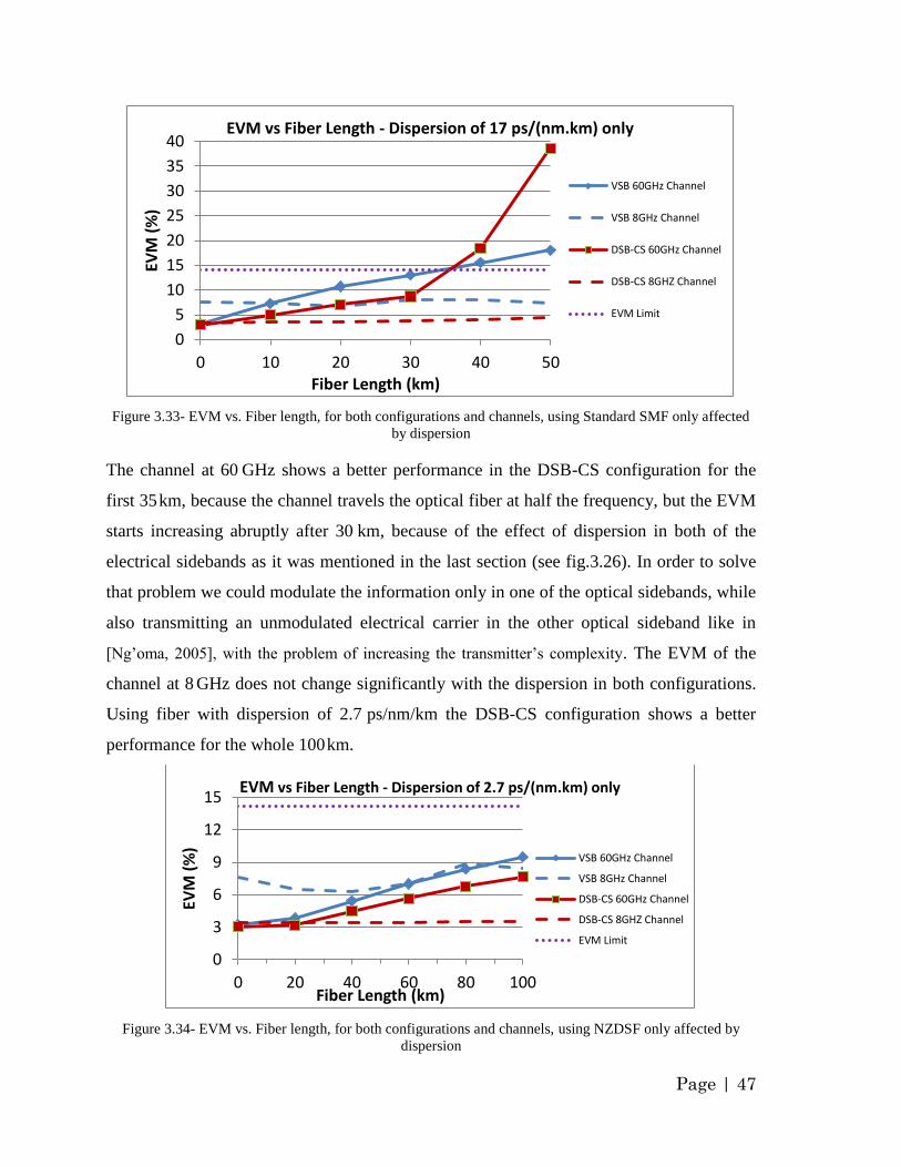
Page | 47
Figure 3.33- EVM vs. Fiber length, for both configurations and channels, using Standard SMF only affected
by dispersion
The channel at 60 GHz shows a better performance in the DSB-CS configuration for the
first 35 km, because the channel travels the optical fiber at half the frequency, but the EVM
starts increasing abruptly after 30 km, because of the effect of dispersion in both of the
electrical sidebands as it was mentioned in the last section (see fig.3.26). In order to solve
that problem we could modulate the information only in one of the optical sidebands, while
also transmitting an unmodulated electrical carrier in the other optical sideband like in
[Ng‟oma, 2005], with the problem of increasing the transmitter‟s complexity. The EVM of the
channel at 8 GHz does not change significantly with the dispersion in both configurations.
Using fiber with dispersion of 2.7 ps/nm/km the DSB-CS configuration shows a better
performance for the whole 100 km.
Figure 3.34- EVM vs. Fiber length, for both configurations and channels, using NZDSF only affected by
dispersion
0
5
10
15
20
25
30
35
40
0 10 20 30 40 50
EVM
(%
)
Fiber Length (km)
EVM vs Fiber Length - Dispersion of 17 ps/(nm.km) only
VSB 60GHz Channel
VSB 8GHz Channel
DSB-CS 60GHz Channel
DSB-CS 8GHZ Channel
EVM Limit
0
3
6
9
12
15
0 20 40 60 80 100
EVM
(%
)
Fiber Length (km)
EVM vs Fiber Length - Dispersion of 2.7 ps/(nm.km) only
VSB 60GHz Channel
VSB 8GHz Channel
DSB-CS 60GHz Channel
DSB-CS 8GHZ Channel
EVM Limit
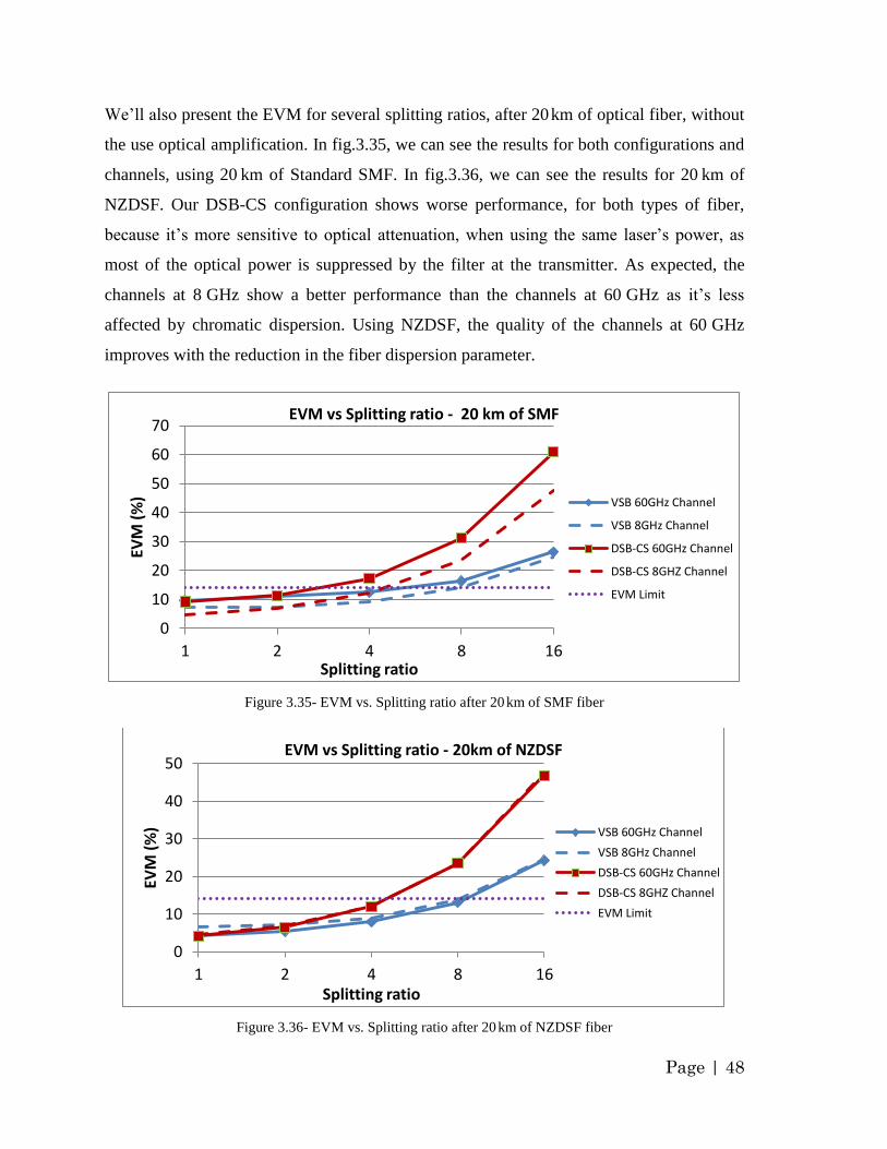
Page | 48
We‟ll also present the EVM for several splitting ratios, after 20 km of optical fiber, without
the use optical amplification. In fig.3.35, we can see the results for both configurations and
channels, using 20 km of Standard SMF. In fig.3.36, we can see the results for 20 km of
NZDSF. Our DSB-CS configuration shows worse performance, for both types of fiber,
because it‟s more sensitive to optical attenuation, when using the same laser‟s power, as
most of the optical power is suppressed by the filter at the transmitter. As expected, the
channels at 8 GHz show a better performance than the channels at 60 GHz as it‟s less
affected by chromatic dispersion. Using NZDSF, the quality of the channels at 60 GHz
improves with the reduction in the fiber dispersion parameter.
Figure 3.35- EVM vs. Splitting ratio after 20 km of SMF fiber
Figure 3.36- EVM vs. Splitting ratio after 20 km of NZDSF fiber
0
10
20
30
40
50
60
70
1 2 4 8 16
EVM
(%
)
Splitting ratio
EVM vs Splitting ratio - 20 km of SMF
VSB 60GHz Channel
VSB 8GHz Channel
DSB-CS 60GHz Channel
DSB-CS 8GHZ Channel
EVM Limit
0
10
20
30
40
50
1 2 4 8 16
EVM
(%
)
Splitting ratio
EVM vs Splitting ratio - 20km of NZDSF
VSB 60GHz Channel
VSB 8GHz Channel
DSB-CS 60GHz Channel
DSB-CS 8GHZ Channel
EVM Limit
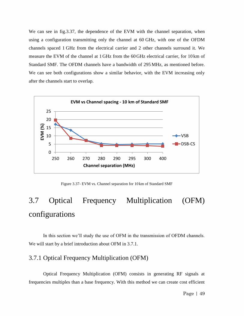
Page | 49
We can see in fig.3.37, the dependence of the EVM with the channel separation, when
using a configuration transmitting only the channel at 60 GHz, with one of the OFDM
channels spaced 1 GHz from the electrical carrier and 2 other channels surround it. We
measure the EVM of the channel at 1 GHz from the 60 GHz electrical carrier, for 10 km of
Standard SMF. The OFDM channels have a bandwidth of 295 MHz, as mentioned before.
We can see both configurations show a similar behavior, with the EVM increasing only
after the channels start to overlap.
Figure 3.37- EVM vs. Channel separation for 10 km of Standard SMF
3.7 Optical Frequency Multiplication (OFM)
configurations
In this section we‟ll study the use of OFM in the transmission of OFDM channels.
We will start by a brief introduction about OFM in 3.7.1.
3.7.1 Optical Frequency Multiplication (OFM)
Optical Frequency Multiplication (OFM) consists in generating RF signals at
frequencies multiples than a base frequency. With this method we can create cost efficient
0
5
10
15
20
25
250 260 270 280 290 295 300 400
EVM
(%
)
Channel separation (MHz)
EVM vs Channel spacing - 10 km of Standard SMF
VSB
DSB-CS
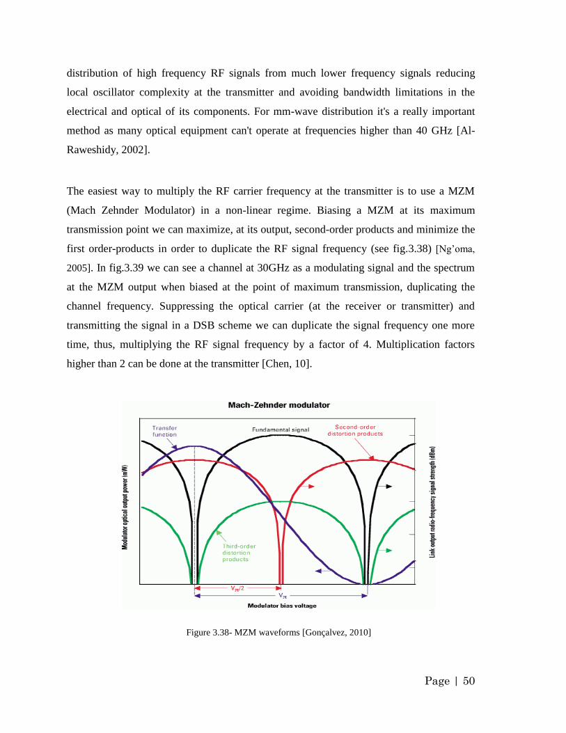
Page | 50
distribution of high frequency RF signals from much lower frequency signals reducing
local oscillator complexity at the transmitter and avoiding bandwidth limitations in the
electrical and optical of its components. For mm-wave distribution it's a really important
method as many optical equipment can't operate at frequencies higher than 40 GHz [Al-
Raweshidy, 2002].
The easiest way to multiply the RF carrier frequency at the transmitter is to use a MZM
(Mach Zehnder Modulator) in a non-linear regime. Biasing a MZM at its maximum
transmission point we can maximize, at its output, second-order products and minimize the
first order-products in order to duplicate the RF signal frequency (see fig.3.38) [Ng‟oma,
2005]. In fig.3.39 we can see a channel at 30GHz as a modulating signal and the spectrum
at the MZM output when biased at the point of maximum transmission, duplicating the
channel frequency. Suppressing the optical carrier (at the receiver or transmitter) and
transmitting the signal in a DSB scheme we can duplicate the signal frequency one more
time, thus, multiplying the RF signal frequency by a factor of 4. Multiplication factors
higher than 2 can be done at the transmitter [Chen, 10].
Figure 3.38- MZM waveforms [Gonçalvez, 2010]
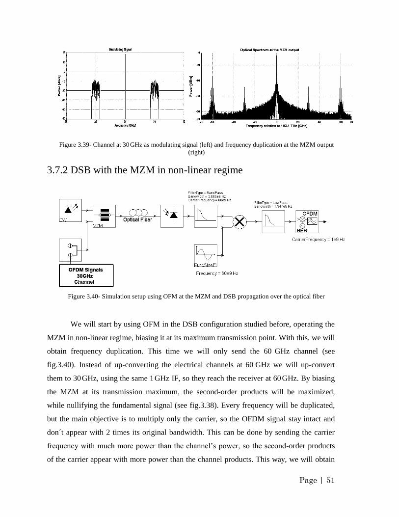
Page | 51
Figure 3.39- Channel at 30 GHz as modulating signal (left) and frequency duplication at the MZM output
(right)
3.7.2 DSB with the MZM in non-linear regime
Figure 3.40- Simulation setup using OFM at the MZM and DSB propagation over the optical fiber
We will start by using OFM in the DSB configuration studied before, operating the
MZM in non-linear regime, biasing it at its maximum transmission point. With this, we will
obtain frequency duplication. This time we will only send the 60 GHz channel (see
fig.3.40). Instead of up-converting the electrical channels at 60 GHz we will up-convert
them to 30 GHz, using the same 1 GHz IF, so they reach the receiver at 60 GHz. By biasing
the MZM at its transmission maximum, the second-order products will be maximized,
while nullifying the fundamental signal (see fig.3.38). Every frequency will be duplicated,
but the main objective is to multiply only the carrier, so the OFDM signal stay intact and
don´t appear with 2 times its original bandwidth. This can be done by sending the carrier
frequency with much more power than the channel‟s power, so the second-order products
of the carrier appear with more power than the channel products. This way, we will obtain
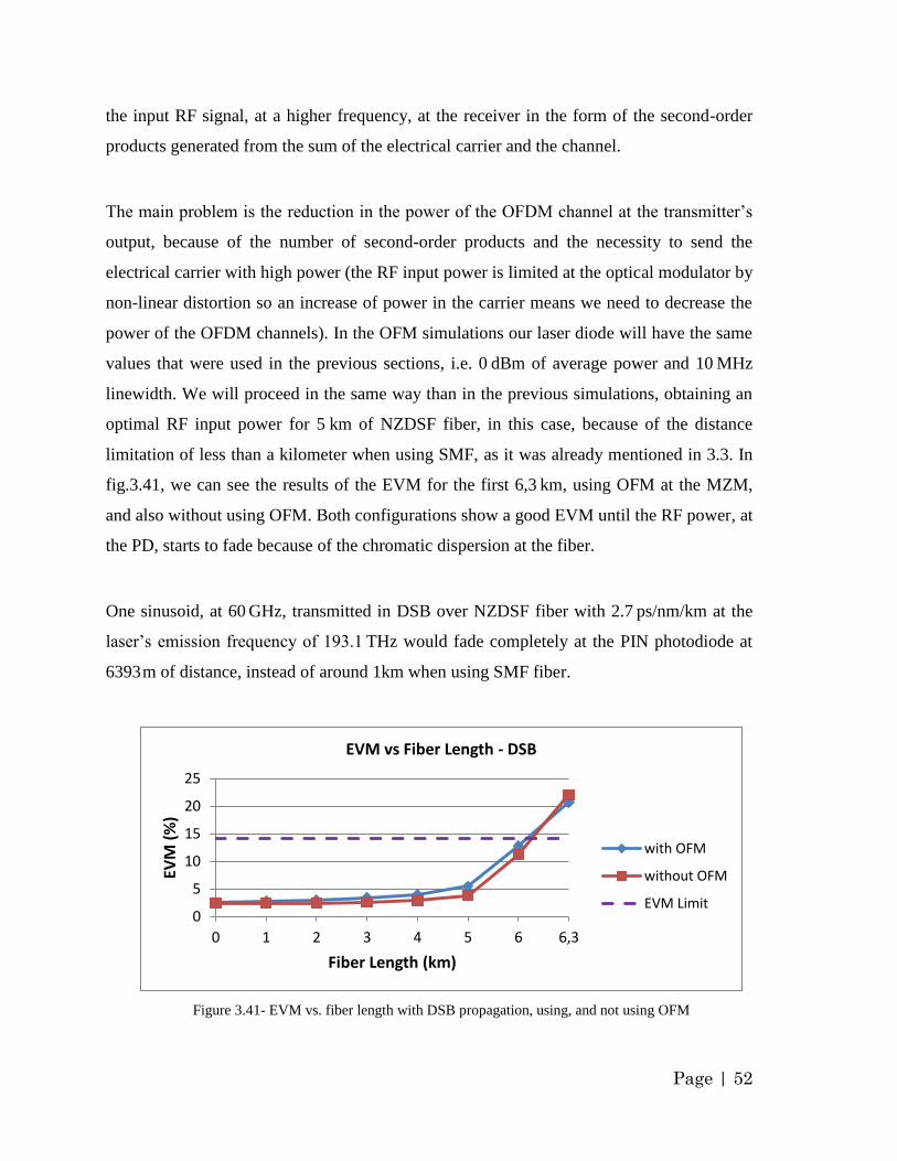
Page | 52
the input RF signal, at a higher frequency, at the receiver in the form of the second-order
products generated from the sum of the electrical carrier and the channel.
The main problem is the reduction in the power of the OFDM channel at the transmitter‟s
output, because of the number of second-order products and the necessity to send the
electrical carrier with high power (the RF input power is limited at the optical modulator by
non-linear distortion so an increase of power in the carrier means we need to decrease the
power of the OFDM channels). In the OFM simulations our laser diode will have the same
values that were used in the previous sections, i.e. 0 dBm of average power and 10 MHz
linewidth. We will proceed in the same way than in the previous simulations, obtaining an
optimal RF input power for 5 km of NZDSF fiber, in this case, because of the distance
limitation of less than a kilometer when using SMF, as it was already mentioned in 3.3. In
fig.3.41, we can see the results of the EVM for the first 6,3 km, using OFM at the MZM,
and also without using OFM. Both configurations show a good EVM until the RF power, at
the PD, starts to fade because of the chromatic dispersion at the fiber.
One sinusoid, at 60 GHz, transmitted in DSB over NZDSF fiber with 2.7 ps/nm/km at the
laser‟s emission frequency of 193.1 THz would fade completely at the PIN photodiode at
6393 m of distance, instead of around 1km when using SMF fiber.
Figure 3.41- EVM vs. fiber length with DSB propagation, using, and not using OFM
0
5
10
15
20
25
0 1 2 3 4 5 6 6,3
EVM
(%
)
Fiber Length (km)
EVM vs Fiber Length - DSB
with OFM
without OFM
EVM Limit
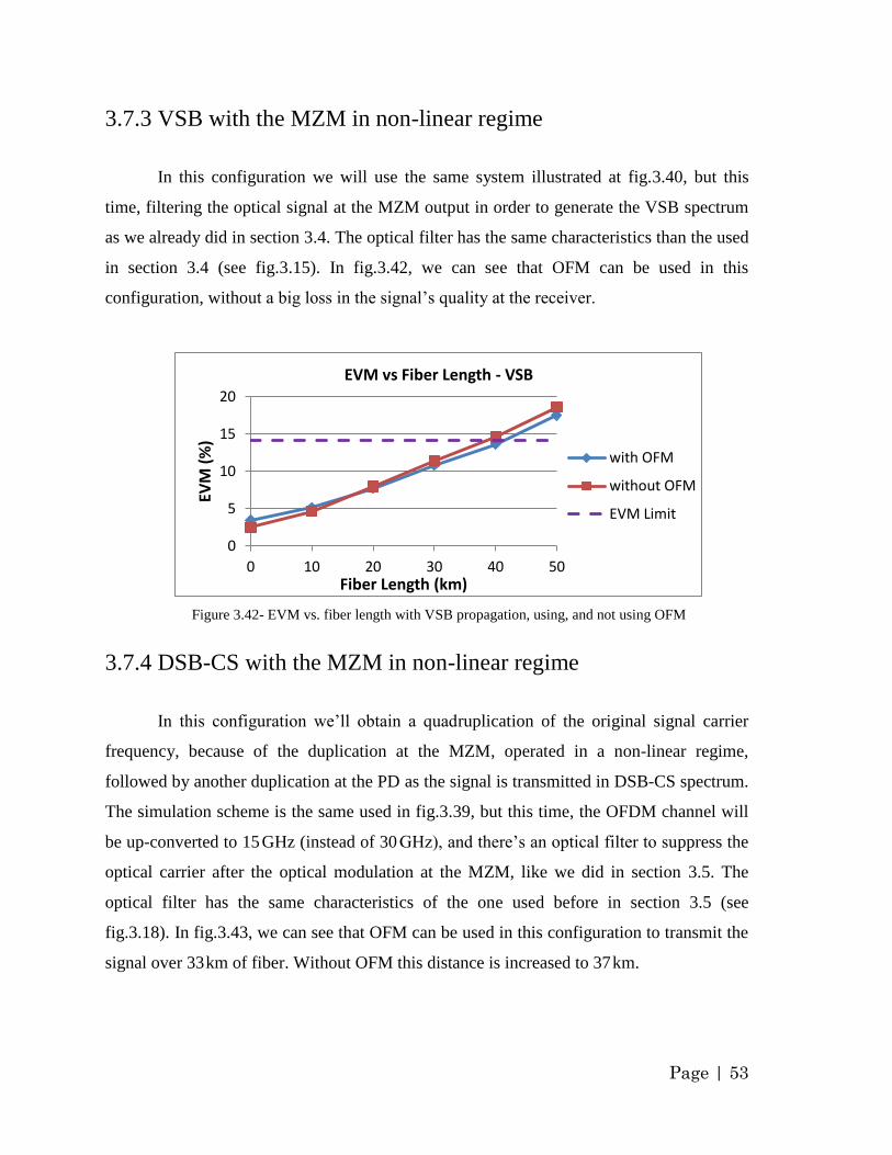
Page | 53
3.7.3 VSB with the MZM in non-linear regime
In this configuration we will use the same system illustrated at fig.3.40, but this
time, filtering the optical signal at the MZM output in order to generate the VSB spectrum
as we already did in section 3.4. The optical filter has the same characteristics than the used
in section 3.4 (see fig.3.15). In fig.3.42, we can see that OFM can be used in this
configuration, without a big loss in the signal‟s quality at the receiver.
Figure 3.42- EVM vs. fiber length with VSB propagation, using, and not using OFM
3.7.4 DSB-CS with the MZM in non-linear regime
In this configuration we‟ll obtain a quadruplication of the original signal carrier
frequency, because of the duplication at the MZM, operated in a non-linear regime,
followed by another duplication at the PD as the signal is transmitted in DSB-CS spectrum.
The simulation scheme is the same used in fig.3.39, but this time, the OFDM channel will
be up-converted to 15 GHz (instead of 30 GHz), and there‟s an optical filter to suppress the
optical carrier after the optical modulation at the MZM, like we did in section 3.5. The
optical filter has the same characteristics of the one used before in section 3.5 (see
fig.3.18). In fig.3.43, we can see that OFM can be used in this configuration to transmit the
signal over 33 km of fiber. Without OFM this distance is increased to 37 km.
0
5
10
15
20
0 10 20 30 40 50
EVM
(%
)
Fiber Length (km)
EVM vs Fiber Length - VSB
with OFM
without OFM
EVM Limit
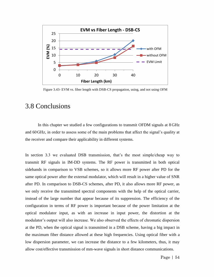
Page | 54
Figure 3.43- EVM vs. fiber length with DSB-CS propagation, using, and not using OFM
3.8 Conclusions
In this chapter we studied a few configurations to transmit OFDM signals at 8 GHz
and 60 GHz, in order to assess some of the main problems that affect the signal‟s quality at
the receiver and compare their applicability in different systems.
In section 3.3 we evaluated DSB transmission, that‟s the most simple/cheap way to
transmit RF signals in IM-DD systems. The RF power is transmitted in both optical
sidebands in comparison to VSB schemes, so it allows more RF power after PD for the
same optical power after the external modulator, which will result in a higher value of SNR
after PD. In comparison to DSB-CS schemes, after PD, it also allows more RF power, as
we only receive the transmitted spectral components with the help of the optical carrier,
instead of the large number that appear because of its suppression. The efficiency of the
configuration in terms of RF power is important because of the power limitation at the
optical modulator input, as with an increase in input power, the distortion at the
modulator‟s output will also increase. We also observed the effects of chromatic dispersion
at the PD, when the optical signal is transmitted in a DSB scheme, having a big impact in
the maximum fiber distance allowed at these high frequencies. Using optical fiber with a
low dispersion parameter, we can increase the distance to a few kilometers, thus, it may
allow cost/effective transmission of mm-wave signals in short distance communications.
0
5
10
15
20
25
0 10 20 30 40
EVM
(%
)
Fiber Length (km)
EVM vs Fiber Length - DSB-CS
with OFM
without OFM
EVM Limit
Page | 55
In section 3.4, we studied a configuration in VSB, recurring to an optical filter to suppress
one the optical sidebands. We could see that this in an effective way to eliminate the fading
effects that happened in the DSB configuration, bringing a big advantage for high
frequency signals, like in the mm-wave band. The main drawback is the increase in
complexity at the transmitter, because of the introduction of the optical filter.
In section 3.5, we studied the transmission in DSB-CS, recurring to several schemes. One
of the main advantages in this system is the duplication in frequency at the PD, so the
channel can be transmitted along the fiber at a lower frequency, being less affected by
chromatic dispersion, while also allowing local oscillators at lower frequencies at the
transmitter. Generating the electrical signals will reduce the bandwidth requirements of the
transmitter‟s components, something that can be really important in the transmission of
mm-wave radio signals. The main problem is that the duplication in frequency, at the PD,
would also duplicate the channel‟s bandwidth, something that has to be avoided as we do
not want to modify the generated OFDM channel. To avoid that problem, the channel
needs to have a reference value, as the optical carrier was suppressed. In order to do that,
we transmitted the electrical carrier over the fiber, with enough power, so the beatings of
the carrier with the OFDM channel generated at the PD can be measured at the OFDM
analyzer. The addition of the electrical carrier would reduce the possible power of the
OFDM channel at the modulator input. In the DSB and VSB we could easily transmit the
channels without any kind of reference value, allowing a higher input power on the OFDM
channels for the same optical carrier. Changing the power difference between the electrical
carriers and electrical sidebands, we couldn‟t improve the performance of the DSB-CS
system, as the values used in this chapter originated the better results.
Increasing the laser‟s power is a good way to improve the performance in this
configuration, as the power launched to the fiber is too low because of the carrier
suppression. In analog links is important to increase the power launched to the fiber as
possible, while not exceeding the SBS threshold that is the main limitative fiber non-linear
effect in these systems [Phillips, 1998].
Page | 56
In section 3.6 we could see that the DSB-CS configuration shows a better tolerance to fiber
dispersion because of the lower RF frequency, while the VSB configuration has a better
tolerance to attenuation, for the same laser power, while is a most straight-forward
configuration because of the presence of the optical carrier which will reduce second-order
distortion at the PD.
In section 3.7 we observed some of the advantages that OFM might bring when
transmitting mm-wave signals over fiber, allowing a multiplication factor of 2, at the
transmitter, when biasing the MZM at its maximum transmission point, thus, reducing
bandwidth restrictions at its components. The channel would also be multiplied in
bandwidth at the MZM‟s output, so the reference value is needed in a similar way than in
the DSB-CS schemes, having the same disadvantages mentioned previously. We could see
that the propagation of these signals over the optical fiber, after multiplication in the MZM,
doesn‟t show big degradation in the signal‟s quality.
Considering everything mentioned in this section, in IM-DD systems, DSB transmission
seems to be the preferable choice, wherever chromatic dispersion doesn‟t impose a strict
limit, in the maximum distance allowed, by fading issues at the PD, as it‟s the most simple
and cheap way to transmit the radio signals over fiber. With the use of lower dispersion
fiber, we can even transmit signals of frequencies around 60 GHz, for a few kms. When we
require long distance transmission of high frequency radio signals, VSB transmission
seems to be the more effective method to do it. The main advantage of the use of VSB
transmission, with Standard SMF, comes when the radio signals present frequencies over a
few GHz. Transmission of OFDM channels using DSB-CS may turn problematic in
systems limited by attenuation, as the allowed channel‟s input power will be lower than in
the others configurations. The high number of spectral components at the PD will also
reduce the RF power at the PD. The VSB and DSB-CS configuration also reduce the
required optical bandwidth by half, which may be beneficial in DWDM systems.
Page | 57
Chapter 4. Distribution of WPAN UWB OFDM
signals
4.1 Introduction
In this chapter we will present a few downstream scenarios of UWB
OFDM signals for WPAN applications under the ECMA-368 standard, which allows
communications over the 3.1-10.6 GHz bandwidth, and under the ECMA-387 standard,
operating at the mm-wave frequencies from 57 to 66 GHz. Both of these standards were
already introduced in sections 2.6.1 and 2.6.2 of the second chapter.
4.2 Transmission of WiMedia MB-OFDM signals
(ECMA-368)
The ECMA-368 standard defines 14 OFDM channels of 518 MHz bandwidth over
the 3.1-10.6 GHz frequency band. The 14 channels can be divided into 6 different band
groups. Fig.2.6 shows us the central frequencies of the 14 channels and the possible
division into 6 band groups.
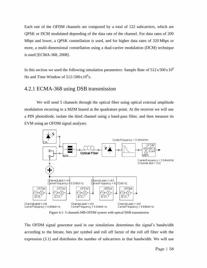
Page | 58
Each one of the OFDM channels are composed by a total of 122 subcarriers, which are
QPSK or DCM modulated depending of the data rate of the channel. For data rates of 200
Mbps and lower, a QPSK constellation is used, and for higher data rates of 320 Mbps or
more, a multi-dimensional constellation using a dual-carrier modulation (DCM) technique
is used [ECMA-368, 2008].
In this section we used the following simulation parameters: Sample Rate of 512 x 500 x 106
Hz and Time Window of 512 / 500 x 106
s.
4.2.1 ECMA-368 using DSB transmission
We will send 5 channels through the optical fiber using optical external amplitude
modulation recurring to a MZM biased at the quadrature point. At the receiver we will use
a PIN photodiode, isolate the third channel using a band-pass filter, and then measure its
EVM using an OFDM signal analyser.
Figure 4.1- 5 channels MB-OFDM system with optical DSB transmission
The OFDM signal generator used in our simulations determines the signal‟s bandwidth
according to the bitrate, bits per symbol and roll off factor of the roll off filter with the
expression (3.1) and distributes the number of subcarriers in that bandwidth. We will use
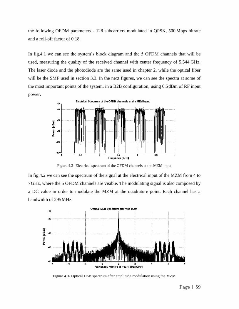
Page | 59
the following OFDM parameters - 128 subcarriers modulated in QPSK, 500 Mbps bitrate
and a roll-off factor of 0.18.
In fig.4.1 we can see the system‟s block diagram and the 5 OFDM channels that will be
used, measuring the quality of the received channel with center frequency of 5.544 GHz.
The laser diode and the photodiode are the same used in chapter 2, while the optical fiber
will be the SMF used in section 3.3. In the next figures, we can see the spectra at some of
the most important points of the system, in a B2B configuration, using 6.5 dBm of RF input
power.
Figure 4.2- Electrical spectrum of the OFDM channels at the MZM input
In fig.4.2 we can see the spectrum of the signal at the electrical input of the MZM from 4 to
7 GHz, where the 5 OFDM channels are visible. The modulating signal is also composed by
a DC value in order to modulate the MZM at the quadrature point. Each channel has a
bandwidth of 295 MHz.
Figure 4.3- Optical DSB spectrum after amplitude modulation using the MZM

Page | 60
Figure 4.4- Electrical spectrum of the 5 channels after PD
In fig 4.3 and 4.4, we can observe the spectra after the MZM and after PD. Then, the
channel at 5.544 GHz will be band-pass filtered in order to measure its EVM at the OFDM
analyzer. We obtained, once again, for 10 km of SMF, the optimal RF input power value of
6.5 dBm. Using this value, we traced the EVM versus fiber length curve of the 5.544 GHz
channel. From the results in fig.4.8 we can see that the channel‟s EVM is under the EVM
limit on the first 58 km.
4.2.2 ECMA-368 using VSB transmission
In this section, we will now use an optical filter after the MZM in order to generate
a VSB spectrum. With this modification we would avoid fading issues at the photodiode,
something that would be more relevant on the higher frequency channels like the ones
centered at 9.768 GHz and 10.296 GHz. We can see the system‟s block diagram in fig.4.5,
similar to the one in the last section, 3.2.1, except for the addition of the optical filter that
will suppress one of the optical sidebands.
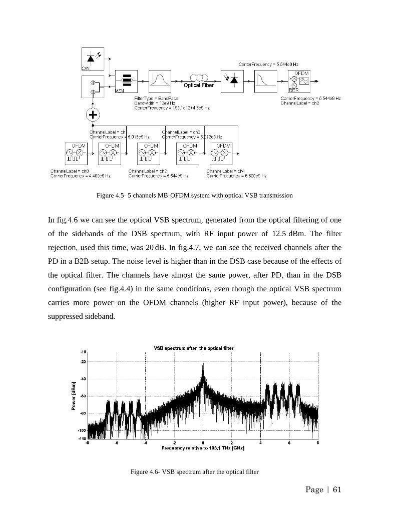
Page | 61
Figure 4.5- 5 channels MB-OFDM system with optical VSB transmission
In fig.4.6 we can see the optical VSB spectrum, generated from the optical filtering of one
of the sidebands of the DSB spectrum, with RF input power of 12.5 dBm. The filter
rejection, used this time, was 20 dB. In fig.4.7, we can see the received channels after the
PD in a B2B setup. The noise level is higher than in the DSB case because of the effects of
the optical filter. The channels have almost the same power, after PD, than in the DSB
configuration (see fig.4.4) in the same conditions, even though the optical VSB spectrum
carries more power on the OFDM channels (higher RF input power), because of the
suppressed sideband.
Figure 4.6- VSB spectrum after the optical filter
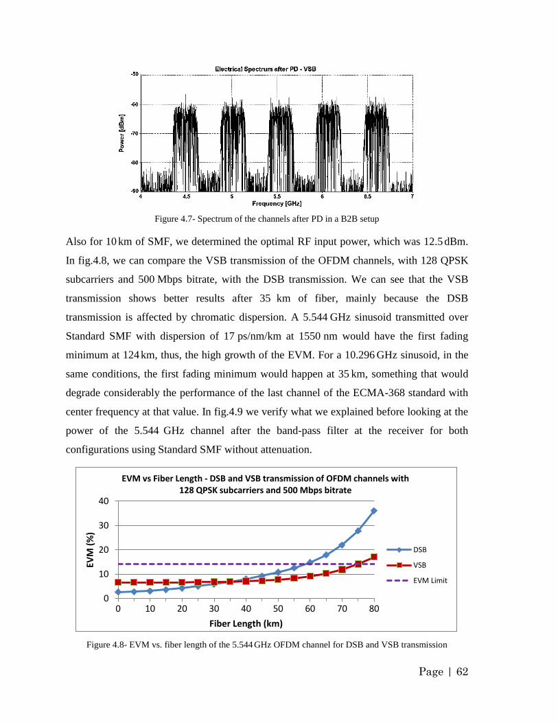
Page | 62
Figure 4.7- Spectrum of the channels after PD in a B2B setup
Also for 10 km of SMF, we determined the optimal RF input power, which was 12.5 dBm.
In fig.4.8, we can compare the VSB transmission of the OFDM channels, with 128 QPSK
subcarriers and 500 Mbps bitrate, with the DSB transmission. We can see that the VSB
transmission shows better results after 35 km of fiber, mainly because the DSB
transmission is affected by chromatic dispersion. A 5.544 GHz sinusoid transmitted over
Standard SMF with dispersion of 17 ps/nm/km at 1550 nm would have the first fading
minimum at 124 km, thus, the high growth of the EVM. For a 10.296 GHz sinusoid, in the
same conditions, the first fading minimum would happen at 35 km, something that would
degrade considerably the performance of the last channel of the ECMA-368 standard with
center frequency at that value. In fig.4.9 we verify what we explained before looking at the
power of the 5.544 GHz channel after the band-pass filter at the receiver for both
configurations using Standard SMF without attenuation.
Figure 4.8- EVM vs. fiber length of the 5.544 GHz OFDM channel for DSB and VSB transmission
0
10
20
30
40
0 10 20 30 40 50 60 70 80
EVM
(%
)
Fiber Length (km)
EVM vs Fiber Length - DSB and VSB transmission of OFDM channels with 128 QPSK subcarriers and 500 Mbps bitrate
DSB
VSB
EVM Limit
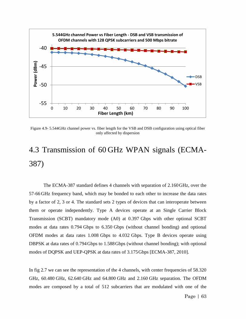
Page | 63
Figure 4.9- 5.544GHz channel power vs. fiber length for the VSB and DSB configuration using optical fiber
only affected by dispersion
4.3 Transmission of 60 GHz WPAN signals (ECMA-
387)
The ECMA-387 standard defines 4 channels with separation of 2.160 GHz, over the
57-66 GHz frequency band, which may be bonded to each other to increase the data rates
by a factor of 2, 3 or 4. The standard sets 2 types of devices that can interoperate between
them or operate independently. Type A devices operate at an Single Carrier Block
Transmission (SCBT) mandatory mode (A0) at 0.397 Gbps with other optional SCBT
modes at data rates 0.794 Gbps to 6.350 Gbps (without channel bonding) and optional
OFDM modes at data rates 1.008 Gbps to 4.032 Gbps. Type B devices operate using
DBPSK at data rates of 0.794 Gbps to 1.588 Gbps (without channel bonding); with optional
modes of DQPSK and UEP-QPSK at data rates of 3.175 Gbps [ECMA-387, 2010].
In fig 2.7 we can see the representation of the 4 channels, with center frequencies of 58.320
GHz, 60.480 GHz, 62.640 GHz and 64.800 GHz and 2.160 GHz separation. The OFDM
modes are composed by a total of 512 subcarriers that are modulated with one of the
-55
-50
-45
-40
0 10 20 30 40 50 60 70 80 90 100
Po
wer
(d
Bm
)
Fiber Length (km)
5.544GHz channel Power vs Fiber Length - DSB and VSB transmission of OFDM channels with 128 QPSK subcarriers and 500 Mbps bitrate
DSB
VSB
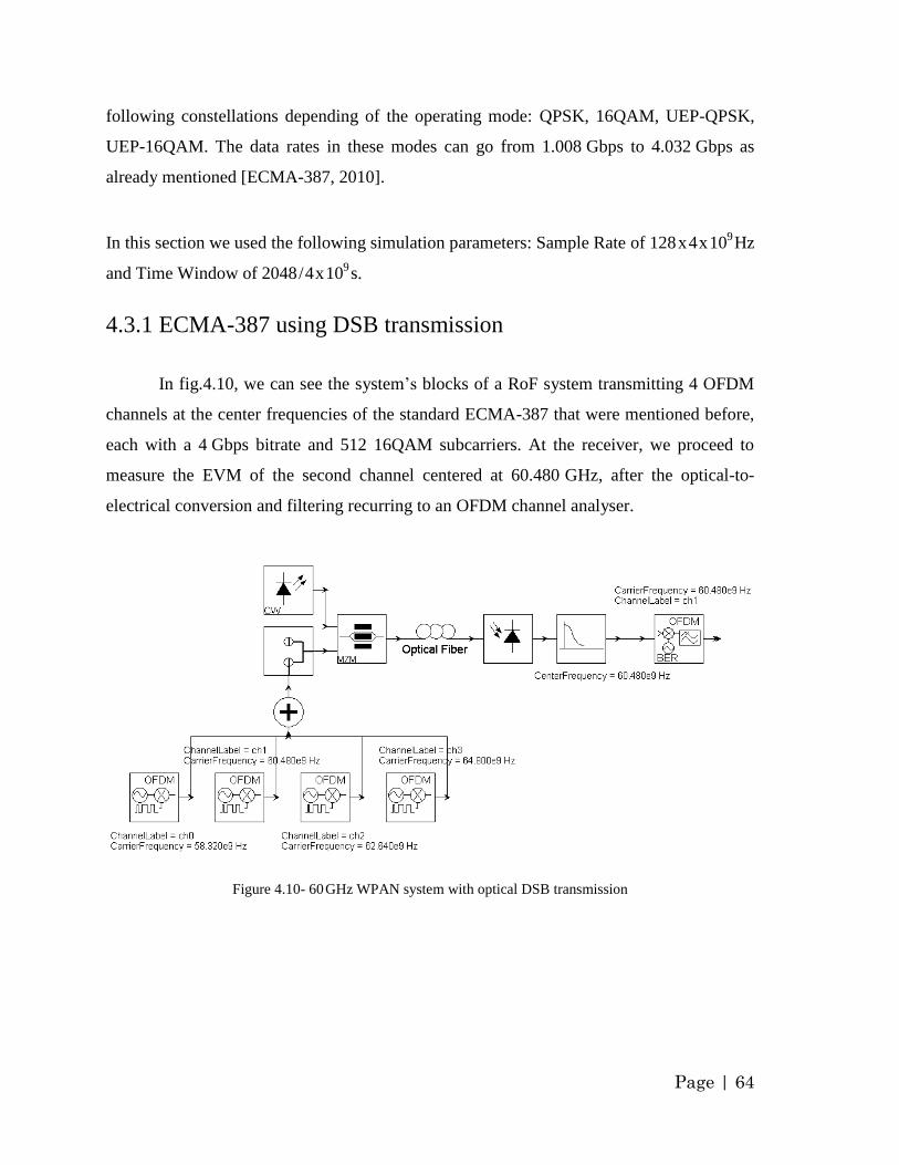
Page | 64
following constellations depending of the operating mode: QPSK, 16QAM, UEP-QPSK,
UEP-16QAM. The data rates in these modes can go from 1.008 Gbps to 4.032 Gbps as
already mentioned [ECMA-387, 2010].
In this section we used the following simulation parameters: Sample Rate of 128 x 4 x 109
Hz
and Time Window of 2048 / 4 x 10⁹
s.
4.3.1 ECMA-387 using DSB transmission
In fig.4.10, we can see the system‟s blocks of a RoF system transmitting 4 OFDM
channels at the center frequencies of the standard ECMA-387 that were mentioned before,
each with a 4 Gbps bitrate and 512 16QAM subcarriers. At the receiver, we proceed to
measure the EVM of the second channel centered at 60.480 GHz, after the optical-to-
electrical conversion and filtering recurring to an OFDM channel analyser.
Figure 4.10- 60 GHz WPAN system with optical DSB transmission
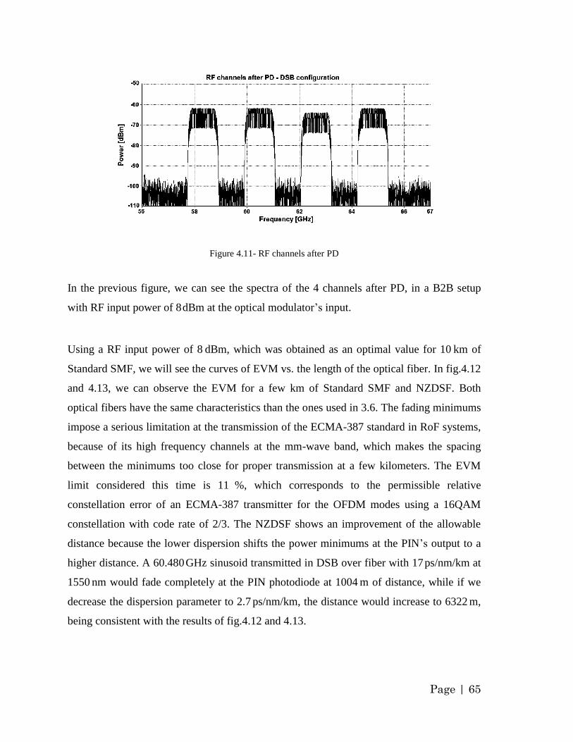
Page | 65
Figure 4.11- RF channels after PD
In the previous figure, we can see the spectra of the 4 channels after PD, in a B2B setup
with RF input power of 8 dBm at the optical modulator‟s input.
Using a RF input power of 8 dBm, which was obtained as an optimal value for 10 km of
Standard SMF, we will see the curves of EVM vs. the length of the optical fiber. In fig.4.12
and 4.13, we can observe the EVM for a few km of Standard SMF and NZDSF. Both
optical fibers have the same characteristics than the ones used in 3.6. The fading minimums
impose a serious limitation at the transmission of the ECMA-387 standard in RoF systems,
because of its high frequency channels at the mm-wave band, which makes the spacing
between the minimums too close for proper transmission at a few kilometers. The EVM
limit considered this time is 11 %, which corresponds to the permissible relative
constellation error of an ECMA-387 transmitter for the OFDM modes using a 16QAM
constellation with code rate of 2/3. The NZDSF shows an improvement of the allowable
distance because the lower dispersion shifts the power minimums at the PIN‟s output to a
higher distance. A 60.480 GHz sinusoid transmitted in DSB over fiber with 17 ps/nm/km at
1550 nm would fade completely at the PIN photodiode at 1004 m of distance, while if we
decrease the dispersion parameter to 2.7 ps/nm/km, the distance would increase to 6322 m,
being consistent with the results of fig.4.12 and 4.13.
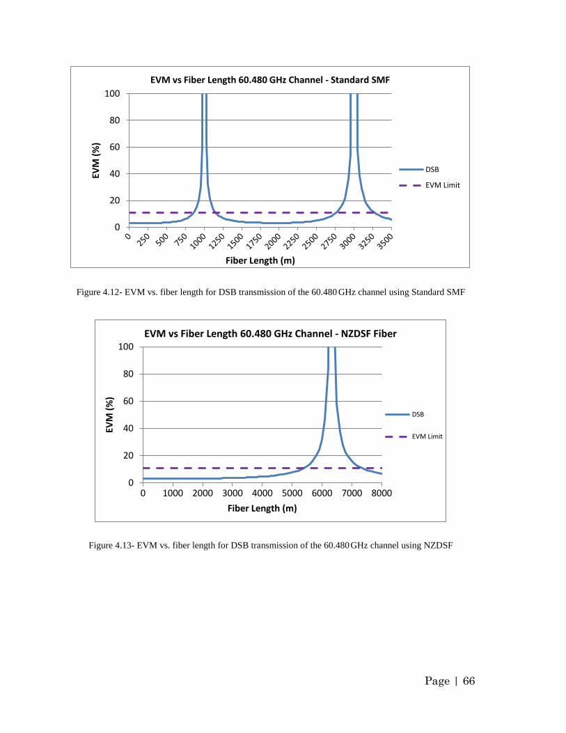
Page | 66
Figure 4.12- EVM vs. fiber length for DSB transmission of the 60.480 GHz channel using Standard SMF
Figure 4.13- EVM vs. fiber length for DSB transmission of the 60.480 GHz channel using NZDSF
0
20
40
60
80
100EV
M (
%)
Fiber Length (m)
EVM vs Fiber Length 60.480 GHz Channel - Standard SMF
DSB
EVM Limit
0
20
40
60
80
100
0 1000 2000 3000 4000 5000 6000 7000 8000
EVM
(%
)
Fiber Length (m)
EVM vs Fiber Length 60.480 GHz Channel - NZDSF Fiber
DSB
EVM Limit
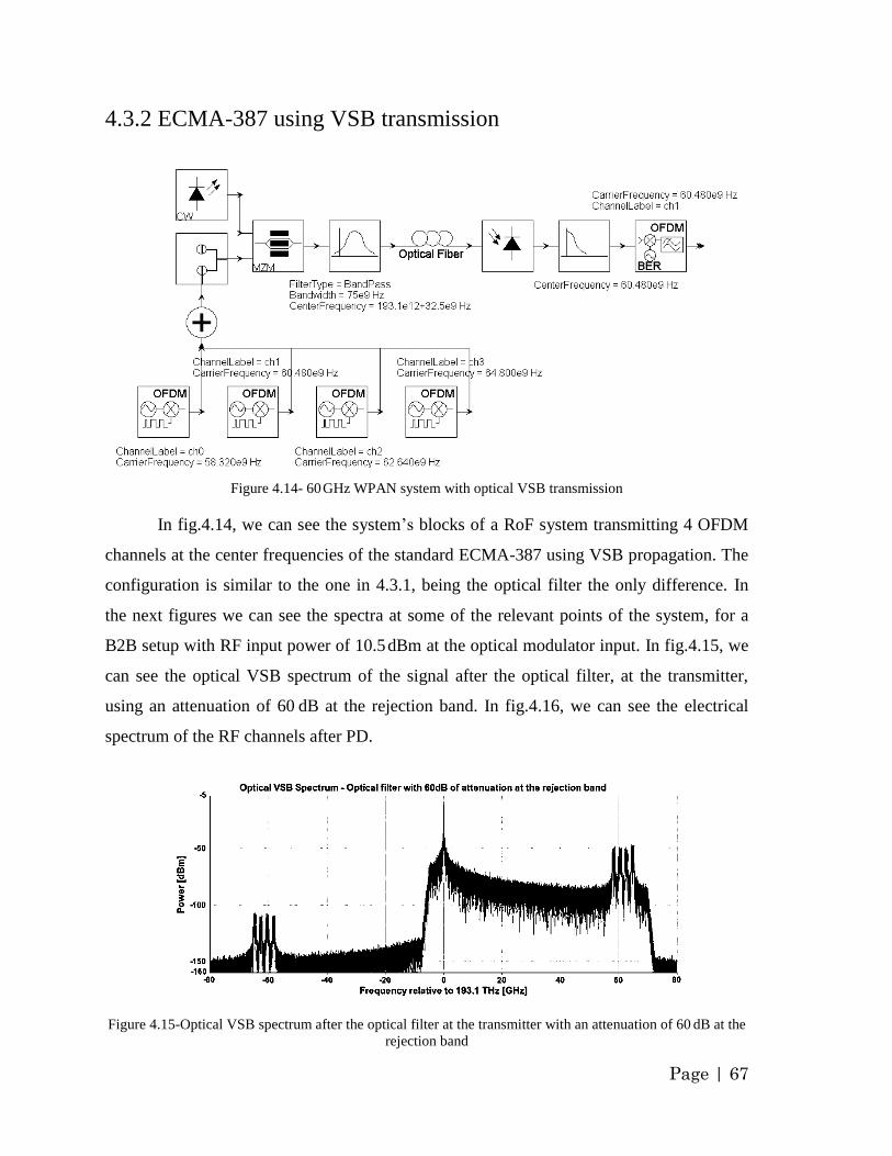
Page | 67
4.3.2 ECMA-387 using VSB transmission
Figure 4.14- 60 GHz WPAN system with optical VSB transmission
In fig.4.14, we can see the system‟s blocks of a RoF system transmitting 4 OFDM
channels at the center frequencies of the standard ECMA-387 using VSB propagation. The
configuration is similar to the one in 4.3.1, being the optical filter the only difference. In
the next figures we can see the spectra at some of the relevant points of the system, for a
B2B setup with RF input power of 10.5 dBm at the optical modulator input. In fig.4.15, we
can see the optical VSB spectrum of the signal after the optical filter, at the transmitter,
using an attenuation of 60 dB at the rejection band. In fig.4.16, we can see the electrical
spectrum of the RF channels after PD.
Figure 4.15-Optical VSB spectrum after the optical filter at the transmitter with an attenuation of 60 dB at the
rejection band
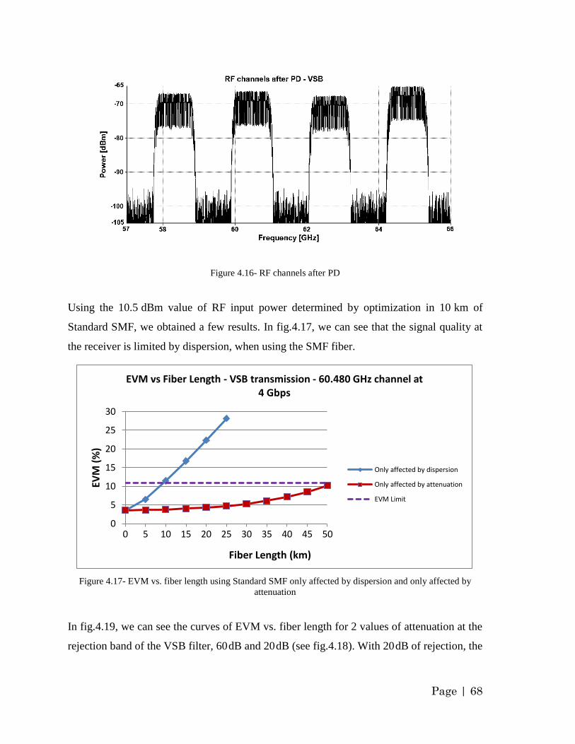
Page | 68
Figure 4.16- RF channels after PD
Using the 10.5 dBm value of RF input power determined by optimization in 10 km of
Standard SMF, we obtained a few results. In fig.4.17, we can see that the signal quality at
the receiver is limited by dispersion, when using the SMF fiber.
Figure 4.17- EVM vs. fiber length using Standard SMF only affected by dispersion and only affected by
attenuation
In fig.4.19, we can see the curves of EVM vs. fiber length for 2 values of attenuation at the
rejection band of the VSB filter, 60 dB and 20 dB (see fig.4.18). With 20 dB of rejection, the
0
5
10
15
20
25
30
0 5 10 15 20 25 30 35 40 45 50
EVM
(%
)
Fiber Length (km)
EVM vs Fiber Length - VSB transmission - 60.480 GHz channel at 4 Gbps
Only affected by dispersion
Only affected by attenuation
EVM Limit
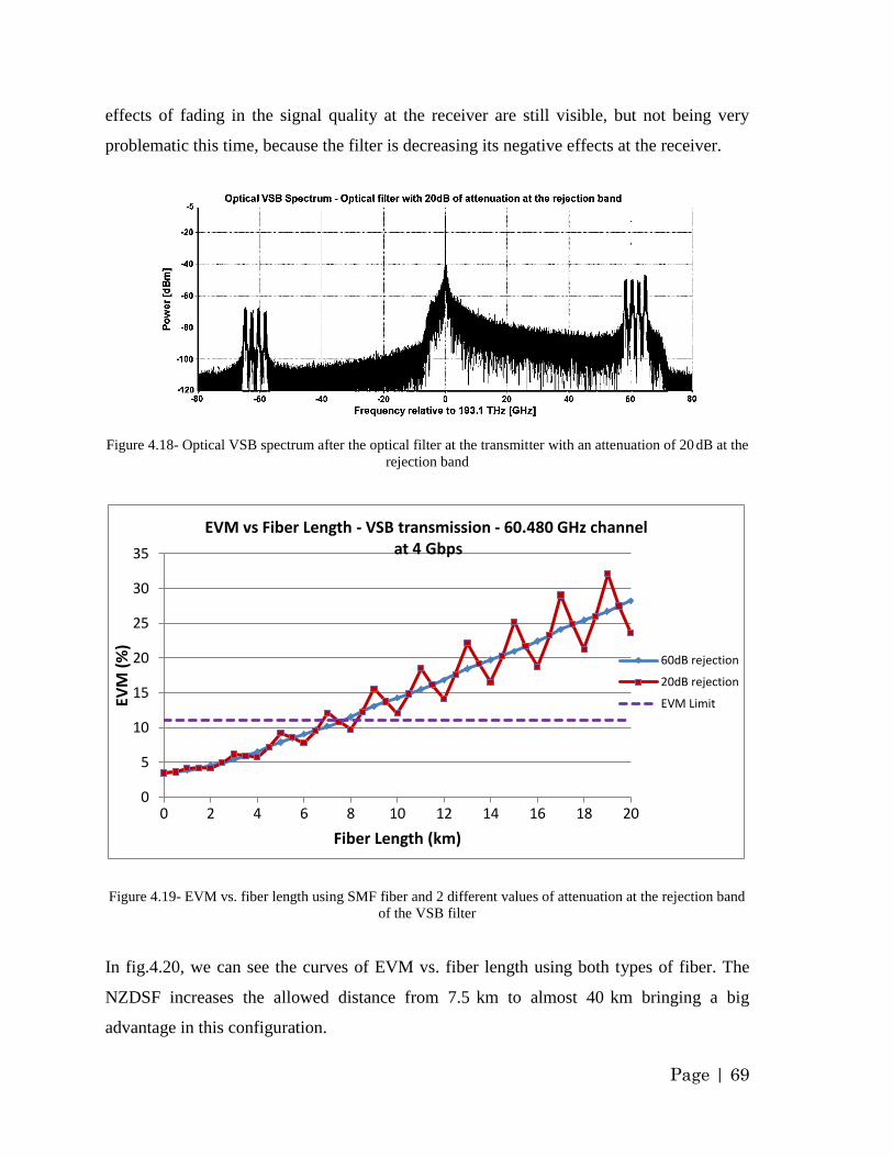
Page | 69
effects of fading in the signal quality at the receiver are still visible, but not being very
problematic this time, because the filter is decreasing its negative effects at the receiver.
Figure 4.18- Optical VSB spectrum after the optical filter at the transmitter with an attenuation of 20 dB at the
rejection band
Figure 4.19- EVM vs. fiber length using SMF fiber and 2 different values of attenuation at the rejection band
of the VSB filter
In fig.4.20, we can see the curves of EVM vs. fiber length using both types of fiber. The
NZDSF increases the allowed distance from 7.5 km to almost 40 km bringing a big
advantage in this configuration.
0
5
10
15
20
25
30
35
0 2 4 6 8 10 12 14 16 18 20
EVM
(%
)
Fiber Length (km)
EVM vs Fiber Length - VSB transmission - 60.480 GHz channel at 4 Gbps
60dB rejection
20dB rejection
EVM Limit
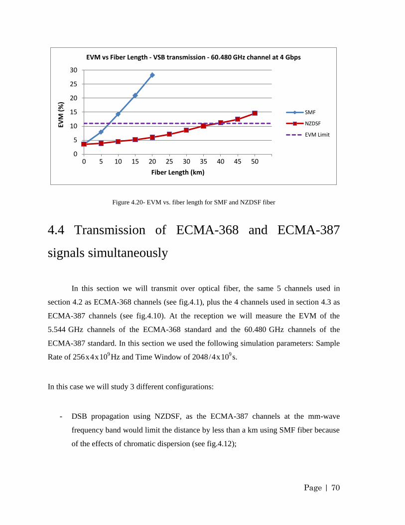
Page | 70
Figure 4.20- EVM vs. fiber length for SMF and NZDSF fiber
4.4 Transmission of ECMA-368 and ECMA-387
signals simultaneously
In this section we will transmit over optical fiber, the same 5 channels used in
section 4.2 as ECMA-368 channels (see fig.4.1), plus the 4 channels used in section 4.3 as
ECMA-387 channels (see fig.4.10). At the reception we will measure the EVM of the
5.544 GHz channels of the ECMA-368 standard and the 60.480 GHz channels of the
ECMA-387 standard. In this section we used the following simulation parameters: Sample
Rate of 256 x 4 x 109
Hz and Time Window of 2048 / 4 x 10⁹
s.
In this case we will study 3 different configurations:
- DSB propagation using NZDSF, as the ECMA-387 channels at the mm-wave
frequency band would limit the distance by less than a km using SMF fiber because
of the effects of chromatic dispersion (see fig.4.12);
0
5
10
15
20
25
30
0 5 10 15 20 25 30 35 40 45 50
EVM
(%
)
Fiber Length (km)
EVM vs Fiber Length - VSB transmission - 60.480 GHz channel at 4 Gbps
SMF
NZDSF
EVM Limit
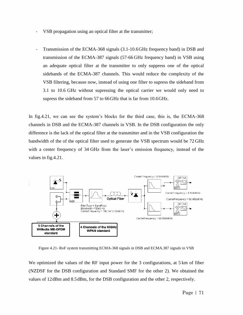
Page | 71
- VSB propagation using an optical filter at the transmitter;
- Transmission of the ECMA-368 signals (3.1-10.6 GHz frequency band) in DSB and
transmission of the ECMA-387 signals (57-66 GHz frequency band) in VSB using
an adequate optical filter at the transmitter to only suppress one of the optical
sidebands of the ECMA-387 channels. This would reduce the complexity of the
VSB filtering, because now, instead of using one filter to supress the sideband from
3.1 to 10.6 GHz without supressing the optical carrier we would only need to
supress the sideband from 57 to 66 GHz that is far from 10.6 GHz.
In fig.4.21, we can see the system‟s blocks for the third case, this is, the ECMA-368
channels in DSB and the ECMA-387 channels in VSB. In the DSB configuration the only
difference is the lack of the optical filter at the transmitter and in the VSB configuration the
bandwidth of the of the optical filter used to generate the VSB spectrum would be 72 GHz
with a center frequency of 34 GHz from the laser‟s emission frequency, instead of the
values in fig.4.21.
Figure 4.21- RoF system transmitting ECMA-368 signals in DSB and ECMA.387 signals in VSB
We optimized the values of the RF input power for the 3 configurations, at 5 km of fiber
(NZDSF for the DSB configuration and Standard SMF for the other 2). We obtained the
values of 12 dBm and 8.5 dBm, for the DSB configuration and the other 2, respectively.
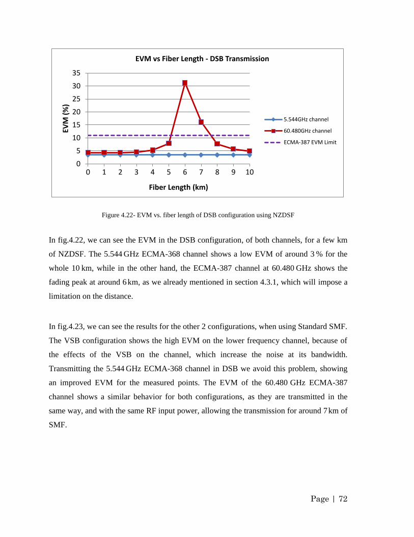
Page | 72
Figure 4.22- EVM vs. fiber length of DSB configuration using NZDSF
In fig.4.22, we can see the EVM in the DSB configuration, of both channels, for a few km
of NZDSF. The 5.544 GHz ECMA-368 channel shows a low EVM of around 3 % for the
whole 10 km, while in the other hand, the ECMA-387 channel at 60.480 GHz shows the
fading peak at around 6 km, as we already mentioned in section 4.3.1, which will impose a
limitation on the distance.
In fig.4.23, we can see the results for the other 2 configurations, when using Standard SMF.
The VSB configuration shows the high EVM on the lower frequency channel, because of
the effects of the VSB on the channel, which increase the noise at its bandwidth.
Transmitting the 5.544 GHz ECMA-368 channel in DSB we avoid this problem, showing
an improved EVM for the measured points. The EVM of the 60.480 GHz ECMA-387
channel shows a similar behavior for both configurations, as they are transmitted in the
same way, and with the same RF input power, allowing the transmission for around 7 km of
SMF.
0
5
10
15
20
25
30
35
0 1 2 3 4 5 6 7 8 9 10
EVM
(%
)
Fiber Length (km)
EVM vs Fiber Length - DSB Transmission
5.544GHz channel
60.480GHz channel
ECMA-387 EVM Limit
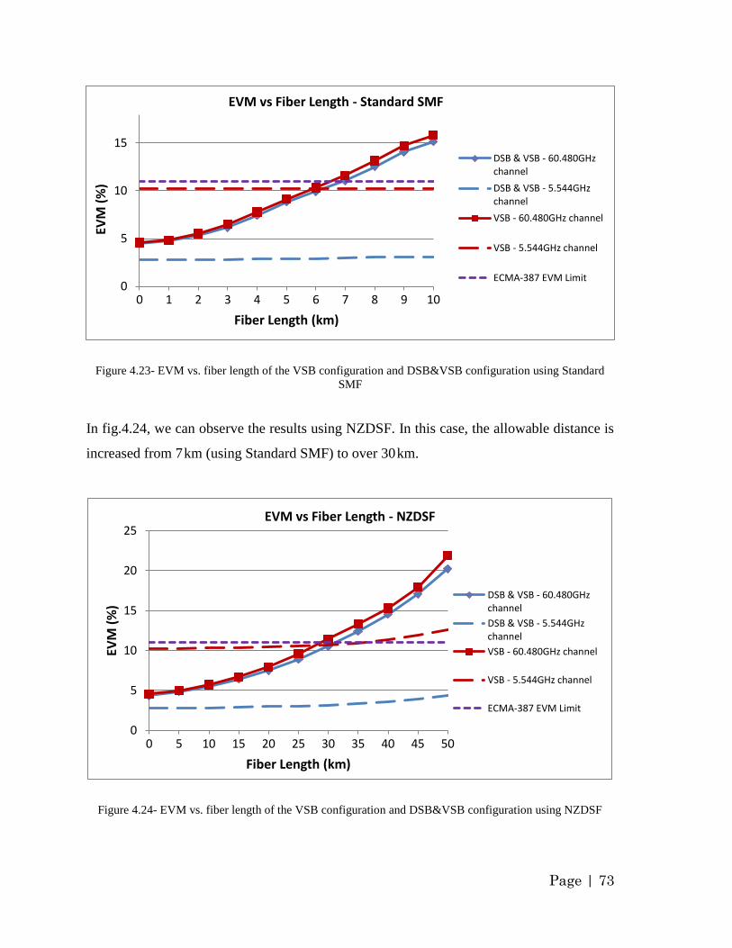
Page | 73
Figure 4.23- EVM vs. fiber length of the VSB configuration and DSB&VSB configuration using Standard
SMF
In fig.4.24, we can observe the results using NZDSF. In this case, the allowable distance is
increased from 7 km (using Standard SMF) to over 30 km.
Figure 4.24- EVM vs. fiber length of the VSB configuration and DSB&VSB configuration using NZDSF
0
5
10
15
0 1 2 3 4 5 6 7 8 9 10
EVM
(%
)
Fiber Length (km)
EVM vs Fiber Length - Standard SMF
DSB & VSB - 60.480GHzchannel
DSB & VSB - 5.544GHzchannel
VSB - 60.480GHz channel
VSB - 5.544GHz channel
ECMA-387 EVM Limit
0
5
10
15
20
25
0 5 10 15 20 25 30 35 40 45 50
EVM
(%
)
Fiber Length (km)
EVM vs Fiber Length - NZDSF
DSB & VSB - 60.480GHzchannel
DSB & VSB - 5.544GHzchannel
VSB - 60.480GHz channel
VSB - 5.544GHz channel
ECMA-387 EVM Limit
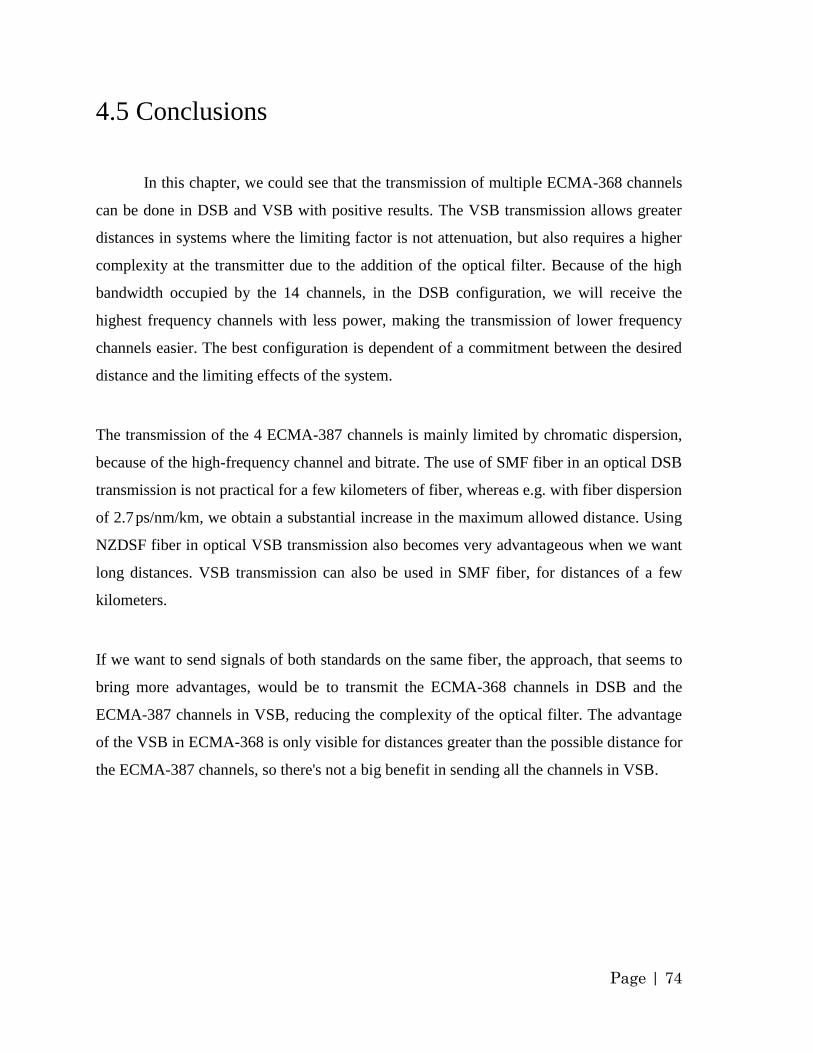
Page | 74
4.5 Conclusions
In this chapter, we could see that the transmission of multiple ECMA-368 channels
can be done in DSB and VSB with positive results. The VSB transmission allows greater
distances in systems where the limiting factor is not attenuation, but also requires a higher
complexity at the transmitter due to the addition of the optical filter. Because of the high
bandwidth occupied by the 14 channels, in the DSB configuration, we will receive the
highest frequency channels with less power, making the transmission of lower frequency
channels easier. The best configuration is dependent of a commitment between the desired
distance and the limiting effects of the system.
The transmission of the 4 ECMA-387 channels is mainly limited by chromatic dispersion,
because of the high-frequency channel and bitrate. The use of SMF fiber in an optical DSB
transmission is not practical for a few kilometers of fiber, whereas e.g. with fiber dispersion
of 2.7 ps/nm/km, we obtain a substantial increase in the maximum allowed distance. Using
NZDSF fiber in optical VSB transmission also becomes very advantageous when we want
long distances. VSB transmission can also be used in SMF fiber, for distances of a few
kilometers.
If we want to send signals of both standards on the same fiber, the approach, that seems to
bring more advantages, would be to transmit the ECMA-368 channels in DSB and the
ECMA-387 channels in VSB, reducing the complexity of the optical filter. The advantage
of the VSB in ECMA-368 is only visible for distances greater than the possible distance for
the ECMA-387 channels, so there's not a big benefit in sending all the channels in VSB.
Page | 75
Chapter 5. Distribution of digital video signals over
optical fiber
5.1 Introduction
In this chapter we will evaluate the performance, by simulation, of a
digital video transmission system over optical fiber recurring, once again, to the software
VPITransmissionMaker™. We will proceed to the transmission of several channels,
modelled in accordance to some of the digital video broadcasting standards presented in
chapter 2, this is, DVB-C, DVB-T and DVB-S. The digital channels will be transmitted
over the analog fiber-optic link using external modulation, which has shown improvements
in terms of noise figure and spurious-free dynamic range (SFDR) over direct modulation
[Karim, 2007]. The wavelength used in this case 1554vnm, which allows low attenuation
and the use of optical amplifiers. The use of optical amplifiers makes 1550 nm technology
economically viable. The inherently slow gain medium in erbium-doped or erbium-
ytterbium co-doped optical amplifiers makes distortion from gain-saturation effects
virtually negligible at the CATV frequencies, which are also used in digital TV
broadcasting [Phillips, 1998].
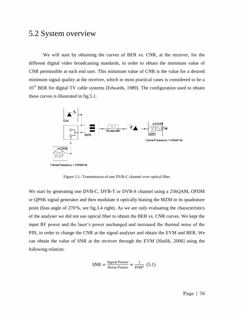
Page | 76
5.2 System overview
We will start by obtaining the curves of BER vs. CNR, at the receiver, for the
different digital video broadcasting standards, in order to obtain the minimum value of
CNR permissible at each end user. This minimum value of CNR is the value for a desired
minimum signal quality at the receiver, which in most practical cases is considered to be a
10-6
BER for digital TV cable systems [Edwards, 1989]. The configuration used to obtain
these curves is illustrated in fig.5.1.
Figure 5.1- Transmission of one DVB-C channel over optical fiber
We start by generating one DVB-C, DVB-T or DVB-S channel using a 256QAM, OFDM
or QPSK signal generator and then modulate it optically biasing the MZM in its quadrature
point (bias angle of 270 %, see fig.3.4 right). As we are only evaluating the characteristics
of the analyser we did not use optical fiber to obtain the BER vs. CNR curves. We kept the
input RF power and the laser‟s power unchanged and increased the thermal noise of the
PIN, in order to change the CNR at the signal analyser and obtain the EVM and BER. We
can obtain the value of SNR at the receiver through the EVM [Shafik, 2006] using the
following relation:
(5.1)
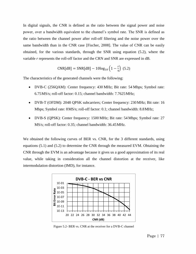
Page | 77
In digital signals, the CNR is defined as the ratio between the signal power and noise
power, over a bandwidth equivalent to the channel‟s symbol rate. The SNR is defined as
the ratio between the channel power after roll-off filtering and the noise power over the
same bandwidth than in the CNR case [Fischer, 2008]. The value of CNR can be easily
obtained, for the various standards, through the SNR using equation (5.2), where the
variable r represents the roll-off factor and the CRN and SNR are expressed in dB.
(
) (5.2)
The characteristics of the generated channels were the following:
DVB-C (256QAM): Center frequency: 430 MHz; Bit rate: 54 Mbps; Symbol rate:
6.75 MS/s; roll-off factor: 0.15; channel bandwidth: 7.7625 MHz;
DVB-T (OFDM): 2048 QPSK subcarriers; Center frequency: 230 MHz; Bit rate: 16
Mbps; Symbol rate: 8 MS/s; roll-off factor: 0.1; channel bandwidth: 8.8 MHz;
DVB-S (QPSK): Center frequency: 1500 MHz; Bit rate: 54 Mbps; Symbol rate: 27
MS/s; roll-off factor: 0.35; channel bandwidth: 36.45 MHz.
We obtained the following curves of BER vs. CNR, for the 3 different standards, using
equations (5.1) and (5.2) to determine the CNR through the measured EVM. Obtaining the
CNR through the EVM is an advantage because it gives us a good approximation of its real
value, while taking in consideration all the channel distortion at the receiver, like
intermodulation distortion (IMD), for instance.
Figure 5.2- BER vs. CNR at the receiver for a DVB-C channel
1E-13
1E-11
1E-09
1E-07
1E-05
1E-03
1E-01
20 22 24 26 28 30 32 34 36 38 40 42 44
Bit
Err
or
Rat
e
CNR (dB)
DVB-C - BER vs CNR
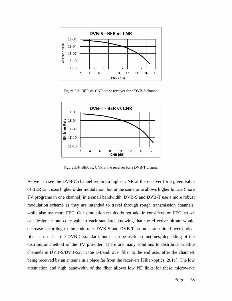
Page | 78
Figure 5.3- BER vs. CNR at the receiver for a DVB-S channel
Figure 5.4- BER vs. CNR at the receiver for a DVB-T channel
As we can see the DVB-C channel require a higher CNR at the receiver for a given value
of BER as it uses higher order modulation, but at the same time allows higher bitrate (more
TV programs in one channel) in a small bandwidth. DVB-S and DVB-T use a more robust
modulation scheme as they are intended to travel through rough transmission channels,
while also use more FEC. Our simulation results do not take in consideration FEC, so we
can designate one code gain to each standard, knowing that the effective bitrate would
decrease according to the code rate. DVB-S and DVB-T are not transmitted over optical
fiber as usual as the DVB-C standard, but it can be useful sometimes, depending of the
distribution method of the TV provider. There are many solutions to distribute satellite
channels in DVB-S/DVB-S2, in the L-Band, over fiber to the end user, after the channels
being received by an antenna in a place far from the receivers [Fiber-optics, 2011]. The low
attenuation and high bandwidth of the fiber allows low NF links for these microwave
1E-13
1E-10
1E-07
1E-04
1E-01
2 4 6 8 10 12 14 16 18
Bit
Err
or
Rat
e
CNR (dB)
DVB-S - BER vs CNR
1E-13
1E-10
1E-07
1E-04
1E-01
2 4 6 8 10 12 14 16
Bit
Err
or
Rat
e
CNR (dB)
DVB-T - BER vs CNR
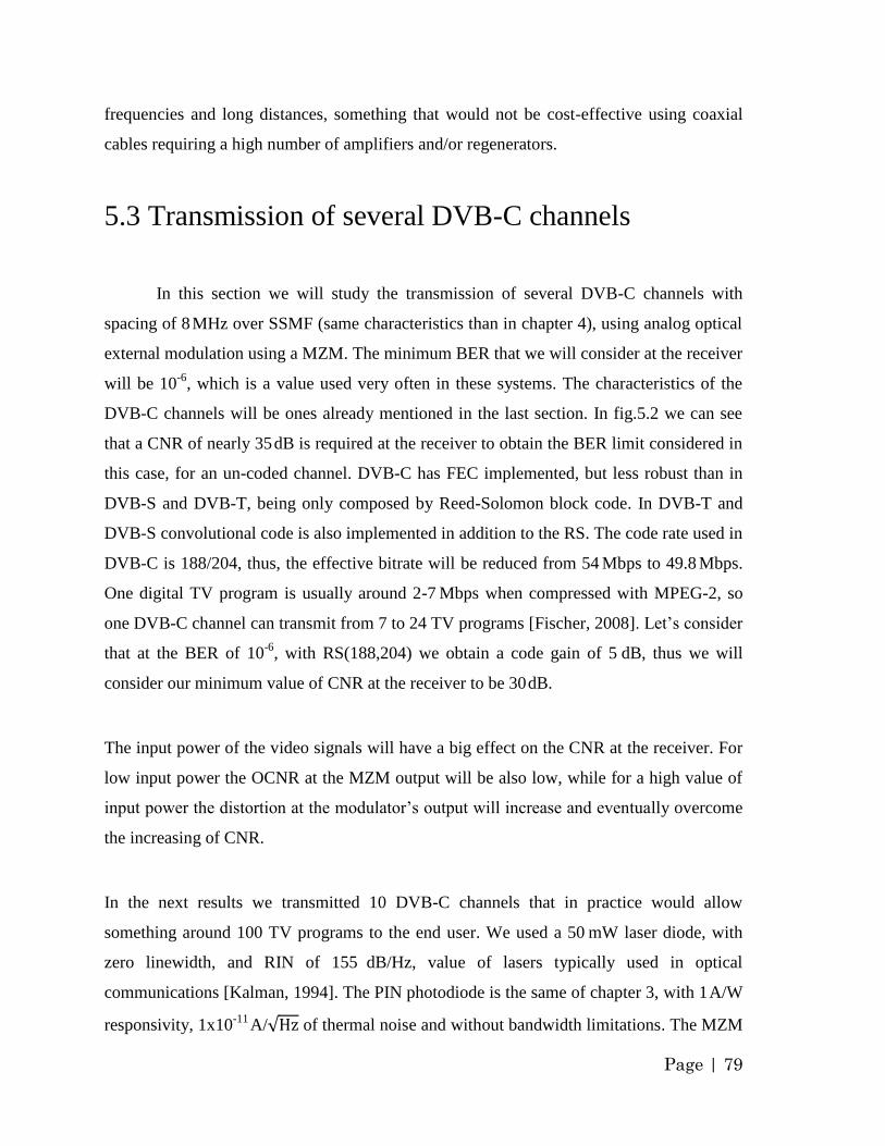
Page | 79
frequencies and long distances, something that would not be cost-effective using coaxial
cables requiring a high number of amplifiers and/or regenerators.
5.3 Transmission of several DVB-C channels
In this section we will study the transmission of several DVB-C channels with
spacing of 8 MHz over SSMF (same characteristics than in chapter 4), using analog optical
external modulation using a MZM. The minimum BER that we will consider at the receiver
will be 10-6
, which is a value used very often in these systems. The characteristics of the
DVB-C channels will be ones already mentioned in the last section. In fig.5.2 we can see
that a CNR of nearly 35 dB is required at the receiver to obtain the BER limit considered in
this case, for an un-coded channel. DVB-C has FEC implemented, but less robust than in
DVB-S and DVB-T, being only composed by Reed-Solomon block code. In DVB-T and
DVB-S convolutional code is also implemented in addition to the RS. The code rate used in
DVB-C is 188/204, thus, the effective bitrate will be reduced from 54 Mbps to 49.8 Mbps.
One digital TV program is usually around 2-7 Mbps when compressed with MPEG-2, so
one DVB-C channel can transmit from 7 to 24 TV programs [Fischer, 2008]. Let‟s consider
that at the BER of 10-6
, with RS(188,204) we obtain a code gain of 5 dB, thus we will
consider our minimum value of CNR at the receiver to be 30 dB.
The input power of the video signals will have a big effect on the CNR at the receiver. For
low input power the OCNR at the MZM output will be also low, while for a high value of
input power the distortion at the modulator‟s output will increase and eventually overcome
the increasing of CNR.
In the next results we transmitted 10 DVB-C channels that in practice would allow
something around 100 TV programs to the end user. We used a 50 mW laser diode, with
zero linewidth, and RIN of 155 dB/Hz, value of lasers typically used in optical
communications [Kalman, 1994]. The PIN photodiode is the same of chapter 3, with 1 A/W
responsivity, 1x10-11
A/√ of thermal noise and without bandwidth limitations. The MZM
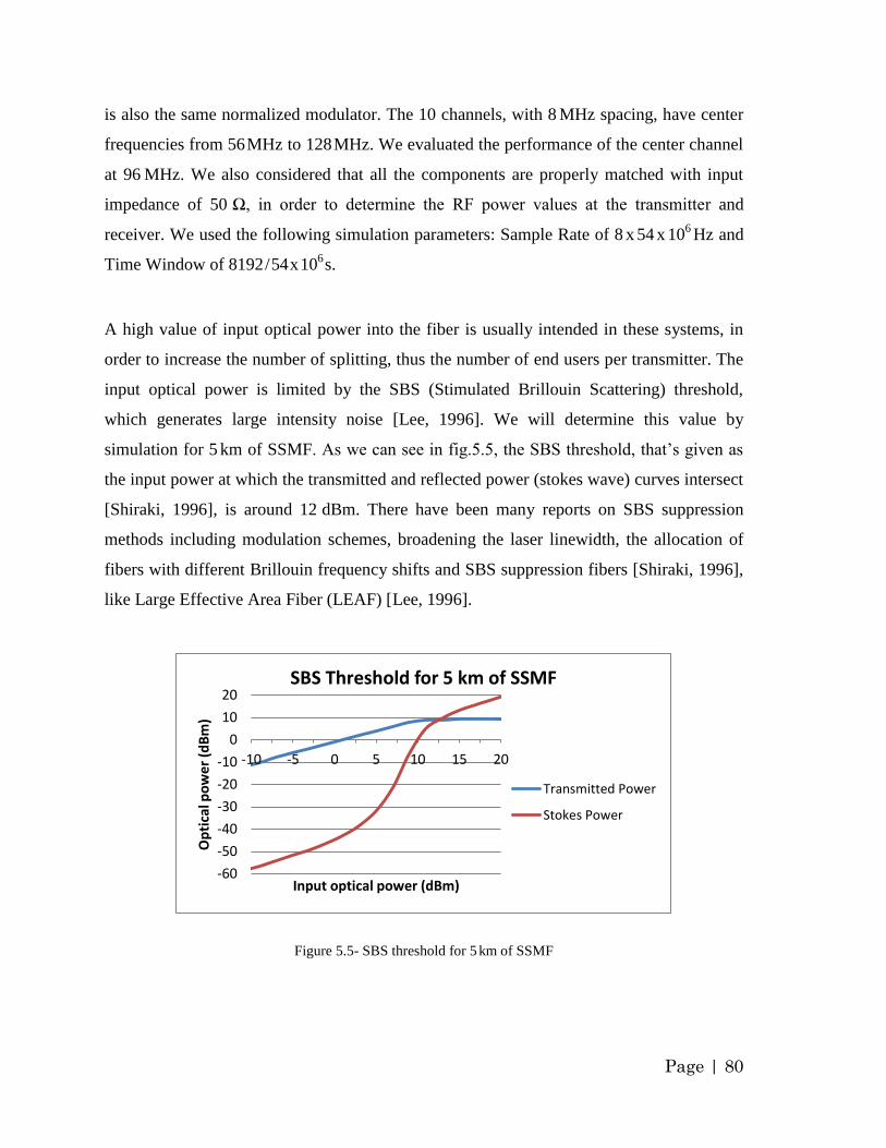
Page | 80
is also the same normalized modulator. The 10 channels, with 8 MHz spacing, have center
frequencies from 56 MHz to 128 MHz. We evaluated the performance of the center channel
at 96 MHz. We also considered that all the components are properly matched with input
impedance of 50 Ω, in order to determine the RF power values at the transmitter and
receiver. We used the following simulation parameters: Sample Rate of 8 x 54 x 106
Hz and
Time Window of 8192 / 54 x 106 s.
A high value of input optical power into the fiber is usually intended in these systems, in
order to increase the number of splitting, thus the number of end users per transmitter. The
input optical power is limited by the SBS (Stimulated Brillouin Scattering) threshold,
which generates large intensity noise [Lee, 1996]. We will determine this value by
simulation for 5 km of SSMF. As we can see in fig.5.5, the SBS threshold, that‟s given as
the input power at which the transmitted and reflected power (stokes wave) curves intersect
[Shiraki, 1996], is around 12 dBm. There have been many reports on SBS suppression
methods including modulation schemes, broadening the laser linewidth, the allocation of
fibers with different Brillouin frequency shifts and SBS suppression fibers [Shiraki, 1996],
like Large Effective Area Fiber (LEAF) [Lee, 1996].
Figure 5.5- SBS threshold for 5 km of SSMF
-60
-50
-40
-30
-20
-10
0
10
20
-10 -5 0 5 10 15 20
Op
tica
l po
wer
(d
Bm
)
Input optical power (dBm)
SBS Threshold for 5 km of SSMF
Transmitted Power
Stokes Power
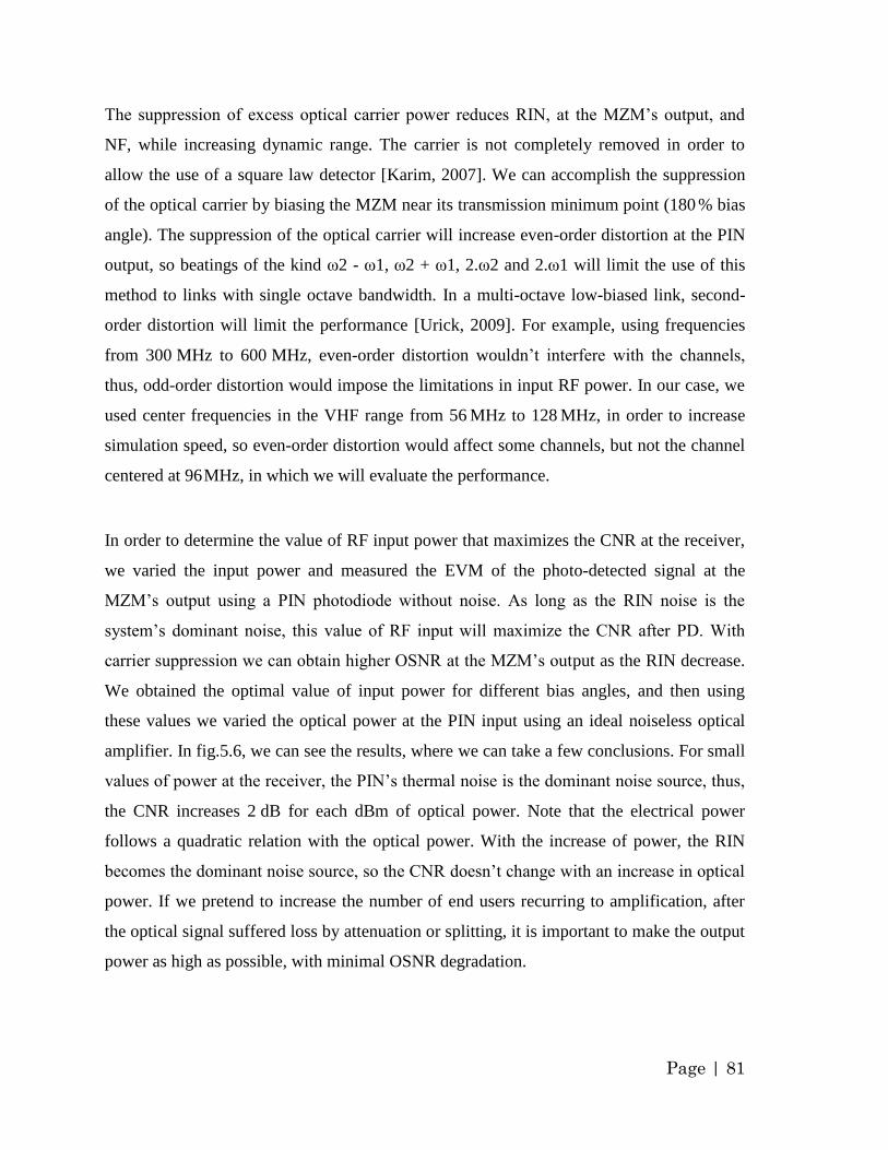
Page | 81
The suppression of excess optical carrier power reduces RIN, at the MZM‟s output, and
NF, while increasing dynamic range. The carrier is not completely removed in order to
allow the use of a square law detector [Karim, 2007]. We can accomplish the suppression
of the optical carrier by biasing the MZM near its transmission minimum point (180 % bias
angle). The suppression of the optical carrier will increase even-order distortion at the PIN
output, so beatings of the kind ω2 - ω1, ω2 + ω1, 2.ω2 and 2.ω1 will limit the use of this
method to links with single octave bandwidth. In a multi-octave low-biased link, second-
order distortion will limit the performance [Urick, 2009]. For example, using frequencies
from 300 MHz to 600 MHz, even-order distortion wouldn‟t interfere with the channels,
thus, odd-order distortion would impose the limitations in input RF power. In our case, we
used center frequencies in the VHF range from 56 MHz to 128 MHz, in order to increase
simulation speed, so even-order distortion would affect some channels, but not the channel
centered at 96 MHz, in which we will evaluate the performance.
In order to determine the value of RF input power that maximizes the CNR at the receiver,
we varied the input power and measured the EVM of the photo-detected signal at the
MZM‟s output using a PIN photodiode without noise. As long as the RIN noise is the
system‟s dominant noise, this value of RF input will maximize the CNR after PD. With
carrier suppression we can obtain higher OSNR at the MZM‟s output as the RIN decrease.
We obtained the optimal value of input power for different bias angles, and then using
these values we varied the optical power at the PIN input using an ideal noiseless optical
amplifier. In fig.5.6, we can see the results, where we can take a few conclusions. For small
values of power at the receiver, the PIN‟s thermal noise is the dominant noise source, thus,
the CNR increases 2 dB for each dBm of optical power. Note that the electrical power
follows a quadratic relation with the optical power. With the increase of power, the RIN
becomes the dominant noise source, so the CNR doesn‟t change with an increase in optical
power. If we pretend to increase the number of end users recurring to amplification, after
the optical signal suffered loss by attenuation or splitting, it is important to make the output
power as high as possible, with minimal OSNR degradation.
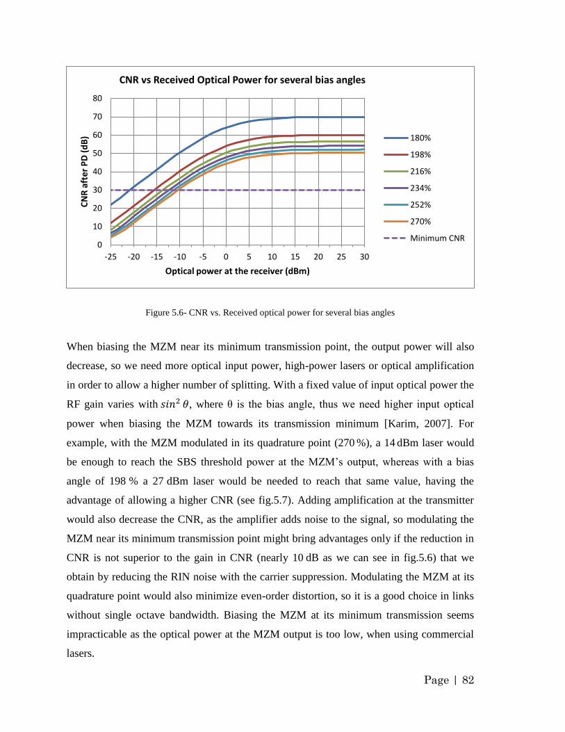
Page | 82
Figure 5.6- CNR vs. Received optical power for several bias angles
When biasing the MZM near its minimum transmission point, the output power will also
decrease, so we need more optical input power, high-power lasers or optical amplification
in order to allow a higher number of splitting. With a fixed value of input optical power the
RF gain varies with , where θ is the bias angle, thus we need higher input optical
power when biasing the MZM towards its transmission minimum [Karim, 2007]. For
example, with the MZM modulated in its quadrature point (270 %), a 14 dBm laser would
be enough to reach the SBS threshold power at the MZM‟s output, whereas with a bias
angle of 198 % a 27 dBm laser would be needed to reach that same value, having the
advantage of allowing a higher CNR (see fig.5.7). Adding amplification at the transmitter
would also decrease the CNR, as the amplifier adds noise to the signal, so modulating the
MZM near its minimum transmission point might bring advantages only if the reduction in
CNR is not superior to the gain in CNR (nearly 10 dB as we can see in fig.5.6) that we
obtain by reducing the RIN noise with the carrier suppression. Modulating the MZM at its
quadrature point would also minimize even-order distortion, so it is a good choice in links
without single octave bandwidth. Biasing the MZM at its minimum transmission seems
impracticable as the optical power at the MZM output is too low, when using commercial
lasers.
0
10
20
30
40
50
60
70
80
-25 -20 -15 -10 -5 0 5 10 15 20 25 30
CN
R a
fte
r P
D (
dB
)
Optical power at the receiver (dBm)
CNR vs Received Optical Power for several bias angles
180%
198%
216%
234%
252%
270%
Minimum CNR
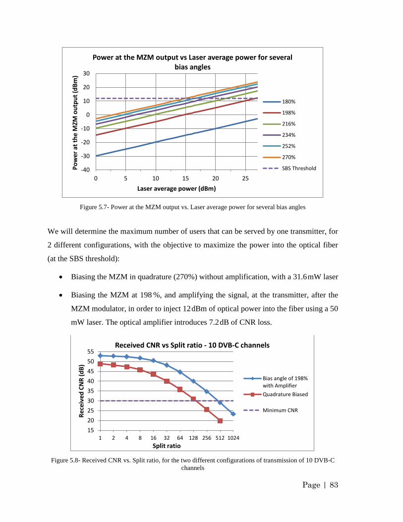
Page | 83
Figure 5.7- Power at the MZM output vs. Laser average power for several bias angles
We will determine the maximum number of users that can be served by one transmitter, for
2 different configurations, with the objective to maximize the power into the optical fiber
(at the SBS threshold):
Biasing the MZM in quadrature (270%) without amplification, with a 31.6 mW laser
Biasing the MZM at 198 %, and amplifying the signal, at the transmitter, after the
MZM modulator, in order to inject 12 dBm of optical power into the fiber using a 50
mW laser. The optical amplifier introduces 7.2 dB of CNR loss.
Figure 5.8- Received CNR vs. Split ratio, for the two different configurations of transmission of 10 DVB-C
channels
-40
-30
-20
-10
0
10
20
30
0 5 10 15 20 25
Po
we
r at
th
e M
ZM o
utp
ut
(dB
m)
Laser average power (dBm)
Power at the MZM output vs Laser average power for several bias angles
180%
198%
216%
234%
252%
270%
SBS Threshold
15
20
25
30
35
40
45
50
55
1 2 4 8 16 32 64 128 256 512 1024
Rec
eiv
ed C
NR
(d
B)
Split ratio
Received CNR vs Split ratio - 10 DVB-C channels
Bias angle of 198%with Amplifier
Quadrature Biased
Minimum CNR
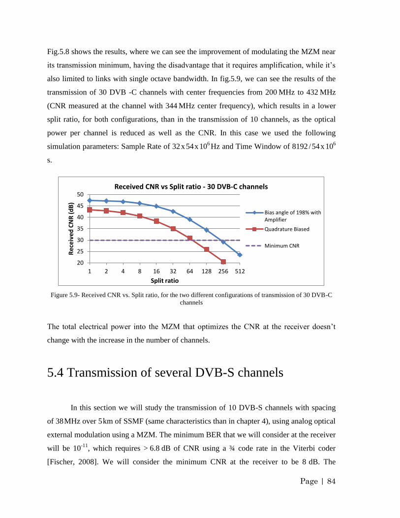
Page | 84
Fig.5.8 shows the results, where we can see the improvement of modulating the MZM near
its transmission minimum, having the disadvantage that it requires amplification, while it‟s
also limited to links with single octave bandwidth. In fig.5.9, we can see the results of the
transmission of 30 DVB -C channels with center frequencies from 200 MHz to 432 MHz
(CNR measured at the channel with 344 MHz center frequency), which results in a lower
split ratio, for both configurations, than in the transmission of 10 channels, as the optical
power per channel is reduced as well as the CNR. In this case we used the following
simulation parameters: Sample Rate of 32 x 54 x 106
Hz and Time Window of 8192 / 54 x 106
s.
Figure 5.9- Received CNR vs. Split ratio, for the two different configurations of transmission of 30 DVB-C
channels
The total electrical power into the MZM that optimizes the CNR at the receiver doesn‟t
change with the increase in the number of channels.
5.4 Transmission of several DVB-S channels
In this section we will study the transmission of 10 DVB-S channels with spacing
of 38 MHz over 5 km of SSMF (same characteristics than in chapter 4), using analog optical
external modulation using a MZM. The minimum BER that we will consider at the receiver
will be 10-11
, which requires > 6.8 dB of CNR using a ¾ code rate in the Viterbi coder
[Fischer, 2008]. We will consider the minimum CNR at the receiver to be 8 dB. The
20
25
30
35
40
45
50
1 2 4 8 16 32 64 128 256 512
Rec
eiv
ed C
NR
(d
B)
Split ratio
Received CNR vs Split ratio - 30 DVB-C channels
Bias angle of 198% withAmplifier
Quadrature Biased
Minimum CNR
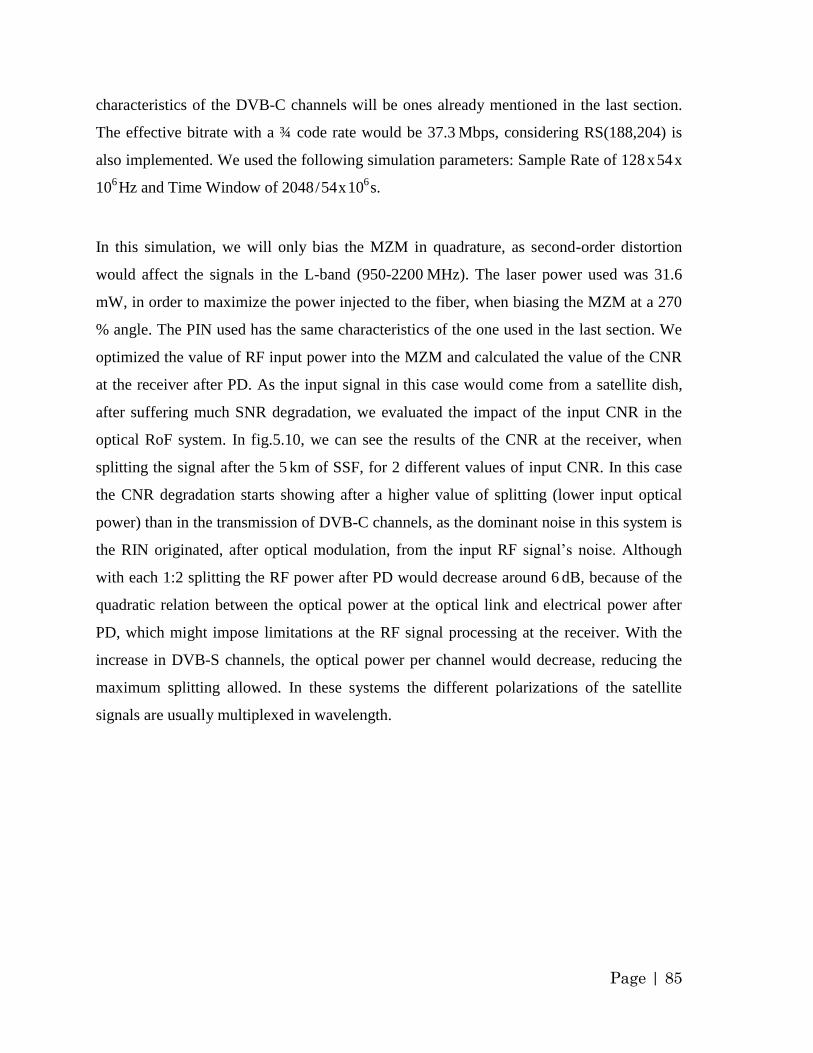
Page | 85
characteristics of the DVB-C channels will be ones already mentioned in the last section.
The effective bitrate with a ¾ code rate would be 37.3 Mbps, considering RS(188,204) is
also implemented. We used the following simulation parameters: Sample Rate of 128 x 54 x
106
Hz and Time Window of 2048 / 54 x 106 s.
In this simulation, we will only bias the MZM in quadrature, as second-order distortion
would affect the signals in the L-band (950-2200 MHz). The laser power used was 31.6
mW, in order to maximize the power injected to the fiber, when biasing the MZM at a 270
% angle. The PIN used has the same characteristics of the one used in the last section. We
optimized the value of RF input power into the MZM and calculated the value of the CNR
at the receiver after PD. As the input signal in this case would come from a satellite dish,
after suffering much SNR degradation, we evaluated the impact of the input CNR in the
optical RoF system. In fig.5.10, we can see the results of the CNR at the receiver, when
splitting the signal after the 5 km of SSF, for 2 different values of input CNR. In this case
the CNR degradation starts showing after a higher value of splitting (lower input optical
power) than in the transmission of DVB-C channels, as the dominant noise in this system is
the RIN originated, after optical modulation, from the input RF signal‟s noise. Although
with each 1:2 splitting the RF power after PD would decrease around 6 dB, because of the
quadratic relation between the optical power at the optical link and electrical power after
PD, which might impose limitations at the RF signal processing at the receiver. With the
increase in DVB-S channels, the optical power per channel would decrease, reducing the
maximum splitting allowed. In these systems the different polarizations of the satellite
signals are usually multiplexed in wavelength.
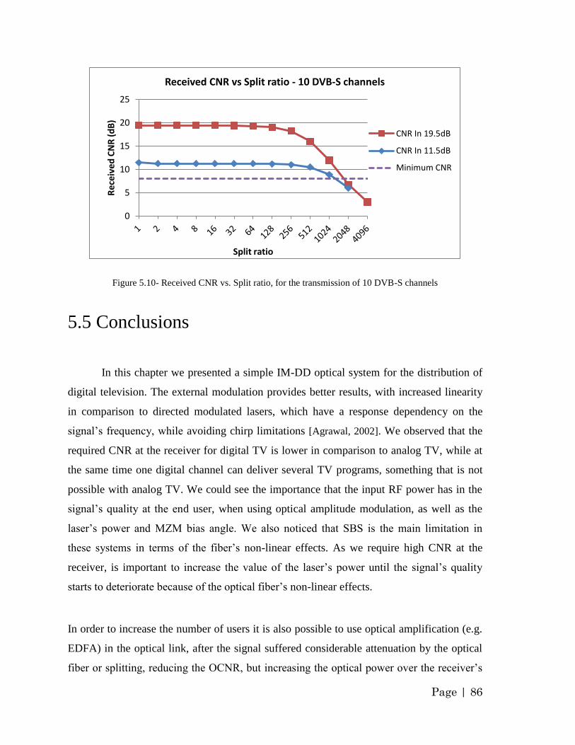
Page | 86
Figure 5.10- Received CNR vs. Split ratio, for the transmission of 10 DVB-S channels
5.5 Conclusions
In this chapter we presented a simple IM-DD optical system for the distribution of
digital television. The external modulation provides better results, with increased linearity
in comparison to directed modulated lasers, which have a response dependency on the
signal‟s frequency, while avoiding chirp limitations [Agrawal, 2002]. We observed that the
required CNR at the receiver for digital TV is lower in comparison to analog TV, while at
the same time one digital channel can deliver several TV programs, something that is not
possible with analog TV. We could see the importance that the input RF power has in the
signal‟s quality at the end user, when using optical amplitude modulation, as well as the
laser‟s power and MZM bias angle. We also noticed that SBS is the main limitation in
these systems in terms of the fiber‟s non-linear effects. As we require high CNR at the
receiver, is important to increase the value of the laser‟s power until the signal‟s quality
starts to deteriorate because of the optical fiber‟s non-linear effects.
In order to increase the number of users it is also possible to use optical amplification (e.g.
EDFA) in the optical link, after the signal suffered considerable attenuation by the optical
fiber or splitting, reducing the OCNR, but increasing the optical power over the receiver‟s
0
5
10
15
20
25R
ece
ive
d C
NR
(d
B)
Split ratio
Received CNR vs Split ratio - 10 DVB-S channels
CNR In 19.5dB
CNR In 11.5dB
Minimum CNR
Page | 87
sensitivity. Reducing the laser‟s RIN, allows us a higher OCNR at the transmitter so it‟s
always an important parameter to consider in the implementation of analog fiber links. We
could also verify by simulation, that modulating the MZM near its transmission minimum,
reducing the carrier‟s power, allow us to have higher values of OCNR at the transmitter,
with the main disadvantages of increasing second-order distortion at the PD (limiting its
use to single octave bandwidth links), and requiring amplification at the transmitter in order
to maximize the optical power launched into the fiber, as the MZM optical power
efficiency decreases. The distribution of satellite signals using analog fiber links brings
many advantages like the low NF and RF gain. We didn‟t take in consideration the laser‟s
linewidth in our simulations, but as it increases the performance degrades, because of the
dispersion-induced RIN dependency with the linewidth [Agrawal, 2002].
Page | 88
Chapter 6. Conclusions and proposed work
6.1 Conclusions
This work was focused on Radio over Fiber systems, presenting
some of its advantages, which makes them a cost-effective solution for the transmission of
high-frequency signals, because of the reduction of complexity at the BS and low
attenuation over a large bandwidth.
In chapter 3 we studied several types of optical modulation, in the transmission of OFDM
radio signals over SSMF and NZDSF fiber, using the software VPITransmissionMaker™.
The OFDM channels were generated at 8 GHz and 60 GHz. Our conclusions were that, in
IM-DD systems, DSB transmission is the best choice, wherever chromatic dispersion
doesn‟t impose a strict limit, in the max distance allowed, by fading issues at the PD. When
we require long distance transmission of high frequency radio signals, VSB transmission
seems to be the more effective method to do it. The transmission of OFDM channels using
a DSB-CS requires a more complex transmitter design. In chapter 3 we also observed some
of the advantages of OFM and observed that its transmission over the optical fiber is not
much worse than when not using this technique, with the main disadvantage than every
frequency component will be duplicated at the optical modulator, so it might degenerate the
radio channel if we don‟t take some precautions.
Page | 89
In chapter 4, we could see that the transmission of multiple ECMA-368 channels can be
done in DSB and VSB with positive results. The VSB transmission allows greater distances
in systems where the limiting factor is not attenuation. In DSB, we will receive the highest
frequency channels with less power, making the transmission of lower frequency channels
easier. The best configuration is dependent of a commitment between the desired distance
and the limiting effects of the system. The transmission of ECMA-387 channels is mainly
limited by chromatic dispersion, because of the high-frequency channel and bitrate, which
makes the DSB transmission impossible after a few kilometers of fiber. Using NZDSF we
obtain a clear improvement in both configurations. The simultaneous transmission of both
standards seems to have better results transmitting the ECMA-368 channels in DSB and the
ECMA-387 channels in VSB, reducing the complexity of the optical filter. The advantage
of the VSB in ECMA-368 is only visible for distances greater than the possible distance for
the ECMA-387 channels, so there's not a big benefit in sending all the channels in VSB.
Chapter 5 presented a simple IM-DD optical system for the distribution of digital television
where we could observe its benefits over analog TV in terms of transmission. We also
observed the benefits of biasing the MZM near its transmission minimum, which allows us
higher OCNR at the transmitter, thus it is possible to increase the number of users, though
highly increasing second-order distortion at the receiver limiting its use to a few
applications.
6.2 Proposed work
In this work we only covered IM-DD systems, so coherent reception would be an
interesting topic to be studied in the transmission of mm-wave signals in order to overcome
the bandwidth requirements of the photo-detector in DD systems as well as improving the
system‟s sensitivity. The performance of the several types of modulation in chapter 3
would be more complete with the analysis of a DWDM scheme, while also studying the
non-linear effects in the fiber, SFDR, NF, RF gain in more detail.
Page | 90
The study of digital video systems by simulation, using VPITransmissionMaker™, can be
done in a more realistic scenario, using more precise components‟ models. Other kind of
modulations can be used when using a coherent receiver, so it could be a good topic to
study, as well as integration of more services in the same link.
Page | 91
References
[3GPP, 2011] “Technologies – LTE”, http://www.3gpp.org, (2011);
[Agrawal, 2002] G. Agrawal, Fiber-Optic Communication Systems, Wiley-Interscience, 3rd
edition, (2002);
[Al-Raweshidy, 2002] H. Al-Raweshidy, S. Komaki, Radio Over Fiber Technologies for Mobile
Communication Networks, Artech House, (2002);
[Chen, 2010] H. Chen, R. Lin and J. Ye, "Millimeter-wave Radio over Fiber System for Broadband
Wireless Communication", (2010);
[DVB, 2011] “DVB Fact Sheets - DVB-S2 - 2nd Generation Satellite Broadcasting”,
http://dvb.org/technology/fact_sheets/, (2011);
[ECMA-368, 2008] High Rate Ultra Wideband PHY and MAC Standard, ECMA-368,
ECMA Int. Standard, Dec. 2008, 3rd Edition;
[ECMA-387, 2010] High Rate 60 GHz PHY, MAC and PALs, ECMA-387,
ECMA Int. Standard, Dec. 2010, 2nd Edition;
[Edwards, 1989] T. Edwards, Fiber-Optic Systems: Network Applications, Wiley & Son, (1989);
[ETSI, 2008] ETSI, “Universal Mobile Telecommunications System (UMTS); UTRA repeater
radio transmission and reception”, 3GPP TS 25.106 version 7.2.0 Release 7, (2008);
[Fiber-optics, 2011] “L-Band Satellite Transport”, http://www.fiber-optics.info/articles/l-
band_satellite_transport, (2011);
[Fischer, 2008] W. Fischer, Digital Video and Audio Broadcasting Technology, Springer, 2nd
edition, (2008);
[Gonçalvez, 2010] G. Gonçalvez, "Generation and distribution of ROF signals", (2010);
[Guol, 2008] Y.X. Guol, B. Luol, C.S. Park, L.C. Ong, M.T. Zhou, S. Kato, “60 GHz Radio-over-
Fiber for Gbps Transmission”, (2008)
[Hunziker, 1998] S. Hunziker, W. Baechtold, “Cellular remote antenna feeding: optical fibre or
coaxial cable?”, (1998);
[ITU, 2011] “World Telecommunication/ICT Indicators Database”, http://www.itu.int/ITU-
D/ict/statistics/, (2011)
[Kalman, 1994] R.F. Kalman, J.C. Fan, L.G. Kazovsky, “Dynamic Range of Coherent Analog
Fiber-optic Links”, (1994);
Page | 92
[Karim, 2007] A. Karim, J. Devenport, "Noise Figure Reduction in Externally Modulated Analog
Fiber-Optic Links", (2007);
[Kazovsky, 1994] L.G. Kazovsky, “Advanced Optical Fiber Communication Systems”, (1994);
[Kim, 2005] H.B. Kim, “Radio over Fiber based Network Architecture”, (2005);
[Lammari, 2004] A. Lammari, A. Billabert, C. Rumelhard, T. Bourouina, “A New Single Side
Band Suppression Carrier Photonic Modulator with Bragg Photonic Microcavities”, (2004);
[Lee, 1996] C. Lee, S. Chi, “Repeaterless Transmission of 80-Channel AM-SCM Signals Over 100-
km Large-Effective-Area Dispersion-Shifted Fiber”, (1996);
[Lin, 2008] C.T. Lin, S.P. Dai, J. Chen, P.T. Shih, P.C. Peng, S. Chi, “A Novel Direct Detection
Microwave Photonic Vector Modulation Scheme for Radio-Over-Fiber System”, (2008);
[Ma, 2007] J. Ma, X. Xin, C. Yu, Q. Zhang, J. Yu, X. Sang, J. Zeng, " Milimeter-Wave Optical
Subcarrier Generation by Using an External Modulator and Optical Carrier Suppression”, (2007);
[Mohamed, 2009], M. Mohamed, B. Hraimel, X. Zhang, M.N. Sakib, K. Wu, “Frequency
Quadrupler for Millimeter-Wave Multiband OFDM Ultrawideband Wireless Signals and
Distribution Over Fiber Systems”, (2009);
[Morant, 2009], M. Morant, T.F. Alves, R. Llorente, A.V.T. Cartaxo, J. Marti, “Experimental
Comparison of Transmission Performance of Multichannel OFDM-UWB Signals on FTTH
Networks”, (2009);
[Ng‟oma, 2005] A. Ng‟oma, “Radio-over-Fibre Technology for Broadband Wireless
Communication Systems”, (2005);
[Opatic, 2007] D. Opatic, "Radio over Fiber Technology for Wireless Access", (2007);
[Phillips, 1998] M.R. Phillips, “Amplified 1550nm CATV lightwave systems”, (1998);
[Prasad, 2004] R. Prasad, OFDM for Wireless Communications Systems, Artech House
Publication, (2004);
[Proakis, 2005] J.G. Proakis and M. Salehi, Essentials of Communications Systems Engineering,
Chapter 11, Prentice Hall, (2005);
[Schiller, 2003] J.H. Schiller, Mobile communications, Addison Wesley; 2nd edition, (2004);
[Seimetz, 2009] M. Seimetz, High-OrderModulation for Optical Fiber Transmission, Springer, 1st
edition, (2009);
[Shafik, 2006] A. Shafik, S. Rahman, R. Islam, “On the Extended Relationships Among EVM,
BER and SNR as Performance Metrics”, (2006);
[Shieh, 2009] W. Shieh, I. Djordjevic, OFDM for Optical Communications, Academic Press; 1st
edition, (2009);
Page | 93
[Shiraki, 1996] K. Shiraki, M. Ohashi, M. Tateda, “SBS Threshold of a Fiber with a Brillouin
Frequency Shift Distribution”, (1996);
[Urick, 2009] V.J. Urick, M.E. Godinez, P.S. Devgan, .D. McKinney, F. Bucholtz, “Analysis of an
Analog Fiber-Optic Link Employing a Low-Biased Mach-Zehnder Modulator Followed by an
Erbium-Doped Fiber Amplifier”, (2009);
[Woodward, 1999] S. Woodward, A. Gnauck, “Low-cost RF photonics”, (1999).


![Spectrally and Energy Efficient OFDM (SEE-OFDM) for Intensity … · 2015. 10. 29. · ACO-OFDM modulates only odd subcarriers [5] while DCO-OFDM modulates all subcarriers. Next,](https://img.pdfslide.us/doc/110x75/5fbf2c096a249726ce0f6214/spectrally-and-energy-eficient-ofdm-see-ofdm-for-intensity-2015-10-29-aco-ofdm.jpg)

![Coherent Detection of Turbo-Coded OFDM Signals … · an OFDM frame when it is not present) ... synchronization for OFDM are given in [15]– ... Detection of OFDM signals,](https://img.pdfslide.us/doc/110x75/5ae5fd777f8b9a08778c6dfc/coherent-detection-of-turbo-coded-ofdm-signals-ofdm-frame-when-it-is-not-present.jpg)