Embed Size (px)
Citation preview
A University of Sussex PhD thesis
Available online via Sussex Research Online:
http://sro.sussex.ac.uk/
This thesis is protected by copyright which belongs to the author.
This thesis cannot be reproduced or quoted extensively from without first obtaining permission in writing from the Author
The content must not be changed in any way or sold commercially in any format or medium without the formal permission of the Author
When referring to this work, full bibliographic details including the author, title, awarding institution and date of the thesis must be given
Please visit Sussex Research Online for more information and further details
OPTIMISATION OF FREE SPACE OPTICAL
COMMUNICATION FOR SATELLITE AND
TERRESTRIAL APPLICATIONS
By
INIABASI E. ITUEN
Submitted for the Degree of
Doctor of Philosophy
ENGINEERING AND DESIGN
SCHOOL OF ENGINEERING AND INFORMATICS
UNIVERSITY OF SUSSEX
BRIGHTON
UNITED KINGDOM
September, 2016

i
DECLARATION AND STATEMENT OF ORIGINALITY
DEPARTMENT OF ENGINEERING AND DESIGN
SCHOOL OF ENGINEERING AND INFORMATICS
UNIVERSITY OF SUSSEX
BRIGHTON
September, 2016
I hereby declare that this thesis has not been and will not be, submitted in whole or in
part to another University for the award of any other degree.
It is the original work of Iniabasi Ituen with results from simulations performed here in
the University of Sussex.
Signature: …………………………..
ii
DEDICATION
To the Author of infinite knowledge and wisdom, my Source of illumination.
iii
ABSTRACT The future of global telecommunications looks even more promising with the advent of
Free Space Optics (FSO) to complement Fibre Optics technology. With the main
impairments to Free Space Optics known to be diffraction and atmospheric turbulence,
it is critical to adequately characterise the atmospheric medium for effective FSO
system design. Most laser sources can be designed to produce Gaussian-like beam
profiles, which suffer from diffraction issues. To address this, a non-diffracting beam
called the Bessel beam is introduced; its central core has been proven to be resistant to
diffractive spreading whilst propagating. However, both Gaussian and Bessel beams
will experience distortion when propagating through atmospheric turbulence. The
strength of atmospheric turbulence Cn2 is considered constant for ground-to-ground
(terrestrial) applications, but proven variable and gradually-weakening for ground-to-
space (satellite) applications. In this research, we investigate the propagation of the two
beams both in the ground-to-ground scenario and in the ground-to-space scenario. For
the ground-to-space scenario, we define a maximum height of 22 km above which the
effect of atmospheric turbulence is considered negligible. We also investigate the
propagation of the beams from the ground, beyond the 22 km limit, into deep space. We
analyse and compare the performance of the beams for all the scenarios based on
predefined performance measures. The Bessel beam offers enhanced performance and is
shown to outperform the Gaussian on a number of the performance measures.

iv
ACKNOWLEDGEMENT I deeply appreciate my lovely wife, Sussan for standing by me and with me through it
all. You are and will always be an inspiration. We are blessed to have our son, Lucas
during this study period. To you dear Lucas, thanks for affording me the privilege of
fatherhood and the joys of nappy changing.
I am grateful to my Dad and Mum for bringing me up and for the love, support and
guidance. I have been blessed to have other father-figures whom I have learnt a lot from:
Biodun Fatoyinbo and Alan Preston; thanks for the nurturing and counsels.
I will not forget to express my gratitude to my supervisors Professor Chris Chatwin, Dr.
Phil Birch and Dr. Rupert Young. I think I had the best set of supervisors ever. Thank
you all for being immensely supportive and understanding. I would like to appreciate all
other members of the Department of Engineering for your support.
I appreciate my sponsor, the Niger Delta Development Commission (NDDC) Nigeria,
for covering my tuition fee cost. I thank my employer, the National Space Research and
Development Agency (NASRDA) Nigeria, for your support, especially my Director, Dr.
Olufemi Agboola and Mr. Ogubo, who have been really supportive.
To my colleagues: Babatunde Olawale, Alaa Hussein, Mohammed Al-Darkazali, Sola
Ajiboye, Tabassum Qureshi and Auday Al-Mayyahi. You all have inspired me a lot. It
has been fun working with you.
v
TABLE OF CONTENTS
DEDICATION……………………………………………………………………………………………………………………………..ii
ABSTRACT…………………………………………………………………………………………………………………………..……iii
ACKNOWLEDGEMENT………………………………………………………………………………………………………………iv
LIST OF FIGURES……………………………………………………………………………………………………………………xviii
LIST OF TABLES ………………………………………………………………………………………………………………………..x
LIST OF ACRONYMNS ……..............................................................................................................xi
LIST OF PRINCIPAL SYMBOLS ………………………………………………………………………………………………….xii
LIST OF RELATED PUBLISHED PAPERS ……………………………………………………………………………….……xiv
1.0 INTRODUCTION ...................................................................................................................... 2
1.1 Background ......................................................................................................................... 2
1.2 Research Motivation and Objectives .................................................................................. 3
1.3 Methodology ....................................................................................................................... 4
1.4 Related Past Researches ..................................................................................................... 6
1.5 Research Achievements ...................................................................................................... 7
1.6 Dissertation Outline ............................................................................................................ 8
2.0 OPTICAL BEAMS .................................................................................................................... 12
2.1 Gaussian beam .................................................................................................................. 12
2.1.1 Overview of Gaussian Beam ...................................................................................... 12
2.1.2 Power contained in the Gaussian beam .................................................................... 17
2.1.3 Peak intensity of a Gaussian Beam ............................................................................ 18
2.1.4 Complex Beam Parameter of Gaussian Beam ........................................................... 18
2.1.5 Higher Order Gaussian Modes ................................................................................... 19
2.2 Bessel beam ...................................................................................................................... 21
2.2.1 Overview of Bessel Beam ........................................................................................... 21
2.2.2 Energy contained in Bessel Beam and Power Transferred ........................................ 26
2.2.3 Bessel beam Production ............................................................................................ 28
2.2.3.1 Axicon or Durnin Ring Method ............................................................................... 29
2.2.3.2 Holographic Plates Method .................................................................................... 30
2.3 Comparison of Gaussian and Bessel Beams ...................................................................... 31
2.4 Chapter Summary ............................................................................................................. 33
3.0 THE THEORY OF FREE SPACE OPTICAL PROPAGATION THROUGH ....................................... 35
ATMOSPHERIC TURBULENCE ...................................................................................................... 35

vi
3.1 Overview of Fourier Optics ............................................................................................... 35
3.1.1 Maxwell’s Equations .................................................................................................. 36
3.1.2 Scalar Wave Equation and Helmholtz Equation ........................................................ 38
3.1.3 Review of Fourier analysis ......................................................................................... 41
3.1.3.1 Definition of analytical Fourier Transform .............................................................. 41
3.1.3.2 Discrete Fourier Transform ..................................................................................... 43
3.1.4 Scalar Diffraction ........................................................................................................ 45
3.1.4.1 The Huygens-Fresnel Principle ................................................................................ 46
3.1.4.2 Fresnel Diffraction Approximation.......................................................................... 47
3.1.4.2.1 Fresnel Integral Form or Fresnel Transfer Function ............................................ 48
3.1.4.2.2 Angular Spectrum Form or Fresnel Impulse Response ........................................ 49
3.1.4.3 Fraunhofer Diffraction Approximation ................................................................... 49
3.1.5 Sampling Theory ........................................................................................................ 50
3.1.5.1 Effective Bandwidth ................................................................................................ 52
3.1.5.2 Sampling Constraints for the 2 forms of Fresnel Diffraction .................................. 54
3.1.5.2.1 Constraints for Transfer Function (TF) Approach or Fresnel Integral Method .... 55
3.1.5.2.2 Constraints for Impulse Response (IF) Approach or Angular Spectrum Method 57
3.1.5.3 Summary of Sampling Regimes ............................................................................... 58
3.1.5.3.1 Oversampling, Undersampling, Critical Sampling ................................................ 58
3.1.5.3.2 Design Steps for Propagation Simulation ............................................................ 62
3.2 Atmospheric Turbulence ................................................................................................... 63
3.2.1 The Structure of Atmospheric Turbulence................................................................. 63
3.2.2 Power Spectral Density of Refractive Index ............................................................... 65
3.2.3 Strength of Turbulence, Cn2 ........................................................................................ 67
3.2.3.1 Variation with Altitude ............................................................................................ 67
3.2.3.2 Variation with time of the Day ................................................................................ 69
3.2.3.3 Variation with location ............................................................................................ 69
3.2.4 Coherence parameter, r0 and Phase Power Spectral Density .................................... 70
3.2.5 Optical propagation through turbulence ................................................................... 71
3.2.6 Propagation Defects of turbulence ............................................................................ 73
3.2.6.1 Intensity Variation ................................................................................................... 74
3.2.6.2 Phase Variation ....................................................................................................... 75
3.2.6.3 Beam Spread for Coherent Beam ........................................................................... 77
3.2.7 Turbulence Phase Screen ........................................................................................... 78
3.2.8 Split-Step Propagation method .................................................................................. 80
vii
3.3 Chapter Summary ............................................................................................................. 81
4.0 MODELLING THE BEAMS AND THE ATMOSPHERIC TURBULENCE ........................................ 83
4.1 Gaussian Beam Model ...................................................................................................... 83
4.1.1 Creating the Gaussian Beam ...................................................................................... 83
4.1.2 Power contained in the Gaussian Beam .................................................................... 84
4.2 Bessel Beam Model ........................................................................................................... 86
4.2.1 Creating the Bessel Beam .......................................................................................... 86
4.2.2 Power in the Bessel Beam .......................................................................................... 88
4.3 Modelling the Atmospheric Turbulence ........................................................................... 92
4.3.1 Maximum Height for Turbulence ............................................................................... 92
4.3.2 Turbulence Phase Screens ......................................................................................... 95
4.4 Chapter Conclusions ......................................................................................................... 98
5.0 SHORT RANGE BEAM PROPAGATION THROUGH TURBULENCE ......................................... 100
5.1 Fresnel Propagation Sampling Regimes (TF vs IF) ........................................................... 100
5.2 Beam Propagation without Turbulence .......................................................................... 102
5.3 Beam Propagation through a fixed atmospheric Turbulence (for a 2 km horizontal path)
.............................................................................................................................................. 104
5.4 Beam Propagation through gradually-weakening atmospheric turbulence .................. 107
5.5 Chapter Summary ........................................................................................................... 108
6.0 LONG DISTANCE BEAM PROPAGATION THROUGH TURBULENCE (UP TO 22 KM ALTITUDE
AND DEEP SPACE) ..................................................................................................................... 110
6.1 Beam Propagation from Ground to 22 km altitude ........................................................ 112
6.1.1 Normalised captured Power .................................................................................... 113
6.1.2 Peak Intensity ........................................................................................................... 115
6.1.4 Peak Position Error ................................................................................................... 120
6.2 Beam propagation from Ground to Deep Space (beyond 22 km altitude) ..................... 122
6.2.1 Captured Power ....................................................................................................... 123
6.2.2 Intensity Error .......................................................................................................... 125
6.3 Chapter Summary ........................................................................................................... 126
7.0 CONCLUSION AND RECOMMENDATION............................................................................. 128
7.1 Conclusion ....................................................................................................................... 128
7.2 Future Work .................................................................................................................... 131
APPENDIX A: Related MATLAB Functions……………………………………………………………………………..134
APPENDIX B: Simulation Errors…………………………………………………………………………………………….139
REFERENCES…………………………………………………………………………………………………………………………143

viii
LIST OF FIGURES
Figure 1: Research Approach
Fig 2.1: Geometry of a Gaussian beam.
Fig. 2.2: Gaussian beam propagation
Figure 2.3: Intensity profile of Bessel beam (a) zero-order beam (b) higher order beam
Figure 2.4: Bessel beam decomposed into plane waves.
Figure 2.5: Bessel beam self-healing.
Figure 2.6: Aperture Geometry.
Figure 2.7: Bessel beam generation using an axicon.
Figure 4.1: Apertured Gaussian Beam.
Figure 4.2: Apertured Bessel Beam.
Figure 4.3: Bessel Beam decomposed into a set of plane waves.
Figure 4.4: Cn2 vs height.
Figure 4.5: Fried parameter r0 vs height.
Figure 4.6: Phase screens.
Figure 5.1: Aliasing on propagated Gaussian beam.
Figure 5.2: Beam Intensity error without Turbulence.
Figure 5.3: Comparison between r0 for fixed turbulence and gradually-weakening
turbulence.
Figure 5.4: RMS Intensity Error for beam propagation through fixed Turbulence.
Figure 5.5: RMS Intensity Error for propagation through gradually-weakening turbulence.
Figure 6.1: Intensity cross sections versus the propagation distance
Figure 6.2: Captured Power versus Height.
Figure 6.3: Power captured by a receiver versus height in vacuo.
ix
Figure 6.4: Peak intensity versus Height.
Figure 6.5: Peak intensity to sidelobe ratio versus Height.
Figure 6.6: RMS Intensity Error versus Height.
Figure 6.7: RMS Intensity Error versus Height.
Figure 6.8: Peak position error ratio versus Height.
Figure 6.9: Centroid position versus Height.
Figure 6.10: Deep Space FSO Communication.
Figure 6.11: Captured Power versus Height (Beyond the turbulence limit).
Figure 6.12: Captured Power versus Height (Within the turbulence limit).
Figure B.1: Undersampled Fresnel IR.
Figure B.2: Undersampled Fresnel TF.
Figure B.3: Artifacts at the edge of the array.
x
LIST OF TABLES
Table 3.1: Fourier Transforms of basic functions.
Table 3.2: Sampling regimes and criteria
Table 4.1: Useful propagation targets I.
Table 4.2: Useful propagation targets II.
Table 6.1: Useful propagation targets and their respective half power beam radii.
Table B.1: Sampling regimes.

xi
LIST OF ACRONYMS
FSO Free Space Optics
RMS Root Mean Square
DFT Digital Fourier Transform
FFT Fast Fourier Transform
FT Fourier Transform
TF Transfer Function
IR Impulse Response
HAP Hufnagel-Andrews-Philips
HOE Holographic Optical Element
SLM Spatial Light Modulator
CGH Computer-generated Hologram
FWHM Full Width Half Maximum
LEO Low Earth Orbit
ISS International Space Station
GPS Global Position System
GSO Geostationary Orbit
BER Bit Error Rate
SNR Signal to Noise Ratio
UV Ultra-Violet
PSD Power Spectral Density
BPP Beam Parameter Product

xii
LIST OF PRINCIPAL SYMBOLS
𝜆 = wavelength.
k =wavenumber.
𝜔0= Gaussian beam waist radius.
𝜓(𝑧)= the Gouy phase shift at point z.
𝑅(𝑧)= radius of the wavefront of the beam at point z.
𝜂 = the characteristic impedance of the medium of propagation.
𝜃 = Angle of divergence of Gaussian Beam from waist or cone angle of Bessel beam.
𝜙 = Bessel beam azimuth.
𝐽𝑛 = nth order Bessel function of the first kind.
𝜖 = Electric permittivity.
𝜇 = Magnetic permeability.
𝜖0 = Permittivity of free space or electric constant.
𝜇0 = Permeability of free space or magnetic constant.
𝜒𝑒 = Electric susceptibility.
𝜒𝑚 = Magnetic susceptibility.
𝜌 = Electric charge density.
∇ × = Curl of a vector
∇2 = Laplacian.
ℑ = Fourier Transform.
ℑ−1 = Inverse Fourier Transform.
H = Transfer function.
xiii
h = Impulse response.
Dij = Structure tensor.
N = Refractive index.
𝐿0 = Outer scale.
l0 = Inner scale.
𝐶𝑛2 = Refractive index structure constant.
r0 = Coherence parameter.
Φ𝑛 = Refractive index Power spectral density.
Φ𝜙 = Phase Power spectral density.
𝜒 = log-amplitude perturbation.
𝜎𝜒2 = Scintillation index.
𝐷𝜙 = Phase structure function.
xiv
LIST OF RELATED PUBLISHED PAPERS
Iniabasi Ituen, Philip Birch, Chris Chatwin, and Rupert Young, “Propagation of
Bessel Beam for Ground-to-Space Applications,” Propagation through and
Characterization of Distributed Volume Turbulence and Atmospheric
Phenomena, Arlington, Virginia United States, June 2015, paper PM3C.4.doi:
http://dx.doi.org/10.1364/PCDVTAP.2015.PM3C.4
Philip Birch, Iniabasi Ituen, Rupert Young, Chris Chatwin, “Long-distance
Bessel beam propagation through Kolmogorov turbulence,” J. Opt. Soc. Am. A.
vol. 32, Issue 11 (2015), pp. 2066-2073. doi:
http://dx.doi.org/10.1364/JOSAA.32.002066.

1
CHAPTER 1
2
1.0 INTRODUCTION
1.1 Background
It is believed that the use of light as a vehicle for information transportation has been
used for millennia with the first written evidence by Aeschylus in a play, Agamemnon,
referring to the era of Trojan War in 1200 BCE. Since then, it has gradually gained
relevance in many fields of technology. The advent of Free Space Optical (FSO)
Communication has introduced a huge potential to the future of the global
telecommunication industry. FSO is a line-of-sight communication technology that
communicates optical signals in free space. FSO can be deployed for terrestrial
applications (ground-to-ground applications) or satellite applications (ground-to-space
applications, and vice versa). There is a wide range of applications for FSO: Security
and military applications, telecommunications and computer networking, satellite
applications, observatory astronomy, to mention but a few.
In FSO, optical signal carriers are modulated with the message signal instead of radio
wave carriers as used in the traditional Radio Frequency (RF) communication.
Compared to RF communication, the prospect of providing huge data rates, broad and
unlimited bandwidth, transmitted data security, immunity to RF interference, requiring
no license for operation, to mention but a few, makes FSO highly promising. It is
mostly an outdoor technology that promises data rates higher than 1Gb/s per link, and if
Wavelength Division Multiplexing (WDM) is incorporated, the aggregate bandwidth
per link may exceed 10Gb/s and potentially 50 or 120Gb/s per link” [1]. In addition,
optical components are cheaper and consume less electrical power compared to high-
speed Radio components [2].
3
The major difference between FSO and fibre optic technology is the fact that no optic
fibre cables are used as the channel, hence it is quicker and easier to deploy as well as
requiring minimal need for maintenance compared with fibre optics [2]. For terrestrial
applications, fibre optics technology has established itself after meeting all the
expectations earlier predicted, and it is not expected to be replaced by another
technology for many years to come. However, FSO will be complementary for
scenarios where there is no existing fibre infrastructure, or for topographies and
scenarios where it is impossible to run the fibres [1].
However, the FSO channel is known to have the major disadvantage of its high
sensitivity to adverse phenomena. The main adverse phenomena that affects FSO are
diffraction, scattering/absorption by aerosols and atmospheric turbulence. When
deployed for terrestrial applications, tropospheric conditions (like fog, rain, snow, cloud
cover, and so on) impair the communication. For Optical satellite communications, the
ionospheric losses are also taken into consideration for an earth-to-space optical link, as
well as the extreme space radiations especially for Inter-Satellite links.
1.2 Research Motivation and Objectives
The Longley-Rice model has been officially adopted as the standard prediction model
for the transmission loss of tropospheric radio signals. This model is essential to the
radio engineer as it helps to formalize the propagation of radio waves along a link,
predicting the path loss as well as the coverage area. It aids in planning the optimal
location of the antenna, antenna height, power of the transmitter, possible interference
on the coverage area, and so on, for a particular location [3]. Such an efficient model is

4
yet to be adopted for the optical regime as it is still under intense research, although
several location-specific prediction models as well as empirical models have been
devised [4, 5, 6, 7, 8] one of which is the popular Kolmogorov’s turbulence model. This
research aims to utilise global research to characterise the behaviour of optical beams as
they propagate through free space. The Longley-Rice model only makes predictions for
terrestrial communication through the troposphere, making it not ideal for satellite links
[4]. Therefore an optical signal propagation model is needed not only for tropospheric
communications but also accounting for the ionosphere and possibly deep space.
An engineer designing a system for FSO propagation will be concerned with not only
errors introduced by the transmitting and receiving electronics, but also the errors
introduced into the system by the propagation medium. As optical beams propagate
through the atmosphere, they are distorted by the fluctuations in refractive index due to
turbulent flow. Astronomers have found this distortion errors frustrating for decades
now. To overcome the distortion, an accurate physical model of the atmospheric
turbulence is required to sample the effect of the turbulence in Free Space Optical wave
propagation. This work aims to provide progress towards addressing this urgent need.
1.3 Methodology
The research question or research objective is to characterise, through modelling, the
performance of Gaussian and Bessel beams propagating through atmospheric turbulence.
The effect of scattering, which is also present in the atmosphere, was ignored in this
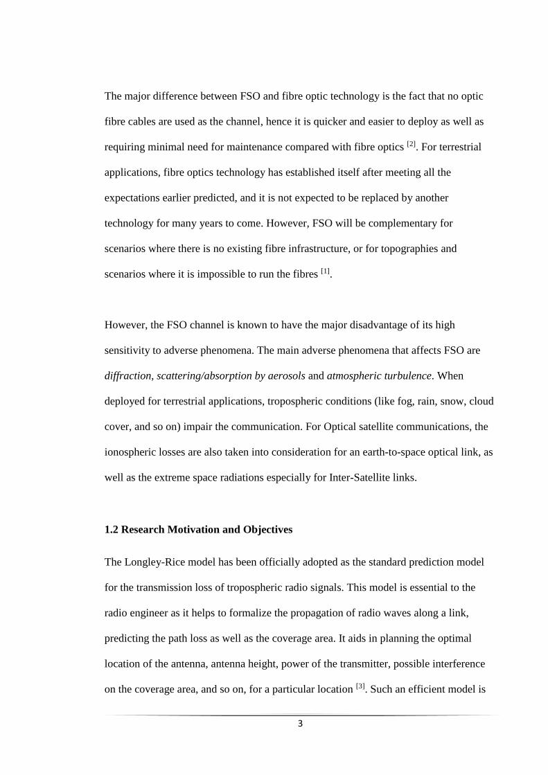
case and this forms part of the researcher’s proposed future work. Figure 1 summarises
the research approach.
5
Fig.1: Research Approach
Literature Review
A detailed review of past works done in this area was completed, going over some basic
concepts on wave propagation through the atmosphere, channel impairments, and
previous optical beam propagation models. These added to the library of facts needed to
develop a robust model. Before commencing the simulation, some system models
needed to be developed mathematically based on some of the reviewed existing theory.
Software Analysis
The MATLAB has proven to be an invaluable tool for such simulations as this, other
software options are Mathematica, Labview, and Light-pipes. The desired software
should be able to model up to six different atmospheric conditions and the
corresponding effect on the received signal. MATLAB was eventually the chosen
software as it is easier to adapt to suit the research.
Model Development
Engineering modelling is becoming more popular due to the high cost of implementing
experiments. This stage entails implementing on software, the system models earlier
developed from the literature. The two different beams where modelled first, then the
beam propagation was modelled, also including the effect of atmospheric turbulence.

6
The robustness of MATLAB also aided an effective presentation of the results based on
different performance measures.
Comparative Evaluation:
The developed model was evaluated with the earlier defined system models, established
hypotheses and compared with other available results obtained from the literature. This
was necessary to ensure the model is performing as expected. If not, the whole process
is repeated from the Software Analysis as seen from the Fig. 1.
1.4 Related Past Researches
In the last century, the effect of turbulence in Optical communication has received a lot
of attention from optical physicists and optical communications engineers. Quite a lot of
work has been done to characterise the propagation of Gaussian beams, which is the
common beam profile from most lasers. However due to diffraction, the Gaussian beam
suffers from beam spreading resulting in severe loss of its initial energy and poor signal
to noise ratio at the receiver. To address this, Durnin [9] proposed a cylindrically-
symmetric non-diffracting beam called the Bessel beam, with a central core surrounded
by a set of same-energy-level concentric rings. Some authors have shown that the
central core of a Bessel beam is resistant to diffractive spreading compared to that of a
Gaussian beam with similar beam radius [10,11].
The Bessel beam can be decomposed into an infinite set of plane wavefronts at different
azimuths, but at a fixed inclination towards the direction of travel. When propagating,
the wavefronts travel inwardly adding up to the energy of the central core [9,12,13]. This
7
inward diffraction is what helps its on –axis intensity to remain constant as it propagates.
Another effect of the inward diffraction is an attribute called self- healing: the beam is
capable of recovering back its profile down the path after being scattered by an
obstruction. These properties make Bessel beams very promising for various
applications like the FSO Communications as well as observatory astronomy.
This research will investigate the possible improvement to FSO by modelling the
propagation of this Bessel beam through free space, and comparing it with the Gaussian
beam. The additional effect of atmospheric turbulence on the propagating beam will
also be considered. Modelling the turbulence in the atmospheric channel is a very
critical consideration in designing an FSO system. Nelson et al [12] investigated the
propagation of these two beams (Gaussian and Bessel beams) over a short ground-to-
ground range of 6.4km, with a fixed strength of turbulence Cn2. In this research, we will
not only look at the ground-to-ground scenario, but will also investigate the more
difficult beams propagation from ground to space. The ground-to-space model we
propose in this work is a modification to the Hufnagel-Andrews-Philips model [14],
considering Cn2 to be larger in the lower atmosphere but gradually weakening with
altitude. From our ground-to-space model, we define a maximum altitude of 22 km
above which the effect of atmospheric turbulence is considered negligible. Beyond this
altitude and up to 100 km height, the beams propagate in vacuo.
1.5 Research Achievements
We have been able to bring some contributions to the vast research going on globally
with the aim of better characterising the medium for Free-Space Optical
8
communications. As mentioned earlier, we proposed our model for Cn2 with respect to
altitude, leading to a definition of a maximum height of 22 km above which turbulence
effect will be negligible.
We have defined some ground-to-space propagation target altitudes and the minimum
beam radius (for both Gaussian and Bessel beams) required to ensure not more than a
half of the initial beam energy is lost. These definitions are based on the known fact that
the longer the distance of the FSO communication, the bigger the required size of the
aperture of the transmitter and receiver to minimise power losses.
We modelled the propagation of the two beams and observed their performances with
and without the presence of atmospheric turbulence. Not only did we model the ground-
to-ground and ground-to-space turbulence scenarios, we also modelled the deep space
scenario were the beams are propagated beyond the 22 km turbulence limit. We
compared the performance of the two beams based on some performance measures:
Beam wander, normalised captured power and RMS intensity error of the propagated
beam compared to the unaberrated beam.
1.6 Dissertation Outline
The rest of this dissertation will first discuss theoretical concepts that are central to the
work, before going ahead to discuss the simulations and results. Chapter 2 will give an
overview of the two kinds of beams that will be considered in this research: the
Gaussian beam and the Bessel beam. A detailed review is carried out for both beams
9
including the Beam profiles and Intensity distributions, energy contained in the beams
as well as a summarised comparison of the beams with each other.
The theory behind the propagation of the beams through atmospheric turbulence is
covered in Chapter 3. This chapter is divided into two sections. The first section is an
Overview of Fourier Optics, covering Maxwell’s equations, Wave equation, Fourier
transform, Scalar Diffraction theory and Sampling theory. The second section is a
review of Atmospheric turbulence, covering its effects on Beam propagation, Phase
screens and Split-step propagation.
The simulations part of this report commences in Chapter 4 where the two beam, to be
propagated, are modelled first. This chapter also covers the derivation of some system
models of power contained in the beams and Atmospheric turbulence, before going
ahead to model it.
Chapter 5 shows the modelling of the propagation of the two beams for a range of 2 km.
We first propagate the beams without atmospheric turbulence to analyse the effect of
diffraction (without turbulence) on the beams. Then we propagate the beams through a
constant turbulence in horizontal 2 km path and finally through gradually-weakening
turbulence in a vertically-upwards 2 km path. The performance of the two beams is
analysed and compared to each other based on some defined performance measures.
The main aim of this chapter is to compare the performance of the beams in a horizontal
path to that of a vertically-upwards path.
10
Chapter 6 provides another perspective to the propagation of the two beams, this time
from ground to a much longer range of 22 km altitude, which will be defined as
turbulence limit. Afterwards, the beams are propagated beyond this turbulence limit
height into deep space. The beam performance is also analysed. The Conclusion and
Recommendations, including proposed Future works are provided in Chapter 7.
Appendix A contains some of the MATLAB functions used for the simulations and
Appendix B shows some of the simulation errors as a result of undersampling and not
adhering to the sampling conditions.

11
CHAPTER 2
12
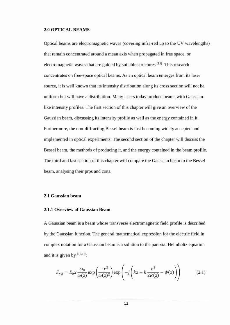
2.0 OPTICAL BEAMS
Optical beams are electromagnetic waves (covering infra-red up to the UV wavelengths)
that remain concentrated around a mean axis when propagated in free space, or
electromagnetic waves that are guided by suitable structures [15]. This research
concentrates on free-space optical beams. As an optical beam emerges from its laser
source, it is well known that its intensity distribution along its cross section will not be
uniform but will have a distribution. Many lasers today produce beams with Gaussian-
like intensity profiles. The first section of this chapter will give an overview of the
Gaussian beam, discussing its intensity profile as well as the energy contained in it.
Furthermore, the non-diffracting Bessel beam is fast becoming widely accepted and
implemented in optical experiments. The second section of the chapter will discuss the
Bessel beam, the methods of producing it, and the energy contained in the beam profile.
The third and last section of this chapter will compare the Gaussian beam to the Bessel
beam, analysing their pros and cons.
2.1 Gaussian beam
2.1.1 Overview of Gaussian Beam
A Gaussian beam is a beam whose transverse electromagnetic field profile is described
by the Gaussian function. The general mathematical expression for the electric field in
complex notation for a Gaussian beam is a solution to the paraxial Helmholtz equation
and it is given by [16,17]:
𝐸𝑟,𝑧 = 𝐸0𝑥𝜔0
𝜔(𝑧)exp (
−𝑟2
𝜔(𝑧)2) exp (−𝑗 (𝑘𝑧 + 𝑘
𝑟2
2𝑅(𝑧)− 𝜓(𝑧))) (2.1)

13
where:
k=wave number for 1 wavelength.
j=√−1, an imaginary unit.
r=radial distance from the centre of the beam.
𝜔0= the beam waist radius.
𝜔(𝑧)=the beam spotsize;
z= the axial distance from the beam source (beam waist).
𝜓(𝑧)= an extra phase term called the Gouy phase shift at point z.
𝐸0= initial electric field, at r = 0 and z = 0.
𝑅(𝑧)= radius of the wavefront of the beam at point z.
These parameters are defined further in the next few pages.
Figure 2.1: Geometry of a Gaussian beam. [Adapted from reference 18]
14
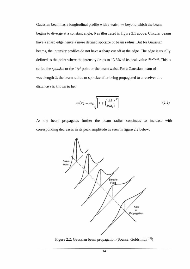
Gaussian beam has a longitudinal profile with a waist, w0 beyond which the beam
begins to diverge at a constant angle, θ as illustrated in figure 2.1 above. Circular beams
have a sharp edge hence a more defined spotsize or beam radius. But for Gaussian
beams, the intensity profiles do not have a sharp cut off at the edge. The edge is usually
defined as the point where the intensity drops to 13.5% of its peak value [19,20,21]. This is
called the spotsize or the 1/e2 point or the beam waist. For a Gaussian beam of
wavelength 𝜆, the beam radius or spotsize after being propagated to a receiver at a
distance z is known to be:
𝜔(𝑧) = 𝜔0√[1 + (𝑧𝜆
𝜋𝜔0)
2
] (2.2)
As the beam propagates further the beam radius continues to increase with
corresponding decreases in its peak amplitude as seen in figure 2.2 below:
Figure 2.2: Gaussian beam propagation (Source: Goldsmith [17])

15
At some point down the propagation path, the spotsize 𝜔(𝑧) of the beam becomes √2
larger than its initial value 𝜔0. This point is called the Rayleigh range 𝑧𝑅 and is given
by:
𝑧𝑅 =𝜋𝜔0
2
𝜆 (2.3)
The on-axis intensity at the Rayleigh range (z=𝑧𝑅) is half of its initial value (at z = 0).
The expression for the spotsize in equation 2.2 above can be re-written in terms of the
Rayleigh range as:
𝜔(𝑧) = 𝜔0√1 + (𝑧𝑧𝑅⁄ )
2
(2.4)
The angle of divergence of the beam θ (in radians) from the waist, as illustrated in
figure 2.1 above, is defined as:
𝜃 ≅𝜆
𝜋𝜔02 (2.5)
This shows that the Gaussian beam with a smaller beam waist radius will diverge more
than one with a larger waist radius, as it propagates. To minimize divergence in the far
field, a laser with large waist radius (aperture) must be ensured. The radius of curvature
of the beam wavefront evolves as the beam propagates on and it is given by equation
2.6. Its initial value is zero at the beam waist position and approaches zero at + and –
infinity [16,17]:
𝑅(𝑧) = 𝑧 [1 + (𝑧𝑅
𝑧)
2
] (2.6)
Furthermore, the Gouy phase shift at z defined earlier as the additional phase term
beyond the phase that can be accounted for by the phase velocity, is given by:
16
𝜓(𝑧) = tan−1 (𝑧
𝑧𝑅) (2.7)
The actual electric field at a particular point is given by the real part of the equation 4.1
above and it is can be expressed as:
𝐸𝑟 = 𝐸0 exp (−𝑟2
𝜔02
) (2.8)
The Fourier transform of a Gaussian beam is also a Gaussian distribution at every point
along the propagation path. The time –averaged Intensity distribution, which is a
Gaussian as well, is given by [16,22]:
𝐼𝑟,𝑧 = 𝐼0 (𝜔0
𝜔(𝑧))
2
exp (−2𝑟2
𝜔(𝑧)2) (2.9)
where 𝐼0 is the on –axis intensity at the beam waist given by 𝐼0 =𝐸0
2
2𝜂⁄ and 𝜂 is the
characteristic impedance of the medium of propagation (𝜂 = 377Ω in free space).
Most real-life lasers produce beams which are only an approximation of the Gaussian
profiles. The degree of variation from the theoretical Gaussian profile is defined by a
quality factor called the M-squared factor, M2. The M-squared is the ratio of the Beam
Parameter Product (BPP) of the real life beam to that of an ideal beam. The BPP, on
the other hand, is a term quality used to describe the product of the beam divergence
angle 𝜃 with the beam waist radius 𝜔0 [23,24].
𝑀2 =𝐵𝑃𝑃𝑟𝑒𝑎𝑙
𝐵𝑃𝑃𝑖𝑑𝑒𝑎𝑙=
(𝜔0𝜃)𝑟𝑒𝑎𝑙
(𝜔0𝜃)𝑖𝑑𝑒𝑎𝑙 (2.10)
For a theoretical Gaussian beam M2=1 but for a real-life one, M2 is greater than 1.
17
2.1.2 Power contained in the Gaussian beam
As the beam propagates down the path, it diverges resulting in losses in the eventual
beam power that reaches the receiver aperture. For a beam with initial total power P0,
the power contained within an aperture of radius, r is [17]:
𝑃𝑟,𝑧 = 𝑃0 [1 − exp (−2𝑟2
𝜔(𝑧)2⁄ )] (2.11)
where 𝑃0 = 𝜋𝐼0𝜔02 2⁄ is the initial beam power at a beam radius 𝜔0. From equation 2.11,
if the radius if the aperture r is equal to the spot size of the arriving beam (r = 𝜔(𝑧)),
then:
𝑃𝑟,𝑧
𝑃0= 1 − exp(−2) ≈ 0.865 (2.12a)
The equation 2.12 implies that for r =𝜔(𝑧), about 86.5% of the beam’s initial power is able
to pass through the aperture. Likewise, for aperture radius r = 1.07𝜔(𝑧), 90% of the beam’s
initial power is able to pass through the aperture. 95% of the initial power flows through an
aperture radius r = 1.224𝜔(𝑧) and 99% through an aperture r = 1.52𝜔(𝑧)[16].
The intensity of the Gaussian beam can be related to the total initial power of the beam
as:
𝐼𝑟,𝑧 =2𝑃0
𝜋𝜔2(𝑧) (2.12b)
18
2.1.3 Peak intensity of a Gaussian Beam
If the limit of the power contained in the aperture in equation 2.11 above is taken, and
dividing it by the area of the aperture which is circular and gradually shrinking with
distance, then that gives the peak intensity at an on-axis (r = 0) position z away from the
beam waist [16, 20,22]:
𝐼0,𝑧 = lim𝑟→0
𝑃0 [1 − exp(2𝑟2
𝜔(𝑧)2⁄ )]
𝜋𝑟2
(2.13)
The above expression in equation 2.13 shows that the on-axis intensity will be high for
a small aperture area of the beam. When the limit is computed using L’Hopital’s rule,
the peak intensity is then given by:
𝐼0,𝑧 =2𝑃0
𝜋𝜔(𝑧)2 (2.14)
2.1.4 Complex Beam Parameter of Gaussian Beam
In order to help simplify mathematical analyses of Gaussian beam propagation, for
example using ray transfer matrices to analyse the optical resonator cavities [25], the
Gaussian beam is expressed in terms of a complex beam parameter q(z). This complex
beam parameter was introduced in the early days of laser theory and has become a
widely acceptable notation in the field. It is expressed in terms of propagation distance z
and Rayleigh range 𝑧𝑅 as [16,24]:
𝑞(𝑧) = 𝑧 + 𝑖𝑧𝑅
(2.15)
19
The equations 2.16 and 2.17 below show that the reciprocal of q (z) comprises the
radius of curvature of the beam in the real part and the relative on-axis intensity in the
imaginary part.
1
𝑞(𝑧)=
1
𝑧 + 𝑖𝑧𝑅=
𝑧
𝑧2 + 𝑧𝑅2 − 𝑖
𝑧𝑅
𝑧2 + 𝑧𝑅2
(2.16)
1
𝑞(𝑧)=
1
𝑅(𝑧)− 𝑖
𝜆
𝜋𝜔2(𝑧) (2.17)
When the equations for Gaussian beam electric fields defined earlier is expressed in this
form, it is largely simplified. Hence the circular beam field is given by (details of
derivation can be found in reference 16):
𝐸𝑟,𝑧 =1
𝑞(𝑧)exp(−𝑖𝑘
𝑟2
2𝑞(𝑧)) (2.18)
2.1.5 Higher Order Gaussian Modes
In the earlier sections, only one solution of the paraxial wave equation has been
considered and this was a Gaussian beam whose width changes as it propagates down
its axis. This is certainly the most widely-used solution. However, there are other higher
order solutions to the wave equations with beam spot size and radius of curvature of
similar attributes as those of the fundamental mode in previous sections, but their phase
shifts are different. The higher order modes form a complete and orthogonal set of
functions called the modes of propagation [17,20]. All arbitrary distribution of
monochromatic light can be expanded in terms of these two modes which are:
20
(a) Modes in the Cartesian coordinates, also called Hermite-Gaussian mode:
This mode is used to approximate beam profiles from lasers that are asymmetric
in the rectangular coordinate.
(b) Modes in the Cylindrical coordinates, also called Laguerre-Gaussian mode:
This mode is suitable to be used to solve beam profiles that are circularly
symmetrical and are written using the Laguerre polynomials [26].
Further details about these two modes can be found in reference 17.
More recently, some more higher-order modes have been discussed. They are the modes
in elliptical coordinates called the Ince-Gaussian mode [27] and another cylindrical
coordinate mode called the Hypergeometric-Gaussian modes [28].

21
2.2 Bessel beam
2.2.1 Overview of Bessel Beam
Bessel beam is also a solution to the Helmholtz equation in circular cylindrical
coordinates. It is an electromagnetic field whose amplitude is described by the Bessel
function of the first kind. It was introduced by Durnin [9] in 1987, who derived the beam
profile from the wave equation as follows:
(∇2 −1
𝑐2
𝜕2
𝜕𝑡2) 𝐸𝒓,𝑡 = 0 (2.19)
The exact solution of the wave equation in equation 2.19 above for scalar fields
propagating into the region z ≥ 0 is given as:
𝐸𝑥,𝑦,𝑧≥0,𝑡 = exp [𝑖(𝑘𝑧𝑧 − 𝜔𝑡)] ∫ 𝐴(𝜙) exp[𝑖𝑘𝑟(𝑥𝑐𝑜𝑠𝜙 + 𝑦𝑠𝑖𝑛𝜙)] 𝑑𝜙2𝜋
0
(2.20)
where 𝐴(𝜙) is an arbitrary complex function of 𝜙 and 𝑘𝑟2 + 𝑘𝑧
2 = 𝑘 = (𝜔 𝑐⁄ )2 =
wave number. The equation 2.20 above represents a class of non-diffracting fields when
𝑘𝑧 is real, in the sense that the time-averaged intensity distribution at z = 0 is exactly
reproduced for all z > 0, in every plane that is transverse to the z axis:
𝐼𝑥,𝑦,𝑧≥0 = 12⁄ |𝐸𝒓,𝑡|
2= 𝐼𝑥,𝑦,𝑧=0
(2.21)
When 𝐴(𝜙) in equation 2.20 is not dependent on 𝜙, a non-diffracting beam of axial
symmetry is obtained whose amplitude is proportional to:
𝐸𝒓,𝑡 = exp [𝑖(𝑘𝑧𝑧 − 𝜔𝑡)] ∫ exp [𝑖𝑘𝑟(𝑥𝑐𝑜𝑠𝜙 + 𝑦𝑠𝑖𝑛𝜙)]𝑑𝜙
2𝜋
2𝜋
0
(2.22)
22
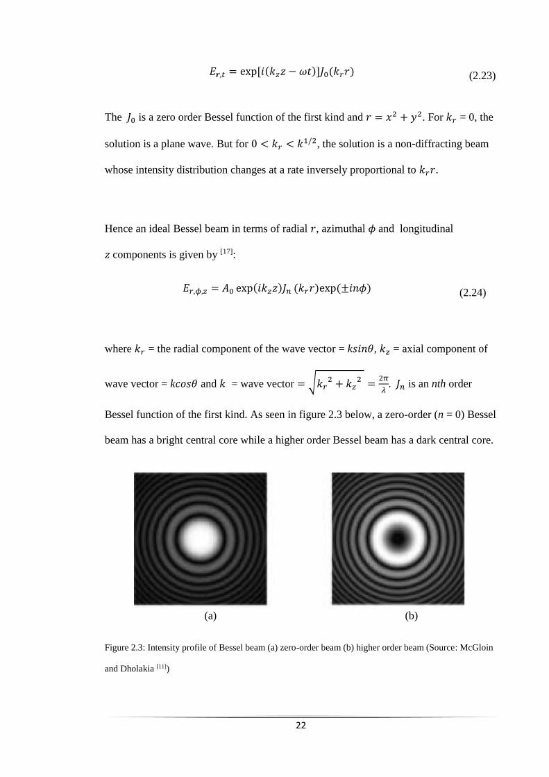
𝐸𝒓,𝑡 = exp [𝑖(𝑘𝑧𝑧 − 𝜔𝑡)]𝐽0(𝑘𝑟𝑟) (2.23)
The 𝐽0 is a zero order Bessel function of the first kind and 𝑟 = 𝑥2 + 𝑦2. For 𝑘𝑟 = 0, the
solution is a plane wave. But for 0 < 𝑘𝑟 < 𝑘1/2, the solution is a non-diffracting beam
whose intensity distribution changes at a rate inversely proportional to 𝑘𝑟𝑟.
Hence an ideal Bessel beam in terms of radial 𝑟, azimuthal 𝜙 and longitudinal
𝑧 components is given by [17]:
𝐸𝑟,𝜙,𝑧 = 𝐴0 exp(𝑖𝑘𝑧𝑧)𝐽𝑛 (𝑘𝑟𝑟)exp (±𝑖𝑛𝜙) (2.24)
where 𝑘𝑟 = the radial component of the wave vector = k𝑠𝑖𝑛𝜃, 𝑘𝑧 = axial component of
wave vector = k𝑐𝑜𝑠𝜃 and 𝑘 = wave vector = √𝑘𝑟2 + 𝑘𝑧
2 =2𝜋
𝜆. 𝐽𝑛 is an nth order
Bessel function of the first kind. As seen in figure 2.3 below, a zero-order (n = 0) Bessel
beam has a bright central core while a higher order Bessel beam has a dark central core.
(a) (b)
Figure 2.3: Intensity profile of Bessel beam (a) zero-order beam (b) higher order beam (Source: McGloin
and Dholakia [11])

23
The infinite Bessel beam in equation 2.24 above is only ideal and has to be truncated
into an aperture of radius Bw, in practise. This aperture results in the Bessel beam only
being non-diffracting over a finite distance, Zmax. This can be visualised by considering
a set of plane waves propagating through a cone resulting in some phase shift as shown
in the figure 2.4 below:
Figure 2.4: Bessel beam decomposed into plane waves
Zmax is the shaded portion between point A and X in the figure 2.4 above and it is given
by the expression below:
𝑍𝑚𝑎𝑥 =𝐵𝑤
𝑡𝑎𝑛𝜃=
𝐵𝑤𝑘
𝑘𝑟 (2.25)
Here, 𝜃 is the cone angle or the deviation angle of the beam’s plane wavefront from the
axis of travel defined as follows:
𝜃 = tan−1𝑘𝑟
𝑘𝑧 (2.26)
𝜃 = (𝑛 − 1)𝛼 (2.27)
24
where n is the refractive index of the axicon material and 𝛼 is the base angle of the cone.
Equation 2.25 above shows that to propagate a Bessel beam to a long distance, either
𝐵𝑤 has to be large, making the telescope inconveniently large, or 𝑘𝑟 must be made
small. By limiting 𝑘𝑟 such that the aperture function radius is equal to the Bessel
function’s first root defined as [11]:
𝐵𝑤 =2.405
𝑘𝑟 (2.28)
we can determine the maximum possible propagation distance:
𝑍𝑚𝑎𝑥 =𝐵𝑤
2𝑘
2.405 (2.29)
This allows us to directly equate the maximum distance the beam can propagate with
the radius of the transmitter telescope.
Bessel beam possesses a profile that is cylindrically symmetrical: a central core
surrounded by a set of nearly-same-energy-level concentric rings. It has been validated
that the central core of a Bessel beam is remarkably resistant to diffractive spreading
compared to a Gaussian beam with spot size equal to the width of the central core of the
Bessel beam [9,10].When propagated, the outer rings of Bessel beams diffract inwardly
adding up to the energy of the central core [9,12,13]. This inward diffraction is what helps
its on –axis intensity to remain constant as it propagates.
25
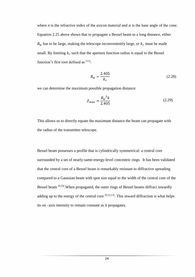
Figure 2.5: Bessel beam self-healing (Source: McGloin and Dholakia [11])
Another effect of the inward diffraction is an attribute called self- healing: the beam is
capable of recovering back its profile down the path after being scattered by an
obstruction. If an object is placed at the centre of the propagating beam, the set of plane
waves that create the beam are able to move beyond the obstruction leaving a shadow
into the beam. But eventually the beam intensity profile is recreated beyond the
obstruction as shown in figure 2.5. This is due to the conical wavefront of the beam [9].
Geometrically, the minimum distance after which the beam is able to regain its profile is
given by:
𝑧𝑠𝑒𝑙𝑓ℎ𝑒𝑎𝑙𝑖𝑛𝑔 ≈𝑚𝑘
2𝑘𝑧 (2.30)
where m is the width of the obstruction object measured from the centre of the beam.
26
For a Bessel beam to have its diffraction free attributes, it has to be ideal, with infinite
radius and this is not physically realisable. Nevertheless in reality, the apertured Bessel
beam can be designed such that it still maintains its desirable non-diffracting attributes
over extended distances.
These properties make Bessel beams very promising for various application like the
Free Space Optical Communications as well as observatory astronomy. Despite its
diffraction-free attribute demonstrated in its longer depth of field, one major downside
of the Bessel beam is known to be that each ring carries about the same energy level as
the central core which means that the more the number of rings, the less the amount of
energy carried by the central core. However, Durnin and his colleagues [29] pointed out
that although this fact might seem obvious, it is not necessarily correct. Gaussian beam
on the other hand, concentrates the energy but has less depth of field.
2.2.2 Energy contained in Bessel Beam and Power Transferred
An ideal Bessel beam is infinite in radius and consequently infinite in its diffraction-free
depth, Zmax as well as energy contained. But as earlier mentioned, practical Bessel
beams are apertured with a finite Zmax and carry a finite amount of energy. Basically, the
power contained in the Bessel beam apertured to radius Bw can be obtained by
integrating the Bessel beam field in equation 2.24 as:
𝑃𝐵𝑤= 𝐴0
2 ∫ ∫ 𝐽02 (𝑟𝑘𝑟)𝑟𝑑𝑟𝑑𝜙
𝐵𝑤
0
2𝜋
0
(2.31)
𝑃𝐵𝑤= 𝐴0
2𝐵𝑤2 𝜋(𝐽0(𝑘𝑟𝐵𝑤)2 + 𝐽1(𝑘𝑟𝐵𝑤)2)
(2.32)
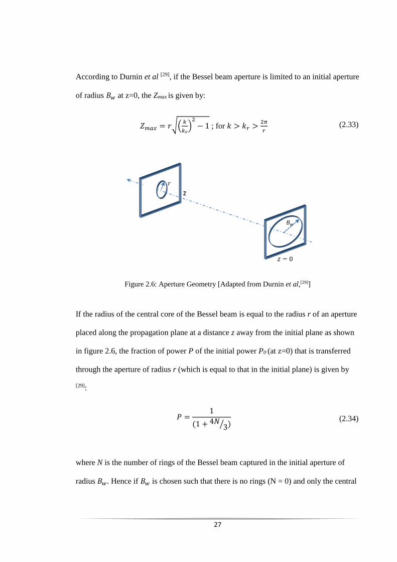
27
According to Durnin et al [29], if the Bessel beam aperture is limited to an initial aperture
of radius 𝐵𝑤 at z=0, the Zmax is given by:
𝑍𝑚𝑎𝑥 = 𝑟√(𝑘
𝑘𝑟)
2
− 1 ; for 𝑘 > 𝑘𝑟 >2𝜋
𝑟 (2.33)
Figure 2.6: Aperture Geometry [Adapted from Durnin et al,[29]]
If the radius of the central core of the Bessel beam is equal to the radius r of an aperture
placed along the propagation plane at a distance z away from the initial plane as shown
in figure 2.6, the fraction of power P of the initial power P0 (at z=0) that is transferred
through the aperture of radius r (which is equal to that in the initial plane) is given by
[29]:
𝑃 =1
(1 + 4𝑁3⁄ )
(2.34)
where N is the number of rings of the Bessel beam captured in the initial aperture of
radius 𝐵𝑤. Hence if 𝐵𝑤 is chosen such that there is no rings (N = 0) and only the central
28
spot fills up the initial aperture, then P in equation 2.34 will be equal to 1 meaning no
power loss. If the Zmax in equation 2.33 is expressed in terms of r, it will be expressed as:
𝑍𝑚𝑎𝑥 ≈𝜋𝐵𝑤𝑟
𝜆⁄ (2.35)
From equation 2.35 above, Bw is derived as:
𝐵𝑤 = 𝜆𝑧𝜋𝑟⁄ (2.36)
Hence, the fraction of power P of the initial power transferred through aperture r is
given as:
𝑃 =𝑟
𝐵𝑤=
𝜋𝑟2
𝜆𝑧 (2.37)
where the total initial power P0 is defined as:
𝑃0 = (𝑐
2𝜋) 𝐴0
2𝐵𝑤
𝑘𝑟 (2.38)
and the c is the speed of light and A0 is the Bessel beam amplitude defined as:
𝐴02 = (
4𝜋
𝑐) (
𝑃0
𝐵𝑤𝑟) (2.39)
2.2.3 Bessel beam Production
Bessel beams are produced mainly by two methods namely [30]:
Using refractive axicon lenses called Durnin rings, and
Using diffractive elements called holographic plates.

29
2.2.3.1 Axicon or Durnin Ring Method
The most common method is using the axicon – a conical lens. Axicons convert the
incoming collimated light into waves propagating through its conical surface which are
approximations of Bessel beams [31,32].
Figure 2.7: Bessel beam generation using an axicon [33]
Bessel beam produced using the axicon method only exist at the near field as seen in the
figure 2.7 above, while an annular ring is formed at the far field. Since the Bessel beam
has an annular ring in its far field, they can be generated, as done by Durnin et al [34,35],
by combining an annular slit with a Fourier transforming lens [33]. The set up Durnin et
al used here was a coherent plane wave illuminating the thin annular slit placed along
the focal plane of a positive lens. They demonstrated satisfactory agreement with the
initial prediction and their experimentally measured transverse and longitudinal
intensity distributions. If the aperture of the lens was infinite, the conical Bessel
wavefront after the lens would have been independent of the distance of propagation.
However since the aperture of the lens will have to be truncated in practice, the Bessel
beam wavefront will exist for a limited distance, Zmax.
30
The Durnin ring method has the advantage of being compatible with microfabrication
technology as the rings can easily be fabricated in mass production using conventional
lithography techniques. This method is also simple and easy to align. However, this
method has a disadvantage of having a small amount of energy passing through the ring,
and hence transported by the resulting beam [31]. If one attempts to increase the size of
the ring in order to allow more power, it will reduce the beam quality. The axicon
method, on the other hand is more efficient than the ring method as it utilises the whole
or most of the incident Gaussian beam.
2.2.3.2 Holographic Plates Method
The alternative experimental set up for generating an approximate Bessel beam is using
a holographic optical element (HOE) [36]. Here, the incident plane wave is directly
modulated in amplitude or in phase by a computer – generated hologram (CGH) often
implemented using a Spatial light modulator (SLM) [37]. A good number of authors have
implemented the phase modulation holographs, which encode the CGH with the phase
profile [38,39,40,41]:
𝑇𝜌,𝜃 = exp(𝑖𝑛𝜃) exp(−𝑖2𝜋𝑟
𝑘𝑟) (2.40)
The HOE performs the conversion of incident plane wave to a conical wave with the
attributes of a Bessel beam. Again in this method, the HOE aperture is finite and this
implies that the resulting Bessel beam will be limited to the distance Zmax but using this
method, the Zmax is twice that for the first method, which gives the holographic method
an advantage.
31
Furthermore, the holographic method offers up to a 100% power conversion efficiency
from the input flat top beam to resulting approximate Bessel beam. The intensity
distribution of the resulting Bessel beam was satisfactorily similar to the theoretical
Bessel beam. However, it was observed that the peak intensity of the central core varied
with distance, with a maximum towards the end of the useful focal range [42].
Some work has also been done to show that higher order non-diffracting beams can be
experimentally generated using holographic elements [40,43].
2.3 Comparison of Gaussian and Bessel Beams
Some authors have done some work in the past attempting to compare these two beams
[29, 44]. The first basis for comparison is energy focusing and diffraction attributes.
Gaussian beams concentrate the energy but are known to be diffracting the energy as it
propagates. On the other hand, Bessel beams are non-diffracting but do not concentrate
all its energy along the central axis. The central core of the Bessel beam is known to
possess desirable non-diffractive attributes. However, since each of the side lobes has
nearly equal energy with the central core, a Bessel beam with say more than 20 side
rings will have less than 5% of the energy in the central core. This off-axis energy waste
is a major disadvantage for the Bessel beam compared to the Gaussian beam whose
energy is more localized with up to 50% of its energy within the Full Width Half
Maximum (FWHM). This fact is still in debate out there [29].
Another basis of comparison of these two beams will be the definition of their spot sizes
or beam radius. It is generally easier to define the spot size of a beam that has a well-

32
defined and sharp edge. The Gaussian beam intensity profile does not have a sharp edge.
Its spot size is usually defined as the 1/e2 point, which is the point when the intensity
drops to 13.5% of its peak value. The Bessel beam, on the other hand, reaches its first
zero at a well specified value, 𝐽1(3.8) = 0, which is the first root (dark ring) and this a
region of destructive interference. Hence, the spot size of a Bessel beam is the radius of
its central core [19]. Hence generally speaking, the comparison between Bessel and
Gaussian beams is usually between the Bessel beam’s central core and a Gaussian beam
of similar spot size.
With respect to beam divergence, the Gaussian beam spreads by a factor of √2 at the
Rayleigh range position while the central core of the Bessel beam remains free from
spreading within its Zmax which is comparable to the Rayleigh range. If both Gaussian
and Bessel beams have the same FWHM at the initial plane (z = 0), Durnin et al [29]
defined a relationship in terms of the distance at which their peak intensity drops to 50%
of its initial value, 𝑍0.5𝐼𝑛𝑡𝑒𝑛𝑠𝑖𝑡𝑦. The Bessel beam’s half-intensity distance is given as:
𝐵𝑒𝑠𝑠𝑒𝑙 𝑍0.5𝐼𝑛𝑡𝑒𝑛𝑠𝑖𝑡𝑦 ≈ 𝐺𝑎𝑢𝑠𝑠𝑖𝑎𝑛 𝑍0.5𝐼𝑛𝑡𝑒𝑛𝑠𝑖𝑡𝑦 × 𝑁 (2.41)
where N is the number of rings of the Bessel beam at the initial plane. It is clear from
equation 2.41 that the more the number of rings N of the Bessel beam, the longer its
non-diffracting distance. In addition, since the total integral power in each ring of the
Bessel beam is roughly equal to that in the central core, a similar relation occurs for the
total power in the beams:
𝐵𝑒𝑠𝑠𝑒𝑙 𝑃𝑡𝑜𝑡𝑎𝑙 ≈ 𝐺𝑎𝑢𝑠𝑠𝑖𝑎𝑛 𝑃𝑡𝑜𝑡𝑎𝑙 × 𝑁 (2.42)
33
2.4 Chapter Summary
This chapter covered the basic theory on the Gaussian and Bessel beams. For the
Gaussian beam, we did a review of the beam profile, power contained in the beam, the
peak intensity, the complex beam parameter and the higher order Gaussian beams. For
the Bessel beam, we covered the beam profile, the energy contained in the beam, the
power transferred in the beam and the two beam production methods: the holographic
plate method and the Durnin ring method. We dedicated a full section to discuss on the
comparison of the attributes of the two beams based on energy focusing and diffractive
attributes, definition of their spot sizes and beam divergence.

34
CHAPTER 3
35
3.0 THE THEORY OF FREE SPACE OPTICAL PROPAGATION THROUGH
ATMOSPHERIC TURBULENCE
In this chapter, the theory behind the propagation of the two optical beams analysed in
chapter two, the Gaussian beam and Bessel beam, is considered. One of the main
techniques used for modelling the propagation of beams from one point to another is
called Fourier Optics. An overview of Fourier optics, starting from the Maxwell’s
equations down to sampling theory, is what comprises the first section of this chapter.
The second section will encapsulate the theory of atmospheric turbulence, its causes, its
effects on the propagated beam and how it can be modelled on the computer.
3.1 Overview of Fourier Optics
Since the advent of the discipline of Fourier Optics in the 1940s, it has become
fundamental in the analysis of imaging, diffraction, holography and even in applications
like wave propagation through random media. It utilises Fourier transforms in the study
of classical optics. In Fourier optics, the optical wave is considered as a superposition of
plane waves that are not traceable to any identifiable source. This section of the chapter
essentially summarises some basics of Fourier Optics starting from derivations of the
fundamental preliminary theories like the Maxwell’s equations, wave equation and
Helmholtz equation which are the building blocks for Fourier optics. This section will
also cover the Fourier transform which is an important tool in Fourier Optics. Next, the
Scalar Diffraction theory will be summarised here, which describes the evolution of an
optical field as it propagates from source to destination. The last sub-section expatiates
on the constraints considered when sampling the real signals onto computer simulations.

36
3.1.1 Maxwell’s Equations
Maxwell’s equation is a set of paraxial differential equations that describes the electric
field and the magnetic field, as well as the relationship between these two fields, electric
charge and currents. Although Maxwell’s equations are only approximations and not
absolutely accurate, their solutions encompass all the diverse set of phenomena in
classical electromagnetism. In Fourier optics, optical fields are seen as solutions to the
Maxwell’s equation, hence the need for it to be summarised here. Jason Schmidt [45] did
a thorough job in deriving these equations and his notation will be followed in this
section.
The interaction of any test charge with any bulk material of non-zero volume current
density J, volume polarisation density P and volume magnetisation density M,
generates a force on the charge. This electrostatic force, as described by Lorentz force
law, is a function of two field vectors; the electric field, E and the magnetic induction, B
[46]:
𝐹𝑒𝑙𝑒𝑐𝑡𝑟𝑜𝑠𝑡𝑎𝑡𝑖𝑐 = 𝑞(𝐄 + 𝑣 × 𝐁) (3.1)
The force is either in same direction or opposite direction to the field, hence the name
push-and-pull force. When these two fields were related to the sources, Maxwell’s
equations were derived experimentally and mathematically. The Maxwell’s equations
describe the Faraday’s law:
∇ × 𝐄 +𝜕𝐁
𝜕𝑡= 0
(3.2)
and the Ampere’s law:
37
∇ × 𝐁 − 𝜖0𝜇0
𝜕𝐄
𝜕𝑡= 𝜇0 (𝐉 +
𝜕𝐏
𝜕𝑡+ ∇ × 𝐌)
(3.3)
where 𝜖0 is the permittivity of free space or electric constant and 𝜇0 is permeability of
free space or magnetic constant. When the Ampere’s law in equation 3.3 is re-expressed
in a more functional form as:
∇ × (𝐁
𝜇0− 𝐌) = 𝐽 +
𝜕
𝜕𝑡(𝜖0𝐄 + 𝐏)
(3.4)
then the definitions for the medium’s response to the applied fields, electric
displacement D and magnetic field H, can be made:
𝐃 = 𝜖0𝐄 + 𝐏
(3.5)
𝐇 =𝐁
𝜇0− 𝐌
(3.6)
Hence, the Maxwell’s equations are now re-expressed as:
∇ × 𝐄 = −𝜕𝐁
𝜕𝑡
(3.7)
∇ × 𝐇 = 𝐉 +𝜕𝐃
𝜕𝑡
(3.8)
Furthermore, after relating equation 3.7 and 3.8 with the conservation of charge and
performing some algebraic manipulation before the source is turned on, Coulomb’s law
(also part of the Maxwell’s equations) is deduced as:
∇. 𝐃 = 𝜌
(3.9)
∇. 𝐁 = 0
(3.10)

38
It is necessary to define a few relations in order to apply Maxwell’s macroscopic
equations, which have an undesirably high number of unknown scalars and vectors.
These relations are called Constitutive relations [47] and they are as follows:
𝐏 = 𝜖0𝜒𝑒𝐄
𝐌 = 𝜒𝑚𝐇
𝐃 = 𝜖𝐄
𝐁 = 𝜇𝐇
(3.11)
where 𝜒𝑒 and 𝜒𝑚 are the electric and magnetic susceptibilities respectively and 𝜖 and 𝜇
are the electric permittivity and magnetic permeability respectively. Substituting the
constitutive relations into equations 3.7 and 3.8 simplifies them to:
∇ × 𝐄 = −𝜇𝜕𝐇
𝜕𝑡
(3.12)
∇ × 𝐇 = 𝐉 + 𝜖𝜕𝐄
𝜕𝑡
(3.13)
Hence, the Maxwell’s equations are equations 3.7, 3.8, 3.9, 3.10, 3.12 and 3.13.
3.1.2 Scalar Wave Equation and Helmholtz Equation
The Maxwell’s equations defined in the immediate previous section can be refined into
uncoupled wave equations, written in closed form without an integral. The wave
equation shows that all waves travel at a single speed, which is the speed of light. The
Helmholtz equation, which also shows up in Quantum mechanics and Thermodynamics,
is a time-independent form of the wave equation often used to reduce the complexity of
the analysis.
39
This sub-section will show how the wave equation and the Helmholtz equation are
derived from the Maxwell’s equations (that is the Ampere law and the Faraday’s law),
based on Goodman [48] and Schmidt’s [45] notations. If a source-free region is assumed
here, no charges nor currents are flowing in the medium. This implies that, 𝜇 = 𝜇0, and
𝜌 = 𝐉 = 0, 𝜖 is a scalar independent of wavelength, position in space and time. From
equations 3.12, taking the curl results in:
∇ × (∇ × 𝐄) = −𝜇0
𝜕
𝜕𝑡(∇ × 𝐇)
(3.14)
and substituting equation 3.13 into the above yields:
∇ × (∇ × 𝐄) = 𝜇0𝜖𝜕2
𝜕𝑡2𝐄
(3.15)
By vector identity to the LHS of equation 3.15, it becomes:
∇(∇. 𝐄) − ∇2𝐄 = 𝜇0𝜖𝜕2
𝜕𝑡2𝐄
(3.16)
Substituting equation 3.9 and 𝐃 = 𝜖𝐄 from equation 3.11 into equation 3.16 now yields:
∇2𝐄 − 𝜇0𝜖𝜕2
𝜕𝑡2𝐄 = 0
(3.17)
where 𝛻2 is the Laplacian operator. Similarly, taking the curl of 3.13, substituting
equation 3.12 into it, applying the vector identity and equivalent substitutions yields a
corresponding equation for magnetic field:
∇2𝐁 − 𝜇0𝜖𝜕2
𝜕𝑡2𝐁 = 0
(3.18)
40
For the purpose of simplification, when the vector field E and B are now replaced a
common term for scalar field in the Cartesian coordinate, it results in the Scalar Wave
Equation given as:
(∇2 − 𝜇0𝜖𝜕2
𝜕𝑡2) 𝑈𝒙,𝒚,𝒛 = 0
(3.19)
The Scalar Wave equation can also be expressed in terms of the speed of light 𝑐 =1
√𝜇0𝜖0
and refractive index 𝑛 = √𝜖𝜖0⁄ below:
(∇2 −𝑛2
𝑐2
𝜕2
𝜕𝑡2) 𝑈𝒙,𝒚,𝒛 = 0
(3.20)
According to Goodman [48], all components of a linear, homogenous, isotropic and
nondispersive dielectric medium behave identically and their behaviour is described by
a single Scalar wave equation. The scalar theory is known to be accurate as long as the
diffracting structures are large compared with the wavelength of the light signal. Optical
signals comprise electric field E and magnetic field B that are time harmonic travelling
waves. Hence substituting exp(−𝑖2𝜋𝑣𝑡) into equation 3.20 yields the Helmholtz
equation:
[∇2 + (2𝜋𝑛𝑣
𝑐)
2
] 𝑈 = 0
(3.21)
In terms of the wave number 𝑘 = 2𝜋 𝜆⁄ and wavelength 𝜆 = 𝑐 𝑣⁄ , the Helmholtz
equation is commonly expressed as:
[∇2 + 𝑘2𝑛2]𝑈 = 0
(3.22)
41
3.1.3 Review of Fourier Analysis
Fourier analysis is a very important tool in Fourier Optics as well as Electrical networks,
useful for the analysis of linear and non-linear phenomena. The fundamental
mathematical concepts of the Fourier theory is well treated by Bracewell [49]. The
following sections will cover the Fourier analysis of functions of two independent
variables, also covered by Goodman [48].
3.1.3.1 Definition of analytical Fourier Transform
The analytical Fourier transform of a 2-dimentional spatial function 𝑔(𝑥, 𝑦) is defined
as:
𝐺(𝑓𝑥, 𝑓𝑦) = ℑ{𝑔(𝑥, 𝑦)} = ∫ ∫ 𝑔(𝑥, 𝑦)𝑒−𝑖2𝜋(𝑓𝑥𝑥+𝑓𝑦𝑦)𝑑𝑥𝑑𝑦
∞
−∞
∞
−∞
(3.23)
where 𝑓𝑥 and 𝑓𝑦 are independent spatial-frequency variables associated with spatial
variables x and y. The analytical reverse, called the inverse Fourier Transform, is given
by:
𝑔(𝑥, 𝑦) = ℑ−1{𝐺(𝑓𝑥 , 𝑓𝑦)} = ∫ ∫ 𝐺(𝑓𝑥, 𝑓𝑦)𝑒𝑖2𝜋(𝑓𝑥𝑥+𝑓𝑦𝑦)𝑑𝑓𝑥𝑑𝑓𝑦
∞
−∞
∞
−∞
(3.24)
The above two definitions of the Fourier transform is only mathematically realisable if
the function 𝑔(𝑥, 𝑦) satisfies the conditions listed below [48, 50]:
i. 𝑔(𝑥, 𝑦) must have only a finite number of discontinuities.
ii. 𝑔(𝑥, 𝑦) must be absolutely integrable over the infinite range of x and y.
iii. 𝑔(𝑥, 𝑦) must have no infinite discontinuities.

42
However, it has been demonstrated that some of the above conditions can be weakened
in some important cases, and proposed an idealised transform approach to be used to
find useful transform representations [48]. In Fourier analysis, the Fourier Transform
defined in equation 3.23 and 3.24 have some basic mathematical properties presented as
the theorems listed below:
I. Linearity theorem
II. Similarity theorem
III. Shift theorem
IV. Rayleigh’s or Parseval’s Theorem
V. Convolution theorem
VI. Autocorrelation Theorem
VII. Fourier integral theorem.
Table 3.1: Fourier Transforms of basic functions
Functions Definition Fourier Transform
Rectangle 𝑟𝑒𝑐𝑡 (𝑥
𝑎)
|𝑎|𝑠𝑖𝑛𝑐(𝑎𝑓𝑥)
Sinc 𝑠𝑖𝑛𝑐 (𝑥
𝑎)
|𝑎|𝑟𝑒𝑐𝑡(𝑎𝑓𝑥)
Triangle Λ (𝑥
𝑎) |𝑎|𝑠𝑖𝑛𝑐2(𝑎𝑓𝑥)
Comb 𝑐𝑜𝑚𝑏 (𝑥
𝑎) |𝑎|𝑐𝑜𝑚𝑏(𝑎𝑓𝑥)
Circle 𝑐𝑖𝑟𝑐 (
√𝑥2 + 𝑦2
𝑎) 𝑎2
𝐽1(2𝜋𝑎√𝑓𝑥2 + 𝑓𝑦
2
𝑎√𝑓𝑥2 + 𝑓𝑦
2
Chirp exp [−𝜋 (
𝑥2
𝑎2+
𝑦2
𝑏2)]
|𝑎𝑏| exp[−𝜋(𝑎2𝑓𝑥2 + 𝑏2𝑓𝑦
2)]
43
Since different basic functions are used to describe various physical or analytical
apertures and structures in optics, then defining the Fourier Transforms of the basic
functions can be useful in finding diffraction solutions. The table 3.1 above presents the
basic functions and their Fourier Transforms, as highlighted by David Voelz [50].
3.1.3.2 Discrete Fourier Transform
For modelling the Fourier optics problem, the analytical continuous Fourier optics
expression in equation 3.23 has to be discretized; this is called the Discrete Fourier
Transform (DFT). The forward and inverse Discrete Fourier Transform, as will be
defined in this section, are not usually directly implemented for simulations, but are
most efficiently presented in the form called the Fast Fourier Transform (FFT). FFT
algorithms are not most efficient when M and N are of a power of 2. The Fourier
Transform in equation 3.23 can be approximated using a Riemann sum, substituting for
the equation
∫ ∫ … 𝑑𝑥𝑑𝑦
∞
−∞
∞
−∞
(3.25)
with
∑ ∑ … ∆𝑥∆𝑦
𝑀2⁄ −1
𝑚=−𝑀2⁄ −1
𝑁2⁄ −1
𝑛=−𝑁2⁄ −1
(3.26)
Although the ∆𝑥∆𝑦 is not included in the DFT definition which operates on discrete
values without details of sample intervals, it is needed for appropriate scaling of a
physical problem. The derivation for the expression for the DFT of 𝑔(𝑥, 𝑦) [now
presented here as 𝑔(𝑚, 𝑛)] is given as[50]:
44
𝐺𝐷𝐹𝑇(𝑝, 𝑞) = ∑ ∑ 𝑔(𝑚, 𝑛) exp [−𝑖2𝜋 (𝑝𝑚
𝑀+
𝑞𝑛
𝑁)]
𝑁2⁄ −1
𝑛=−𝑁2⁄
𝑀2⁄ −1
𝑚=−𝑀2⁄ −1
(3.27)
and the inverse DFT of 𝐺𝐷𝐹𝑇(𝑝, 𝑞) as:
𝑔(𝑚, 𝑛) =1
𝑀𝑁∑ ∑ 𝐺𝐷𝐹𝑇(𝑝, 𝑞) exp [𝑖2𝜋 (
𝑝𝑚
𝑀+
𝑞𝑛
𝑁)]
𝑁2⁄ −1
𝑞=−𝑁2⁄
𝑀2⁄ −1
𝑝=−𝑀2⁄
(3.28)
where the continuous frequency domain samples 𝑓𝑥 and 𝑓𝑦 in the continuous Fourier
transforms are now divided into M and N evenly-spaced coordinate values. The p and q
are integer multiples of the frequency sample intervals are defined as −𝑀2⁄ < 𝑝 <
𝑀2⁄ − 1 and −𝑁
2⁄ < 𝑞 < 𝑁2⁄ − 1, and have the same values as m and n respectively.
One major downside of the FFT is seen in indexing of array data values as well as
arrangement of the coordinates. In square grids, it is convenient to a centre the
coordinate position for the function of interest in the vector, for display purposes. But
the centred vector needs to be shifted first before any FFT operation is carried out.
Another major difference between the Discrete Fourier transform and the analytical
Fourier transform is that the results of the DFT has an attribute called periodic extension,
discussed in detail by Brigham [51].
45
3.1.4 Scalar Diffraction
The Scalar Diffraction theory in Fourier Optics describes the propagation of an optical
signal from one point to another, under an ideal condition where the medium of
propagation is assumed to be linear, homogenous, isotropic, nonmagnetic and
nondispersive. Based on the Scalar diffraction theory, the propagation of
electromagnetic waves through a vacuum is analogous to a linear system where a
convolution of a monochromatic electric field magnitude in the source plane and the
impulse response of the free-space channel will result in the electric field magnitude in
the observation plane [48]. This is why Scalar Diffraction is known as the physical basis
of wave optics. The concept of the linear systems, when combined with Fast Fourier
Transform makes it efficient for computation of wave optics scenarios.
When an optical signal is confined to an aperture, the optical signal is said to be going
through Diffraction. Unlike reflection and refraction which are more obvious in our
everyday life, diffraction is only noticed when the optical wave is laterally confined to
an aperture of dimension on the order of the wavelength of the optical signal [48, 52].
Hence, Sommerfeld [53] defines diffraction as the deviation of light rays from the
rectilinear paths, which cannot be interpreted as refraction nor reflection. The
diffraction effect is a general attribute of a wave that occurs when a portion of a
wavefront encounters an obstruction resulting in alteration of its amplitude or phase
[54,55]. The interference of the sections of the wavefront that propagates beyond the
obstacle causes an energy distribution called the diffraction pattern.
46
3.1.4.1 The Huygens-Fresnel Principle
Christiaan Huygens [56] proposed a principle that every single point on any wavefront
can be considered as a source of secondary spherical wavelets. The shape of the
wavefront, at every instant, is the envelope of the secondary wavelets. The limitation of
this principle is that it ignores the majority of these secondary wavelets and taking into
consideration only the portions that are common to the envelope. This way, it is unable
to account for most of the diffraction process. This limitation was resolved by Fresnel in
1818 [57], who modified the Huygens’s principle mathematically and added the concept
of interference to it. The resulting Huygens-Fresnel principle states that every
unobstructed point of a waveform, at any instant, serves as a source of spherical
secondary wavelets (with the same frequency as that of the primary wave). The
amplitude of the optical field at any point beyond is the superposition of all these
wavelets, considering all their amplitudes and relative phases. A bit later on in 1882,
Gustav Kirchhoff [58] showed that the Huygens-Fresnel principle was a direct
consequence of the differential wave equation. Sommerfeld eventually modified the
Kirchhoff’s theory by making use of the Green’s function, eliminating the assumption
concerning the amplitude of light. The Sommerfeld’s theory is called the Rayleigh-
Sommerfeld diffraction theory. The Rayleigh-Sommerfeld Diffraction solution is an
accurate and a general expression used to predict field at the observation plane.
Based on the Huygens-Fresnel principle, the observation plane U2(𝑥, 𝑦), at a distance z
from the source field U1(𝜉, 𝜂), in rectangular coordinates, can be written as:
𝑈2(𝑥, 𝑦) =𝑧
𝑖𝜆∬ 𝑈1(𝜉, 𝜂)
𝛴=𝑎𝑝𝑒𝑟𝑡𝑢𝑟𝑒
𝛴
exp (𝑖𝑘𝑟12)
𝑟122 𝑑𝜉𝑑𝜂 (3.29)
47
The 𝑟12 = √𝑧2 + (𝑥 − 𝜉)2 + (𝑦 − 𝜂)2 is the separation between a point on the source
plane and another point of the observation plane, k is the wavenumber and 𝜆 is the
wavelength of the optical signal. Some approximations to this general theory have been
derived which have helped reduce diffraction pattern calculations to simple
mathematical manipulations. These approximations are the Fresnel and Fraunhofer
Diffraction approximations [48].
3.1.4.2 Fresnel Diffraction Approximation
By introducing some binomial approximations for the distance variable r12 in the
general the equation 3.29 above, explained in details by Voelz [52], the Fresnel
approximation is derived as:
𝑈2(𝑥, 𝑦) =𝑒𝑖𝑘𝑧
𝑖𝜆𝑧∬ 𝑈1 (휀, 𝜂)𝑒𝑥𝑝 {𝑖
𝑘
2𝑧[(𝑥 − 휀)2 + (𝑦 − 𝜂)2]} 𝑑휀𝑑𝜂 (3.30)
Equation 3.30 can be expressed as a convolution integral expressed below:
𝑈2(𝑥, 𝑦) = ∬ 𝑈1(휀, 𝜂)ℎ(𝑥 − 휀, 𝑦 − 𝜂)𝑑휀𝑑𝜂 (3.31)
When the Fourier convolution theorem is applied to equation 3.31 above, where both
source and observation planes are parallel and assumed to have the same variables x and
y, the following expression is obtained:
𝑈2(𝑥, 𝑦) = ℑ-1{ℑ{𝑈1(𝑥, 𝑦)}ℑ{h(x,y)}}
(3.32)
48
with its equivalent equation given as:
𝑈2(𝑥, 𝑦) = ℑ -1{ ℑ {𝑈1(𝑥, 𝑦)}H(𝑓𝑋 , 𝑓𝑌)}
(3.33)
Typically, Equations 3.32 and 3.33 above are both similar Fresnel (near field)
diffraction expressions but are liable to produce different results due to some sampling
criteria discussed in detail in section 3.1.5.3. Here, H and h are the Rayleigh-Somerfield
Transfer Function (TF) and Impulse Response (IR) function respectively, given by:
ℎ(𝑥, 𝑦) =𝑒𝑗𝑘𝑧
𝑗𝜆𝑧𝑒𝑥𝑝 [
𝑗𝑘
2𝑧(𝑥2 + 𝑦2)]
(3.34)
𝐻(𝑓𝑋 , 𝑓𝑌) = 𝑒𝑗𝑘𝑧𝑒𝑥𝑝[−𝑗𝜆𝑧𝜋(𝑓𝑋2 + 𝑓𝑌
2)]
(3.35)
Fresnel propagators are modelled by implementing either equations 3.34 or 3.35
depending which one suits the regime under consideration.
The two different forms of Fresnel approximation Integral expression in 3.32 and 3.33
are presented differently to aid numerical evaluations. Jason Schmidt [59] went deeper to
analyse these two forms and calls them the Fresnel Integral and the Angular Spectrum
forms respectively:
3.1.4.2.1 Fresnel Integral Form or Fresnel Transfer Function
The first method is obtained from the equation 3.30 by expanding the squared terms in
the exponential and factoring out the integrals, resulting in the expression:
49
𝑈2(𝑥, 𝑦) =𝑒𝑖𝑘𝑧
𝑖𝜆𝑧𝑒𝑖
𝑘2𝑧
(𝑥2+𝑦2) ∬ [𝑈1(𝜉, 𝜂)𝑒𝑖𝑘
2𝑧(𝜉2+𝜂2)] 𝑒−𝑖
2𝜋𝜆𝑧
(𝑥𝜉+𝑦𝜂)𝑑𝜉𝑑𝜂 (3.36)
This approach can either be a one-step Fourier Transform which is more straightforward
or a two-step propagation which computes the Fresnel integral twice and adds some
flexibility in the grid spacing. The one-step propagation is more efficient
computationally where the observation plane field is obtained by a single Fourier
Transform step: the source field is multiplied by a quadratic phase factor, Fourier
transformed, converted from a spatial frequency coordinate to spatial coordinate, and
multiplied by another quadratic phase factor.
3.1.4.2.2 Angular Spectrum Form or Fresnel Impulse Response
The second method has to do with treating the Fresnel integral in equation 3.30 as a
convolution of the source field and the free-space amplitude spread function:
𝑈2(𝑥, 𝑦) = 𝑈1(𝜉, 𝜂) ⊗ [𝑒𝑖𝑘𝑧
𝑖𝜆𝑧𝑒𝑖
𝑘2∆𝑧
(𝜉2+𝜂2 )] (3.37)
This method has been treated and applied by some authors in the past [60,61].
3.1.4.3 Fraunhofer Diffraction Approximation
The Fraunhofer approximation of the Rayleigh-Sommerfeld diffraction solution has no
impulse response nor transfer function, hence cannot be written as a convolution
integral. It is commonly called the far field diffraction and Goodman [48] expressed it as:
50
𝑈2(𝑥2, 𝑦2) =𝑒𝑖𝑘𝑧𝑒𝑖
𝑘2𝑧
(𝑥2+𝑦2)
𝑗𝜆𝑧∬ 𝑈1(휀, 𝜂)𝑒𝑥𝑝 [−𝑖
2𝜋
𝜆𝑧(𝑥휀 + 𝑦𝜂)] 𝑑휀 𝑑𝜂 (3.38)
The Fresnel number criterion is generally used to determine when the Fresnel
expression can be applied with minimal loss of accuracy or when the Fraunhofer is
suitable. The Fresnel number is given by:
𝑁𝑓 =𝑤2
𝜆𝑧 (3.39)
If Nf is far less than (<<) 1, then the observation plane is generally regarded to be in the
Fraunhofer region. But if Nf is > 1, then it is in the Fresnel zone. However, if the Nf is
less than or equal to 1, it is commonly acceptable that the observation plane is in the
Fresnel region, hence the Fresnel approximation is applied for useful results. It is
considered in Fraunhofer region when Nf is more that 20 to 30 times less than 1.
3.1.5 Sampling Theory
When modelling the wave optics on the computer, functions are represented with
discrete arrays of sampled values, then transforms are applied to them and processed, as
needed. To represent the functions as accurately as possible, the physical element will
need to be represented with several samples, but at the expense of the execution timing
and computing memory requirements. Hence the aim in practical simulations will
always be to strike a balance between these two factors [48,50]. If the function 𝑔(𝑥, 𝑦) is
sampled in the x and y directions with sample interval ∆𝑥 and ∆𝑦 respectively, the
sampling is described as:
51
𝑔(𝑥, 𝑦) → 𝑔(𝑚∆𝑥, 𝑛∆𝑦) (3.40)
where m and n are integers representing the indices of the samples often defined with
the following values, for a finite sampled space with 𝑀 × 𝑁 number of samples:
−𝑀
2≤ 𝑚 ≤
𝑀
2, −
𝑁
2≤ 𝑛 ≤
𝑁
2 (3.41)
The lengths of the physical area Lx and Ly, in the x and y directions respectively, are
given by:
𝐿𝑥 = 𝑀∆𝑥, 𝐿𝑦 = 𝑁∆𝑦 (3.42)
It is important to define a support span area, Dx × Dy within the physical area, Lx × Ly
where the significant part of the values of the function 𝑔(𝑥, 𝑦) will be contained, to
ensure they fit into the physical area. This entails that
𝐷𝑥 < 𝐿𝑥 and 𝐷𝑦 < 𝐿𝑦. (3.43)
It is a good practise to provide an extra area called the guard area around the area of
interest to help reduce artifacts at the edges of the observation array after propagation
due to the periodic extension properties of the FFT. In this case the array side lengths
𝐷𝑥 < 2𝐿𝑥 and 𝐷𝑦 < 2𝐿𝑦 (3.44)
Furthermore, to ensure that the sample intervals ∆𝑥 and ∆𝑦 are small enough to preserve
the features of the function 𝑔(𝑥, 𝑦), the Shannon-Nyquist sampling theory defines a
requirement for bandlimited functions needed to ensure an exact recovery of a
continuous function from the samples. This sampling criterion requires that the sample
intervals be smaller than a specific value, as defined in equation 3.45 below, in terms of
the spectral bandwidths 𝐵𝑥 and 𝐵𝑦 in the x and y directions respectively [48]:
52
∆𝑥 <1
2𝐵𝑥, ∆𝑦 <
1
2𝐵𝑦 (3.45)
In relation to this, the Nyquist frequency is the maximum spatial frequency that can be
effectively represented with the sample interval ∆𝑥 or ∆𝑦. The Nyquist frequency in
both the x and y directions are given by:
𝑓𝑛𝑥 =1
2∆𝑥, 𝑓𝑛𝑦 =
1
2∆𝑦 (3.46)
If the Shannon-Nyquist criterion in equation 3.45 above is not adhered to, it results in a
sampling defect called aliasing. Aliasing is a condition where the undersampled high
frequency components in the signal are interpreted in error as low frequency content.
Aliasing is known to be the main impairment to wave optics simulations which are
based on the Discrete Fourier Transform. To avoid aliasing, the bandlimited waveform
to be transformed needs to be sampled so finely that it satisfies the Nyquist sampling
condition. The part of the analytical frequency spectrum that lies beyond the Nyquist
frequency cannot be ignored as it can still introduce some erroneous aliased frequency
content [50].
3.1.5.1 Effective Bandwidth
The Shannon-Nyquist sampling criteria earlier defined is only applicable for
bandlimited functions. However, practical functions with finite support cannot be
bandlimited which implies the Shannon-Nyquist criteria cannot be fully satisfied [62,63,64].
Though not bandlimited, these practical functions do still have their most significant
frequency values enveloped in an effective bandwidth. Hence a small enough sample
53
interval can provide acceptable representation of the function with minimal aliasing
effect.
This poses a problem to sampling as the quadratic phase factor or chirp factor inside
the Fresnel integral is not bandlimited. The effective bandwidth can be described as the
spectral radius that contains a high enough percentage of the total signal power in the
whole spectrum. The total spectrum power in a 2-dimensional square signal,
𝑓(𝑥, 𝑦) = 𝑟𝑒𝑐𝑡 (𝑥
2𝑤) 𝑟𝑒𝑐𝑡 (
𝑦
2𝑤) of half-width w is given by [50]:
𝑃𝑡𝑜𝑡𝑎𝑙 = ∫ (4𝑤2)2𝑠𝑖𝑛𝑐2
∞
−∞
(2𝑤𝑓𝑥)𝑠𝑖𝑛𝑐2(2𝑤𝑓𝑦)𝑑𝑓𝑥𝑓𝑦 (3.47)
𝑃𝑡𝑜𝑡𝑎𝑙 = ∫ 𝑟𝑒𝑐𝑡2 (𝑥
2𝑤)
∞
−∞
𝑟𝑒𝑐𝑡2 (𝑦
2𝑤) (3.48)
A typical effective bandwidth would contain up to 98% of the total power. If the total
spectral power in equation 3.48 is converted to polar coordinates, the effective
bandwidth is derived as:
𝐵 ≈5
𝑤 (3.49)
When equation 3.49 is applied to the Shannon-Nyquist sampling rate requirement in
equation 3.45, it can be deduced in equation 3.50 that the half-width of the rect function
must have at least 10 samples across it, to retain effective bandwidth.
∆𝑥 ≤𝑤
10 (3.50)
54
3.1.5.2 Sampling Constraints for the 2 forms of Fresnel Diffraction
As earlier mentioned, most practical sources produce non bandlimited waveforms. This
poses a problem to sampling as the quadratic phase factor inside the Fresnel integral is
not bandlimited. Based on Coy’s [62] work, Schmidt [59] defined some geometric
constraints based on Nyquist Criteria, which if satisfied, will avoid aliasing in the
observation plane. These geometric constraints are:
Δ𝑥2 ≤ −𝐷2
𝐷1Δ𝑥1 +
𝜆𝑧
𝐷1 (3.51)
𝐿2 ≥
𝐷1Δ𝑥2Δ𝑥1
⁄ + λ𝑧Δ𝑥1
⁄ + 𝐷2
2
(3.52)
𝑁 ≥𝐷1
2Δ𝑥1+
𝐷2
2Δ𝑥2+
𝜆𝑧
2Δ𝑥1Δ𝑥2 (3.53)
where N is the number of grid points required in the observation plane. The observation
plane is at a distance 𝑧 away from the source, Δ𝑥1 is the source plane grid spacing and
Δ𝑥2 the observation plane grid spacing. 𝐷1 and 𝐷2 are the maximum spatial extent of
the source and observation fields respectively. L2 is the observation grid extent.
However, satisfying the above geometric constraints in equation 3.51, 3.52 and 3.53
will not still guarantee accurate results. This is because the two forms of Fresnel
approximation (Fresnel Integral and Angular Spectrum approaches defined in section
3.4.1.2) have different constraints and one needs to decide which one will suit the
occasion. [65,66,67]. Although they are analytically identical, they produce different results
to each other with sampled data.

55
3.1.5.2.1 Constraints for Transfer Function (TF) Approach or Fresnel Integral
Method
For the one-step Fresnel Integral method of propagation, the observation plane grid
spacing is fixed at Δ𝑥2 = 𝜆𝑧𝑁Δ𝑥1
⁄ . This becomes a disadvantage for applications
where the fixed Δ𝑥2 does not effectively sample the observation plane field. In this
situation, the only way out is to reduce Δ𝑥2 by increasing the number of pixel points N
but at the expense of increasing the execution time of the program which will
inconveniently require high processing capacity of the computer. Applying the
geometric constraints in equations 3.51 and 3.53 to the grid spacing, the number of grid
points in the observation plane for the one-step propagation is given as:
𝑁 ≥𝐷1𝜆𝑧
Δ𝑥1(𝜆𝑧 − 𝐷2Δ𝑥1) (3.54)
where N =𝐿1
Δ𝑥1⁄ =
𝐿2Δ𝑥2
⁄ . 𝐿1 and 𝐿2 are the grid width of the source and
observation square plane respectively. The equation 3.54 above is valid if 𝜆𝑧 > 𝐷2Δ𝑥1
and if 𝜆𝑧 → 𝐷2Δ𝑥1.
The two step Fresnel Integral propagation method offers more flexibility in selecting the
grid spacings for both observation and source planes. [62, 68]. Here, the source field 𝑈1 is
first propagated from the source plane to an intermediate plane at 𝑧1𝑎 and then further
propagated to the observation plane. The selection of the position of the intermediate
plane is such that the desired grid spacings are obtained. More details can be found in
Rydberg and Bengtsson [68].
56
To avoid aliasing and achieve an accurate result in the Fresnel Integral method, the
quadratic phase factor inside the Fourier Transform has to be sampled finely enough to
satisfy the Nyquist condition. If it is not sampled at a high enough rate, the intended
high frequency content will show up erroneously in the low frequencies and this results
in an undesirable situation where these low frequency components will be found on the
observation plane region of interest. Jason Schmidt [69] proposed finding the maximum
local spatial frequency of the quadratic phase factor in the Fourier Transform, and then
sample at twice this rate. The local spatial frequency of the quadratic phase factor in the
x1 direction (of the Cartesian coordinate) is given as:
𝑓𝑙𝑜𝑐𝑥 = (1
𝑧+
1
𝑅)
𝑥1
𝜆 (3.55)
This value is at its maximum at the edge of the grid where 𝑥1 = 𝐿1 2⁄ . For an apodized
source field having non-zero values at the centre of the grid with maximum spatial
extent D1, the phase is included within this field. In this case, the maximum local spatial
frequency value of the product of the source field and the quadratic phase factor will be
at 𝑥1 = ± 𝐷1 2⁄ . The R is the radius of a parabolic wavefront within 𝐷1. After applying
the Nyquist condition to equation 3.55 and some algebra, expressions are obtained for
the minimum propagation distance to apply Fresnel Integral propagation, for a finite R:
𝑧 ≥𝐷1Δ𝑥1𝑅
𝜆𝑅 − 𝐷1Δ𝑥1 (3.56)
and for an infinite R:
𝑧 ≥𝐷1Δ𝑥1
𝜆 (3.57)
57
3.1.5.2.2 Constraints for Impulse Response (IR) Approach or Angular Spectrum
Method
Unlike the Fresnel Integral propagation, the observation plane grid spacing Δ𝑥2 in the
Angular Spectrum approach is variable. Hence, this method has its own requirement of
avoiding aliasing of the quadratic phase factor. There are two basic conditions that must
be satisfied to ensure the high frequency components do not corrupt the observation
plane area of interest.
As with the Fresnel integral method, the maximum local spatial frequency is calculated
for each of the two quadratic phase factors inside the Fourier Transform (including the
inverse Fourier Transform) operations. Then the Nyquist condition is applied to ensure
the spatial frequencies are not aliased [69]. The local spatial frequencies for the two
phase factors are given as:
𝑓𝑙𝑜𝑐1 =1
𝜆(
1 − Δ𝑥2 Δ𝑥1⁄
𝑧+
1
𝑅) 𝑥1 (3.58)
and
𝑓𝑙𝑜𝑐2 =Δ𝑥1𝜆𝑧
Δ𝑥2𝑓1𝑥 (3.59)
These two local spatial frequencies are maximum at 𝑥1 = ± 𝐷1 2⁄ and 𝑓1𝑥 =
±1 (2Δ𝑥1)⁄ respectively. Applying the Nyquist sampling criterion and carrying out
some algebra yields, the following two sampling constraints are derived for the Angular
Spectrum method:
(1 +𝑧
𝑅) Δ𝑥1 −
𝜆𝑧
𝐷1≤ Δ𝑥2 ≤ (1 +
𝑧
𝑅) Δ𝑥1 +
𝜆𝑧
𝐷1 (3.60)
and
58
𝑁 ≥𝜆𝑧
Δ𝑥1Δ𝑥2
(3.61)
3.1.5.3 Summary of Sampling Regimes
3.1.5.3.1 Oversampling, Undersampling, Critical Sampling
Oversampling is a positive and desirable sampling situation that ensures aliasing is
avoided for the Impulse Response (IR) or/and Transfer Function (TF) propagation
regimes. In undersampling, the chirp function is not adequately sampled resulting in an
aliased representation of its phase; undesirable display artifacts and/or periodic copies
of the field. The oversampling and undersampling criteria for the TF and IR pair are
opposite to each other. The condition where both the TF and IR are both adequately
oversampled is called critical sampling, minimizing simulation artifacts, while allowing
optimum use of the array side length and sampling bandwidth [67].
To define the sampling regimes for both the TF and IF propagation regimes based on
reference 70, it starts with the H and h functions in equations 3.34 and 3.35, which are
repeated here:
𝐻(𝑓𝑋 , 𝑓𝑌) = 𝑒𝑗𝑘𝑧𝑒𝑥𝑝[−𝑗𝜆𝑧𝜋(𝑓𝑋2 + 𝑓𝑌
2)] (3.62)
ℎ(𝑥, 𝑦) =𝑒𝑗𝑘𝑧
𝑗𝜆𝑧𝑒𝑥𝑝 [
𝑗𝑘
2𝑧(𝑥2 + 𝑦2)] (3.63)
Beam propagation simulation requires sampling the above propagator expressions,
including the problematic sampling of the chirp complex exponential phase terms.
Extracting their phase of their respective chirp terms yields:
59
𝜙𝐻(𝑓𝑋 , 𝑓𝑌) = −𝜋𝜆𝑧(𝑓𝑋2 + 𝑓𝑌
2) (3.64)
𝜙ℎ(𝑥, 𝑦) =𝑘
2𝑧(𝑥2 + 𝑦2) (3.65)
The constraint for a definite representation of the phase is that the maximum change in
the absolute phase between any two adjacent samples must not be more than 𝜋. The
mathematical expression for the constraint is given by:
Δ𝑓𝑥 |𝜕𝜙𝐻
𝜕𝑓𝑋|
𝑚𝑎𝑥
≤ 𝜋 (3.66)
where the slope 𝜕𝜙𝐻 𝜕𝑓𝑋⁄ =-2𝜋𝜆𝑧𝑓𝑋. From this slope expression, since 𝜆 and 𝑧 are fixed,
the maximum slope will be obtained when 𝑓𝑋 is at its maximum. Hence, maximum
slope is:
|𝜕𝜙𝐻
𝜕𝑓𝑋|
𝑚𝑎𝑥
= −2𝜋𝜆𝑧𝑓𝑋(max) (3.67)
Substituting the maximum slope back into equation 3.66 yields the sample interval
criterion in the frequency domain for the TF propagation regime:
Δ𝑓𝑋 ≤1
2𝜆𝑧|𝑓𝑋(𝑚𝑎𝑥)| (3.68)
Presenting some of the frequency domain terms in equation 3.68 above in the spatial
domain; |𝑓𝑋(𝑚𝑎𝑥)| = 1 2Δ𝑥⁄ , Δ𝑓𝑥 = 1 𝐿⁄ , we obtain the following the criterion in the
spatial domain as:
Δ𝑥 ≥𝜆𝑧
𝐿
(3.69)
This means that when Δ𝑥 > 𝜆𝑧 𝐿⁄ , it is adequately sampled (oversampled). Here, the
size limit of the field in the observation plane that can be accurately represented is
derived from the windowed magnitude [48,70] to be approximately:
60
𝐷2 ≤ 𝐷1 +𝜆𝑧
Δ𝑥 (3.70)
For a simple source function, a significant part of the of the field in the observation
plane usually fits into the above-defined support size D2 in equation 3.70.
For the IR propagation regime, applying a similar maximum slope term as equation 3.67,
yields a sample interval criterion as:
Δ𝑥 ≤𝜆𝑧
2|𝑥𝑚𝑎𝑥| (3.71)
And since |𝑥𝑚𝑎𝑥| is typically equal to 𝐿 2⁄ , the sample interval criterion for the IR
propagation regime becomes:
∆𝑥 ≤𝜆𝑧
𝐿 (3.72)
This implies that for oversampling in the IR propagation regime, equation 3.72 must be
adhered to. Otherwise, it results in undersampling with aliasing. Although the critical
sampling condition may seem like the most ideal option, it is not really the case as
maintaining this condition is not convenient. This is because the critical sampling
condition will entail too many or too few number of samples for a practical FFT.
Another point where the critical sampling will be inconvenient is where one is
modelling beam propagation through atmospheric turbulence where the turbulence
phase screens most likely used would require a different set of sampling criteria which
would not fit in with the critical sampling. Table 3.2 summarises the propagation
regimes and their respective sampling interval criteria, as well as which situation results
in undersampling or oversampling.
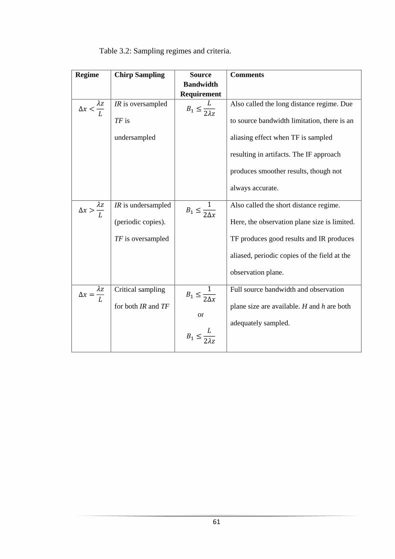
61
Table 3.2: Sampling regimes and criteria.
Regime Chirp Sampling Source
Bandwidth
Requirement
Comments
∆𝑥 <𝜆𝑧
𝐿
IR is oversampled
TF is
undersampled
𝐵1 ≤𝐿
2𝜆𝑧
Also called the long distance regime. Due
to source bandwidth limitation, there is an
aliasing effect when TF is sampled
resulting in artifacts. The IF approach
produces smoother results, though not
always accurate.
∆𝑥 >𝜆𝑧
𝐿
IR is undersampled
(periodic copies).
TF is oversampled
𝐵1 ≤1
2∆𝑥
Also called the short distance regime.
Here, the observation plane size is limited.
TF produces good results and IR produces
aliased, periodic copies of the field at the
observation plane.
∆𝑥 =𝜆𝑧
𝐿
Critical sampling
for both IR and TF
𝐵1 ≤1
2∆𝑥
or
𝐵1 ≤𝐿
2𝜆𝑧
Full source bandwidth and observation
plane size are available. H and h are both
adequately sampled.

62
3.1.5.3.2 Design Steps for Propagation Simulation
When simulating beam propagation, the following design steps should be considered [52].
Step 1: Ensure that the source support is at most 2 or 3 times less than the array side
length.
Step 2: Work out the Sampling regime; find out the corresponding propagator that
would suit.
Step 3: Consider the source bandwidth criteria.
Step 4: Observe the results and bandwidth, then reconsider source sampling.

63
3.2 Atmospheric Turbulence
As a result of differential heating and cooling of the earth by sunlight and diurnal cycles,
the temperature of the atmosphere is known to fluctuate randomly. This results in
random changes in wind velocity (as air moves, it transitions from a more uniform
pattern called Laminar flow to Turbulent flow, where the velocity field is no longer
uniform). The turbulent velocity field acquires randomly distributed pockets of air
called eddies which fluctuate in size and temperature causing corresponding variations
in the refractive index. These changes in refractive index act like lenses (of the size of
the eddy that caused it) in the atmosphere to focus and redirect the wavefront of incident
beam causing intensity variations. When the refractive index variations accumulate, it
can distort the wavefront of a beam propagating through the atmosphere [71,72].
3.2.1 The Structure of Atmospheric Turbulence
The history of the study of turbulences began with its recognition as a distinct
phenomenon by da Vinci in the 19th century. Due to the complexity of the atmosphere,
the concept of predicting atmospheric turbulence is not based on deterministic
prediction but based on statistical analysis. Turbulent flow is a nonlinear phenomenon
known to be governed by Navier- Stokes equations. Due to the complexity of solving
the Navier- Stokes equations for fully developed turbulence, Kolmogorov [ 73 , 74 ]
proposed statistical approximations of the [Navier-Stokes] equations. His theory is
among the most widely accepted and most consistent with experimental observations.
He submitted that the kinetic energy in large eddies is transferred into smaller eddies, in
turbulent flow. The average size of the largest eddies is called the outer scale L0 and
that of the smallest eddies is called inner scaler l0. The outer scale is the size above

64
which isotropic behaviour is violated and the inner scale is the size below which viscous
effects are important [72]. The average size of the inner scale 𝑙0 can be a few millimetres
near the ground to a few centimetres high above the ground. The outer scale 𝐿0 near the
ground is on the order of the height above the ground, and up to tens to hundreds of
metres high above the ground [75].The interval of eddy sizes between L0 and l0 is called
the inertial subrange.
In his analysis, Kolmogorov used the structure function instead of the more common
co-variance. This is because he made the assumption that eddies within the inertial
subrange are statistically isotropic and homogenous within small areas of space, and this
implies that their velocity and refractive index will not be incrementing with those areas
of space. Another assumption made is that the atmospheric turbulence is incompressible.
Based on these three assumptions, the structure tensor [72,76,77] Dij between any two
points in space separated by vector r:
𝐷𝑖𝑗 = ⟨[𝑣𝑖(𝐫𝐢 + 𝐫) − 𝑣𝑖(𝐫𝟏)] [𝑣𝑗(𝐫𝟏 + 𝐫) − 𝑣𝑗(𝐫𝟏)]⟩ (3.73)
is reduced to the following structure function, for the sake of simplicity:
𝐷𝑣 = ⟨[𝑣𝑟(𝐫𝟏 + 𝐫) − 𝑣𝑟(𝐫𝟏)]2⟩ (3.74)
The brackets represent an ensemble average and the vi and vj are the velocity
components. If we consider a case where the separation r is small and within the inertial
sub-range of turbulence (𝑙0 < 𝑟 < 𝐿0), the structure function becomes:
𝐷𝑣 = 𝐶𝑣2𝑟2 3⁄ (3.75)

65
where 𝐶𝑣2 is the velocity structure constant which is a measure of the energy in the
turbulence.
The velocity structure function has also been related to the refractive index, called the
Kolmogorov’s Sub-range Expression and is given as [78, 79]:
𝐷𝑛(𝑟) = 𝐶𝑛2 𝑟2 3⁄ for 𝑙𝑜 ≪ 𝑟 ≪ 𝐿𝑜
(3.76)
where 𝐶𝑛2 = refractive index structure constant, which is a measure of the strength of
turbulence.
3.2.2 Power Spectral Density of Refractive Index
It is assumed that the atmosphere is made up of two parts of refractive index: a mean
refractive index ⟨𝑛(𝐫)⟩ and a fluctuating refractive index part 𝑛1(𝐫). The covariance of
the refractive index field 𝐵𝑛 will be [72]:
𝐵𝑛 = ⟨𝑛1(𝐫 + 𝐫𝟏)𝑛1(𝐫𝟏)⟩
(3.77)
The Fourier transform of the covariance is known to give Power Spectral Density (PSD).
Hence, the power spectral density of the above covariance of refractive index is given
by:
Φ𝑛(𝐊) =1
(2𝜋)3∫ 𝑑3𝑟𝐵𝑛(𝑟)𝑒−𝑖𝐊 . 𝐫
(3.78)
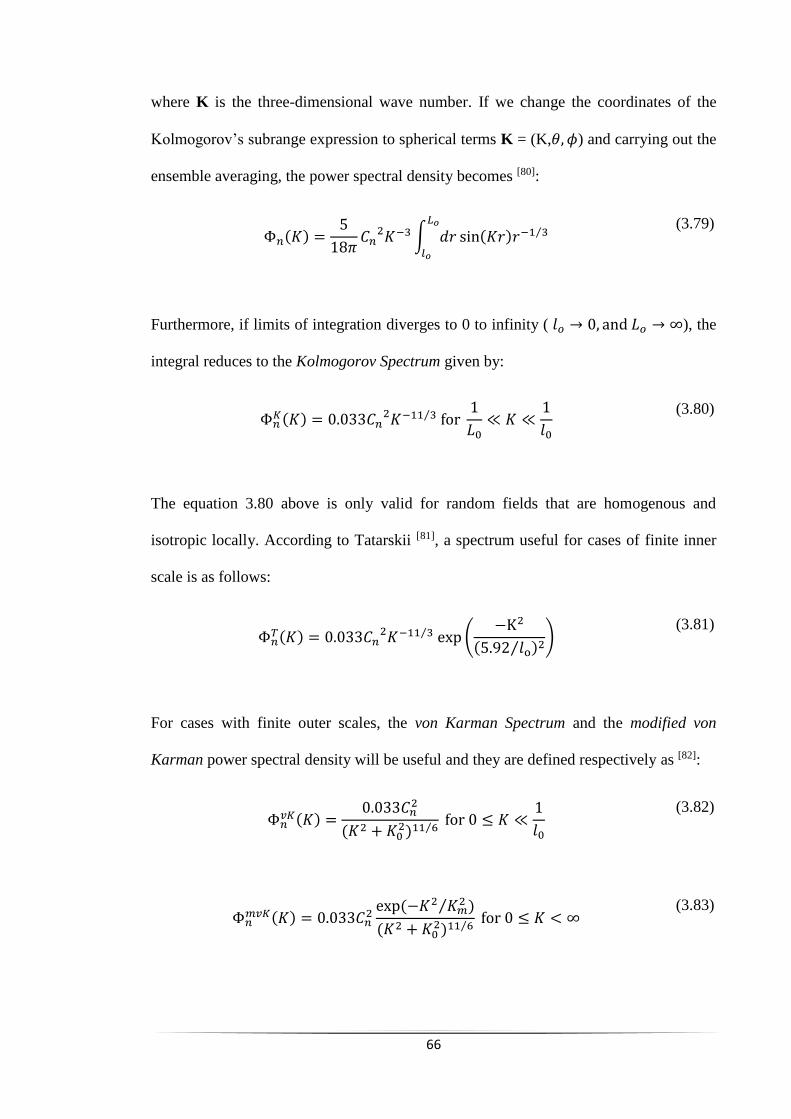
66
where K is the three-dimensional wave number. If we change the coordinates of the
Kolmogorov’s subrange expression to spherical terms K = (K,𝜃, 𝜙) and carrying out the
ensemble averaging, the power spectral density becomes [80]:
Φ𝑛(𝐾) =5
18𝜋𝐶𝑛
2𝐾−3 ∫ 𝑑𝑟𝐿𝑜
𝑙𝑜
sin(𝐾𝑟)𝑟−1 3⁄
(3.79)
Furthermore, if limits of integration diverges to 0 to infinity ( 𝑙𝑜 → 0, and 𝐿𝑜 → ∞), the
integral reduces to the Kolmogorov Spectrum given by:
Φ𝑛𝐾(𝐾) = 0.033𝐶𝑛
2𝐾−11 3⁄ for 1
𝐿0≪ 𝐾 ≪
1
𝑙0
(3.80)
The equation 3.80 above is only valid for random fields that are homogenous and
isotropic locally. According to Tatarskii [81], a spectrum useful for cases of finite inner
scale is as follows:
Φ𝑛𝑇(𝐾) = 0.033𝐶𝑛
2𝐾−11 3⁄ exp (−K2
(5.92 𝑙o⁄ )2)
(3.81)
For cases with finite outer scales, the von Karman Spectrum and the modified von
Karman power spectral density will be useful and they are defined respectively as [82]:
Φ𝑛𝑣𝐾(𝐾) =
0.033𝐶𝑛2
(𝐾2 + 𝐾02)11 6⁄
for 0 ≤ 𝐾 ≪1
𝑙0
(3.82)
Φ𝑛𝑚𝑣𝐾(𝐾) = 0.033𝐶𝑛
2exp (−𝐾2 𝐾𝑚
2⁄ )
(𝐾2 + 𝐾02)11 6⁄
for 0 ≤ 𝐾 < ∞
(3.83)

67
where 𝐾0 = 2𝜋 𝐿0⁄ and 𝐾𝑚 = 5.92 𝑙0⁄ and their values are chosen to match the small
scale and large scale behaviour predicted by the dimensional analysis [71]. Amongst all
the power spectral density models, the modified von Karman is the simplest that
includes the effects of both inner and outer scales [83].
3.2.3 Strength of Turbulence, Cn2
The strength of Atmospheric Turbulence which is characterised by the refractive index
structure constant, Cn2 in 𝑚−2 3⁄ . Cn
2 is not a constant as it sounds but it is a variable
entity by all means. Several experiments have been carried out over the years to confirm
that Cn2 changes with time of the day [84], location [85] as well as with altitude [86].
3.2.3.1 Variation with Altitude
Based on altitude, Cn2 is prevalent in the lower atmosphere due to more fluctuations in
refractive index of air and it diminishes with altitude. Typical values of Cn2 ranges from
10-13 to 10-18 m-2/3, with weak turbulence falling within the range 𝐶𝑛2 ≤ 10−17, moderate
turbulence 10−17 ≤ 𝐶𝑛2 ≤ 10−14 and strong turbulence 𝐶𝑛
2 ≥ 10−14 [87]. Hufnagel [88]
was one of the first to make experimental observations on the variation of Cn2 with
height in meters above the ground, h. He suggested that:
𝐶𝑛2(ℎ) = {[(2.2 × 10−53)ℎ10 (
𝑊
27)
2
] 𝑒−ℎ 1000⁄ + 10−16𝑒−ℎ 1500⁄ } exp[𝑟(ℎ, 𝑡)] (3.84)
where the 𝑟(ℎ, 𝑡) is a zero mean homogenous Gaussian random variable and W is the
wind correlating factor given as
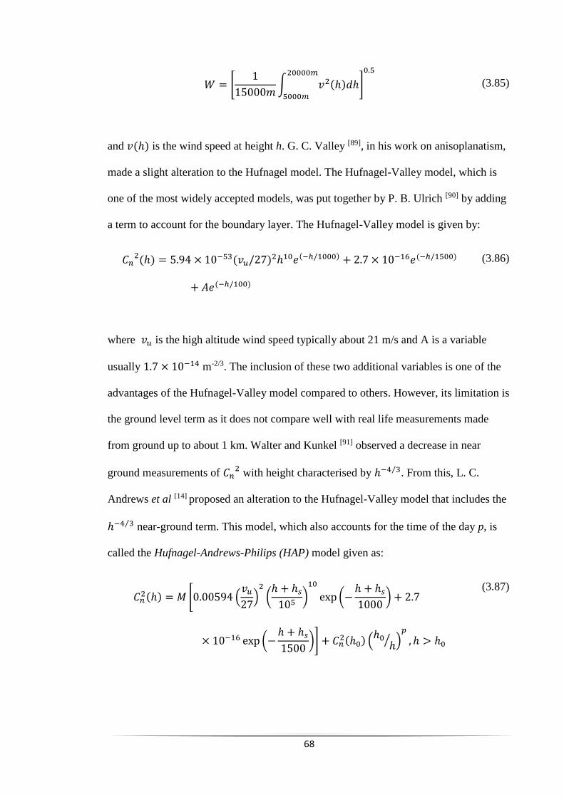
68
𝑊 = [1
15000𝑚∫ 𝑣2(ℎ)𝑑ℎ
20000𝑚
5000𝑚
]
0.5
(3.85)
and 𝑣(ℎ) is the wind speed at height h. G. C. Valley [89], in his work on anisoplanatism,
made a slight alteration to the Hufnagel model. The Hufnagel-Valley model, which is
one of the most widely accepted models, was put together by P. B. Ulrich [90] by adding
a term to account for the boundary layer. The Hufnagel-Valley model is given by:
𝐶𝑛2(ℎ) = 5.94 × 10−53(𝑣𝑢/27)2ℎ10𝑒(−ℎ/1000) + 2.7 × 10⁻¹⁶𝑒(−ℎ/1500)
+ 𝐴𝑒(−ℎ/100)
(3.86)
where 𝑣𝑢 is the high altitude wind speed typically about 21 m/s and A is a variable
usually 1.7 × 10⁻¹⁴ m-2/3. The inclusion of these two additional variables is one of the
advantages of the Hufnagel-Valley model compared to others. However, its limitation is
the ground level term as it does not compare well with real life measurements made
from ground up to about 1 km. Walter and Kunkel [91] observed a decrease in near
ground measurements of 𝐶𝑛2 with height characterised by ℎ−4 3⁄ . From this, L. C.
Andrews et al [14] proposed an alteration to the Hufnagel-Valley model that includes the
ℎ−4 3⁄ near-ground term. This model, which also accounts for the time of the day p, is
called the Hufnagel-Andrews-Philips (HAP) model given as:
𝐶𝑛2(ℎ) = 𝑀 [0.00594 (
𝑣𝑢
27)
2
(ℎ + ℎ𝑠
105)
10
exp (−ℎ + ℎ𝑠
1000) + 2.7
× 10−16 exp (−ℎ + ℎ𝑠
1500)] + 𝐶𝑛
2(ℎ0) (ℎ0
ℎ⁄ )
𝑝
, ℎ > ℎ0
(3.87)
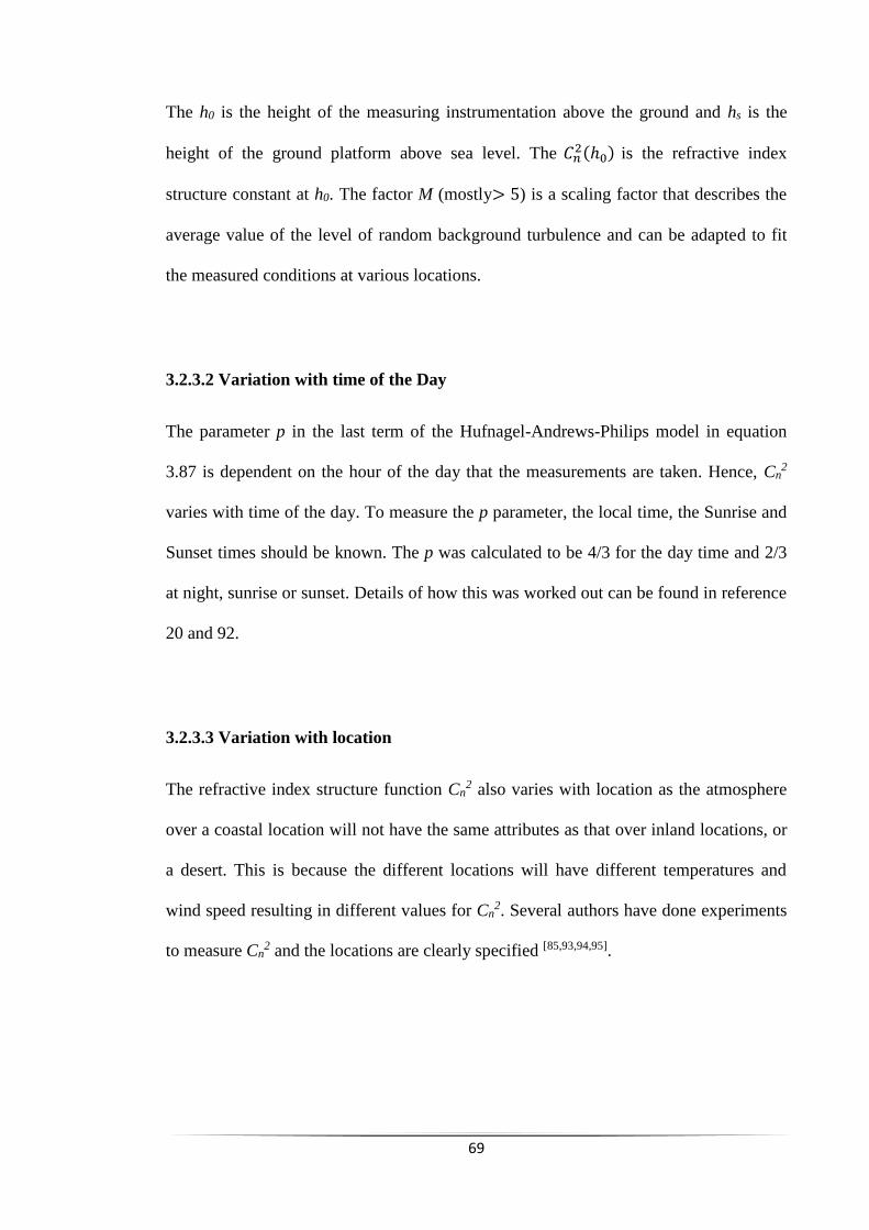
69
The h0 is the height of the measuring instrumentation above the ground and hs is the
height of the ground platform above sea level. The 𝐶𝑛2(ℎ0) is the refractive index
structure constant at h0. The factor M (mostly> 5) is a scaling factor that describes the
average value of the level of random background turbulence and can be adapted to fit
the measured conditions at various locations.
3.2.3.2 Variation with time of the Day
The parameter p in the last term of the Hufnagel-Andrews-Philips model in equation
3.87 is dependent on the hour of the day that the measurements are taken. Hence, Cn2
varies with time of the day. To measure the p parameter, the local time, the Sunrise and
Sunset times should be known. The p was calculated to be 4/3 for the day time and 2/3
at night, sunrise or sunset. Details of how this was worked out can be found in reference
20 and 92.
3.2.3.3 Variation with location
The refractive index structure function Cn2 also varies with location as the atmosphere
over a coastal location will not have the same attributes as that over inland locations, or
a desert. This is because the different locations will have different temperatures and
wind speed resulting in different values for Cn2. Several authors have done experiments
to measure Cn2 and the locations are clearly specified [85,93,94,95].
70
3.2.4 Coherence parameter, r0 and Phase Power Spectral Density
Cn2 is commonly used to compute other more useful parameters that are also measurable,
like the atmospheric coherence diameter or coherence parameter or Fried parameter, r0.
Coherence Diameter was first proposed by D. L. Fried [96] hence it’s popular name Fried
parameter. It can be defined as a degree of the quality of the optical propagation through
the atmosphere due to inhomogeneity and inconsistency in the refractive index of the
atmosphere. In other words, the coherence parameter can be seen as the diameter of a
circular area over which the rms aberration of a wavefront due to its propagation
through the atmosphere, is equal to 1 radian.
The Fried parameter is related to the variable Cn2 for a plane wave source with receiver
h distance away, as follows:
𝑟0,𝑝𝑤 = [0.423𝑘2 ∫ 𝐶𝑛2(ℎ)𝑑ℎ
ℎ
0
]
−3/5
(3.88)
For spherical wave point source, the Fried parameter is given as:
𝑟0,𝑠𝑤 = [0.423𝑘2 ∫ 𝐶𝑛2(ℎ) (
∆ℎ
ℎ)
5/3
𝑑ℎ
ℎ
0
]
−3/5
(3.89)
Typical values for Fried parameter r0 for visible wavelengths is known to be about 5 to
10 cm. Since r0 incorporates Cn2, propagation distance and wavelength in one
expression, it is more widely used to characterise atmospheric phenomena [72].
71
The refractive index Power Spectral Densities defined in section 3.22 in terms of Cn2
can now be redefined in terms of r0. But before this, the phase Power Spectral Density
Φ𝜙(𝐾), which is the form that will be needed in generating phase screens subsequently,
can be defined in terms of the refractive index Power spectral density Φ𝑛(𝐾) for a plane
wave as [71]:
Φ𝜙(𝐾) = 2𝜋2𝑘2∆𝑧Φ𝑛(𝐾)
(3.90)
Hence the phase Power Spectral Densities for the Kolmogorov, von Karman PSD and
the modified von Karman’s models are as follows:
Φ∅𝑘 = 0.49𝑟0
−5/3𝑘−11/3
(3.91)
Φ∅𝑣𝑘 =
0.49𝑟0−5/3
(𝑘2 + 𝑘02)11/6
(3.92)
Φ∅𝑚𝑣𝑘 = 0.49𝑟0
−5/3exp (−𝑘2/𝑘𝑚
2)
(𝑘2 + 𝑘02)11/6
(3.93)
3.2.5 Optical propagation through turbulence
As earlier mentioned, the wave equation derived in section 3.1.2 describes the
propagation of light signal both in a vacuum. This can also be used to describe the
additional effect of atmospheric turbulence present in the medium. Jason Schmidt [71] as
well as Andrews and Philips [83] derived this starting from wave equation for the electric
field given as:
∇2𝐄(𝐫) + 𝑘2𝑛2(𝐫) + 2∇[𝐄(𝐫). ∇In 𝑛(𝐫)] = 0 (3.94)
72
The term 2∇[𝐄(𝐫). ∇In 𝑛(𝐫)] stands for the change in polarisation of the wave as it
propagates. However when the wavelength is smaller than the inner scale ( 𝜆 < 𝑙0), the
wave equation is simplified to:
[∇2 + 𝑘2𝑛2(𝐫)]𝐄(𝐫) = 0
(3.95)
where E is the electric field vector and k is the vacuum wavenumber, n is the refractive
index. Since magnetic induction B also has the same relationship, the equation can be
presented in a general form to cover all field components:
[∇2 + 𝑘2𝑛2(𝐫)]𝑈(𝐫) = 0
(3.96)
The refractive index in equation 3.96 above is position-dependent, and that is what
makes it different from equation 3.22. To solve the equation 3.96, we assume a weak
fluctuation condition which means that equation 3.77 becomes
𝑛2(𝐫) ≅ 1 + 2𝑛1(𝐫)
(3.97)
When this is substituted into the wave equation in equation 3.96, it becomes:
{∇2 + 𝑘2[1 + 2𝑛1(𝐫)]}𝑈(𝐫) = 0
(3.98)
This equation is solved by Fourier optics when the refractive index in the medium is
constant. But the atmosphere is typically not homogenous and the refractive index is not
constant. Hence the Fourier optics method is used along with some perturbative

73
methods to derive approximate solutions. The vacuum solution 𝑈0(𝐫) to the equation
3.98 is one of the parameters of the optical field 𝑈(𝐫) in the Rytov [97] method given by:
𝑈(𝐫) = 𝑈0(𝐫)exp [𝜓(𝐫)]
(3.99)
The 𝜓(𝐫) is the complex phase perturbation. When the amplitude and phase quantities
are isolated, it is written as:
𝜓 = 𝜒 + 𝑖𝜙
(3.100)
where 𝜒 is the log-amplitude perturbation and 𝜙 is the phase perturbation induced by
the turbulence. More details of these two quantities are discussed in the section 3.2.6.
3.2.6 Propagation Defects of turbulence
When an optical beam is propagated through atmospheric turbulence, there are three
categories of propagation defects known to happen to the beam namely beam wander,
beam spreading and intensity fluctuations. The intensity variations, usually expressed as
the log-amplitude fluctuations, are caused by eddies with the size on the order of
(𝜆𝐿)1 2⁄ . The eddies that are large compared with the beam radius tend to deflect the
beam; this is called Beam Wander. The eddies that are small compared with the beam
radius do not deflect the beam much but tend to broaden the beam; this is called Beam
spread [80]. The details of these defects come in the next three subsections.

74
3.2.6.1 Intensity Variation
An optical beam propagating through atmospheric turbulence, even over short paths,
will definitely experience intensity fluctuations. All experimental and theoretical
research on intensity fluctuations usually centres around the normalised variance of the
intensity fluctuations, called Scintillation index and is defined by [98]:
𝜎𝜒2 =
⟨𝐼2⟩ − ⟨𝐼⟩2
⟨𝐼⟩2=
⟨𝐼2⟩
⟨𝐼⟩2− 1
(3.101)
where the angle brackets ⟨ ⟩ denotes ensemble average, I is the intensity of the optical
beam. The Scintillation index is dimensionless. Scintillation levels are divided into three
categories [ 99 ], depending on the scintillation index: the weak intensity-fluctuation
regime with 𝜎𝜒2 < 0.3, the medium regime with 0.3 ≤ 𝜎𝜒
2 < 5 and the strong
fluctuations or saturation regime with 𝜎𝜒2 ≥ 5. In the weak fluctuations regime, the
scintillation index of an unbounded plane wave based on the Kolmogorov spectrum is
called the Rytov variance given by: [72,79,97]:
𝜎𝜒2 = 1.23𝑘7 6⁄ 𝐿11 6⁄ 𝐶𝑛
2 (3.102)
while the log-amplitude fluctuation variance for a spherical wave is:
𝜎𝜒2 = 0.124𝑘7 6⁄ 𝐿11 6⁄ 𝐶𝑛
2
(3.103)
The above two log-amplitude fluctuation expressions in equations 3.102 and 3.103 were
derived from perturbation theory hence they break down for long paths and strong
turbulence. Since eddies are considered to act as lenses, the focal length of an eddy of
diameter 𝑙 will be 𝑓 ≅ 𝑙 ∆𝑛⁄ , where ∆𝑛 is the difference in refractive index. In the
75
geometric optical domain (where 𝑙 > √𝜆𝐿 and 𝑙𝑜 < √𝜆𝐿 ), Clifford [100] expresses the
log-amplitude variance as:
𝜎𝜒2~𝑘7 6⁄ 𝐿11 6⁄ 𝐶𝑛
2
(3.104)
where L is the propagation path length.
More authors [ 101 , 102 ] have conducted experiments to measure Scintillation index,
verifying that experimental results deviate from these theoretical predictions, as well as
that the Scintillation index near the diffractive end of the collimated beam was
considerably larger than the on-axis values. Optical scintillation can be reduced by
aperture averaging [ 103 ]; increasing the collecting area of the receiver lens by the
integral of all the components of the incident intensity on a particular part of the lens
[104].
3.2.6.2 Phase Variation
Random variation in phase causes waveform distortion as mentioned earlier. These
phase variations, mostly measured with an interferometer, is as a result of the refractive
index being a random function of space and time. In practice, the distortion caused by
intensity variations is small compared to that caused by phase variations [105]. When two
parallel optical wave paths separated by a distance 𝜌 propagate through space, the phase
difference 𝛿𝜙 between them is given by [72]:
𝛿𝜙 ≅ 𝑘𝜌[Δ𝑛(𝜌)]
(3.105)
76
In their study, Clifford [106] et al defined the phase structure function as:
𝐷𝜙 = ⟨[𝜙(𝐫 + 𝜌) − 𝜙(𝐫)]2⟩
(3.106)
Again here, the angle brackets indicate ensemble average. The phase structure function
is necessary for defining the phase coherence. After averaging over many statistical
realizations, Tatarskii [79] defines phase structure function for plane waves as:
𝐷𝜙(𝜌) = 2.91𝑘2𝐿𝐶𝑛2𝜌5 3⁄ , for √𝜆𝐿 ≤ 𝜌 < 𝐿0
(3.107)
and that for spherical waves as:
𝐷𝜙(𝜌) = 1.09𝑘2𝐿𝐶𝑛2𝜌5 3⁄ , for √𝜆𝐿 ≤ 𝜌 < 𝐿0
(3.108)
The wave is most likely to lose coherence when it is propagated over long paths and
over many eddies. The beam becomes coherent only if the phase difference ⟨(𝛿𝜙)2⟩ <
𝜋2. Substituting this condition for coherence into equation 3.107 above, the coherent
distance 𝜌𝑜 (largest eddy for which a plane is considered coherent) is obtained as [72]:
𝜌𝑜 = [𝜋2
𝑘2𝐶𝑛2𝐿
]
3 5⁄
(3.109)
Hence, when two optical beams or two parts of the same beam propagate through the
same distance L of atmospheric turbulence, though they may arrive at the same point,
they arrive using a slightly different path and have different angles of arrival. Kon and
Tatarskii [107] defines the variance of their angle of arrival difference as
⟨𝛼2⟩ =𝐷𝜙
𝑘2𝜌2
(3.110)

77
where the 𝐷𝜙is the phase structure function for plane waves. For an aperture of diameter
D, the angle of arrival variance becomes:
⟨𝛼2⟩ = 2.91𝐶𝑛2𝐿𝐷−1 3⁄
(3.111)
This variance in angle of arrival in equation 3.111 above is the quantity that measures
Beam Wander: a random displacement of the received beam’s focal spot from the
centroid coordinate.
3.2.6.3 Beam Spread for Coherent Beam
Optical beams are known to spread out as they propagate, even without the additional
effect of turbulence. This is primary as result of diffraction, resulting in the beam radius
gradually increasing and the beam energy gradually weakening as it propagates. This
effect was discussed in section 2.1. The beam spread is also made more severe with the
additional effect of atmospheric turbulence. The constraint for coherence distance in
equation 3.109 can be used to define the total beam spread as well. In an ideal case of
constant turbulence 𝐶𝑛2 regardless of altitude, the angular spread 𝜃 for a collimated
uniform beam of radius 𝜔 in uniform turbulence is given by [108]:
𝜃2 ≅1
𝑘2𝜔2+
1
𝑘2𝜌𝑜2
(3.112)
For a typical Gaussian beam whose intensity profile is defined by the function below
(same as equation 2.9), with an initial beam waist diameter 𝑤𝑜:
𝐼 =𝑤𝑜
2
𝑤𝑏2
exp (−2𝜌2
𝑤𝑝2
)
(3.113)
78
When the Gaussian beam is propagated for long distances (z ≫ π𝑤𝑜2/𝜆), the beam
waist will spread to:
𝑤𝑏2 =
4𝑧2
𝑘2𝑤𝑜2
+ 3.58𝐶𝑛2𝐿3𝑤𝑜
−1 3⁄
(3.114)
When propagated for a short distance (z ≪ π𝑤𝑜2/𝜆), the waist becomes:
𝑤𝑏2 = 𝑤𝑜
2 + 2.86𝐶𝑛2𝑘1 3⁄ 𝐿8 3⁄ 𝑤𝑜
1 3⁄
(3.115)
3.2.7 Turbulence Phase Screen
It is important to be able to model properly the random turbulence in the lower
atmosphere, in order to have an accurate FSO propagation simulation. For the purpose
of simplification of analytical calculations and computer simulations, the technique
commonly used to model atmospheric turbulence is to consider it as a finite number of
discrete layers [109,110]. Each of the layers is a thin (its thickness is much less than the
propagation distance that follows [111]) phase screen used to represent a much thicker
volume of turbulence. In theory, the turbulence profile in the ith phase screens is in
terms of the effective strength of turbulence 𝐶𝑛2
𝑖, the thickness of the turbulence ∆𝑧𝑖
and the location of the phase screen along the propagation path 𝑧𝑖 [71]. The phase screens
are imaginarily placed at intervals through the lower atmosphere. The common process
of propagation through turbulence phase screens is the Split-step beam propagation
method [112,113].
Over the years, different methods have been used to model the phase screens like the
Zernike polynomial method [114], covariance method [115], Discrete Fourier Transform
method [116]. Although these different methods do have their own pros and cons, the

79
Fourier Transform method is most commonly used because of its computational
efficiency. Its major drawback is inaccuracy due to the undersampling of the low spatial
frequency, where most of the power reside. Several methods have been proposed to
compensate for these deficient low frequency components, one of them is called the
Subharmonic method [117,118]. The Subharmonic method was later validated to be
accurate by Frehlich [119].
Phase screens are created by transforming random numbers generated on the computer
into 2D arrays of phase values on a grid of sample points having the same statistical
properties as the turbulence-induced phase variations [71]. For a finite square grid, the
Fourier Transform-based phase screen is generated using the expression below [119, 120]:
∅(𝑥, 𝑦) = ∑ ∑ [𝑅(𝑁) + i𝑅(𝑁)] × √Φ𝜙 ×
∞
𝑚=−∞
∞
𝑛=−∞
exp [𝑖2𝜋(𝑓𝑥𝑛𝑥 + 𝑓𝑦𝑚
𝑦)] (3.116)
where R represents Gaussian random numbers with zero mean and unit variance. N is
the number of grid points per side of the screen, 𝑓𝑥𝑛and 𝑓𝑦𝑚
are the discrete spatial
frequencies in the x and y directions. As earlier stated, the phase screen generated from
equation 3.116 above is deficient in the low spatial frequencies and this is augmented
using the method proposed by Lane et al [117]. Also from equation 3.116 above, 𝛷𝜙 is
the phase Power Spectral Density (PSD) of turbulence. This term characterises the
turbulence and it is based on refractive index variations. Different phase PSD models
have been defined earlier in section 3.2.4.
80
To supplement the low frequency components in the Fourier transform method, a low
frequency screen is generated as a sum of Np different screens given by [71,117]:
∅𝑙𝑓(𝑥, 𝑦) = ∑ ∑ ∑ 𝐶𝑛,𝑚exp [𝑖2𝜋(𝑓𝑥𝑛𝑥 + 𝑓𝑦𝑚
𝑦)]
1
𝑚=−1
1
𝑛=−1
𝑁𝑝
𝑝=1
(3.117)
where n and m are discrete frequencies and each p represents the different grids. The
𝐶𝑛,𝑚 are the random draws of the Fourier series coefficients.
3.2.8 Split-Step Propagation method
The method commonly used for optical beam propagation through atmospheric
turbulence is the split-step propagation method. This method, which was first
introduced by Tappert and Hardin [121], is a pseudo-spectral method that entails logically
breaking the propagation path length into equal intervals, say Δ𝑧. The main advantage
of this method, compared to other methods which are mostly time-domain finite
difference methods, is speed and ease of implementation. The first step in this split-step
method is to make an axial advance, propagating the initial beam forward by Δ𝑧 using
one of the propagators defined in section 3.1.4. Then the phase screen is applied in the
coordinate space before another axial advance of Δ𝑧 is made using the propagator. This
continues until the whole propagation path length is covered. It should be noted that the
phase screens do not need to be applied at every axial advance made and the interval
between applications of the phase screens is expected to satisfy the condition [12]:
𝐿0 ≪ ∆𝑧 ≪ 𝐿𝑑
(3.117)
where 𝐿𝑑 is the diffraction length or Rayleigh length.
81
3.3 Chapter Summary
In this chapter, we discussed the fundamental theory behind the propagation of the
Gaussian and Bessel beams through atmospheric turbulence. In the first section of the
chapter, we did a thorough literature review of Fourier Optics, treating the Maxwell’s
equations and deriving the wave equations as well as the Helmholtz equation. We went
on to discuss the Fourier Analysis, looking at the definitions of both the analytical and
the Discrete Fourier Transforms as well as the Fourier transform theorems. We
reviewed the Scalar Diffraction theory: the Huygens-Fresnel Principle, the Fresnel and
Fraunhofer diffraction approximations. Then we did a detailed discussion of the
sampling theory, covering the sampling regimes and criteria. The second section of the
chapter covers the theory of atmospheric turbulence, encapsulating the structure of
turbulence, the power spectral density of refractive index, the strength of turbulence, the
coherence (Fried) parameter, propagation defects of turbulence, the theory of turbulence
phase screens and Split-step propagation method which will be the method that will be
adopted in the beam propagation in chapters 5 and 6.

82
CHAPTER 4
83
4.0 MODELLING THE BEAMS AND THE ATMOSPHERIC TURBULENCE
This chapter describes our model for creating the Gaussian beam and Bessel beam,
which will be utilised in chapter 5 and 6. Here we model the power contained in the
beams. This will include deriving the minimum radii for the both beams, with their
respective altitudes, to ensure that not more than 50% of the initial beam power is lost
before it arrives at the receiver. The second section of this chapter will encapsulate the
modelling of the atmospheric turbulence as well as deriving the maximum height
beyond which the effect of turbulence is negligible.
4.1 Gaussian Beam Model
Many lasers available in the market produce beams that approximate a Gaussian profile,
a radially symmetrical distribution. In this section, we model the Gaussian beam that
will be propagated in chapter 5. A few mathematical system models will be derived to
help define the beam model. We also look at the power contained in the Gaussian beam
we are creating.
4.1.1 Creating the Gaussian Beam
The general form of the Gaussian beam is given in equation 4.1 below, similar to the
earlier defined equation 2.8, it is implemented in Matlab.
𝑈𝑔 = A exp (−𝑟2
𝜔02
) (4.1)
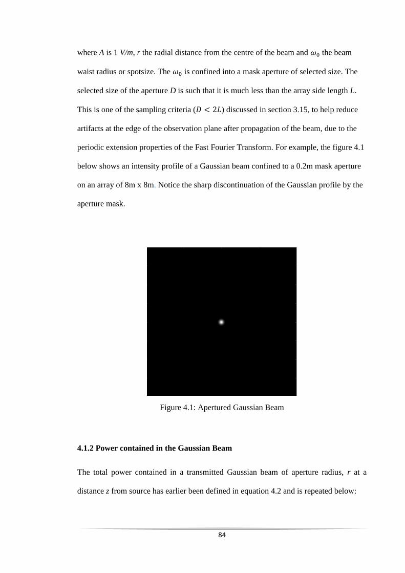
84
where A is 1 V/m, r the radial distance from the centre of the beam and 𝜔0 the beam
waist radius or spotsize. The 𝜔0 is confined into a mask aperture of selected size. The
selected size of the aperture D is such that it is much less than the array side length L.
This is one of the sampling criteria (𝐷 < 2𝐿) discussed in section 3.15, to help reduce
artifacts at the edge of the observation plane after propagation of the beam, due to the
periodic extension properties of the Fast Fourier Transform. For example, the figure 4.1
below shows an intensity profile of a Gaussian beam confined to a 0.2m mask aperture
on an array of 8m x 8m. Notice the sharp discontinuation of the Gaussian profile by the
aperture mask.
Figure 4.1: Apertured Gaussian Beam
4.1.2 Power contained in the Gaussian Beam
The total power contained in a transmitted Gaussian beam of aperture radius, r at a
distance z from source has earlier been defined in equation 4.2 and is repeated below:

85
𝑃 = 𝑃0 (1 − exp (−2𝑟2
𝑤(𝑧)2⁄ )) (4.2)
where 𝑃0 = 𝜋𝐼0𝑤02 2⁄ is the initial or total beam power at a beam radius 𝑤0 and 𝐼0 is the
peak intensity. Typically for a Gaussian beam transmitting through an aperture radius r
equal to the initial beam radius w0 (i.e. at z=0), 86.5% of its total power will be
transmitted according to equation 2.12. See section 2.12 for more details. To ensure that
99% of the initial beam power is transmitted, a transmitter aperture radius r of 1.5174𝑤0
is required. This condition was satisfied to ensure that the beam in figure 4.1 had 99%
of the energy passing through the aperture. If the receiver telescope also has aperture
radius equal to 1.5174𝑤0, 50% of the initial beam power will be lost at the receiver
when the received beam waist radius is:
𝑤(𝑧) = 2.5775𝑤0 (4.3)
and the distance that would be travelled for 50% of the initial power to be lost is given
by:
𝑧0.5𝑃 = 1.2560𝜋𝑤0
2
𝜆 (4.4)
From equation 4.4, the corresponding minimum initial beam wait radius required for 50%
of the initial power to be lost (when 99% was transmitted) can be derived as:
𝑤0.5𝑃 = 1.5174√𝑧𝜆
1.2560𝜋 (4.5)
The table 4.1 below shows a list of useful propagation targets for ground-to-space
Gaussian beam propagation. Here, it is assumed that the transmitter and receiver
telescopes both have the same aperture radius.
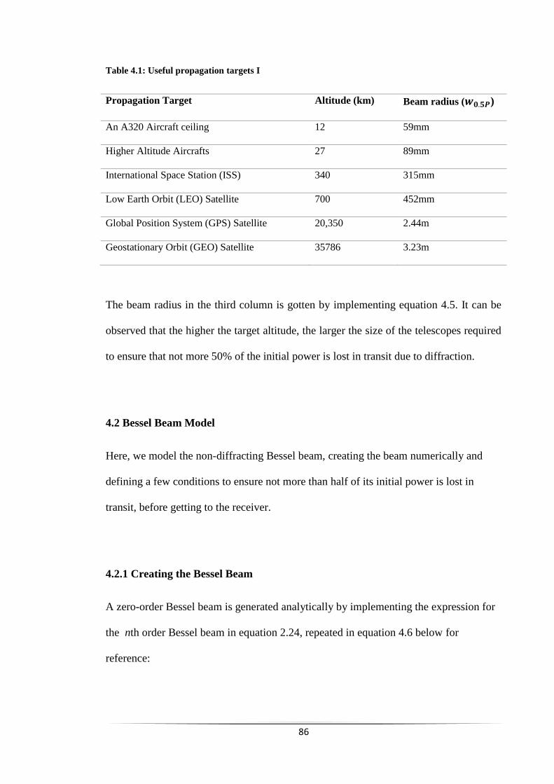
86
Table 4.1: Useful propagation targets I
Propagation Target Altitude (km) Beam radius (𝒘𝟎.𝟓𝑷)
An A320 Aircraft ceiling 12 59mm
Higher Altitude Aircrafts 27 89mm
International Space Station (ISS) 340 315mm
Low Earth Orbit (LEO) Satellite 700 452mm
Global Position System (GPS) Satellite 20,350 2.44m
Geostationary Orbit (GEO) Satellite 35786 3.23m
The beam radius in the third column is gotten by implementing equation 4.5. It can be
observed that the higher the target altitude, the larger the size of the telescopes required
to ensure that not more 50% of the initial power is lost in transit due to diffraction.
4.2 Bessel Beam Model
Here, we model the non-diffracting Bessel beam, creating the beam numerically and
defining a few conditions to ensure not more than half of its initial power is lost in
transit, before getting to the receiver.
4.2.1 Creating the Bessel Beam
A zero-order Bessel beam is generated analytically by implementing the expression for
the nth order Bessel beam in equation 2.24, repeated in equation 4.6 below for
reference:

87
𝐸(𝑟, 𝜙, 𝑧) = 𝐴0 exp(𝑖𝑘𝑧𝑧)𝐽0 (𝑘𝑟𝑟)exp (±𝑖𝑛𝜙) (4.6)
A Bessel beam is known to be ideal and in order to be generated, it has to be truncated
into an aperture function. The radial wave vector 𝑘𝑟 was derived in equation 2.28 as:
𝑘𝑟 =
2.405
𝐵𝑤 (4.7)
where 𝐵𝑤 is the radius of the circular aperture function placed on the beam. Like the
Gaussian beam, the size of the aperture D is also much less than the array side length L
to help reduce artifacts at the edge of the observation plane after propagation of the
beam. The 𝑘𝑟 is chosen such that the aperture 𝐵𝑤 is equal to the size of the Bessel
beam’s central core (its first zero), trimming off the outer rings, which would have
reflected off the walls of the observation grid and distort the beam. And since the
Gaussian beam generated in section 4.1.1 is also masked by an aperture function 𝑤0,
which is set to be equal to 𝐵𝑤, this ensures a fair basis of comparing the two beams as
proposed by Durnin in his comparison of these two beams. The 𝜙 is the argument of the
radial distance, r from the centre of the beam.
Another implication of trimming off the outer rings of the Bessel beam is a severe loss
in the beam energy as a significant part of the Bessel beam energy is carried in the outer
rings. Another effect of having to truncate the Bessel beam is that its non-diffracting
properties are only valid with the distance Zmax defined in equation 2.25, and rewritten
as:
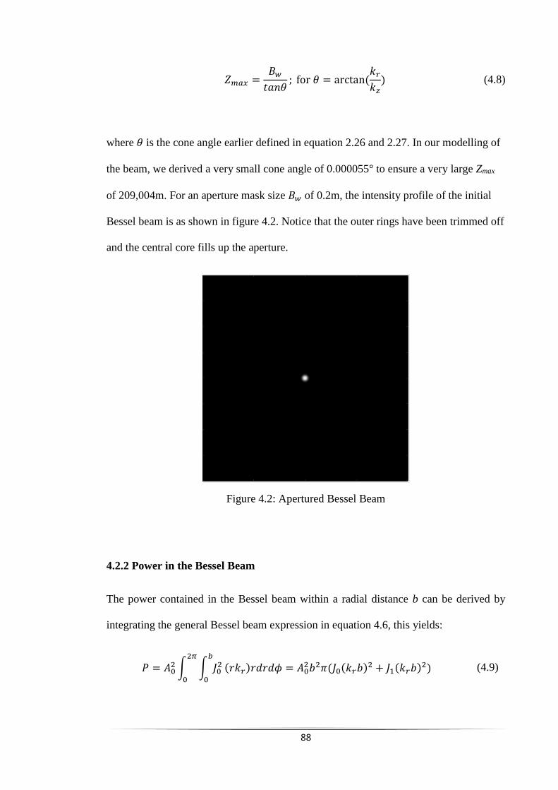
88
𝑍𝑚𝑎𝑥 =
𝐵𝑤
𝑡𝑎𝑛𝜃; for 𝜃 = arctan (
𝑘𝑟
𝑘𝑧) (4.8)
where 𝜃 is the cone angle earlier defined in equation 2.26 and 2.27. In our modelling of
the beam, we derived a very small cone angle of 0.000055° to ensure a very large Zmax
of 209,004m. For an aperture mask size 𝐵𝑤 of 0.2m, the intensity profile of the initial
Bessel beam is as shown in figure 4.2. Notice that the outer rings have been trimmed off
and the central core fills up the aperture.
Figure 4.2: Apertured Bessel Beam
4.2.2 Power in the Bessel Beam
The power contained in the Bessel beam within a radial distance b can be derived by
integrating the general Bessel beam expression in equation 4.6, this yields:
𝑃 = 𝐴02 ∫ ∫ 𝐽0
2𝑏
0
2𝜋
0
(𝑟𝑘𝑟)𝑟𝑑𝑟𝑑𝜙 = 𝐴02𝑏2𝜋(𝐽0(𝑘𝑟𝑏)2 + 𝐽1(𝑘𝑟𝑏)2) (4.9)
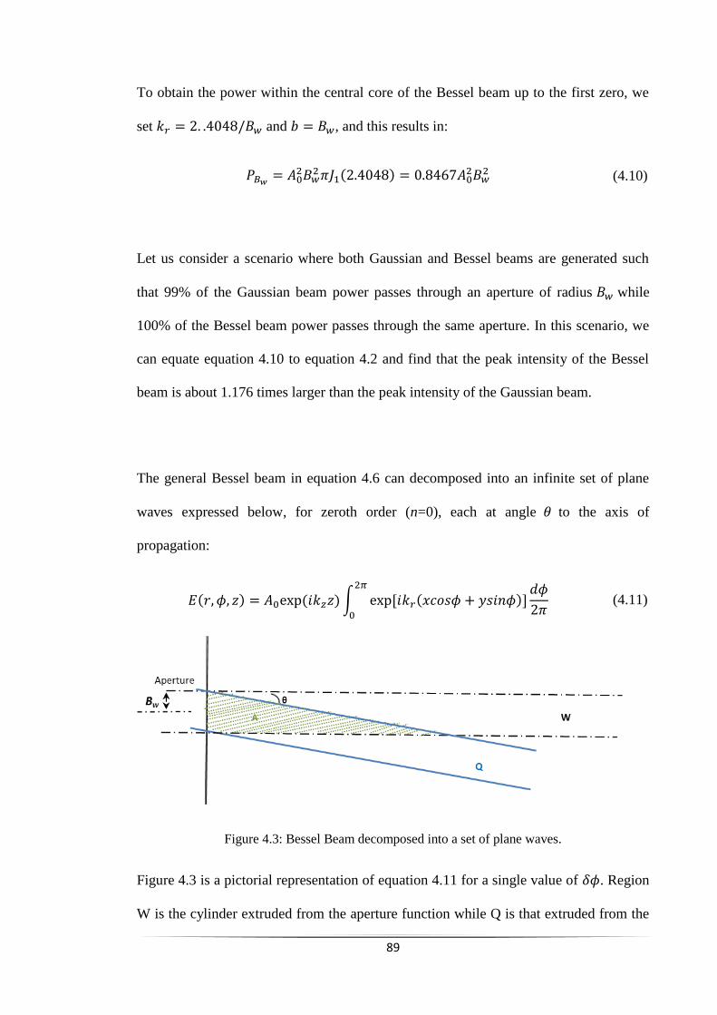
89
To obtain the power within the central core of the Bessel beam up to the first zero, we
set 𝑘𝑟 = 2. .4048/𝐵𝑤 and 𝑏 = 𝐵𝑤, and this results in:
𝑃𝐵𝑤= 𝐴0
2𝐵𝑤2 𝜋𝐽1(2.4048) = 0.8467𝐴0
2𝐵𝑤2 (4.10)
Let us consider a scenario where both Gaussian and Bessel beams are generated such
that 99% of the Gaussian beam power passes through an aperture of radius 𝐵𝑤 while
100% of the Bessel beam power passes through the same aperture. In this scenario, we
can equate equation 4.10 to equation 4.2 and find that the peak intensity of the Bessel
beam is about 1.176 times larger than the peak intensity of the Gaussian beam.
The general Bessel beam in equation 4.6 can decomposed into an infinite set of plane
waves expressed below, for zeroth order (n=0), each at angle 𝜃 to the axis of
propagation:
𝐸(𝑟, 𝜙, 𝑧) = 𝐴0exp (𝑖𝑘𝑧𝑧) ∫ exp [𝑖𝑘𝑟(𝑥𝑐𝑜𝑠𝜙 + 𝑦𝑠𝑖𝑛𝜙)]𝑑𝜙
2𝜋
2𝜋
0
(4.11)
Figure 4.3: Bessel Beam decomposed into a set of plane waves.
Figure 4.3 is a pictorial representation of equation 4.11 for a single value of 𝛿𝜙. Region
W is the cylinder extruded from the aperture function while Q is that extruded from the
90
plane wave. The shaded region, A (= Q ∩ W) is the region of no power loss as the beam
propagates. The energy contained within a single plane wavefront at angle 𝛿𝜙 is the
integral of the wavefront in the region A. The power contained in the W region can be
obtained by integrating over all the 𝜙:
𝑃(𝑧) = |∫ ∫ ∫ exp[𝑖𝑘𝑟(𝑥𝑐𝑜𝑠𝜙 + 𝑦𝑠𝑖𝑛𝜙)]𝑑𝜙
2𝜋𝑑𝑥𝑑𝑦
2𝜋
0𝐴
|
2
(4.12)
𝑃(𝑧) = |∬ 𝐽0(𝑘𝑟𝑟)d𝑥d𝑦𝐴
|
2
(4.13)
Some simulations were carried out to find out the distance at which half the power was
lost. This was obtained by implementing equation 4.13 as well as the Fresnel
propagation code, for a range of apertures 0.01 to 1 m. It was found that the half-power
distance appears to be at 𝑍𝑚𝑎𝑥. But when 𝑘𝑟 is assumed to be small such that the first
root of the beam is equal to the radius of the aperture function, the half-power distance
appears at about (1.1803532±0.0000067)𝑍𝑚𝑎𝑥.
Again, if we assume that the amplitude of the Bessel beam is zero at the edge of the
aperture function, we are able to derive an expression for the minimum beam radius,
from equation 4.7 and 4.8, expressed as:
𝐵𝑤𝑚𝑖𝑛 = √
2.405𝑍𝑚𝑎𝑥
𝑘 (4.14)

91
Recalling that when 𝑘𝑟 is small, the half-power distance is at approximately 1.18𝑍𝑚𝑎𝑥,
hence equation 4.14 becomes:
𝐵𝑤𝑚𝑖𝑛 = √
2.405𝑍𝑚𝑎𝑥
1.18𝑘
(4.15)
Table 2 shows another list of useful propagation targets, this time for Bessel beam
propagation from ground to space. Here, the third column is derived from equation 4.15,
which are the minimum radius of the transmit and receive telescopes required to ensure
that not more than half the power of the initial beam is lost.
Table 4.2: Useful propagation targets II
Propagation Target Altitude (km) Beam radius (𝑩𝒘𝒎𝒊𝒏)
An A320 Aircraft ceiling 12 44mm
Higher Altitude Aircrafts 27 77mm
International Space Station (ISS) 340 235mm
Low Earth Orbit (LEO) Satellite 700 337mm
Global Position System (GPS) Satellite 20,350 1.82m
Geostationary Orbit (GEO) Satellite 35786 2.41m
Clearly from table 4.2, larger diameters of telescopes are required for longer distance
propagation of Bessel beams. Compared to table 1, it can be seen that Gaussian beams
require larger diameters of telescopes to ensure not more than half the power is lost for
the same distance of propagation, compared to the Bessel beam which requires a smaller
transmitter size. This is the case because we have shown that to achieve maximum
propagation distance, the Bessel beam’s radial frequency kr needs to be chosen such that
the aperture function radius is equal to the first root of the Bessel function. Hence the
92
Bessel beam is more convenient than the Gaussian as it requires less weight, cost and
size.
4.3 Modelling the Atmospheric Turbulence
In this section, we will model the atmospheric turbulence in the medium. It is critical to
be able to model effectively the random turbulence in the atmosphere. As earlier
mentioned in section 3.2.8, the phase screen method is used here due to its simplicity
for analytical calculations and computer simulations. Here, a finite number of phase
screens are imaginarily placed at intervals through the atmosphere, in a split-step
method. In the split-step method, the entire propagation path is logically split into equal
intervals and the beam is hence propagated in intervals. The phase screens are applied at
every other interval, before the next advancement of the beam, and this continues till the
whole propagation path length is covered. The first subsection discusses our derived
model for the Cn2 with respect to altitude, from where we derive a maximum height
above which the effect of turbulence is considered negligible. The second subsection
summarises the generation of the phase screens.
4.3.1 Maximum Height for Turbulence
As established in section 3.2, the strength of atmospheric turbulence Cn2 is not fixed in
any way as it varies with altitude, location and time of the day. However, Cn2 is only
considered fixed when trying to model terrestrial (ground-to-ground) applications; but
for ground-to-space applications, it varies with height.
93
The Hufnagel-Valley’s model of Cn2 with respect to height h above the ground is one of
the most widely accepted. The Hufnagel-Andrews-Philips (HAP) model, earlier defined
in equation 3.87, is an efficient modification to the Hufnagel-Valley model and
accounts for time of the day, p. It is repeated below for reference:
𝐶𝑛2(ℎ) = 𝑀 [0.00594 (
𝑣𝑢
27)
2
(ℎ + ℎ𝑠
105)
10
exp (−ℎ + ℎ𝑠
1000) + 2.7
× 10−16 exp (−ℎ + ℎ𝑠
1500)] + 𝐶𝑛
2(ℎ0) (ℎ0
ℎ⁄ )
𝑝
, ℎ > ℎ0
(4.16)
Here, the h0 is the height of the measuring instrumentation above the ground and hs is
the height of the ground platform above sea level. The 𝐶𝑛2(ℎ0) is the refractive index
structure constant at h0. The factor M (mostly> 5) is a scaling factor that describes the
average value of the level of random background turbulence and can be suited to fit the
measured conditions at various locations. From the above HAP model in equation 4.16,
using the factor M = 6.5, and if the ground platform and measurement instrumentations
are assumed to be at sea level (hs and ho = 0), we derive a modification to the Cn2(h) as:
𝐶𝑛
2(ℎ) = 6.5 [3.593 × 10⁻³ (ℎ105⁄ )
10𝑒(−ℎ/1000) + 2.7 × 10⁻¹⁶𝑒(−ℎ/1500)] (4.17)
Given that typical values for Cn2 are known to be ranging from 10-13 to 10-18 m-2/3 , we
can deduce from equation 4.17 above that the maximum height above which Cn2 would
be lower than as 10-18 m-2/3 will be 22 km high. Based on our model, the range for 𝐶𝑛2 is
from 𝐶𝑛2(0) = 1.75× 10⁻¹⁵ to 𝐶𝑛
2(22𝑘𝑚) = 1.73 × 10⁻¹⁸. This means that there would be
negligible atmospheric turbulence at altitudes above 22km. This fact will be key when
simulating the optical beam propagation for a ground-to-space scenario as the
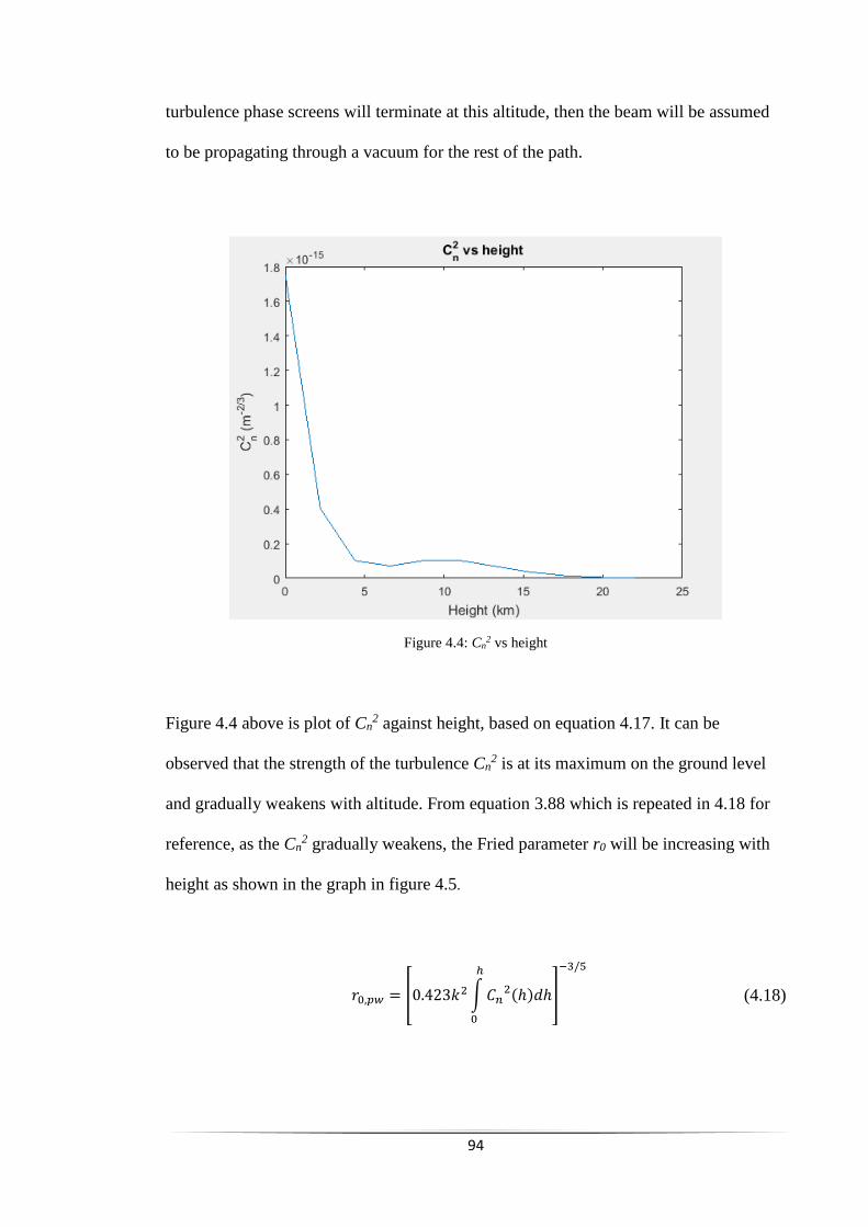
94
turbulence phase screens will terminate at this altitude, then the beam will be assumed
to be propagating through a vacuum for the rest of the path.
Figure 4.4: Cn2 vs height
Figure 4.4 above is plot of Cn2 against height, based on equation 4.17. It can be
observed that the strength of the turbulence Cn2 is at its maximum on the ground level
and gradually weakens with altitude. From equation 3.88 which is repeated in 4.18 for
reference, as the Cn2 gradually weakens, the Fried parameter r0 will be increasing with
height as shown in the graph in figure 4.5.
𝑟0,𝑝𝑤 = [0.423𝑘2 ∫ 𝐶𝑛2(ℎ)𝑑ℎ
ℎ
0
]
−3/5
(4.18)
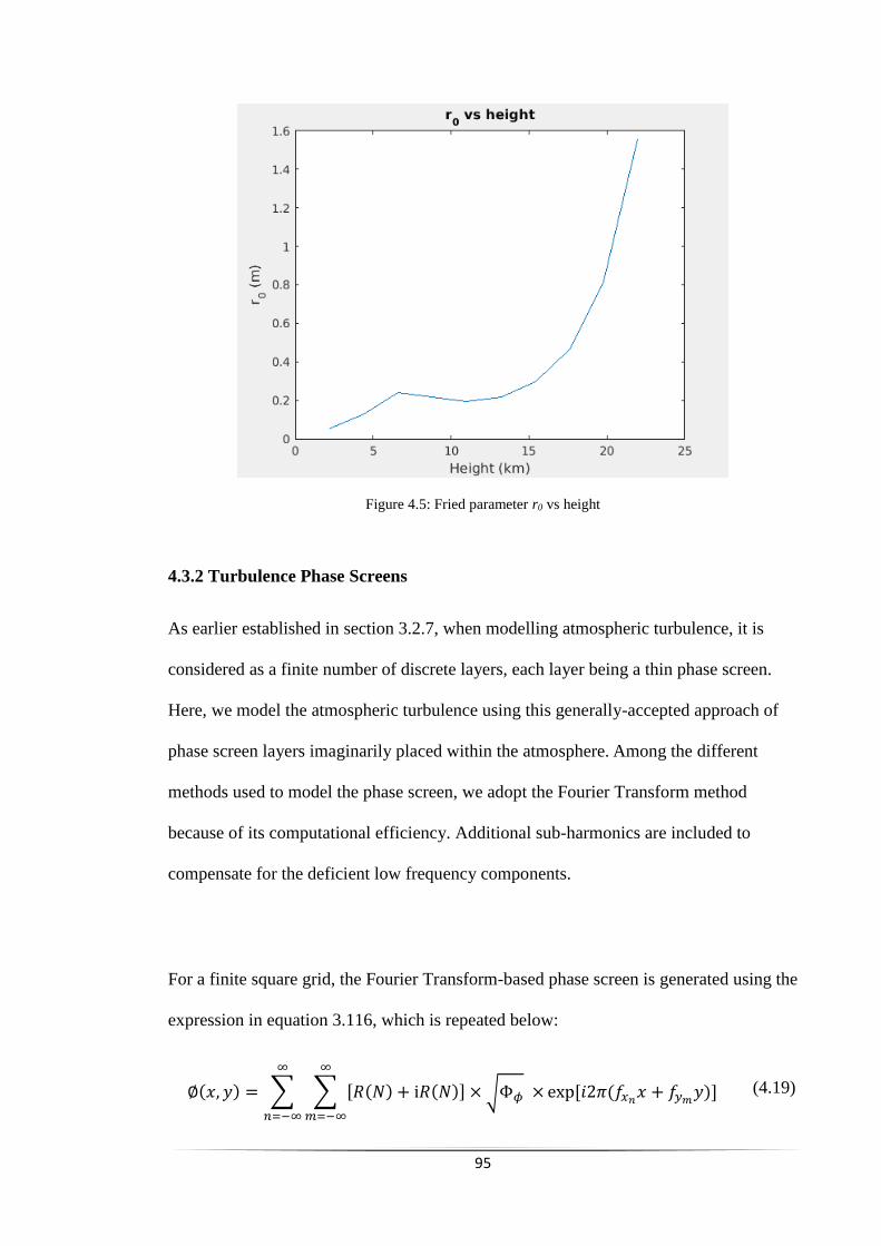
95
Figure 4.5: Fried parameter r0 vs height
4.3.2 Turbulence Phase Screens
As earlier established in section 3.2.7, when modelling atmospheric turbulence, it is
considered as a finite number of discrete layers, each layer being a thin phase screen.
Here, we model the atmospheric turbulence using this generally-accepted approach of
phase screen layers imaginarily placed within the atmosphere. Among the different
methods used to model the phase screen, we adopt the Fourier Transform method
because of its computational efficiency. Additional sub-harmonics are included to
compensate for the deficient low frequency components.
For a finite square grid, the Fourier Transform-based phase screen is generated using the
expression in equation 3.116, which is repeated below:
∅(𝑥, 𝑦) = ∑ ∑ [𝑅(𝑁) + i𝑅(𝑁)] × √Φ𝜙 ×
∞
𝑚=−∞
∞
𝑛=−∞
exp [𝑖2𝜋(𝑓𝑥𝑛𝑥 + 𝑓𝑦𝑚
𝑦)] (4.19)
96
where R represents Gaussian random numbers with zero mean and unit variance. N is
the number of grid points per side of the screen, 𝑓𝑥𝑛and 𝑓𝑦𝑚
are the discrete spatial
frequencies in the x and y directions. The 𝛷𝜙 is the phase Power Spectral Density (PSD)
of turbulence. For this, we use the modified von Karman’s phase PSD earlier defined in
equation 3.93 but repeated below, since it is the simplest that includes the inner and
outer scale:
Φ∅𝑚𝑣𝑘 = 0.49𝑟0
−5/3exp (−𝑘2/𝑘𝑚
2)
(𝑘2 + 𝑘02)11/6
(4.20)
The r0 is an implementation of equation 4.18 in terms of the Cn2. At this point, a fixed
Cn2 for all the phase screens is used to model the atmosphere for cases where the beam
is propagated across a horizontal and terrestrial path. But for the vertical and ground-to-
space propagation path, the Cn2 will be gradually-weakening with height in line with
equation 4.17. After generating the phase screens using equation 4.19, the deficient low
frequency components are generated based on the earlier defined equation 3.117,
repeated below:
∅𝑙𝑓(𝑥, 𝑦) = ∑ ∑ ∑ 𝐶𝑛,𝑚exp [𝑖2𝜋(𝑓𝑥𝑛𝑥 + 𝑓𝑦𝑚
𝑦)]
1
𝑚=−1
1
𝑛=−1
𝑁𝑝
𝑝=1
(4.21)
where n and m are discrete frequencies and each p represents the different grids. The
𝐶𝑛,𝑚 are the random draws of the Fourier series coefficients.

97
One of the scenarios to be considered in chapter 5 is a ground-to-space scenario where
the beams are propagated from sea level through turbulence up to 22 km altitude. In this
case, the phase screens are produced every interval of 2.2 km such that 10 gradually
weakening phase screens span equally across the 22 km height of atmospheric
turbulence as seen pictured on figure 4.6. This is suited for the split-step propagation
which will be adopted for the beam propagation in Chapter 5.
Figure 4.6: Phase screens for altitudes (2.2km to 22km). Grid 2000x2000 pixels.
Unit of phase (colour scale) in radians.
The phase screens grid side length as well as the number of pixel points N is taken to be
the same as those for the source plane and the observation plane, which were chosen to
satisfy the sampling constraints.

98
4.4 Chapter Conclusions
In this chapter, we were able to model the two beams; Gaussian and Bessel beams,
which will be propagated in the chapters 5 and 6. We went on to derive some
expressions to define the minimum source aperture radius for both beams, with their
respective altitudes, to ensure that not more than 50% of the initial beam power is lost in
transit before it arrives at the receiver. These definitions confirm the fact that the longer
the distance of the FSO communication, the bigger the required size of the aperture of
the transmitter and receiver to minimise power losses.
The second section of the chapter focused on modelling the atmospheric turbulence
phase screens, using the Fourier transform method. We also arrived at a model for Cn2
with respect to height, and based on this we derived a maximum height of 22 km above
which the effect of turbulence will be negligible. This maximum height of 22 km will
be very useful in Chapters 6 when simulating the optical beam propagation for a
ground-to-space scenario as the turbulence phase screens will terminate at this altitude,
and beyond this altitude the beam will be assumed to be propagating through a vacuum
for the rest of the path. Based on the same Cn2 model we derived, we saw that the Cn
2
will be considered fixed when modelling beam propagation through a horizontal
terrestrial path (ground-to-ground applications) as will be seen in Chapter 5.

99
CHAPTER 5
100
5.0 SHORT RANGE BEAM PROPAGATION THROUGH TURBULENCE
In this chapter, the two beams generated in chapter 4 (Gaussian and Bessel beams) will
be propagated for a short range of 2 km, first terrestrially with the transmitter and
receiver at the same height of 100m above the ground, and then vertically- upwards
with the transmitter on ground and the receiver at a 2 km altitude. A split step
propagation method is called up here, where the total propagation distance is sectioned
into smaller and equal intervals for more accurate modelling. We begin the chapter with
consideration of the Fresnel Propagation sampling regimes then propagate the two
beams without turbulence in order to investigate the diffraction effect on the beams. The
horizontal path propagation through turbulence assumes that the Cn2 will be fixed over
the 2 km, while the vertically-upwards path assumes a gradually weakening Cn2. The
turbulence is modelled using phase screens described earlier in chapter 4. We compare
the two scenarios (the horizontal 2 km path versus the vertically-upwards 2 km path)
and see which one is better for short range FSO designs.
5.1 Fresnel Propagation Sampling Regimes (TF vs IF)
As seen in section 3.1.4.1, there are two approximations to the Rayleigh-Sommerfeld
diffraction theory: the Fresnel and Fraunhofer Diffraction. Beam propagators are
modelled based on these approximations. The Fresnel number criterion, 𝑁𝑓 =𝑤2
𝜆𝑧, is
generally used to determine when the Fresnel expression can be applied with minimal
loss of accuracy or when the Fraunhofer would be more suitable, w is the beam radius.
If Nf is far less than (<<) 1, for example up to 20 to 30 times less than 1, then the
observation plane is generally regarded to be in the Fraunhofer region. But if Nf is > 1,
or slightly less or equal to 1, then it is in the Fresnel zone, hence the Fresnel
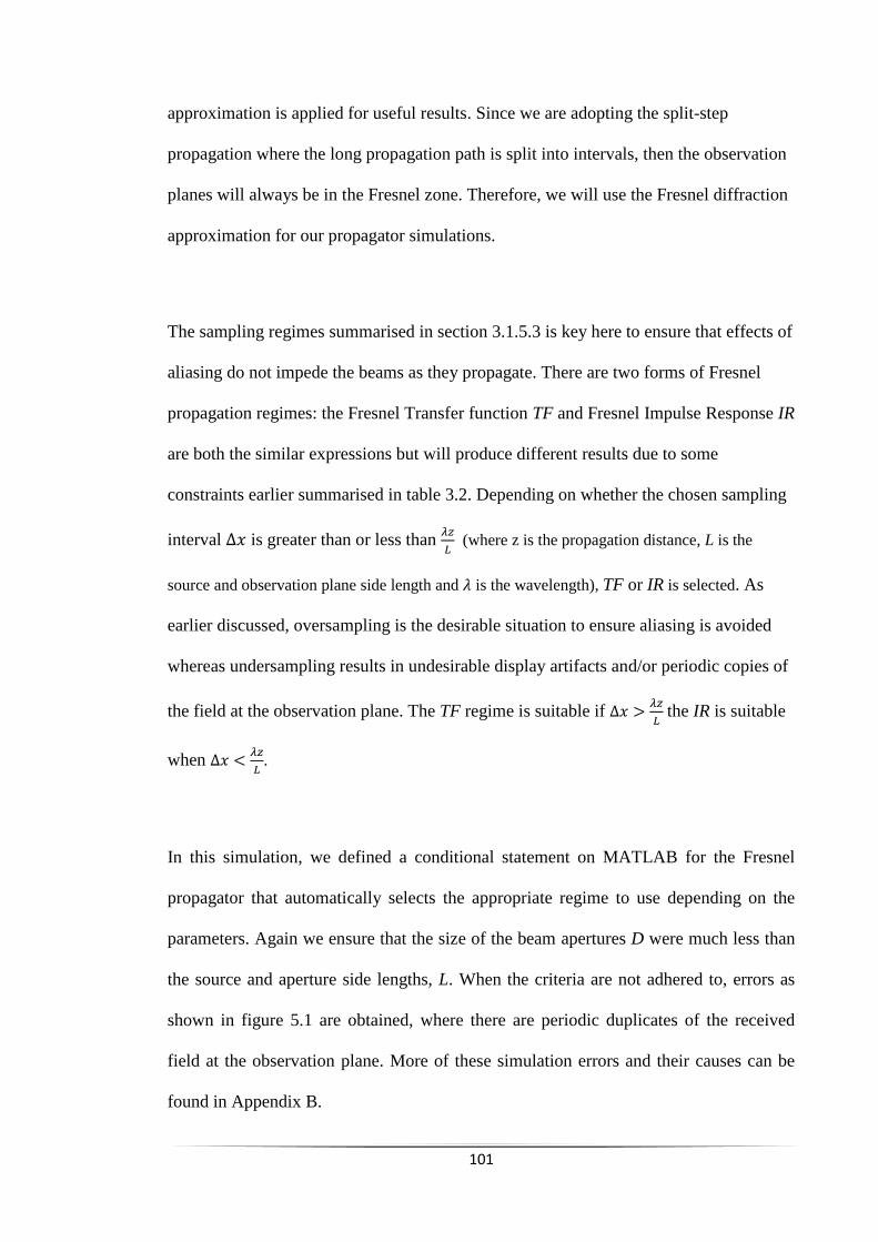
101
approximation is applied for useful results. Since we are adopting the split-step
propagation where the long propagation path is split into intervals, then the observation
planes will always be in the Fresnel zone. Therefore, we will use the Fresnel diffraction
approximation for our propagator simulations.
The sampling regimes summarised in section 3.1.5.3 is key here to ensure that effects of
aliasing do not impede the beams as they propagate. There are two forms of Fresnel
propagation regimes: the Fresnel Transfer function TF and Fresnel Impulse Response IR
are both the similar expressions but will produce different results due to some
constraints earlier summarised in table 3.2. Depending on whether the chosen sampling
interval ∆𝑥 is greater than or less than 𝜆𝑧
𝐿 (where z is the propagation distance, L is the
source and observation plane side length and 𝜆 is the wavelength), TF or IR is selected. As
earlier discussed, oversampling is the desirable situation to ensure aliasing is avoided
whereas undersampling results in undesirable display artifacts and/or periodic copies of
the field at the observation plane. The TF regime is suitable if ∆𝑥 >𝜆𝑧
𝐿 the IR is suitable
when ∆𝑥 <𝜆𝑧
𝐿.
In this simulation, we defined a conditional statement on MATLAB for the Fresnel
propagator that automatically selects the appropriate regime to use depending on the
parameters. Again we ensure that the size of the beam apertures D were much less than
the source and aperture side lengths, L. When the criteria are not adhered to, errors as
shown in figure 5.1 are obtained, where there are periodic duplicates of the received
field at the observation plane. More of these simulation errors and their causes can be
found in Appendix B.

102
Figure 5.1: Aliasing on propagated Gaussian beam
5.2 Beam Propagation without Turbulence
The lower atmosphere definitely contains a considerable amount of turbulence.
However, it is useful to monitor the effect of diffraction alone without turbulence, on
the Gaussian and Bessel beam as they propagate over a range. Both beams have been
apertured to the same radius of 0.2 m. Diffraction is known to cause the propagating
beam to spread resulting in the on axis intensity of the beam decaying as it diffracts
further.
The intensity error in figure 5.2 is the propagating beam intensity minus the intensity of
the initial beam (at ground level for vertical propagation), before propagation. Clearly,
the Gaussian beam diffracts a lot more than the Bessel beam as its intensity error from
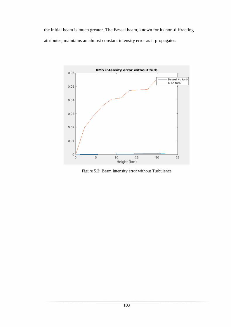
103
the initial beam is much greater. The Bessel beam, known for its non-diffracting
attributes, maintains an almost constant intensity error as it propagates.
Figure 5.2: Beam Intensity error without Turbulence

104
5.3 Beam Propagation through a fixed atmospheric Turbulence (for a 2 km
horizontal path)
For a ground-to-ground horizontal optical path, the strength of turbulence Cn2 across the
path will be fixed because the source and destination are at the same altitude. If the
transmitter and receiver are both at an elevation of 100 metres above sea level, the
corresponding strength of turbulence across the path Cn2 (100 m) from the Cn
2 (h) model
in equation 4.17 will be 1.64 × 10⁻¹⁵ m-2/3. Equation 4.17 is repeated below for easy
reference:
𝐶𝑛
2(ℎ) = 6.5 [3.593 × 10⁻³ (ℎ105⁄ )
10𝑒(−ℎ/1000) + 2.7 × 10⁻¹⁶𝑒(−ℎ/1500)] (5.1)
and the corresponding coherence parameter r0 is derived from equation 4.18, also
repeated below:
𝑟0,𝑝𝑤 = [0.423𝑘2 ∫ 𝐶𝑛2(ℎ)𝑑ℎ
ℎ
0
]
−3/5
(5.2)
We examine the propagation of the two beams across a 2 km horizontal path, through
the fixed turbulence Cn2 of 1.64 × 10⁻¹⁵ m-2/3, when both transmitter and receiver are at
100 m altitude. We use an inner scale l0 of 0.01 m and an outer scale L0 of 100 m. Again,
the two beams under consideration are apertured to 0.2 m radius. Fresnel diffraction is
used for the beam propagation and the split step propagation method is adopted,
splitting the 2 km path into 20 layers of 100 m each. The turbulence phase screens are
logically placed at each of the intervals. The wavelength 𝜆 = 500 nm, the array size
was 1024 × 1024 pixels2 representing an array of 8 × 8 m2.
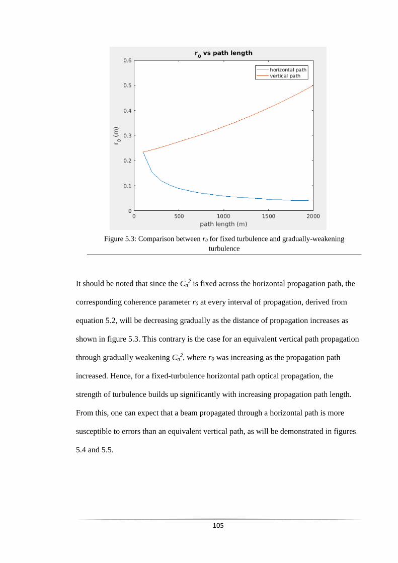
105
Figure 5.3: Comparison between r0 for fixed turbulence and gradually-weakening
turbulence
It should be noted that since the Cn2 is fixed across the horizontal propagation path, the
corresponding coherence parameter r0 at every interval of propagation, derived from
equation 5.2, will be decreasing gradually as the distance of propagation increases as
shown in figure 5.3. This contrary is the case for an equivalent vertical path propagation
through gradually weakening Cn2, where r0 was increasing as the propagation path
increased. Hence, for a fixed-turbulence horizontal path optical propagation, the
strength of turbulence builds up significantly with increasing propagation path length.
From this, one can expect that a beam propagated through a horizontal path is more
susceptible to errors than an equivalent vertical path, as will be demonstrated in figures
5.4 and 5.5.
106
Figure 5.4: RMS Intensity Error for beam propagation through fixed Turbulence.
The intensity error is defined as the intensity of the propagating beam minus the intensity of the
beam at sea level, before propagation.
When the two beams are propagated through the same 2 km horizontal ground-to-
ground path scenario described above, it can be seen in figure 5.4 that the Gaussian
beam is significantly aberrated by the strong turbulence as it propagates such that its
intensity error from the initial beam is rapidly increasing as it propagates. The Bessel
beam on the other hand, is only slightly aberrated as it propagates through the strong
turbulence and there is no much difference between its intensity error when it is
propagating through turbulence and when it is propagating without turbulence. As will
be seen in section 5.4, for an equivalent 2 km range but for a vertical upwards
propagation, the beams will experience less aberration as they propagate, compared to
the ground-to-ground horizontal range.
107
5.4 Beam Propagation through gradually-weakening atmospheric turbulence
In this scenario, the transmitter is assumed to be on the ground (at sea level) and the
propagation proceeds vertically-upwards to an altitude of 2 km. Again, Fresnel
diffraction is used for the beam propagation. The wavelength 𝜆 = 500 nm, the array
size was 1024 × 1024 pixels2 representing an array of 2 × 2 m2. The outer and lower
atmospheric scales used were 𝐿0 = 100 m and 𝑙0 = 0.01 m.
The same beam aperture radius Bw of 0.2 m is considered for both initial Gaussian and
Bessel beams, before propagating to the 2 km altitude. This allows us to be able to make
a sensible comparison with the horizontal propagation path scenario in section 5.3
which was also considered for the same 2 km range. The simulation of the atmospheric
turbulence for the vertically-upwards scenario is based on the model stated in equation
4.5 for a gradually diminishing Cn2 with height.
Figure 5.5 below illustrates the beams propagated in this scenario. Comparing figure 5.5
to figure 5.4, the Bessel beam still has a better performance than the Gaussian, as it was
in the horizontal ground-to-ground scenario. Furthermore, it can be observed that for the
same propagation range of 2 km, if the propagation path is horizontal (fixed turbulence),
the beams are more aberrated (with more intensity error) than for a vertical ground-to-
space path.

108
Figure 5.5: RMS Intensity Error for propagation through gradually-weakening turbulence. The
intensity error is defined as the intensity of the propagating beam minus the intensity of the
beam at sea level, before propagation.
5.5 Chapter Summary
In this chapter, we considered the propagation of the two beams for a 2 km FSO range.
The primary aim was to demonstrate that the orientation of the path (whether horizontal
or vertical) is an important consideration in FSO system design. The Gaussian beam
clearly was more susceptible to diffraction and turbulence in all the scenarios as it had a
higher Intensity error performance than the Bessel beam. Furthermore, the horizontal 2
km path, where both transmitter and receiver where 100 m above the ground, had a
poorer intensity error performance than the 2 km vertically-upwards path. This is
because the turbulence in the latter is gradually-weakening whereas that of the former is
fixed resulting in accumulation of the turbulence effects as it propagates. Hence, we
have shown that in the design of an FSO system, it is critical to ensure a considerable
difference in altitude between the transmitter and receiver, rather than placing them on
the same altitude. For example, the transmitter could be positioned on the ground level
while the receiver is positioned at the top of a sky-scrapper or a high mountain.

109
CHAPTER 6

110
6.0 LONG DISTANCE BEAM PROPAGATION THROUGH TURBULENCE
(UP TO 22 KM ALTITUDE AND DEEP SPACE)
This chapter will investigate the propagation of the two beams under consideration, the
Gaussian and Bessel beams, from ground to space. The transmitter is assumed to be at
sea level propagating vertically upwards. The first section will investigate the beams
propagated up to the 22 km height; this height which was earlier derived in Chapter 4 to
be the assumed maximum height for the existence of atmospheric turbulence. The
second section will analyse what happens when the beams are propagated beyond the 22
km height, in vacuo, up to an altitude of 100 km. The performance of the two beams are
compared to each other as they propagate through these two scenarios. We also
investigated the performance of different beam sizes, for the two beams, in order to
select the beam size that is more suitable for the different performance criteria.
The useful propagation targets and distances earlier derived in tables 4.1 and 4.2 are
brought forward here in table 6.1, this time including labels to help identify their
respective beam radii as they will be useful subsequently.
Table 6.1: Useful propagation targets and their respective half power beam radii
Label Target Altitude (km) 𝒘𝟎.𝟓𝑷 𝑩𝒘𝒎𝒊𝒏
∘ An A320 Aircraft ceiling 12 59mm 44mm
+ Higher Altitude Aircrafts 27 89mm 77mm
∗ International Space Station (ISS) 340 315mm 235mm
× Low Earth Orbit (LEO) Satellite 700 452mm 337mm
□ Global Position System (GPS) Satellite 20,350 2.44m 1.82m
◊ Geostationary Orbit (GEO) Satellite 35786 3.23m 2.41m
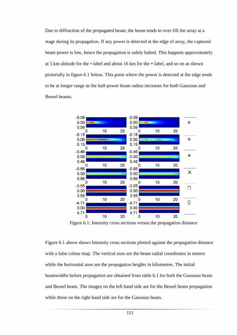
111
Due to diffraction of the propagated beam, the beam tends to over-fill the array at a
stage during its propagation. If any power is detected at the edge of array, the captured
beam power is low, hence the propagation is safely halted. This happens approximately
at 5 km altitude for the ∘ label and about 16 km for the + label, and so on as shown
pictorially in figure 6.1 below. This point where the power is detected at the edge tends
to be at longer range as the half-power beam radius increases for both Gaussian and
Bessel beams.
Figure 6.1: Intensity cross sections versus the propagation distance
Figure 6.1 above shows Intensity cross sections plotted against the propagation distance
with a false colour map. The vertical axes are the beam radial coordinates in meters
while the horizontal axes are the propagation heights in kilometres. The initial
beamwidths before propagation are obtained from table 6.1 for both the Gaussian beam
and Bessel beam. The images on the left hand side are for the Bessel beam propagation
while those on the right hand side are for the Gaussian beam.
112
6.1 Beam Propagation from Ground to 22 km altitude
In this section, the two beams will be propagating from ground to space through
atmospheric turbulence up to the turbulence altitude limit of 22 km. The results that will
be discussed henceforth are obtained after averaging over 100 runs of the simulation.
An ideal and desirable FSO communication system needs to have the following
attributes:
The transmitting beam needs to have a high peak intensity with as little of the
beam power as possible contained in the sidelobes.
As much of the initial beam power as possible, successfully delivered to the
receiver.
The peak of the transmitting beam intensity profile needs to remain around the
propagation axis. This will enable it not to wander away from the receiver
aperture.
The transmitter optics (including the receiver) should be as small as possible for
convenience.
The remainder of this section discusses to what extent the above attributes have been
realised when comparing the propagation of the different beamwidths of the Gaussian
and the Bessel beam. This will considered based on 4 different performance measure:
Normalised captured power, Peak Position error, RMS Intensity error and Beam
Wander.
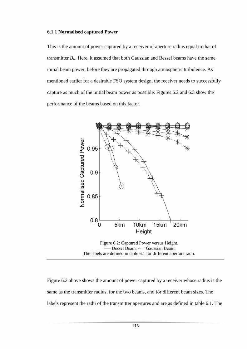
113
6.1.1 Normalised captured Power
This is the amount of power captured by a receiver of aperture radius equal to that of
transmitter Bw. Here, it assumed that both Gaussian and Bessel beams have the same
initial beam power, before they are propagated through atmospheric turbulence. As
mentioned earlier for a desirable FSO system design, the receiver needs to successfully
capture as much of the initial beam power as possible. Figures 6.2 and 6.3 show the
performance of the beams based on this factor.
Figure 6.2: Captured Power versus Height.
—– Bessel Beam. ∙∙∙∙∙∙ Gaussian Beam.
The labels are defined in table 6.1 for different aperture radii.
Figure 6.2 above shows the amount of power captured by a receiver whose radius is the
same as the transmitter radius, for the two beams, and for different beam sizes. The
labels represent the radii of the transmitter apertures and are as defined in table 6.1. The
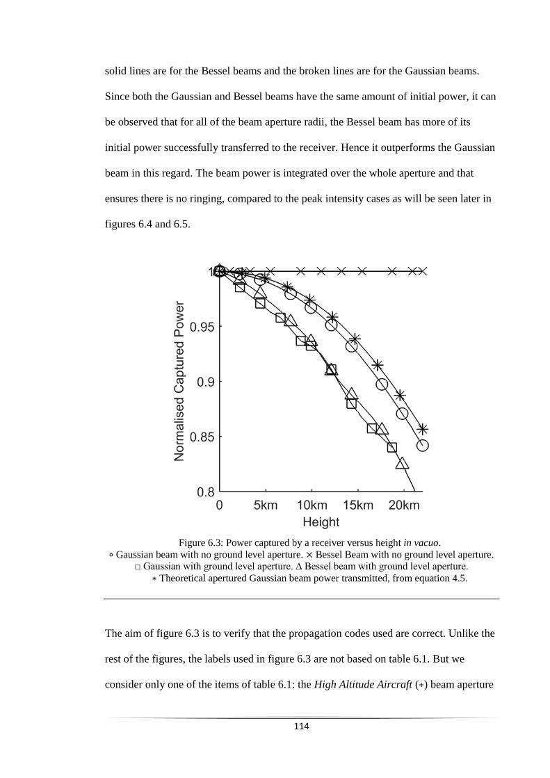
114
solid lines are for the Bessel beams and the broken lines are for the Gaussian beams.
Since both the Gaussian and Bessel beams have the same amount of initial power, it can
be observed that for all of the beam aperture radii, the Bessel beam has more of its
initial power successfully transferred to the receiver. Hence it outperforms the Gaussian
beam in this regard. The beam power is integrated over the whole aperture and that
ensures there is no ringing, compared to the peak intensity cases as will be seen later in
figures 6.4 and 6.5.
Figure 6.3: Power captured by a receiver versus height in vacuo. ∘ Gaussian beam with no ground level aperture. × Bessel Beam with no ground level aperture.
□ Gaussian with ground level aperture. ∆ Bessel beam with ground level aperture.
∗ Theoretical apertured Gaussian beam power transmitted, from equation 4.5.
The aim of figure 6.3 is to verify that the propagation codes used are correct. Unlike the
rest of the figures, the labels used in figure 6.3 are not based on table 6.1. But we
consider only one of the items of table 6.1: the High Altitude Aircraft (+) beam aperture
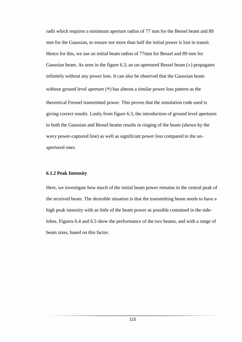
115
radii which requires a minimum aperture radius of 77 mm for the Bessel beam and 89
mm for the Gaussian, to ensure not more than half the initial power is lost in transit.
Hence for this, we use an initial beam radius of 77mm for Bessel and 89 mm for
Gaussian beam. As seen in the figure 6.3, an un-apertured Bessel beam (×) propagates
infinitely without any power loss. It can also be observed that the Gaussian beam
without ground level aperture (∘) has almost a similar power loss pattern as the
theoretical Fresnel transmitted power. This proves that the simulation code used is
giving correct results. Lastly from figure 6.3, the introduction of ground level apertures
to both the Gaussian and Bessel beams results in ringing of the beam (shown by the
wavy power-captured line) as well as significant power loss compared to the un-
apertured ones.
6.1.2 Peak Intensity
Here, we investigate how much of the initial beam power remains in the central peak of
the received beam. The desirable situation is that the transmitting beam needs to have a
high peak intensity with as little of the beam power as possible contained in the side-
lobes. Figures 6.4 and 6.5 show the performance of the two beams, and with a range of
beam sizes, based on this factor.
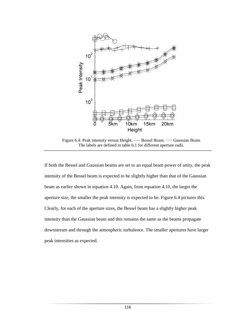
116
Figure 6.4: Peak intensity versus Height. —– Bessel Beam. ∙∙∙∙∙∙ Gaussian Beam
The labels are defined in table 6.1 for different aperture radii.
If both the Bessel and Gaussian beams are set to an equal beam power of unity, the peak
intensity of the Bessel beam is expected to be slightly higher than that of the Gaussian
beam as earlier shown in equation 4.10. Again, from equation 4.10, the larger the
aperture size, the smaller the peak intensity is expected to be. Figure 6.4 pictures this.
Clearly, for each of the aperture sizes, the Bessel beam has a slightly higher peak
intensity than the Gaussian beam and this remains the same as the beams propagate
downstream and through the atmospheric turbulence. The smaller apertures have larger
peak intensities as expected.
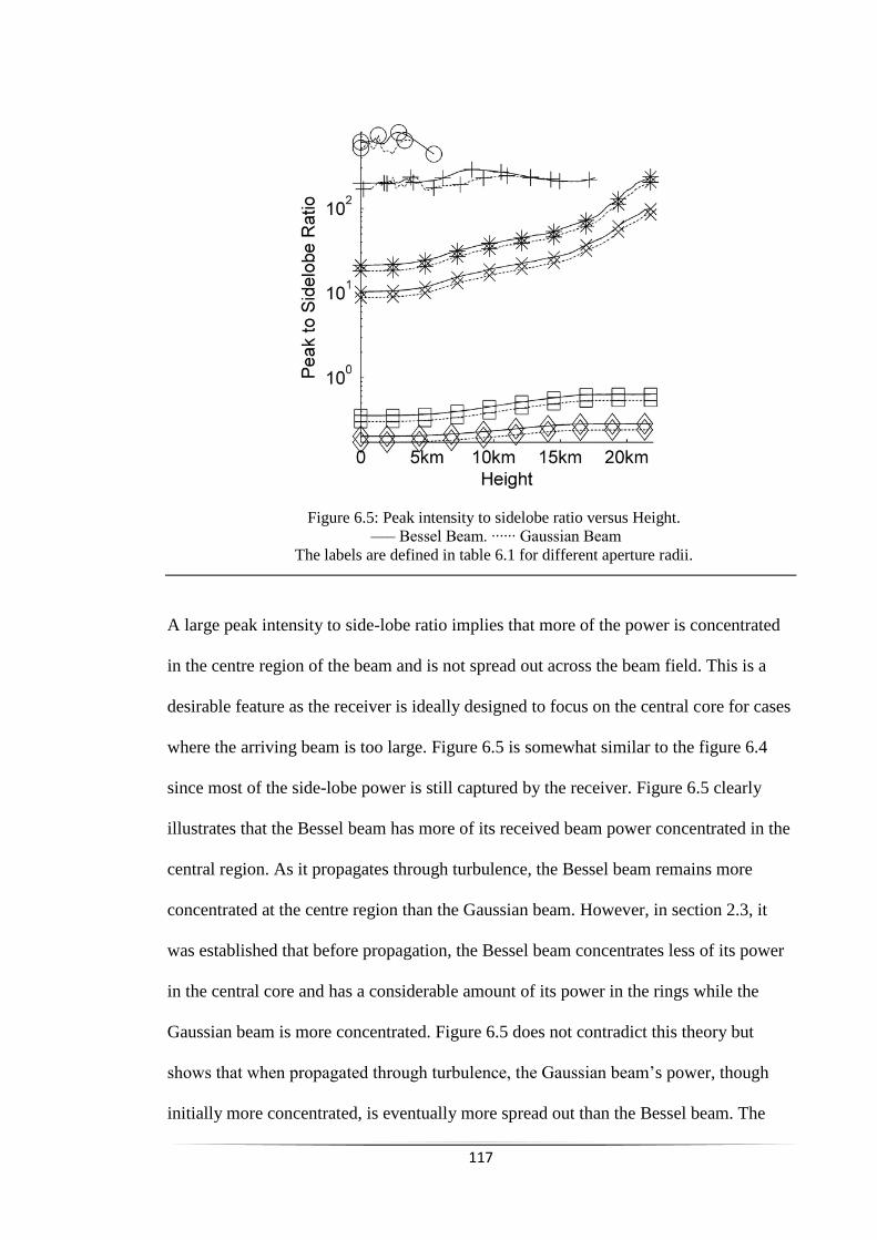
117
Figure 6.5: Peak intensity to sidelobe ratio versus Height.
—– Bessel Beam. ∙∙∙∙∙∙ Gaussian Beam
The labels are defined in table 6.1 for different aperture radii.
A large peak intensity to side-lobe ratio implies that more of the power is concentrated
in the centre region of the beam and is not spread out across the beam field. This is a
desirable feature as the receiver is ideally designed to focus on the central core for cases
where the arriving beam is too large. Figure 6.5 is somewhat similar to the figure 6.4
since most of the side-lobe power is still captured by the receiver. Figure 6.5 clearly
illustrates that the Bessel beam has more of its received beam power concentrated in the
central region. As it propagates through turbulence, the Bessel beam remains more
concentrated at the centre region than the Gaussian beam. However, in section 2.3, it
was established that before propagation, the Bessel beam concentrates less of its power
in the central core and has a considerable amount of its power in the rings while the
Gaussian beam is more concentrated. Figure 6.5 does not contradict this theory but
shows that when propagated through turbulence, the Gaussian beam’s power, though
initially more concentrated, is eventually more spread out than the Bessel beam. The

118
effect of the ringing at the edge of the aperture is seen in the slight wavy plot lines but
this is minimal because the peak intensity position can be anywhere within the aperture,
not necessarily at the centroid position.
6.1.3 Intensity Error
Here, we measure the performance of the beams based on the RMS value of the
difference between the intensity of the propagating beam (through turbulence) and that
of the initial beam before it was propagated (at sea level in this case with z = 0). The
performance of the beams based on this criterion is illustrated in figure 6.6. However, in
figure 6.7, we have a special case were the intensity error is the difference between the
propagating beam intensity and the intensity of the unaberrated beam that has travelled
the same distance but without turbulence.
Figure 6.6: RMS Intensity Error versus Height. The intensity error is the intensity of the
propagating beam minus the intensity of the beam before propagation.
—– Bessel Beam. ∙∙∙∙∙∙ Gaussian Beam
The labels are defined in table 6.1 for different aperture radii.
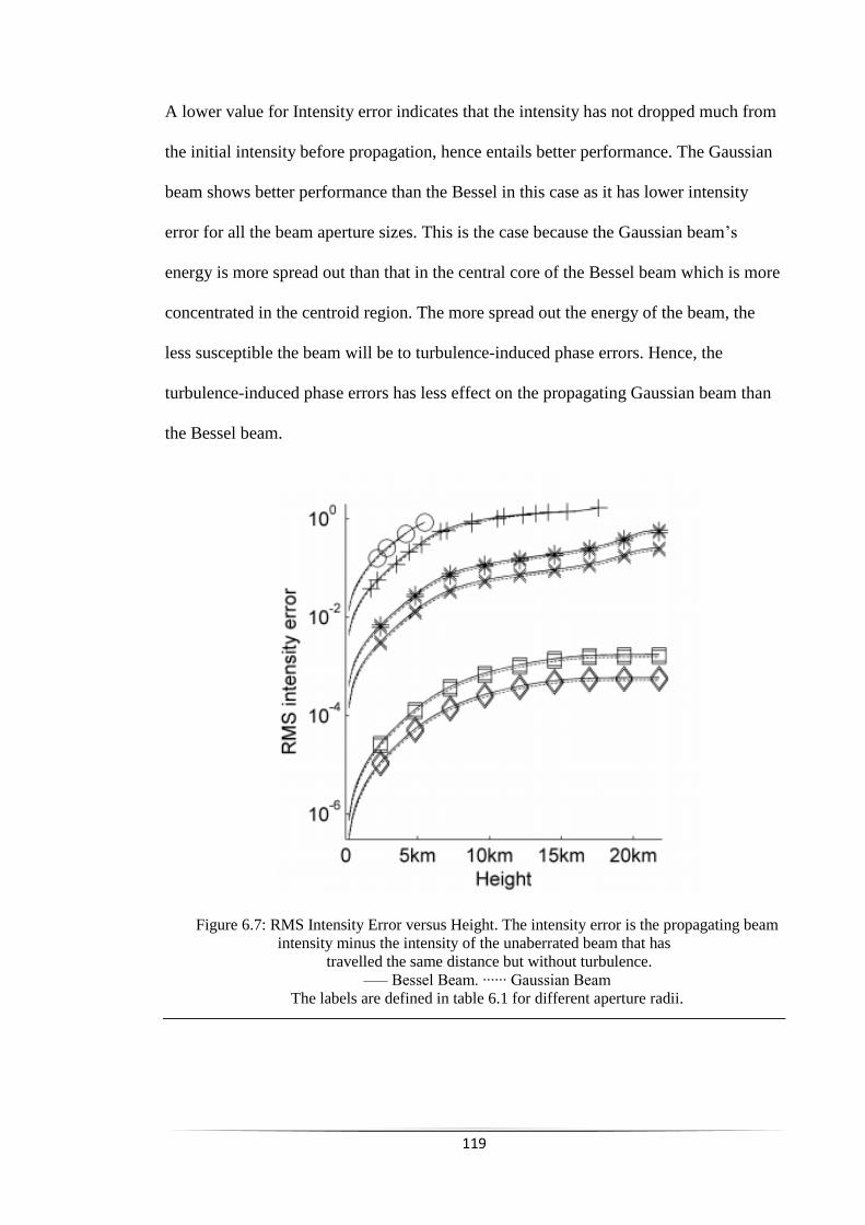
119
A lower value for Intensity error indicates that the intensity has not dropped much from
the initial intensity before propagation, hence entails better performance. The Gaussian
beam shows better performance than the Bessel in this case as it has lower intensity
error for all the beam aperture sizes. This is the case because the Gaussian beam’s
energy is more spread out than that in the central core of the Bessel beam which is more
concentrated in the centroid region. The more spread out the energy of the beam, the
less susceptible the beam will be to turbulence-induced phase errors. Hence, the
turbulence-induced phase errors has less effect on the propagating Gaussian beam than
the Bessel beam.
Figure 6.7: RMS Intensity Error versus Height. The intensity error is the propagating beam
intensity minus the intensity of the unaberrated beam that has
travelled the same distance but without turbulence.
—– Bessel Beam. ∙∙∙∙∙∙ Gaussian Beam
The labels are defined in table 6.1 for different aperture radii.

120
Figure 6.7 shows the Intensity error from a different light. The Intensity error here is the
difference between the beam intensity as it propagates through atmospheric turbulence
and the beam intensity when it is propagating in vacuo. Again here, the Gaussian has a
slightly better performance than the Bessel beam, hence the Bessel beam is more
affected by turbulence than the Gaussian beam. For both figures 6.6 and 6.7, the larger
beam apertures have better performance with less intensity errors as the beam power is
directly proportional to beam size in line with equations 4.2 and 4.10.
6.1.4 Peak Position Error
This is known as Beam wander – the drift of the propagating beam’s peak intensity
position from the initial centroid position of the beam as a result of phase errors from
the atmospheric turbulence. The initial beams are both created such that the pixel
position of the peak intensity is in the centroid position of the source grid.
Figure 6.8: Peak position error ratio versus Height.
—– Bessel Beam. ∙∙∙∙∙∙ Gaussian Beam
The labels are defined in table 6.1 for different aperture radii.

121
The peak position error on the y-axis of figure 6.8 is defined as the propagating beam’s
peak position minus the initial peak position of the beam before propagation (that is at z
= 0). Here we see that both Bessel and Gaussian beams have identical beam wander
results since they are both propagating through the same turbulence. The Bessel beams
self-healing attribute cannot save it from the phase error as a result of propagating
through atmospheric turbulence. Clearly from figure 6.8, the beam wander becomes
more severe as the beams propagate further down the path, through atmospheric
turbulence. Figure 6.9 illustrates this and supports these points from a different
perspective, it plots the y-axis centroid positions of the beams, where the initial centroid
position in this case is at the 512-pixel position.
Figure 6.9: Centroid position versus Height.
—– Bessel Beam. - - - Gaussian Beam
The labels are defined in table 6.1 for different aperture radii.
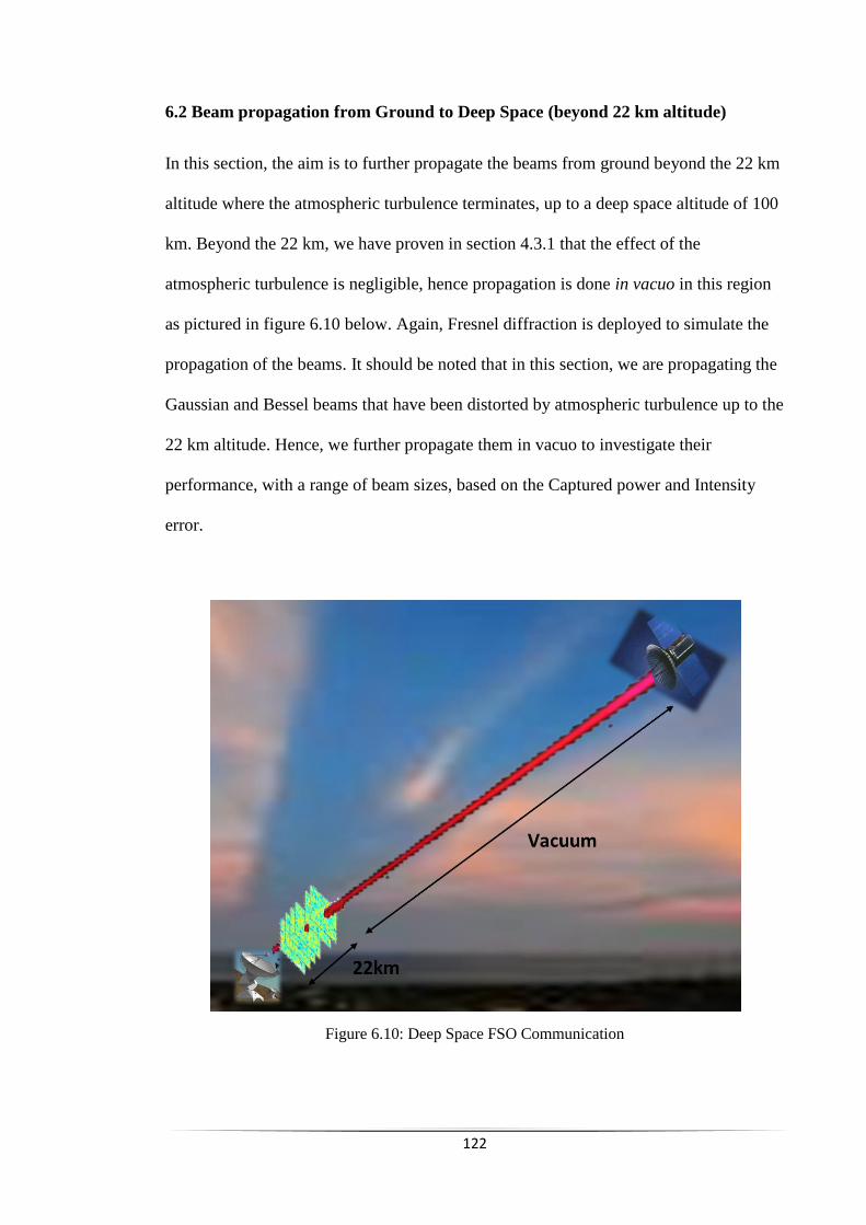
122
6.2 Beam propagation from Ground to Deep Space (beyond 22 km altitude)
In this section, the aim is to further propagate the beams from ground beyond the 22 km
altitude where the atmospheric turbulence terminates, up to a deep space altitude of 100
km. Beyond the 22 km, we have proven in section 4.3.1 that the effect of the
atmospheric turbulence is negligible, hence propagation is done in vacuo in this region
as pictured in figure 6.10 below. Again, Fresnel diffraction is deployed to simulate the
propagation of the beams. It should be noted that in this section, we are propagating the
Gaussian and Bessel beams that have been distorted by atmospheric turbulence up to the
22 km altitude. Hence, we further propagate them in vacuo to investigate their
performance, with a range of beam sizes, based on the Captured power and Intensity
error.
Figure 6.10: Deep Space FSO Communication
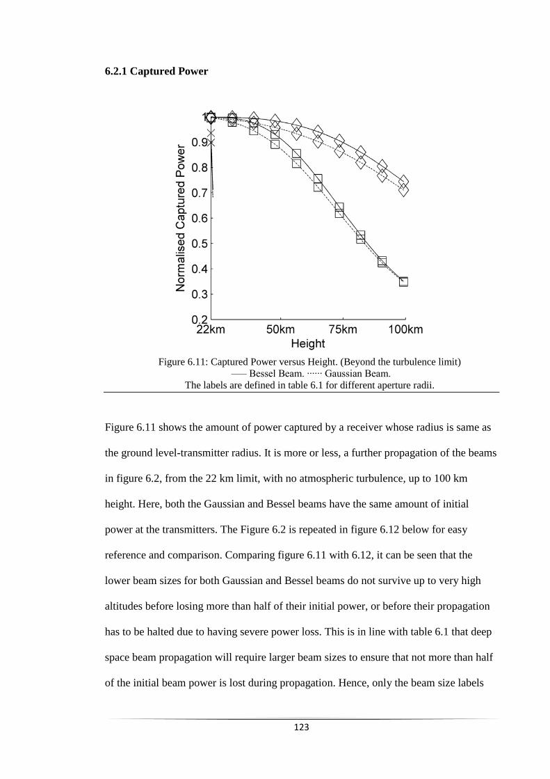
123
6.2.1 Captured Power
Figure 6.11: Captured Power versus Height. (Beyond the turbulence limit)
—– Bessel Beam. ∙∙∙∙∙∙ Gaussian Beam.
The labels are defined in table 6.1 for different aperture radii.
Figure 6.11 shows the amount of power captured by a receiver whose radius is same as
the ground level-transmitter radius. It is more or less, a further propagation of the beams
in figure 6.2, from the 22 km limit, with no atmospheric turbulence, up to 100 km
height. Here, both the Gaussian and Bessel beams have the same amount of initial
power at the transmitters. The Figure 6.2 is repeated in figure 6.12 below for easy
reference and comparison. Comparing figure 6.11 with 6.12, it can be seen that the
lower beam sizes for both Gaussian and Bessel beams do not survive up to very high
altitudes before losing more than half of their initial power, or before their propagation
has to be halted due to having severe power loss. This is in line with table 6.1 that deep
space beam propagation will require larger beam sizes to ensure that not more than half
of the initial beam power is lost during propagation. Hence, only the beam size labels

124
for □ GPS satellite and ◊ GEO satellite are able to propagate beyond the 22 km height.
Figure 6.11 also shows that beyond the turbulence limit, the beams still get diffracted as
they propagate, hence the captured power still gradually diminishes with height. The
Bessel beam still maintains the advantage of having more of its initial beam power
successfully captured by the receiver, compared to the Gaussian beam. Because of the
absence of atmospheric turbulence in this region, the captured power declines at a
slower rate than it does in the atmospheric turbulence region (below the 22 km).
Figure 6.12: Captured Power versus Height. (Within the turbulence limit)
—– Bessel Beam. ∙∙∙∙∙∙ Gaussian Beam.
The labels are defined in table 6.1 for different aperture radii.
125
6.2.2 Intensity Error
The intensity error performance of the both beams beyond the atmosphere is going to be
similar to the one shown in figure 5.2 when the beams were propagated without
turbulence: the Bessel beam has better Intensity error performance than the Gaussian
beam. This is contrary to the case in the turbulence region from ground level to 22 km
height, where the Gaussian beam had a better intensity error performance as shown in
figure 6.7. Recall that we had established in section 6.1.3 that the reason the Gaussian
beam had a better Intensity error performance than the Bessel beam, when propagating
through atmospheric turbulence, was the Gaussian beam energy is more spread out
hence will be less prone to be turbulence-induced errors, compared to the Bessel beam
central core whose energy is more concentrated.
However, in this case where the beams have gone beyond the turbulence and now
propagating in the absence of the turbulence, there will be no more phase errors on the
beams. Hence, the more energy-concentrating Bessel beam now has a better Intensity
error performance than the more spread-out Gaussian beam. Another reason the Bessel
beam will eventually have a better Intensity error performance in this region is its self-
healing property. This property enables it to eventually recover its inward diffraction
attribute, after being distorted by atmospheric turbulence and the due to the inward
diffraction, its on-axis intensity remains almost invariant as it propagates in this no-
turbulence region. The Gaussian beam, on the other hand, does not possess this self-
healing attribute and continues to diffract as it propagates in this region. This implies
that the Bessel beam, though initially slightly under-performing in the turbulence region,
eventually has better Intensity error than the Gaussian beam when propagated beyond
the turbulence limit to deep space platforms.

126
6.3 Chapter Summary
This chapter investigated the propagation of the Gaussian and Bessel beams vertically
upwards to high space orbits of 22 km altitude and beyond, up to 100 km. With the
transmitter at ground level, we first considered the propagation of the beams up to the
atmospheric turbulent limit of 22 km. Here, we analysed the performances of the two
beams compared them to each other based on the defined performance criteria. We saw
that the Bessel beam majorly outperformed the Gaussian based on the Captured power
and Peak intensity while the Gaussian beam had better performance based on Intensity
error. The both beams had a similar Beam wander performance since they are
propagating through the same atmosphere. The second section of the chapter considered
the ground to Deep Space scenario, where the beams are further propagated beyond the
22 km turbulence limit in vacuo. With no atmospheric turbulence, the beams were only
subjected to diffraction showing that their performances decayed at a slower rate with
distance. The Bessel beam had most of the advantage compared to the Gaussian beam
as it had better Captured power and recovered its inward-diffracting attributes to
produce better Intensity error performance.

127
CHAPTER 7

128
7.0 CONCLUSION AND RECOMMENDATION
7.1 Conclusion
Free Space Optics (FSO) clearly have huge potential including secure and robust high
capacity communication links. The more common Gaussian beam is known to be
extremely susceptible to diffraction resulting in the spread of its energy and lowering
the amount that reaches the receiver. Since the main impairments to FSO have been
identified to be Diffraction and Atmospheric turbulence, the so-called non-diffracting
self-healing Bessel beam is an attractive alternative.
We have confirmed that the non-diffracting attribute of the Bessel beam is only for the
ideal case where the beam will have to possess an infinite radius. But to produce the
beam in reality, the beam will have to be approximated with the radius truncated into an
aperture function and this will limit the range over which the Bessel beam remains non-
diffracting to Zmax.
Furthermore, we have shown that the longer the distance of the FSO communication,
the bigger the size of the transmitter and receiver apertures required to minimise power
losses. This applies for both Gaussian and Bessel beams. This solution will be costly
and bring an additional inconvenience of size and weight of the transmitter and receiver.
To ensure that at least half of the initial power of the beam is delivered to the receiver,
the Bessel beam will have a smaller transmitter and receiver aperture size requirements
compared to the Gaussian beam, if both beams had an equal initial power before
propagation.

129
When both beams were propagated through atmospheric turbulence, we were able to
compare the effect of fixed turbulence in a horizontal 2 km path to that of a gradually-
weakening turbulence in a vertically-upwards 2 km path. In the horizontal path scenario,
both the transmitter and receiver are at the same altitude, and 2 km apart while the
vertically-upwards scenario assumed that the transmitter was at sea level while the
receiver was at 2 km altitude. We have seen that beams propagated in the vertically-
upwards scenario are less aberrated because the turbulence in this case is gradually
weakening with height, compared to the horizontal path fixed turbulence case where the
turbulence keeps building up. From this, it is clear that in the design of an FSO system,
it is more effective to ensure a substantial altitude difference between the transmitter
and receiver to minimise the effect of atmospheric turbulence. For instance, the
transmitter could be on the ground level while the receiver is positioned at the top of a
sky-scrapper or a high mountain.
For the ground – to – space atmospheric turbulence scenario, we have arrived at a
maximum altitude of 22 km above which atmospheric turbulence will be negligible.
This 22 km altitude was obtained from an approximate model we derived from a variant
of the Hufnagel-Andrews-Philips model of Cn2 with respect to height, with a few more
assumptions. Above this 22 km altitude, it is therefore assumed that the beams would be
propagating in a vacuum. Hence, we propagated both the Bessel and Gaussian beam
through a ground –to – space turbulence terminating at the 22 km. Then we investigated
the performance of the two beams using four categories of performance measure namely:
Beam wander, captured power, Intensity error and Peak intensity. The Bessel beam
proved to have better performance based on the captured power and peak intensity. The
130
beam wander effect on both beams appeared to be identical. The Gaussian beam, on the
other hand, slightly outperformed the Bessel beam based on the RMS Intensity error.
Beyond the 22 km turbulence limit, both beams were propagated in vacuo. As expected,
both beams still diffract as they propagate in vacuo. The Bessel beam still maintains a
better Captured-power performance compared to the Gaussian as it has more of its
initial power captured at the receiver at a height of 100 km. Only large beam sizes are
able to travel that far without more than half their initial beam lost in transit. Because of
the absence of atmospheric turbulence in this region, the captured power declines at a
slower rate than it does in the turbulence region. Unlike the turbulence region, the
Bessel beam now demonstrates a better Intensity-error performance than the Gaussian
as it possesses inward diffraction properties will aid its peak intensity to be almost
invariant as it propagates. This indicates that the Bessel beam, though initially slightly
under-performing in turbulence, eventually has better Intensity error than the Gaussian
beam when propagated beyond the turbulence limit to deep space platforms.
In order to ensure that the advantages that the Bessel beam has over the Gaussian are
sustained, the Bessel beam needs to be produced from high efficiency lasers. This could
be challenging in reality, especially if the produced beam has to travel for a long
distance. Another condition, to ensure that the Bessel beam retains its advantage is that
it has to be produced with no side-lobes (rings); this implies that the radial frequency
should be chosen such that the beam aperture is equal to the first root of the Bessel
function. As shown in this research, the ring-less Bessel beams travels for a
considerable distance through turbulence also ensuring efficient power delivery to the
receiver, and especially since the turbulence distorts the ring structure of the beam as it

131
propagates. However, many lasers available in the market inherently produce beams
with a near-Gaussian profile. Due to being more readily available, the Gaussian beam
could be more frequently utilised and compensated for its poor power delivery
performance by having higher transmitted beam power.
Finally, it is widely proposed that earth stations for Ground –to-Space communications
be located on mountain tops. Clearly, situating an earth station on a mountain as high as
Kilimanjaro for instance, of about 5.8 km height, will ensure that the most of the strong
turbulence is avoided as the turbulence weakens with height.
7.2 Future Work
Diffraction and atmospheric turbulence are the most popular impairments to Free Space
Optical Communications. These two phenomena and their respective effects on the
Gaussian and Bessel beams have been exhaustively covered and analysed in this work.
However, there exists another impairment to FSO – Aerosol Scattering. The additional
effect of Aerosol Scattering to Free Space Optical Communications would make our
model more accurate. Aerosols are tiny solid particles and liquid droplets present in the
earth’s atmosphere, below the planetary boundary layer. They tend to drift from the
stratosphere downwards towards the earth surface. Aerosols vary greatly in size
(generally from 0.002 to 100 microns), chemical composition, source, and distribution
in time and space. Common examples of aerosols in the atmosphere are smoke, fog,
smog, dust and cloud cover. The presence of these aerosols does affect (absorb or
scatter) sun light or any other optical signal propagating through the atmosphere. The
effect of an aerosol on light depends on:

132
i. Colour of the aerosol particle: Bright coloured/ translucent particles reflect
significant amount of light in all directions while dark aerosols can absorb
significant amount of lights.
ii. The constituent of the aerosol: Pure sulphates as well as nitrates reflect a
significant amount of light incident on them. Black carbon, on the other hand,
tends to absorb more radiation. Dust particles have varying effects on incident
light depending on composition. Salt particles tend to reflect all light they
encounter.
iii. The shape of the aerosol particle: Atmospheric aerosols are generally spherical
but cylindrical particles could be found in viruses and asbestos fibres.
iv. Size of the aerosol particle:
This is usually considered with respect to the wavelength of the incident beam.
In Aerosol Optics, the necessary equations for scattered field were derived based on a
factor that assumes that the beam size of the incident beam is laterally infinite. This
assumption is ideal as an infinite beam size cannot be realistically produced in the
laboratory. However, it is a logical assumption since the incident beam will completely
drown the aerosol particle as the beam size is very large compared to the size of the
aerosol particle. Hence the Scattering and Absorption will be independent of the
incident beam size.
There are two main scattering theories widely used to approximate the scattering by a
single sphere namely the Mie Scattering and Rayleigh scattering. Rayleigh scattering is
known to apply in scenarios where the size of the aerosol particle is much less than the
133
wavelength of the incident light. For example solar radiations scattered by atmospheric
gases. Unlike the Rayleigh scattering, the conditions for applying Mie scattering is
somewhat arbitrary based on the size of the particle with respect to the wavelength of
the incident light. However, past research has generally defined Mie Scattering as being
applied for scenarios where the particle size is comparable or greater than the
wavelength of the incident light. Mie Scattering is specific to aerosols and cloud
particles which are generally spherical in shape.
For the proposed work of incorporating aerosol scattering into our propagation model,
we will be considering atmospheric aerosols which are known to be spherical in shape
with size comparable or greater than the incident optical wavelength. Considering the
shape and size of the atmospheric particles, the so called Mie’s scattering theory is most
suitable. However, the Mie’s theory only considers scattering by a single particle
whereas natural environments like the atmosphere have a collection of particles. Past
research on light scattering by a collection of particles mainly focuses on cylindrical
particles, not spherical. Hence we seek to model the propagation of Gaussian and Bessel
beams through a collection of spherical atmospheric particles present in the lower
atmosphere up to the atmospheric boundary layer 1.5 km altitude. The proposed model
will investigate the additional effect of aerosol scattering on the two beams.
Expressions will be derived for Amplitude Scattering Matrix for the scattering of optical
beams from a collection of arbitrarily-placed spherical atmospheric particles. We will
assume a forward scattering situation with no back scattering. Light absorption by the
aerosol particles will be neglected while we focus on only scattering from the particles.
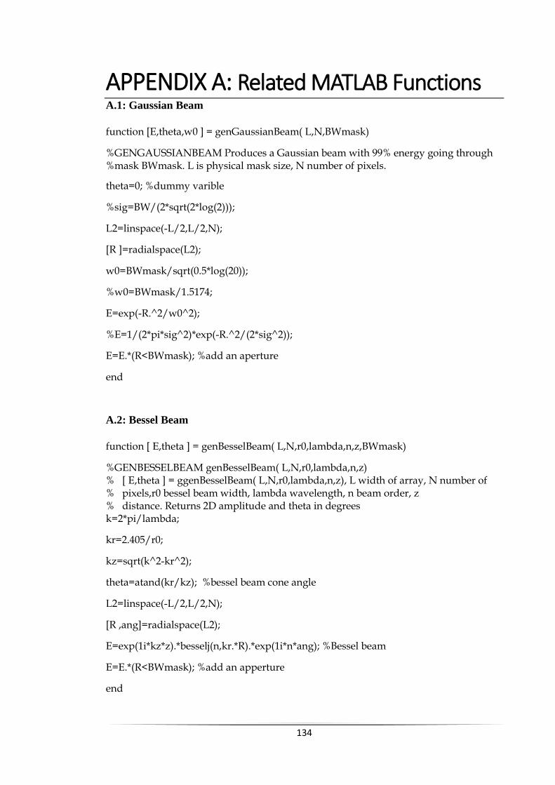
134
APPENDIX A: Related MATLAB Functions A.1: Gaussian Beam
function [E,theta,w0 ] = genGaussianBeam( L,N,BWmask)
%GENGAUSSIANBEAM Produces a Gaussian beam with 99% energy going through %mask BWmask. L is physical mask size, N number of pixels.
theta=0; %dummy varible
%sig=BW/(2*sqrt(2*log(2)));
L2=linspace(-L/2,L/2,N);
[R ]=radialspace(L2);
w0=BWmask/sqrt(0.5*log(20));
%w0=BWmask/1.5174;
E=exp(-R.^2/w0^2);
%E=1/(2*pi*sig^2)*exp(-R.^2/(2*sig^2));
E=E.*(R<BWmask); %add an aperture
end
A.2: Bessel Beam
function [ E,theta ] = genBesselBeam( L,N,r0,lambda,n,z,BWmask)
%GENBESSELBEAM genBesselBeam( L,N,r0,lambda,n,z) % [ E,theta ] = ggenBesselBeam( L,N,r0,lambda,n,z), L width of array, N number of % pixels,r0 bessel beam width, lambda wavelength, n beam order, z % distance. Returns 2D amplitude and theta in degrees k=2*pi/lambda;
kr=2.405/r0;
kz=sqrt(k^2-kr^2);
theta=atand(kr/kz); %bessel beam cone angle
L2=linspace(-L/2,L/2,N);
[R ,ang]=radialspace(L2);
E=exp(1i*kz*z).*besselj(n,kr.*R).*exp(1i*n*ang); %Bessel beam
E=E.*(R<BWmask); %add an apperture
end

135
A.4: Fresnel Propagation
function [ u2, L2] = FresnelPropagation( u1,L,lambda,z, varargin )
%FRESNELPROPAGATION Propergates using Fresenel diffraction % [ u2, L2] = FresnelPropagation( u1,L,lambda,z, [method, [options..] ) % propagates complex field u1 by distance z. Lambda is the wavelength, % L is the width of the array in physical units. Note the array must be % square. The function works out which propagation method to use by % default. This can be overridden by setting method to 'auto', or a function handle'propTF', % 'propIR' or 'propFT'. See those individual help files for details. % options are 'nowarn' - suppress warnings, 'verbose' increase verbose output. % The function returns u2 the complex field at z, and L2 the x coordinates. % Philip Birch 2013 Copyright
warn=1;
verbose=0;
if(length(varargin)>1)
for p=2:length(varargin)
switch varargin{p}
case 'nowarn'
warn=0;
case 'verbose'
verbose=1;
end
end
end
[n ,m]=size(u1);
if(n~=m)
error('PMB:FresnelSq','Input field must be square');
end
N=FresnelNumber(L,lambda,z);
if(N>1 && warn)
warning('PMB:Fresprop','The Fresnel number, %f, is greater than one. Results maybe
inaccurate',N);
end
dx=L/n;
if dx>=lambda*z/L
%use TF
prophandle=@propTF;
else
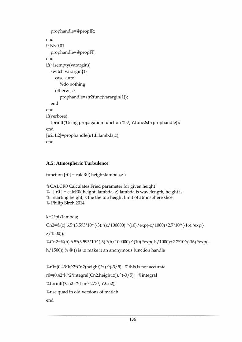
136
prophandle=@propIR;
end
if N<0.01
prophandle=@propFF;
end
if(~isempty(varargin))
switch varargin{1}
case 'auto'
%do nothing
otherwise
prophandle=str2func(varargin{1});
end
end
if(verbose)
fprintf('Using propagation function %s\n',func2str(prophandle));
end
[u2, L2]=prophandle(u1,L,lambda,z);
end
A.5: Atmospheric Turbulence
function [r0] = calcR0( height,lambda,z )
%CALCR0 Calculates Fried parameter for given height % [ r0 ] = calcR0( height ,lambda, z) lambda is wavelength, height is % starting height, z the the top height limit of atmosphere slice. % Philip Birch 2014
k=2*pi/lambda;
Cn2=@(z) 6.5*(3.593*10^(-3).*(z/100000).^(10).*exp(-z/1000)+2.7*10^(-16).*exp(-
z/1500));
%Cn2=@(h) 6.5*(3.593*10^(-3).*(h/100000).^(10).*exp(-h/1000)+2.7*10^(-16).*exp(-
h/1500));% @ () is to make it an anonymous function handle
%r0=(0.43*k^2*Cn2(height)*z).^(-3/5); %this is not accurate
r0=(0.42*k^2*integral(Cn2,height,z)).^(-3/5); %integral
%fprintf('Cn2=%f m^-2/3\n',Cn2);
%use quad in old versions of matlab
end
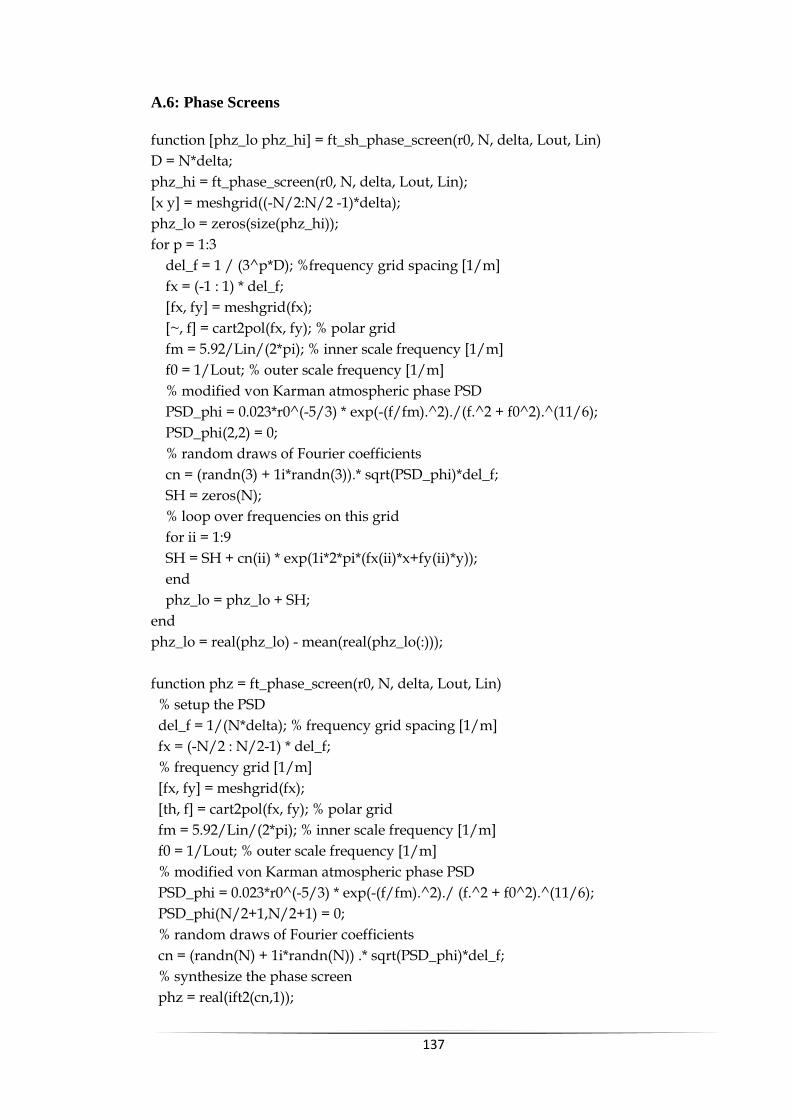
137
A.6: Phase Screens
function [phz_lo phz_hi] = ft_sh_phase_screen(r0, N, delta, Lout, Lin)
D = N*delta;
phz_hi = ft_phase_screen(r0, N, delta, Lout, Lin);
[x y] = meshgrid((-N/2:N/2 -1)*delta);
phz_lo = zeros(size(phz_hi));
for p = 1:3
del_f = 1 / (3^p*D); %frequency grid spacing [1/m]
fx = (-1 : 1) * del_f;
[fx, fy] = meshgrid(fx);
[~, f] = cart2pol(fx, fy); % polar grid
fm = 5.92/Lin/(2*pi); % inner scale frequency [1/m]
f0 = 1/Lout; % outer scale frequency [1/m]
% modified von Karman atmospheric phase PSD
PSD_phi = 0.023*r0^(-5/3) * exp(-(f/fm).^2)./(f.^2 + f0^2).^(11/6);
PSD_phi(2,2) = 0;
% random draws of Fourier coefficients
cn = (randn(3) + 1i*randn(3)).* sqrt(PSD_phi)*del_f;
SH = zeros(N);
% loop over frequencies on this grid
for ii = 1:9
SH = SH + cn(ii) * exp(1i*2*pi*(fx(ii)*x+fy(ii)*y));
end
phz_lo = phz_lo + SH;
end
phz_lo = real(phz_lo) - mean(real(phz_lo(:)));
function phz = ft_phase_screen(r0, N, delta, Lout, Lin)
% setup the PSD
del_f = 1/(N*delta); % frequency grid spacing [1/m]
fx = (-N/2 : N/2-1) * del_f;
% frequency grid [1/m]
[fx, fy] = meshgrid(fx);
[th, f] = cart2pol(fx, fy); % polar grid
fm = 5.92/Lin/(2*pi); % inner scale frequency [1/m]
f0 = 1/Lout; % outer scale frequency [1/m]
% modified von Karman atmospheric phase PSD
PSD_phi = 0.023*r0^(-5/3) * exp(-(f/fm).^2)./ (f.^2 + f0^2).^(11/6);
PSD_phi(N/2+1,N/2+1) = 0;
% random draws of Fourier coefficients
cn = (randn(N) + 1i*randn(N)) .* sqrt(PSD_phi)*del_f;
% synthesize the phase screen
phz = real(ift2(cn,1));

138
end
function g = ift2(G, delta_f)
% function g = ift2(G, delta_f)+.
N = size(G, 1);
g = ifftshift(ifft2(ifftshift(G))) * (N * delta_f)^2;
end
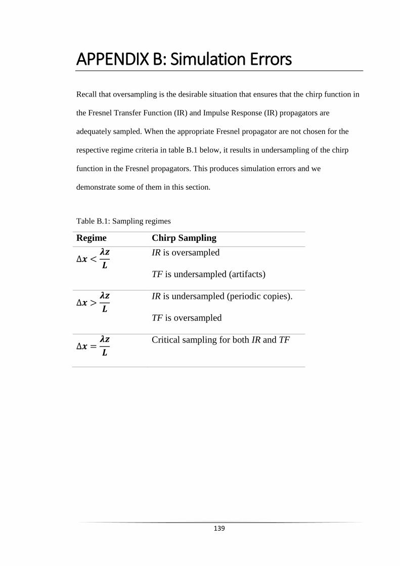
139
APPENDIX B: Simulation Errors
Recall that oversampling is the desirable situation that ensures that the chirp function in
the Fresnel Transfer Function (IR) and Impulse Response (IR) propagators are
adequately sampled. When the appropriate Fresnel propagator are not chosen for the
respective regime criteria in table B.1 below, it results in undersampling of the chirp
function in the Fresnel propagators. This produces simulation errors and we
demonstrate some of them in this section.
Table B.1: Sampling regimes
Regime Chirp Sampling
∆𝒙 <𝝀𝒛
𝑳
IR is oversampled
TF is undersampled (artifacts)
∆𝒙 >𝝀𝒛
𝑳
IR is undersampled (periodic copies).
TF is oversampled
∆𝒙 =𝝀𝒛
𝑳
Critical sampling for both IR and TF
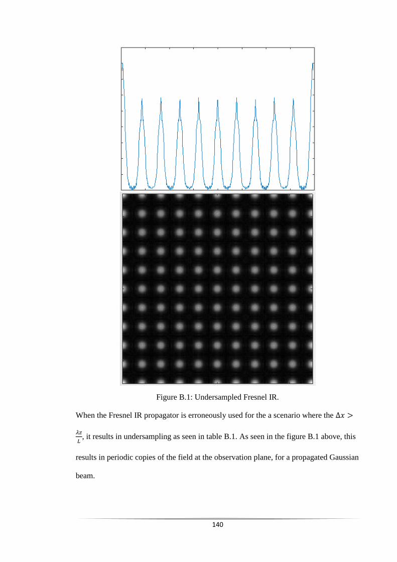
140
Figure B.1: Undersampled Fresnel IR.
When the Fresnel IR propagator is erroneously used for the a scenario where the ∆𝑥 >
𝜆𝑧
𝐿, it results in undersampling as seen in table B.1. As seen in the figure B.1 above, this
results in periodic copies of the field at the observation plane, for a propagated Gaussian
beam.
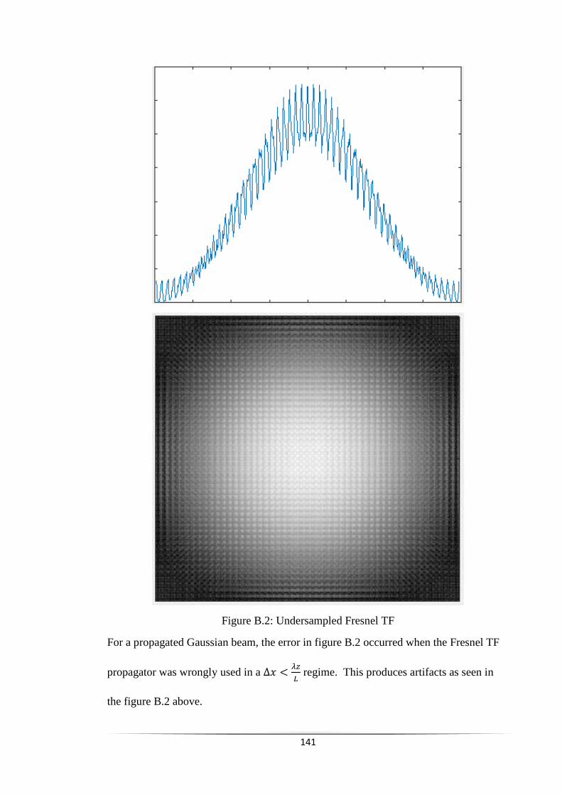
141
Figure B.2: Undersampled Fresnel TF
For a propagated Gaussian beam, the error in figure B.2 occurred when the Fresnel TF
propagator was wrongly used in a ∆𝑥 <𝜆𝑧
𝐿 regime. This produces artifacts as seen in
the figure B.2 above.

142
Figure B.3: Artifacts at the edge of the array
If the beam is not limited to a guard area or aperture with diameter D ≪ the source grid
length L, it results in artifacts at the edge of the observation grid array due to periodic
extension properties of FFT.
143
REFERENCES
1. Stamatious V. Kartalopoulos, Free Space Optical Networks for Ultra-Broad Band
Services, 1st ed., IEEE, John Wiley & Sons, Inc. (2011), pp 1 – 10.
2. Deva K. Borah et al, “A Review of communication-oriented Optical Wireless
Systems.” EURASIP Journal on Wireless Communications and Networking (2012).
3. B. A. Witvliet et al, Comparison of UHF Measurement with the propagation model
of Recommendation ITU-R P.156, Radiocommunications Agency Netherlands, 2010.
pg. 13.
4. Stamatious V. Kartalopoulos, Free Space Optical Networks for Ultra-Broad Band
Services, 1st ed., IEEE, John Wiley & Sons, Inc. (2011), Chapter 1.
5. Suriza Ahmad Zabidi et al, “The Effect of Weather on Free Space Optics
Communication Under Tropical Weather Conditions and a Proposed Setup for
Measurement.” ICCCE (2010).
6. M. S. Awan et al. “Transmission of High Data Rate Optical Signals in Fog and Snow
Conditions.” IEEE Wireless VITAE (2009).
7. P.W. Kruse , L. McGlauchlin, and O.H. Vaughan , Elements of Infrared Technology:
Generation, Transmission and Detection, John Wiley & Sons, New York (1962).
8. E. Leitgeb et al. “The Influence of Dense Fog on Optical Wireless Systems, analysed
by Measurements in Graz for Improving the Link-Reliability.” ICTON (2006).
9. J. Durnin, “Exact solutions for nondiffracting beams. I. The Scalar theory,” J. Opt.
Soc. Am. A, 4 (1987), pp. 651-654.
10. J. Durnin, J.J. Miceli and J.H. Eberly, Phys. Rev. Lett., 66 (1991), pp. 838.
11. D. McGloin and K. Dholakia, “Bessel beams: Diffraction in a new light,”
Contemporary Physics, 46 (2005), pp. 15-28.
12. W. Nelson, J. P. Palastro, C.C. Davis and P. Spangle, “Propagation of Bessel and
Airy Beams through Atmospheric Turbulence”. J. Opt. Soc. Am. A, Vol. 31, No 3,
2014.
13. P. Sprangle and B. Hafizi, “Comment on nondiffractive beams,” Phys. Rev. Lett. 66,
1991, pg. 837.
14. L.C. Andrews, R. Phillips, R. Crabbs, D. Wayne, T. Leclerc, and P. Sauer,
“Atmospheric Channel Characterisation for ORCA Testing at NTTR,” Proc. Of
SPIE Vol. 7588 (2010).
144
15. Sergio Martelluci and Massimo Santarsiero (ed.,), “Free and Guided Optical Beams,”
Proc. Int. Sch. Quant. Electronics, Erice Slcily (2002).
16. Orazio Svelto, Principles of Lasers, 5th ed. (Springer London, 2010), pp. 150 – 158.
17. Anthony Siegman, Lasers (University Science Books, California, 1986), Chapter 17.
18. Paul F. Goldsmith, Quasioptical Systems: Gaussian Beam Quasioptical
Propagation and Applications (Wiley-IEEE Press, 1997), Chapter 2.
19. Robert K. Tyson, Principles of Adaptive Optics (Academic Press, London, 1991),
pp. 1- 23.
20. B. D. Guenther, Modern Optics, 1st ed. (Oxford University Press, 1990), pp. 356-
364.
21. H. Kogelnik and T. Li, “Laser Beam and Resonator”, Appl. Opt. 5, 10, (1966),
pp.1550-1567.
22. Stamatious V. Kartalopoulos, Free Space Optical Networks for Ultra-Broad Band
Services, 1st ed. (IEEE, John Wiley & Sons, 2011), Chapter 1.
23. Rudiger Paschotta, Encyclopedia of Laser Physics and Technology, volume 1, (John
Wiley & Sons, 2008).
24. H. Weber, “High Average Power Solid State Lasers for Material Processing and
Fiber Transmission,” in Laser Applications for Mechanical Industry, S. Martelluci
et al (ed.), Series E: Applied Sciences, 238, (Springer Science + Business,
Dordrecht, 1993), pg. 13.
25. Amnon Yariv, Quantum Electronics, 3rd ed. (John Wiley & Sons, New York, 1989),
Chapter 3 and 7.
26. L. Allen et al, “Orbital Angular momentum of light and the transformation of
Laguerre-Gaussian laser modes”, Phys. Rev. A 45, 11 (1992).
27. M. Bandres and J. Gutierrez-Vega, “Ince-Gaussian beams,” Opt. Lett. 29, 2 (2004),
pp. 144-146.
28. E. Karimi et al, “Hypergeometric-Gaussian modes”, Opt. Lett. 32, 21 (2007), pp.
3053- 3055.
29. J. Durnin, J.J. Miceli and J.H. Eberly, “Comparison of Bessel and Gaussian beams,”
Opt. Lett., 13 (1988), pp. 79-80.
30. G Indebetouw, “Non-diffracting Optical Fields: some remarks on their Analysis and
Synthesis,” J. Opt. Soc. Am. A., 6, 1 (1989), pp. 150 – 152.
31. Mohamed Mahmoud et al, “Propagation of Bessel beam generated using finite-

145
width Durnin ring,” Appl. Opt. 52, 2 (2013), pp. 256-263.
32. S Fujiwara. “Optical properties of conical surfaces. 1. Reflecting cones,” J. Opt. Soc.
Am., 52 (1962), pp. 287-292.
33. Angela Dudley et al, “Unravelling Bessel Beams,” OSA Optics & Photonics News,
24, 6 (2013), pp. 22-29.
34. J. Durnin, J.J. Miceli and J.H. Eberly, “Diffraction-Free Beams,” Phys. Rev. Lett.,
58 (1987), pp. 1499-1501.
35. C. A. McQueen, J. Arlt and K. Dholakia, “An experiment to study ‘nondiffracting’
light beam,” Am. J. Phys., 67 (1999), pp. 912-915.
36. Islam Abdo et al, “Effects of ring width on ring generated Bessel beam,” Proc SPIE,
8236 (2012).
37. N. Chattrapiban et al, “Generation of non-diffracting beams by use of Spatial Light
Modulator,” Opt. Lett., 28 (2003), pp. 2183-2185.
38. J. Turunen, A. Vasara and A. Friberg, “Holographic generation of diffraction-free
Beams,” Appl. Opt. 27, 19 (1988), pp. 3959 – 3962.
39. A. Vasara, J. Turunen, and A. Friberg, ”Realization of general nondiffracting beams
with computer-generated holographs,” J. Opt. Soc. Am. A., 6, 11 (1989), pp. 1748 –
1754.
40. C. Paterson and R. Smith, “Higher-order Bessel waves produced by Axicon-type
Computer-generated holograms,” Optical Communications 124 (1996), pp. 599-602
41. S. H. Tao, X. C. Yuan and B. Ahluwalia, “The generation of an array of
nondiffracting beams by a single composite computer generated hologram,” J. of
Optics A: Pure and Applied Optics, 7 (2005), pp. 40-46.
42. E. M. Epperlein (ed.,), “Experimental Investigation of Bessel-Beam Characteristics,”
LLE Review, 46 (January-March 1991), Section 2A.
43. S. Chavez-Cerda et al, “Holographic generation and Orbital angular momentum of
Higher-order Mathieu beams,” J. Opt. B: Quantum Semiclass. Opt., 4 (2002), S52-
S57.
44. Robert Nowack, “A tale of two beams: An elementary Overview of Gaussian beams
and Bessel Beams”, Stud. Geophys. Geod., 56 (2012), pp. 355 – 372.
45. Jason D. Schmidt, Numerical Simulation of Optical Wave Propagation, with
examples in MATLAB, SPIE Press Bellingham, Chapter 1.
46. J Jackson, Classical Electrodynamics, 3rd ed., John Wiley and Sons Inc., (1998).
146
47. Andrew Zangwill, Modern Electrodynamics, Cambridge University Press (2013), pp.
44-45.
48. J. W. Goodman, Introduction to Fourier Optics, 2nd Ed., McGraw-Hill Companies
Inc, 1996.
49. R. Bracewell, Two Dimensional Imaging, Prentice-Hall, New Jersey (1994).
50. David Voelz, “Computational Fourier Optics, a Matlab tutorial,” SPIE Press,
Bellingham (2011), pp. 1-27.
51. E. Brigham, The Fast Fourier Transform and its Applications, Prentice-Hall, New
Jersey (1988).
52. David Voelz, “Computational Fourier Optics, a Matlab tutorial,” SPIE Press,
Bellingham (2011), pp. 47-86.
53. A Sommerfeld, Optics, vol. IV, of Lectures on Theoretical Physics, Academic Press,
New York (1954).
54. Francesco Grimaldi, Bologna, Italy: Vittorio Bonati (1665), pp. 1-11. (In Latin).
55. Eugene Hecht, Optics, 3rd ed., Addison Wesley Longman Inc. (1998), Chapter 10.
56. Christiaan Huygens, Treatise on Light, Dover Publication, New York (1962).
57. Augustin Fresnel, “ Memoir on the Diffraction of Light”, in The Wave Theory of
Light-Memoirs by Huygens, Young and Fresnel, American Book Company (1819),
pp. 79-145.
58. Gustav Kirchhoff, “Zur Theorie der Lichtstrahlen”, Weidemann Ann., 2, 28 (1883),
pg. 663.
59. Jason D. Schmidt, Numerical Simulation of Optical Wave Propagation, with
examples in MATLAB, SPIE Press Bellingham, Chapter 6.
60. W. Coles, J. Filice, R. Frehlich, and M. Yadlowsky, “Simulation of Wave
propagation in three-dimensional random media,” Appl. Opt. 34, 12 (1995), pp.
2089-2101.
61. N. Delen and B. Hooker, “Verification and comparison of a fast Fourier transform-
based full diffraction method for tilted and offset planes,” Appl. Opt. 40, 21 (2001),
pp. 3525-3531.
62. S. Coy, “Choosing Mesh spacing and mesh dimensions for wave optics simulation,”
Proc. SPIE 5894 (2005).
63. J. Mansell, R. Praus and S. Coy, “Determining Wave-Optics mesh parameters for
complex Optical systems,” Proc SPIE 6675 (2007).
147
64. L. Onural, “Some mathematical properties of the uniformly sampled Quadratic
phase Function and associated issues in Digital Fresnel Diffraction simulations,”
Opt. Eng. 43, 11 (2004), pp. 2557-2563.
65. P. Roberts, “A Wave Optics propagation code,” Tech. Rep. TR-760, the Optical
Sciences Company (1986).
66. G. A. Tyler and D. L. Fried, “A wave optics propagation Algorithm,” Tech. Rep.
TR-451, the Optical Sciences Company (1982).
67. D. Voelz and M Roggemann, “Digital simulation of Scalar Optical diffraction:
revisiting Chirp function Sampling criteria and Consequences,” Appl. Opt. 48, 32
(2009), pp. 6132 – 6142.
68. C. Rydberg and J. Bengtsson, “Efficient Numerical representation of the Optical
field for the propagation of partially coherent radiation with a specified spatial and
temporal Coherent function,” J. Opt. Soc. Am. A. 23, 7 (2006), pp. 1616-1625."
69. Jason D. Schmidt, Numerical Simulation of Optical Wave Propagation, with
examples in MATLAB, SPIE Press Bellingham, Chapter 7.
70. David Voelz, “Computational Fourier Optics, a Matlab tutorial,” SPIE Press,
Bellingham (2011), pp. 191-198.
71. Jason D. Schmidt, Numerical Simulation of Optical Wave Propagation, with
examples in MATLAB, SPIE Press Bellingham, Chapter 9.
72. Robert K. Tyson, Principles of Adaptive Optics, Academic Press Limited San Diego
(1991), pp. 25 – 50.
73. A. N. Kolmogorov, “The local structure of turbulence in an incompressible viscous
Fluids for very large Reynolds numbers,” C. R. (Doki) Acad. Sci. U.S.S.R. 30 (1941),
pp.301-305.
74. Javier Jimenez, “The Contributions of A. N. Kolmogorov to the Theory of
Turbulence”, Arbor Magazine CLXXVIII, 704, Agosto (2004), pp 589-606.
75. A. D. Wheelon, Electromagnetic Scintillation: Volume 2, Weak Scattering,
Cambridge University Press (2003).
76. G. K Batchelor, The Theory of Homogeneous Turbulence, Cambridge University
Press, London (1953).
77. A. Kolmogorov, in Turbulence; Classic Papers on Statistical Theory, S. K.
Friedlander and L.Topper, eds., Interscience Publishers (1961), pp. 151 -157.
78. Stanley Corrsin, Journal of Applied Physics, Volume 22 (1951), pp. 469 – 473.

148
79. V. I. Tartaskii, Wave Propagation in a Turbulent Medium, Translated by R. A.
Silverman McGraw Hill, New York (1961).
80. J. W. Strohbehn, ed., Laser Beam Propagation in the Atmosphere, Springer-Verlag,
New York (1978), pp. 9 - 43.
81. V. I. Tartaskii, The Effect of the Turbulent Atmosphere on Wave Propagation, U. S.
Dept. of Commerce, National Information Technical Service, Springfield VA
(1971).
82. V. Tatarskii, Wave Propagation in a turbulent medium, McGraw Hill, New York
(1961).
83. L.C. Andrews and R. L. Philips, Laser Beam Propagation Through Random Media,
2nd ed., SPIE Press, Bellingham, WA (2005).
84. Arnold Tunick et al, “Characterisation of optical Turbulence (Cn2) data measured at
ARLA_LOT facility,” ARL-MR-625, US Army Research Laboratory, Adelphi, MD
20783-1145 (2005).
85. E. A. Murphy, E.M. Dewan, and S.M Sheldon, “Daytime comparisons of Cn2
models to measurements in a desert location”. SPIE, 551(1985), pp. 156-162.
86. R. R. Beland, “Propagation through atmospheric optical turbulence,” in the Infrared
and ElectroOptical Systems Handbook, F. G. Smith, ed., vol. 2, SPIE Opt. Eng.
Press, Bellingham (1993), Chapter 2.
87. A. Belmonte, “Feasibility Study for the simulation of beam propagation:
Consideration of coherent Lidar performance,” Appl. Opt., 39 (2000), pp. 5426-
5445.
88. R. E. Hufnagel, “Propagation through Atmospheric Turbulence,” Proc. Topical Mtg.
on Optics, Boulder, CO (1974).
89. G. C. Valley, “Isoplanatic Degradation of tilt correction and short-term Imaging
Systems,” Appl. Opt. 19 (1980), pp. 574-577.
90. P. B. Ulrich. “Hufnagel-Valley Profiles for specified values of the coherence length
and Isoplanatic Patch Angle,” W. J. Schafer Associates, WJSA/MA/TN-88-013
(1988).
91. D. L. Walters and K. E. Kunkel, “Atmospheric modulation transfer function for
desert and mountain locations: the atmospheric effect on r0,” J. Opt. Soc. Am., 71
(1981), 397- 405.
92. L.C. Andrews, R. Phillips, D. Wayne, T. Leclerc, and P. Sauer, R. Crabbs, and J.
149
Kiriazes, “Near ground vertical profile of refractive-index fluctuations,” Proc. SPIE,
7324 (2009).
93. S. Y. Shao, X. B. Li, Y. J. Li, W. Y. Zhu, D. Y. Kang, C. Y. Fan, and N. Q. Weng,
“Daily variation Analysis of Atmospheric Turbulence from Inland to Open sea,” J.
of Phys.:Conf. Series 679 (2016).
94. Yu P. Soloviev, “ Measurement of the atmospheric turbulence in the coastal zone of
the sea during weak wind from a mountainous coast,” Izvestiya, Atmospheric and
oceanic Physics 49, 3 (2013), pp. 315-328.
95. Siri Jodha Singh Khalsa, Gary Greenhut, “Atmospheric turbulence structure in the
vicinity of an oceanic front,” J. of Geophysical Research 94, C4 (1989), pp. 4913-
4922.
96. D. L. Fried, “Statistics of a Geometric Representation of Wavefront Distortion,” J.
Opt. Soc. Am. 55, 11 (1965), pp. 1427-1431.
97. S. M. Rytov, Izvestiya Akad. Nauk SSSR (Ser. Fiz.) 2, 223 (1937).
98. L. C. Andrews, R. L. Philips, C. Y. Hopen, Laser Beam Scintillation with
Applications, SPIE Press, Bellingham (2001), Chapter 2.
99. N. Perlot, “Characterisation of signal fluctuations in optical communication with
intensity modulation and direct detection through the turbulent atmospheric channel,”
Aachen: Shaker Verlag, 2006.
100. S. F. Clifford, Chapter 2 of Strohbehn, op. cit.
101. M. A. Vorontsov, G.W. Carhart, V. Gudimetla, T. Veyrauch, E. Stevenson, S.
Lachinova, L. Beresnev, J. Liu, K. Rehder, and J. Riker, “Characterization of
atmospheric turbulence effects over 149 km propagation path using multi-
wavelength laser beacons,” AMOS Conf. Proc., Hawaii (2010), pp. E18.
102. W. Miller, J. Ricklin, and L. C. Andrews, “Effects of refractive index spectral
model on irradiance variance of a Gaussian beam,” J. Opt. Soc. Am. A., 12 (1995),
pp. 2719-2726.
103. L. C. Andrews, R. L. Philips, and C.Y. Hopen, “Aperture averaging of optical
scintillations: power fluctuations and the temporal spectrum,” Waves in Random
Media 10 (2000), pp.53-70.
104. A Prokes, “Modelling of Atmospheric turbulence effect on terrestrial FSO link,”
Radioengineering, 18, 1 (2009), pp. 42-47.
105. R. J. Scaddan, J. C. Dainty, “A simple method of estimating the RMS Phase
150
Variation due to Atmospheric Turbulence,” Optical Communications 21, 1 (1977),
pp. 51-54.
106. S. F. Clifford, G. M. B. Bouricius, G. R. Ochs, and M. H. Ackley, “Phase
variations in Atmospheric Optical Propagation,” J. Opt Soc. Am. 61, 10 (1971), pp.
1279-1284.
107. A. Kon and V. Tatarskii, Izv. VUZ, Radiofiz. 8, 870 (1965).
108. R. F. Lutomirski, H. T. Yura, Applied Optics, 10, pg. 1652, 1971.
109. T. A. Rhoadarmer and R. P. Angel, “Low-cost, broadband static phase plate for
generating atmospheric-like turbulence,” Appl. Opt. 50, (2001), pp. 2946-2955.
110. S.V. Mantravadi, T. A. Rhoadarmer, and R. S. Glas, ”Simple laboratory system for
generating well-controlled atmospheric-like turbulence,” Proc. SPIE 5553 (2004).
111. L. C. Andrews, R. L. Philips, and A. R. Weeks, “Propagation of a Gaussian-beam
wave through a random phase screen,” Waves in Random Media 7 (1997), pp.
229-244.
112. T.-C. Poon and T. Kim, Engineering Optics with Matlab, World Scientific
Publishing Co. (2006), pp 121-133.
113. V. P. Lukin and B. V. Fortes. Adaptive Beaming and Imaging in the Turbulent
Atmosphere, SPIE Press, Bellingham, WA (2002).
114. N. Roddier, “Atmospheric wavefront simulation using Zernike polynomials,” Opt.
Eng. 29, 10 (1990), pp. 1174-1180.
115. K. A. Winick, “Atmospheric Turbulence-induced signal fades on optical
heterodyne communication links,” Appl. Opt. 25, 11 (1986), pp. 1817-1825.
116. B. L. McGlamery, “Computer Simulation Studies of Compensation of Turbulence
Degraded Images,” Proc. SPIE 74 (1976), pp 225-233.
117. R G Lane, A. Glindemann, and J.C. Dainty, “Simulation of a Kolmogorov phase
Screen,” Waves in Random Media 2 (1992), pp. 209-224.
118. B. J. Herman and L. A. Strugala, “Method for inclusion of low frequency
contributions in Numerical Representation of Atmospheric turbulence,” Proc.
SPIE 1221(1990), pp.183- 192.
119. Rod Frehlich, “Simulation of Laser Propagation in a Turbulent Atmosphere,” Appl.
Opt. 39, 3 (2000), pp. 393-397.
120. B. M. Welsh, “A Fourier series based atmospheric phase screen generator for
simulating anisoplanatic geometries and temporal evolution,” Proc. SPIE 3125
151
(1997) pp. 327-338.
121. F. D. Tappert and R. H. Hardin, Eight Int. Cong. Acoustics, London (1974), pg.
452.