Years of Schooling, Human Capital and the Body Mass 

Index of European Females 

 

by  

 

Giorgio Brunello (Padova, IZA and CEsifo) 

 Daniele Fabbri (Bologna, CHILD and HEDG) 

Margherita Fort (Bologna and CHILD) 

 

 

 

 

 

 

 

 

We are grateful to Erich Battistin, Maria Bigoni, Giacomo Calzolari, Matteo Cervellati, Francesco Ciniriella, Juan 

Dolado, Andrea  Ichino, Carlos Lamarche, Chiara Monfardini, Sonia Oreffice, Davide Dragone, Arsen Palestini, 

Climent Quintana Domeque, Davide Raggi, Riccardo Rovelli, Sergio Pastorello, Mario Padula, Lorenzo Rocco, 

Alfonso  Rosolia,  Paolo  Vanin,  Rudolf Winter  Ebmer,  and  the  audiences  in Alicant,  Bologna,  Florence,  Linz, 

Madrid (Carlos III), Milan Bocconi, Munich, Oxford and Rome (Bank of Italy) for comments. The ECHP data used 

in this paper are available at the Department of Economics, University of Padova, contract n.14/99. We also 

thank Caroline Lions and Bruno Ventelou for providing the French data used  in the paper and DIW Berlin for 

access  to  the German Socio‐Economic Panel. Access  to  the BHPS data was granted by  the UK Data Archive, 

University of Essex. The results of the quantile regression analysis are generated using Ox Console version 5.00 

(see Doornik, 2007)  and  the  codes developed  in OX by Christian Hansen  for  instrumental  variable quantile 

regression  (IVQR)  and  posted  on  his  web‐page  (http://faculty.chicagobooth.edu/christian.hansen/research/). 

Financial support from Fondazione Cariparo is gratefully acknowledged. The usual disclaimer applies. 

Years of Schooling, Human Capital and the Body Mass Index of

European Females

Giorgio Brunello, Daniele Fabbri, Margherita Fort

JEL: I12, I21

Keywords: obesity, human capital, Europe

ABSTRACT

We use the compulsory school reforms implemented in European countries after the II World War and data from ECHP, SHARE, SOEP, BHPS and the French Enquete sur la Sante to investigate the causal effect of education on the Body Mass Index (BMI) and the incidence of overweight and obesity among European females. Our IV estimates suggest that years of schooling have a protective effect on BMI. The size of the estimated effect is not negligible but smaller than the one found in comparable recent work for the US. We depart from the current empirical literature in three main directions. First, we use a multi-country approach. Second, we complement the standard analysis of the causal impact of years of schooling on BMI with one relying on a broader measure of education, i.e. individual standardized cognitive tests, and show that the current focus in the literature on years of schooling as the measure of education is not misplaced. Last, we evaluate whether the current focus on conditional mean effects should be integrated with an approach which allows for heterogeneous responses to changes in compulsory education. Although our evidence based on quantile regressions is mixed, there is some indication that the protective effect of schooling does not increase monotonically from the lower to the upper quantile of the distribution of BMI. Rather, the marginal effect is stronger among overweight (but not obese) females than among females with BMI above 30.

Giorgio Brunello, Dipartimento di Scienze Economiche Università di Padova, IZA and CESIfo giorgio.brunello@unipd.it

Margherita Fort, Dipartimento di Scienze Economiche Università di Bologna, CHILD margherita.fort@unibo.it

Daniele Fabbri, Dipartimento di Scienze Economiche Università di Bologna, CHILD and HEDG d.fabbri@unibo.it

2

Introduction

The health consequences and the economic costs of rising obesity1 have generated social and

political concern both in the United States (US) and in Europe. The principal public interventions

proposed and implemented so far to tackle the problem are information measures, including

information campaigns, advertising regulations, labelling rules and regulations on nutritional claims.

The use of regulatory tools such as standards and incentives is still in its infancy. According to the

recent assessment by Mazzocchi, Traill and Shogren, 2009, information measures "can change

knowledge and attitudes but the evidence that they change behaviour is weak" (p. 150).

A similar claim is made by Philipson and Posner, 2008, who notice that "…deficiencies in

education and information cannot be the key to explaining the growth of obesity, since people have

become much better informed about characteristics of food, including calories, as a result of food

labels, diet advertising and publicity about obesity. Incentives created by technological change have

more than offset the increased understanding of caloric intake and expenditure" (p.979). According to

these authors "…the problem is not that disadvantaged persons cannot read labels and are unaware that

obesity is bad for their health but that uneducated persons have less incentive to invest in their health

because their longevity and their utility from living are below average" (p.979). Therefore, general

education policies that increase the years of schooling attained by vulnerable individuals are more

promising than information policies in combating rising obesity.

Does education reduce obesity and overweight, and, if yes, is the effect sizeable? Empirical

evidence on the positive association between education and health, the so-called health-education

gradient, is abundant. Feinstein, Sabates, Anderson, Sorhaindo and Hammond, 2006, after

comprehensively reviewing the relevant literature, conclude that the causal effects of education are

“…particularly robust and substantive for the outcomes of adult depression, adult mortality, child

mortality, child anthropometric measures at birth, self-assessed health, physical health, smoking

(prevalence and cessation), hospitalizations and use of social health care.” (p. 217). Yet there are still

1 In the US, the percentage of obese individuals in the population has almost doubled between 1990 and 2004 and is now above 30 percent. Europe is also on a rising trend, albeit at a slower pace than the US (Brunello, Michaud and Sanz-de-Galdeano, 2009). This increase has happened much too quickly to be explicable exclusively by genetic factors (Philipson and Posner, 2008).

3

relatively few studies that investigate the causal impact of education on obesity, and with rather

inconclusive results.

In this paper, we use a sample of European females to study the effects of education on the

Body Mass Index (BMI) and the propensity to be overweight or obese. As in previous contributions,

causal effects are identified by the exogenous variation induced by compulsory school reforms. We

depart from the existing literature in three directions. First, we adopt a multi-country framework rather

than the single country setup typical of previous contributions, in an effort to avoid the problems

associated with instrument weakness, a potential source of the inconclusive results obtained so far (see

Kenkel, Lillard and Mathios, 2006; Arendt, 2005). For this purpose, we assemble a dataset which

contains data on individual education and BMI and covers more than 10 European countries which

joined the European Union before the end of the Warsaw Pact.

Second, we investigate the relationship between BMI and a broader measure of education, i.e.

individual standardized test scores.2 While years of schooling are an input in the production of human

capital, test scores are an output measure of the education process, which reflect both the quantity and

the quality of full-time formal education, as well as the impact of subsequent lifelong learning3. Failure

to control for the dimensions of learning not captured by years of schooling may invalidate the

identification strategy used to study the relationship between years of schooling and BMI if the selected

instruments affect school quality and lifelong learning directly, and not exclusively via their effect on

years of schooling. Under the maintained hypothesis that the selected instruments are valid when we

measure education with test scores, we develop a method to test whether restricting the measure of

education to years of schooling – as done in the empirical literature so far – can deliver consistent IV

(instrumental variables) estimates of the causal effect of education on BMI.

Third, we investigate the impact of education on the conditional distribution of BMI, with

particular attention to the upper quantiles, where policy interest concentrates. Virtually all the empirical

research in this area has been concerned with whether education induces a location shift in BMI. In the

presence of heterogeneity, however, the estimated marginal effect of education on the conditional mean

2 In their review of the literature, Feinstein, Sabates, Anderson, Sorhaindo and Hammond, 2006, argue that a weakness of the existing evidence is that “… much of the assessment of the effects of education has measured education in terms of years of schooling” (p.175). This approach, probably motivated by lack of data, ignores important dimensions of education, such as school quality, and restricts learning to post-adolescent emerging adulthood, thereby excluding lifelong learning. 3 Hanushek and Wossmann, 2009, use standardized test scores in their study of the relationship between education and growth.

4

of BMI could be rather different from the effect at the lower and higher (conditional) quantiles of the

distribution of BMI.

We find evidence that our selected instrument – the number of years of compulsory education -

is not weak. In line with the empirical literature, we confirm that instrumental variables (IV) estimates

of the effect of education on BMI are larger than the estimates based on ordinary least squares (OLS).

Depending on the sample used, we find that a 10 percent increase in the years of schooling – which

corresponds in our sample to slightly more than one additional year at school - reduces the average

BMI of females by 1.65 to 2.27%, and the incidence of overweight and obese females by 10% to 16%

and by nearly 11% to 16% respectively. These quantitative effects based on IV estimates are not

negligible but smaller than those recently found by Grabner, 2008, for the US4. In order to gain some

perspective on their size, we notice that, in the European countries for which we have data, the

incidence of overweight females has increased between the early 1990s and 2005 by 8 to 22 percent,

and the incidence of obesity among females has risen by 42 to 76 percent5. Our results suggest that the

effect of adding one year of compulsory schooling is almost equivalent to rolling back the percentage

of overweight females to its value in the early 1990s, but is moderate when compared to the substantial

increase in the incidence of obesity in Europe during the past 15 years.

These results are not affected in a qualitative way when we use test scores rather than years of

schooling as the empirical measure of endogenous education, and we instrument the latter with the

years of compulsory schooling. On the one hand, the estimated elasticities of BMI to alternative

measures of education – test scores or years of schooling – are generally not statistically different. On

the other hand, we fail to reject in most of the considered cases the null hypothesis that the number of

years of compulsory education is orthogonal to factors other than years of schooling that affect the

production of human capital.

Finally, there is some evidence that the marginal effect of education on BMI is heterogeneous

and varies with the quantiles of the distribution of BMI, but this finding is sensitive to the estimation

method. When education is treated as exogenous, the marginal effect of an additional year of schooling

is about 4 times as big in absolute value in the 90th percentile than in the 10th percentile. When we treat

4 Grabner finds that a one year increase in years of schooling, which is equivalent to an 8% increase in our data – reduces BMI by 4 percent and the incidence of overweight and obesity by 6.5 and 4.4 percentage points. According to our estimates, an 8% increase in schooling reduces the incidence of overweight by 3.3 to 5.1 percentage points and the incidence of obesity by 1.3 to 1.9 percentage points.

5

education as endogenous, the IV quantile treatment effects (IVQTE) are generally higher (in absolute

value) than the effects obtained by treating schooling as exogenous, but the evidence of heterogeneous

effects is weaker, and we cannot reject both the hypothesis of constant effects and the hypothesis of

exogeneity. Although our evidence based on quantile regressions is mixed, there is some indication that

the protective effect of schooling does not increase monotonically from the lower to the upper quantile

of the distribution of BMI. Rather, the marginal effect of education is stronger among overweight (but

not obese) females than among females with BMI above 30.

The paper is organized as follows: Section 1 briefly reviews the literature and Section 2 presents

our empirical strategy. The data are introduced in Section 3 and the empirical findings when education

is measured with years of schooling are reported in Section 4. In Section 5 we compare these estimates

with those obtained when education is measured with (imputed) test scores and implement a test for the

validity of our identification strategy. The final Section 6 is devoted to the presentation of IV quantile

treatment effects. Conclusions follow.

1. Education, Overweight and Obesity: a Review of the Literature

There are a number of reasons why the education gradient is positive. On the one hand,

educated individuals have a better understanding of what a healthy life is and are better endowed in

making improved choices that affect health (Kenkel, 1991). On the other hand, more education

provides access to better job opportunities in terms of higher monetary and non-monetary rewards.

Higher monetary payoffs increase income and improve individual health because of the higher

command over resources, including access to healthcare.

Since better health reduces dropout rates and improves educational attainment and cognitive

skills (see Ding, et al., 2006; Grossman, 2004), a positive association between education and health can

be due to the former causing the latter, to reverse causality, or it may be driven by unobserved third

variables which affect both health and education, such as the rate of time preference, the attitude

toward risk, mental ability and parental background (see Cutler and Lleras Muney, 2007). Therefore

estimating the causal impact of education on health requires exogenous sources of variation

5 The OECD health data cover Austria, Finland, France, the UK, Spain and The Netherlands. In these countries, average years of education during the same period have risen on average by close to one year.

6

(instruments) which are correlated with observed education but orthogonal to the selected measure of

health.

In spite of a large literature investigating the relationship between education and health, there

are only a few contributions which examine the causal impact of education on obesity. Spasojevic,

2003, uses the 1950 Swedish comprehensive school reform to instrument education in a regression of

BMI on education and additional controls. Because of the reform, the cohorts of individuals born

between 1945 and 1955 went through two different systems, with the latter requiring at least one more

year of schooling than the former. Her results show that an additional year of schooling improves the

likelihood of having BMI in the healthy range – between 18.5 and 25 – by 12 percentage points, from

60% to nearly 72%.

Arendt, 2005, estimates the effects of education on BMI using a sample of Danish workers aged

18 to 59. The endogeneity of education is addressed by using as instruments the Danish school reforms

of 1958 and 1975, which affected kids who turned 14 in 1959 and 1976. Because of the high standard

errors associated to the IV estimates, his results are inconclusive. Clark and Royer, 2008, study the

effects of the compulsory school reform of 1947 in the UK and find that the effects of education on

BMI and obesity are statistically insignificant. On a more positive note is the study by Grabner, 2008,

who uses the variation caused by state-specific compulsory schooling laws between 1914 and 1978 in

the US as an instrument for education and finds that one extra year of schooling lowers individual BMI

by 1 to 4% and the probability of being obese by 2 to 4 percentage points. His estimated effects are

larger for females than for males.

Webbink, Martin and Visscher, forthcoming, use a sample of 5967 Australian twins older than

18, who have been interviewed twice, in 1980 and 1988. They adopt a within-twins estimator to

eliminate the influence of unobservable common genetic and environment effects and find evidence

that – in the sub-sample of males – one additional year of schooling reduces both the likelihood to be

overweight and individual BMI. No significant effect is found for females. Lundborg, 2008, also adopts

a within-twins estimator, using data on 694 US twins aged 25 to 74 drawn from the National Survey of

Midlife Development in the United States (MIDUS). He finds no evidence of a statistically significant

relationship between education and BMI.

Kenkel, Lillard and Mathios, 2006, use data from the 1979 wave of the US National

Longitudinal Survey of Youth to estimate the impact of high school completion on obesity and

overweight. They cope with the endogeneity of education by using as instruments education policies

that vary with the state of residence at the time of school attendance and the cohort. These policies

7

include high school graduation requirements, the ease of General Educational Development (GED)

certification and per capita expenditure in education. Since their empirical specification includes state

fixed effects, they rely on the within-state variation in their instruments. Their results show that "having

completed high school" does not have a statistically significant effect on the likelihood of being

overweight. Jürges, Reinhold and Salm, 2008, use a similar approach on German data drawn from three

waves of the German Microcensus. They investigate whether having attained the highest level of

secondary education in Germany (the so called Abitur) affects the likelihood to be overweight, using as

instrument for endogenous education the proportion of individuals obtaining an Abitur in the relevant

cohort and state (Länder) of residence. They find evidence that additional education reduces the

likelihood to be overweight more for males than for females. Finally, McInnis, 2008, uses a change in

the Vietnam drafting procedures for U.S. males during the 1960s and finds that college completion

reduces the probability of being obese by 70%.

In summary, there are still relatively few empirical studies investigating the causal effect of

education on measures of obesity. These studies adopt different identification strategies to take into

account the endogeneity of education. Results are rather inconclusive, with several studies finding no

statistically significant effect. 6

2. Our Empirical Strategy

Our empirical model is described by the following pair of equations:

icsicscsicsXcssccics SWXffBMI [1]

icscscsicsXcssccics vYCOMPWXggS [2]

6 The moderate effect of additional (compulsory) education on individual BMI may be understood in the light of the technological change theory of obesity (see Philipson and Posner, 2003). According to this theory, the long run growth of obesity is explained by changes in the price of consuming and expending calories. Since more educated individuals tend to be more frequently employed in less strenuous working activities, they tend to expend fewer calories at work, other things being equal. The reallocation of physical exercise from working time to leisure time can only partly offset this change. In this case, the protective effect of education, working for instance through better information processing skills and on a taste for being in good health, can be partly or even completely offset by the decline in physical exercise due to automation in college related jobs.

8

where S is years of schooling, cf and cg are country dummies, csf and csg are country specific time

trends7, W a vector of variables which vary by country and cohort, YCOMP (years of compulsory

education) is the instrument, and the subscript i is for the individual, c for the country and s for the

cohort8. Finally, ε and ν are the error terms, which are likely to be correlated either because they

include common factors, such as genetic and environment effects, or because omitted BMI at the age of

schooling is correlated both with current BMI and with education. The coefficient of interest in

equation (1), , includes both the direct effects of S on BMI, and the indirect effects, for instance those

affecting health via income and lifelong learning.

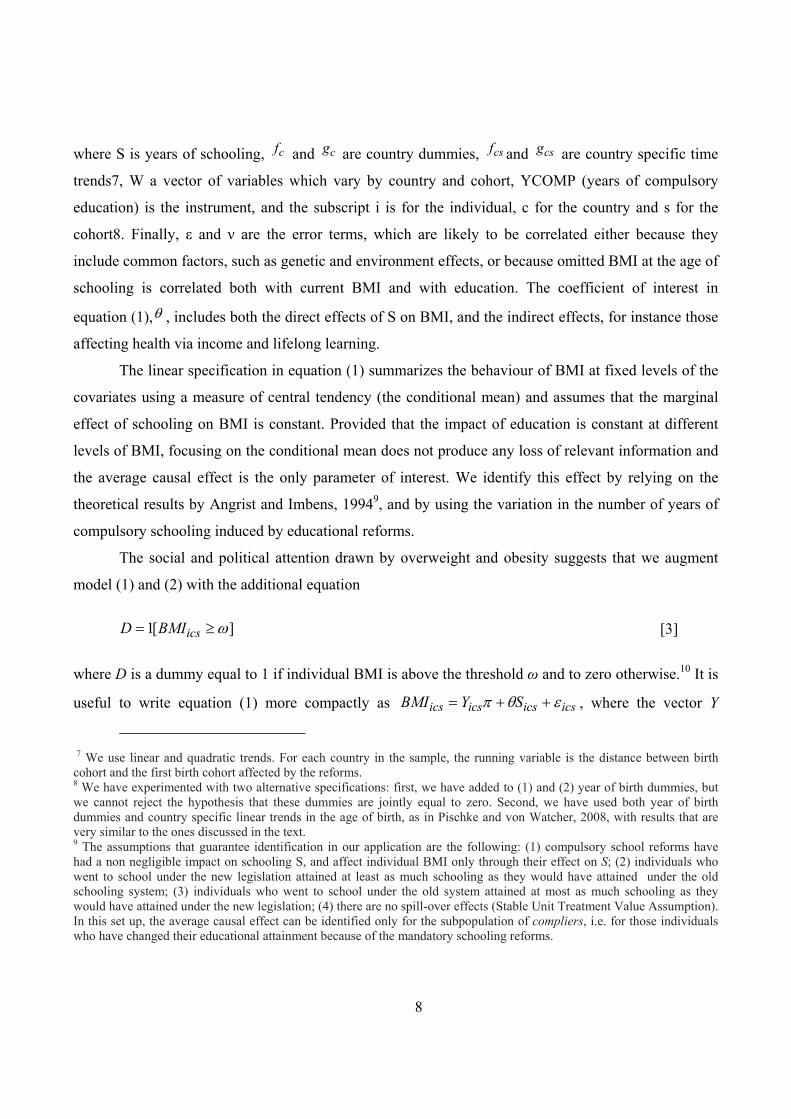
The linear specification in equation (1) summarizes the behaviour of BMI at fixed levels of the

covariates using a measure of central tendency (the conditional mean) and assumes that the marginal

effect of schooling on BMI is constant. Provided that the impact of education is constant at different

levels of BMI, focusing on the conditional mean does not produce any loss of relevant information and

the average causal effect is the only parameter of interest. We identify this effect by relying on the

theoretical results by Angrist and Imbens, 19949, and by using the variation in the number of years of

compulsory schooling induced by educational reforms.

The social and political attention drawn by overweight and obesity suggests that we augment

model (1) and (2) with the additional equation

][1 icsBMID [3]

where D is a dummy equal to 1 if individual BMI is above the threshold ω and to zero otherwise.10 It is

useful to write equation (1) more compactly as icsicsicsics SYBMI , where the vector Y

7 We use linear and quadratic trends. For each country in the sample, the running variable is the distance between birth cohort and the first birth cohort affected by the reforms. 8 We have experimented with two alternative specifications: first, we have added to (1) and (2) year of birth dummies, but we cannot reject the hypothesis that these dummies are jointly equal to zero. Second, we have used both year of birth dummies and country specific linear trends in the age of birth, as in Pischke and von Watcher, 2008, with results that are very similar to the ones discussed in the text. 9 The assumptions that guarantee identification in our application are the following: (1) compulsory school reforms have had a non negligible impact on schooling S, and affect individual BMI only through their effect on S; (2) individuals who went to school under the new legislation attained at least as much schooling as they would have attained under the old schooling system; (3) individuals who went to school under the old system attained at most as much schooling as they would have attained under the new legislation; (4) there are no spill-over effects (Stable Unit Treatment Value Assumption). In this set up, the average causal effect can be identified only for the subpopulation of compliers, i.e. for those individuals who have changed their educational attainment because of the mandatory schooling reforms.

9

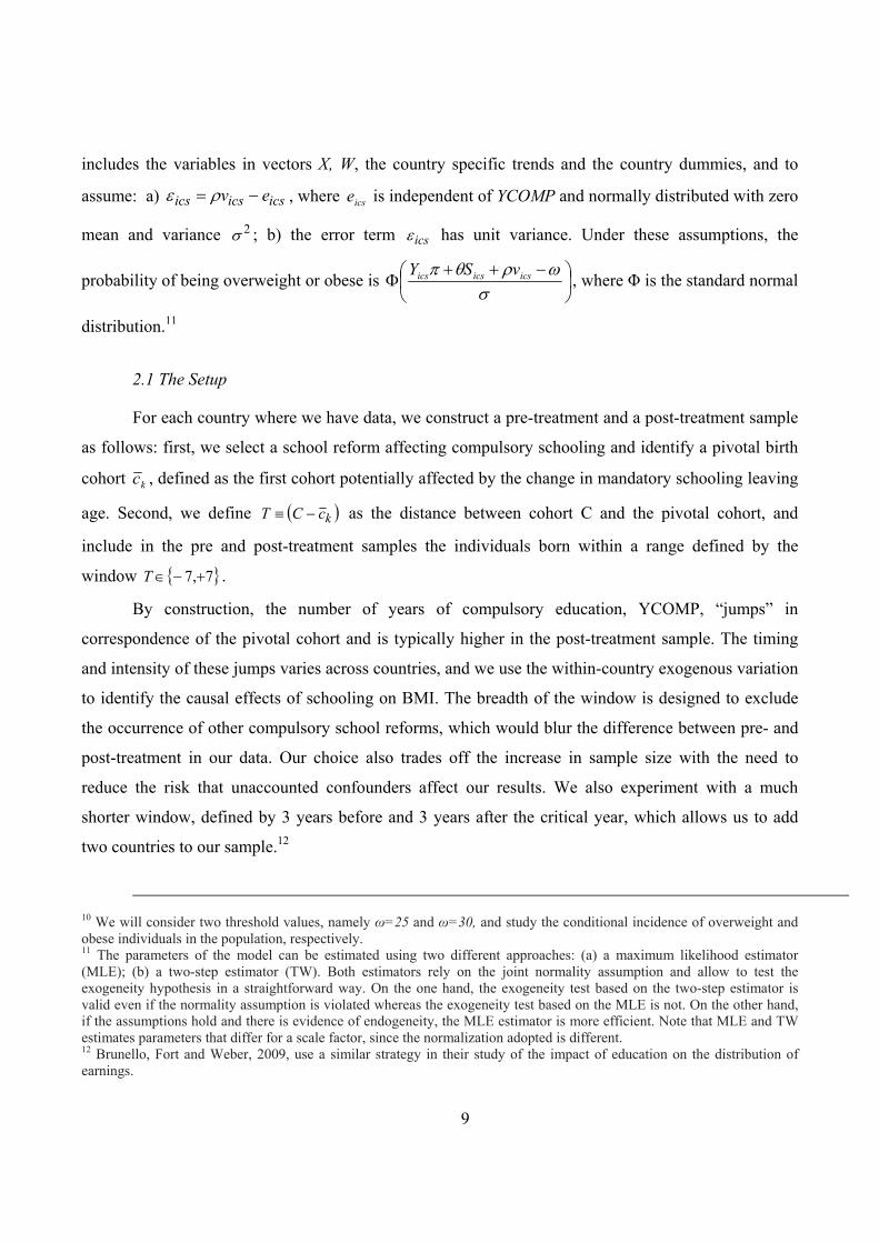
includes the variables in vectors X, W, the country specific trends and the country dummies, and to

assume: a) icsicsics ev , where icse is independent of YCOMP and normally distributed with zero

mean and variance 2 ; b) the error term ics has unit variance. Under these assumptions, the

probability of being overweight or obese is

icsicsics vSY, where Φ is the standard normal

distribution.11

2.1 The Setup

For each country where we have data, we construct a pre-treatment and a post-treatment sample

as follows: first, we select a school reform affecting compulsory schooling and identify a pivotal birth

cohort kc , defined as the first cohort potentially affected by the change in mandatory schooling leaving

age. Second, we define kcCT as the distance between cohort C and the pivotal cohort, and

include in the pre and post-treatment samples the individuals born within a range defined by the

window 7,7 T .

By construction, the number of years of compulsory education, YCOMP, “jumps” in

correspondence of the pivotal cohort and is typically higher in the post-treatment sample. The timing

and intensity of these jumps varies across countries, and we use the within-country exogenous variation

to identify the causal effects of schooling on BMI. The breadth of the window is designed to exclude

the occurrence of other compulsory school reforms, which would blur the difference between pre- and

post-treatment in our data. Our choice also trades off the increase in sample size with the need to

reduce the risk that unaccounted confounders affect our results. We also experiment with a much

shorter window, defined by 3 years before and 3 years after the critical year, which allows us to add

two countries to our sample.12

10 We will consider two threshold values, namely ω=25 and ω=30, and study the conditional incidence of overweight and obese individuals in the population, respectively. 11 The parameters of the model can be estimated using two different approaches: (a) a maximum likelihood estimator (MLE); (b) a two-step estimator (TW). Both estimators rely on the joint normality assumption and allow to test the exogeneity hypothesis in a straightforward way. On the one hand, the exogeneity test based on the two-step estimator is valid even if the normality assumption is violated whereas the exogeneity test based on the MLE is not. On the other hand, if the assumptions hold and there is evidence of endogeneity, the MLE estimator is more efficient. Note that MLE and TW estimates parameters that differ for a scale factor, since the normalization adopted is different. 12 Brunello, Fort and Weber, 2009, use a similar strategy in their study of the impact of education on the distribution of earnings.

10

Table 1 shows for each country in our sample the selected reform, the year of birth of the first

cohort potentially affected by the reform, the change in the minimum school leaving age and in the

years of compulsory education induced by the reform, the minimum expected school attainment,

expressed in terms of the ISCED classification, and the school entry age.13 The selected reforms

increased the minimum school leaving age by one year in Austria, Germany, Ireland, Britain and

Sweden; by two years in Denmark, France, Portugal and Spain; by three years in Finland, Greece, Italy

and by four years in Belgium. In some of these countries, namely Germany, Finland and Sweden, the

introduction of the reform varied by region. Since we do not have access to data at the municipality

level, for Finland and Sweden we define the year of the reform in each area as the year when the largest

share of municipalities in that area changed the schooling legislation. Notice that Northern and

Southern European countries are quite evenly distributed among early and late reforms.

3. The Data

We pool together data drawn from the 1998 wave of the European Community Household

Panel (ECHP), the second release of the first wave of the Survey on Household Health, Ageing and

Retirement in Europe (SHARE) for the year 2004, the 2002 wave of the German Socio Economic

Panel (SOEP), the 2003 wave of the British Household Panel Survey and the 2003 wave of the French

Enquete sur la Sante.14 The countries included in this dataset are: Austria, Belgium, Denmark, Finland,

France, Germany, Greece, Ireland, Italy, Portugal, Spain, Sweden and the United Kingdom. In the case

of a few countries, we use data from two different surveys.

Since Portugal experienced a second school reform in 1968, four years after the 1964 reform,

the window of observation for this country is only the shortest one (three years before and after the

critical cohort). Swedish data are from SHARE, and have a small number of observations at the upper

tail of the longer window. Because of this, we include this country only in the shortest window.

Finally, we exclude from the sample individuals younger than 25, who are likely to be still in

education, and those older than 65. This implies that Belgium, where the compulsory school reform

took place in the early 1980s, is included only with the shortest window.

13 See Brunello, Fort and Weber, 2009, for details on the sources of these data. 14 The ECHP is a panel of European households. We choose the 1998 wave so as to maximize the number of observations in the sample. These data do not contain information on BMI for key countries such as France, Germany and the UK. For these countries we select national surveys, using waves that include information on BMI.

11

Our dependent variable is the body-mass index (BMI), defined as weight in kilograms divided

by the square of height in meters (kg/m2). The BMI, albeit somewhat crude, has been found to be

highly correlated with more precise (and more costly to collect) measures of adiposity.15 In all our data

sources individual height and weight are self-reported. As such our measure of BMI may be affected by

measurement error, with heavier persons more likely to underreport their weight (see Burkhauser and

Cawley, 2008). Notice however that Sanz-de-Galdeano, 2007, finds that the rank correlation between

country level self-reported and objective measures of weight is very high. Following Hamermesh,

2009, we only consider females with BMI in the range 15 to 55.

In Sections 4 and 6, we measure educational attainment with the number of years of schooling.

For all countries in the sample except France, this number is based on responses to questions asking the

age when full time education was stopped and the highest level of education was attained. In the case

of France, we attributed to each individual in our sample the average years of education spent by her

cohort to complete the attained degree, as measured in the Enquete sur l'Emploi. Table 2 reports

average BMI, years of schooling, years of compulsory education, age and the number of observations

in the sample by country. Average BMI is equal to 24.67, close to the 60th percentile. Since median

BMI is 23.87, the unconditional distribution is not symmetric. Average age is highest in Austria,

Germany, Italy and France, because the relevant reforms occurred in the 1950s and 1960s. Years of

schooling depends on birth cohort and is highest in the UK and Belgium and lowest in Italy and

Portugal.

To identify the causal relationship between education and BMI we need to control as accurately

as possible for additional factors affecting the dependent variable. We include in the empirical

specification both country and survey dummies. Furthermore, trend-like changes in both education and

BMI relative to the time of the school reform are controlled with a second order polynomial in K=T+7

– where T is the distance between each cohort and the first cohort potentially affected by the reform -

and its interactions with country dummies16.

15 Other anthropometric methods for measuring individuals body fat include the waist-hip ratio, sagittal abdominal diameter, skin folds thickness. More accurate measures are based on bioelectrical impedance analysis, infrared interactance, dual energy X-ray absorptiometry. All these methods imply some instrumental measurement that is usually far from being viable in social surveys. 16The relatively low order of the polynomial follows the suggestions by Lee and Card, 2008. Compared to higher order polynomials, the second order specification is the most parsimonious and provides adequate fit of the data. The country specific trends may help capture the effects of unmeasured school quality on BMI. Following Lee and Barro, 1997, one way to improve our ability to control for school quality is to compute measures of the pupil – teacher ratio in secondary schools

12

Recent empirical research has documented that adult BMI is correlated to weight at birth, and

that the latter is correlated to the season of birth and the climatic conditions prevailing at the time of

birth (see for instance Phillips and Young, 2000; Murray et al, 2000; van Hamswijck et al, 2002). We

use individual information on the month and year of birth to construct two variables: 1) a dummy equal

to 1 if the individual is born in autumn or winter, and 0 otherwise; 2) the average temperature

registered in the country during a window spanning three months before and after birth. Data on

historical temperature for each country come from the Global Historical Climatology Network monthly

data base, made available by the National Climatic Data Center at the US Department of Commerce.

Changes in educational attainment after a compulsory school reform could be due to the reform

itself or to confounding factors, which may alter the incentives to invest in education at the time of the

reform but independently of it. To illustrate, take a reform that increases the minimum school leaving

age from a to a+1 in a certain year. If individuals at age a - or their parents - find it more attractive to

invest in education because of a reduction in the opportunity costs generated by a contemporaneous

increase in the unemployment rate, they might invest more independently of the reform. To control for

this, we include in the vector W of equation [1] the female unemployment rate (by country) and the

country specific real GDP per head at time b+a, where b is year at birth. Both GDP per capita and the

unemployment rate near school reforms are likely to affect BMI also because they influence health

conditions and school quality at the time when critical schooling decisions are taken.

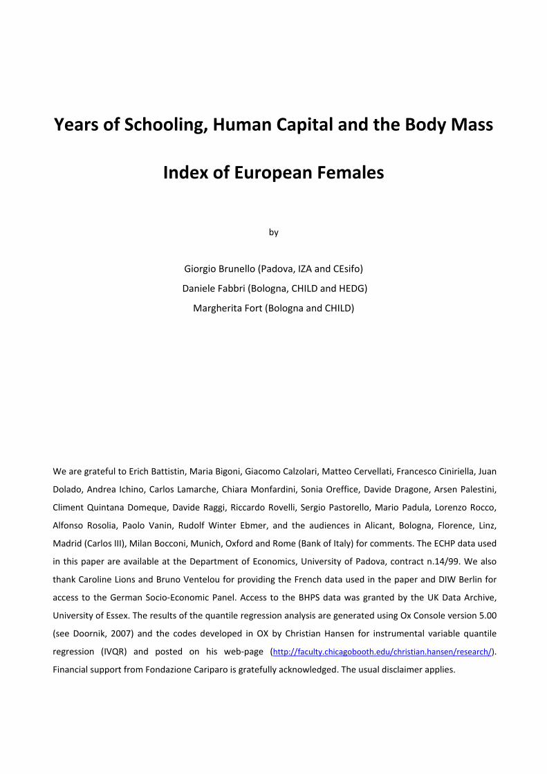
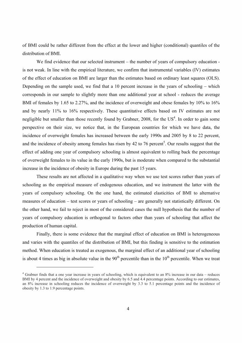
Figure 1 presents the cumulative distribution function of years of education both for the cohorts

affected (broken line) and for the cohorts not affected by the reforms (continuous line). It is clear that

the empirical distribution shifts to the right after the reforms, suggesting that the proportion of

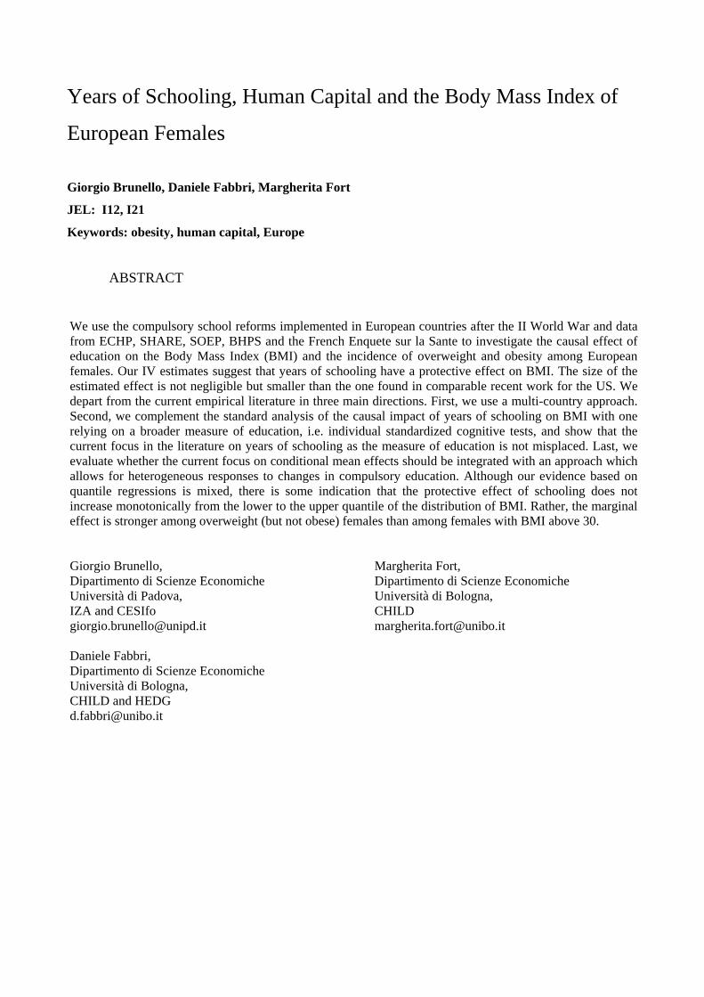
individuals attaining relatively low education declines among the younger cohorts. To check whether

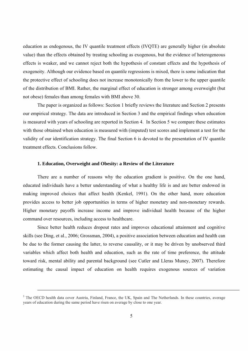
this shift is partially induced by compulsory school reforms, we purge years of schooling from the

influence of exogenous controls and cohort effects and plot the residuals in Figure 2 for the cohorts

born before and after the first cohort potentially affected by the reforms. The upward jump at the time

of the reforms is clearly visible and corresponds to about 0.4 years for each additional year of

mandatory schooling prescribed by law.17

in the neighbourhood of the time when school reforms took place. Unfortunately, the available data do not cover in a satisfactory way the full set of countries available in our dataset. 17 Figure 1 is based on the sample of individuals born 7 years before and 7 years after the critical cohort and excludes data from Belgium, Sweden and Portugal. This jump is slightly larger than the one found by Brunello, Fort and Weber, 2009,

13

4. The Effects of Schooling on BMI

Table 3 reports the first stage estimates of years of schooling on the vector of exogenous

variables plus the instrument YCOMP for two time windows, our baseline window [+7,-7] (column 1 in

the table) and the shorter window [+3,-3] (column 2). We find that our instrument is significantly

correlated with the endogenous variable. As anticipated by Figure 2, one additional year of compulsory

education increases the years of schooling attained in our sample by close to 0.4 years. We test for the

presence of weak instruments by comparing the F-statistic for the exclusion of YCOMP from the first

stage regressions with the rule of thumb indicated by Staiger and Stock, 1997, which suggests that the

F-test should be at least 10 for weak identification not to be considered a problem. In all specifications,

we can reject the hypothesis that our instrument is weak, albeit only marginally in the shorter

window18.

Table 4 presents the ordinary least squares (OLS) and instrumental variables (IV) estimates in

the two selected windows. The estimated association between BMI and years of schooling is negative.

With OLS, the size of the effect is similar to that estimated by Cutler and Lleras-Muney, 2007, for US

whites aged over 25 (-0.190) but smaller than the estimate for US females (-0.302) reported by

Grabner, 2008. The IV estimates of the impact of years of schooling on BMI are always larger in size

than the OLS estimate – a standard result in this literature19, see Grabner, 2008, for a discussion - and

statistically significant at the 5 percent level of confidence. Our results imply that a 10 percent increase

in years of schooling reduces the BMI of females by 1.65 in the broader window and by 2.27 percent in

the narrower window, a moderate effect when compared to the 4 percent decline estimated by Grabner

for the US, using compulsory school reforms to instrument years of schooling, as we do20.

Turning to the other regressors in Table 4, we find no evidence that the average temperature at

birth influences individual BMI after controlling for the semester of birth. There is instead weak

evidence that individual BMI is lower among individuals born in autumn and winter, and that a higher

GDP per capita at the age first affected by the reforms reduces individual BMI. Our interpretation of

who consider however only employed individuals. Here we include in our sample all females independently of their labour market status. 18 Even though just – identified 2SLS estimates are approximately unbiased, a weak instrument may lead to imprecise estimates in the second stage (Angrist and Pischke, 2009). 19 This could be due to a common unobserved factor inducing a positive correlation between education and BMI. A possible interpretation of our result is that better educated individuals report weight more correctly. 20 When interpreting the IV estimates in Table 4, it is important to notice that the Hausman test never rejects the null of exogeneity of years of schooling.

14

these findings builds on two observations. First, our dependent variable is adult BMI – measured as the

ratio between weight and height squared. Second, evidence in the literature suggests that when the

economy strengthens there is a transient increase in BMI (see Ruhm, 2000 and 2003) but a permanent

increase in height (see Van den Berg, et al. 2009). Therefore, ceteris paribus, individuals exposed to

early good economic environments tend to be taller but not necessarily heavier when adult. The

estimates reported in Table 4 also suggest that, other things being equal, the higher the female

unemployment rate at the age the individual was first affected by the reforms the lower her BMI when

adult. In other words, cohorts of women whose mothers were more probably not working at the time of

the reform tend to be leaner at adult age.

4.1 The Effects of Schooling on the Probability of Being Overweight and Obese

We estimate probit models by treating schooling either as exogenous (columns 1 and 3 of Table

5) or as endogenous (columns 2 and 4 of Table 5)21. In the latter case, we use years of compulsory

schooling as instrument. In the case of overweight, and depending on the selected window, the

evidence suggests that a 10 percent increase in years of schooling (slightly more than 1 year from the

sample mean) reduces the probability of being overweight by 6.71 to 6.82 percent when schooling is

treated as exogenous and by 10.87 to 16.60 percent when it is treated as endogenous. Concerning

obesity, IV estimates are imprecise and close to standard probit estimates. In this case, a 10 percent

increase in years of schooling reduces obesity by 11.57 to 16.70 percent when years of schooling are

treated as endogenous, depending on the window. The Wald test on the exogeneity of schooling never

rejects the null.

The comparison of the conditional mean effects in Table 4 with the estimates in Table 5 is

informative of the presence of heterogeneous effects of schooling on BMI at different points of the

distribution. To illustrate why, consider the overweight and the broader window of observation. If the

effects of one additional year of schooling were the same across the distribution of BMI (i.e. -0.35),

only the individuals who had before the increase a BMI between 25 and 25.35 would cease to be

overweight because of the policy. Since this group is 2.43 percent of the relevant population, the

percentage of overweight individuals would decline by the same amount, but below the estimated

decline (-4.41 percentage points, the marginal effect reported in column 2, Table 5 panel a). It follows

15

that the findings in Tables 4 and 5 (for the overweight) are consistent only if the marginal effect of

higher schooling on BMI is larger among those currently overweight.

We can apply a similar argument to the obese and the sample with the broader window. In the

case of a homogeneous effect of one additional year of schooling, only those with BMI between 30 and

30.35 would cease to be obese after the policy, which corresponds to 1.04 percentage points. This

percentage is very close to the one we estimate (-1.2 percentage points, see column 2, Table 5 panel b),

which suggests that the effect (in absolute value) of additional schooling on BMI is quantitatively

lower for the obese than for the overweight. These considerations suggest that the extent of the

marginal response of BMI to schooling does not increase monotonically as we move from the mean to

the upper quantiles of the distribution of BMI: presumably, the response is larger in absolute value for

the individuals located in the 70th and 80th percentiles, and smaller for those in the 90th percentile –

where most of the obese are located.

5. Checking the Validity of the Exclusion Restriction: the Effects of a Broader Measure of

Education on BMI

In the empirical literature on the causal effects of education on health, it is customary to

measure the former with years of schooling, thereby ignoring important dimensions of education, such

as school quality and learning from labour market experience, which includes training. In this section,

we take a broader view of education by considering the effects on BMI of cognitive skills, as proxied

by cognitive test scores (TS). As argued by Hanushek and Wossmann, 2009, in their empirical study of

growth, one of the advantages of using cognitive skills as a measure of human capital is that it allows

for “…differences in performance among students with differing quality of schooling (but possibly the

same quantity of schooling)….[and opens]…the investigation of the importance of different policies

designed to affect the quality aspect of schools.” (Hanushek and Wossmann, 2009, p. 6).

There is another important reason why we consider cognitive skills in this paper: in our set up

the (internal) validity of the identification strategy requires that the instrument YCOMP does not affect

BMI directly but only through education (exclusion restriction). This requirement is more likely to be

met when we use a broader measure of education than simply years of schooling. We show that, under

21 Since the two-step estimates obtained with the standard control variate approach (Wooldridge, 2002) give results similar to the maximum likelihood estimates (obtained with the STATA code IVPROBIT), we do not report them here.

16

some mild additional assumptions, the availability of such measure – test scores - provides a way of

testing the validity of the exclusion restriction when education is measured with years of schooling, as

usually done in the empirical literature.

5.1 The Test

To illustrate the implications of using test scores rather than years of schooling as a measure of

education, assume that TS is generated by equation [4], where Q is a “catch all” variable which is

orthogonal to S and includes the effect of factors other than S on TS (school quality, parental

background and learning from experience)22

),( SQFTS [4]

Let the "true" relationship between BMI and education be given by

vTSBMI [5]

where the effects of the variables in vector Y have been partialled out, and let IV be the IV estimate

when compulsory school reforms are used as instruments for test scores. This estimate is consistent if

0),( vYCOMPCov , which we treat as our maintained hypothesis. Assuming that equation [4] is linear

in S and Q

QSTS 210 [6]

we can use [6] into [5] and obtain the relationship estimated in the empirical literature

SBMI [7]

where 1 and vQ 20 .

Under the maintained hypothesis, IV is consistent but the IV estimate of α, IV , fails to be

consistent if the selected instrument is correlated with omitted Q. When this is the case, it is

inappropriate to estimate the relationship between education and BMI using years of schooling as

22 Since school quality and lifelong learning may be correlated with years of schooling, it is useful to think of Q as a residual “catch all” variable after S has been partialled out.

17

measure of education – as in [7] – and a broader measure – such as test scores – should be adopted, as

in equation [5]. In order to test whether restricting education to years of schooling – as done in the

empirical literature so far – can deliver consistent IV estimates of the causal effect of education on

BMI, consider the null hypothesis: a) the instrument YCOMP does not affect Q;

b))(

),(

)(

),(2 TSV

vTSCov

QV

vQCov . Under this (joint) hypothesis, we show in the Appendix that:

1

][

][][

][

IV

IV

OLS

OLS

E

EE

E

[8]

This result holds because: (a) under the null hypothesis the OLS estimators in the two models

have the same bias, and both the IV estimators are asymptotically unbiased; (b) the rescaling factor 1

is the same when we contrast OLS or IV estimates. Importantly, condition [8] is sufficient but not

necessary. Hence, we may reject it even if the orthogonality condition ),( YCOMPQCov does not fail,

but the auxiliary assumption that the ratio of the covariances of Q and TS with the error term v be

proportional to the ratio of the variances, with factor of proportionality equal to 2 , fails to hold.

Therefore, the test is conservative23.

It follows that, when there are two measures of human capital (TS and S) and one instrumental

variable that can be used in turn for either endogenous variable, we can test the hypothesis that the

identification strategy is valid in both cases by comparing the ratio of the OLS and the ratio of the IV

estimates in the two specifications. If the null hypothesis [8] is not rejected, we interpret this as

evidence that the exclusion restriction is met. In this case, using years of schooling as the measure of

education and years of compulsory schooling as the instrument for endogenous education produces

consistent IV estimates of the causal relationship between education and BMI.

5.2 The Data on Test Scores

Our measure of cognitive skills is drawn from the International Adult Literacy Survey (IALS),

which tests individual cognitive skills in the population aged 15 to 65 and in different countries

23 In the Appendix we use simulations to show that the proposed test has enough power to reject the null hypothesis.

18

according to a common, standardized format24. The approach followed by IALS is to measure cognitive

skills in three domains – quantitative literacy, prose literacy, and document literacy. The former is

defined as the ability to apply “arithmetic operations, either alone or sequentially, to numbers

embedded in printed materials”. Prose literacy is defined as the ability to understand and to use

“information in texts”. Document literacy is defined as the ability to “locate and use information in

various formats” (see Cascio, Clark and Gordon, 2008). Cognitive skills as measured by IALS test

scores reflect both the formal education process – its quantity and quality - and the learning activities

taking place after education is completed. Therefore, they are a good proxy of the stock of cognitive

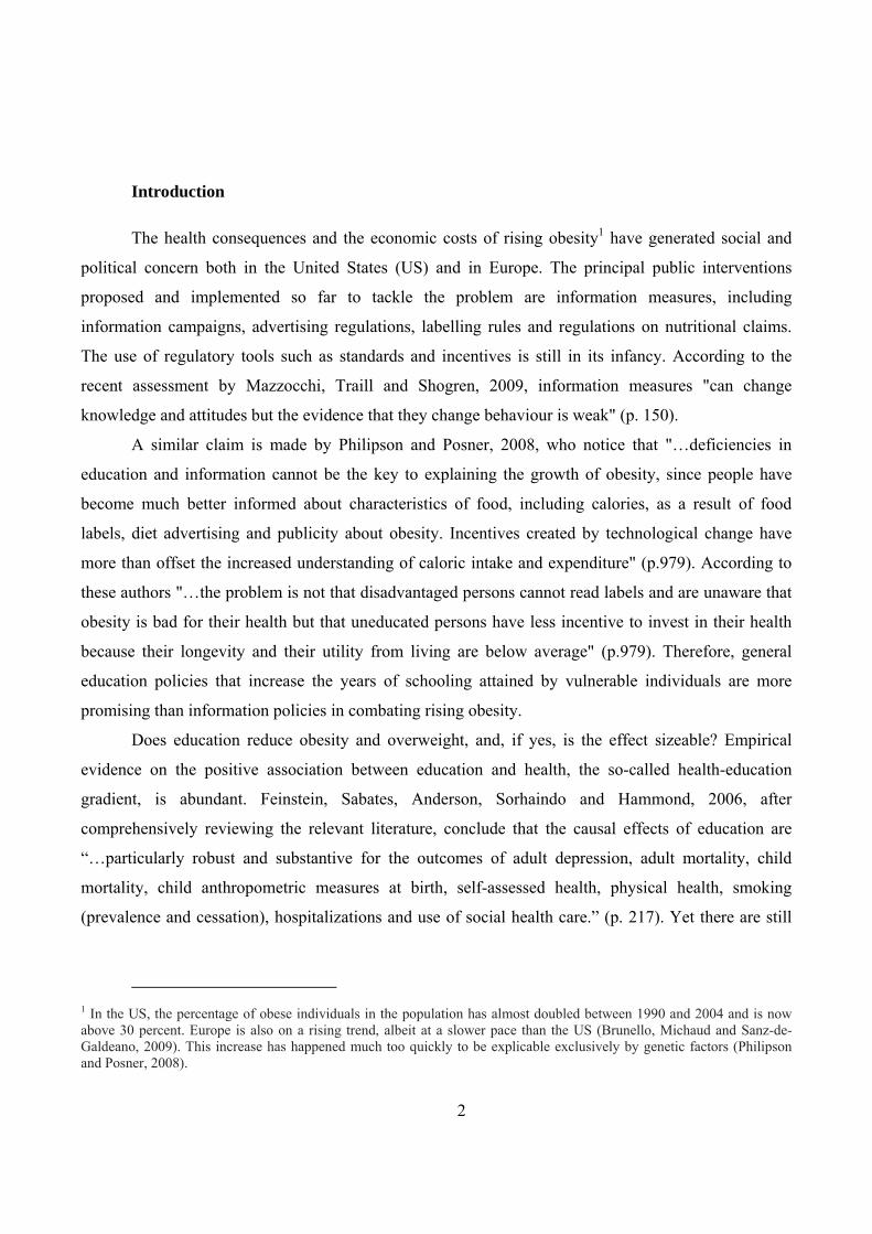
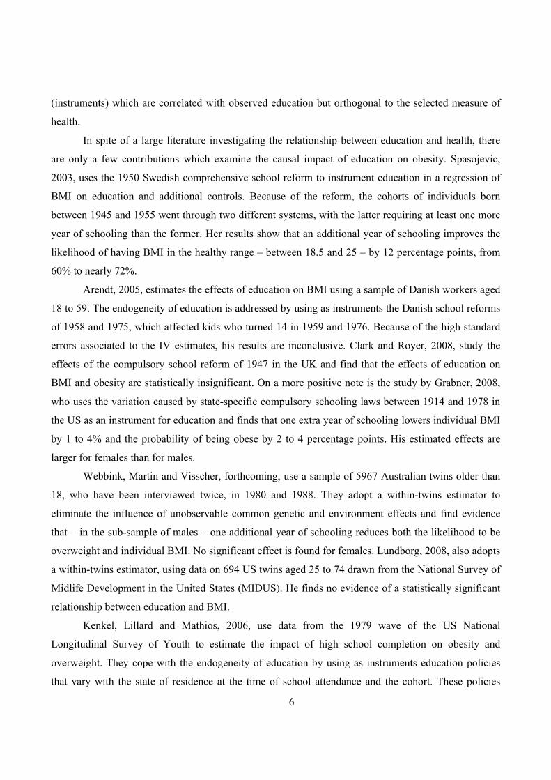
human capital accumulated by each individual until the time of the interview. The data document both

the positive association between education and test scores and the substantial variation in test scores for

a given number of years of schooling (see Figure 3), which can be driven by differences in parental

background, school quality and learning from labour market experience.

5.3 The Imputation Procedure

The implementation of the test requires information on the following variables: individual BMI,

education - both quantity and quality - country and year of birth.25 Our main dataset (the “FULL

sample” hereafter) has all the required information, with the exception of test scores. On the other

hand, the IALS dataset includes all relevant variables but BMI. Since IALS and the FULL dataset are

drawn from different samples, we develop an imputation procedure which allows us to augment our

original dataset with information on test scores, limitedly to the countries that are included in both

samples.

Within each country and in both datasets, the available data are a representative random sample

of the same population. Starting from this observation, we combine information from both sources and

construct a new sample which includes two distinct measures of the quantity of education, the one

24 This is the source of international test scores best suited to our purposes, both because it covers the adult population and because it was carried out in the second part of the 1990s, when most of our data on BMI are collected. Other international surveys of cognitive skills typically focus on the population at schooling age. For instance, the Trends in International Mathematics and Science Study (TIMSS) covers mainly 13 year old students, and the OECD Programme for International Student Assessment (PISA) focuses on 15 year old pupils. An alternative option would have been to use the test scores included in the SHARE dataset. However this option is not viable in the current setup because of the limited number of observations available for each relevant cohort and country. 25 The last two variables are crucial for the definition of our instrumental variable.

19

recorded in IALS (we call it IALSS ) and the one recorded in the FULL dataset (call it FULLS ), the test

score and the BMI. This is done in three steps.

First, we restrict the FULL sample to the sub-sample of countries also surveyed by IALS. This

sub-sample includes Denmark, Ireland, Italy and United Kingdom when we consider individuals born

within the range of 7 years before and after the pivot cohort in each country. Second, we define strata

in the FULL sample as consisting of individuals from the same country, born in the same year and with

identical levels of education (as measured by FULLS ). Finally, we attach to each individual in the FULL

sample the information on the education profile (quantity of education IALSS and test score) of a

randomly chosen individual from the IALS sample who is born in the same year, the same country and

reports roughly the same level of education, as recorded by FULLS .26 In other words, for any given

stratum in FULL the corresponding set of "donors" (observations used to donate a missing variable) in

IALS is made of individuals of exactly the same age and country and with years of education that fall

within a given tolerance interval around FULLS .

We consider three different tolerance levels as constant percentage variations around a given

value of FULLS : high (30%), medium (25%) and low (20%) tolerance. To illustrate, consider Italian

females in the FULL sample who have 8 years of schooling and are born in 1955. The relevant sample

of IALS donors in this case is made of Italian females born in the same year and with IALSS between

5.6 and 10.4 years (high tolerance), 6 and 10 years (medium tolerance), and 6.4 to 9.6 years (low

tolerance). In the definition of tolerance levels, we face the following trade-off: on the one hand, the

lower is the tolerance level, the higher is the correlation between years of schooling in different

samples. On the other hand, the lower is the tolerance level, the smaller is the number of observations

in each stratum and the larger is the number of empty strata.27

Table A1 reports the pair-wise correlation coefficients between IALSS , FULLS and test scores in

the generated sample for the three levels of tolerance. As expected, the lower is the tolerance level, the

higher is the observed correlation between different measures of schooling. Table A2 reports sample

sizes by country and survey: the ratio of individuals in IALS with respect to FULL is 94/100 in the UK,

63-66/100 for Denmark and Ireland and 20/100 for Italy. Figure A1 includes the scatter plots of actual

26 By so doing we attach the joint distribution of IALSS and the test score.

20

and imputed years of schooling for the three different levels of tolerance. As documented in Figure 3,

our imputation method is able to reproduce rather well in the FULL sample the variation in test scores

for each year of schooling that is observed in the IALS sample.

5.4 The Estimates

Table 6 shows for alternative tolerance levels the OLS and IV estimates when the explanatory

variable is either years of schooling or test scores, and the sample consists of four countries (Denmark,

Ireland, Italy and the UK) in the broader window [+7,-7]. It turns out that the IV point estimates of the

effects of years of schooling on BMI are rather close to the estimates in the main sample (see Table 4),

within the range [-0.446, -0.421] using FULLS and within the range [-0.544,-0.526] using IALSS . On the

other hand, the estimated marginal effect of test scores is in the range [-0.030, -0.027].

When we compare estimated elasticities rather than marginal effects, we find that the elasticities

of BMI to years of education and test scores are rather similar, and range between -28% and -19% in

the former case and between -27% and -31% in the latter case. We use the estimates in Table 6 to

compute the two statistics )(

)(/

)(

)(1

IV

IV

OLS

OLS

E

E

E

Et

and S

BMI

TS

BMIt

ln

ln

ln

ln2

and to test whether these

statistics are different from one and zero respectively. In this exercise, we consider the OLS and IV

estimates of when years of schooling are equal to either IALSS or FULLS .28 The results are reported

in Table 7 ( IALSS ) and Table 8 ( FULLS ). In the former case, the hypotheses 11 t and 02 t are never

rejected at the 5% or 10% level of confidence. In the latter case, we reject 11 t only when we use data

with relatively high tolerance (30%) and we reject 02 t at 5% for medium and high level of tolerance.

Overall, these results suggest that using years of schooling as the measure of education when

investigating the relationship between education and BMI does not produce inconsistent IV estimates.

This is particularly important in the light of the fact that datasets which include both measures of health

lifestyles such as BMI and alternative measures of education – such as years of schooling and test

scores – are rather uncommon. Our findings also point out that, once we have controlled for the direct

and indirect effects of years of schooling and we have instrumented years of schooling using the years

27 We have considered tolerance levels, spaced 0.05, in the interval [0.05,0.30]. The fraction of matched records corresponding to each tolerance level is 89%, 93%, 97%, 98%, 99% and 99% respectively. We restrict our attention to the three cases where the fraction of matched records is above or equal to 98%. 28 The standard errors and confidence intervals for 1t and 2t are obtained by bootstrapping (500 replications).

21

of compulsory schooling, the contribution of the residual “catch all” variable Q to individual test scores

TS and BMI is negligible and not significantly different from zero29.

6. Quantile Treatment Effects

In this final section, we investigate the effects of education on the shape of the conditional

distribution by modelling each conditional quantile ),|(,| SYQ SYBMI as:

icsicsSYBMI SYSYQ )()(),|(,| [9]

where is the th -quantile, )( is the parameter of interest and years of schooling S are treated as

endogenous. An appealing feature of equation [8] is that it nests the location shift model of equation [1]

(see Koenker, 2005), and allows at the same time to study how education affects the different quantiles

of the distribution of BMI, including those where overweight and obese individuals are concentrated.

We estimate IVQTE (instrumental variable quantile treatment effects) by adopting the approach

proposed by Chernozhukov and Hansen, 2005,30 which applies to the whole (treated) population, and is

based on imposing some structure to the evolution of ranks across treatment states. Their approach is

applicable when the outcome variable is continuous, while both the endogenous variable and the

instrumental variable can be either continuous or discrete. Let )1,0(UU be the latent factor (or rank

variable) responsible for the heterogeneity of outcomes for individuals with the same Y and S. It is

convenient to call this factor “nature and nurture”. The critical assumption in this approach is that,

conditional on the instrument Z, the distribution of the rank variable does not vary with the treatment S

29Notice that in our setting the statistic t2 has the following expression:

QBMI

STSBMIBMI

S

BMI

TSt

IVIVIVIV

2012

ˆˆˆˆ . Provided that cognitive abilities, as proxied by TS,

are "produced" according to equation [6], our estimates suggest that the contribution of 0 + Q2 is negligible. 30 Abadie, Angrist and Imbens et al, 2002, generalize the approach by Angrist, Imbens, 1994, to the estimation of the effect of a binary (potentially endogenous) treatment on the quantiles of the distribution of a scalar continuously distributed outcome. Since this approach has not yet been extended to the case where the endogenous variable is either discrete or continuously distributed, it is not well-suited to the application at hand, where education is measured in years of schooling, a discrete variable. Chesher, 2003, uses a recursive model with a triangular structure both in the observable and in the latent variables. The latter assumption is problematic in our context, because the error terms in equations [1] and [2] are likely to contain common factors, such as genetic and non-genetic environment effects.

22

(rank similarity). In our setup, this is equivalent to saying that the treatment does not alter the ordering

induced by genetics and early life conditions ("nature and nurture")31.

In practice, the estimation requires two steps (see Chernozukhov and Hansen, 2006): first, we

use tentative estimates of ),|(,| SYQ SYBMI to estimate quantile regressions of ),|(,| SYQBMI SYBMI

on Y and the instrument YCOMP; second, we choose as the estimate of the coefficient )( the one

which minimizes the absolute value of the coefficient of YCOMP in the first step. This procedure

requires an initial estimate of ),|(,| SYQ SYBMI in the first step. Chernozhukov and Hansen consider

linear quantile regression models and suggest to use a grid search for )( , centered around the two

stage quantile regression estimates – i.e. quantile regressions of BMI on S* and Y, where S* is the

expectation of S conditional on Y and the instrument YCOMP 32.

In this empirical implementation, we consider only the FULL sample with the broader window

(-7,+7), and a range of equally spaced quantiles over the interval [0.1, 0.9]. We report the estimates for

nine deciles only for brevity: while Table 9 shows the results under the null of exogenous education,

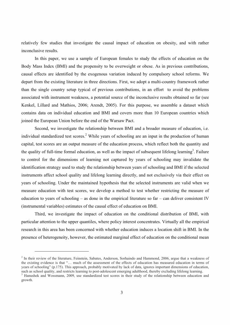
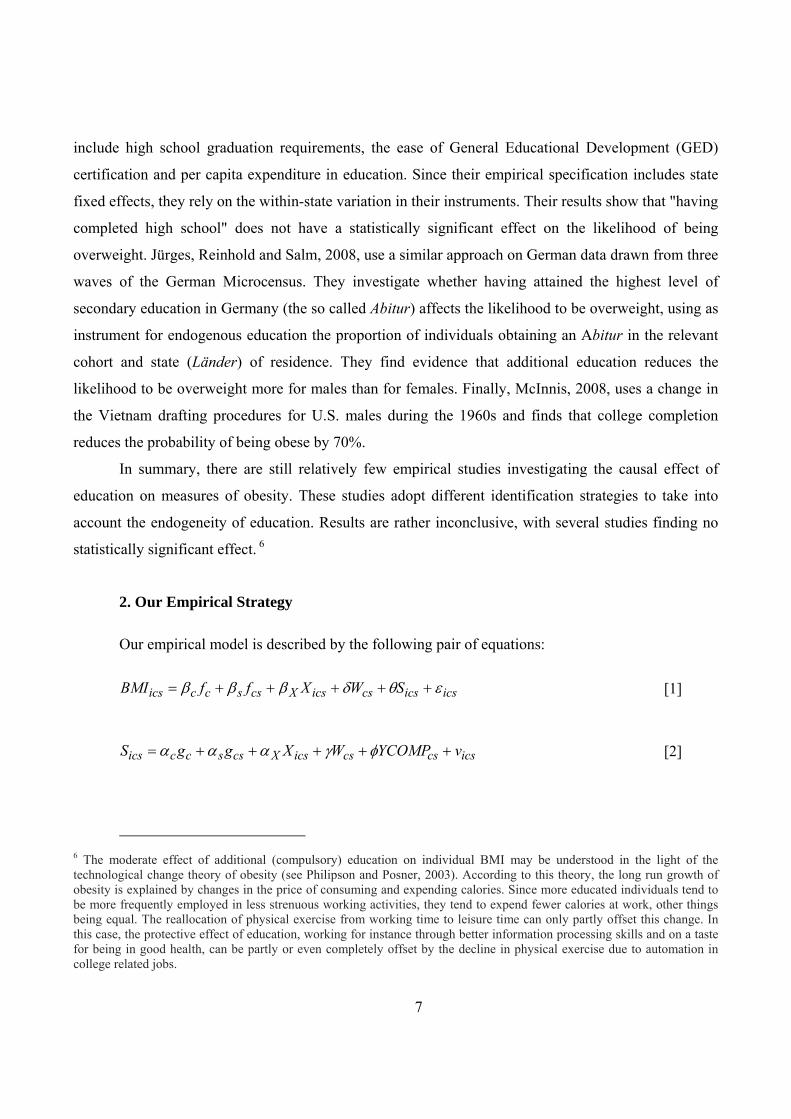
Table 10 presents the findings when we use the Chernozhukov and Hansen IVQTE model. Figure 4

shows how the estimated coefficients of years of education (top panel) and the intercept (bottom panel)

vary as we move from the lowest to the highest quantiles on the conditional distribution of female BMI.

Each dot in the graphs represents an estimated coefficient and the shaded area shows the 95%

confidence interval around the estimate. In the estimates reported in this figure, education is treated as

exogenous. The intercept measures the conditional quantiles of BMI for the baseline country, the

United Kingdom, when all the continuous regressors are set at their sample mean and years of

education are set to zero. The estimated level of BMI is around 20 at the bottom (0.10) quantile, raises

to 25 at the third decile, is around 28 at the median and reaches 37 at the highest quantile (0.90). We

contrast these estimates with those obtained when treating education as endogenous – see Figure 5. In

the upper part of the figure, we show the IV estimates only for nine deciles; in the bottom part, we

present instead the estimates when all the quantiles are used.

31 The rank similarity assumption is the (un-testable) identifying assumption in the model proposed by Chernozhukov and Hansen, 2005. This assumption is not required under the approach proposed by Abadie, Angrist and Imbens, 2002. 32 We implement the method proposed by Chernozhukov and Hansen and estimate quantile treatment effects when education is treated as endogenous by adapting to our application the OX algorithm provided by Hansen in his web-page. The algorithm uses a fixed search grid. The results are equivalent to those obtained using a search grid centered around the two stage quantile regression estimates provided the grid step is sufficiently narrow.

23

When schooling is treated as exogenous (Table 9), there is evidence that its negative correlation

with BMI increases in absolute value as we move from the bottom to the top quantiles: the marginal

effect of an additional year of formal education is around -0.08 at the first decile, -0.18 at the median

and -0.26 at the eight decile (the corresponding effect at the conditional mean is –0.20, see column 1 in

Table 4). A test of the hypothesis that the estimated correlations are not statistically different across the

nine selected quantiles of BMI clearly rejects it at the 1% level of significance.33 The observed pattern

supports the view that raising education could be particularly beneficial to overweight and obese

individuals.

When education is treated as endogenous (Table 10) and we use IVQTE with years of

compulsory education YCOMP as the instrument, we find that the causal effects of schooling on BMI

are larger in absolute value than the associations shown in Table 9, but often imprecisely estimated.

Moreover, there is no clear monotonic pattern in the estimated marginal effects, which are larger for the

quantiles in the range 0.5-0.8 and lower elsewhere, including at the 9th quantile. These results are in

line with those discussed at the end of sub-section 4.1, which are based on the estimates of the

probability of being overweight and obese34: there are signs that the effects of schooling are

heterogeneous along the distribution of BMI, but their absolute value does not increase monotonically

as we move from the bottom to the top quantiles. Rather, the marginal effect of additional (compulsory)

education on BMI is larger for overweight than for obese females, who are arguably the primary target

of public intervention.

Conclusions

In this paper, we have departed from the empirical literature which investigates the effects of

education on the body mass index in three main directions. First, we have adopted a multi-country

33 The Wald test statistic is equal to 22.53, with a p-value of 0.000. We tested the hypothesis that education affects only the location of the conditional distribution of BMI, i.e. that the effect is homogeneous, by considering also a variant of the Kolmogorov-Smirnov test based on the quantile regression process (see Koenker, 2005 for details). We run the test using a routine available in the software R. The observed test value is 2.102. We contrast this with the asymptotic critical values provided by Koenker, 2005 (Table B.1 p.318), i.e. 2.640 (1%) 2.102 (5%) 1.833 (10%). Since the test rejects for values higher than the critical value, we do not reject the null at 1% , the test is inconclusive at 5% and rejects at 10%. 34 By relying on estimates of the quantile regression process at equally spaced quantiles, we test formally the following hypotheses: (1) the effect of education is not statistically different from zero at all conditional quantiles; (2) the effect of education on BMI has the same negative sign over the whole distribution (education is protective); (3) the exogeneity of years of schooling. While we reject at the 5% level of confidence the hypothesis that the effect of education on the

24

framework rather than the single country setup typical of previous contributions, in an effort to avoid

the problems associated with instrument weakness. Second, we have investigated the relationship

between BMI and a broader measure of education, i.e. individual standardized test scores, which

capture the output of the production of individual human capital rather than a single input. Third, we

have studied the impact of education on the conditional distribution of BMI, with particular attention to

the upper quantiles, where policy interest concentrates.

Our empirical findings point to three main conclusions: first, education has a protective effect

on BMI and the probability of being obese or overweight. The size of the estimated effect is not

negligible but smaller than the one found in recent comparable estimates for the US. Second, and

reassuringly, we cannot reject the hypothesis that the standard usage of years of schooling as the

measure of endogenous education –instrumented with compulsory years of schooling - produces

consistent estimates. There is also evidence that percentage changes in alternative measures of

education – years of schooling or cognitive test scores – induce broadly similar proportional changes in

individual BMI. Therefore, the emphasis placed by the empirical literature on years of schooling –

motivated mainly by data constraints – is not ill placed. Third, we have found that focusing on

conditional mean effects – as most of the current literature does - may overlook the fact that treatment

effects are heterogeneous across the quantiles of the distribution of BMI. This heterogeneity does not

imply, however, that estimated marginal effects are highest among females in the top quantile of the

distribution of BMI: it is the incidence of overweight, not of the obese, that responds the most to

marginal changes in years of schooling. Since the incidence of overweight is larger than the incidence

of obesity, different marginal effects translate in fairly similar elasticities. These findings suggest that

targeting education policies at the individuals who are located in the upper quantiles of the distribution

of BMI is not more effective than targeting other groups.

Our results suggest that general education campaigns that affect individuals with low education

– who are particularly at risk of having un-healthy lifestyles – can play a role in reducing obesity.

However, the recent surge in the phenomenon, both in the US and to a lesser extent in Europe,

indicates that these campaigns alone are unlikely to turn the tide. Other policies, such as the

establishment of standards and the introduction of appropriate taxes and subsidies, seem required if we

intend to drastically reduce the incidence of severe obesity.

conditional distribution is zero, we cannot reject the hypothesis that education has a protective effect on health.

25

While these findings require a number of qualifications, we conclude with only one. We have

compared younger individuals who are affected by school reforms with older individuals who are not

affected. Since mortality increases with age and decreases with education, our control group consists

mostly of survivors, and cannot be considered as fully representative of the entire population of

individuals not affected by school reforms. These survivors are typically in better health and have

lower BMI and higher education than those who could not survive. An implication of this unavoidable

feature of our data is that our empirical estimates should be considered as a lower bound of the true

effects of education on obesity.

Furthermore, we cannot reject the hypothesis of exogeneity at the conventional levels of confidence.

26

Technical Appendix

A.1 The Educational Reforms used in this Study

See Brunello, Fort and Weber, 2009 and Fort, 2006 for details on the reforms in all the countries included in this

paper, with the exception of the United Kingdom (UK). See Silles, 2009, for details on the UK.

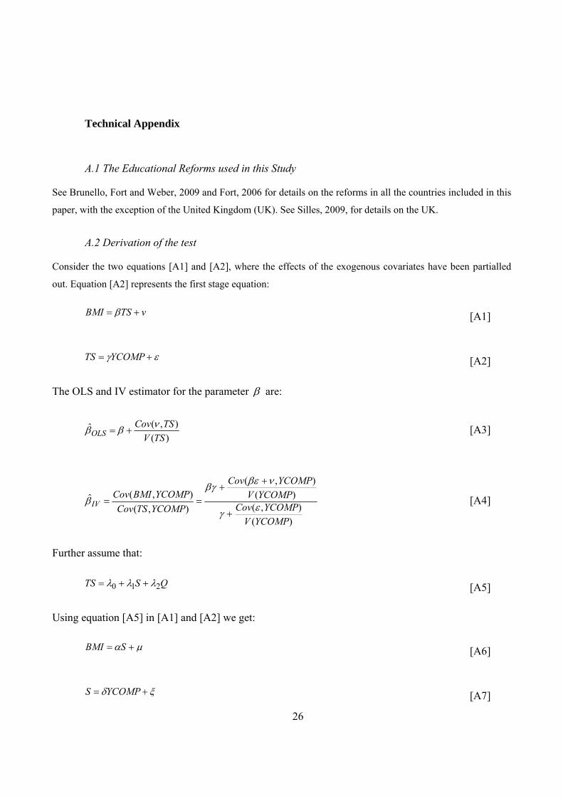
A.2 Derivation of the test

Consider the two equations [A1] and [A2], where the effects of the exogenous covariates have been partialled

out. Equation [A2] represents the first stage equation:

vTSBMI [A1]

YCOMPTS [A2]

The OLS and IV estimator for the parameter are:

)(

),(ˆTSV

TSCovOLS

[A3]

)(

),()(

),(

),(

),(ˆ

YCOMPV

YCOMPCovYCOMPV

YCOMPCov

YCOMPTSCov

YCOMPBMICovIV

[A4]

Further assume that:

QSTS 210 [A5]

Using equation [A5] in [A1] and [A2] we get:

SBMI [A6]

YCOMPS [A7]

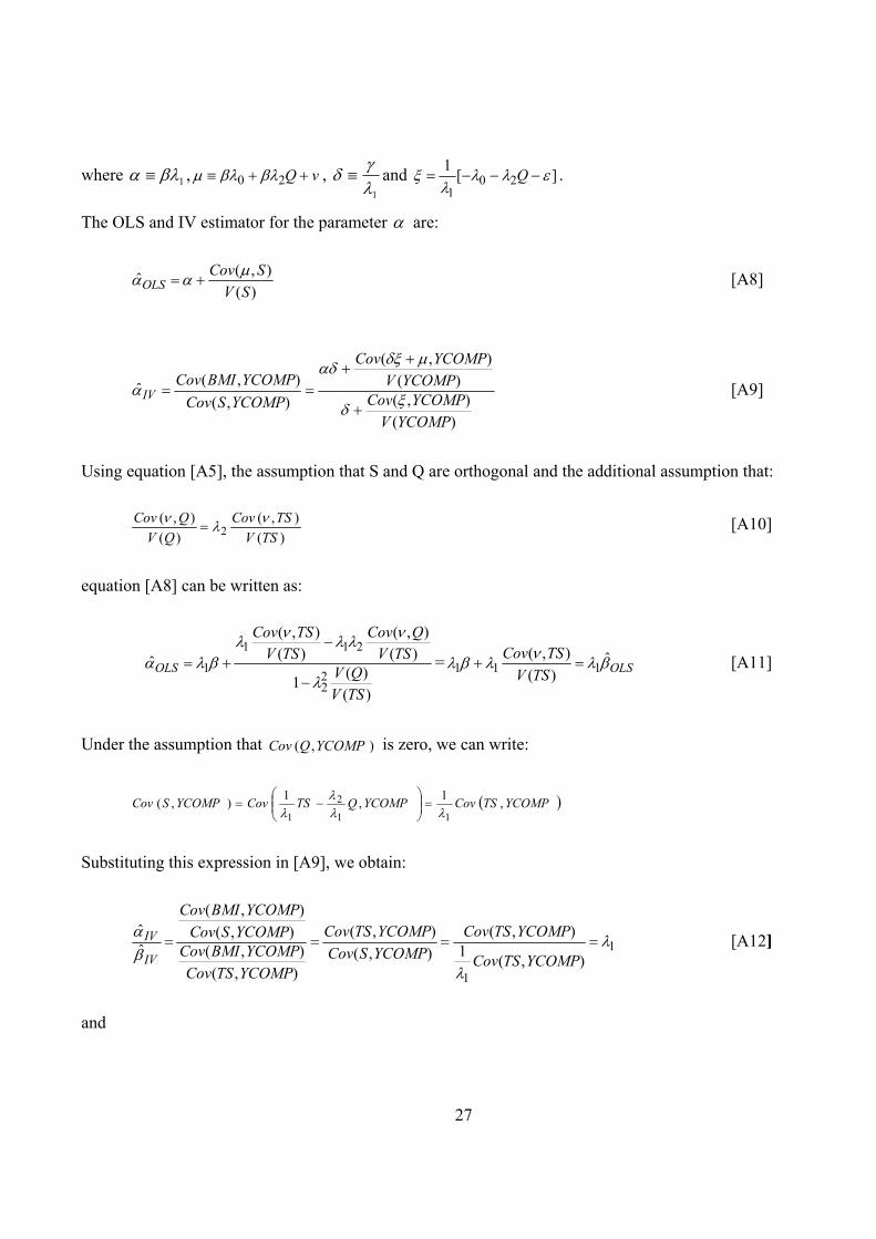
27

where 1 , vQ 20 , 1 and ][

120

1

Q .

The OLS and IV estimator for the parameter are:

)(

),(ˆSV

SCovOLS

[A8]

)(

),()(

),(

),(

),(ˆ

YCOMPV

YCOMPCovYCOMPV

YCOMPCov

YCOMPSCov

YCOMPBMICovIV

[A9]

Using equation [A5], the assumption that S and Q are orthogonal and the additional assumption that:

)(

),(

)(

),(2 TSV

TSCov

QV

QCov [A10]

equation [A8] can be written as:

)()(

1

)(),(

)(),(

ˆ22

211

1

TSVQV

TSVQCov

TSVTSCov

OLS

= OLSTSV

TSCov ˆ)(

),(111 [A11]

Under the assumption that ),( YCOMPQCov is zero, we can write:

YCOMPTSCovYCOMPQTSCovYCOMPSCov ,1

,1

),(11

2

1

Substituting this expression in [A9], we obtain:

1

1),(

1),(

),(

),(

),(

),(),(

),(

ˆˆ

YCOMPTSCov

YCOMPTSCov

YCOMPSCov

YCOMPTSCov

YCOMPTSCov

YCOMPBMICovYCOMPSCov

YCOMPBMICov

IV

IV [A12]

and

28

OLS

OLS

IV

IV

ˆˆ

ˆˆ

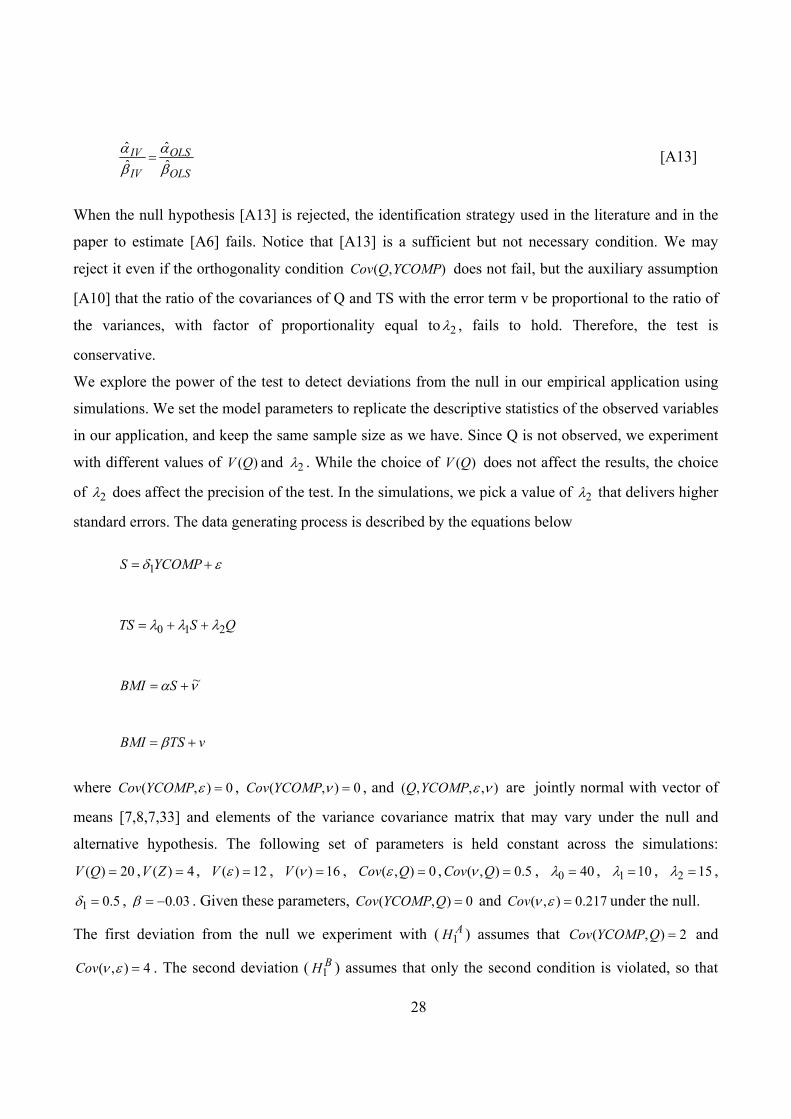
[A13]

When the null hypothesis [A13] is rejected, the identification strategy used in the literature and in the

paper to estimate [A6] fails. Notice that [A13] is a sufficient but not necessary condition. We may

reject it even if the orthogonality condition ),( YCOMPQCov does not fail, but the auxiliary assumption

[A10] that the ratio of the covariances of Q and TS with the error term v be proportional to the ratio of

the variances, with factor of proportionality equal to 2 , fails to hold. Therefore, the test is

conservative.

We explore the power of the test to detect deviations from the null in our empirical application using

simulations. We set the model parameters to replicate the descriptive statistics of the observed variables

in our application, and keep the same sample size as we have. Since Q is not observed, we experiment

with different values of )(QV and 2 . While the choice of )(QV does not affect the results, the choice

of 2 does affect the precision of the test. In the simulations, we pick a value of 2 that delivers higher

standard errors. The data generating process is described by the equations below

YCOMPS 1

QSTS 210

~ SBMI

vTSBMI

where 0),( YCOMPCov , 0),( YCOMPCov , and ),,,( YCOMPQ are jointly normal with vector of

means [7,8,7,33] and elements of the variance covariance matrix that may vary under the null and

alternative hypothesis. The following set of parameters is held constant across the simulations:

20)( QV , 4)( ZV , 12)( V , 16)( V , 0),( QCov , 5.0),( QCov , 400 , 101 , 152 ,

5.01 , 03.0 . Given these parameters, 0),( QYCOMPCov and 217.0),( Cov under the null.

The first deviation from the null we experiment with ( AH1 ) assumes that 2),( QYCOMPCov and

4),( Cov . The second deviation ( BH1 ) assumes that only the second condition is violated, so that

29

0),( QYCOMPCov and 4),( Cov . The third deviation ( CH1 ) assumes that only the first condition is

violated, so that 2),( QYCOMPCov and 217.0),( Cov . Table A3 summarizes the results of the

simulations. The empirical distribution of the test under each alternative hypothesis is reported in

Figure A2. The test turns out to be able to discriminate the null from each alternative hypothesis.

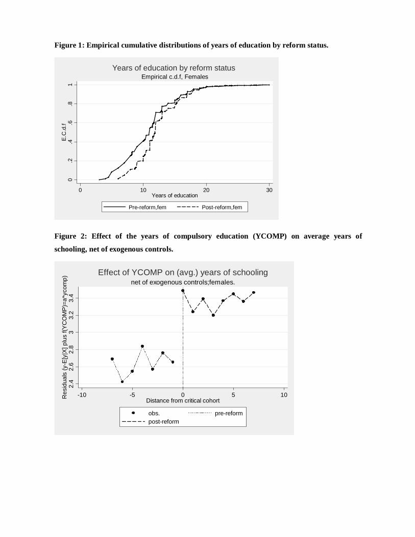
Figure 1: Empirical cumulative distributions of years of education by reform status.

0.2

.4.6

.81

E.C

.d.f

0 10 20 30Years of education

Pre-reform,fem Post-reform,fem

Empirical c.d.f, FemalesYears of education by reform status

Figure 2: Effect of the years of compulsory education (YCOMP) on average years of

schooling, net of exogenous controls.

2.4

2.6

2.8

33.

23.

4R

esid

uals

(y-

E[y

|X] p

lus

f(Y

CO

MP

)=a*

ycom

p)

-10 -5 0 5 10Distance from critical cohort

obs. pre-reformpost-reform

net of exogenous controls;females.Effect of YCOMP on (avg.) years of schooling

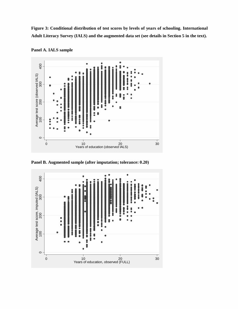
Figure 3: Conditional distribution of test scores by levels of years of schooling. International

Adult Literacy Survey (IALS) and the augmented data set (see details in Section 5 in the text).

Panel A. IALS sample

010

020

030

040

0A

vera

ge te

st s

core

(ob

serv

ed IA

LS)

0 10 20 30Years of education (observed IALS)

Panel B. Augmented sample (after imputation; tolerance: 0.20)

010

020

030

040

0A

vera

ge te

st s

core

, im

pute

d (I

ALS

)

0 10 20 30Years of education, observed (FULL)

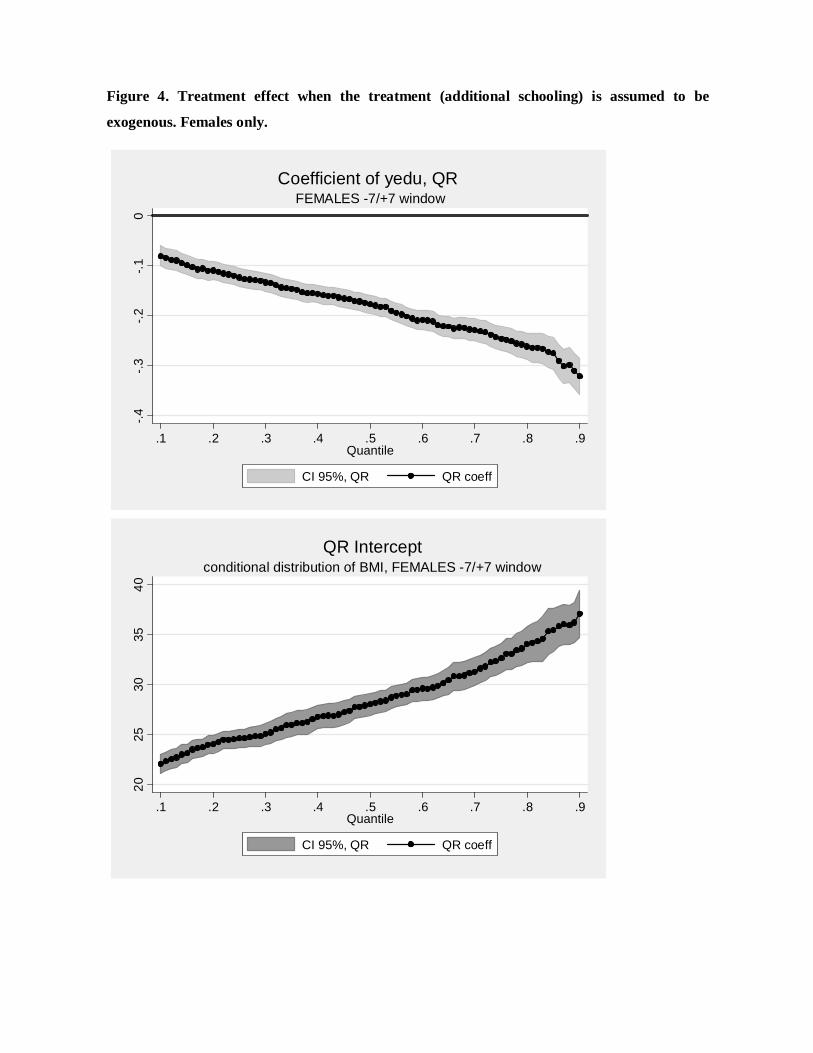
Figure 4. Treatment effect when the treatment (additional schooling) is assumed to be

exogenous. Females only. -.

4-.

3-.

2-.

10

.1 .2 .3 .4 .5 .6 .7 .8 .9Quantile

CI 95%, QR QR coeff

FEMALES -7/+7 windowCoefficient of yedu, QR

20

2530

354

0

.1 .2 .3 .4 .5 .6 .7 .8 .9Quantile

CI 95%, QR QR coeff

conditional distribution of BMI, FEMALES -7/+7 window QR Intercept

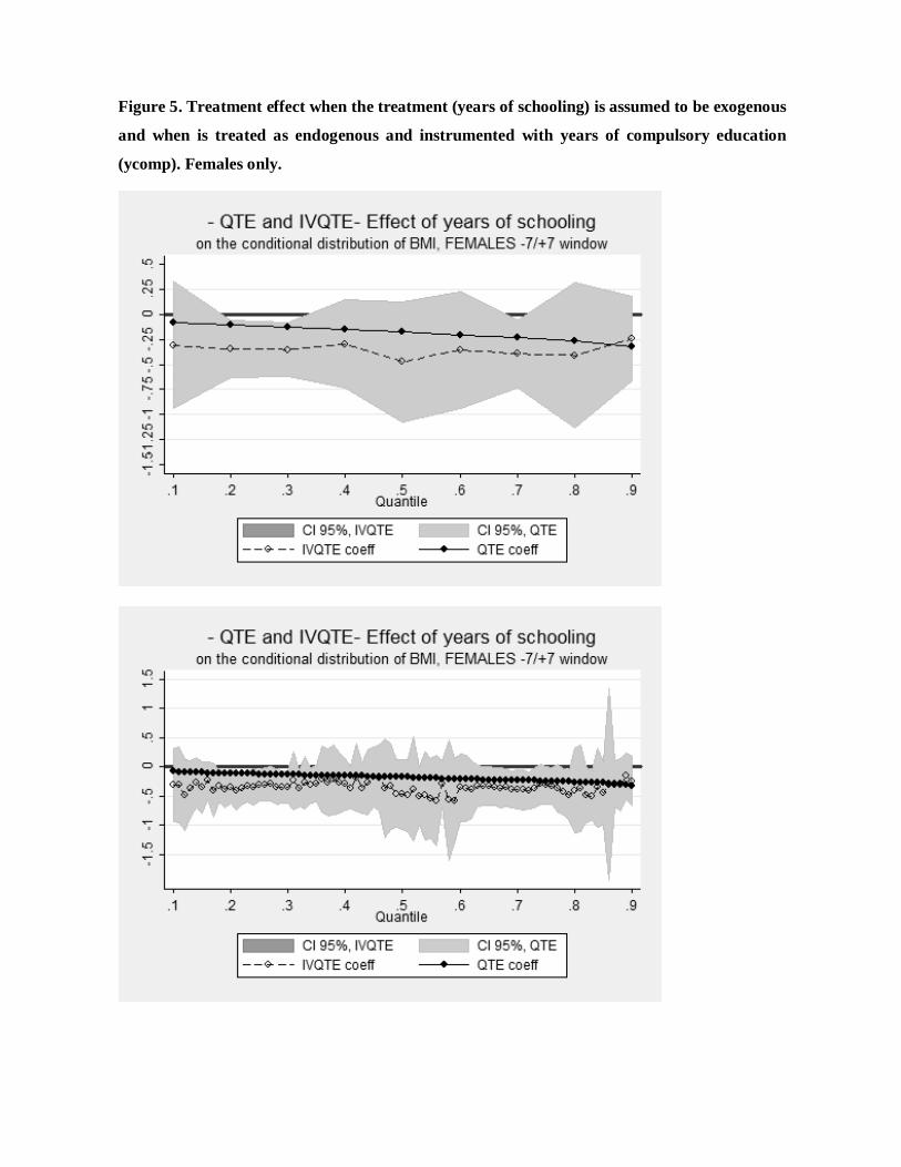
Figure 5. Treatment effect when the treatment (years of schooling) is assumed to be exogenous

and when is treated as endogenous and instrumented with years of compulsory education

(ycomp). Females only.

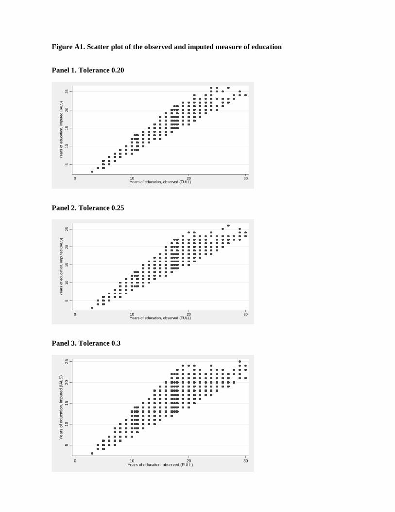
Figure A1. Scatter plot of the observed and imputed measure of education

Panel 1. Tolerance 0.20 5

1015

2025

Yea

rs o

f ed

ucat

ion,

impu

ted

(IA

LS)

0 10 20 30Years of education, observed (FULL)

Panel 2. Tolerance 0.25

510

1520

25

Yea

rs o

f ed

ucat

ion,

impu

ted

(IA

LS)

0 10 20 30Years of education, observed (FULL)

Panel 3. Tolerance 0.3

510

1520

25Y

ears

of e

duca

tion,

impu

ted

(IA

LS)

0 10 20 30Years of education, observed (FULL)

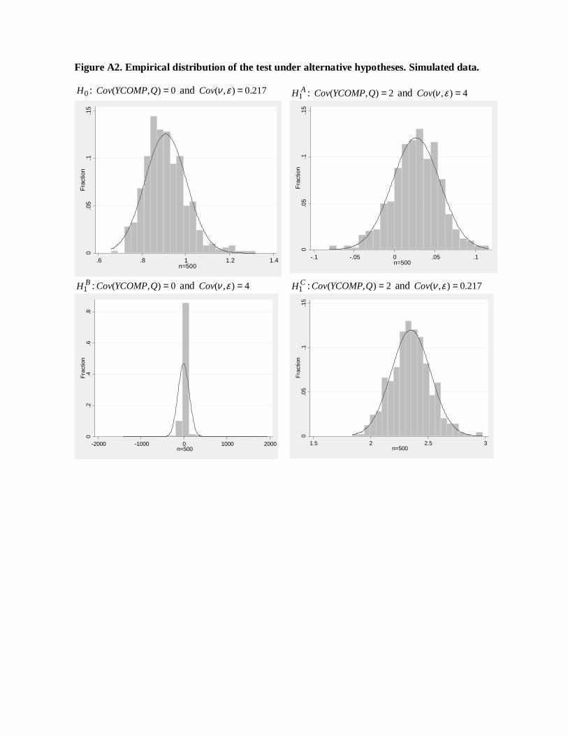
Figure A2. Empirical distribution of the test under alternative hypotheses. Simulated data.

0H : 0),( =QYCOMPCov and 217.0),( =ενCov AH1 : 2),( =QYCOMPCov and 4),( =ενCov 0

.05

.1.1

5F

ract

ion

.6 .8 1 1.2 1.4n=500

0.0

5.1

.15

Fra

ctio

n

-.1 -.05 0 .05 .1n=500

BH1 : 0),( =QYCOMPCov and 4),( =ενCov CH1 : 2),( =QYCOMPCov and 217.0),( =ενCov

0.2

.4.6

.8F

ract

ion

-2000 -1000 0 1000 2000n=500

0.0

5.1

.15

Fra

ctio

n

1.5 2 2.5 3n=500

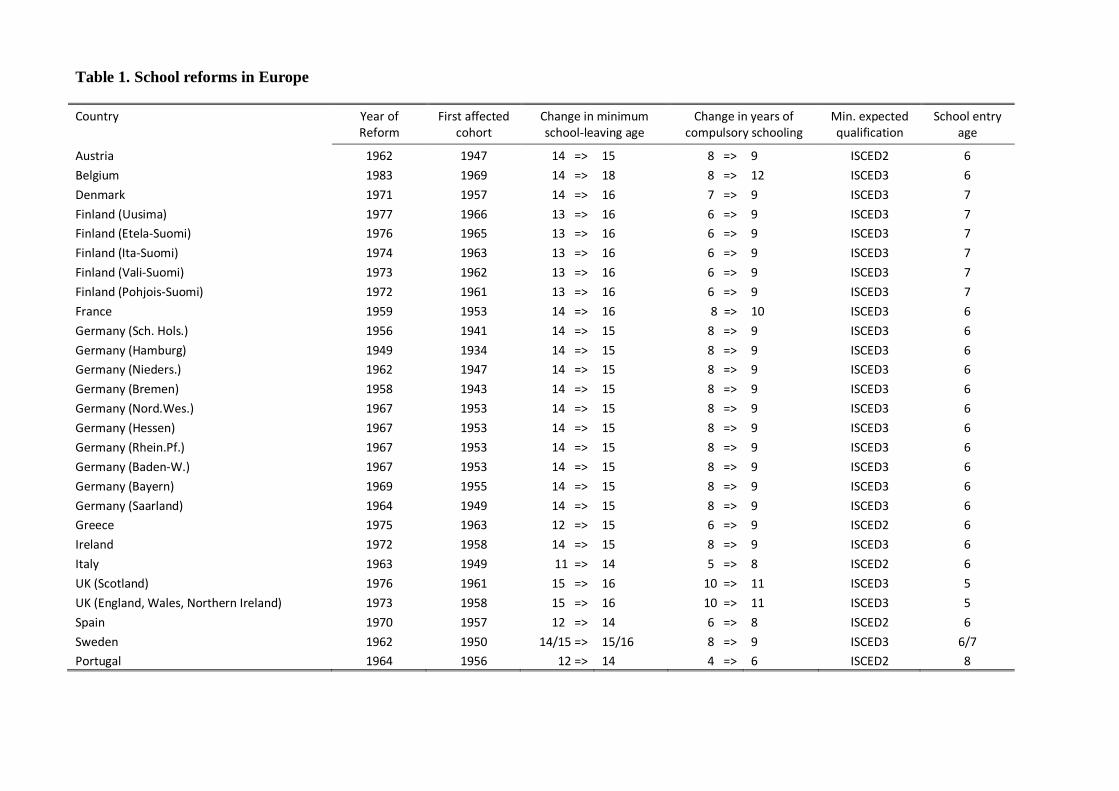
Table 1. School reforms in Europe

Country Year of Reform

First affected cohort

Change in minimum school-leaving age

Change in years of compulsory schooling

Min. expected qualification

School entry age

Austria 1962 1947 14 => 15 8 => 9 ISCED2 6

Belgium 1983 1969 14 => 18 8 => 12 ISCED3 6

Denmark 1971 1957 14 => 16 7 => 9 ISCED3 7

Finland (Uusima) 1977 1966 13 => 16 6 => 9 ISCED3 7

Finland (Etela-Suomi) 1976 1965 13 => 16 6 => 9 ISCED3 7

Finland (Ita-Suomi) 1974 1963 13 => 16 6 => 9 ISCED3 7

Finland (Vali-Suomi) 1973 1962 13 => 16 6 => 9 ISCED3 7

Finland (Pohjois-Suomi) 1972 1961 13 => 16 6 => 9 ISCED3 7

France 1959 1953 14 => 16 8 => 10 ISCED3 6

Germany (Sch. Hols.) 1956 1941 14 => 15 8 => 9 ISCED3 6

Germany (Hamburg) 1949 1934 14 => 15 8 => 9 ISCED3 6

Germany (Nieders.) 1962 1947 14 => 15 8 => 9 ISCED3 6

Germany (Bremen) 1958 1943 14 => 15 8 => 9 ISCED3 6

Germany (Nord.Wes.) 1967 1953 14 => 15 8 => 9 ISCED3 6

Germany (Hessen) 1967 1953 14 => 15 8 => 9 ISCED3 6

Germany (Rhein.Pf.) 1967 1953 14 => 15 8 => 9 ISCED3 6

Germany (Baden-W.) 1967 1953 14 => 15 8 => 9 ISCED3 6

Germany (Bayern) 1969 1955 14 => 15 8 => 9 ISCED3 6

Germany (Saarland) 1964 1949 14 => 15 8 => 9 ISCED3 6

Greece 1975 1963 12 => 15 6 => 9 ISCED2 6

Ireland 1972 1958 14 => 15 8 => 9 ISCED3 6

Italy 1963 1949 11 => 14 5 => 8 ISCED2 6

UK (Scotland) 1976 1961 15 => 16 10 => 11 ISCED3 5

UK (England, Wales, Northern Ireland) 1973 1958 15 => 16 10 => 11 ISCED3 5

Spain 1970 1957 12 => 14 6 => 8 ISCED2 6

Sweden 1962 1950 14/15 => 15/16 8 => 9 ISCED3 6/7

Portugal 1964 1956 12 => 14 4 => 6 ISCED2 8

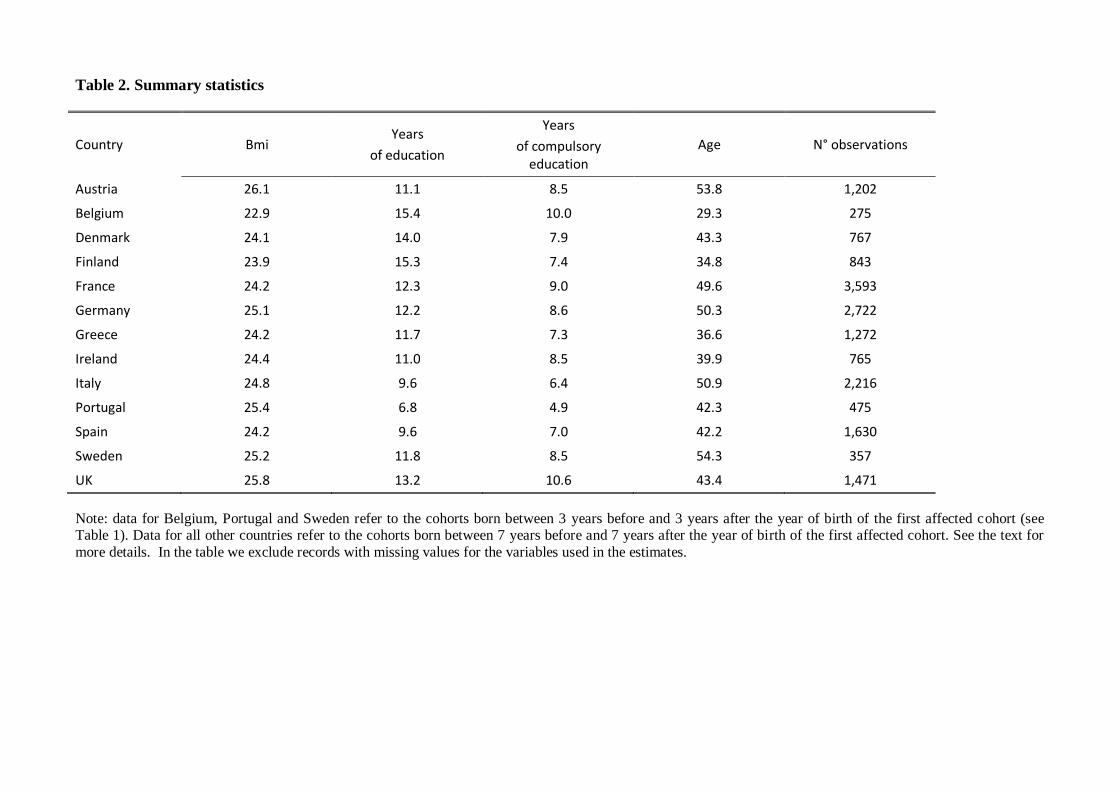
Table 2. Summary statistics

Country Bmi Years

of education

Years

of compulsory education

Age N° observations

Austria 26.1 11.1 8.5 53.8 1,202

Belgium 22.9 15.4 10.0 29.3 275

Denmark 24.1 14.0 7.9 43.3 767

Finland 23.9 15.3 7.4 34.8 843

France 24.2 12.3 9.0 49.6 3,593

Germany 25.1 12.2 8.6 50.3 2,722

Greece 24.2 11.7 7.3 36.6 1,272

Ireland 24.4 11.0 8.5 39.9 765

Italy 24.8 9.6 6.4 50.9 2,216

Portugal 25.4 6.8 4.9 42.3 475

Spain 24.2 9.6 7.0 42.2 1,630

Sweden 25.2 11.8 8.5 54.3 357

UK 25.8 13.2 10.6 43.4 1,471

Note: data for Belgium, Portugal and Sweden refer to the cohorts born between 3 years before and 3 years after the year of birth of the first affected cohort (see Table 1). Data for all other countries refer to the cohorts born between 7 years before and 7 years after the year of birth of the first affected cohort. See the text for

more details. In the table we exclude records with missing values for the variables used in the estimates.

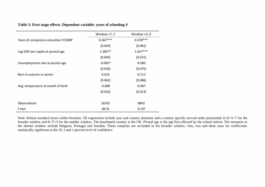
Table 3: First stage effects. Dependent variable: years of schooling S

Window +7,-7 Window +3,-3

Years of compulsory education YCOMP 0.367*** 0.378***

[0.059] [0.081]

Log GDP per-capita at pivotal age 1.385** 1.627***

[0.604] [0.615]

Unemployment rate at pivotal age -0.065* -0.082

[0.039] [0.075]

Born in autumn or winter 0.016 -0.111

[0.063] [0.086]

Avg. temperature at month of birth -0.008 -0.007

[0.010] [0.013]

Observations 16335 8843

F test 38.35 21.87

Note: Robust standard errors within brackets. All regressions include year and country dummies and a country specific second order polynomial in K=T+7 for the broader window and K=T+3 for the smaller window. The benchmark country is the UK. Pivotal age is the age first affected by the school reform. The estimates in

the shorter window include Belgium, Portugal and Sweden. These countries are excluded in the broader window. One, two and three stars for coefficients

statistically significant at the 10, 5 and 1 percent level of confidence.

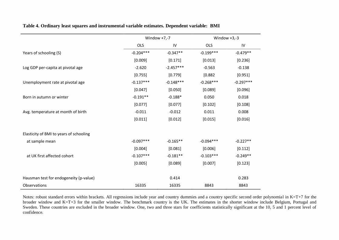
Table 4. Ordinary least squares and instrumental variable estimates. Dependent variable: BMI

Window +7,-7 Window +3,-3

OLS IV OLS IV

Years of schooling (S) -0.204*** -0.347** -0.199*** -0.479**

[0.009] [0.171] [0.013] [0.236]

Log GDP per-capita at pivotal age -2.620 -2.457*** -0.563 -0.138

[0.755] [0.779] [0.882 [0.951]

Unemployment rate at pivotal age -0.137*** -0.148*** -0.268*** -0.297***

[0.047] [0.050] [0.089] [0.096]

Born in autumn or winter -0.191** -0.188* 0.050 0.018

[0.077] [0.077] [0.102] [0.108]

Avg. temperature at month of birth -0.011 -0.012 0.011 0.008

[0.011] [0.012] [0.015] [0.016]

Elasticity of BMI to years of schooling

at sample mean -0.097*** -0.165** -0.094*** -0.227**

[0.004] [0.081] [0.006] [0.112]

at UK first affected cohort -0.107*** -0.181** -0.103*** -0.249**

[0.005] [0.089] [0.007] [0.123]

Hausman test for endogeneity (p-value) 0.414 0.283

Observations 16335 16335 8843 8843

Notes: robust standard errors within brackets. All regressions include year and country dummies and a country specific second order polynomial in K=T+7 for the

broader window and K=T+3 for the smaller window. The benchmark country is the UK. The estimates in the shorter window include Belgium, Portugal and

Sweden. These countries are excluded in the broader window. One, two and three stars for coefficients statistically significant at the 10, 5 and 1 percent level of

confidence.

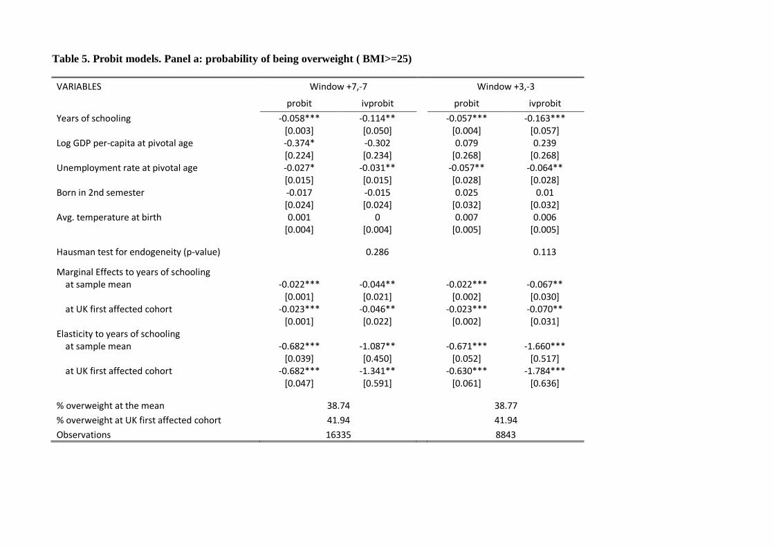
Table 5. Probit models. Panel a: probability of being overweight ( BMI>=25)

VARIABLES Window +7,-7 Window +3,-3

probit ivprobit probit ivprobit

Years of schooling -0.058*** -0.114** -0.057*** -0.163*** [0.003] [0.050] [0.004] [0.057] Log GDP per-capita at pivotal age -0.374* -0.302 0.079 0.239 [0.224] [0.234] [0.268] [0.268] Unemployment rate at pivotal age -0.027* -0.031** -0.057** -0.064** [0.015] [0.015] [0.028] [0.028] Born in 2nd semester -0.017 -0.015 0.025 0.01 [0.024] [0.024] [0.032] [0.032] Avg. temperature at birth 0.001 0 0.007 0.006 [0.004] [0.004] [0.005] [0.005]

Hausman test for endogeneity (p-value) 0.286 0.113

Marginal Effects to years of schooling at sample mean -0.022*** -0.044** -0.022*** -0.067** [0.001] [0.021] [0.002] [0.030] at UK first affected cohort -0.023*** -0.046** -0.023*** -0.070** [0.001] [0.022] [0.002] [0.031] Elasticity to years of schooling at sample mean -0.682*** -1.087** -0.671*** -1.660*** [0.039] [0.450] [0.052] [0.517] at UK first affected cohort -0.682*** -1.341** -0.630*** -1.784*** [0.047] [0.591] [0.061] [0.636]

% overweight at the mean 38.74 38.77

% overweight at UK first affected cohort 41.94 41.94

Observations 16335 8843

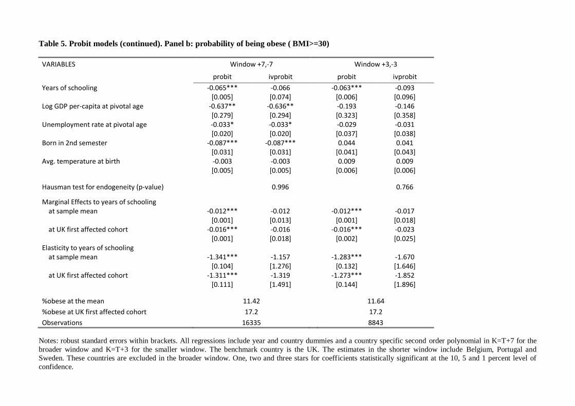
Table 5. Probit models (continued). Panel b: probability of being obese ( BMI>=30)

VARIABLES Window +7,-7 Window +3,-3

probit ivprobit probit ivprobit

Years of schooling -0.065*** -0.066 -0.063*** -0.093 [0.005] [0.074] [0.006] [0.096] Log GDP per-capita at pivotal age -0.637** -0.636** -0.193 -0.146 [0.279] [0.294] [0.323] [0.358] Unemployment rate at pivotal age -0.033* -0.033* -0.029 -0.031 [0.020] [0.020] [0.037] [0.038] Born in 2nd semester -0.087*** -0.087*** 0.044 0.041 [0.031] [0.031] [0.041] [0.043] Avg. temperature at birth -0.003 -0.003 0.009 0.009 [0.005] [0.005] [0.006] [0.006]

Hausman test for endogeneity (p-value) 0.996 0.766

Marginal Effects to years of schooling at sample mean -0.012*** -0.012 -0.012*** -0.017 [0.001] [0.013] [0.001] [0.018] at UK first affected cohort -0.016*** -0.016 -0.016*** -0.023 [0.001] [0.018] [0.002] [0.025] Elasticity to years of schooling at sample mean -1.341*** -1.157 -1.283*** -1.670 [0.104] [1.276] [0.132] [1.646] at UK first affected cohort -1.311*** -1.319 -1.273*** -1.852 [0.111] [1.491] [0.144] [1.896]

%obese at the mean 11.42 11.64

%obese at UK first affected cohort 17.2 17.2

Observations 16335 8843

Notes: robust standard errors within brackets. All regressions include year and country dummies and a country specific second order polynomial in K=T+7 for the

broader window and K=T+3 for the smaller window. The benchmark country is the UK. The estimates in the shorter window include Belgium, Portugal and

Sweden. These countries are excluded in the broader window. One, two and three stars for coefficients statistically significant at the 10, 5 and 1 percent level of

confidence.

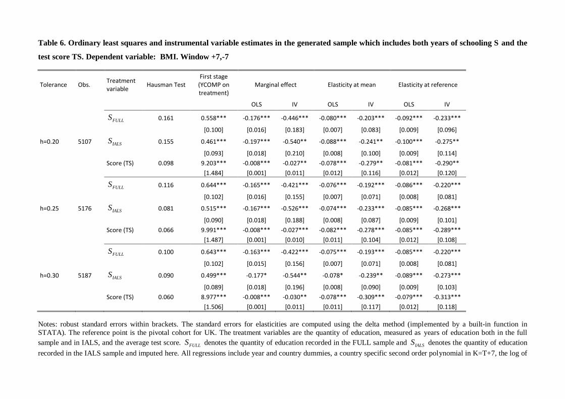
Table 6. Ordinary least squares and instrumental variable estimates in the generated sample which includes both years of schooling S and the

test score TS. Dependent variable: BMI. Window +7,-7

Tolerance Obs. Treatment variable

Hausman Test First stage

(YCOMP on treatment)

Marginal effect Elasticity at mean Elasticity at reference

OLS IV OLS IV OLS IV

FULLS 0.161 0.558*** -0.176*** -0.446*** -0.080*** -0.203*** -0.092*** -0.233***

[0.100] [0.016] [0.183] [0.007] [0.083] [0.009] [0.096]

h=0.20 5107 IALSS 0.155 0.461*** -0.197*** -0.540** -0.088*** -0.241** -0.100*** -0.275**

[0.093] [0.018] [0.210] [0.008] [0.100] [0.009] [0.114]

Score (TS) 0.098 9.203*** -0.008*** -0.027** -0.078*** -0.279** -0.081*** -0.290**

[1.484] [0.001] [0.011] [0.012] [0.116] [0.012] [0.120]

FULLS 0.116 0.644*** -0.165*** -0.421*** -0.076*** -0.192*** -0.086*** -0.220***

[0.102] [0.016] [0.155] [0.007] [0.071] [0.008] [0.081]

h=0.25 5176 IALSS 0.081 0.515*** -0.167*** -0.526*** -0.074*** -0.233*** -0.085*** -0.268***

[0.090] [0.018] [0.188] [0.008] [0.087] [0.009] [0.101]

Score (TS) 0.066 9.991*** -0.008*** -0.027*** -0.082*** -0.278*** -0.085*** -0.289***

[1.487] [0.001] [0.010] [0.011] [0.104] [0.012] [0.108]

FULLS 0.100 0.643*** -0.163*** -0.422*** -0.075*** -0.193*** -0.085*** -0.220***

[0.102] [0.015] [0.156] [0.007] [0.071] [0.008] [0.081]

h=0.30 5187 IALSS 0.090 0.499*** -0.177* -0.544** -0.078* -0.239** -0.089*** -0.273***

[0.089] [0.018] [0.196] [0.008] [0.090] [0.009] [0.103]

Score (TS) 0.060 8.977*** -0.008*** -0.030** -0.078*** -0.309*** -0.079*** -0.313***

[1.506] [0.001] [0.011] [0.011] [0.117] [0.012] [0.118]

Notes: robust standard errors within brackets. The standard errors for elasticities are computed using the delta method (implemented by a built-in function in STATA). The reference point is the pivotal cohort for UK. The treatment variables are the quantity of education, measured as years of education both in the full

sample and in IALS, and the average test score. FULLS denotes the quantity of education recorded in the FULL sample and IALSS denotes the quantity of education

recorded in the IALS sample and imputed here. All regressions include year and country dummies, a country specific second order polynomial in K=T+7, the log of

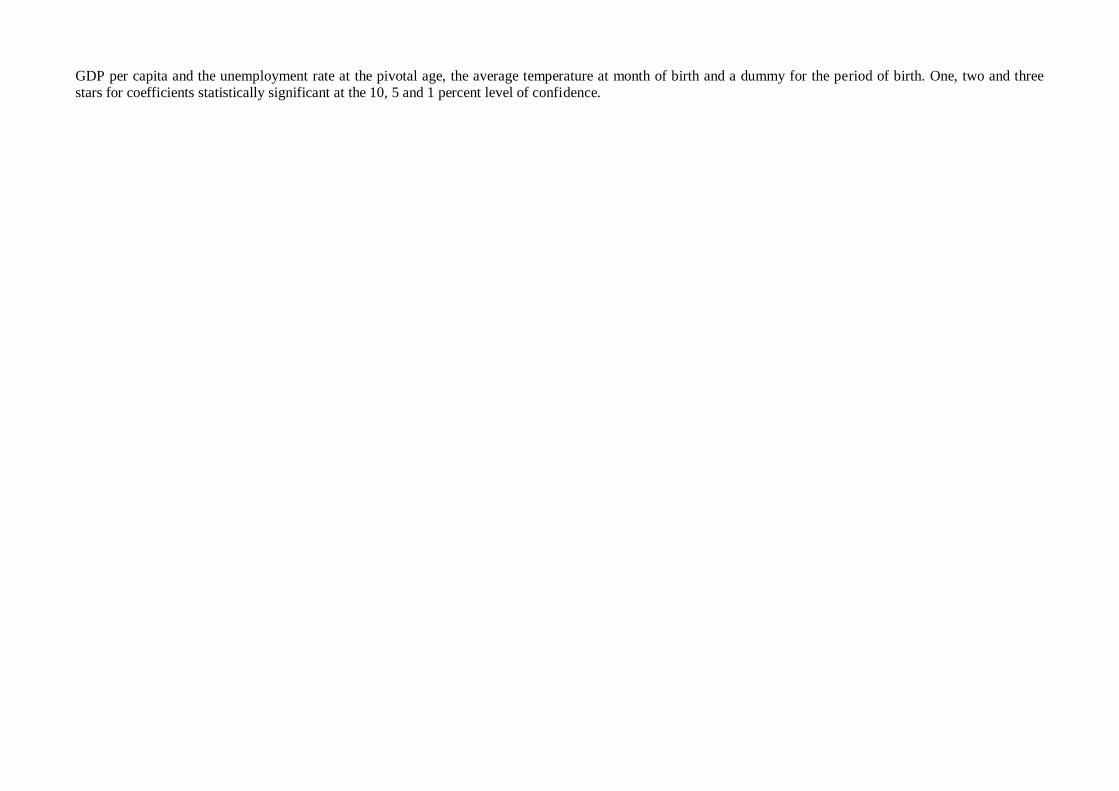
GDP per capita and the unemployment rate at the pivotal age, the average temperature at month of birth and a dummy for the period of birth. One, two and three stars for coefficients statistically significant at the 10, 5 and 1 percent level of confidence.

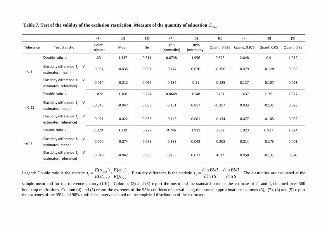
Table 7. Test of the validity of the exclusion restriction. Measure of the quantity of education IALSS

(1) (2) (3) (4) (5) (6) (7) (8) (9)

Tolerance Test statistic Point

estimate Mean Se

LB95 (normality)

UB95 (normality)

Quant. 0.025 Quant. 0.975 Quant. 0.05 Quant. 0.95

h=0.2

Double ratio 1t 1.231 1.347 0.311 0.0738 1.956 0.823 2.048 0.9 1.919

Elasticity difference 2t (IV

estimates, mean) -0.037 -0.035 0.057 -0.147 0.076 -0.156 0.079 -0.128 0.058

Elasticity difference 2t (IV

estimates, reference) -0.014 -0.012 0.062 -0.132 0.11 -0.125 0.127 -0.107 0.093

h=0.25

Double ratio 1t 1.072 1.108 0.224 0.0668 1.548 0.751 1.637 0.79 1.527

Elasticity difference 2t (IV

estimates, mean) -0.045 -0.047 0.053 -0.151 0.057 -0.157 0.033 -0.131 0.023

Elasticity difference 2t (IV

estimates, reference) -0.021 -0.022 0.053 -0.126 0.081 -0.134 0.077 -0.105 0.052

h=0.3

Double ratio 1t 1.220 1.329 0.297 0.746 1.911 0.882 1.923 0.927 1.824

Elasticity difference 2t (IV

estimates, mean) -0.070 -0.074 0.059 -0.188 0.042 -0.208 0.014 -0.173 0.001

Elasticity difference 2t (IV

estimates, reference) -0.040 -0.042 0.058 -0.155 0.072 -0.17 0.058 -0.131 0.04

Legend: Double ratio is the statistic 1

( ) ( )/

( ) ( )

OLS IV

OLS IV

E Et

E E

; Elasticity difference is the statistic 2

ln ln

ln ln

BMI BMIt

TS S

. The elasticities are evaluated at the

sample mean and for the reference country (UK). Columns (2) and (3) report the mean and the standard error of the estimate of 1t and 2t obtained over 500

bootstrap replications. Column (4) and (5) report the extremes of the 95% confidence interval using the normal approximation; columns (6), (7), (8) and (9) report

the extremes of the 95% and 90% confidence intervals based on the empirical distribution of the estimators.

FULLSFULLSIALSSFULLSIALSSFULLSIALSSFULLSIALSSFULLSIALSSIALSSFULLSIALSSFULLSIALSSFULLSIALSSFULLSIALSSFULLSIALSS

FULLSFULLSIALSSFULLSIALSSFULLSIALSSFULLSIALSSFULLSIALSSIALSSFULLSIALSSFULLSIALSSFULLSIALSSFULLSIALSSFULLSIALSS

FULLSFULLSIALSSFULLSIALSSFULLSIALSSFULLSIALSSFULLSIALSSIALSSFULLSIALSSFULLSIALSSFULLSIALSSFULLSIALSSFULLSIALSS

Table 8. Test of the validity of the exclusion restriction. Measure of the quantity of education FULLS

(1) (2) (3) (4) (5) (6) (7) (8) (9)

Tolerance Test statistic Point

estimate Mean Se

LB95 (normality)

UB95 (normality)

Quant. 0.025 Quant. 0.975 Quant. 0.05 Quant. 0.95

h=0.2

Double ratio 1t 1.332 1.472 0.341 0.804 2.14 0.0927 2.298 0.98 2.081

Elasticity difference 2t

(IV estimates, mean) -0.076* -0.076 0.056 -0.187 0.034 -0.21 0.0196 -0.178 -0.001

Elasticity difference 2t

(IV estimates, reference) -0.056 -0.057 0.057 -0.168 0.055 -0.184 0.043 -0.16 0.021

h=0.25

Double ratio 1t 1.323 1.373 0.291 0.082 1.943 0.911 1.994 0.955 1.914

Elasticity difference 2t

(IV estimates, mean) -0.086** -0.09 0.06 -0.207 0.027 -0.222 -0.005 -0.191 -0.014

Elasticity difference 2t

(IV estimates, reference) -0.069 -0.074 0.058 -0.187 0.04 -0.21 0.011 -0.175 0

h=0.3

Double ratio 1t 1.448** 1.6 0.396 0.824 2.376 1.022 2.433 1.089 2.243

Elasticity difference 2t

(IV estimates, mean) -0.116** -0.121 0.067 -0.251 0.009 -0.275 -0.022 -0.239 -0.033

Elasticity difference 2t

(IV estimates, reference) -0.093** -0.097 0.064 -0.223 0.028 -0.237 -0.002 -0.197 -0.014

Legend: see Table 8.

FULLSFULLSIALSSFULLSIALSSFULLSIALSSFULLSIALSSFULLSIALSSIALSSFULLSIALSSFULLSIALSSFULLSIALSSFULLSIALSSFULLSIALSS

FULLSFULLSIALSSFULLSIALSSFULLSIALSSFULLSIALSSFULLSIALSSIALSSFULLSIALSSFULLSIALSSFULLSIALSSFULLSIALSSFULLSIALSS

FULLSFULLSIALSSFULLSIALSSFULLSIALSSFULLSIALSSFULLSIALSSIALSSFULLSIALSSFULLSIALSSFULLSIALSSFULLSIALSSFULLSIALSS

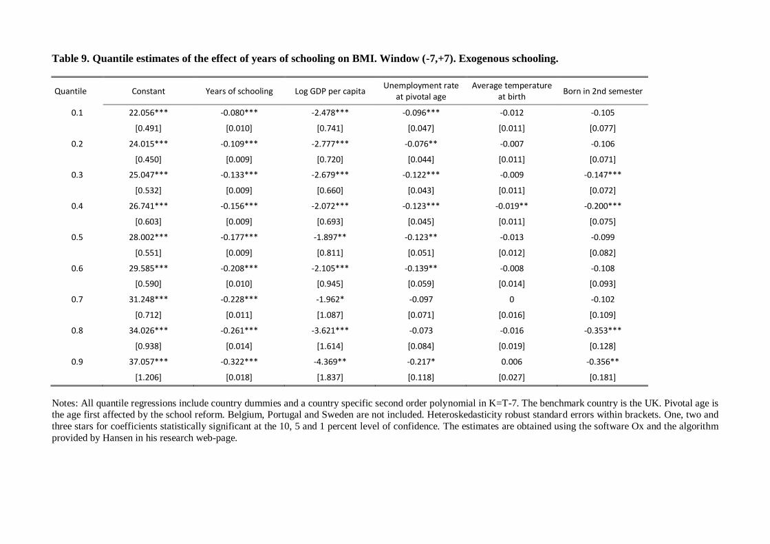
Table 9. Quantile estimates of the effect of years of schooling on BMI. Window (-7,+7). Exogenous schooling.

Quantile Constant Years of schooling Log GDP per capita Unemployment rate

at pivotal age Average temperature

at birth Born in 2nd semester

0.1 22.056*** -0.080*** -2.478*** -0.096*** -0.012 -0.105

[0.491] [0.010] [0.741] [0.047] [0.011] [0.077]

0.2 24.015*** -0.109*** -2.777*** -0.076** -0.007 -0.106

[0.450] [0.009] [0.720] [0.044] [0.011] [0.071]

0.3 25.047*** -0.133*** -2.679*** -0.122*** -0.009 -0.147***

[0.532] [0.009] [0.660] [0.043] [0.011] [0.072]

0.4 26.741*** -0.156*** -2.072*** -0.123*** -0.019** -0.200***

[0.603] [0.009] [0.693] [0.045] [0.011] [0.075]

0.5 28.002*** -0.177*** -1.897** -0.123** -0.013 -0.099

[0.551] [0.009] [0.811] [0.051] [0.012] [0.082]

0.6 29.585*** -0.208*** -2.105*** -0.139** -0.008 -0.108

[0.590] [0.010] [0.945] [0.059] [0.014] [0.093]

0.7 31.248*** -0.228*** -1.962* -0.097 0 -0.102

[0.712] [0.011] [1.087] [0.071] [0.016] [0.109]

0.8 34.026*** -0.261*** -3.621*** -0.073 -0.016 -0.353***

[0.938] [0.014] [1.614] [0.084] [0.019] [0.128]

0.9 37.057*** -0.322*** -4.369** -0.217* 0.006 -0.356**

[1.206] [0.018] [1.837] [0.118] [0.027] [0.181]

Notes: All quantile regressions include country dummies and a country specific second order polynomial in K=T-7. The benchmark country is the UK. Pivotal age is the age first affected by the school reform. Belgium, Portugal and Sweden are not included. Heteroskedasticity robust standard errors within brackets. One, two and

three stars for coefficients statistically significant at the 10, 5 and 1 percent level of confidence. The estimates are obtained using the software Ox and the algorithm

provided by Hansen in his research web-page.

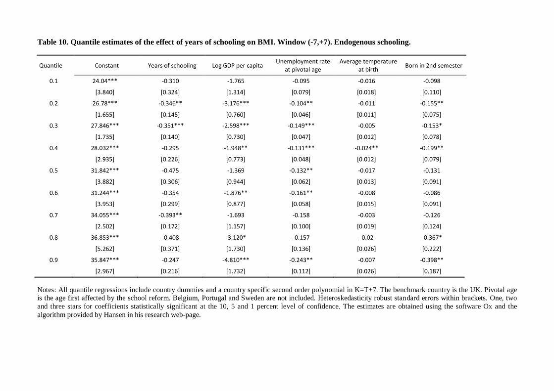
Table 10. Quantile estimates of the effect of years of schooling on BMI. Window (-7,+7). Endogenous schooling.

Quantile Constant Years of schooling Log GDP per capita Unemployment rate

at pivotal age Average temperature

at birth Born in 2nd semester

0.1 24.04*** -0.310 -1.765 -0.095 -0.016 -0.098

[3.840] [0.324] [1.314] [0.079] [0.018] [0.110]

0.2 26.78*** -0.346** -3.176*** -0.104** -0.011 -0.155**

[1.655] [0.145] [0.760] [0.046] [0.011] [0.075]

0.3 27.846*** -0.351*** -2.598*** -0.149*** -0.005 -0.153*

[1.735] [0.140] [0.730] [0.047] [0.012] [0.078]

0.4 28.032*** -0.295 -1.948** -0.131*** -0.024** -0.199**

[2.935] [0.226] [0.773] [0.048] [0.012] [0.079]

0.5 31.842*** -0.475 -1.369 -0.132** -0.017 -0.131

[3.882] [0.306] [0.944] [0.062] [0.013] [0.091]

0.6 31.244*** -0.354 -1.876** -0.161** -0.008 -0.086

[3.953] [0.299] [0.877] [0.058] [0.015] [0.091]

0.7 34.055*** -0.393** -1.693 -0.158 -0.003 -0.126

[2.502] [0.172] [1.157] [0.100] [0.019] [0.124]

0.8 36.853*** -0.408 -3.120* -0.157 -0.02 -0.367*

[5.262] [0.371] [1.730] [0.136] [0.026] [0.222]

0.9 35.847*** -0.247 -4.810*** -0.243** -0.007 -0.398**

[2.967] [0.216] [1.732] [0.112] [0.026] [0.187]

Notes: All quantile regressions include country dummies and a country specific second order polynomial in K=T+7. The benchmark country is the UK. Pivotal age is the age first affected by the school reform. Belgium, Portugal and Sweden are not included. Heteroskedasticity robust standard errors within brackets. One, two

and three stars for coefficients statistically significant at the 10, 5 and 1 percent level of confidence. The estimates are obtained using the software Ox and the

algorithm provided by Hansen in his research web-page.

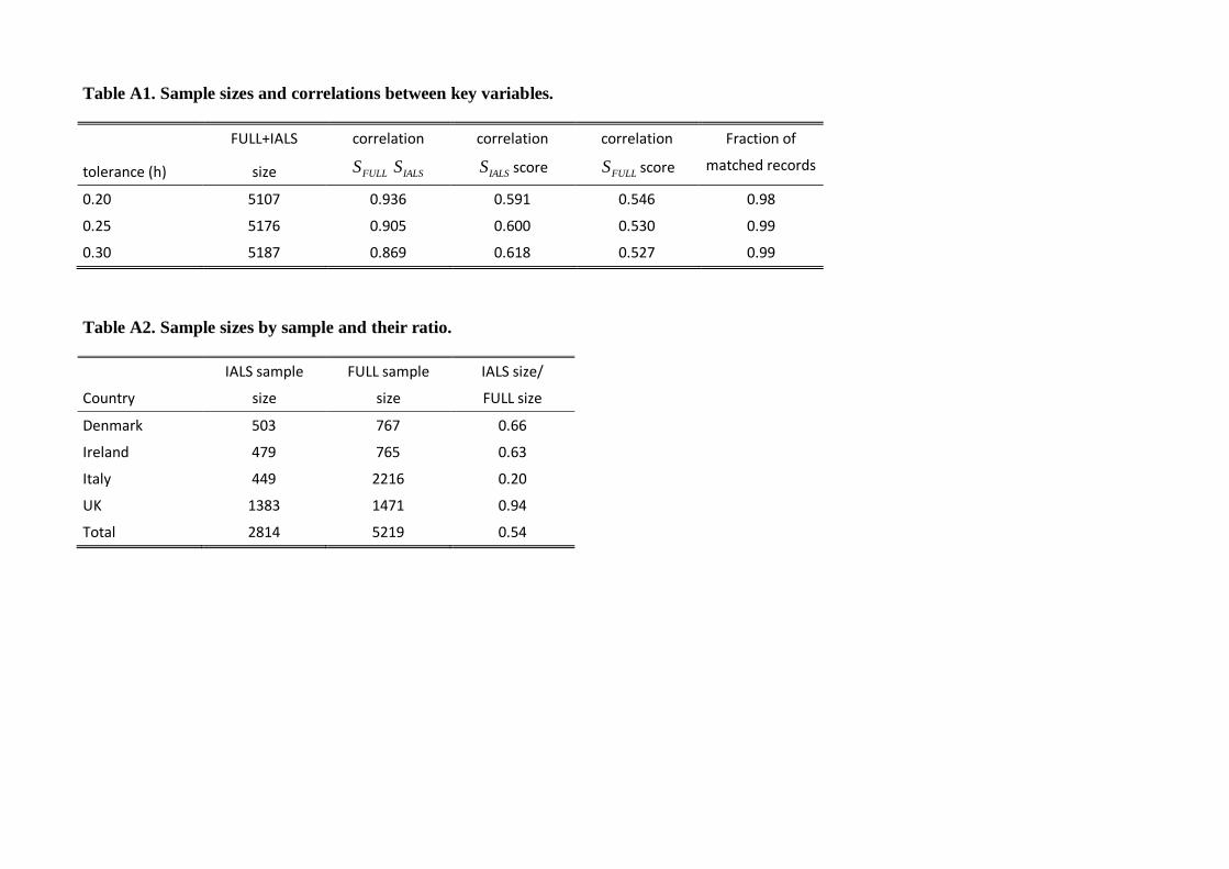
Table A1. Sample sizes and correlations between key variables.

FULL+IALS correlation correlation correlation Fraction of

tolerance (h) size FULLS IALSS IALSS score FULLS score matched records

0.20 5107 0.936 0.591 0.546 0.98

0.25 5176 0.905 0.600 0.530 0.99

0.30 5187 0.869 0.618 0.527 0.99

Table A2. Sample sizes by sample and their ratio.

IALS sample FULL sample IALS size/

Country size size FULL size

Denmark 503 767 0.66

Ireland 479 765 0.63

Italy 449 2216 0.20

UK 1383 1471 0.94

Total 2814 5219 0.54

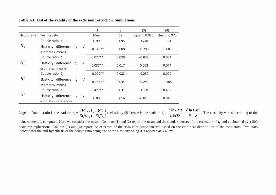
Table A3. Test of the validity of the exclusion restriction. Simulations.

(1) (2) (3) (4)

Hypothesis Test statistic Mean Se Quant. 0.025 Quant. 0.975

0H

Double ratio 1t 0.908 0.095 0.748 1.121

Elasticity difference 2t (IV

estimates, mean) -0.142** 0.008 -0.206 -0.081

1

AH

Double ratio 1t 0.027** 0.029 -0.036 0.084

Elasticity difference 2t (IV

estimates, mean) 0.037** 0.017 0.008 0.074

1

BH

Double ratio 1t -0.079** 0.082 -0.252 0.079

Elasticity difference 2t (IV

estimates, mean) -0.167** 0.034 -0.244 -0.105

1

CH

Double ratio 1t 0.427** 0.031 0.368 0.492

Elasticity difference 2t (IV

estimates, reference) 0.008 0.016 -0.023 0.040

Legend: Double ratio is the statistic 1

( ) ( )/

( ) ( )

OLS IV

OLS IV

E Et

E E

; elasticity difference is the statistic 2

ln ln

ln ln

BMI BMIt

TS S

. The elasticity varies according to the

point where it is computed. Here we consider the mean. Columns (1) and (2) report the mean and the standard errors of the estimator of 1t and 2t obtained over 500

bootstrap replications. Column (3) and (4) report the extremes of the 95% confidence interval based on the empirical distribution of the estimators. Two stars indicate that the null hypothesis of the double ratio being one or the elasticity being 0 is rejected at 5% level.

FULLSFULLSIALSSFULLSIALSSFULLSIALSSFULLSIALSSFULLSIALSSIALSSFULLSIALSSFULLSIALSSFULLSIALSSFULLSIALSSFULLSIALSS

FULLSFULLSIALSSFULLSIALSSFULLSIALSSFULLSIALSSFULLSIALSSIALSSFULLSIALSSFULLSIALSSFULLSIALSSFULLSIALSSFULLSIALSS

FULLSFULLSIALSSFULLSIALSSFULLSIALSSFULLSIALSSFULLSIALSSIALSSFULLSIALSSFULLSIALSSFULLSIALSSFULLSIALSSFULLSIALSS

References

Abadie, A. and Angrist, J. and Imbens, G. (2002) Instrumental Variables Estimates of the Effect of Subsidized

Training on the Quantiles of Trainee Earnings, Econometrica, Vol. 70(1): 91-117.

Angrist, J., Imbens, G. and Rubin, D. (1996) Identification of Causal Effects Using Instrumental Variables.

Journal of the American Statistical Association, 91(434): 444-455, June.

Angrist, J. and Pischke J. (2009) Mostly Harmless Econometrics, Princeton University Press, Princeton.

Arendt, J.N. (2005) Does education cause better health? A panel data analysis using school reforms for

identification, Economics of Education Review, 24: 149–160.

Arias, O., Hallock, K.F. and Sosa-Escudero, W. (2001) Individual Heterogeneity in the Returns to Schooling:

Instrumental Variables Quantile Regression Using Twins Data. Empirical Economics, 26: 7-40.

Ariga K., Brunello G., Iwahashi, R. and Rocco, L. (2008) On the Efficiency Costs of De-Tracking Secondary

Schools, mimeo, University of Padova.

Becker, G. and Mulligan, C.B. (1997) The Endogenous Determination of Time Preference. The Quarterly

Journal of Economics, 112 (3): 729-758.

Brunello, G., Michaud, P.C. and Sanz-de-Galdeano, A. (2009) The Rise of Obesity in Europe: an Economic

Perspective, Economic Policy, 57.

Brunello, G., Fort, M. and Weber, G. (2009) Changes in Compulsory Schooling, Education and the Distribution

of Wages in Europe, The Economic Journal, March.

Burkhauser, R.V. and Cawley, J. (2008) Beyond BMI: The Value of More Accurate Measures of Fatness and

Obesity in Social Science Research, Journal of Health Economics, 27(2): 519-29.

Carneiro, P. and Heckman, J. (2002) The Evidence on Credit Constraints in Post-Secondary Education. NBER

WP 9055.

Cawley, J. and Spiess, C.K. (2008) Obesity and Skill Attainment in Early Childhood. NBER Working Paper No.

13997.

Cascio, E., Clark, D. and Gordon, N. (2008) Education and the Age Profile of Literacy into Adulthood, NBER

Working Papers 14073.

Chernozhukov, V. and Hansen, C. (2005) An IV Model of Quantile Treatment Effects, Econometrica, 73(1):

245-261, January.

Chernozhukov, V. and Hansen, C. (2006) Instrumental quantile regression inference for structural and treatment

effect models. Journal of Econometrics 132: 491-525.

Chernozhukov, V. and Hansen, C. (2008) Instrumental quantile regression: a robust inference approach. Journal

of Econometrics,142: 379-398.

Reference List

Chesher, A. (2001) Exogenous Impact and Conditional Quantile Functions. Working Paper CWP 01/01, Center

for microdata methods and practice, October (revision).

Chesher, A. (2002) Instrumental Values. Working Paper CWP17/02, Center for microdata methods and practice,

March.

Chesher, A. (2003) Identification in Nonseparable Models. Econometrica, 71: 1405-1441.

Chesher, A. (2005) Nonparametric Identification Under Discrete Variation, Econometrica, 73(5): 1525-1550,

September.

Clark, D. and Royer, H. (2008) The effect of education on adult mortality and health. Evidence from the United

Kingdom, mimeo, University of Florida.

Cutler, D.M. and Lleras-Muney, A. (2006) Education and Health: Evaluating Theories and Evidence, NBER

Working Paper 12352.

Cutler, D.M. and Lleras-Muney, A. (2007) Understanding Differences in Health Behavior by Education, mimeo,

Harvard University.

Ding, W., Lehrer, S.F., Rosenquist, J.N. and Audrain-McGovern, J. (2006) The Impact of Poor Health on

Education: New Evidence Using Genetic Markers, National Bureau of Economic Research (NBER)

Working Paper No. 12304.

Doornik, J.A. (2007), Object-Oriented Matrix Programming Using Ox, 3rd ed., London: Timberlake Consultants

Press and Oxford: www.doornik.com.

Feinstein, L., Sabates, R., Anderson, T.M., Sorhaindo, A. and Hammond, C. (2006) What Are the Effects of

Education on Health?, in Proceedings of the Copenhagen Symposium "Measuring the Effects of

Education on Health and Civic Engagement", Organization for Economic Co-operation and

Development (OECD), Paris.

Fort, M. (2006) Educational Reforms Across Europe: A Toolbox for Empirical Research, mimeo, available at:

http://www2.dse.unibo.it/fort/files/papers/fort_reforms.pdf.

Grabner, M. (2008) The Causal Effect of Education on Obesity: Evidence from Compulsory Schooling Laws,

mimeo, University of California at Davis.

Grossman, M. (2004) The Demand for Health, 30 Years Later: A Very Personal Retrospective And Prospective

Reflection, Journal of Health Economics, 23: 629–636.

Grossman, M. (2006) Education and Nonmarket Outcomes, in Hanushek, E. and Welch, F., Handbook of The

Economics of Education, vol. 1, Elsevier.

Hamermesh, D. (2009) Grazing, Goods and Girth: Determinants and Effects, NBER Working Papers 15277.

Hanushek, E. and Woessmann, L. (2006). “Does Education Tracking Affect Performance and Inequality?

Differences in Differences Evidence Across Countries”, The Economic Journal, 116: C63-C76.

Hanushek, E. and Wossmann, L. (2009), Do Better Schools Lead to More Growth? Cognitive Skills, Economic

Outcomes, and Causation, NBER Working Paper 14633.

Kenkel, D., Lillard, D. and Mathios, A. (2006) The Roles of High School Completion and GED Receipt in

Smoking and Obesity, Journal of Labor Economics, 2006, 24(3): 635-660.

Kenkel, D.S. (1991) Health behavior, health knowledge, and schooling, Journal of Political Economy 99: 287-

305.

Jürges, H., Reinhold, S. and Salm, M. (2008) Does Schooling Improve Your Health? Evidence from the

Educational Expansion in Western Germany. mimeo, Mannheim Research Institute for the Economics of

Aging University of Mannheim.

Lee, S. and Card, D. (2008) Regression Discontinuity Inference with Specification Error, Journal of

Econometrics, Vol. 142(2): 655-674.

Lleras-Muney, A. (2005) The Relationship Between Education and Adult Mortality in the U.S.,

Review of Economics Studies, Vol. 72(1), January 2005.

Lundborg, P. (2008) The Health Returns to Education. What Can We Learn From Twins? Institute for the Study

of Labor (IZA) DP No. 3399.

Ma, L. and Koenker, R. (2006) Quantile Regression Methods for Recursive Structural Equation Models. Journal

of Econometrics, 134:471-506, October.

MacInnis, B. (2008) Does college education impact health? Evidence from the pre-lottery Vietnam draft, mimeo.

Mazzocchi, M., Traill, W.B. and Shogren, J.F. (2009) Fat Economics. Nutrition, Health, and Economic Policy.

Oxford University Press, New York.

Murray, L.J., O'Reilly, J., Betts, N., Patterson, C.C., Smith, G.D. and Evans, A.E. (2000) Season and outdoor

ambient temperature: Effects on birth weight. Obstetrics and Gynecology, 96(5), pp. 689-695

Philipson, T.J. and Posner, R.A. (2003) The long-run growth in obesity as a function of technological change

Perspectives in Biology and Medicine, Volume: 46 Issue: 3 Pages: S87-S107.

Philipson, T.J. and Posner, R.A. (2008) Is the Obesity Epidemic a Public Health Problem? Journal of Economic

Literature, Volume: 46 Issue: 4 Pages: 974-982.

Phillips, D.I.W. and Young, J.B. (2000) Birth weight, climate at birth and the risk of obesity in adult life.

International Journal of Obesity, 24: 281-287.

Pischke, J. and von Wachter, T. (2005) Zero returns to compulsory schooling in Germany. Evidence and

interpretation. NBER Working Paper 11414.

Quintana Domeque, C. and Villar, G. (2008) Income and Body Mass Index in Europe. Department of Economics

and Business, Universitat Pompeu Fabra series Economics Working Papers N. 1001.

Ruhm, C. (2000) Are recessions good for your life? Quarterly Journal of Economics, 115(2), 617-650.

Ruhm, C. (2003) Good times make you sick. Journal of Health Economics 22 (2003) 637-658.

Sanz-de-Galdeano, A. (2007) An Economic Analysis of Obesity in Europe: Health, Medical Care and

Absenteeism Costs. Fundacion de Estudios de Economia Aplicada (FEDEA) Working Paper 2007-38.

Silles, M.A. (2009) The Causal Effect of Education on Health: Evidence from the United Kingdom, Economics

of Education Review 28:122–128.

Spasojevic, J. (2003) Effects of education on adult health in Sweden: Results from a Natural Experiment. Ph.D.

Thesis. Graduate School for Public Affairs and Administrtion, Metropolitan College of New York.

Staiger, D. and Stock, J.H. (1997) Instrumental variables regression with weak instruments. Econometrica, Vol.

65 (3): 557-586.

van den Berg, G., Lundborg, P., Nystedt, P., and Rooth, D.-O. (2009) Critical Periods During Childhood and

Adolescence: A Study of Adult Height Among Immigrant Siblings. Institute for the Study of Labor

(IZA) DP No. 4140.

Van Hanswijck De Jonge, L. Stettler, N., Kumaryka, S. Støa Birketvedt, G. and Waller, G. (2002)

Environmental temperature during gestation and body mass index in adolescence: new etiologic clues?

International Journal of Obesity, Vol. 26: 765-769.

Webbink, D., Martin, N.G. and Visscher, P.M. (2008) Does teenage childbearing increase smoking, drinking and

the body size? Journal of Health Economics, 27: 888-903.

World Health Organization (2002) The World Health Report: 2002: Reducing risks, promoting healthy life.

Geneva.

Wooldridge, J.M. (2002) Econometric Analysis of Cross Sections and Panel Data, Massachusetts Institute of

Technology (MIT).