ODE Solving

8/3/2019 ODE Solving

http://slidepdf.com/reader/full/ode-solving 1/35

Taylor series technique for solving

first-order differential equations

Travis W. Walker

Applied and Computational Mathematics Undergraduate

Chemical Engineering Undergraduate

South Dakota School of Mines and Technology

Advised by

Dr. R. Travis Kowalski

1 Introduction

Differential equations have allowed man to form a dynamic understanding

of the world around him; however, the ability to find solutions to these dif-

ferential equations can be quite difficult. Although man’s understanding of

differential equations is plentiful, much of this understanding depends on the

ability to explicitly solve certain classes of equations and to exploit numerical

methods to approximate solutions to the rest. While many different classes

of differential equations exist, a thorough understanding of the simplest case

seems a reasonable need prior to attempting to explicitly solve more compli-

1



cated systems.

This paper examines a novel power series approach to analytically solve

first-order ordinary differential equations in standard form

y = F (x, y). (1)

Under suitable “smoothness” assumptions on F , the technique will find a

power series expansion of the unique solution to (1). As an application, the

explicit solution to (1) can be expressed using only a presented system of uni-

versal recursion equations, with any knowledge of the motivating algorithm

being unnecessary. As another application, this paper will examine the re-

quirements for finding the particular solution of a linear nonhomogeneous

ordinary differential equation.

2 Review of Differential Equations

Consider a first-order ordinary differential equation of the form given by (1);

we shall for the remainder of the paper call this equation an ODE in standard

form . By a solution to this ODE, we mean a differentiable function y such

that

y(x) = F x, y(x)

2



for all x in the domain of y. Similarly, an initial value problem , or IVP , takes

the form

y = F (x, y)

y(c) = b, (2)

where (c, b) is in the domain of F . By a solution to the IVP, we mean a

solution y to the differential equation (1) defined on an open set containing

c, called a neighborhood , such that y(c) = b.

The Picard-Lindelof theorem states that (2) has a unique solution if F

and ∂F ∂y

are continuous on a neighborhood of (c, b). The remainder of this

section will be spent reviewing common techniques that apply to ODEs in

standard form.

Although a variety of techniques exist for solving differential equations,

two of the more common methods, separation of variables and undetermined

coefficients, will be reviewed here. As a first example, consider the IVP

y = y

y(0) = b. (3)

Using the method of separation and integration, the solution to this equation

3



can easily be shown to be

dy

y=

dx

ln(y) = x + c

y(x) = kex.

Applying the initial condition, y(0) = b, gives k = b. Thus, the solution is

y(x) = bex.

As another example, consider the IVP

y = y2

y(0) = b. (4)

Note that while this equation is nonlinear, it is still separable, and the solu-

tion is now

dy

y2=

dx

−1

y= x + c

y(x) =−1

x + c

.

4



Applying the initial condition y(0) = b gives c = −1b

so that the solution is

y(x) =b

1− bx.

Many differential equations, however, are not separable. Consider the

IVP

y = y + e2x

y(0) = 0. (5)

This differential equation is linear and nonhomogeneous. Recall that any so-

lution to such a differential equation is the superposition of any fixed partic-

ular solution solving (5) and a complimentary solution to the corresponding

homogenous differential equation

y = y,

which was shown earlier to take the form yq = kex. Observation of (5)

suggests that a particular solution is of the form

y p = Ae2x.

Using the method of undetermined coefficients and substituting this “guessed”

particular solution into the original differential equation, the value of the un-

known coefficient A can be found:

5



d(Ae2x)

dx= Ae2x + e2x

2Ae2x = (A + 1)e2x

A = 1.

Thus, the general solution to the nonhomogeneous differential equation takes

the formy(x) = kex + e2x.

Applying the initial condition as before gives the solution to the IVP as

y(x) = −ex + e2x.

Finally, consider the IVP

y = sin(xy)

y(1) = 2. (6)

Since this example is nonlinear and nonseparable, this IVP cannot be solved

using any of the previously mentioned techniques, nor does it have a well-

known, ad hoc technique to find an explicit solution. Since sin(xy) is con-

tinuously differentiable, the Picard-Lindelof theorem states that a unique

solution to (6) exists, but the theorem does not give any suggestions to ex-

6



actly what that solution should be. Instead, we must satisfy ourselves with

only an approximation of the solution using a numerical technique such as

the Euler, the midpoint, or the Runge-Kutta methods. For example, using

the Euler method and the Runge-Kutta method, the solution to IVP (6) is

approximated by the graphs below (see Figure 1).

Figure 1. Euler and Runge-Kutta approximations for y = sin(xy), y(1) = 2.

The seemingly endless specialized ad hoc techniques combined with the

inability to solve a majority of IVPs in the form of (2) begs a variety of

questions:

• Does there exist a single technique that finds the explicit solution to

any IVP of the form (2)?

7



• Does there exist a numerical technique that provides successively better

approximations without reevaluating the function from the beginning

by changing the time step or mesh size?

• Beyond these thoughts, is there a technique for finding analytic solu-

tions to the IVP by recursively differentiating, rather than integrating?

3 Analyticity

To understand these questions, let us examine the notion of analyticity. To

this end, define the Taylor series for a function f (x) as the formal sum

∞n=0

f (n)(c)(x − c)n

n!, (7)

where f (x) is infinitely differentiable in the neighborhood of c. The Taylor

series of a function often sums to the function itself for values of x suf-

ficiently close to c, called the center ; however, this relation is not always

true.1 Embedded into the Taylor series, there exists a radius of convergence,

R ∈ R ∪ {∞} such that the series

• converges (absolutely) for all x such that |x − c| < R, and

• diverges for all x such that |x − c| > R.1The function f (x) = exp(−x−2) is an example of a function whose Taylor series at

x = 0 does not converge to itself.

8



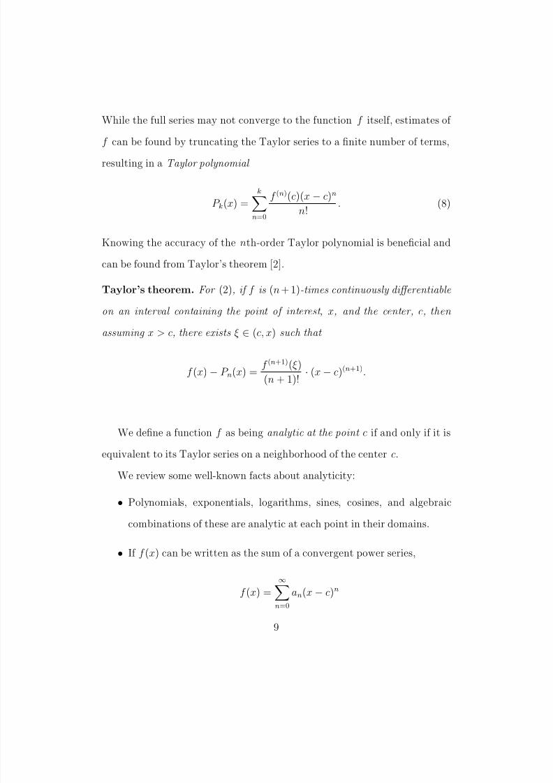
While the full series may not converge to the function f itself, estimates of

f can be found by truncating the Taylor series to a finite number of terms,

resulting in a Taylor polynomial

P k(x) =k

n=0

f (n)(c)(x − c)n

n!. (8)

Knowing the accuracy of the nth-order Taylor polynomial is beneficial and

can be found from Taylor’s theorem [2].

Taylor’s theorem. For (2), if f is (n + 1)-times continuously differentiable

on an interval containing the point of interest, x, and the center, c, then

assuming x > c, there exists ξ ∈ (c, x) such that

f (x) − P n(x) =f (n+1)(ξ)

(n + 1)!· (x − c)(n+1).

We define a function f as being analytic at the point c if and only if it is

equivalent to its Taylor series on a neighborhood of the center c.

We review some well-known facts about analyticity:

• Polynomials, exponentials, logarithms, sines, cosines, and algebraic

combinations of these are analytic at each point in their domains.

• If f (x) can be written as the sum of a convergent power series,

f (x) =∞n=0

an(x − c)n

9



for all x near c, then it is analytic at its center, and an = f (n)(c)

n!; i.e.

the power series must coincide with the Taylor series.

A few well-known Taylor series centered at zero are listed below.

ex =∞n=0

xn

n!= 1 + x +

x2

2!+

x3

3!+

x4

4!+

x5

5!+ . . . x ∈ R. (9)

1

1 − x=

∞n=0

xn = 1 + x + x2 + x3 + x4 + x5 + . . . x ∈ (−1, 1). (10)

Keeping these ideas in mind, let us revisit the simple IVP (2),

y = y

y(0) = b. (11)

Let us for the moment assume that this IVP has an analytic solution y(x).

Can we determine its Taylor series expansion from only (11)? Evaluating the

differential equation at x = 0 yields

y(0) = y(0).

Differentiating both sides of (11) with respect to x, we find that

y(x) = y(x).

10



Substituting in the identity (11), the expression reduces to

y(x) = y(x). (12)

Evaluating this expression at x = 0,

y(0) = y(0).

Let us differentiate both sides of (12) with respect to x again. We obtain

y(x) = y(x),

and after substituting, the identity (11), we obtain

y(x) = y(x).

Evaluating this expression at x = 0 yields

y(0) = y(0).

By induction, the nth-derivative can be shown to be

y(n)(x) = y(x),

11



whence we have

y(n)(0) = y(0). (13)

Since we are assuming y is analytic at x = 0, y must take the form

y(x) = y(0) +∞n=1

y(n)(0)(x − 0)n

n!

for all x in a neighborhood of 0. Substituting (13) into this equation gives

y(x) = y(0) +∞n=1

y(0)xn

n!,

which can be rewritten by (9) as

y(x) = y(0)∞n=0

xn

n!= y(0)ex.

After invoking the initial condition,

y(x) = bex,

which is equivalent to what we found previously.

4 Taylor Series Algorithm

The method that we used to solve the IVP (11) can easily be generalized to

any IVP of the form (2). The algorithm for finding the solution to (2) can

12



be condensed into the following steps [3]: given y = F (x, y),

1. Evaluate the IVP at x = c to obtain the value of y(c).

2. Determine whether F (x, y) is differentiable.

3. If so, differentiate both sides of the differential equation and substitute

y = F (x, y) to obtain a new equation y = F 2(x, y).

4. Evaluate this new equation at x = c to obtain the value of y(c).

5. Repeat this two-step process until a satisfiable number n of derivatives

y(k)(c) has been determined.

6. Substitute the known values into the formula for the Taylor series,

creating the Taylor polynomial of degree n, P n(x).

As another illustration of the technique, consider the IVP

y = xy

y(0) = b. (14)

Substituting x = 0 yields

y(0) = 0.

Differentiating both sides of (14) with respect to x, we obtain

y(x) = y(x) + xy(x),

13



and after substituting,

y(x) = y(x) + x2y(x).

Evaluating this expression at x = 0,

y(0) = y(0).

Repeating this method will provide the following iterations:

y(x) = 3xy(x) + x3y(x) ⇒ y(0) = 0

y(4)(x) = 3y(x) + 6x2y(x) + x4y(x) ⇒ y(4)(0) = 3y(0)

y(5)(x) = 15xy(x) + 10x3y(x) + x5y(x) ⇒ y(5)(0) = 0

y(6)(x) = 15y(x) + 45x2y(x) + 15x4y(x) + x6y(x) ⇒ y(6)(0) = 15y(0)

...

Assuming that the solution y is analytic, we can express it near x = 0 as

the Taylor series

y(x) = y(0) +∞n=1

y(n)(0)(x − 0)n

n!.

14



Substituting the nth-derivative into this equation provides

y(x) = y(0) +

y(0)x2

2!+

3y(0)x4

4!+

15y(0)x6

6!+ · · ·

= y(0)

1 +

1

2

x21

+1

8

x22

+1

48

x23

+ · · ·

= y(0)

1 +

1

1!

x2

2

1

+1

2!

x2

2

2

+1

3!

x2

2

3

+ · · ·

.

Making a logical guess at the series, this expression suggests that

y(x) = y(0)∞n=0

1

n!

x2

2

n

= y(0) exp

x2

2

.

We could prove this formula by an induction; however, it is just as easy to

check that the function. Note that it solves the differential equation y(x) =

xy(x).

d

dx

y(0) exp

x2

2

= y(0)x exp

x2

2

= xy(0) exp

x2

2

for all x. Hence, this expression is a solution. After invoking the initial

condition, this solution becomes

y(x) = b exp

x2

2

.

We encourage the reader to double check this result using familiar techniques

such as separation of variables.

15



How would we apply this algorithm to the general case of y = F (x, y)?

In both cases one must note that the function F (x, y) had to be repeatedly

differentiable for this technique to work. Thus, let us assume F is analytic

at (c, b).

If one defines F 1(x, y) = F (x, y), then by the chain rule

y(x) =∂F 1(x, y(x))

∂x+

∂F 1(x, y(x))

∂yy(x)

=∂F 1(x, y(x))

∂x +∂F 1(x, y(x))

∂y F 1(x, y(x))

=: F 2(x, y(x)),

and

y(x) =∂F 2(x, y(x))

∂x+

∂F 2(x, y(x))

∂yy(x)

=

∂F 2(x, y(x))

∂x +

∂F 2(x, y(x))

∂y F 1(x, y(x))

=: F 3(x, y(x)).

This recursion raises serval important questions:

• Will this pattern hold indefinitely?

• Is the assumption that an analytic solution exists even valid?

• If so, what is the utility of this recursion?

We discuss these questions in the next section.

16



5 The Main Result

Theorem 1. Consider the initial value problem

y = F (x, y)

y(c) = b,(15)

and assume that F is analytic at (c, b). Then the unique solution of this IVP

is given by the analytic function

y(x) = b +∞n=1

F n(c, b)(x − c)n

n!,

where F n(x, y) is defined recursively by

F 1 = F

F n+1 =∂F n

∂x+

∂F n

∂yF 1

.

To the author’s knowledge, this explicit form of the Taylor Series solution

is the only technique for finding explicit solutions to any first-order, analytic

ordinary differential equation of the form (15).

Formally expressing two theorems will aid in the proof. The first is a pre-

cise statement of the existence and uniqueness theorem mentioned in Section2 [1].

Picard-Lindelof theorem. Consider initial value problem (15). If F is

17



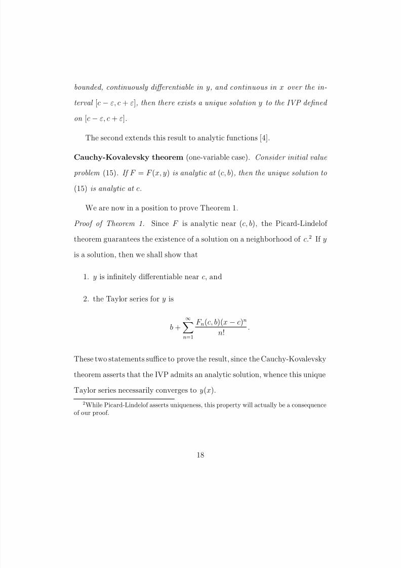
bounded, continuously differentiable in y, and continuous in x over the in-

terval [c − ε, c + ε], then there exists a unique solution y to the IVP defined

on [c − ε, c + ε].

The second extends this result to analytic functions [4].

Cauchy-Kovalevsky theorem (one-variable case). Consider initial value

problem (15). If F = F (x, y) is analytic at (c, b), then the unique solution to

(15) is analytic at c.

We are now in a position to prove Theorem 1.

Proof of Theorem 1. Since F is analytic near (c, b), the Picard-Lindelof

theorem guarantees the existence of a solution on a neighborhood of c.2 If y

is a solution, then we shall show that

1. y is infinitely differentiable near c, and

2. the Taylor series for y is

b +∞n=1

F n(c, b)(x − c)n

n!.

These two statements suffice to prove the result, since the Cauchy-Kovalevsky

theorem asserts that the IVP admits an analytic solution, whence this unique

Taylor series necessarily converges to y(x).

2While Picard-Lindelof asserts uniqueness, this property will actually be a consequenceof our proof.

18



Being a solution to the differential equation, we have

y(x) = F 1(x, y(x)), (16)

for all x in some neighborhood N of c. Thus,

y(c) = F 1(c, b)

after applying the initial conditions. Observe that y is differentiable on N ,

since F 1 is (infinitely) differentiable and y is differentiable. Differentiating

both sides of (16) using the chain rule gives

y(x) =∂

∂x(F 1(x, y(x)))

=∂F 1

∂x(x, y(x)) +

∂F 1

∂y(x, y(x)) · y(x)

= ∂F 1∂x (x, y(x)) + ∂F 1∂y (x, y(x)) · F 1(x, y(x)),

after substituting (16). Thus,

y(x) = F 2(x, y(x)). (17)

In particular, two facts are gained:

1. y(c) = F 2(c, b), and

2. y itself is differentiable, since both F 2 and y are differentiable.

19



Differentiating both sides of (17) gives

y(x) =∂F 2

∂x(x, y(x)) +

∂F 2

∂y(x, y(x)) · y(x),

which reduces to

y(x) =∂F 2

∂x(x, y(x)) +

∂F 2

∂y(x, y(x)) · F 1(x, y(x)),

after substituting (16). Then,

y(x) = F 3(x, y(x)). (18)

Again, two new facts are gained:

1. y(c) = F 3(c, b), and

2. y itself is differentiable, since both F 3 and y are differentiable.

Now, assume by induction that for some n ≥ 3 we have

y(n)(x) = F n(x, y(x)) (19)

for x ∈ N . Observe y(n) is itself differentiable, being a composition of differ-

ential functions. Then,

y(n+1)(x) =d

dx

y(n)(x)

=

∂F n

∂x(x, y(x)) +

∂F n

∂y(x, y(x)) · y(x),

20



which reduces to

y(n+1) = ∂F n∂x

+ ∂F n∂y

· F 1,

after substituting (16). Thus,

y(n+1)(x) = F n+1(x, y(x))

for all n ≥ 0. In particular, this induction proves that

y(n)(c) = F n(c, b)

for any n ≥ 1. Thus, the Taylor series for y takes the form

∞n=0

y(n)(c, b)(x − c)n

n!= b +

∞n=1

F n(c, b)(x − c)n

n!.

Worth noting is the fact that we have proven more than our initial state-

ment.

Corollary 1. If F is infinitely differentiable near (c, b), then the IVP (2)

has a unique solution y such that

1. y is infinitely differentiable, and

21



2. the Taylor series for y is

b +∞n=1

F n(c, b)(x − c)n

n!;

however, no guarantee exists that the Taylor series converges to y.

As an example, consider

F (x, y) =

−2exp(−x−2)

x3 x = 0

0 x = 0,

then the unique solution is

y(x) =

exp(−x−2) x = 0

0 x = 0.

Corollary 2. If F is k-times continuously differentiable near (c, b), then

1. y is k-times continuously differentiable, and

2. the kth order Taylor polynomial for y is

P k(x) = b +k

n=1

F n(c, b)(x − c)n

n!.

Moreover, if F is (k + 1)-times differentiable near (c, b), then for any x

22



near c there exists (ξ, ζ ) near (c, b) such that

y(x) − P k(x) =F k+1(ξ, ζ )(x − c)k+1

(k + 1)!.

The Taylor polynomial result was also proven during the proof of the

theorem. The error statement is a direct application of Taylor’s Theorem,

using the fact thaty(k+1)

(x

) =F k+1(

x, y(

x)) for all

xnear

c.

6 Results

Again, let us return to (3) and attempt to use Theorem 1 to solve the problem.

Note that F (x, y) = y is a polynomial, so it is analytic at any point. Hence,

Theorem 1 can be applied. Setting

F 1 = y,

we find

F 2 =∂F 1

∂x+

∂F 1

∂yF 1 = 0 + 1 · y.

Similarly,

F n+1 =

∂F n

∂x +

∂F n

∂y F 1 = 0 + 1 · y.

Thus,

F n(0, 1) = 1

23



for all n ≥ 1. Substituting,

y(x) = 1 +∞n=1

(1)(x − 0)n

n!=

∞n=0

(x)n

n!= ex,

coinciding with what was found solving the IVP using separation and inte-

gration and using the Taylor Series Solution algorithm.

Now, let us return to (4) and attempt to use Theorem 1 to solve this

problem. Note that if F (x, y) = y2 is a polynomial, so it is analytic at any

point. Thus, Theorem 1 can be applied. Setting

F 1 = y2,

we find

F 2 =∂F 1

∂x

+∂F 1

∂y

F 1 = 0 + 2y · y2 = 2y3

F 3 =∂F 2

∂x+

∂F 2

∂yF 1 = 0 + 6y2 · y2 = 6y4

F 4 =∂F 3

∂x+

∂F 3

∂yF 1 = 0 + 24y3 · y2 = 24y5.

Similarly,

F n = n!yn+1.

Thus,

F n(0, b) = n!bn+1

24



for all n ≥ 1. Substituting,

y(x) = b +∞n=1

(n!bn+1)(x − 0)n

n!

= b + b

∞n=1

(bx)n

= b

∞n=0

(bx)n

=b

1 − bx

,

using (10). This expression coincides with what was found solving the IVP

using separation and integration.

Now, let us return to (6). First, sin(xy) is analytic, as it is the composition

of sine with a product of polynomials. Theorem 1 can be applied. Let

F 1 = sin(xy),

whence F 1(1, 2) = sin(2). The next iteration reduces to

F 2 = y cos(xy) + x cos(xy)sin(xy),

whence F 2(1, 2) = cos(2) (2 + sin(2)). Continuing this iterative process can

be computationally intensive; however, after finding the next two recursions,substituting the initial conditions, and substituting into the Taylor series,

25



the third-order Taylor polynomial is

P 3(x) =2 + sin(2)(x − 1) + cos(2) (2 + sin(2))(x − 1)2

2

+−5 sin(2) + 2 cos(2) sin(2) + 2 sin(2) cos(2)2 − 4 + 6 cos(2)2

(x − 1)3

6.

A decimal approximation of the ninth-order Taylor polynomial to four sig-

nificant figures is

P 9(x) =1.091 + 0.9093x − 0.6053(x − 1)2 − 1.325(x − 1)3

+ 0.4268(x − 1)4 + 1.738(x − 1)5 − 0.1539(x − 1)6

− 2.613(x − 1)7 − 0.3907(x − 1)8 + 4.075(x − 1)9.

The truncated Taylor series does a very good job approximating the solution

after as few as three to five iterations. Plotting these expressions versus the

numerical approximations of the solution using both the Euler technique and

the Runga-Kutta technique shows this relationship (see Figure 2).

26



Figure 2. Comparison for y = sin(xy).

This plot illustrates a potential downside of analytic solutions: the radius of

convergence might unexpectedly be smaller than one would like.

7 Linear Differential Equations

The general form of a first-order linear nonhomogeneous ordinary differential

equation is

y

(x) = q(x)y(x) + p(x)

y(c) = b, (20)

27



with corresponding homogeneous ODE

y(x) = q(x)y(x). (21)

From the previous discussion the general solution to (20) is the superposition

of the general solution to (21) and a particular solution to (20). For sake of

consistency, call these solutions yq and y p, respectively, so that the solution

to (20) is

y(x) = kyq(x) + y p(x).

Theorem 2. If p, q are both analytic at c, then the unique solution to (20)

is

y(x) = b + b

∞n=1

qn(c)(x − c)n

n!+

∞n=1

pn(c)(x − c)n

n!,

where qn(x) is defined by

q1 = q

qn+1 = qn + qnq1

and pn(x) is define by

p1 = p

pn+1 = pn + qn p1

.

28



A consequence of this result is that it gives explicit formulas for both yq and

y p, namely

yq(x) = b + b

∞n=1

qn(c)(x − c)n

n!,

and

y p(x) =∞n=1

pn(c)(x − c)n

n!.

Proof of Theorem 2. Theorem 1 asserts that this IVP has an analytic solution.

Since

y(x) = q(x)y(x) + p(x),

this equation implies

F 1(x, y) = q1(x)y + p1(x). (22)

Since q and p are analytic,

F 2(x, y) =∂F 1(x, y)

∂x+

∂F 1(x, y)

∂yF 1(x, y)

=∂ (q1(x)y + p1(x))

∂x+

∂ (q1(x)y + p1(x))

∂y(q1(x)y + p1(x))

= q1(x)y + p1(x) + q1(x) (q1(x)y + p1(x))

= (q1(x) + q1(x)q1(x)) y + ( p1(x) + q1(x) p1(x))

= q2(x)y + p2(x)

after substituting (22) and rearranging.

29



Now, assume

F n = qny + pn

for some n ≥ 2; then,

F n+1 =∂F n

∂x+

∂F n

∂yF 1

=∂ (qny + pn)

∂x+

∂ (qny + pn)

∂y(q1y + p1)

=qn

y+

pn +

qn(

q1

y+

p1)

= (qn + qnq1)y + ( pn + qn p1)

= qn+1y + pn+1.

Thus,

F n(x, y) = qn(x)y + pn(x)

for all n.

Substituting into the explicit formula given by (7) gives

y(x) = b +∞n=1

F n(c)(x − c)n

n!

= b +∞n=1

(qn(c)d + pn(c))(x − c)n

n!

= b + b

∞

n=1

qn(c)(x − c)n

n!

+∞

n=1

pn(c)(x − c)n

n!

.

A quick observation of this result, in comparison to the result for (21) using

30



Theorem 1, confirms that

yq(x) = b + b

∞n=1

qn(c)(x − c)n

n!,

and

y p(x) =∞n=1

pn(c)(x − c)n

n!.

Now, (5) can be reevaluated using the previous recursion statements.

First, we must identify the various parts of the differential equation:

q1 = 1; p1 = exp(2x).

With these initial expressions, the recursive statement can be employed such

that

q2 = q1 + q1 · q1 = (1) + (1) · (1) = 1,

q3 = q2 + q2 · q1 = (1) + (1) · (1) = 1,

and, by induction,

qn+1 = qn + qn · q1 = (1) + (1) · (1) = 1.

31



Also,

p2 = p1 + q1 · p1 = (exp(2x)) + (1) · (exp(2x)) = 3 exp(2x),

p3 = p2 + q2 · p1 = (3 exp(2x)) + (1) · (exp(2x)) = 7 exp(2x),

p4 = p3 + q3 · p1 = (7 exp(2x)) + (1) · (exp(2x)) = 15 exp(2x),

and, by induction,

pn+1 = pn + qn · p1 = (2n − 1) exp(2x).

Thus,

y(x) = (0) + (0)∞n=1

(1)(x − 0)n

n!+

∞n=1

(2n − 1)(x − 0)n

n!

=∞

n=1

2nxn

n!

−∞

n=1

xn

n!

=

∞n=0

(2x)n

n!−

(2x)0

0!

−

∞n=0

xn

n!−

x0

0!

= e2x − 1 − ex + 1

= e2x − ex.

This expression is exactly what was previously found by using the method

of undetermined coefficients. The novelty of Theorem 2 is that it produces a

particular solution without requiring the solution to the related homogeneous

ODE to be known beforehand. As an example, let us attempt to find the

32



particular solution to

y = y + ex

y(0) = 0. (23)

Now, (23) can be reevaluated using the previous recursion statements.

First, we must identify the various parts of the differential equation:

q1 = 1; p1 = exp(x).

With these initial expressions, the recursive statement can be employed such

that

q2 = q1 + q1 · q1 = (1) + (1) · (1) = 1,

q3 = q2 + q2 · q1 = (1) + (1) · (1) = 1,

and, by induction,

qn = qn−1 + qn−1 · q1 = (1) + (1) · (1) = 1.

Also,

p2 = p1 + q1 · p1 = (exp(x)) + (1) · (exp(x)) = 2 exp(x)

p3 = p2 + q2 · p1 = (2 exp(x)) + (1) · (exp(x)) = 3 exp(x)

p4 = p3 + q3 · p1 = (3 exp(x)) + (1) · (exp(x)) = 4 exp(x)

33



and, by induction,

pn = pn−1 + qn−1 · p1 = n exp(x).

Then, the particular solution to (23) is

y p(x) =∞n=1

(n exp(0)(x − 0)n

n!

=

∞n=0

nxn

n!

= xex.

8 Conclusions

The exploitation of differential equations has allowed a substantial increase

in the understanding of nature, but limitations to accurately and efficiently

solving differential equations still persist. Any grasp of the analytic solutions

for sets of differential equations will only aid the effort.

The theorems presented provide a convenient way to gauge the sensitivity

of a solution to its initial conditions (c, b), and to parameters such as a in

the classic rocket problem modeled by y(x) = ya, a ≤ 2 with the initial

conditions bounded away from (0, y). Also, noting that a formal solution

exists regardless of the radius of convergence for the solution is beneficial; it

can identif candidate solutions and still provide numerical approximations.

34



The most convenient characteristic of this technique is that it solves ODEs

using only differentiation techniques and hence is accessible to any calculus

student. Although this paper only examined a power series approach to

analytically solving first-order ODEs in standard form, many new directions

are fostered from this discussion.

References

[1] P. Blanchard, R.L. Devaney, G.R. Hall. Differential Equations. Second

Edition. Pacific Grove, CA: Brooks/Cole, 2002.

[2] W. Kosmala. A Friendly Introduction to Analysis. Second Edition. Upper

Saddle River, New Jersey: Pearson Prentice Hall, 2004.

[3] R.K. Nagel, E.B. Saff, A.D. Snider. Fundamentals of Differential Equa-

tions. Sixth Edition. Boston: Pearson-Addison Wesley, 2004.

[4] E.C. Zachmanglou and D.W. Thoe. Introduction to Partial Differential

Equations. New York: Dover Publications, Inc., 1986.

35

Documents

ODE Solving