Embed Size (px)
Citation preview

Lecture 6: Labour income taxation (1)
Antoine Bozio
Paris School of Economics (PSE)
Ecole des hautes etudes en sciences sociales (EHESS)
Master APE and PPDParis – October 2021
1 / 149

Labour income taxation
1 Do tax cut pay for themselves ?• Are we above the Laffer curve ?
2 How to redistribute to the poor ?• Do benefits lead to poverty traps ?• Does workfare works ?
3 Should we introduce basic income/flat tax ?• Is it utopia, nightmare or the future of tax design ?
4 How much can we tax the rich ?• Do high taxes on top incomes soak the rich or make
everyone worse off ?
2 / 149

Outline of the lecture 6
I. Incidence : who pays taxes ?
1 Theory2 Empirical estimates
II. Labour supply responses
1 Structural labour supply estimates2 Quasi-experimental labour supply estimates3 Macro vs micro estimates
III. Policy : Transfer to the poor
1 Traditional welfare2 Optimal transfer system3 Workfare or EITC-like policies
3 / 149

Outline of the lecture 7
IV. Elasticity of taxable income
1 Conceptual framework2 Early ETI studies3 Recent ETI studies
V. Optimal labour taxation
1 Conceptual framework2 Mirrlees model3 Generalized optimal labour taxation models
VI. Policy : Taxing top incomes
1 What top marginal tax rate ?2 Issue of international mobility3 Policy debate : supply side vs optimization vs rent seeking
4 / 149

History of income taxation
• First attempts at general income taxation (18th c.)• First discussion about measurement of national income• Attempts at general income taxation (Touzery, 1994)
e.g., taille tarifee in France in 1715
• Schedular income tax (19th c.)• Different tax schedule by type of income
e.g., land, farming, trades, pensions, etc.• Income tax, a British invention :
• 1799 income tax by PM William Pitt the Younger• 1803 income tax by PM Henry Addington• 1842 income tax with PM Robert Peel
• France income tax on capital income (impot sur le revenudes valeurs mobilieres) in 1872
5 / 149

History of income taxation
• First modern income tax• 1891 in Prussia• 1909 in the U.K.• 1913 in the U.S. (Mehrotra, 2013)• 1914 in France (Piketty, 2001 ; Delalande, 2011)
• Comprehensive and progressive• Comprehensive : all income sources taxed in the same tax
schedule• Progressive : only on top incomes• But small : top marginal tax rates at 3%
• Large increases with war efforts• WWI : top rates reached 40% to 70%• WWII : top rates reached 70% to 97%
6 / 149

Figure 1 – Top marginal tax rates (1900–2013)
0%
10%
20%
30%
40%
50%
60%
70%
80%
90%
100%
1900 1910 1920 1930 1940 1950 1960 1970 1980 1990 2000 2010
Mar
gina
l tax
rat
e ap
plyi
ng to
the
high
est i
ncom
esU.S.
U.K.
Germany
France
Source : Piketty (2013), Fig. 14.1
7 / 149
Types of labour income taxation
1 Income tax• Taxation of labour and capital income• Progressive tax : increasing average tax rate
2 Social Security contributions (SSCs)• Confer entitlement to receive a future social benefit• Taxation of earnings (not capital income)• Nominally split between employee and employers• Usually capped at threshold
3 Means-tested benefits• Assessed at household level• Child benefits, housing benefits, minimum income, etc.• Analysis similar to labour taxation
8 / 149

Figure 2 – Income tax as a % of GDP, 1990–2017
0
5
10
15
20
25
30
35
40
1990 1995 2000 2005 2010 2015
Sh
are
of
GD
P (
in p
erc
en
tag
e)
Canada Denmark France Germany Italy
Mexico Sweden U.K. U.S.
Source : OECD.Stat
9 / 149

Figure 3 – Income tax as a % of GDP, 1990–2017
0,0
1,0
2,0
3,0
4,0
5,0
6,0
7,0
8,0
9,0
10,0
1990 1995 2000 2005 2010 2015
Sh
are
of
GD
P (
in p
erc
en
tag
e)
Argentina Brazil Cameroon Egypt Indonesia
Source : OECD.Stat
10 / 149

Figure 4 – Income tax as a share of GDP (1914–2014)
0%
2%
4%
6%
8%
10%
12%
14%
16%
1914 1924 1934 1944 1954 1964 1974 1984 1994 2004 2014
Pe
rce
nta
ge
of
GD
PUnited Kingdom
United States
France (IR, CSG and CRDS)
France (IR)
Source : Andre and Guillot, IPP Briefing Note, No. 12, 2014.
11 / 149

Figure 5 – Social Security Contributions as a % of GDP, 1965–2014
0
2
4
6
8
10
12
14
16
18
20
1965 1970 1975 1980 1985 1990 1995 2000 2005 2010
FRANCE
US
UK
OECD
GERMANY
JAPAN
Source : OECD.Stat
12 / 149

Figure 6 – Employer SSCs as a % of GDP, 1965–2014
14
12 FRANCE
10
8
6 GERMANY
JAPAN
4
OECDJAPAN
4
US
UK
2
0 1965 1970 1975 1980 1985 1990 1995 2000 2005 2010
Source : OECD.Stat
13 / 149

Mean-tested benefits
• Negative average taxation• Benefits similar to tax credit• Negative tax payment
• Marginal tax rates• Means-testing means that additional euro earned is tax
away
e.g., 100% taper rate = 100% MTR
• Common to find high MTR in benefit design
• Budget constraints• Representation of disponible income by hours worked• Slope is 1-MTR
14 / 149

Figure 7 – Budget constraint for French single earner (2014)
0
500
1000
1500
2000
2500
0% 50% 100% 150% 200%
Disp
osab
le in
com
e (m
onth
ly e
uros
)
Labour income pre tax and benefits (as a fraction minimum wage)
Wage (net of tax)
Income support
Income tax
Working tax credit (PA)
Housing benefits
Disposable income
Source : Ben Jelloul, Bozio, Cottet and Fabre, IPP, April 2017.
15 / 149

Figure 8 – Benefits for U.S. single earner and two children (2008)
Source : Maag et al. (2012), Fig. 1.
16 / 149

I. Incidence : Who pays taxes ?
1 Conceptual framework with tax-benefit linkage
2 Empirical evidence for employer SSCs
3 Evidence for income tax and benefits
17 / 149

Conceptual framework with tax-benefit linkage
• Standard general equilibrium model of tax incidence withcompetitive markets (Feldstein, 1974)
• Labour demand• Production function F (.) is assumed to be homogeneous of
degree one with two types of workers T and C .• Labor cost : zk = wk(1 + τk)
wk : posted wageτk : payroll tax rate on employers
• σ : elasticity of substitution between workers
• Labour supply with tax benefit linkage• wk ≡ wk(1 + qτk) the perceived wage of workers of type k• q : extent to which employees value employer contributions• ηS : elasticity of labor supply
18 / 149

Pass-Through Formula
• Pass-through ρ of employer SSCs to the wage oftreated workers relative to control workers
ρ =d ln
(wT
wC
)d ln (1 + τT )
≈ −σ + ηS · qσ + ηS
• Three polar cases :
(1) Full linkage (q = 1) ⇒ full shifting to workers (ρ ≈ 1)(2) No linkage (q = 0) and σ � ηS ⇒ full shifting (ρ ≈ 1)
(3) No linkage (q = 0) and ηS � σ ⇒ no shifting (ρ ≈ 0)
Case (2) is the usual assumptions in the laborsupply/elasticity of taxable income literature
19 / 149

Figure 9 – Incidence with tax-benefit linkage
Wage rate
L0
Supply S(p)
Demand D(p)
wE0
Labour supply
0
20 / 149

Figure 10 – Incidence with tax-benefit linkage
Wage rate
L0
Supply S(p)
D(p+t)
Demand D(p)
W1
L 1
w
SSCs increase
E0
Labour supply
E1
0
21 / 149

Figure 11 – Incidence with tax-benefit linkage
Wage rate
L0
W
Supply S(p)
D(p+t)
Demand D(p)
W1
L 1
w
SSCs increase
E0
E2
Labour supply
E1
0
L2
benefit value
2
22 / 149

Empirical estimates : SSC
• Textbook view• “knowledge of statutory incidence tells us essentially
nothing about who really pays the tax” (Rosen, 2002)• “payroll taxes are borne fully by workers” (Gruber, 2007)
• But relatively little empirical evidence to date
23 / 149

Empirical estimates : SSC
• Macro evidence• Labour income shares fairly stable• Cross-country studies (Brittain, 1971 ; OECD, 1990 ;
Tyrvainen, 1995 ; Alesina and Perotti, 1997 ; Daveri andTabellini, 2000 ; Nunziata, 2005 ; Ooghe et al, 2003)
• Early micro studies• Hamermesh (1979) ; Neubig (1981) ; Holmlund (1983)
• Quasi-experimental studies• Gruber (1994) : Mandated maternity benefits• Anderson and Meyer (1997, 2000) : US UI• Bennmarker et al. (2009) ; Korkeamaki (2011) ; Lehmann
et al. (2013) : reductions in SSCs
24 / 149

Gruber (JOLE, 1997)
• The Chilean reform• Chile privatized its public pension system in 1981• Large cut in SSCs• Expected increase in private pension savings
• Methodology• Time-series and cross-section estimation• Use firm data and firm-level SSC change
• Results• No employment effect and full-shifting of SSCs to wages
(i.e., wage increase of similar magnitude to drop in SSC)
25 / 149
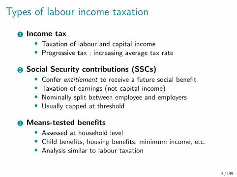
Gruber (JOLE, 1997)• Difference Specification
∆log(Wijt/Eijt) = a + b1∆tijt + eijt
• Triple DiD (across blue and white collar)
Table 1 – Coefficient on Contributions/Wages inCross-Sectional Regressions
Pooled Blue-collar White-Collar
Wages Employment Wages Employment Wages Employment
Basic difference -1.120 0.008 -0.899 0.190 -1.350 -0.183(0.099) (0.106) (0.108) (0.130) (0.172) (0.170)
DDD -1.022 -0.113(0.180) (0.165)
N 6,066 6,066 3,298 3,298 2,768 2,768
Source : Gruber (1997), Tab. 3., p. S95.
26 / 149
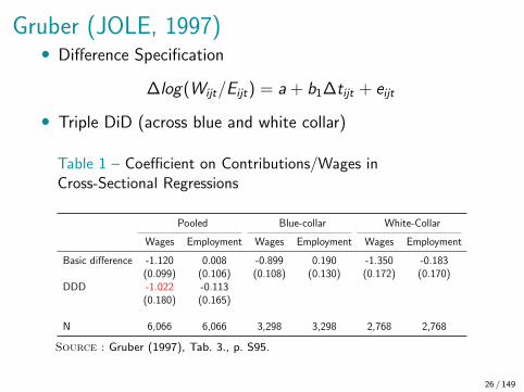
Saez et al. (QJE, 2012) – Greece• The 1992 Greek reform
• Greece has high SSC rates (28% employer, 16% employee)• SSCs up until a threshold (2432 euros monthly earnings)• Increase of threshold to 5,543 euros for new entrants⇒ Reform led to different SSC schedules for adjacent cohort
• Methodology : Regression Discontinuity Design• RDD approach based on date of entry• Estimate long-run incidence effects• Use administrative data from Greek social insurance
• Results• No labour supply effect (neither intensive nor extensive)• Incidence of SSCs similar to nominal incidence (i.e.,
employer SSCs fall on employers, employee SSCs fall onemployees)
27 / 149

Figure 12 – First stage : Average Tax Rates Above Old Cap
Source : Saez et al. (2012), Fig. V.A, p. 522.
28 / 149
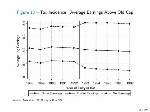
Figure 13 – Tax Incidence : Average Earnings Above Old Cap
Source : Saez et al. (2012), Fig. V.B, p. 522.
29 / 149

Table 2 – Tax Incidence Effects : RDD estimates
Sample : 1988–1997 1991–1994 1988–1997 1988–1997 1988–1997entrants entrants only entrants entrants entrants
(1) (2) (3) (4) (5)
Panel B. Gross, posted, and net earnings (above old cap)
Log gross earnings z 0.031 0.033 0.029 0.021 0.040(0.007) (0.012) (0.007) (0.011) (0.016)
Log posted earnings w -0.013 -0.009 -0.015 -0.021 0.001(0.008) (0.013) (0.008) (0.012) (0.017)
Log net earnings c -0.047 -0.043 -0.050 -0.055 -0.031(0.009) (0.014) (0.009) (0.013) (0.018)
Number of observations 50,084 18,846 50,084 50,084 50,084
ControlsLinear entry date trends Yes Yes Yes Yes YesMonthly dummies Yes Yes YesQuadraticdate trends Yes YesCubic entry date trends Yes
Source : Saez et al. (2012), Tab. V, p. 523.
30 / 149

Saez, Schoefer and Seim (AER, 2019) – Sweden
• The Swedish reform• 2007 cut to payroll tax rate (from 31.4% to 21.3%) for
workers aged 19–25• 2009 cut to 15.5% for workers aged 19–26• Reform repealed in 2015-16
• Methodology (1) : worker-level• RDD approach based on age• Estimate long-run incidence effects + employment• Use administrative data from Swedish social insurance
• Results• No shifting at individual level to wages (100% pass-through
to firms)• Large impact on employment
31 / 149

Figure 14 – The effect of the payroll tax cut on wages
Source : Saez, Schoefer and Seim (2019), Fig. 2, p. 1727.
32 / 149

Figure 15 – Employment impact
Source : Saez et al. (2019).
33 / 149

Saez et al. (AER, 2019) – Sweden
• Methodology (2) : firm-level• DiD between firms with high share of young vs low share• Estimate impact on scale (employment, valued-added,
profit, etc.)• Estimate firm-level incidence (impact on total wage)• Merge employee data with firm-level accounting data
• Results• Large impact on activity (+value-added, +employment, +
profit)• Large impact on wage of all workers• Incidence : fully shifted to workers at firm-level
34 / 149
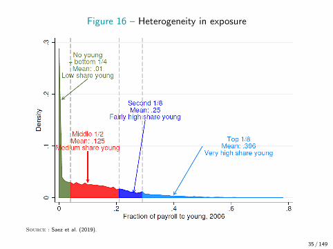
Figure 16 – Heterogeneity in exposure
Source : Saez et al. (2019).
35 / 149

Figure 17 – Net wage on firms with high share of young
Source : Saez et al. (2019).
36 / 149

Figure 18 – Average labour cost per worker : high vs medium shareof young
Source : Saez et al. (2019).
37 / 149

Bozio, Breda and Grenet (2019) – France
• French SSC reforms• Exploit three uncapping reforms in France• Different tax-benefit linkage
• Methodology• DD approach based on pre-reform earnings w.r.t threshold• Estimate long-run incidence effects• Use administrative data (DADS data)
• Results• Incidence of SSCs on employers for reforms with no
tax-benefit linkage• Incidence of SSCs on employees in reform with strong
tax-benefit linkage
38 / 149

Figure 19 – Marginal Employer SSC Rates, Non-Executives,1976–2010
+9.5 ppts
+8.2 ppts
+7.8 ppts
Reform 3Uncappingof heathSSCs
Reform 2Uncappingof familySSCs
Reform 1Increasein pensionsSSCs
0.0
0.1
0.2
0.3
0.4
1976
1977
1978
1979
1980
1981
1982
1983
1984
1985
1986
1987
1988
1989
1990
1991
1992
1993
1994
1995
1996
1997
1998
1999
2000
2001
2002
2003
2004
2005
2006
2007
2008
2009
2010
Year
Under SST1 to 3 SST
Sources : IPP Tax and Benefit Tables (April 2016 ; TAXIPP 0.4)
39 / 149

Figure 20 – Reform 1 : log(z) vs log(w)
-.02
-.01
0.0
1.0
2
-3 -2 -1 0 1 2 3 4 5 6 7 8 9Years since reference year
Hourly labour costGross hourly earnings
Source : Bozio et al. (2018).
40 / 149

Figure 21 – Reform 1 : Pass-Through Rate on Workers – w – withtrends
full pass-through to workers
zero pass-through to workers
-1.0
-0.5
0.0
0.5
1.0
1.5
0 1 2 3 4 5 6 7 8 9Years since reference year
Estimate95% CI
Source : Bozio et al. (2018).41 / 149

Figure 22 – Reform 2 : log(zh) vs log(wh)
-.02
-.01
0.0
1.0
2
-3 -2 -1 0 1 2 3 4 5 6 7 8 9Years since reference year
Labour costGross earnings
Source : Bozio et al. (2018).
42 / 149

Figure 23 – Reform 2 : Pass-Through Rate on Workers– with trends
full pass-through to workers
zero pass-through to workers
-0.5
0.0
0.5
1.0
1.5
2.0
0 1 2 3 4 5 6 7 8 9Years since reference year
Estimate95% CI
Source : Bozio et al. (2018).
43 / 149

Figure 24 – Reform 3 : log(zh) vs log(wh)
-.02
-.01
0.0
1.0
2
-3 -2 -1 0 1 2 3 4 5 6 7 8 9Years since reference year
Labour costGross earnings
Source : Bozio et al. (2019).
44 / 149

Figure 25 – Reform 3 : Pass-Through Rate on Workers – withtrends
full pass-through to workers
zero pass-through to workers
-0.5
0.0
0.5
1.0
1.5
2.0
0 1 2 3 4 5 6 7 8 9Years since reference year
Estimate95% CI
Source : Bozio et al. (2018).45 / 149

Bozio et al. (2018) : SummaryTable 3 – Baseline estimates of pass-through rate on workers
Reform : Reform 1 Reform 2 Reform 3
Dep. var. : log(hourly wage) log(earnings) log(earnings) log(earnings)
Panel A. Without controlling for individual-specific trends
t0+8 0.934*** 0.812*** 0.186 0.384**(0.303) (0.293) (0.166) (0.172)
t0+9 0.906*** 0.969*** 0.215 n/a(0.327) (0.324) (0.170) n/a
Panel B. Controlling for individual-specific trends
t0+8 1.077*** 1.112*** 0.100 0.209(0.318) (0.291) (0.224) (0.133)
t0+9 1.064*** 1.157*** 0.061 n/a(0.335) (0.308) (0.229) n/a
46 / 149

Figure 26 – Meta-Analysis of Payroll Tax Incidence
Gruber & Krueger (1991)
Gruber (1994)
Gruber (1997)
Anderson & Meyer (1997)
Anderson & Meyer (2000)
Komamura & Yamada (2004)
Baicker & Chandra (2006)
Murphy (2007)
Kugler & Kugler (2009)Tax-benefit linkage:
no shifting full shifting
Korkeamäki & Uusitalo (2009)
Bennmarker et al. (2009)
Cruces et al. (2010)
Saez et al. (2012)
Saez et al. (2017)
Bozio et al. (2018)
‐1 ‐0.5 0 0.5 1 1.5 2Estimated pass-through to workers
Tax-benefit linkage:
Strong
Weak
Uncertain
47 / 149

Empirical estimates : income tax
• Limited evidence• General assumption that income tax falls on individuals• In theory, income tax could be incident on employers
e.g., contract of footballers expressed ‘net of tax’
• Evidence• Kubik (JPubE, 2004) : TRA in the U.S. in 1986, drop in
tax rates lead to lower pre-tax wage• Lehman, Marical and Rioux (JPubE, 2013) : in France
incidence of SSCs reduction vs income tax• Bingley and Lanot (JPubE, 2002) : Denmark, partial
shifting of income tax
48 / 149

Empirical estimates : benefits
• Limited evidence• General assumption that benefits benefit individuals• In theory, benefits could be incident on employers
e.g., those on benefits could be paid less
• Evidence• Rothstein (AEJ-policy, 2010) : EITC in the U.S.• Fack (Labour Econ., 2006) : housing benefits in France• Azmat (Quant. Econ., 2019) : WFTC in the U.K.• Garriga and Tortarolo (2020) : tax credit in Argentina
49 / 149

II. Labour supply responses
• Why labour supply matters• If people work less, as response to tax, then limits to
taxation and redistribution• Tax increases will impact the tax base, and raise less
revenues than expected
• Labour supply elasticity• Measures how much labour is reduced when net wage is
reduced
ε =∂logL
∂logw
• Severe challenges to measure ε
50 / 149

II. Labour supply responses
1 Baseline labour supply model
2 Early empirical studies
3 Randomised controlled trials
4 Quasi-experimental evidence
5 Micro vs macro estimates
51 / 149
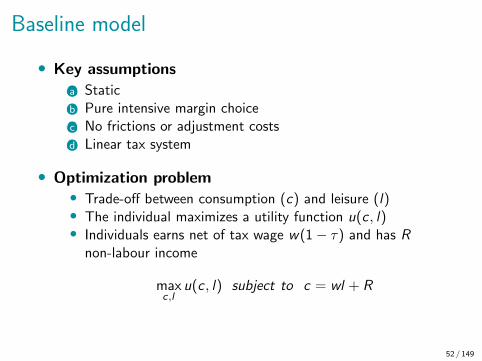
Baseline model
• Key assumptions
(a) Static(b) Pure intensive margin choice(c) No frictions or adjustment costs(d) Linear tax system
• Optimization problem• Trade-off between consumption (c) and leisure (l)• The individual maximizes a utility function u(c , l)• Individuals earns net of tax wage w(1− τ) and has R
non-labour income
maxc,l
u(c , l) subject to c = wl + R
52 / 149

Baseline model• Uncompensated or Marshallian elasticity of labour
supply• FOC : wuc + ul = 0 defines Marshallian labour supply
function lu(w , l)• Uncompensated elasticity of labour supply : εu
εu =w
l
∂lu
∂w
• % change in hours when net wage increase by 1%
• Income effects• Income effect parameter η
η = w∂l
∂R
• Increase in non-labour income leads to decrease in laboursupply
53 / 149

Baseline model
• Compensated or Hicksian elasticity of labour supply• Minimization of cost wl − c subject to the constraint of
u(c , l) >= u leads to Hicksian labour supply function• Compensated elasticity of labour supply : εc
εc =w
l
∂lc
∂w
• Deadweightloss depends on εc
• Slutsky equation
∂l
∂w=∂l c
∂w+ l
∂l
∂R
εu = εc + η
54 / 149

Baseline model
An increase in income tax has three effects :
1 Income effect : lower unearned income⇒ Increases labour supply
2 Income effect : lower after-tax wage⇒ Increases labour supply
3 Substitution effect : lower after-tax wage⇒ Decreases labour supply
⇒ The net effect is theoretically ambiguous ; it is an empiricalquestion.
55 / 149

Surveys
• Labour economics literature• Pencavel (1986) HLE, vol. 1• Heckman and Killingsworth (1986) HLE, vol. 1• Blundell and MaCurdy (1999) HLE, vol. 3
• Public economics literature• Hausman (1985) HPE, vol. 1• Moffitt (2003) HPE, vol. 4
• Econometrics literature• Blundell, MaCurdy and Meghir (1985) HPE, vol. 1
56 / 149

Labour supply elasticities
• Intensive margin• Primary earners (used to be usually men) have low
elasticities (around 0.1).• Secondary earners of the household (typically married
women) have much higher elasticities (between 0.5 and 1).
• Extensive margin• Highly educated men have very low participation elasticities• Low educated men have modest participation elasticities• Married women have much higher elasticities• Lone mothers have very high participation elasticities
57 / 149

Labour supply elasticities
• Blau and Kahn (JOLE, 2007)• Use grouping instrument on data from 1980-2000• Define cells (year/age/education)• Identification from group-level variations
• Results• Married female labour supply elasticity has been falling
sharply• total hours elasticity : 0.4 in 1980 to 0.2 in 2000• effect of husband earnings reduced over time
• The distinction between primary and secondary earnerstends to blur with the increase in female participation
58 / 149

Randomized controlled trial
• Negative income tax (NIT)• Complex set of cash and in-kind benefits in the U.S. in the
1960s• NIT : guaranteed income payment to all poor households,
gradually reduced with earnings• Fear that NIT will reduce labour supply
• Income Maintenance Experiments• First major social experiments in the U.S.• Four large randomized controlled trials (RCT) :
1) New Jersey and Pennsylvania (1968-1972)2) Iowa and North Carolina (1969-1973)3) Gary, Indiana (1971-1974)4) Denver and Seattle (1971-1982)
• Large cost of the experiment (1 billion USD)
59 / 149

Randomized controlled trial• NIT experimented
• Benefit B defined as a function of lump-sum grant G withphaseout rate τ for households with income Y :B = G − τY if Y < G
τ
B = 0 if Y > Gτ
• Gτ is the break-even point
• τ is the marginal tax rate
• Experimental design• Several groups with randomization within each• Around 75 households per group
• Analysis• Rees (JHR 1974)• Munnell (1986) : conference volume on NIT experiments• Ashenfelter and Plant (JOLE, 1990)
60 / 149

Randomized controlled trial
Figure 27 – Parameters of the 11 NIT experiments
Source : Ashenfelter and Plant (1990), Tab. 1.
61 / 149

Randomized controlled trial
• Ashenfelter and Plant (JOLE, 1990)• Analysis of the Denver and Seattle NIT• Present non-parametrics evidence of labour supply effects• Compare actual benefits payments to treated households to
counterfactual benefit payments to control households• Difference in benefits reflects aggregate hours response
• Results• Significant labour supply response but small• Implied earnings elasticities :
• male : 0.1• female : 0.5
• Response of women concentrated along the extensivemargin
62 / 149

Figure 28 – Payments treated vs control
Note : Standard errors are in brackets ; ∗ denotes mean is more than twice its standard error.Source : Ashenfelter and Plant (1990), Tab. 3. 63 / 149

Randomized controlled trial
• Shortcomings of the NIT experiments• Self-reported earnings (with incentives to under-report
earnings)• Selective attrition (no incentives to report when above
breakeven point)• GE effects
• Shortcomings of the analysis• No distinction between extensive/intensive margin• No separate estimation of income effects vs substitution
effects• Hard to identify the key elasticity relevant for policy
purposes
64 / 149

Experience of tax holiday
• Tax holiday in Iceland• In 1986, Iceland announced major reform to income tax
1 Move to tax withholding in 1988 (pay-as-you-earn)2 Change of tax schedule with lower marg. tax rate and
higher tax-free allowance
• To avoid double taxation during transition, no tax chargedover 1987 incomes
• Bianchi, Gudmundsson and Zoega (AER, 2001)• Exploit the 1987 no tax experiment : large and salient tax
variation (4(1−MTR) ' 49%• Data : individual tax returns matched with data on weeks
worked from insurance database• Estimate intertemporal substitution elasticity (work hard in
1987, relax after)
65 / 149

Figure 29 – Employment rate in Iceland (1960-1996)
Sources : Bianchi, Gudmundsson and Zoega (2001), Fig. 1.66 / 149

Macro estimates
• Macroeconomic approach• Macroeconomists exploit long-term trends or cross-country
comparisons• Use aggregate data on hours/tax
• Identification• Calibration technique : find elasticity that best fits the
data/model• Identification is problematic• Similar to regression without controls• But perhaps more relevant to long-run policy questions of
interest
67 / 149

Macro estimates
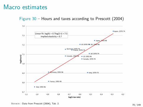
• Edward Prescott• Edward Prescott, American macroeconomist, Nobel prize
2004• “virtually all of the large differences between U.S. labor
supply and those of Germany and France are due todifferences in tax systems”
• Prescott (2004)• Data on hours worked and tax rates for 7 OECD countries• Calibration of GE model
u(c , l) = c − l1+ 1ε
1 + 1ε
• Find that labour supply elasticity ε = 0.7 best matchestimes series
68 / 149
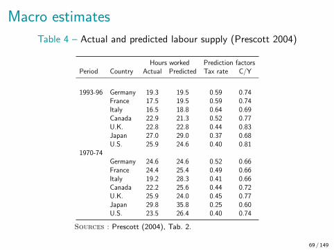
Macro estimates
Table 4 – Actual and predicted labour supply (Prescott 2004)
Hours worked Prediction factorsPeriod Country Actual Predicted Tax rate C/Y
1993-96 Germany 19.3 19.5 0.59 0.74France 17.5 19.5 0.59 0.74Italy 16.5 18.8 0.64 0.69Canada 22.9 21.3 0.52 0.77U.K. 22.8 22.8 0.44 0.83Japan 27.0 29.0 0.37 0.68U.S. 25.9 24.6 0.40 0.81
1970-74Germany 24.6 24.6 0.52 0.66France 24.4 25.4 0.49 0.66Italy 19.2 28.3 0.41 0.66Canada 22.2 25.6 0.44 0.72U.K. 25.9 24.0 0.45 0.77Japan 29.8 35.8 0.25 0.60U.S. 23.5 26.4 0.40 0.74
Sources : Prescott (2004), Tab. 2.
69 / 149
Macro estimates
Figure 30 – Hours and taxes according to Prescott (2004)
Germany 1970-74France, 1970-74
Italy, 1970-73
Canada, 1970-74
US 1970-74
Japan, 1970-74
UK 1970-74
Germany, 1993-96
France, 1993-96
Italy 1993-96
Canada, 1993-96 US 1993-96
Japan, 1993-96
UK, 1993-96
Linear fit: log(h) = 0.7log(1-t) + 7.5
Implied elasticity = 0.7
6,7
6,8
6,9
7,0
7,1
7,2
7,3
7,4
-1,1 -1,0 -0,9 -0,8 -0,7 -0,6 -0,5 -0,4 -0,3 -0,2
log
(ho
urs
)
log(1-tax rate)
Source : Data from Prescott (2004), Tab. 2.70 / 149

Macro estimates
• Macro vs micro estimates• Macro calibrated models need high labour supply
elasticities• Cross-country evidence suggests high correlation between
hours worked and taxes• Micro (within country) evidence suggests small elasticities
• Debate within economists• “Prescott’s provocative paper” (Alesina, Glaeser and
Sacerdote, 2005)• Results confirmed with other calibrations and more data
(Ohanian, Raffo and Rogerson, JME, 2008)• Prescott Nobel Lecture (JPE, 2006)
71 / 149

Macro vs micro : explanations1 Omitted variable
• Labour market regulations (Alesina, Glaeser and Sacerdote,2005)
• Cultural differences between high tax/low tax countries(Blanchard, 2004 ; Steinhauer, 2013)
2 Extensive vs intensive margin• “Indivisible labour” (Rogerson, JME 1988 ; Rogerson and
Wallenius, JET 2008)
3 Frictions• Macro-elasticity captures long-term responses which could
be larger due to frictions (Chetty, ECA 2012)
4 Other programmes• Pension systems, education, child care, all affect labour
supply at different point in time and for different groups(Blundell, Bozio and Laroque, AER 2011) 72 / 149

Macro vs micro : omitted variables
• Alesina, Glaeser and Sacerdote (2005)• Critical of Prescott (2004)• Use aggregate OECD data confirming the negative
correlation between hours work and tax rates• Correlation of high tax level with low inequality, high
influence of unions, preferences for holidays
• Worksharing policies• Unions have bargained for lower hours with the aim of
“worksharing”e.g., Early retirement policies, 35 hours week, etc.
• Little impact of taxation on unions’ motivation
73 / 149

Macro estimates
Figure 31 – Hours worked per person and marginal tax rate
Source : Alesina et al. (2005), Fig. 1.5 74 / 149

Macro estimates
Figure 32 – Hours worked vs collective bargaining agreement
Source : Alesina et al. (2005), Fig. 1.7 75 / 149

Macro estimates
Figure 33 – Days of vacation in the U.S. vs unionization
Source : Alesina et al. (2005), Fig. 1.9 76 / 149

Macro estimates
Figure 34 – Weekly hours per person versus gini
Source : Alesina et al. (2005), Fig. 1.10 77 / 149

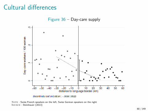
Cultural differences in labour supply
• Steinhauer (2013) ; Eugster et al. (2017)• Cultural differences could explain different labour supply
behaviour• Exploit the language difference with Switzerland between
German/French speakers• RDD along Rostigraben (i.e., rosti ditch or in French
barriere du rosti)
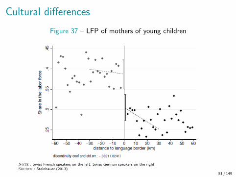
• Results• Little institutional difference• Working mothers more prevalent on the French-speaking
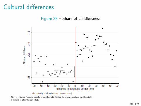
side of the language border• Share of childlessness more prevalent on the
German-speaking side
78 / 149

Cultural differences
Figure 35 – Map of Switzerland by language
Sources : Marco Zanoli ; Swiss Federal Statistical Office ; census of 2000
79 / 149
Cultural differences
Figure 36 – Day-care supply
Note : Swiss French speakers on the left, Swiss German speakers on the rightSource : Steinhauer (2013)
80 / 149
Cultural differences
Figure 37 – LFP of mothers of young children
Note : Swiss French speakers on the left, Swiss German speakers on the rightSource : Steinhauer (2013)
81 / 149
Cultural differences
Figure 38 – Share of childlessness
Note : Swiss French speakers on the left, Swiss German speakers on the rightSource : Steinhauer (2013)
82 / 149

III. Policy : Transfer to the poor
1 Traditional welfare
2 Optimal transfer policy
3 EITC/in-work tax credit
83 / 149

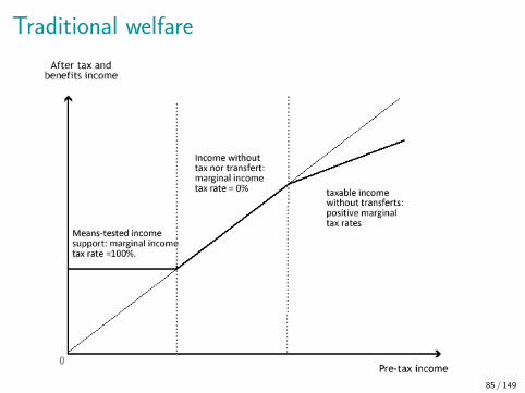
Traditional welfare
• Targeted benefits : tagging• Benefits on grounds of disability• Income support for the old• Income support for lone mothers
• Means-testing with 100% tax rate• Means-testing with 100% taper rate or 100% benefit
withdrawal (MTR of 100%)• Disregards for incentive effects• Creation of ‘poverty trap’ : once on welfare, no financial
incentives to go back to work
84 / 149
Traditional welfare
85 / 149
Negative income tax
• Negative income tax/basic income• Suggested by Milton Friedman (1962)• Replacement of all welfare benefits by a guaranteed income
paid by the government• Each additional dollar of income taxed at a marginal rate
below 100%• Basic income (BI) alternative description of NIT
• Large interest in NIT/BI, but no implementation• Randomized experience in the U.S. in the 1970s• Issue of unit of taxation (household vs individual)• Much larger cost than tagging to specific groups (or much
lower benefit)
86 / 149

Negative income tax
87 / 149

Iron triangle of redistribution
• Labour supply effects of NIT• Lower marginal tax rates for low incomes : positive effects
for the individuals not working• Higher marginal tax rates higher in the income
distribution : negative effects on labour supply
• The iron triangle of redistribution
1 Redistribution to the poor (high replacement income)2 Incentives to work (low marginal tax rates)3 Low cost to the government
88 / 149

Negative income tax
89 / 149

Negative income tax
90 / 149

Welfare to work
• Welfare reforms in the 1990s• “Welfare to work” or “workfare”• Removing high marginal tax rates on low incomes• Politically attractive to condition welfare on work
• Spread of these reforms• In the U.S., Earned Income Tax Credit (EITC)• In the U.K., Working Families Tax Credit (WFTC) and
then Working Tax Credit (WTC)• In France, Prime pour l’emploi (PPE) and Revenu de
solidarite active (RSA), then Prime d’activite• In Singapore, Workfare Income Supplement (WIS)
91 / 149

Tax credit
92 / 149
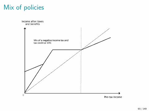
Mix of policies
93 / 149

Optimal transfer programmes
• Two approaches
1 Intensive margin : Mirrlees (1971)2 Extensive margin : Diamond (JPubE, 1980), Saez (QJE,
2002), Laroque (ECMA, 2005)
• Mirrlees model : negative income tax• Lump-sum grant −T (0) for those with no earnings• High MTR at the bottom :
a target transfers (low cost)b intensive response does not generate large losses (earnings
low at the bottom)
94 / 149

Optimal transfer programmes
• Diamond and Saez (JEP 2011)• g0 social marginal weight on zero earners• e0 elasticity of fraction non-working to the bottom
net-of-tax rate• Optimal bottom marginal tax rate with intensive margin
only
τ1 =g0 − 1
g0 − 1 + e0
• Implications of the formula• If society values redistribution towards zero earners, τ1 will
be highe.g., with g0 = 3, e0 = 0.5, then τ1 = 80%
95 / 149

Optimal transfer programmes
• Extensive margin responses• With fixed cost of work, extensive margin might be more
responsive• Empirical literature finds bigger labour supply elasticities at
the extensive margin
• Participation labour supply (Saez, QJE 2002)• Income when working ci = wi − Ti
• Income when not working c0
• Person works if ci − θ > c0, with θ fixed cost of work
96 / 149

Optimal transfer programmes
Figure 39 – Introducing in-work credit
Source : Piketty and Saez (2013), Fig. 8.
97 / 149

Optimal transfer programmes
• Results (extensive margin only)• Negative MTR are optimal (i.e., in-work credit are optimal)• NIT is not optimal
• Implications• In practice, both intensive and extensive margin exist• Trade-off between negative MTR in phase-in of in-work
credit (good for extensive margin) against high MTR inphase-out (bad for intensive margin)
98 / 149

The EITC in the US
• The Earned Income Tax Credit (EITC)• Large increase under Clinton administration• Now the largest cash antipoverty programme in the US
($34.6 billion in 2006)• EITC amounts depend on the number of children (higher
for families)• EITC is computed based on family income
• Three components
1 An increasing subsidy part (40% per dollar of wage top-up)2 A constant amount (no tax)3 Then a taper rate of 21% as benefits are withdrawn with
increasing income
99 / 149

The EITC in the US
Figure 40 – EITC schedule in 2016
100 / 149

The EITC in the US
101 / 149

Impact evaluation of EITC
• Impact on labour supply• Large empirical literature (Nichols and Rothstein, 2016)• Consistent positive employment effects for single mothers
i.e., $1000 increase in EITC leads to 6-7 pp increase inemployment
• Evidence of small intensive margin effects (e.g., clusteringat the kink)
⇒ Relatively successful redistribution programme
• Flaws of the programme• Low amount to the childless• Little increase with more than two children• Marriage penalty, complexity
102 / 149

Eissa and Liebman (QJE, 1996)
• First study on EITC• Early DiD approach• Compare single mothers (treated) with single women
without kids• Exploit the 1987 increase in EITC (TRA 1986)• Use CPS data
• Results• Positive impact on participation of lone mothers (+1.4-3.7
ppts)• No negative effects on married men’s labour supply• Modest reduction in married women’s labour supply
103 / 149

Eissa and Liebman (QJE, 1996)Table 5 – LFP rates of unmarried women
pre-TRA86 Post-TRA86 Diff. DiD
A. With vs. without childrenWomen with kids 0.729 0.753 0.024
(0.004) (0.004) (0.006)Women without kids 0.952 0.952 0.000 0.024
(0.001) (0.001) (0.002) (0.006)
B. Less than high-school – with vs. without childrenWomen with kids 0.479 0.497 0.018
(0.010) (0.010) (0.014)Women without kids 0.784 0.761 -0.023 0.041
(0.010) (0.009) (0.013) (0.019)
C. High-school – with vs. without childrenWomen with kids 0.764 0.787 0.023
(0.006) (0.006) (0.008)Women without kids 0.945 0.943 -0.002 0.025
(0.002) (0.003) (0.004) (0.009)
Source : Eissa and Liebman (1996), Tab. II, p. 617.104 / 149

Hoynes and Patel (JHR, 2017)
• Recent study on EITC• Exploit the 1994-95 increase in EITC (OBRA 1993)• Use CPS March data• DiD + parametrized DiD + event study
• Event study approach• Estimating full set of year effets, idem for treated
yit = α+T∑t0
βj [I (t = j)xtreatc ]+ηst+γc+ΦXit+γZcst+εit
• treatc is dummy for number of children (treatment group)• βj difference between treatment and control in each year j• ηst state × year fixed effects• Zcst state × year × nber children unemployment rates
105 / 149

1993 EITC expansion
Figure 41 – Maximum benefits by number of children
Source : Hoynes and Patel, 2017
106 / 149

Hoynes and Patel (JHR, 2017)
Figure 42 – Estimates of the Effects of OBRA1993 on Employment
Source : Hoynes and Patel (2017), Fig. 6
107 / 149
Hoynes and Patel (JHR, 2017)
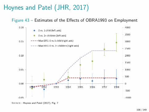
Figure 43 – Estimates of the Effects of OBRA1993 on Employment
Source : Hoynes and Patel (2017), Fig. 7
108 / 149
Hoynes and Patel (JHR, 2017)
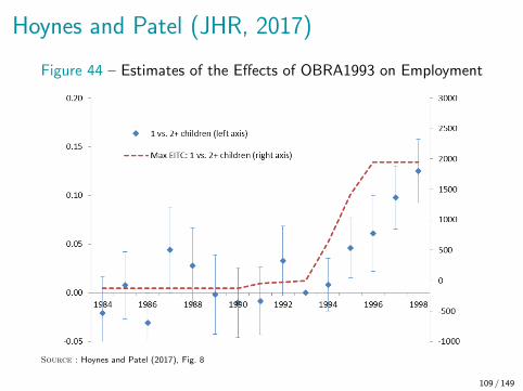
Figure 44 – Estimates of the Effects of OBRA1993 on Employment
Source : Hoynes and Patel (2017), Fig. 8
109 / 149

Hoynes and Patel (JHR, 2017)
Figure 45 – Estimates of the Effects of OBRA1993 on Poverty(above 100% of Poverty Threshold)
Source : Hoynes and Patel (2017). 110 / 149

Hoynes and Patel (JHR, 2017)
Figure 46 – Estimates of the Effects of OBRA1993 on Incomeabove poverty level
Source : Hoynes and Patel (2017).111 / 149
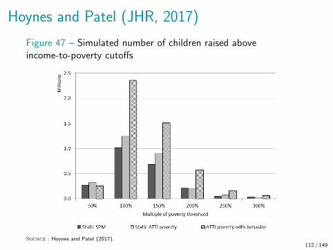
Hoynes and Patel (JHR, 2017)
Figure 47 – Simulated number of children raised aboveincome-to-poverty cutoffs
Source : Hoynes and Patel (2017).112 / 149

Hoynes and Patel (JHR, 2017)
• Results• $1000 increase in policy-induced increase in the EITC leads
to a 5.6-7.8 percentage point increase in employment forsingle mothers
• Extensive margin elasticities range from 0.32-0.45• Ignoring the behavioural response leads to an
underestimate of the anti-poverty effects by 50 percent
113 / 149

Bunching at kinks
• Saez (AEJ-EP, 2010)• Key prediction of standard labour supply model : individuals
should bunch at (convex) kink points of the budget set• Amount of bunching at kinks provides non-parametric
estimates of intensive elasticity
• Formula for elasticity
εc =dz/z
dt/(1− t)=
excess mass at kink
% change in net of tax rate
114 / 149
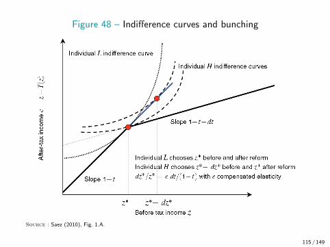
Figure 48 – Indifference curves and bunching
Source : Saez (2010), Fig. 1.A.
115 / 149
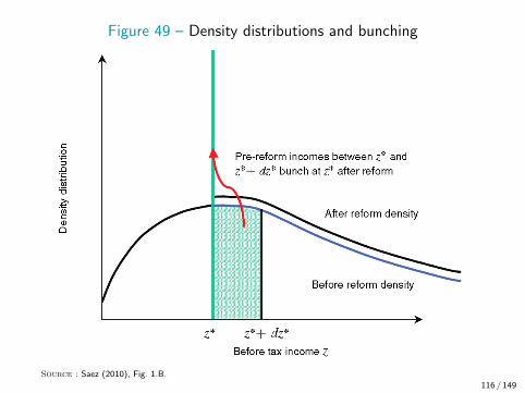
Figure 49 – Density distributions and bunching
Source : Saez (2010), Fig. 1.B.
116 / 149

Figure 50 – Estimating excess bunching using empirical densities
Source : Saez (2010), Fig. 2
117 / 149

Saez (AEJ-EP, 2010)
• Some evidence of bunching at EITC• Evidence of bunching at first kink point of EITC⇒ implied elasticity of 0.25
• Mechanisms for bunching• Self-employment income for EITC
118 / 149
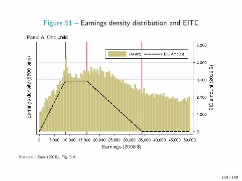
Figure 51 – Earnings density distribution and EITC
Source : Saez (2010), Fig. 3.A.
119 / 149

Figure 52 – Earnings density distribution and EITC
Source : Saez (2010), Fig. 3.B.
120 / 149

Figure 53 – Earnings density distribution : wage earners vsself-employed
Source : Saez (2010), Fig. 4.A.
121 / 149

Figure 54 – Earnings density distribution : wage earners vsself-employed
Source : Saez (2010), Fig. 4.B.
122 / 149

Chetty, Friedman, Saez (AER, 2013)
• Exploit heterogeneous information about EITC• Use U.S. population wide tax return data 1996-2009• Measure heterogeneity in bunching of self-employed across
3-digit zip codes• Idea is to proxy for local information with bunching
• Main empirical approaches• Estimate impact on earnings of moving to high bunching
area• Estimate impact on earnings of child birth in high bunching
area compared to low bunching area• Identification using low bunching area as counterfactual
123 / 149

Figure 55 – Earnings distribution in Kansas
Source : Chetty, Friedman and Saez (2013).
124 / 149

Figure 56 – Earnings distribution in Texas
Source : Chetty, Friedman and Saez (2013).
125 / 149
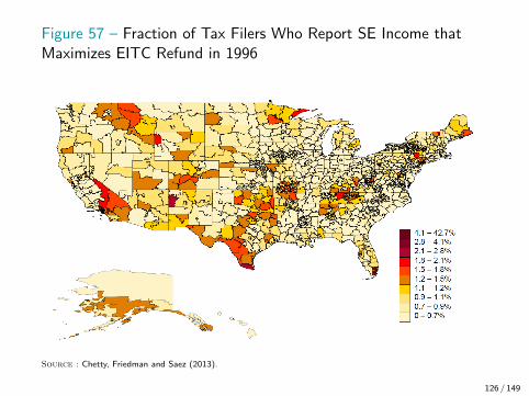
Figure 57 – Fraction of Tax Filers Who Report SE Income thatMaximizes EITC Refund in 1996
Source : Chetty, Friedman and Saez (2013).
126 / 149

Figure 58 – Fraction of Tax Filers Who Report SE Income thatMaximizes EITC Refund in 2002
Source : Chetty, Friedman and Saez (2013).
127 / 149

Figure 59 – Fraction of Tax Filers Who Report SE Income thatMaximizes EITC Refund in 2005
Source : Chetty, Friedman and Saez (2013).
128 / 149

Figure 60 – Fraction of Tax Filers Who Report SE Income thatMaximizes EITC Refund in 2008
Source : Chetty, Friedman and Saez (2013).
129 / 149

Figure 61 – Event Study of Sharp Bunching Around Moves
Source : Chetty, Friedman and Saez (2013).
130 / 149

Figure 62 – Change in EITC Refunds vs. Change in SharpBunching for Movers
Source : Chetty, Friedman and Saez (2013).
131 / 149

Figure 63 – Income Distribution For Single Wage Earners with OneChild High vs. Low Bunching Areas
Source : Chetty, Friedman and Saez (2013).
132 / 149

Figure 64 – Difference in Wage Earnings Distributions BetweenTop and Bunching Decile Wage Earners with One Child
Source : Chetty, Friedman and Saez (2013).
133 / 149

Figure 65 – Difference in Wage Earnings Distributions BetweenTop and Bunching Decile Wage Earners with One Child
Source : Chetty, Friedman and Saez (2013).
134 / 149

Figure 66 – Earnings Distribution in the Year Before First ChildBirth for Wage Earners
Source : Chetty, Friedman and Saez (2013).
135 / 149

Figure 67 – Earnings Distribution in the Year of First Child Birthfor Wage Earners
Source : Chetty, Friedman and Saez (2013).
136 / 149

Chetty, Friedman, Saez (AER, 2013)
Table 6 – Elasticity Estimates Based on Change in EITCRefunds Around Birth of First Child
Mean Phase-in Phase-out Extensiveelasticity elasticity elasticity elasticity
A. Wage earningsElasticity in U.S. 2000-05 0.21 0.31 0.14 0.19
(0.012) (0.018) (0.015) (0.019)Elasticity in top decile ZIP-3s 0.55 0.84 0.29 0.60
(0.020) (0.031) (0.020) (0.034)
B. Total earnings (including self-employment income)Elasticity in U.S. 2000-05 0.36 0.65 0.36
(0.017) (0.030) (0.019)Elasticity in top decile ZIP-3s 1.06 1.70 0.31 1.06
(0.029) (0.047) (0.010) (0.040)
Source : Chetty, Friedman and Saez (2013), Tab. 3.
137 / 149

Chetty, Friedman, Saez (AER, 2013)• Findings
• Places with high self-employment EITC bunching displaywage earnings distribution more concentrated aroundplateau
• Significant intensive margin effects larger than extensivemargin effects
• Interpretation and question• Extensive margin effect could come from imperfect
knowledge about the schedule of EITC (salience effect)• Among SE, bunching could be reporting not real economic
activity
• General lesson : knowledge of policy is key• key explanatory variable in estimation of behavioural
responses• Information is a powerful and inexpensive policy tool to
affect behaviour 138 / 149

Kleven (2020) : challenging the consensus• The consensus
• Extensive margin is sizeable, and justifies programmes likethe EITC (WFTC, Prime d’activite, etc.)
• Consensus originates from– labour supply literature (Heckman, 1993)– macro literature (Rogerson, 1988)– evaluation of EITC (Eissa and Liebman, 1996)
• Kleven’s Reappraisal• The consensus view on the EITC and the extensive margin
is fragile at best• Only one period in the U.S. leads to strong effects (OBRA
93)• Strong responses from individuals not affected by EITC
(with 3+ kids)• Other countries have found much smaller effects, e.g., UK
(Brewer et al. 2005)139 / 149
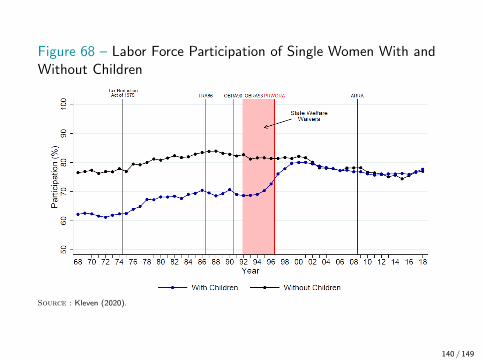
Figure 68 – Labor Force Participation of Single Women With andWithout Children
Source : Kleven (2020).
140 / 149

Figure 69 – Employment of Single Women : DiD by Number ofChildren
Source : Kleven (2020).
141 / 149

Figure 70 – Stacked Event Studies : Single Women With vs.Without Children
Source : Kleven (2020).
142 / 149

Kleven (2020) : challenging the consensus
• Explaining the large increase in employment of U.S.single mothers• No question that employment of US single mothers
dramatically increased in one short period of time• States welfare reform (e.g., time limits, work requirements,
training and job search activities)• Strong economy
• Behavioural issues• EITC not very well known• Welfare reform was very salient• Welfare culture (“undeserving poor”, etc.)
143 / 149

References– Alesina, A., Glaeser, E. and Sacerdote, B. (2005), “Work and Leisure in the United States and Europe : Why
So Different ?” NBER Macroeconomics Annual 20, pp. 1–64.
– Anderson, P. and Meyer, B. (2000), “The Effects of the Unemployment Insurance Payroll Tax on Wages,Employment, Claims and Denials”, Journal of Public Economics, 78 (1-2) : 81-106.
– Ashenfelter, O., and Plant, M. (1990), “Nonparametric Estimates of the Labor-Supply Effects of NegativeIncome Tax Programs”, Journal of Labor Economics 8 (1), pp. S396-415.
– Azmat, G. (2019) “Incidence, Salience and Spillovers : The Direct and Indirect Effects of Tax Credits onWages”, Quantitative Economics, vol. 10 (1), pp. 239–273.
– Bianchi, M., Gudmundsson, B. and Zoega, G. (2001) “Iceland’s Natural Experiment in Supply-SideEconomics”, The American Economic Review 91 (5), pp. 1564-79.
– Bingley, P. and Lanot, G. (2002), “The Incidence of Income Tax on Wages and Labour Supply”, Journal ofPublic Economics 83 (2), pp. 173–194.
– Blanchard, O. (2004), “The Economic Future of Europe”, The Journal of Economic Perspectives 18 (4),pp. 3–26.
– Blau, F. and Kahn, L. (2003), “Changes in the Labor Supply Behavior of Married Women : 1980-2000”,Journal of Labor Economics, 25 (3), pp. 393–438.
– Blundell, R., Bozio, A. and Laroque, G. (2011) “Labor Supply and the Extensive Margin”, The AmericanEconomic Review 101 (3), pp. 482–86.
– Blundell, R., Bozio, A. and Laroque, G. (2013) “Extensive and Intensive Margins of Labour Supply : Work andWorking Hours in the US, the UK and France”, Fiscal Studies 34 (1) : pp. 1–29.
– Blundell, R. and MaCurdy, T. (1999), “Labour Supply : A Review of Alternative Approaches”, in Ashenfelterand Card (eds), Handbook of Labour Economics, Elsevier North Holland.
– Brewer, M., Duncan, A., Shephard, A. and Suarez, M. J. (2005), “Did Working Families’ Tax Credit work ?The final evaluation of the impact of in-work support on parents’ labour supply and take-up behaviour in theUK”, HMRC working paper no. 2.
– Brewer, M., Duncan, A., Shephard, A. and Suarez, M. J. (2006), “Did the Working Families Tax Creditwork ?”, Labour Economics, Vol. 13, No 6, pp. 699-720.
– Brittain, J. (1971), “The Incidence of Social Security Payroll Taxes”. The American Economic Review 61 (1) :110-125.
– Bozio, A., Breda, T. and Julien Grenet, G. (2019) “Does Tax-Benefit Linkage Matter for the Incidence ofSocial Security Contributions ?”, PSE working paper 1943, IZA DP No. 12502.
144 / 149

References– Blundell, R. (2006), “Earned income tax credit policies : Impact and Optimality”, The 2005 Adam Smith
Lecture, Labour Economics, Vol. 13, pp. 423-443.
– Chetty, R. (2009), “Is the Taxable Income Elasticity Sufficient to Calculate Deadweight Loss ? TheImplications of Evasion and Avoidance’. American Economic Journal : Economic Policy 1 (2) : 31-52.
– Chetty, R. (2012), “Bounds on Elasticities with Optimization Frictions : A Synthesis of Micro and MacroEvidence on Labor Supply’. Econometrica 80 (3) : 969-1018.
– Chetty, R., Friedman, J. and Saez, E. (2013) “Using Differences in Knowledge Across Neighborhoods toUncover the Impacts of the EITC on Earnings”, The American Economic Review 103 (7) : 2683–2721.
– Chetty, R. and Saez, E. (2008) “Information and Behavioral Responses to Taxation : Evidence from anExperiment with EITC Clients at H&R Block’. UC-Berkeley Mimeo.
– Chetty, R., Friedman, J., Olsen, T. and Pistaferri, L. (2011) “Adjustment Costs, Firm Responses, and Microvs. Macro Labor Supply Elasticities : Evidence from Danish Tax Records’. The Quarterly Journal of Economics126 (2) : 749-804.
– Chetty, R., Guren, A., Manoli, D. and Weber, A. (2011), “Are Micro and Macro Labor Supply ElasticitiesConsistent ? A Review of Evidence on the Intensive and Extensive Margins”, The American Economic Review101 (3), pp. 471–75.
– Delalande, N. (2011), Les Batailles de L’impot. Consentement et Resistances de 1789 a nos jours. L’universHistorique. Paris : Seuil.
– Delalande, N., and Spire, A. (2010), Histoire Sociale de L’impot. Reperes. Paris : La Decouverte.
– Eissa N. and Liebman J. (1996), “Labor Supply Response to the Earned Income Tax Credit”, QuarterlyJournal of Economics, Vol. 111, No 2, pp. 605-637.
– Eissa, N., Kleven, H. and Kreiner, C. (2008) “Evaluation of Four Tax Reforms in the United States : LaborSupply and Welfare Effects for Single Mothers” Journal of Public Economics 92 (3-4) : 795-816.
– Eugster, B., Lalive, R., Steinhauer, A. and Zweimuller, J. (2017) “Culture, Work Attitudes, and Job Search :Evidence from the Swiss Language Border”, Journal of the European Economic Association, Volume 15, Issue5, pp. 1056–1100.
– Fack, G. (2006), “Are Housing Benefit an Effective Way to Redistribute Income ? Evidence from a NaturalExperiment in France”, Labour Economics, 13 (6), pp. 747–71.
145 / 149
References
– Fehr, Ernst, and Lorenz Goette. 2007. “Do Workers Work More If Wages Are High ? Evidence from aRandomized Field Experiment’. The American Economic Review 97 (1) : 298-317.
– Guery, A. (1986), “Etat, classification sociale et compromis sous Louis XIV : la capitation de 1695”. Annales,41 (5) : 1041-60.
– Gruber, J. (1997) “The Incidence of Payroll Taxation : Evidence from Chile”. Journal of Labor Economics 15(S3) : S72-101.
– Hamermesh, D. (1979), “New Estimates of the Incidence of the Payroll Tax”. Southern Economic Journal 45(4) : 1208.
– Holmlund, B. (1983), “Payroll Taxes and Wage Inflation : The Swedish Experience”. The ScandinavianJournal of Economics, 1-15.
– Hoynes, H. and Patel, A. (2017) “Effective Policy for Reducing Poverty and Inequality ? The Earned IncomeTax Credit and the Distribution of Income”, Journal of Human Resources, 1115-7494R1.
– Imbens, Guido W., Donald B. Rubin, and Bruce I. Sacerdote (2001), “Estimating the Effect of UnearnedIncome on Labor Earnings, Savings, and Consumption : Evidence from a Survey of Lottery Players’. TheAmerican Economic Review 91 (4), pp 778–94.
– Keane, M., and Rogerson, R. (2012), “Micro and Macro Labor Supply Elasticities : A Reassessment ofConventional Wisdom’. Journal of Economic Literature 50 (2), pp. 464–76.
– Ketterle, J. (1994), Die Einkommensteuer in Deutschland, Modernisierung und Anpassung einer direktenSteuer von 1890-91 bis 1920, Botermann & Botermann Verlag, Cologne.
– Kleven, H. (2020) “The EITC and the Extensive Margin : A Reappraisal”, NBER Working Paper No. 26405,February 2020.
– Korkeamaki, Ossi, and Roope Uusitalo (2009), “Employment and Wage Effects of a Payroll-Tax Cut-evidencefrom a Regional Experiment’. International Tax and Public Finance 16 (6) : 753-72.
146 / 149

References– Kubik, J. (2004), “The Incidence of Personal Income Taxation : Evidence from the Tax Reform Act of 1986”.
Journal of Public Economics 88 (7-8) : 1567-88.
– Lehmann, E., Marical, F. and Rioux, L. (2013), “Labor Income Responds Differently to Income-Tax andPayroll-Tax Reforms’. Journal of Public Economics 99 : 66-84.
– Ljungqvist, L., Sargent, T., Blanchard, O. and Prescott, E. (2006), “Do Taxes Explain EuropeanEmployment ? Indivisible Labor, Human Capital, Lotteries, and Savings [with Comments and Discussion]’.NBER Macroeconomics Annual 21 : 181-246.
– Maag, E., Steuerle, E., Chakravarti, C., and Quakenbush, C. (NTJ, 2012) “How Marginal Tax Rates AffectFamilies at Various Levels of Poverty”, National Tax Journal, vol. 65(4), pp. 759–782.
– Mehrotra, A. (2013), Making the Modern American Fiscal State. Law, Politics, and the Rise of ProgressiveTaxation, 1877-1929, Cambridge University Press.
– Neubig, T. (1981), “The Social Security Payroll Tax on Wage Growth’. National Tax Association, 196-201.
– Neurisse, A. (1996), Histoire de La Fiscalite En France. Paris : Economica.
– Munnell, A. (1986), Lessons from the Income Maintenance Experiments : Proceedings of a Conference Held atMelvin Village, New Hampshire. Federal Reserve Bank of Boston & The Brookings Institution.
– Saez, E. (2002), “Optimal Income Transfer Programs : Intensive Versus Extensive Labor Supply Responses”,Quarterly Journal of Economics, Vol. 117, No. 3, pp. 1039-1073.
– OECD (1990), “Employment Outlook”.
– Ohanian, L. and Raffo, A. (2012), “Aggregate Hours Worked in OECD Countries : New Measurement andImplications for Business Cycles’. Journal of Monetary Economics, 59 (1) : 40-56.
– Ohanian, L., A. Raffo, and Rogerson, R. (2008), “Long-Term Changes in Labor Supply and Taxes : Evidencefrom OECD Countries, 1956-2004’. Journal of Monetary Economics 55 (8) : 1353-62.
– Ooghe, Erwin, Erik Schokkaert, and Jef Flechet. 2003. “The Incidence of Social Security Contributions : AnEmpirical Analysis’. Empirica 30 (2) : 81-106.
– Piketty, T. (2001), Les Hauts Revenus En France Au XXe Siecle. Inegalites et Redistributions 1901-1998.Grasset & Fasquelle.
– Piketty, T. (2013), Le Capital Au XXIe Siecle. Seuil.
– Prescott, E. (2004), “Why Do Americans Work so Much More than Europeans ?’ Quarterly Review, no. Jul :2-13.
147 / 149

References
– Prescott, Edward C. 2006. “Nobel Lecture : The Transformation of Macroeconomic Policy and Research’.Journal of Political Economy 114 (2) : 203-35.
– Ramey, Valerie A., and Neville Francis. 2009. “A Century of Work and Leisure’. American Economic Journal :Macroeconomics 1 (2) : 189-224.
– Rees, A. (1974), “An Overview of the Labor-Supply Results’. The Journal of Human Resources 9 (2) : 158-80.
– Rogerson, R. (1988), “Indivisible Labor, Lotteries and Equilibrium’. Journal of Monetary Economics 21 (1) :3-16.
– Rogerson, R. (2007), “Taxation and Market Work : Is Scandinavia an Outlier ?’ Economic Theory 32 (1) :59-85.
– Rothstein, Jesse. 2010. “Is the EITC as Good as an NIT ? Conditional Cash Transfers and Tax Incidence’.American Economic Journal : Economic Policy 2 (1) : 177-208.
– Saez, E 2010. “Do Taxpayers Bunch at Kink Points ?’ American Economic Journal : Economic Policy 2 (3) :180-212.
– Saez, E., Matsaganis, M. and Tsakloglou, P. (2012), “Earnings Determination and Taxes : Evidence From aCohort-Based Payroll Tax Reform in Greece”, The Quarterly Journal of Economics 127 (1), pp. 493–533.
– Saez, E., Schoefer, B. and Seim, D. (2019) “Payroll Taxes, Firm Behavior, and Rent Sharing : Evidence from aYoung Workers’ Tax Cut in Sweden” American Economic Review Vol. 109, No. 5, pp. 1717-63.
– Steinhauer, Andreas. 2013. “Identity, Working Moms, and Childlessness : Evidence from Switzerland’.University of Zurich Discussion Paper.
– Touzery, M. (1994), L’invention de l’impot sur le revenu – La taille tarifee 1715-1789, Institut de la gestionpublique et du developpement economique, Comite pour l’histoire economique et financiere de la France.
– Witte, J. (1985), The Politics and Development of the Federal Income Tax, University of Wisconsin Press.
148 / 149

Definitions
Average tax rate τ is the proportion of income R leading totax T
τ =T
R
Marginal tax rate µ is the share of tax on additional unit ofincome
µ =∂T
∂R
Progressivity A tax schedule is said progressive if the averagetax rate is increasing with income
Regressivity A tax schedule is said progressive if the averagetax rate is increasing with income
149 / 149