Measurement 1

Pauline Charousset Denis Cogneau Julien Grenet

LecturesWhen: 10-sept

Intro 1 15-sept group116-sept 18-sept group2Intro 2

29-sept group101-oct 02-oct group2Health08-octGDP 13-oct group1

15-oct 16-oct group2PricesBreak

29-octPoverty 03-nov group105-nov 06-nov group2

Inequality12-nov

Inequality 17-nov group119/20-nov 20-nov group2

Employment

01-déc group103-déc 04-déc group2

EducationBreak

06-jan weekEXAM

Who: DCJG

Tutorials

PC

Validation Attendance at lectures and tutorials are compulsory Punctuality is required 50% of grade from homework assignments average - 6 hwks, 3 randomly selected are graded - (Same hwk number for each student, for equity reasons) - Lottery: stratified by 1-2 / 3-4 / 5-6 feedback at each step - Hwk not handed or handed too late = 0 50% from 3-hours written exam in January 6, 7 or 8 Corrected last-year exam will be provided; usually: - Quizz: 12 MCQs for 6 pts (no penalty for wrongs) - 2 short questions on lectures contents (2-3 pts each) - 2 problems (5-6 pts each)

Today

• Empirical evidence and common sense • Big data? Or new & good data (analysis)? • Social facts are constructs • Factual ≠ Counterfactual • 4 pillars of measurement: D, A, Q, S • D: Definition • A: Axiomatics

Next week

• Q: Quality – Measurement errors

• S: Sampling – Probabilitic samples vs. censuses – Law of large numbers – Central Limit theorem – Two-stages samples – Stratification

Empirical « Evidence » (1) Large surveys of attitudes of American soldiers during WW2, published in 1949, in four volumes, by Paul Lazarsfeld & team. Arthur Schlesinger, Harvard historian, in The Partisan Review: « ponderous demonstration in Newspeak of such facts like this: (…) married privates are more likely than single privates to worry about their families back home. » Other results underlined by Lazarsfeld: 1. Better educated soldiers suffered more adjustment problems than less educated

soldiers. (Intellectuals less prepared for battle stresses than street-smart people.) 2. Southern soldiers coped better with the hot South Sea Island climate than Northern soldiers. (Southerners are more accustomed to hot weather.) 3. White privates were more eager to be promoted to noncommissioned officers than Black privates. (Years of oppression take a toll on achievement motivation.) 4. Southern Blacks preferred Southern to Northern White officers. (Because Southern officers were more experienced and skilled in interacting with Blacks). 5. As long as the fighting continued, soldiers were more eager to return home than after the war ended. (During the fighting, soldiers knew they were in mortal danger.)

Empirical « Evidence » (2) Evidence = Obviousness ? Actually the results were exactly the opposite: Paul F. Lazarsfeld, 1949. “The American Soldier-An Expository Review”, The Public Opinion Quarterly, 13(3): pp. 377-404 (http://www.derekchristensen.com/5-truths-that-hindsight-made-clear/) Anything seems commonplace, once explained. – Dr. Watson to Sherlock Holmes “Common sense” is not of great guidance Said in another words: “Theory” can explain almost everything Or at least: there is more available theories than facts

Innovative data, big data • Micro-datasets from surveys on the Web • Long-term panels following cohorts • Exhaustive administrative data, censuses • Digitized historical archives, libraries + OCR • Mobile phones and Internet data, sensor data • Remote sensing satellite imagery Good… but also risks of misuse See e.g. Big data is not about the data! Gary King, Harvard U. It’s rather about progresses in data construction and analytics.

Google books

Ravallion 2011

Short term growth: Indonesian crisis in Java

Remote sensing images: note the dark areas in 1975

First map : Geographers in 1960s Second map: Based on SPOT satellite images

Côte d’Ivoire 1965-69 2000-04

Constructing “social facts” (1) • “Fact”: should not require an inter-subjective

agreement (or a poll) to be “true” – truth is conditional to a method or procedure of data collection and aggregation: this procedure can be liked or not, anyway the procedural link between the data and the fact remains

Ex.: Food price ≠ Tasty character of a given food product • “Social”: we are not talking of facts that are

particular to an individual or to very small groups of individuals

(Durkheim did not talk about suicide as a personal distress but as a widespread and regular phenomenon and as a social symptom)

Constructing social facts (2) Social facts are counts, even in

anthropology: e.g. “prohibition of incest is universal”,… or “this group has a very peculiar mythology” (i.e. as ≠ from other groups)

The problem is not quantitative vs. qualitative, it’s

bad quality quantitative. Or not letting the machine control human thinking…

Constructing social facts (3)

A social fact is a construct depending on a methodology of accounting that has 4 components:

1. What is to be measured? Definition 2. What is to be computed? Axiomatics 3. How to measure variables? Quality control 4. How to count individuals? Sampling

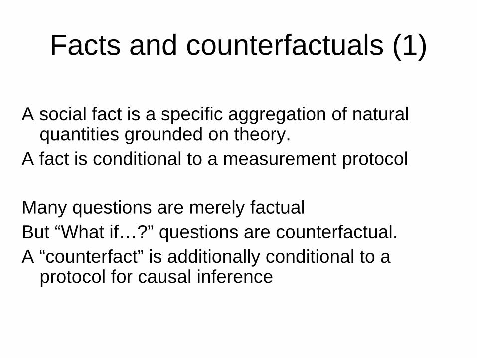
Facts and counterfactuals (1) A social fact is a specific aggregation of natural

quantities grounded on theory. A fact is conditional to a measurement protocol Many questions are merely factual But “What if…?” questions are counterfactual. A “counterfact” is additionally conditional to a

protocol for causal inference

Facts and counterfactuals (2) - Do richer people have taller children? - When income increases, do children grow taller as a

consequence? - Do income differentials between social origins represent

a large share of total income inequality in Brazil? - What income inequality would be observed if social

mobility was improved thanks to educational programs?

Facts and counterfactuals (3) Facts are often too quickly interpreted as

counterfactuals, especially when they produce a rich description, for instance through decomposition techniques (for growth, inequality, mobility, etc.)

Facts rule out some theories that cannot

account for them; but they are compatible with many others.

Constructing social facts (end)

1. What is to be measured? Definition D. 2. What is to be computed? Axiomatics A. 3. How to measure variables? Quality Q. 4. How to count individuals? Sampling S.

Table example: Siege of Paris 1870-71 Table 1. Variations of mortality quotients for the 1866-72 birth cohorts

Mortality quotients

(%) Pre-crisis 1866 1867 1868 1869 1870 1871 1872

1q0 25.2 25.2 25.2 25.2 25.2 36.5 32.2 24.1

4q1 16.5 17.1 19.8 25.1 32.0 17.5 14.4 16.5

5q0 37.5 38.0 40.0 44.0 49.2 47.6 42.0 36.6

Source: Vital records of the 19th district.

Coverage: Deaths of men below 20 year-old in the 19th district.

Notes: Construction of the benchmark pre-crisis estimate (see also appendix A1): For infant mortality (1q0), we use recorded deaths before age 1 and between

September 1869 and August 1870 for the 4-month cohort born in Paris between Sept. and Dec. 1869; we complement our estimate using recorded deaths before age 1 in

the same months of 1869 (Sept. to Dec.), using the cohort born between Sept. and Dec. 1868. For the next mortality quotient (1q1), we similarly use recorded deaths

between ages 1 and 2, and between September 1869 and August 1870 for the 4-month cohort born between September and December 1868. Once again, we use the

preceding cohort (Sept. to Dec. 1867) to complete our estimate. For years before 1868, we compute an estimate of the 4-month cohorts' sizes by applying the average of

the shares for 1868 and 1869 to the total number of births. We assume that the benchmark estimate for 1q0 applies. For 1q2 and 1q3 we repeat the same procedure.

D.: Mortality risks in case of famine (their variation with age at the time) A.: Mortality quotients are the best variable (rather than # of deaths) – (Fertility also varied) Q.: Explained in footnotes S.: Explained in footnotes – Migration concern: adressed in the text

1 – Definition (a) Concepts are derived from theory: - of growth, international economics - of development - of justice - of social integration - etc. Before to be measured, concepts should be made

precise in terms of population covered and dimensions concerned: …

1- Definition (b) “Theory” should define the concepts to be measured: - national wealth: non-market activities, waste of natural

resources? - access to goods: is it income or consumption? full time

income? income per adult equivalent? - poverty: do differences between the poor matter? - income inequality: relative or absolute income

differences? - inequality in health: does it matter per se or only its

correlation with other inequalities? - unemployment or migration: voluntary vs. involuntary,

transient vs. permanent - trade openness: trade intra-firms ≠ extra-firms? - education: market returns or cognitive achievements?

Empirical Evidence again (3) Durkheim study on Suicide published in 1897 Baudelot & Establet repeat the study in 1984 1. Men commit suicide more than Women? 2. Urban more than Rural? 3. More on Monday or on Sunday? 4. More in Winter or in Spring or Summer? 5. More in daylight or at night?

Émile Durkheim,1897. Le Suicide : Étude de sociologie. Paris: Félix Alcan Chistian Baudelot, Robert Establet, 1984. “Suicide : l'évolution séculaire d'un fait social.” Economie et Statistique 168(1): 59-70. Same authors: Suicide. L'envers de notre monde, Seuil, 2006. Durkheim et le suicide, PUF, 2011.

Empirical Evidence again (4) 1. Men more than Women, at any age and

whatever marital status 2. Urban more than Rural today Urban in 19th c., Rural in 20th 3. More on Monday 4. More in Spring, June, September 5. More in daylight Failed suicide attempts ≠ deaths by suicide Definition matters!

2 - Axiomatics Quantities observed in “nature”: price of Big Mac,

quantity of rice, height stature, number of people in a place at a time…

[May depend on who observes: measure problem]

Measuring concepts requires an aggregation of “natural quantities”:

- in the space of variables: cost of living, agricultural production, individual income… literacy…

- in the space of individuals: mean income, stunting / overweight, poverty, inequality…

2- Ex.: Axioms for inequality indexes

Identical individuals (in needs), heterogenous in income

Axiom 1: Inequality should decrease when transferring income from a rich to a poor

(Variance of logarithms: no; Gini: yes) Axiom 2a: Inequality is unchanged if all incomes are

doubled (Gini) Axiom 2b: Inequality is unchanged if a given amount is

added to all incomes (Gini index not divided by the mean)

At date t; n individuals indexed by i (or j); income yi(t); mean income μy(t)

• Traditional “relative” Gini: G = 1/(2n²μy(t)) Σi Σj | yi(t) – yj(t) | • “Absolute” Gini: Abs-G = 1/(2n²) Σi Σj | yi(t)– yj(t) | [ In the figure divided by 1992 median, i.e. a time-invariant

factor, just for normalization]

Getting it all wrong Ex. Samuel Morton’s measurement of skulls (1849) – ‘sample’ of 623 skulls: caucasians, indians, asians,

africans… - D.: skull volume related to « intelligence » - WRONG - A.: no correction for body stature - WRONG - Q.: use seeds rather than metal balls, selective heaping -

WRONG - S.: huge sampling bias, subjective selection, no

confidence intervals – WRONG

See Stephen J. Gould, 1996, The Mismeasure of Man, Norton

Measurement 2

3 – Quality Ex-ante: How to ask questions in a census or a survey: formulation,

order, items… Should one rely on self-declarations? On interviewer

observation? When to use direct measurements: literacy, health? How to mimic real life: buying products to know prices,

making real exams? How to reach the underground : informal trade flows,

unregistered economy, capital flight? How to avoid refusals to answer? Ex-post: How to deal with measurement errors?

3- Measurement errors “Classical” = white noise [Non-classical: correlated with the true value; for ex., bounded variables like dummies] 𝑌 = 𝑌∗ + 𝑢 𝐸(𝑢) = 0 𝐶𝐶𝐶 𝑢,𝑌∗ = 𝐸 𝑢𝑌∗ = 0 𝑌 = measured value 𝑌∗ = “true” value 𝑢 = measurement error Increases variance: 𝑉(𝑌) = 𝑉(𝑌∗) + 𝑉(𝑢) = 𝑉(𝑌∗). (1 + 𝜃) 𝜃 = 𝑉(𝑢)

𝑉(𝑌∗)> 0 = Noise-to-signal ratio

Hence enhances the “impression” of inequality Administrative data and self-declared data on income compared: θ ≈ 20-30% in the US (cf. Handbook of Econometrics vol.5, Measurement errors in survey data)

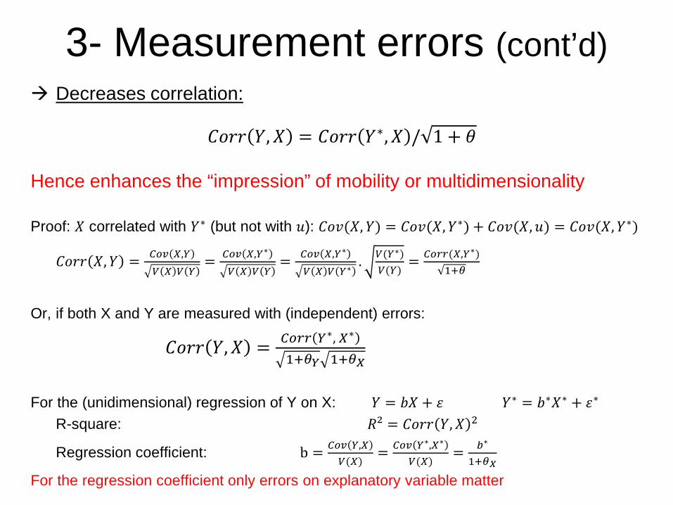
Decreases correlation:

𝐶𝐶𝐶𝐶 𝑌,𝑋 = 𝐶𝐶𝐶𝐶 𝑌∗,𝑋 / 1 + 𝜃 Hence enhances the “impression” of mobility or multidimensionality Proof: 𝑋 correlated with 𝑌∗ (but not with 𝑢): 𝐶𝐶𝐶(𝑋,𝑌) = 𝐶𝐶𝐶(𝑋,𝑌∗) + 𝐶𝐶𝐶(𝑋,𝑢) = 𝐶𝐶𝐶(𝑋,𝑌∗)

𝐶𝐶𝐶𝐶 𝑋,𝑌 = 𝐶𝐶𝐶 𝑋,𝑌𝑉 𝑋 𝑉 𝑌

= 𝐶𝐶𝐶 𝑋,𝑌∗

𝑉 𝑋 𝑉 𝑌= 𝐶𝐶𝐶 𝑋,𝑌∗

𝑉 𝑋 𝑉 𝑌∗. 𝑉(𝑌∗)

𝑉(𝑌)= 𝐶𝐶𝐶𝐶(𝑋,𝑌∗)

1+𝜃

Or, if both X and Y are measured with (independent) errors:

𝐶𝐶𝐶𝐶 𝑌,𝑋 = 𝐶𝐶𝐶𝐶 𝑌∗, 𝑋∗

1+𝜃𝑌 1+𝜃𝑋

For the (unidimensional) regression of Y on X: 𝑌 = 𝑏𝑋 + 𝜀 𝑌∗ = 𝑏∗𝑋∗ + 𝜀∗ R-square: 𝑅𝑅 = 𝐶𝐶𝐶𝐶 𝑌,𝑋 2

Regression coefficient: b = 𝐶𝐶𝐶 𝑌,𝑋𝑉(𝑋)

= 𝐶𝐶𝐶 𝑌∗,𝑋∗

𝑉(𝑋)= 𝑏∗

1+𝜃𝑋

For the regression coefficient only errors on explanatory variable matter

3- Measurement errors (cont’d)

2 measurements 𝑌 and 𝑌′ taken on the same sample. (For ex., think of two height stature measurements for the same individual at the same time)

Let’s compute the average of the two individual measurements: 𝑀𝑌 = (𝑌 + 𝑌′)/2

𝑉 𝑀𝑌 = 14𝑉 𝑌 + 𝑉 𝑌′ + 2.𝐶𝐶𝐶 𝑌,𝑌′

𝑉 𝑌 = 𝑉 𝑌′ = 𝑉(𝑌∗). (1 + 𝜃) and 𝐶𝐶𝐶 𝑌,𝑌′ = 𝐶𝐶𝐶 𝑌∗,𝑌∗′ = V(𝑌∗)

𝑉 𝑀𝑌 = 14

2.𝑉 𝑌∗ . 1 + 𝜃 + 2. V(𝑌∗) = 𝑉 𝑌∗ 1 + 𝜃2

Averaging reduces variance inflation 𝑋 and 𝑋′, average 𝑀𝑋: 𝑀𝑋 = (𝑋 + 𝑋′)/2 𝐶𝐶𝐶 𝑀𝑌,𝑀𝑋 = 𝐶𝐶𝐶 𝑌∗,𝑋∗

𝐶𝐶𝐶𝐶 𝑀𝑌,𝑀𝑋 = 𝐶𝐶𝐶𝐶 𝑌∗,𝑋∗

1+𝜃𝑌/2 1+𝜃𝑋/2

Averaging reduces correlation deflation

3- Measurement errors (end)

4 – Sampling How to obtain an unbiased and precise

image of the desired population (of products, of firms, of people)?

- avoiding selection or attrition - minimizing confidence intervals - with a given hierarchical structure: clusters,

networks, biographies… Sample theory as a branch of statistics

Census vs.surveys (1) 60

8010

012

014

0M

en p

er 1

00 W

omen

0 20 40 60 80Age (5-years intervals)

Population Census 1988 Surveys 1985-89

Cote d'IvoireSex-ratio

7080

9010

011

012

0M

en p

er 1

00 W

omen

0 20 40 60 80Age (5-years intervals)

Population Census 1996 Survey 1994Survey 1998

Burkina-FasoSex-ratio

Mortality: rather the opposite (maternal mortality for women 15-49)

Bias of Cote d’Ivoire surveys: 1) Collective households (barracks, seasonal

migrant shelters, etc.) not surveyed 2) Burkinabè (Burkina Faso) and Malian (Mali)

migrants missing

Census vs.surveys (2)

Administrative data vs. surveys

4 – Law of large numbers (LLN) Let 𝑋 be a random variable (rv), and, for a random sample of size 𝑛, let 𝑋𝑖 be

the rvs associated to the i-th draw in the sample [ Note that implementing a second measurement as in previous “quality” section, means

measuring 𝑋′ on the same individual draws: 𝑋𝑋1, 𝑋𝑋2, etc.] Assume 𝑋𝑖 are independent and identically distributed (i.i.d.) [ Not the case for secondary units in clustered samples; but ok for primary sample units (clusters) ] Assume that 𝑋 has finite expected value 𝐸 𝑋 = 𝐸 𝑋𝑖 = 𝜇 and variance

𝑉 𝑋 = 𝑉 𝑋𝑖 = 𝜎𝑅 [𝑋 bounded is a sufficient condition; in fact conditions are weaker but cover exotic cases ]

Let 𝑋�𝑛 = 1𝑛∑ 𝑋𝑖𝑛𝑖=1 be the sample average

Weak version of LLN: For all 𝜀 > 0, lim

𝑛→+∞𝑃( |𝑋�𝑛 − 𝜇| ≥ 𝜀) = 0

i.e. the samples whose empirical mean is far by ε from the (unknown) expected value 𝜇 become very unlikely. (they can still appear, but more and more infrequently)

Strong version: 𝑃 lim𝑛→+∞

𝑋�𝑛 = 𝜇 = 1 i.e. the probability of samples that are systematically drawn away from

𝜇 becomes negligible [Coin tossing ex.: drawing samples whose empirical mean is not ½ becomes less and less

probable as n increases]

Bienaymé-Chebyshev inequality ∀ 𝜀 > 0, 𝑃(|𝑋 − 𝐸 𝑋 | ≥ 𝜀) < 𝑉(𝑋)/ 𝜀𝑅 Proof in case 1: 𝑋 discrete random

variable, 𝑚(𝑥) distribution function: 𝑃(|𝑋 − 𝜇| ≥ 𝜀) = ∑ 𝑚(𝑥)𝑥−𝜇 ≥𝜀 𝑉(𝑋) = Σ𝑥

𝑥 − 𝜇 𝑅𝑚(𝑥) ≥ ∑ 𝑥 − 𝜇 𝑅𝑚(𝑥)𝑥−𝜇 ≥𝜀 ∑ 𝜀2𝑚 𝑥 =𝑥−𝜇 ≥𝜀 𝜀2 𝑃(|𝑋 − 𝜇| ≥ 𝜀)

Case 2: 𝑋 continuous: same proof with

density function 𝑓(𝑥) instead of 𝑚(𝑥) and integrals ∫ instead of sums Σ

Weak law of large numbers: Proof 𝑋𝑛 independent and identically distributed:

𝑉 𝑋1 + ⋯𝑋𝑛 = 𝑛𝜎2 𝑉 𝑋�𝑛 = 𝜎2𝑛

𝐸 𝑋�𝑛 = 𝜇

Then, applying Bienaymé-Chebyshev to 𝑋�𝑛: 𝑃(|𝑋�𝑛 − 𝜇| ≥ 𝜀) < 𝜎𝑅/𝑛𝜀𝑅

In real-life samples without replacement, a little bit more

complicated calculations give: 𝑉(𝑋�𝑛) = [(𝑁 − 𝑛)/(𝑁 − 1)]𝜎𝑅/𝑛 ≈ 1 − 𝑛

𝑁 𝜎

2

𝑛

if 𝑛 ≪ 𝑁, no change

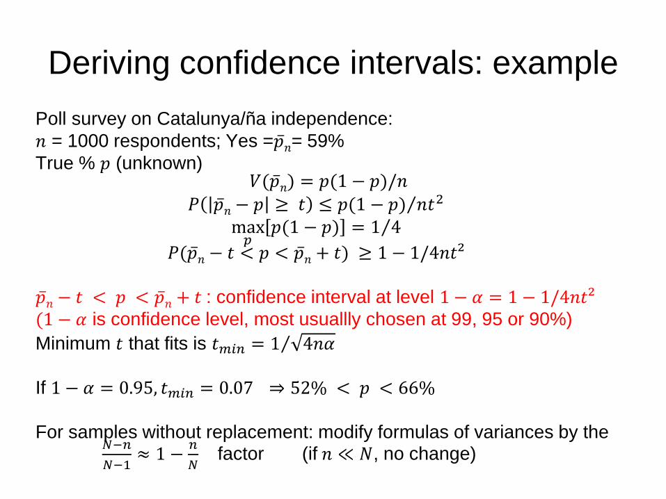
Poll survey on Catalunya/ña independence: 𝑛 = 1000 respondents; Yes =�̅�𝑛= 59% True % 𝑝 (unknown)

𝑉(�̅�𝑛) = 𝑝(1 − 𝑝)/𝑛 𝑃 �̅�𝑛 − 𝑝 ≥ 𝑡 ≤ 𝑝(1 − 𝑝) 𝑛𝑡2⁄

max𝑝

𝑝(1 − 𝑝) = 1 4⁄ 𝑃(�̅�𝑛 − 𝑡 < 𝑝 < �̅�𝑛 + 𝑡) ≥ 1 − 1/4𝑛𝑡𝑅

�̅�𝑛 − 𝑡 < 𝑝 < �̅�𝑛 + 𝑡 : confidence interval at level 1 − 𝛼 = 1 − 1/4𝑛𝑡𝑅 (1 − 𝛼 is confidence level, most usuallly chosen at 99, 95 or 90%) Minimum 𝑡 that fits is 𝑡𝑚𝑖𝑛 = 1 4𝑛𝛼⁄ If 1 − 𝛼 = 0.95, 𝑡𝑚𝑖𝑛 = 0.07 ⇒ 52% < 𝑝 < 66% For samples without replacement: modify formulas of variances by the

𝑁−𝑛𝑁−1

≈ 1 − 𝑛𝑁

factor (if 𝑛 ≪ 𝑁, no change)

Deriving confidence intervals: example

Central Limit Theorem When 𝑛 → +∞:

𝑛 (𝑋�𝑛 − 𝜇) / 𝜎 𝑑→ 𝑁(0,1)

Not only 𝑋�𝑛 gets closer to 𝜇, but its distribution around 𝜇 tends to be normal when 𝑛 is large

σ is usually unknown but law of large numbers also applies to it: For all 𝜀 > 0, lim

𝑛→+∞𝑃( |𝑆𝑛𝑅 − 𝜎2| ≥ 𝜀) = 0

With 𝑆𝑛𝑅 = 1𝑛−1

∑ (𝑋𝑖 − 𝑋�)𝑅𝑛𝑖=1 , such that 𝐸 𝑆𝑛𝑅 = 𝜎2

[ the 1𝑛−1

term stems from the fact that 𝐸 𝑋�𝑛2 = 𝐸 𝑋 𝑅 + 1𝑛𝑉(𝑋)]

Then: 𝑛 (𝑋�𝑛 − 𝜇) /𝑆𝑛𝑑→ 𝑁(0,1)

With small samples of course, normality is not granted (must be assumed for inference)

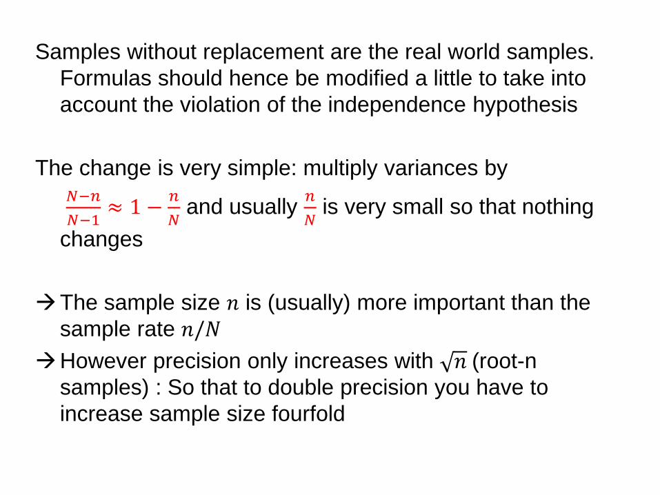
Samples without replacement are the real world samples. Formulas should hence be modified a little to take into account the violation of the independence hypothesis

The change is very simple: multiply variances by

𝑁−𝑛𝑁−1

≈ 1 − 𝑛𝑁

and usually 𝑛𝑁

is very small so that nothing changes

The sample size 𝑛 is (usually) more important than the

sample rate 𝑛/𝑁 However precision only increases with 𝑛 (root-n

samples) : So that to double precision you have to increase sample size fourfold

Two-stage samples 1) draw primary sample units (PSU): 𝑛 units 𝑗 among 𝑁 2) draw secondary units in each PSU: [Sometimes a census of PSUs is implemented to have or to

update PSU size 𝑀𝑗]

𝑚𝑗 units among 𝑀𝑗 (in PSU 𝑗 of size 𝑀𝑗)

(a) fixed number of units 𝑚𝑗 = 𝑚 (b) or fixed sample rate f: 𝑚𝑗 = 𝑓.𝑀𝑗, or full census (f=1) (LFS in France)

Design effects (1) Take home message: clustering is cheaper

economically but costly statistically Except that clustering is also useful for some

analysis Taking into account the survey design

(stratification also, but mostly clustering) is very important for statistical inference

More generally violation of individual errors independence has to be scrutinized everytime

Design effects (2) 𝐷𝐷𝑓𝑓 =

𝑉𝑉𝐶2𝑆(𝑌��)

𝑉𝑉𝐶1𝑆 𝑌��

With replacement to simplify:

𝑉𝑉𝐶1𝑆 𝑌�� = 𝑆2

𝑛𝑚 (Recall: n PSUs, m units in each PSU)

𝑉𝑉𝐶2𝑆 𝑌�� = 1𝑛𝑆1𝑅 + 1

𝑛𝑚 𝑆2𝑅

𝑆1𝑅 = 𝑆𝑅𝜌, variance inter-PSUs ; 𝑆2𝑅 = 𝑆𝑅 (1 − 𝜌) variance intra-PSUs 𝐷𝐷𝑓𝑓 = 1 + (𝑚− 1) 𝜌 More details (without replacement): see e.g. https://dhsprogram.com/pubs/pdf/WP30/WP30.pdf

Unequal probability sampling (1) Example of 2-stage sampling. Based on a population census 1) Draw PSUs 𝑗 𝑛 times with inclusion probability 𝑃𝑗 is proportional to

size 𝑀𝑗 (observed in census)

𝑃𝑗 = 𝑛𝑁

.𝑀𝑗𝑀�

with 𝑀� = 1𝑁∑ 𝑀𝑗𝑁𝑗=1 (mean size)

[ Note: The sum of inclusion probabilities is equal to the sample size n; it is the probability of samples that contain 𝑗 in all size n samples potentially drawn, the total number of which is 𝑁𝑛 = 𝑁!

𝑁−𝑛 !𝑛! ]

2) Prob of inclusion of sec. unit 𝑖 in PSU 𝑗 = Π𝑖𝑗 =? a1) If fixed number of units 𝑚 in each 𝑗: Π𝑖𝑗

= 𝑃𝑗 . (𝑚/𝑀𝑗) = (𝑛.𝑚)/(𝑁.𝑀�) Equal probability

Unequal probability sampling (cont’d)

a2) If updated size 𝑀𝑗* after enumeration is different from ex-ante (census-based) size 𝑀𝑗:

Π𝑖𝑗 = 𝑃𝑗 .

𝑀𝑗

𝑀𝑗∗𝑚𝑀𝑗

= 𝑀𝑗

𝑀𝑗∗ . (𝑛.𝑚)/(𝑁.𝑀�)

b) If fixed sample rate 𝑓 in each PSU: 𝑚𝑗 = 𝑓 .𝑀𝑗 Π𝑖𝑗 = 𝑃𝑗. (𝑚𝑗/𝑀𝑗) = 𝑃𝑗. 𝑓 = (𝑛.𝑚𝑗)/(𝑁.𝑀)

Unequal probability « Sample weights »

Unequal probability sampling (end)

In any case: Estimator of expected value: weighted mean µ𝑦 = Σ𝑗Σ𝑖 𝑦𝑖𝑗 / Π𝑖𝑗

Where sample weight = 1/ Π𝑖𝑗

Check for the existence of sampling weights! Sampling weights sum to one Extrapolation weights sum to total

population

Stratification K strata: for ex., capital city, big cities, etc. or

administrative regions Sample size 𝑛𝑘 in each stratum, heterogeneous

sample rates 𝑓𝑘 = 𝑛𝑘/𝑁𝑘 Unequal prob. 1)Ensures minimal sample sizes in each stratum 2)May be variance reducing if stratum sufficiently

correlated with outcomes measured 3)Usually comes with 2-stage samples, hence

variance reduction from stratification counterbalanced by variance inflation from clustering

Satellites for sampling

A very brief history of stat(e)-istics

• Land property (writing), then cadastre • Fiscal income based on population

(censuses), trade (customs), production (agricultural censuses in Rome)…

• (Control of) Prices & wages (Diocletian edict)

• National accounts (Quesnay) • Probability theory and sample surveys • Internet data, satellite data

Where to get some data on the Web?

More and more data, macro and micro, becomes freely available on the Web. Suggestions will be given within each session.

- UN, IMF, World Bank, WTO, ILO, OECD, Eurostat… + national statistical institutes

- Pop. censuses: IPUMS initiative - Survey series: DHS, LSMS (WB), General

Values Surveys, Rand Corporation surveys…

Some free micro data on the Web IPUMS international (census data): https://international.ipums.org/international/ Demographic and Health Surveys: http://www.measuredhs.com/ World Values Surveys: http://www.worldvaluessurvey.org/ Rand Corporation surveys: http://www.rand.org/labor/FLS/ Some LSMS surveys (World Bank): http://iresearch.worldbank.org/lsms/lsmssurveyFinder.htm African Poverty Databank (World Bank): http://www4.worldbank.org/afr/poverty/databank/cdroms/default.cfm Other free data on WebPages of academics who produced data…

3- Nightlights and GDP (1) Xi Chen, William D. Nordhaus, Using luminosity data as a proxy for economic statistics, Proceedings of the National Academy of Sciences, May 2011, 108 (21) 8589-8594

𝑦 = 𝑦∗ + 𝜀 y = GDP (in log term) 𝑚 = 𝛼 + 𝛽𝑦∗ + 𝑢 m = luminosity (in log as well) Assume we have an estimate for 𝜎𝜀 (see sessions on GDP and prices)

Regression of m on y gives estimate �̂� Corrected 𝛽� = 𝜎𝜀² +𝜎𝑦∗²𝜎𝑦∗²

�̂�

Define: �̂� = 1𝛽�𝑚 And: 𝑥� = 1 − 𝜃 𝑦 + 𝜃�̂� (𝐸 𝑥� = 𝑦∗)

Then:

𝑉 𝑥� = 𝐸 1 − 𝜃 𝑦 + 𝜃�̂� − 𝑦∗ 2 = 𝐸 1 − 𝜃 𝜀 + 𝜃 1𝛽�𝑢

2=(1 − 𝜃)2𝜎𝜀²+ 𝜃2 1

𝛽�2𝜎𝑢²

Optimal: 𝜃∗ = 𝛽�2𝜎𝜀²𝛽�2𝜎𝜀²+𝜎𝑢² Differentiated by type of countries (with different 𝜎𝜀)

Statistical units can be countries or grid-cells (1°× 1°)

3- Nightlights and GDP (2) Xi Chen, William D. Nordhaus, Using luminosity data as a proxy for economic statistics,

Proceedings of the National Academy of Sciences, May 2011, 108 (21) 8589-8594

3- Nightlights and GDP (3) Xi Chen, William D. Nordhaus, Using luminosity data as a proxy for economic statistics,

Proceedings of the National Academy of Sciences, May 2011, 108 (21) 8589-8594

3- Nightlights and GDP (4) All Africa Xi Chen, William D. Nordhaus, Using luminosity data as a proxy for economic statistics,

Proceedings of the National Academy of Sciences, May 2011, 108 (21) 8589-8594