Ocean Modelling 25 (2008) 17–34

Contents lists available at ScienceDirect

Ocean Modelling

journal homepage: www.elsevier .com/ locate/ocemod

Inverse barotropic tidal estimation for regional ocean applications

O.G. Logutov *, P.F.J. LermusiauxMassachusetts Institute of Technology, Department of Mechanical Engineering, 77 Massachusetts Avenue, Room 5-207B, Cambridge, MA 02139, USA

a r t i c l e i n f o

Article history:Received 29 January 2008Received in revised form 21 May 2008Accepted 11 June 2008Available online 25 June 2008

1463-5003/$ - see front matter � 2008 Elsevier Ltd. Adoi:10.1016/j.ocemod.2008.06.004

* Corresponding author. Tel.: +1 617 324 3541; faxE-mail addresses: logutov@mit.edu (O.G.

(P.F.J. Lermusiaux).

a b s t r a c t

Correct representation of tidal processes in regional ocean models is contingent on the accurate specifi-cation of open boundary conditions. This paper describes a new inverse scheme for the assimilation ofobservational data into a depth-integrated spectral shallow water tidal model and the numerical imple-mentation of this scheme into a stand-alone computational system for regional tidal prediction. A novelaspect is a specific implementation of the inverse which does not require an adjoint model. An optimiza-tion is carried out in the open boundary condition space rather than in the observational space or modelstate space. Our approach reflects the specifics of regional tidal modeling applications in which openboundary conditions (OBCs) typically constitute a significant source of uncertainty. Regional tidal modelsrely predominantly on global tidal estimates for open boundary conditions. As the resolution of globaltidal models is insufficient to fully resolve regional topographic and coastal features, the a priori OBC esti-mates potentially contain an error. It is, therefore, desirable to correct these OBCs by finding an inverseOBC estimate that is fitted to the regional observations, in accord with the regional dynamics and respec-tive error estimates. The data assimilation strategy presented in this paper provides a consistent andpractical estimation scheme for littoral ocean science and applications where tidal effects are significant.Illustrations of our methodological and computational results are presented in the area of Dabob Bay andHood Canal, WA, which is a region connected to the open Pacific ocean through a series of inlandwaterways and complex shorelines and bathymetry.

� 2008 Elsevier Ltd. All rights reserved.

1. Introduction

Coastal dynamical phenomena can be significantly affected bytidal processes. Tidal currents constitute a dominant componentof circulation in many coastal areas, with velocities of 50–150 cm/s being common (e.g., Moody et al., 1984). Tidally drivencurrents may generate complex cross-shelf particle transports,highly horizontally inhomogeneous barotropic flow patterns, aswell as important secondary tidally-driven features, such as inter-nal tides, internal waves, tidal mixing and tidal fronts (Chen andBeardsley, 1998). Tidal processes are also important for ocean eco-system dynamics on a regional scale. For example, distinct patternsof nutrient patchiness, have been observed in some tidally activebasins; arguably controlled by tidal processes (e.g., Franks andChen, 1996). Correct representation of these tidal processes in re-gional ocean models is paramount but challenging.

Accurate barotropic tidal estimates (tidal elevations, transports,and velocities) are needed in numerous oceanographic applica-tions. These include physical modeling and acoustical, chemical,biological, and eco-system modeling applications. For example,the determination of the internal tides requires an accurate knowl-edge of barotropic transports and flows across bottom topography

ll rights reserved.

: +1 617 324 3541.Logutov), pierrel@mit.edu

as such flows are utilized as forcing in internal tide models (Baines,1982; Garrett and Gerkema, 2007). These internal tide models, intheir turn, are needed in acoustical (Lermusiaux and Chiu, 2002)and biological applications (e.g., Besiktepe et al., 2003) becausethe vertical velocity field and the temperature and density pertur-bations induced by internal tides and wave are consequential inthese applications. The ‘‘state-of-the-art” for modeling tidal phe-nomena in regional ocean applications is currently based on forc-ing primitive equation (PE) or non-hydrostatic ocean modelswith barotropic tidal fields. This tidal forcing is applied throughopen boundary and initial flow conditions. If the horizontal andvertical model resolutions are sufficient and accurate regionalbarotropic tidal forcing is used, this approach can simulate a largespectrum of tidally driven processes. For example, effects of inter-nal tides and waves can be generated and represented statisticallyand possibly deterministically in limited regions.

Regional tidal models rely on global tidal models (Shum et al.,1997), larger scale models, and/or extrapolation from local tidegauges for open boundary conditions (OBCs). For example, thetwo Navy tidal modeling systems, ADCIRC (Luettich et al., 1992)and PCtides (Hubbert et al., 2001), use the tidal harmonic constit-uents extracted from the global FES95 solutions (LeProvost et al.,1994), as well as extrapolation from local tide gauges (Blain etal., 2002). Greenberg et al. (2005) obtain the OBCs for the Quoddyregion of the Bay of Fundy from an outer Bay of Fundy regional

18 O.G. Logutov, P.F.J. Lermusiaux / Ocean Modelling 25 (2008) 17–34

model. Foreman and Thomson (1997) use the elevation amplitudesand phases at the southern and western boundaries around thecoast of Vancouver Island from a combination of offshore pressuretide gauges and the global tidal model of Egbert et al. (1994). Cor-rect representation of tidal processes on a regional scale is contin-gent on the accurate specification of OBCs. Errors in OBCs cangenerate physically unrealistic flow fields and lead to large interiordata-model misfits. It is, therefore, desirable to tune the OBCs to lo-cal observations.

The need for dynamical constraints to optimally extrapolatereliable sea level data on the coastline to tidal model open bound-aries has long been recognized (Bennett and McIntosh, 1982). Avariety of methods have been developed to constrain regionalbarotropic tidal estimates using tidal elevation and velocity obser-vations (see Section 2). Despite of wide recognition that a quanti-tative fit of the OBCs to local observational data is highlydesirable, it is often omitted or carried out by simple trial and errorthrough the comparison of model outputs with tidal elevationamplitudes and phases at local tide gauge stations (e.g., Foremanand Thomson, 1997; Greenberg et al., 2005) among others. Thisimplicitly attests to the fact that new methods to fit OBCs to data,that are practical and amenable to quick implementation, are stillneeded. The data assimilation strategy presented in this paper isdesigned specifically to provide a highly practical and quantitativetechnique for the fit of OBCs to tidal data in regional tidal modelingapplications.

This paper describes new forward and inverse schemes for esti-mating regional barotropic tidal flows and the numerical imple-mentation of these schemes into a stand-alone computationalsystem. The data-driven prognostic schemes are based on solvingthe depth-integrated shallow water equations as a boundary valueproblem in the spectral domain. With our system, regional baro-tropic tides can be computed at very high resolution in multiplenested domains. The observational data are assimilated into the ti-dal model through a practical inverse method. The outputs of thesystem are accurate high-resolution barotropic tidal fields thatcan be utilized to force the open boundary of any modern regionalPE or non-hydrostatic ocean model. Synthesis of observations andnumerical models has long been recognized as a necessary steptowards successful coastal prediction (Robinson et al., 1998;Lermusiaux, 2006). With our new procedures, the measurementsare assimilated in such a way that the inverse tidal estimatessatisfy the shallow water equations exactly.

Our barotropic tidal estimation system can be used for specifictidal studies and for forcing PE and internal wave models. Pres-ently, it is illustrated with the Harvard Ocean Prediction System(HOPS), an interdisciplinary primitive equation modeling systemdesigned primarily for regional ocean applications with advanceddata assimilation (DA) (Robinson, 1999; Lermusiaux, 1999). Thefree-surface version of HOPS requires barotropic tidal forcings (ti-dal sea surface height and barotropic velocity components) at openboundaries and for initialization. These barotropic tidal forcingsare obtained using the new forward–inverse system described inthis paper. Because the barotropic tidal model is designed to sim-ulate a specific process and serve a specific range of spatial-tempo-ral scales, we are able to simulate the barotropic tides at very highresolution and tune its OBCs and model parameters to available re-gional tide gauges and Acoustic Doppler Current Profiler (ADCP)data. This new methodology is an example of a multi-model ap-proach, with several specialized models combined together in asingle ocean prediction system. More general discussion of uncer-tainties and implementation of multi-model simulations are pro-vided in Logutov and Robinson (2005), Logutov (2007),Evangelinos et al. (2006), Lermusiaux et al., 2004.

We have exercised our tidal modeling approach in multipleregional applications. These include real-time modeling in the

Middle Atlantic Bight and the shelf-break front region off the coastof New Jersey, as part of the Autonomous Wide Aperture Clusterfor Surveillance (AWACS-06) and Shallow Water (SW06) experi-ments, in the California Current System and Monterey Bay regionas part of the Monterey Bay-06 (MB06) experiment which followedour work during AOSN-II (Haley et al., in press; Lermusiaux, 2007)in that region, and in the Hood Canal and Dabob Bay region, WA, aspart of the PLUSNet-07 (PN07) experiment (Xu et al., 2008). Our ti-dal modeling work in the Hood Canal and Dabob Bay, particularlychallenging given the complexity of shoreline and bottom topogra-phy of the inland waterways connecting this basin to the ocean, isselected here to exemplify our approach and method.

The paper is organized as follows. Existing regional tidal modelsand assimilation schemes pertinent to the new techniques de-scribed in this paper are briefly reviewed next (Section 2). In Sec-tion 3, the dynamical equations for linearized barotropic shallowwater dynamics and the corresponding boundary value problemin the spectral domain are outlined. Section 4 covers the numericalsolution of the dynamical equations, with details of the numericalimplementation provided in Appendix B. Section 5 describes theproposed method of inverse estimation of OBCs designed for regio-nal tidal modeling. Discussion of our method and its comparison tothe representer method, an approach for DA utilized in global tidalmodeling (Egbert et al., 1994; Egbert and Erofeeva, 2002), are givenin Section 6. Finally, Section 7 presents an illustration of a real-world tidal modeling application within the framework of the Per-sistent Littoral Undersea Surveillance Network (PLUSNet) projectin the Dabob Bay/Hood Canal region of WA. Appendices A throughD detail the notation, the specifics of our numerical implementa-tion, and of the conversion of data from time to model spectral do-main and back, respectively.

2. A synopsis of tidal modeling and data assimilation

A variety of methods for barotropic tidal modeling has beendeveloped and analyzed in the literature. Differences among thesemethods are in the formulation of the horizontal coordinates, inthe inclusion or omission of the vertical structure of tidal velocityfields, and in the treatment of the time dependency and of thenon-linear terms. The horizontal coordinate formulations includefinite-difference schemes (e.g., Davies, 1993; Hubbert et al.,2001), finite-element schemes (e.g., LeProvost and Vincent, 1986;Luettich et al., 1992; Greenberg et al., 2005; Bernard et al., 2008),and structured non-orthogonal curvilinear coordinate schemes(e.g., George, 2007). Two-dimensional (e.g., McLaughlin et al.,2003) and three-dimensional (e.g., Jones and Davies, 1996; Davieset al., 1997c) barotropic tidal models have been proposed to allowfor omission or inclusion of the computation of bottom and surfaceboundary layers as well as of the vertical current structure,especially effects of turbulent fluxes and their parameterizations(e.g., Davies, 1993; Davies and Gerritsen, 1994; Davies et al.,1997b; Foreman and Thomson, 1997; Lee and Jung, 1999). Themodels differ by their treatment of the time dependency and fallinto classes of time-domain (e.g., Le Cann, 1990; Lynch and Gray,1979) and spectral-domain (e.g., LeProvost et al., 1981; Lynchand Naimie, 1993; Davies et al., 1997a) models.

Two alternative treatments of the time dependency, by timestepping (e.g., Lynch and Gray, 1979) and by spectral representa-tion (e.g., LeProvost et al., 1981), have been exercised. The spectraldomain representation assumes harmonic time dependency foreach tidal constituent and leads to a substantial reduction of modelcomputational complexity and, therefore, potentially to higher res-olution models. The coupling between different tidal frequenciesthat arises from the nonlinear interactions can be included in thespectral domain models using a perturbation method (Snyder et

O.G. Logutov, P.F.J. Lermusiaux / Ocean Modelling 25 (2008) 17–34 19

al., 1979). A review of spectral domain tidal models in regionalocean applications is provided by Davies et al. (1997a). In additionto substantial computational efficiency, spectral domain modelsare easier in use and, as such, more suitable for disseminationamong a wider audience of researchers. The time stepping models,on the other hand, are more amenable to inclusion of the nonlinearterms and more suitable for modeling ocean response to a generaltime-dependent meteorological forcing (e.g., Luettich et al., 1992).

The relative importance of the various nonlinear mechanisms forregional barotropic tidal modeling is reviewed by Parker (1991).Theoretically, nonlinear processes act as an agent for energy transferto higher harmonics and are capable of introducing new frequenciesin tidal spectrum. A number of fully nonlinear regional tidal modelshave been developed (Le Cann, 1990, among others; Luettich et al.,1992; George, 2007). The nonlinear tidal effects can also be simu-lated by using the primitive equation or non-hydrostatic modelswith the open boundary tidal forcing prescribed from the tidal mod-els. If open ocean boundaries of a PE model are selected away fromthe shallow-water regions, significant gains in accuracy can resultfrom using linearized high-resolution data-assimilative barotropictidal models, rather than their non-linear counterparts, to prescribethe tidal open boundary forcing for PE models.

A number of methods have been developed to include the non-linear tidal effects within the linearized modeling framework. Forexample, the shallow-water tidal constituents can be introducedto compensate for kinematic and dissipative nonlinearities andfor wave–wave interactions between the astronomical constitu-ents (LeProvost et al., 1981; Andersen et al., 2006). The character-istics of the shallow-water constituents can either be empiricallydetermined from the observational data (e.g., Hea et al., 2004;Simpson, 1998) or obtained analytically using a classical perturba-tion method (LeProvost et al., 1981). In the latter case, the fullynonlinear problem can be reduced to a sequence of linearizedboundary value problems, similar to the boundary value problemdescribed in Section 3, for each successive order of approximationof the perturbation method (e.g., LeProvost and Vincent, 1986). Inpractice, the perturbation sequence is typically limited to the sec-ond order. These developments provide a rigorous framework forfull inclusion of the nonlinear effects into robust high-resolutionlinearized data-assimilative computations.

Importantly, all regional tidal modeling systems require specifi-cation of the open boundary conditions (OBCs). The early coastaltidal DA and parameter estimation work is reviewed in Sections5.1–2 of Robinson et al. (1998). Bennett and McIntosh (1982)developed a variational formulation to consistently constrain re-gional tidal estimates with local observations. The formulation isin the time domain. It solves the equations of the first variationof the quadratic cost function penalizing model-data misfits aswell as deviations of the generalized inverse solution from the for-ward model solution, weighted by observational and model errorcovariance estimates. This generalized inverse methodology wasfurther applied for modeling M2 tides in Bass Strait north ofTasmania (McIntosh and Bennett, 1984) and has become a founda-tion for a variety of representer methods for tidal data inversion,interpolation, and inference (Egbert, 1997). For instance, Egbertet al. (1994) assimilate TOPEX/POSEIDON altimeter data and tidegauge data into global barotropic tidal models. The method re-quires formulation of an adjoint tidal model. An optimization iscarried out in the observational space by generalized inversion(Bennett, 1992; Bennett, 2002). Reduced-basis alternatives of therepresenter method have latter been applied for tidal DA (Egbertand Erofeeva, 2002). Representer-based inverse models have alsobeen formulated for estimation of the internal tides (Kurapovet al., 2003), as well as other coastal ocean modeling problems(Kurapov et al., 2007). Hybrid schemes have also been developed.For example, He and Wilkin (2006) have successfully utilized a full

primitive equation model with uniform density to obtain the non-linear forward tidal solution. Subsequently, a linear, frequency-do-main, finite-element model is employed for the inverse problem,assimilating tidal observations by minimizing a least-squaredata-model misfit criterion. Zou et al. (1995) also developed asequential open-boundary control scheme augmenting radiationconditions and applied it to idealized barotropic wind-drivenocean simulations.

Kalman Filtering (KF) and other sequential DA techniques havebeen extensively applied in the context of deterministic and sto-chastic hydrodynamic, water quality, and surface wave regionalforecasting and hind-casting and for error covariance modeling(e.g., see Section 5 in Robinson et al., 1998). For example, theKF approach has recently been adopted as an operational methodfor assimilation of sea-level measurements into the DutchContinental Shelf model utilized at the Dutch MeteorologicalInstitute to predict water levels along the Dutch coast and thethree-dimensional flow fields in the North and the Baltic seabasins (Sorensen and Madsen, 2004). Other examples includeoperational shelf sea modeling in Danish waters carried out atthe Danish Meteorological Institute (Canizares et al., 2001). Kal-man filter algorithms rely on propagating an uncertainty in themodel state-space using linearized error covariance evolutionequations or Monte–Carlo techniques. The error covariance evolu-tion is formulated in the state-space form, with gridded waterlevels, velocities, and the uncertain parameters included in a statevector. Low-rank and ensemble approximations have been de-scribed and applied in realistic settings, and various regulariza-tion techniques for error covariance and Kalman gain estimationhave been introduced, including temporal smoothing, the stea-dy-state approximation, and spatial regularization, among others(Sorensen and Madsen, 2004). An efficient KF data assimilationprocedure for weakly nonlinear regional tidal models has beenformulated by Heemink and Kloosterhuis (1990). The dynamicalequations were embedded into a stochastic environment andthe state-space was evolved using the non-linear stochastic shal-low water equations to obtain a constant-gain extended-KFapproximation. The steady-state KF method is founded on anobservation that error covariances often tend to a quasi-steadystate after a few days of assimilation. Therefore, a time invariantKalman gain could be obtained off-line and applied without theneed to be recomputed as new measurements became available.The method was originally applied for assimilation of water levelmeasurements into a tidal model of the North Sea and, subse-quently, in numerous other applications in simulated and realisticsettings (Canizares et al., 2001; Sorensen and Madsen, 2004). Amain difficulty of the KF-based algorithms is related to thequantification of the stochastic noise processes or model errorcovariance parameters employed in the scheme (Dee, 1995;Lermusiaux, 2006; Lermusiaux et al., 2006). Other DA practicesin regional tidal modeling include use of weighted nudging toloosely constrain model tidal heights to observed sea-level eleva-tions at available tidal stations (e.g., Navy PCTides system ofHubbert et al., 2001). Das and Lardner (1992) use water depthand bottom friction coefficients as tunable parameters in adepth-averaged linearized tidal model in the time domain. Theyemploy an adjoint scheme to solve the optimization problem offitting the tunable parameters to observations.

The new regional DA scheme developed in this paper differsfrom the previous schemes mostly in two ways. Firstly, an optimi-zation is carried out in the open boundary condition space ratherthan in the observational space or full state space. Our strategyof using the OBCs as the control space for data assimilation reflectsthe specifics of regional tidal modeling. Secondly, our approachdoes not require an adjoint model. The specifics of the implemen-tation are such that only the forward dynamical model is needed.

20 O.G. Logutov, P.F.J. Lermusiaux / Ocean Modelling 25 (2008) 17–34

Of course, variations of our approach and hybrid schemes arepossible. They are outlined in the conclusions.

3. Dynamical equations

Regional and global tidal flow fields are predominantly con-trolled by different types of tide-generating forcing. In global tidalmodels, the forcing is provided by direct astronomical gravitationalforces prescribed through a tide-generating potential. In regionalapplications, tidal forcing is primarily provided through the openboundary conditions. In shallow water, direct astronomical forcingis negligible as compared to open boundary forcing and can beomitted from the hydrodynamic equations (Snyder et al., 1979;Simpson, 1998). Similarly, tidal loading effects related to the defor-mation of the earth crust under the load of a tidal wave, importantfor global tidal modeling, are negligible in regional applications. Inthe present paper, we are concerned exclusively with shallow searegions and, therefore, the tide generating forces and tidal loadingcorrections can be omitted from the hydrodynamic equations.

3.1. Time domain

Given a regional basin X, with open boundary segments oXO

and closed boundary segments oXC , the linearized barotropic shal-low water equations are derived from vertical integration over thewater column of the three-dimensional momentum and continuityequations subject to the hydrostatic and Boussinesq approxima-tions (Lynch and Gray, 1979). Using spherical coordinates in thehorizontal, we obtain

o

otgþ 1

a cos /o

okðHuÞ þ 1

a cos /o

o/ðHv cos /Þ ¼ 0

o

otu� fvþ Fk ¼

�ga cos /

o

okg

o

otvþ fuþ F/ ¼

�ga

o

o/g

ð1Þ

for ðk;/Þ 2 X, subject to open boundary conditions

gjoXO¼ gobc ð2Þ

and closed boundary conditions

n � ujoXC¼ 0: ð3Þ

In the foregoing, g and u ¼ ðu; vÞ denote tidal elevation and zonaland meridional velocity components, k, /, and a are the longitude,latitude, and earth radius, H, g, and f denote the undisturbed waterdepth, acceleration due to gravity, and the Coriolis parameter, andFk and F/ are the parameterized friction forces in the zonal and themeridional directions, respectively. Inherent in Eq. (1) is omissionof the non-linear advective terms ðu � $Þu. We will further requirethat the dissipative terms Fk and F/ are also linearized in some fash-ion. The linearization is introduced in order to make the governingequations amenable to reduction to a linear system of algebraicequations once they are discretized on a selected grid. As mentionedin Section 1, linearized models have an important role and multipleapplications. Quadratic friction of the form

Fk ¼ CDjuju=H; F/ ¼ CDjujv=H ð4Þ

with non-dimensional bottom drag coefficient CD ¼ 0:002� 0:003is typically suggested for depth-averaged barotropic tidal models(Grenier et al., 1995). Linearization of quadratic dissipation termsFk � jðk;/Þu; F/ � jðk;/Þv, with a spatially varying damping coef-ficient jðk;/Þ, can be obtained for example using the perturbationmethod developed by LeProvost et al. (1981). Alternatively, aniterative approach can be applied in which the 0th iteration ofthe solution is obtained with a constant value of j, while the next

iteration solution utilizes the barotropic velocities obtained in theprevious iteration for juj in (4). We follow the latter approach,with one iteration. A detailed review of bottom friction parameter-izations suitable for barotropic ocean tidal models is beyond thescope of this paper but has been addressed in a number of papers(Grenier et al., 1995; Xing and Davies, 1996; Davies et al., 1997b;Lee and Jung, 1999). With Eq. (1), the linearized barotropic tidalestimates can be obtained and tuned to local observations of baro-tropic tides. Nonlinear tidal effects can then be simulated, ifneeded, by the PE models forced by these linearized barotropictides at open-boundaries. Such approach is acceptable if tidalvelocities are small enough at the offshore open-boundary of aPE model. With these considerations in mind, our focus here isthe linearized inverse barotropic tidal estimation and data assim-ilation in regional applications.

System (1) is forced through open boundary conditionsgobc . In re-gional applications, the open boundary conditions are often speci-fied from global tidal models (Shum et al., 1997). Global tidalmodels typically compute estimates for individual astronomical ti-dal constituents. Astronomical tidal constituent frequencies corre-spond to combinations of fundamental astronomical frequenciesarising from planetary motions (e.g., Simpson, 1998). Each astro-nomical constituent is defined by a unique set of Doodson numberswhich determine its frequency. We specify the open boundary con-dition (2) from a global tidal model as a superposition of K tidal con-stituents estimated to be significant for the given coastal region ofinterest:

gobc ¼ RXK

k¼1

fkðxO; yOÞ exp ixkt

( ); ð5Þ

where R denotes the real parts. Complex fkðxO; yOÞ specifies spatialvariations of boundary forcing in amplitude and phase for the kthtidal constituent along open boundary segments, ðxO; yOÞ 2 oXO. Inour own practice, we utilize global tidal fields of TPXO 7.0 fromOSU (Egbert et al., 1994) for fkðxO; yOÞ in forward computations inthe outer domain and the outer domain solution in the nested do-mains. We select the K significant tidal constituents in Eq. (5) byanalysis of tidal gauges and other current data in the given coastalregion of interest.

Several OBCs other than (5) can be implemented with ourscheme, as discussed in Tsynkov (1998), Marchesiello et al.(2001), Oddo and Pinardi (2008), Blayo and Debreu (2005). Theyinclude radiation-based and characteristic boundary conditions(e.g., Orlanski, 1976; Flather, 1976; Chapman, 1985; Shulman etal., 2002) as well as relaxation conditions and absorbing (sponge)layers (e.g., Davies, 1976; Marchesiello et al., 2001; Lavelle andThacker, 2008). These OBCs for the barotropic tidal model shouldbe consistent with the OBCs used in the primitive equation model(forced by tides) and should account for the different scales andresolutions. The OBCs used in HOPS, including radiation, relaxa-tion, simplified physics and advection-based conditions are re-viewed in Lermusiaux (1997).

In anticipation of reduction of the governing equations to a lin-ear system of algebraic equations for the discretized model state-space, we introduce the matrix notation and express (1) as

o

otgþ $ �

Hu

Hv

� �¼ 0 ð6Þ

oot þ j �f

f oot þ j

" #u

v

� �¼ �g$g ð7Þ

where $� and $ are the divergence and gradient operators in spher-ical coordinates. Eqs. (6) and (7) are solved in the spectral domainin terms of the prognostic variable g. The velocity field is subse-quently obtained from g via (7). The details of the solution nowfollow.

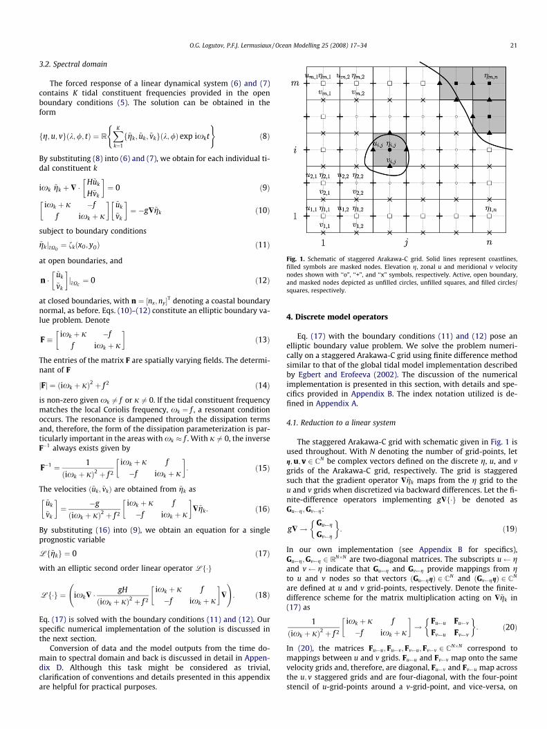
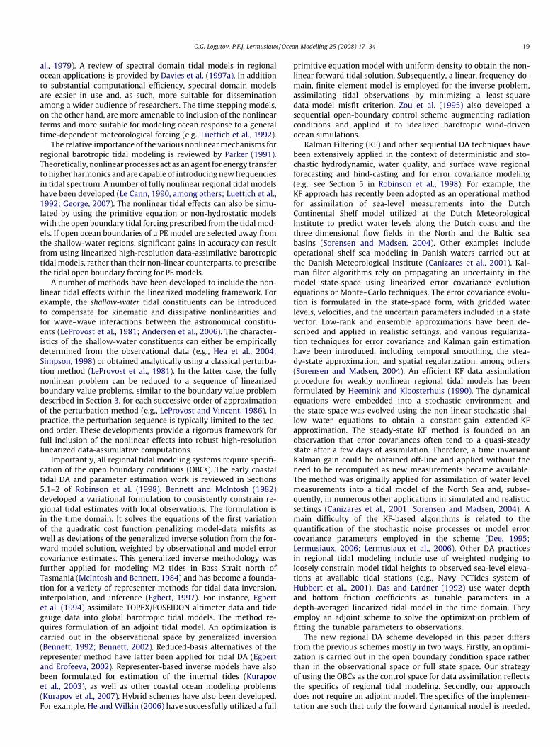
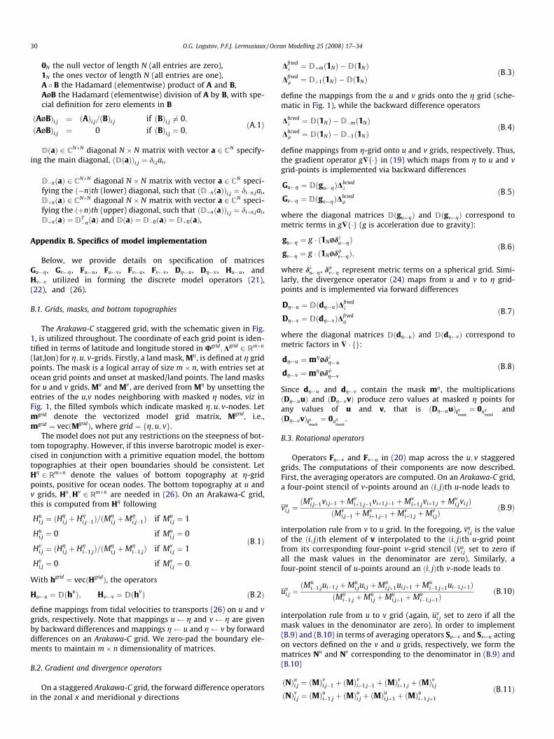
Fig. 1. Schematic of staggered Arakawa-C grid. Solid lines represent coastlines,filled symbols are masked nodes. Elevation g, zonal u and meridional v velocitynodes shown with ‘‘o”, ‘‘+”, and ‘‘x” symbols, respectively. Active, open boundary,and masked nodes depicted as unfilled circles, unfilled squares, and filled circles/squares, respectively.

O.G. Logutov, P.F.J. Lermusiaux / Ocean Modelling 25 (2008) 17–34 21

3.2. Spectral domain

The forced response of a linear dynamical system (6) and (7)contains K tidal constituent frequencies provided in the openboundary conditions (5). The solution can be obtained in theform

fg;u; vgðk;/; tÞ ¼ RXK

k¼1

f~gk; ~uk; ~vkgðk;/Þ exp ixkt

( )ð8Þ

By substituting (8) into (6) and (7), we obtain for each individual ti-dal constituent k

ixk ~gk þ $ �H~uk

H~vk

� �¼ 0 ð9Þ

ixk þ j �f

f ixk þ j

� �~uk

~vk

� �¼ �g$~gk ð10Þ

subject to boundary conditions

~gkjoXO¼ fkðxO; yOÞ ð11Þ

at open boundaries, and

n �~uk

~vk

� �joXC¼ 0 ð12Þ

at closed boundaries, with n ¼ ½nx;ny�T denoting a coastal boundarynormal, as before. Eqs. (10)–(12) constitute an elliptic boundary va-lue problem. Denote

F �ixk þ j �f

f ixk þ j

� �ð13Þ

The entries of the matrix F are spatially varying fields. The determi-nant of F

jFj ¼ ðixk þ jÞ2 þ f 2 ð14Þ

is non-zero given xk 6¼ f or j 6¼ 0. If the tidal constituent frequencymatches the local Coriolis frequency, xk ¼ f , a resonant conditionoccurs. The resonance is dampened through the dissipation termsand, therefore, the form of the dissipation parameterization is par-ticularly important in the areas with xk � f . With j 6¼ 0, the inverseF�1 always exists given by

F�1 ¼ 1

ðixk þ jÞ2 þ f 2

ixk þ j f

�f ixk þ j

� �: ð15Þ

The velocities ð~uk; ~vkÞ are obtained from ~gk as

~uk

~vk

� �¼ �g

ðixk þ jÞ2 þ f 2

ixk þ j f

�f ixk þ j

� �$~gk: ð16Þ

By substituting (16) into (9), we obtain an equation for a singleprognostic variable

Lf~gkg ¼ 0 ð17Þ

with an elliptic second order linear operator Lf�g

Lf�g ¼ ixk$ �gH

ðixk þ jÞ2 þ f 2

ixk þ j f

�f ixk þ j

� �$

!: ð18Þ

Eq. (17) is solved with the boundary conditions (11) and (12). Ourspecific numerical implementation of the solution is discussed inthe next section.

Conversion of data and the model outputs from the time do-main to spectral domain and back is discussed in detail in Appen-dix D. Although this task might be considered as trivial,clarification of conventions and details presented in this appendixare helpful for practical purposes.

4. Discrete model operators

Eq. (17) with the boundary conditions (11) and (12) pose anelliptic boundary value problem. We solve the problem numeri-cally on a staggered Arakawa-C grid using finite difference methodsimilar to that of the global tidal model implementation describedby Egbert and Erofeeva (2002). The discussion of the numericalimplementation is presented in this section, with details and spe-cifics provided in Appendix B. The index notation utilized is de-fined in Appendix A.

4.1. Reduction to a linear system

The staggered Arakawa-C grid with schematic given in Fig. 1 isused throughout. With N denoting the number of grid-points, letg;u; v 2 CN be complex vectors defined on the discrete g, u, and vgrids of the Arakawa-C grid, respectively. The grid is staggeredsuch that the gradient operator $~gk maps from the g grid to theu and v grids when discretized via backward differences. Let the fi-nite-difference operators implementing g$f�g be denoted asGu g;Gv g:

g$!Gu g

Gv g

� �: ð19Þ

In our own implementation (see Appendix B for specifics),Gu g;Gv g 2 RN�N are two-diagonal matrices. The subscripts u gand v g indicate that Gu g and Gv g provide mappings from gto u and v nodes so that vectors ðGu ggÞ 2 CN and ðGv ggÞ 2 CN

are defined at u and v grid-points, respectively. Denote the finite-difference scheme for the matrix multiplication acting on $~gk in(17) as

1

ðixk þ jÞ2 þ f 2

ixk þ j f

�f ixk þ j

� �!

Fu u Fu v

Fv u Fv v

� �: ð20Þ

In (20), the matrices Fu u;Fu v;Fv u; Fv v 2 CN�N correspond tomappings between u and v grids. Fu u and Fv v map onto the samevelocity grids and, therefore, are diagonal, Fu v and Fv u map acrossthe u; v staggered grids and are four-diagonal, with the four-pointstencil of u-grid-points around a v-grid-point, and vice-versa, on

22 O.G. Logutov, P.F.J. Lermusiaux / Ocean Modelling 25 (2008) 17–34

an Arakawa-C grid. The velocity vectors u and v corresponding toð~uk; ~vkÞ in (16) are, thus, obtained via linear operators

Uu g ¼ �Fu uGu g � Fu vGv g ð21ÞVv g ¼ �Fv vGv g � Fv uGu g ð22Þ

acting on the tidal elevation vector g

u ¼ Uu gg

v ¼ Vv gg:ð23Þ

The divergence operator maps from u and v to g grid-points and isimplemented via forward differences on an Arakawa-C grid

$� ! Dg u;Dg v� �

; ð24Þ

where forward difference matrices Dg u;Dg v 2 RN�N (specifics inAppendix B) are two-diagonal. With Hu u and Hv v denoting themappings from velocities to transports (multiplication by H) at uand v grid points, the discretized second order operator (18) is ex-pressed as

Lf�g ! Ag g; ð25Þ

where the matrix Ag g 2 CN�N is given by

Ag g ¼ Dg uHu uUu g þ Dg vHv vVv g þ ixkI: ð26Þ

As described in Appendix B, the matrix Ag g 2 CN�N is nine-diago-nal. Dynamics (17) is thus reduced to

Ag gg ¼ 0: ð27Þ

The vector g 2 CN in the foregoing contains both active, masked andboundary g-grid points. Next, we discuss the solution of (27) for themodel state-space.

4.2. Solution for model state-space

Let iobc denote the index of open boundary nodes, iobc 2 Nnobc

(Appendix A). The sea surface elevation is prescribed accordingto (2) at iobc grid points. We follow the index notation in AppendixA to write the discrete version of the open boundary condition (11)as

ðgÞiobc¼ gobc; ð28Þ

where gobc 2 Cnobc are given values at open boundaries, for exampleprescribed from a global tidal model. Let imask denote the index ofmasked g-points, imask 2 Nnmask . The remaining g-grid points, neitherin imask 2 Nnmask nor in iobc , are the active nodes, with index ix 2 Nnx ,nx ¼ ðN � nobc � nmaskÞ. The entire vector g is, thus, partitioned intothree subsets corresponding to active, open boundary, and maskedgrid points, with indices ig ¼ fix; iobc; imaskg, where ig 2 NN . The val-ues of gk at ix are the unknowns, the values at iobc prescribe the openboundary forcing, while the values at imask are masked and not com-puted. The values gk at active nodes ix are grouped into a modelstate-space vector x 2 Cnx defined as

x ¼ ðgÞixð29Þ

Let also Aðx xÞ and Aðx gobc Þ denote the partitions of matrix Ag g cor-responding to mappings x x and x gobc

Aðx xÞ � ðAg gÞix ;ix; Aðx gobcÞ � ðAg gÞix ;iobc

: ð30Þ

Similarly, denote the partitions of matrices Uu g and Vv g in (21)and (22) corresponding to mappings u x and v x as

Uðu xÞ � ðUu gÞix ;ix; Vðv xÞ � ðVv gÞix ;ix

: ð31Þ

With this notation, the linear system (27) expressed for the un-known state-space x is

Aðx xÞx ¼ �Aðx gobcÞgobc ð32Þ

The linear system (32) is our computational discretization of thedynamical Eq. (17) at active grid-points given the open boundaryconditions gobc . Note, by construction, it avoids any computationsfor masked grid points. The right-hand side of (32) represents oceanopen boundary forcing. In our implementation, (32) is solved usinga preconditioned conjugate gradient method for sparse systems(Trefethen and Bau, 1997). Since an elliptic boundary value problem(17) with BCs (11) and (12) has a unique solution, a properly formedmatrix Aðx xÞ is guaranteed to be full-rank. The rate of convergenceof conjugate gradient solvers degrades as the condition number of amatrix increases. We use an incomplete LU decomposition to obtainthe left and right pre-conditioners for Aðx xÞ before applying of theconjugate gradient method.

Although the inverse matrix A�1ðx xÞ is never formed explic-

itly but rather the linear system Aðx xÞx ¼ b with b ¼�Aðx gobcÞgobc is solved iteratively, we can formally write thesolution of (32) and, using (23), the solution for tidal veloci-ties u and v:

x ¼Mðx gobc Þgobc

u ¼Mðu gobcÞgobc

v ¼Mðv gobcÞgobc

ð33Þ

where

Mðx gobcÞ ¼ �A�1ðx xÞAðx gobcÞ

Mðu gobcÞ ¼ Uðu xÞMðx gobcÞ

Mðv gobcÞ ¼ Vðv xÞMðx gobcÞ

ð34Þ

The system (33) and (34) constitutes the discretized forwarddynamical model, with forcing provided in open boundary condi-tions gobc .

5. Inverse estimation of open boundary conditions

5.1. Observational data and observational models

Suppose some observational data of tidal elevation and/orvelocity are available in the model domain. Typically, tidal obser-vations are collected along coasts and in inland waterways,although some measurements can come from moorings, ADCPs,and bottom mounted tide gauges. Care should be exercised inensuring that the model resolution is sufficient to resolve the topo-graphic features and waterways around the tide gauges utilized sothat the measurements chosen for assimilation are representativeof the model tidal fields. Let vectors gobs 2 Cng

obs , uobs 2 Cnuobs , and

vobs 2 Cnvobs contain the observed values of barotropic tidal eleva-

tions gk, and barotropic zonal and meridional tidal velocity compo-nents uk,vk at selected observational locations. Let also Hgobs x,Huobs u, and Hvobs v denote the linear observational operators relat-ing the state-space x and the gridded values of velocities u and v tothe observed values gobs, uobs and vobs, respectively. If the observa-tions gobs, uobs and vobs are converted to harmonic amplitudes forbarotropic tidal constituents (Appendix D) then the operatorsHgobs x, Huobs u, Hvobs v merely represent the interpolation fromthe model grid to the observation locations. With the above nota-tion, the data-model misfits in tidal elevation and velocity fieldsare given by

dg ¼ gobs �Hgobs xx;du ¼ uobs �Huobs uu;dv ¼ vobs �Hvobs vv;

ð35Þ

where ðx, u, vÞ are model state-space and model velocity vectors.Lets arrange dg, du, and dv into a single data-model misfit vectord 2 Cnobs of length nobs ¼ ðng

obs þ nuobs þ nv

obsÞ

O.G. Logutov, P.F.J. Lermusiaux / Ocean Modelling 25 (2008) 17–34 23

d ¼dx

du

dv

264

375

nobs

ð36Þ

and use y 2 Cnobs to denote the full observational vector

y ¼gobs

uobs

vobs

264

375

nobs

: ð37Þ

Taking into account (23) with partitions (31), the observationaloperator projecting the state-space x onto the observational spacecorresponding to y is then given by

H ¼Hgobs x

Huobs uUu x

Hvobs vVv x

264

375

nobs�nx

ð38Þ

and the data-model misfits are obtained as

d ¼ y �Hx: ð39Þ

5.2. Observational and OBC error covariances

Let g, u, v denote the true values of tidal elevation and veloc-ities on their respective staggered model grids, while g, u, v de-note the corresponding estimates. The true values of the griddedopen boundary conditions gobc 2 Cnobc are related to the estimategobc as

gobc ¼ gobc þ �obc ð40Þ

where �obc is the unknown OBC error. Let Bobc denote the openboundary condition error covariance

Bobc � Ef�obc�Hobcg: ð41Þ

In practice, Bobc is not well known (e.g., Egbert et al., 1994). It can bespecified via a parametric form with some assumed OBC error param-eters reflecting the accuracy information provided with the OBC val-ues or estimated by the regional modeler. Choosing the OBC errorcovariance parameters amounts to specifying a statistical upper limitfor the OBC correction that a modeler deems appropriate to intro-duce, if needed, in order to fit the dynamical model to data.

The other source of uncertainty relates to the observational er-ror, denoted by �y. The observational error consists of two compo-nents, the instrument error and the representativeness error (errorcaused by sub-scale features and by processes not represented inthe model formulation). A frequent approximation is to assumethat the observational error covariance matrix is diagonal

R � Ef�y�Hy g ¼

Rx

Ru

Rv

264

375

nobs�nobs

: ð42Þ

This is because observations at locations sufficiently far apart areunlikely to have correlated errors of representativeness. However,any other valid covariance matrix can be specified for R.

5.3. Inverse estimation of open boundary conditions

We seek to optimally correct an a priori estimate of the openboundary conditions gobc based on the observational data y. Specif-ically, an inverse estimate

gþobc ¼ gobc þ Dgobc ð43Þ

is sought such that the tidal model (33) forced by gþobc

xþ ¼Mðx gobcÞgþobc

uþ ¼Mðu gobcÞgþobc

vþ ¼Mðv gobcÞgþobc

ð44Þ

is optimally fitted to the data

Dgobc ¼ arg min JðDgobcÞ; ð45Þ

where J is the following quadratic form

JðDgobcÞ ¼ DgHobcB�1

obcDgobc þ ðy �HxþÞHR�1ðy �HxþÞ: ð46Þ

that penalizes both the data-model misfits and the values of theperturbation Dgobc added to the a priori estimate of the open bound-ary conditions gobc . The quadratic penalty (46) corresponds to theminimum error variance estimation of open boundary conditions.Note that the inverse estimate xþ in (46) is a function of OBC incre-ment Dgobc via (43) and (44). The quadratic minimization problem(45) and (46) is solved by

Dgobc ¼ BobcMHðx gobcÞH

HðHMðx gobcÞBobcMHðx gobcÞH

H þ RÞ�1

ðy �HMðx gobcÞgobcÞ ð47Þ

where gobc is the a priori estimate of open boundary conditions.Derivation of (47) is included as Appendix C: the term BobcMH

ðx gobcÞHHðHMðx gobcÞBobcMH

ðx gobcÞHH þ RÞ�1 is simply the Kalman gain for

the quadratic inverse problem defined by Eqs. (43)–(46). With theOBC increment (47), the inverse open boundary condition is ob-tained via (43) and the dynamical Eqs. (43) and (44) are solved withthe inverse OBC estimate gþobc for x, u, and v. The practical steps incomputing (47) are discussed next.

5.4. Implementation of inverse OBC estimation

Firstly, we note that OBC increment Dgobc is obtained as a lin-ear combination of error subspaces (Lermusiaux and Robinson,1999) specified in Bobc . To elucidate this point, consider the singu-lar value decomposition of the OBC error covariance, Bobc ¼UobcKobcUH

obc , with singular values Kobc (real and positive) sortedin the descending order by magnitude. Denote Zobc � UobcK

1=2obc ,

so that

Bobc ¼ ZobcZHobc ð48Þ

Each column of matrix Zobc specifies an orthogonal error subspace ofopen boundary conditions. We observe that the optimal OBC incre-ment (47) is obtained as a linear combination of columns of Zobc

Dgobc ¼ Zobccobc ð49Þ

where cobc is a vector of complex coefficients computed from data-forward model misfits. Matrix Zobc , therefore, represents a linear ba-sis for Dgobc .

As discussed in Section 5.2, the specification of Bobc reflectsthe modeler’s knowledge on the dominant parameters of the er-rors in the OBCs. For specific error covariances and choices of er-ror length scales (e.g., for Gaussian-based covariances, either aGaussian function or the second derivative of a Gaussian, (e.g.,Lermusiaux et al., 2000;Lermusiaux, 2002), this model errorcovariance matrix has eigendecomposition properties that canbe usefully employed.

With the subspaces Uobc sorted by their singular values indescending order, a position (column number) of a given sub-space ðUobcÞj in the matrix Uobc indicates the number of itszero-crossings in the horizontal and, therefore, a correspondingspatial length scale. For example, the subspace ðUobcÞ1 with thelargest singular value ðKobcÞ1;1 has no zero-crossings (for mostchoices of Gaussian-based error covariance parameters), whilethe subspace ðUobcÞnobc

with the smallest singular valueðKobcÞnobc ;nobc

has nobc � 1 zero-crossings. The subspaces with

24 O.G. Logutov, P.F.J. Lermusiaux / Ocean Modelling 25 (2008) 17–34

smaller singular values correspond to progressively smallerlength scales (if this is not true due to the error parameter valueschosen, the number of zero crossing is always different for eachorthogonal eigenvector that are determined). Since the inverseOBC increment (49) is a linear combination of columns of Zobc ,it is sensible that only the subspaces with the desired lengthscales are retained in Zobc

Zobc;p � Unobc�p K1=2p�p: ð50Þ

The exact number p of error subspaces retained in Zobc depends onthe model domain, the regional tidal dynamics and the accuracy re-quired by the modeler. The p subspaces (50) specify the low-rankOBC error covariance model.

The open boundary condition error subspaces propagatethrough the dynamical system according to

Zx ¼Mðx gobcÞZobc;p

Zu ¼Mðu gobcÞZobc;p

Zv ¼Mðv gobcÞZobc;p

ð51Þ

The matrices Zx, Zu, and Zv are defined at active g, u, and v-nodes,respectively, and contain the state-space and velocity error sub-spaces of the forward model. We hereafter use tildes to denote aprojection from the model space onto the observational space, i.e.

~Zx ¼ Hgobs xZx; ~Zu ¼ Huobs uZu; ~Zv ¼ Hvobs vZv ð52Þ

where ~Zx 2 Cnxobs�p, ~Zx 2 Cnu

obs�p,, and ~Zx 2 Cnv

obs�p. With the observa-

tions given by tidal constituent harmonics (Appendix D), (52) repre-sents an interpolation of Zx, Zu, and Zv to observation locations.With this notation, the data-forward model misfit covariancematrix

Q � HMðx gobcÞBobcMHðx gobcÞH

H þ R

is given by

Q ¼

~Zx~ZH

x þ Rx; ~Zx~ZH

u ;~Zx

~ZHv

~Zu~ZH

x ;~Zu

~ZHu þ Ru; ~Zu

~ZHv

~Zv~ZH

x ;~Zv

~ZHu ;

~Zv~ZH

v þ Rv

2664

3775

nobs�nobs

ð53Þ

The values of the coefficients cobc in (49) are readily obtained as

cobc ¼ ½~ZHx ;

~ZHu ;

~ZHv �Q

�1d ð54Þ

where

d ¼ y �HMðx gobcÞgobc ð55Þ

are data-forward model misfits.

6. Methodological discussion

The proposed method seeks to control the solution of the line-arized shallow water equations through the correction, Dgobc ,added to the offshore open boundary conditions. Our present opti-mization of Dgobc best fits the dynamical model to the observa-tional data by keeping the magnitude and spatial structure of theOBC correction consistent with the prior OBC error covariance. Be-cause the correction is presently introduced only through theOBCs, our inverse tidal estimate satisfies the barotropic dynamicalequations exactly. More generally, additional parameters can beintroduced into the control space and utilized for steering themodel trajectory towards observations. For example, in certainapplications the model fields are sensitive to bottom frictionparameters. In this case, the procedures presented in this papercan be modified in order to add the bottom friction parametersto the control space. Theoretically, such an extension is straightfor-

ward and would require a linearization of (15) with respect to thebottom friction coefficient jðk;/Þ. The first variation of (18) withrespect to j can then be included in the right-hand-side of (32),with the rest of the methodology unchanged. In addition, an anal-ysis increment to model bottom topography could be sought. Onesensible approach is to employ a low-rank parameterization of thetopographic increment and include the parameters in the controlspace, similarly to the OBCs. A variety of other extensions of thepresented inverse method are possible and will be considered inthe future.

It is useful to contrast the described method against the repre-senter method which is a very useful data assimilation approachfor global tidal modeling (Egbert et al., 1994; Egbert and Erofeeva,2002). A complete and consistent overview of the representermethod can be found in Bennett (1992, 2002). Our discussion be-low is only intended as a parallel to Section 5.

Given the linearized tidal dynamics (32), which we write hereas

Aðx xÞx ¼ f; ð56Þ

with the forcing f provided by open boundary conditions in regionaltidal applications (viz. Eq. (32)) or by astronomical tidal forcing inglobal tidal applications (Egbert and Erofeeva, 2002), combinedwith the observational constraint

Hx ¼ y; ð57Þ

the representer method finds the generalized inverse solution

xþ ¼ xþ Dx ð58Þ

through an increment Dx found as a linear combination of therepresenter vectors zi 2 Cnx

Zrep ¼ ½z1jz2j . . . jznobs�nx�nobs

Dx ¼ Zrepcrep: ð59Þ

Thus, the representer matrix Zrep specifies the linear basis for anal-ysis increment Dx. Complex coefficients crep are obtained from data-forward model misfits d as

crep ¼ ð~Zrep þ RÞ�1d ð60Þ

where R is the observational error covariance and, similarly to (52),tilde denotes projection from the model state-space onto the obser-vational space, ~Zrep ¼ HrepZrep, with the observational operator Hrep

(we distinguish Hrep from H solely to signify optional differencesin implementation and choice of the observational subset/reducedbasis approach). Eqs. (59) and (60) are equivalent to expanding aportion of data-forward model misfits d (a part of d correspondingto the forward model error) in the basis of the representer func-tions. Eq. (59) can be contrasted against Eq. (49) of our describedmethod. In the representer method, the optimization is carried outin the observational space while the present regional scheme seeksthe optimization in the OBC space. Computationally, the represent-ers are obtained in two steps (Egbert et al., 1994). Firstly, the adjointsystem

AHðx xÞai ¼ hi ð61Þ

is solved for the adjoint variables ai, i ¼ 1; nobs. The right-hand sideof (61), hi 2 Rnx , is given by a column of HH corresponding to obser-vation i, hi ¼ ðHHÞi. In the case of observation location coincidingwith a model grid-point, hi is a vector of all zeros except one entryat observation location i which is set to one. Secondly, the forwardsystem

Aðx xÞzi ¼ Bfai ð62Þ

is solved for the representers zi. The matrix Bf 2 Rnx�nx specifies theerror covariance associated with the forcing f of the dynamical sys-

O.G. Logutov, P.F.J. Lermusiaux / Ocean Modelling 25 (2008) 17–34 25

tem (56), Bf � Ef�f�Hf g. Similarly to (48), Bf is not well known and

needs to be specified from second principles. Note that the matrixBf is of much larger dimensions than Bobc: it can be challenging tocompute or store Bf for large size problems. In order to reducethe computational cost, a recursive spatial filter can be designedand applied to ai to simulate the effect of matrix multiplication byBf , without forming Bf explicitly (Purser et al., 2003).

The model state-space error covariance Bx is related to Bf via

Bx ¼ A�1ðx xÞBfA

�Hðx xÞ ð63Þ

Inspection of (63) and (61) and (62) reveals that the representermatrix corresponds to

Zrep ¼ BxHH: ð64ÞIn other words, by design, each representer i constitutes a covari-ance of the model state-space error � at model grid points withthe model state-space error �i at observation location i, i.e.,zi ¼ BxhH

i ¼ Ef��Hi g.

Taking into account (60), we further observe that the general-ized inverse solution (58) is equivalent to

xþ ¼ xþ BxHHðHBxHH þ RÞ�1d ð65Þwhich is the minimum error variance estimate of the model state-space vector x, given observations y and the state-space andobservational error covariances Bx and R, respectively. The repre-

Fig. 2. Model nested domains and bottom topography [m]. Red dots show assimilated tiwith magenta dots. (a) Outer domain around Vancouver Island. Black lines show nestedislands. Black lines show nested Dabob Bay/Hood Canal domain. (c) High-resolution domthis figure the reader is referred to the web version of the article.)

senter method is an efficient specific way of computing (64) and(65).

Our approach and scheme differ from the representer approachmethodologically in two ways. Firstly, an optimization is carriedout in the open boundary condition space rather than in the obser-vational space. Our strategy of using the OBCs as the control spacefor data assimilation reflects the specifics of regional tidal model-ing. As explained in Section 1, the data-driven control of openboundary conditions is desirable and needed for regional oceanapplications. Secondly, our approach does not require an adjointmodel. The specifics of the implementation are such that onlythe forward dynamical model is needed. Variations of our approachwill be presented in the conclusions.

7. Barotropic Tidal Modeling in Dabob Bay/Hood Canal, WA

The approach to barotropic tidal modeling advocated in this pa-per was guided and developed following the need in real-worldocean applications. In October of 2007, we utilized free-surfaceocean models and acoustic models for real-time forecasting inDabob Bay/Hood Canal region of WA within the framework ofthe Persistent Littoral Undersea Surveillance Network (PLUSNet)project. The modeling component of PLUSNet required that thebarotropic tidal forcing for several nested domains of the primitive

de gauges. Validation ADCPs A1 and A2 and tide gauge T2 in Hood Canal are shownBuffer domain. (b) Buffer domain covering Strait of Juan de Fuca and the enclosed

ain around Dabob Bay and the Hood Canal. (For interpretation of color mentioned in

26 O.G. Logutov, P.F.J. Lermusiaux / Ocean Modelling 25 (2008) 17–34

equation model be specified. A description of the experiment isavailable at http://modelseas.mit.edu/Sea_exercises/PLUSNet07/.Fig. 2 shows the location and the bottom topography of DabobBay/Hood Canal region of WA and the surrounding basin. DabobBay/Hood Canal are connected to the ocean through a series of in-land waterways, with complex shorelines and highly complex bot-tom topography. Incoming tides are funneled through a series ofshallow sills and a succession of narrowing and broadening baysas they travel through the Strait of Juan de Fuca and the enclosedstraits toward Dabob Bay/Hood Canal basin. Given the complexityof shoreline and bottom topography, tidal modeling in that regionis particularly challenging and presents an opportunity to demon-strate our method.

For enclosed regional-scale basins, such as Dabob Bay, the tidalforcing occurs through the open boundary conditions and thecontribution of the astronomical tidal forcing inside the domainis negligible. In such basins, the barotropic response of the oceanto the tidal signal in the open boundary conditions (OBCs) has tobe accurately modeled. To properly propagate the informationfrom global tidal model to local scale, three nested model domainswere set up (Fig. 2). The outer large scale domain was chosen suchas to have an open ocean boundary resolved in the global tidalmodel. We have utilized TPXO7.0 1=4-degree resolution global ti-

Fig. 3. M2 sea surface height amplitude [in cm] (color) and data-model misfits (redarrows). (a) Forward solution. (b) Inverse solution. The misfits are plotted as arrowsoriginating at observation locations and pointing up if an observed value is higherthan a model value and down if otherwise. (For interpretation of color mentioned inthis figure the reader is referred to the web version of the article.)

dal fields (Egbert and Erofeeva, 2002) to specify open boundaryconditions in the forward computation of the outer domain. TheOuter domain entirely encompasses Victoria Island and resolvesthe straits separating Victoria Island from the mainland. Smithand Sandwell (1997) (Version 9.1) 1-min resolution bottom topog-raphy was utilized in the outer domain and the model resolutionwas set to match the bottom topography resolution. A Buffer do-main covering Strait of Juan de Fuca and the enclosed straits wassetup at 1/2-min resolution and nested in the Outer domain (Fig.2b) and a high-resolution Dabob Bay/Hood Canal domain coveringthe basin of interest was setup at 1/20-minute (� 100 m) resolu-tion and nested in the Buffer domain (Fig. 2c). Nesting implemen-tation was one-way: an inverse solution in a larger domain wasutilized to specify open boundary conditions in a nested smallerdomain, however, there was no information flow from a smallerdomain to a larger domain (Logutov, submitted for publication).

Water level stations of the National Water Level ObservationNetwork (NWLON) were utilized to constrain model sea levels toobservations. The NWLON stations have tidal datums establishedby the National Ocean Service, following the National Geodetic Ref-erence System. The information from coastal tide gauges in theOuter and Buffer domains was assimilated to improve the esti-mates of open boundary conditions using the inverse method de-scribed in this paper. Assimilated tide gauges are shown with red

Fig. 4. M2 co-tidal chart [Greenwich phase in deg] (color) and data-model phasemisfits [in deg] (red arrows). (a) Forward solution. (b) Inverse solution. Misfitsdepicted as in Fig. 3. (For interpretation of color mentioned in this figure the readeris referred to the web version of the article.)

O.G. Logutov, P.F.J. Lermusiaux / Ocean Modelling 25 (2008) 17–34 27

dots in Fig. 2. Computations for eight tidal constituents, M2, K1, O1,S2, P1, and N2 were carried out, consistently with the compositionof tidal variablity observed at these water level stations. Tide gaugeT2 and ADCPS A1 and A2 in Hood Canal (Fig. 2c) were allocated forvalidation and, therefore, not used for assimilation. Figs. 3 and 4show the sea surface height data-model misfits (red arrows) inthe Buffer domain for forward and inverse computation of M2 tidalconstituent. Fig. 3 compares the amplitudes, while Fig. 4 providesthe co-tidal chart and phase misfits. In general, the inverse solutioncan not satisfy all the observation points exactly since the utilizedtidal model is limited to barotropic dynamics only and does not re-solve subgrid topographical features which might influence tidegauge measurements. The inverse solution provides an optimalfit of the barotropic tidal dynamics to observational data, givenassumptions made about uncertainties in the open boundary con-ditions and in measurements.

A Gaussian two-dimensional parametric form with length scaleL ¼ 10 km and variance r2 ¼ ð15 cmÞ2 was utilized to specify theOBC error covariance in the Buffer domain. The tide gauge observa-tional data were assumed to have uncorrelated errors, with vari-ance r2

o ¼ ð1 cmÞ2, plus the representativeness error withvariance r2

o ¼ ð4 cmÞ2. The representativeness error accounts forsubgrid processes and unresolved dynamics. A slightly lower rep-resentativeness error was specified for tide gauge excepted T1(Fig. 3) in order to steer a solution more closely to the sea-surfaceheight observed at the main inlet leading to our main basin of

Fig. 5. Analysis increment to sea surface height in the Buffer domain for M2 tidalconstituent. (a) Increment amplitude [cm]. (b) Increment phase [degrees].

interest (note resulting very small data-inverse model misfit atT1). A correction to open boundary conditions obtained fromassimilation of the tide gauges and the resulting sea-surface heightanalysis increment are shown in Fig. 5. The increment is driventhrough the correction added to open boundary conditions and sat-isfies the barotropic tidal dynamics Eqs. (1)–(3) exactly.

The main environmental modeling focus of PLUSNet-07 experi-ment was Dabob Bay/Hood Canal basin (Fig. 2c). The use of the in-verse methodology described in this paper has allowed us todemonstrate a very significant skill in modeling the barotropic ti-dal circulation in Dabob Bay/Hood Canal despite of the challengespresented by the complexity of waterways connecting this basin tothe ocean. Fig. 6 shows the observed and the model sea-surfaceheight time series for the period of PLUSNet-07 experiment. Theforward solution exhibits errors of up to 30 cm (still a relativelygood match given a 3:5 m range of observed total tidal elevationvariations), the inverse solution is within 3 cm error bar from theobserved SSH.

During the real-time phase of PLUSNet-07, no velocity measure-ments were available to us to validate the barotropic tidal velocityforecasts for Dabob Bay/Hood Canal region. Therefore, tidal veloc-ity forecasts were issued and used in real-time without validation.An example of such a forecast is shown in Fig. 7. Tidal velocity fore-casts were issued for every hour of the PLUSNet-07 real-timephase, a 2-week period in October of 2007. It is not until afterthe experiment that we had a chance to validate our forecasts byanalyzing the ADCP data obtained in Hood Canal in September-October of 1994, kindly provided to us by Edward G. Josberger ofthe US Geological Survey. Fig. 8 shows the inverse model tidalvelocities from the Dabob Bay/Hood Canal domain against the totaldepth averaged velocity measured by the ADCP A1 in September-October of 1994. ADCP measurements showed very little velocityvariation with depth, however significant variations in the hori-zontal. The total flow was almost entirely driven by tides (figurenot shown). The match of ADCP measurements to the velocity fieldwhich we have computed for PLUSNet-07 via the inverse methodpresented in this paper was impressive.

09/30 10/07 10/14

−2

−1

0

1

2

GMT, 2007

SS

H [m

]

00:00 06:00 12:00 18:00 00:00

−2

−1

0

1

2

ab

Oct. 2, 2007, GMT

SS

H [m

]

ObservedForwardInverse

ObservedForwardInversea

b

Fig. 6. Sea surface height (SSH) time series at T2 tide gauge (see location in Fig. 3).Forward and inverse model SSH presented from the computation in Dabob Bay/Hood Canal domain. (a) Entire duration of PlusNet-07 experiment. (b) October 2,2007. Markers ‘‘a” and ‘‘b” show times of velocity field snapshots presented in Fig. 7.

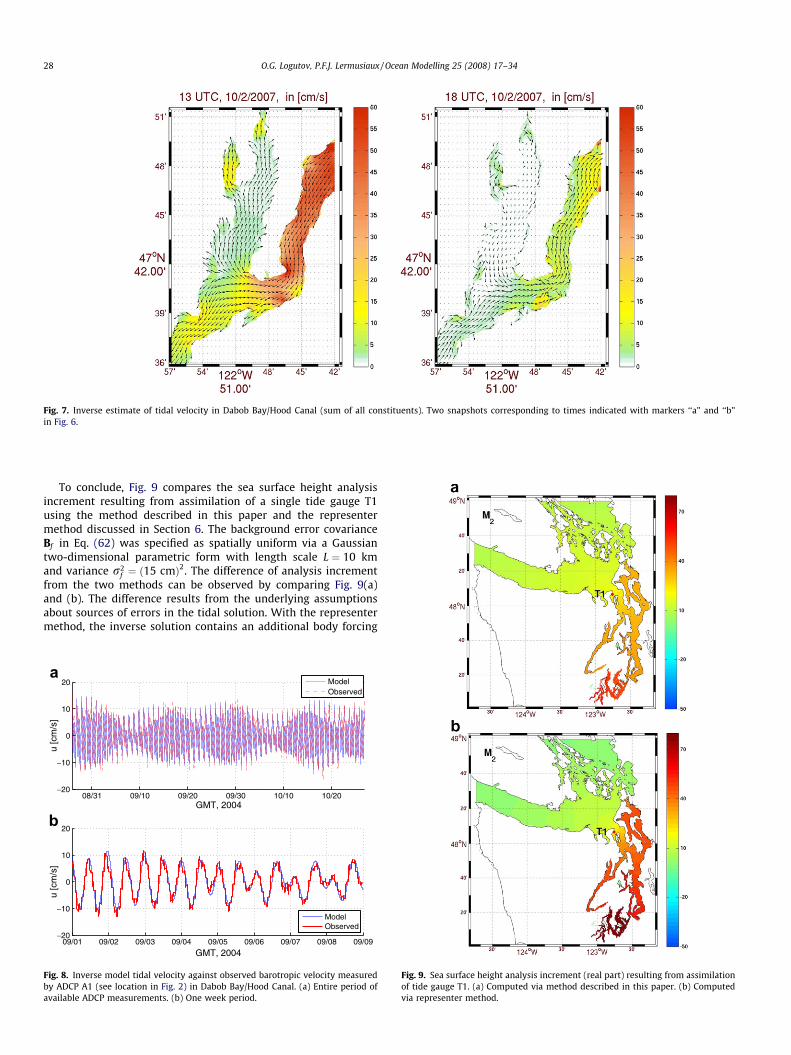
Fig. 7. Inverse estimate of tidal velocity in Dabob Bay/Hood Canal (sum of all constituents). Two snapshots corresponding to times indicated with markers ‘‘a” and ‘‘b”in Fig. 6.

28 O.G. Logutov, P.F.J. Lermusiaux / Ocean Modelling 25 (2008) 17–34

To conclude, Fig. 9 compares the sea surface height analysisincrement resulting from assimilation of a single tide gauge T1using the method described in this paper and the representermethod discussed in Section 6. The background error covarianceBf in Eq. (62) was specified as spatially uniform via a Gaussiantwo-dimensional parametric form with length scale L ¼ 10 kmand variance r2

f ¼ ð15 cmÞ2. The difference of analysis incrementfrom the two methods can be observed by comparing Fig. 9(a)and (b). The difference results from the underlying assumptionsabout sources of errors in the tidal solution. With the representermethod, the inverse solution contains an additional body forcing

08/31 09/10 09/20 09/30 10/10 10/20−20

−10

0

10

20

GMT, 2004

u [c

m/s

]

ModelObserved

09/01 09/02 09/03 09/04 09/05 09/06 09/07 09/08 09/09−20

−10

0

10

20

GMT, 2004

u [c

m/s

]

ModelObserved

a

b

Fig. 8. Inverse model tidal velocity against observed barotropic velocity measuredby ADCP A1 (see location in Fig. 2) in Dabob Bay/Hood Canal. (a) Entire period ofavailable ADCP measurements. (b) One week period.

Fig. 9. Sea surface height analysis increment (real part) resulting from assimilationof tide gauge T1. (a) Computed via method described in this paper. (b) Computedvia representer method.

O.G. Logutov, P.F.J. Lermusiaux / Ocean Modelling 25 (2008) 17–34 29

term (Eq. (62)) that originates from an assumption about tidalmodel errors. With the method presented in this paper, the inversesolution is constructed following a proposition that largest errorsoften originate from the open boundary conditions and the inversesolution is such that it satisfies the barotropic tidal dynamics ex-actly. In our own practice of regional tidal modeling, the latter ap-proach was found to be somewhat more robust and practical.

8. Conclusions

A new methodology and computational system for forward andinverse barotropic tidal modeling for regional tidal estimation havebeen developed. The modeling system is capable of forward (nodata assimilation) tidal field predictions over high resolutionbathymetry, and subsequent assimilation of tidal elevation andvelocity observational data via a new practical inverse method.The forward prognostic scheme solves the linearized depth-inte-grated shallow water equations as a boundary value problem inthe spectral domain. The inverse scheme assimilates filtered tidalvelocity observations by adjusting the OBCs. After assimilation,the interior and boundary tidal fields are in accord with the tidalmodel and with the error covariances of the tidal observationsand the prior OBC estimate. With this methodology and computa-tional system, we have carried out accurate barotropic tidal fieldestimations for multi-scale nested domains including complex in-land waterways is several regions of the world’s oceans. To illus-trate our results, such a computation was presented in the areaof Dabob Bay and Hood Canal, WA.

The inverse procedures are specifically designed for regionalocean applications. We found that both high resolution and controlof the barotropic model through OBCs are important elements insuccessful regional tidal modeling. This is because the tidal forcingis provided through the OBCs in regional ocean applications andcan constitute a significant source of uncertainty. To reduce theseuncertainties, the prior tidal conditions at the open boundariesneed to be adjusted to the observational data, high-resolutionbathymetry, and tidal dynamics. Our tidal model is fitted to datathrough a correction made to OBCs, consistent with the errorcovariances of the data and the prior OBCs. The inverse solutiongenerated by our method presently satisfies the barotropic shallowwater dynamical equations exactly.

The data assimilation scheme developed in this paper differsfrom previous techniques mostly by our use of a spectral-domainshallow water model and our implementation of a new inversewhich is practical and does not require an adjoint model. In ourmethod, an optimization is carried out in the OBC space rather thanin the observational space or model state space as is the practice inother popular tidal data assimilation and inversion methods (e.g.,representer approach, nudging, optimal interpolation, etc). Ourstrategy is motivated by the specifics of regional tidal modelingapplications, in which the OBCs constitute a significant source ofuncertainty. Our methodology and computational system are ex-pected to continue to find wide-range applications in regional andcoastal ocean science, including the estimation of barotropic tidalforcing needed for regional primitive equation modeling systems.

Variations of our approach and computational system can, ofcourse, be further developed. For example, specific model fieldand parameter uncertainties can be included in the interior to ac-count for non-linear effects and uncertainties of shallow watermodel parameters (e.g., bottom drag). The Error Subspace Statisti-cal Estimation (ESSE) approach (Lermusiaux, 2002; Lermusiaux,2006) can be additionally utilized to efficiently represent modelfield uncertainties at interior ocean nodes by their dominant eigen-modes. This would allow us to continue to provide timely tidalestimates in varied regions of the worlds coastal ocean. The inverse

scheme could also be upgraded to include a multi-model fusion ap-proach, with 2-D and 3-D barotropic tidal models combined to-gether to produce the highest possible horizontal resolution, onthe one hand, and resolution of the vertical velocity structureand boundary layers, on the other (Logutov, 2007). Future workcould also include the implementation of our forward and inversemodel on an Arakawa-B grid to add consistency with Arakawa-Bformulated primitive equation models utilizing barotropic tidalforcing. Our presently linear forward modeling scheme can alsobe extended to a nonlinear predictor using a perturbation methodand an iterative procedure, as described in Section 2. The OBCs ofthis nonlinear model could then be corrected at each iterationusing tidal data and our inversion scheme. Finally, the fusion ofthe barotropic model with baroclinic tidal and internal wave mod-els might be desirable. All together, these extensions could lead tohighly accurate, data-driven barotropic and baroclinic tidal model-ing at highest resolutions.

Acknowledgements

This research was supported in part by the Office of Naval Re-search under grants PLUSNet (S05-06), AWACS (N00014-07-1-0501) and MURI-ASAP (N00014-04-1-0534). We thank Dr. PatrickJ. Haley, Jr. for useful discussions and Wayne Leslie for the manage-ment of tidal observations. We also thank the whole PLUSNet-07(PN07) team for their collaboration and feedback before and duringPN07. We are grateful to Edward G. Josberger of the US GeologicalSurvey who has provided us with the ADCP data obtained in theHood Canal in September-October of 1994. We would also like tothank the anonymous reviewers of this paper for their timely re-sponse and constructive suggestions and criticisms.

This is with great sadness that we learned that Prof. Peter Kill-worth, the founder and the Editor-in-Chief of Ocean Modelling fromjournals’ inception in 1999, has passed away on the day of subm-ition of this paper. We would like to acknowledge exceptional sci-entific and editorial contributions of Prof. Killworth made to thefield of physical oceanography and ocean modeling and expressour sincere condolences to his family and close friends.

Appendix A. Notation

A 2 Cm�n complex m� n matrix,N

a 2 C complex vector of length N,

K a diagonal matrix,AH transposed and complex conjugated A,A�H an inverse of AH ,ðAÞj the ðjÞth column of A,ðAÞi;j the ði; jÞth entry of A,ðaÞi the ith entry of a,N a set of natural numbers f1;2; . . .g,iK 2 NK a set iK ¼ fikgK

k¼1, ik 2 f1;2; . . .g,ðaÞiK

2 CK comlex vector of length K containing the iK th entriesof a, ðaÞiK

¼ ½ai1 ; ai2 ; . . . ; aiK �T ,

ðAÞiK ;jL2 CK�L comlex K � L matrix containing the entries in the

iK th rows and jLth columns of matrix A,

ðAÞiK ;jL¼

ai1 ;j1 ai1 ;j2 . . . ai1 ;jL

ai2 ;j1 ai2 ;j2 . . . ai2 ;jL

..

. . ..

. . . ...

aiK ;j1 aiK ;j2 . . . aiK ;jL

266664

377775

K�L

;

vecðAÞ the vector version of A obtained by rearranging the col-umns to a vector, i.e. vecðAÞ ¼ ½aT

1; aT2; . . . ; aT

n�T,

Ocean Modelling 25 (2008) 17–34

0N the null vector of length N (all entries are zero),1 the ones vector of length N (all entries are one),

N

A B the Hadamard (elementwise) product of A and B,AøB the Hadamard (elementwise) division of A by B, with spe-cial definition for zero elements in B

ðAøBÞi;j ¼ ðAÞi;j=ðBÞi;j if ðBÞi;j 6¼ 0;ðAøBÞi;j ¼ 0 if ðBÞi;j ¼ 0;

ðA:1Þ

30 O.G. Logutov, P.F.J. Lermusiaux /

DðaÞ 2 CN�N diagonal N � N matrix with vector a 2 CN specify-ing the main diagonal, ðDðaÞÞ ¼ di;jai,

i;j i�1;j i;j i;jþ1 i�1;jþ1

i;j

D�nðaÞ 2 CN�N diagonal N � N matrix with vector a 2 CN speci-fying the ð�nÞth (lower) diagonal, such that ðD�nðaÞÞi;j ¼ di�n;jai,DþnðaÞ 2 CN�N diagonal N � N matrix with vector a 2 CN speci-fying the ðþnÞth (upper) diagonal, such that ðDþnðaÞÞi;j ¼ diþn;jai,DþnðaÞ ¼ DT

�nðaÞ and DðaÞ ¼ D�0ðaÞ ¼ Dþ0ðaÞ,

Appendix B. Specifics of model implementation

Below, we provide details on specification of matricesGu g, Gv g, Fu u, Fu v, Fv u, Fv v, Dg u, Dg v, Hu u, andHv v utilized in forming the discrete model operators (21),(22), and (26).

B.1. Grids, masks, and bottom topographies

The Arakawa-C staggered grid, with the schematic given in Fig.1, is utilized throughout. The coordinate of each grid point is iden-tified in terms of latitude and longitude stored in Ugrid;Kgrid 2 Rm�n

(lat,lon) for g;u; v-grids. Firstly, a land mask, Mg, is defined at g gridpoints. The mask is a logical array of size m� n, with entries set atocean grid points and unset at masked/land points. The land masksfor u and v grids, Mu and Mv, are derived from Mg by unsetting theentries of the u,v nodes neighboring with masked g nodes, viz inFig. 1, the filled symbols which indicate masked g;u; v-nodes. Letmgrid denote the vectorized model grid matrix, Mgrid, i.e.,mgrid ¼ vecðMgridÞ, where grid ¼ fg; u; vg.

The model does not put any restrictions on the steepness of bot-tom topography. However, if this inverse barotropic model is exer-cised in conjunction with a primitive equation model, the bottomtopographies at their open boundaries should be consistent. LetHg 2 Rm�n denote the values of bottom topography at g-gridpoints, positive for ocean nodes. The bottom topography at u andv grids, Hu;Hv 2 Rm�n are needed in (26). On an Arakawa-C grid,this is computed from Hg following

Hui;j ¼ ðH

gi;j þ Hg

i;j�1Þ=ðMgi;j þMg

i;j�1Þ if Mui;j ¼ 1

Hui;j ¼ 0 if Mu

i;j ¼ 0

Hvi;j ¼ ðH

gi;j þ Hg

i�1;jÞ=ðMgi;j þMg

i�1;jÞ if Mvi;j ¼ 1

Hvi;j ¼ 0 if Mv

i;j ¼ 0:

ðB:1Þ

With hgrid ¼ vecðHgridÞ, the operators

Hu u ¼ DðhuÞ; Hv v ¼ DðhvÞ ðB:2Þ

define mappings from tidal velocities to transports (26) on u and vgrids, respectively. Note that mappings u g and v g are givenby backward differences and mappings g u and g v by forwarddifferences on an Arakawa-C grid. We zero-pad the boundary ele-ments to maintain m� n dimensionality of matrices.

B.2. Gradient and divergence operators

On a staggered Arakawa-C grid, the forward difference operatorsin the zonal x and meridional y directions

Dfrwdk ¼ Dþmð1NÞ �Dð1NÞ

Dfrwd/ ¼ Dþ1ð1NÞ �Dð1NÞ

ðB:3Þ

define the mappings from the u and v grids onto the g grid (sche-matic in Fig. 1), while the backward difference operators

Dbcwdk ¼ Dð1NÞ �D�mð1NÞ

Dbcwd/ ¼ Dð1NÞ �D�1ð1NÞ

ðB:4Þ

define mappings from g-grid onto u and v grids, respectively. Thus,the gradient operator g$f�g in (19) which maps from g to u and vgrid-points is implemented via backward differences

Gu g ¼ Dðgu gÞDbcwdk

Gv g ¼ Dðgv gÞDbcwd/

ðB:5Þ

where the diagonal matrices Dðgu gÞ and Dðgv gÞ correspond tometric terms in g$f�g (g is acceleration due to gravity):

gu g ¼ g � ð1Nødku gÞ

gv g ¼ g � ð1Nød/v gÞ;

ðB:6Þ

where dku g, d/

v g represent metric terms on a spherical grid. Simi-larly, the divergence operator (24) maps from u and v to g grid-points and is implemented via forward differences

Dg u ¼ Dðdg uÞDfrwdk

Dg v ¼ Dðdg vÞDfrwd/

ðB:7Þ

where the diagonal matrices Dðdg uÞ and Dðdg vÞ correspond tometric factors in $ � fg:

dg u ¼mgødkg u

dg v ¼mgød/g v

ðB:8Þ

Since dg u and dg v contain the mask mg, the multiplicationsðDg uuÞ and ðDg vvÞ produce zero values at masked g points forany values of u and v, that is ðDg uuÞig

mask¼ 0ng

maskand

ðDg vvÞigmask¼ 0ng

mask.

B.3. Rotational operators

Operators Fu v and Fv u in (20) map across the u; v staggeredgrids. The computations of their components are now described.First, the averaging operators are computed. On an Arakawa-C grid,a four-point stencil of v-points around an ði; jÞth u-node leads to

vui;j ¼ðMv

i;j�1vi;j�1 þMviþ1;j�1viþ1;j�1 þMv

iþ1;jviþ1;j þMvi;jvi;jÞ

ðMvi;j�1 þMv

iþ1;j�1 þMviþ1;j þMv

i;jÞðB:9Þ

interpolation rule from v to u grid. In the foregoing, vui;j is the value

of the ði; jÞth element of v interpolated to the ði; jÞth u-grid pointfrom its corresponding four-point v-grid stencil (vu

i;j set to zero ifall the mask values in the denominator are zero). Similarly, afour-point stencil of u-points around an ði; jÞth v-node leads to

uvi;j ¼ðMu

i�1;jui�1;j þMui;jui;j þMu

i;jþ1ui;jþ1 þMui�1;jþ1ui�1;jþ1Þ

ðMui�1;j þMu

i;j þMui;jþ1 þMu

i�1;jþ1ÞðB:10Þ

interpolation rule from u to v grid (again, uvi;j set to zero if all the

mask values in the denominator are zero). In order to implement(B.9) and (B.10) in terms of averaging operators Su v and Sv u actingon vectors defined on the v and u grids, respectively, we form thematrices Nu and Nv corresponding to the denominator in (B.9) and(B.10)

ðNÞui;j ¼ ðMÞvi;j�1 þ ðMÞ

viþ1;j�1 þ ðMÞ

viþ1;j þ ðMÞ

vi;j

ðNÞv ¼ ðMÞu þ ðMÞu þ ðMÞu þ ðMÞuðB:11Þ

O.G. Logutov, P.F.J. Lermusiaux / Ocean Modelling 25 (2008) 17–34 31

and denote nu ¼ vecðNuÞ and nv ¼ vecðNvÞ. The four-point averagingoperators Su v and Sv u in (B.9) and (B.10) are then obtained as(symbol definitions are in Appendix A)

~Su v ¼ D�mðmvÞ þD�mþ1ðmvÞ þDðmvÞ þDþ1ðmvÞ~Sv u ¼ D�1ðmuÞ þDðmuÞ þDm�1ðmuÞ þDþmðmuÞSu v ¼ Dð1NønuÞ~Su v

Sv u ¼ Dð1NønvÞ ~Sv u

ðB:12Þ

Second, the values of the determinant (14) and other frequencyelements are computed as follows. With vectors jgrid; fgrid 2 RN

containing the friction and Coriolis coefficients at model grid-points (ð:Þgrid denotes specific staggered grid, either fg;u; vg) andx denoting the tidal constituent frequency, this determinant(14) is,

qgrid ¼ ðix � 1N þ jgridÞ ðix � 1N þ jgridÞ þ fgrid fgrid ðB:13Þ

and the vector frequency elements are

xu ¼mu ðix � 1N þ juÞøqu

xv ¼mv ðix � 1N þ jvÞøqv

fu ¼mu fuøqu

fv ¼ �mv fvøqv

ðB:14Þ

The operator matrices Fu u and Fv v 2 RN�N defining mappingsu u and v v in (20) are then obtained from xgrid (B.14) as

Fu u ¼ DðxuÞFv v ¼ DðxvÞ

ðB:15Þ

The operator matrices Fu v and Fv u in (20) defining mappingsu v and v u across the staggered u and v grids are then finallyobtained from fgrid (B.14) by utilizing the four-point stencil averag-ing operators (B.12)

Fu v ¼ DðfuÞSu v

Fv u ¼ DðfvÞSv uðB:16Þ

Matrices Fu v and Fv u 2 RN�N are four-diagonal. Note that because(B.14) contains the masks mu and mv, the operators (B.15) and(B.16) produce zero velocity values at masked u and v points.

Appendix C. Optimal OBC increment

Here, we provide the derivation of (47). Consider the problem offinding optimal OBCs

gobc ¼ arg ming

JðgobcÞ; ðC:1Þ

with the penalty functional

JðgobcÞ ¼ ðgobc � g�obcÞHB�1

obcðgobc � g�obcÞ þ ðy �HxÞHR�1ðy �HxÞ:ðC:2Þ

where g�obc is the a-priori OBC estimates, matrices Bobc and R are OBCand observational error covariances, and state-space x is given by

x ¼Mðx gobcÞgobc: ðC:3Þ

Eqs. (C.1)–(C.3) are equivalent to (45), (46), and (44).

Theorem 1. The minimization problem C.1, C.2, C.3 has a uniquesolution given by

gobc ¼g�obc þ BobcMHðx gobcÞH

HðHMðx gobcÞBobcMHðx gobc ÞH

H þ RÞ�1

� ðy �HMðx gobcÞg�obcÞ: ðC:4Þ

Proof. Since matrices Bobc and R are covariances and, therefore,symmetric and positive definite, the quadratic penalty function(C.2) is convex and has a unique minimum. The minimum can befound in closed form by expressing the gradient of JðgobcÞ withrespect to gobc

rJðgobcÞ ¼ B�1obcðgobc � g�obcÞ �MH

ðx gobcÞHHR�1ðy

�HMðx gobcÞgobcÞ ðC:5Þ

and setting it to zero

rJðgobcÞ ¼ 0: ðC:6Þ

By solving (C.6) for gobc , we obtain

gobc ¼ ðB�1obc þMH

ðx gobcÞHHR�1Mðx gobcÞHÞ

�1B�1obcg

�obc þ ðB

�1obc

þMHðx gobcÞH

HR�1Mðx gobc ÞHÞ�1MH

ðx gobcÞHHR�1y ðC:7Þ

We next apply the Sherman-Morrison-Woodbury identity

ðB�1 þ UHR�1VÞ�1 ¼ B� BUHðVBUH þ RÞ�1VB ðC:8Þ

to the first term in (C.7) and the identity

ðB�1 þ UHR�1VÞ�1UHR�1 ¼ BUHðVBUH þ RÞ�1 ðC:9Þ

to the second term in (C.7).Identities (C.8) and (C.9) are valid for any matrices B, R, U, V of

correct sizes. The validity of the Sherman-Morrison-Woodburyformula can be shown by multiplying B�1 þ UHR�1V with theright-hand side of (C.8) and showing that the result is identity. Eq.(C.9) is a corollary of (C.8) shown as lemma 1 below. By using theidentities (C.8) and (C.9) with U ¼ V ¼Mðx gobcÞH in (C.7), weobtain (C.4). h

Lemma 1. (C.9) holds for any matrices B, R, U, V of correct sizes.

Proof.. Let Q denote

Q � VBUH þ R

By (C.8)

ðB�1 þ UHR�1VÞ�1UHR�1 ¼ BUHR�1 � BUHðVBUH þ RÞ�1VBUHR�1

¼ BUHðQ�1QR�1 � Q�1VBUHR�1

¼ BUHQ�1ððVBUH þ RÞR�1 � VBUHR�1Þ

¼ BUHQ�1: �

Appendix D. Conversion between time and spectral domains

D.1. Preliminaries

Tidal harmonic constants at tide gauges are typically tabulatedfollowing the standard convention as either an amplitude, jujk, anda Greenwich phase, ju

k , for each tidal constituent k, i.e., a tupleðjukj;ju

kÞ, or as a complex amplitude uk

uk ¼ jukje�ijuk : ðD:1Þ

Variable u in the foregoing represents either an SSH (g), or a zonal(u) or meridional (v) component of tidal velocity. Note the minussign for Greenwich phases in (D.1), ju

k ¼ �\uk, which is a universalconvention. For a given tidal constituent k, every moment in timemaps to an astronomical phase hk. An astronomical phase of a tidalconstituent k at UTC time tUTC

0 can be obtained using astronomicaltables or a t_tide toolbox implemented in matlab by Pawlowiczet al. (2002). The tidal time series is recovered from tidal harmonicconstants ðjukj;ju

kÞ as

32 O.G. Logutov, P.F.J. Lermusiaux / Ocean Modelling 25 (2008) 17–34

utideðtÞ ¼Xq

k¼1

jukj cosðxkt þ hk � jukÞ ðD:2Þ

or from complex uk in (D.1) as

utideðtÞ ¼ RXq

k¼1

uk exp iðxkt þ hkÞ( )

ðD:3Þ

where hk is an astronomical phase at time t ¼ 0. We also note thatGreenwich phases ju

k are typically given corresponding to local timezones and care should be taken to ensure that time t and ju

k areconsistent.

D.2. Velocity data

The time series of zonal and meridional velocity components uand v at point ðxi; yiÞ are reconstructed from the spectral domainvariables ~uk and ~vk following (8), which is equivalent to

utideðtÞ ¼Xq

k¼1

~uk

2exp iðxkt þ hkÞ þ

~uk2

exp iðxkt þ hkÞ�

ðD:4Þ

vtideðtÞ ¼Xq

k¼1

~vk

2exp iðxkt þ hkÞ þ

~vk2

exp iðxkt þ hkÞ�

ðD:5Þ

where ~uk and ~vk denote complex conjugates of ~uk and ~vk. In order tofacilitate velocity data analysis, define a complex variable

UðtÞ � uðtÞ þ i vðtÞ ðD:6Þ

with the real and imaginary parts given by the zonal and meridionalvelocity components. As directly seen from (D.4) and (D.5), thecomplex velocity UkðtÞ associated with each tidal constituent k isdescribed as a sum of counter-clockwise rotating (~ak) and clockwiserotating (~a�k) complex exponents

UkðtÞ � ukðtÞ þ i vkðtÞ ¼ ~akeiðxktþhkÞ þ ~a�ke�iðxktþhkÞ; ðD:7Þ

with the complex amplitudes ~ak and ~a�k given by

~ak ¼~uk þ i~vk

2; ~a�k ¼

~uk þ i~vk2

: ðD:8Þ

Eq. (D.7) describes an ellipse in a complex plane, with the counter-clockwise rotation of velocity vectors if j~akj > j~a�kj and clockwiserotation if j~akj < j~a�kj. A velocity vector at any given moment of timeis a superposition of two circular components, the first and the sec-ond terms on the right-hand-side of (D.7), rotating in the positive(counter-clockwise) and negative (clockwise) directions, respec-tively. The maximum current occurs when the circular componentshave the same phase, i.e., the positively and negatively rotating ra-dial vectors point in the same direction. In this case, their velocitymagnitudes are added and the current velocity is

Mk ¼ j~akj þ j~a�kj: ðD:9Þ

Mk is the length of the major semi-axis of a velocity ellipse. Theminimum current occurs when the circular components have180� phase difference. In this case, the current velocity is

mk ¼ j~akj � j~a�kj; ðD:10Þ

positive for the counter-clockwise and negative for clockwise veloc-ity vector rotation. Thus, the magnitude of mk is the length of theminor semi-axis of a velocity ellipse. A velocity ellipse degeneratesinto a line when j~akj ¼ j~a�kj. The oppositely rotating radial vectorsrepresenting the two terms on the right-hand-side of (D.7) meet(generate maximum current) at an angle

/k ¼ ð\ð~a�kÞ þ \ð~akÞÞ=2 ðD:11Þ

(\ denotes an argument of a complex number). Therefore, (D.11)provides an inclination of the major semi-axis, also referred to as el-

lipse inclination. The northern major semi-axis is typically utilized asthe reference axis and, therefore, 180 is subtracted from /k, if/k > 180. The Greenwich phase is defined as an angle that thetwo oppositely rotating radial vectors have to traverse from theirinitial positions, ðxkt þ hkÞ ¼ 0, before they meet each other, i.e.,an angle between an initial position and the first encountered majorsemi-axis for either of the oppositely rotating radial vectors. Simplealgebra reveals that this angle is given by

gk ¼ ð\ð~a�kÞ � \ð~akÞÞ=2: ðD:12Þ

Greenwich phase gk describes a delay, Dt ¼ gk=xk, of the maximumcurrent relative to the zero astronomical phase times (i.e., momentsof time when ðxkt þ hkÞ ¼ 0). By solving (D.8) for uk and vk, we canobtain the tidal harmonics in terms of the exponent coefficients

uk ¼ ~ak þ ~a�k; vk ¼ ið~a�k � ~akÞ ðD:13Þ

where ~a�k is the conjugate of ~a�k.

D.3. Harmonic analysis

Arrange observational data as a complex vector zobs 2 Cnt

zobs ¼ uobs þ ivobs ðD:14Þ

with uobs and vobs 2 Rnt containing either the zonal and the meridi-onal components of the observed currents or the observed sea sur-face height, in which case only the real part uobs is needed. The timetUTC of measurements zobs referenced at tUTC

0 is arranged in a vectortobs 2 Rnt , i.e.,

tobs ¼ tUTC � tUTC0 1nt : ðD:15Þ

The astronomical phase hk corresponding to tUTC0 can be obtained by

using t_tide toolbox of Pawlowicz et al. (2002). Also, let columnvector xq 2 Rq;2q < nt denote tidal constituent frequencies.

We seek a least-squares fit of tidal constituents (D.4) and (D.5)to observational data zobs. Least-squares analysis can be carried byspecifying the basis matrix

Ent�2q � ½Eþnt�q; E�nt�q�; ðD:16Þ

corresponding to (D.7), with

Eþnt�q ¼ expði tnt xTqÞ; Eþnt�q ¼ expð�i tnt x

TqÞ

where exp denotes an entry-wise exponential (not a matrix expo-nential). By minimizing the squares of the misfits

a ¼ arg mina

JðaÞ

JðaÞ ¼ ðzobs � En�2qaÞHðzobs � En�2qaÞðD:17Þ

as a function of coefficients a (e.g., using the method of Lagrangemultipliers), we obtain

a ¼ ðEHEÞ�1EHzobs ðD:18Þ

Partition a into coefficients corresponding to Eþnt�q and E�nt�q

a ¼aþ

a�

� �2q

ðD:19Þ

with aþ and a� 2 Cq. Values of coefficients aþ and a� depend on thereference time utilized in the harmonic analysis procedures. Refer-ence time is related to the astronomical phase hk via (D.7). There-fore, we can obtain the tidal constants ~aþk and ~a�k independent ofthe reference time in the harmonic analysis by absorbing hk intothe constants

~ak ¼ ak expð�ihkÞ; ~a�k ¼ a�k expðihkÞ ðD:20Þ

where ak ¼ ðaþobsÞk and a�k ¼ ða�obsÞk. With ~aþk and ~a�k, the values ofcomplex amplitudes ~uk and ~vk in (8) are obtained following (D.13).

O.G. Logutov, P.F.J. Lermusiaux / Ocean Modelling 25 (2008) 17–34 33

References

Andersen, O., Egbert, G., Erofeeva, S., Ray, R., 2006. Mapping nonlinear shallow-water tides: a look at the past and future. Ocean Dyn. 56, 416–429. 14.

Baines, P.G., 1982. On internal tide generation models. Deep Sea Res. A 29 (3), 307–338.

Bennett, A., McIntosh, P., 1982. Open ocean modeling as an inverse problem: Tidaltheory. J. Phys. Oceanogr. 12, 1004–1018.

Bennett, A.F., 1992. Inverse Methods in Physical Oceanography. CambridgeMonographs on Mechanics and Applied Mathematics. Cambridge UniversityPress, Cambridge.

Bennett, A.F., 2002. Inverse Modeling of the Ocean and Atmosphere. CambridgeUniversity Press, Cambridge.

Bernard, P.E., Remacle, J.F., Legat, V., 2008. Boundary dicretization for high orderdiscontinuous Galerkin computations of tidal flows around shallow waterislands. Int. J. Numer. Methods Fluids, doi:10.1002/fld.1831.

Besiktepe, S.T., Lermusiaux, P.F.J., Robinson, A.R., 2003. Coupled physical andbiochemical data driven simulations of massachusetts bay in late summer: real-time and post-cruise data assimilation. In: Gregoire, M., Brasseur, P.,Lermusiaux, P. (Eds.), Special issue on The use of data assimilation in coupledhydrodynamic, ecological and bio-geo-chemical models of the oceans. Vol. 40. J.Mar. Syst. pp. 171–212.

Blain, C., Preller, R., Rivera, A., 2002. Tidal prediction using the advanced circulationmodel (ADCIRC) and a relocatable PC-based system. Oceanography 15 (1), 77–87.

Blayo, E., Debreu, L., 2005. Revisiting open boundary conditions from the point ofview of characteristic variables. Ocean Modell. 9 (3), 231–252.

Canizares, R., Madsen, H., Jensen, H., Vested, H., 2001. Developments inoperational shelf sea modelling in Danish waters. Estuar. Coast. Shelf Sci. 53,595–605.

Chapman, D., 1985. Numerical treatment of cross-shelf open boundaries in abarotropic coastal ocean model. J. Phys. Oceanogr. 15, 1060–1075.

Chen, C., Beardsley, R., 1998. Tidal mixing and cross-frontal particle exchange over afinite amplitude asymmetric bank: a model study with application to GeorgesBank. J. Mar. Res. 56, 1163–1201.

Das, S.K., Lardner, R.W., 1992. Variational parameter estimation for a two-dimensional numerical tidal model. Int. J. Numer. Methods Fluids 15, 313–327.

Davies, A.M., 1993. A bottom boundary layer-resolving three-dimensional tidalmodel: a sensitivity study of eddy viscosity formulation. J. Phys. Oceanogr. 23,1437–1453.

Davies, A.M., Gerritsen, H., 1994. An intercomparison of three dimensional tidalhydrodynamic models of the Irish sea. Tellus 46A, 200–221.

Davies, A.M., Jones, J.E., Xing, J., 1997a. Review of recent developments in tidalhydrodynamic modelling I. Spectral models. J. Hydrol. Eng. ASCE 123, 278–292.

Davies, A.M., Jones, J.E., Xing, J., 1997b. Review of recent developments in tidalhydrodynamic modelling II: turbulence energy models. J. Hydrol. Eng. ASCE123, 293–302.

Davies, A.M., Kwong, S.C.M., Flather, R.A., 1997c. A three dimensional model ofdiurnal and semi-diurnal tides on the European shelf. J. Geophys. Res. 102,8625–8656.

Davies, H.C., 1976. A lateral boundary formulation for multi-level predictionmodels. Quart. J. R. Met. Soc. 102, 405–418.

Dee, D.P., 1995. On-line estimation of error covariance parameters for atmosphericdata assimilation. Monthly Weather Rev. 123, 1128–1145.

Egbert, G., Bennett, A., Foreman, M. 1994. TOPEX/Poseidon tides estimated using aglobal inverse model. J. Geophys. Res. 99, C12, 24, 821, 24,852.

Egbert, G., Erofeeva, S., 2002. Efficient inverse modeling of barotropic ocean tides. JAtmos. Ocean. Technol. 19, 183–204.

Egbert, G.D., 1997. Tidal data inversion: interpolation and inference. Progr.Oceanogr. 40, 53–80.

Evangelinos, C., Lermusiaux, P.F.J., Geiger, S.K., Chang, R.C., Patrikalakis, N.M., 2006.Web-enabled configuration and control of legacy codes: an application to oceanmodelling. Ocean Modell. 13, 197–220.

Flather, B., 1976. A tidal model of the northwest European continental shelf. Mem.Soc. R. Sci. Liege 10, 141–164.

Foreman, M.G.G., Thomson, R.E., 1997. Three dimensional model simulations oftides and buoyancy currents along the west coast of Vancouver island. J. Phys.Oceanogr. 27, 1300–1325.

Franks, P., Chen, C., 1996. Plankton production in tidal fronts: a model of GeorgesBank.

Garrett, C., Gerkema, T., 2007. On the body-force term in internal-tide generation. J.Phys. Oceanogr. 37, 2172–2175.

George, K., 2007. A depth-averaged tidal numerical model using non-orthogonalcurvilinear co-ordinates. Ocean Dyn. 57, 363–374.

Greenberg, D.A., Shore, J.A., Page, F.H., M., D., 2005. A finite element circulationmodel for embayments with drying intertidal areas and its application to thequoddy region of the bay of fundy. Ocean Modell. 10, 211–231.

Grenier, R.R., Luettich, R.A., Westerin, J.J., 1995. A comparison of non-linearfrictional characteristics of two-dimensional and three-dimensional models ofa shallow tidal embayment. J. Geophys. Res. 100, 13719–13735.

Haley, Jr., P.J., Lermusiaux, P.F.J., Robinson, A.R., Leslie, W.G., Logutov, O.,Cossarini, G., Liang, X.S., Moreno, P., Ramp, S.R., Doyle, J., Bellingham, J.,Chavez, F., Johnston, S., in press. Forecasting and reanalysis in the MontereyBay/California current region for the Autonomous Ocean Sampling Network-IIExperiment. Deep Sea Res., Part II.

He, R., Wilkin, J.L., 2006. Barotropic tides on the southeast new england shelf: a viewfrom a hybrid data assimilative modeling approach. J. Geophys. Res. 111,C08002.

Hea, Y., Lub, X., Qiua, Z., Zhaoc, J., 2004. Shallow water tidal constituents in theBohai Sea and the Yellow Sea from a numerical adjoint model with TOPEX/POSEIDON altimeter data. Cont. Shelf Res. 24, 1521–1529.

Heemink, A., Kloosterhuis, H., 1990. Data assimilation for non-linear tidal models.Int. J. Numer. Methods Fluids 11 (12), 1097–1112.

Hubbert, G.D., Preller, R., P.G. Posey, G., Carroll, S., 2001. Software requirementsspecification for the globally relocatable navy tide/atmosphere modelingsystem (PCTides). Memorandum Report NRL/MR/7322-01-8266, NavalResearch Laboratory, Stennis Space.

Jones, J.E., Davies, A.M., 1996. A high resolution three dimensional model of theM2,M4, M6, S2, N2, K1 and O1 tides in the eastern Irish Sea. Estuar. Coast. Shelf Sci.42, 311–346.

Kurapov, A., Egbert, G., Allen, J., Miller, R., Erofeeva, S., Kosro, P., 2003. M2 internaltide off Oregon: inferences from data assimilation. J. Phys. Oceanogr. 33, 1733–1757.

Kurapov, A.L., Egbert, G.D., Allen, J.S., Miller, R.N., 2007. Representer-basedvariational data assimilation in a nonlinear model of nearshore circulation. J.Geophys. Res. 112, C11019.

Lavelle, J., Thacker, W., 2008. A pretty good sponge: dealing with open boundaries inlimited-area ocean models. Ocean Modell. 20, 270–292.

Le Cann, B., 1990. Barotropic tidal dynamics of the bay of biscay shelf. Cont. ShelfRes. 10 (8), 723–758.

Lee, J., Jung, K., 1999. Application of eddy viscosity closure models for the M2 tideand tidal currents in the Yellow sea and the East China sea. Cont. Shelf Res. 19(4), 445–475.

LeProvost, C., Genco, M.L., Lyard, F., Vincent, P., Canceil, P., 1994. Spectroscopy of theworld ocean tides from a finite element hydrodynamic model. J. Geophys. Res.99(C12), 24777–24798.

LeProvost, C., Rougier, G., Poncet, A., 1981. Numerical modeling of the harmonicconstituents of the tides, with application to the English channel. J. Phys.Oceanogr. 11, 1123–1138.

LeProvost, C., Vincent, P., 1986. Some tests of precision for a finite element model ofocean tides. J. Comput. Phys. 65, 273–291.

Lermusiaux, P.F.J., 1997. Error subspace data assimilation methods for ocean fieldestimation: theory, validation and applications (Harvard Ocean PredictionSystem). Ph.D. thesis, Harvard University.

Lermusiaux, P.F.J., 1999. Data assimilation via error subspace statistical estimation.part II: Mid-atlantic bight shelfbreak front simulations, and esse validation.Monthly Weather Rev. 127 (8), 1408–1432.

Lermusiaux, P.F.J., 2002. On the mapping of multivariate geophysical fields:sensitivity to size, scales and dynamics. J. Atmos. Ocean. Technol. 19, 1602–1637.

Lermusiaux, P.F.J., 2006. Uncertainty estimation and prediction for interdisciplinaryocean dynamics. J. Comput. Phys. 217, 176–199.

Lermusiaux, P.F.J., 2007. Adaptive modeling, adaptive data assimilation andadaptive sampling. Physica D 230, 172–196.

Lermusiaux, P.F.J., Anderson, D.G., Lozano, C.J., 2000. On the mapping of multivariategeophysical fields: error and variability subspace estimates. Quart. J. R. Met.Soc., 1387–1430.

Lermusiaux, P.F.J., Chiu, C.-S., 2002. Four-dimensional data assimilation for coupledphysical-acoustical fields. In: Pace, N., Jensen, F. (Eds.), Acoustic Variability.Kluwer, Academic Press, pp. 417–424.

Lermusiaux, P.F.J., Chiu, C.S., Gawarkiewicz, G.G., Abbot, P., Robinson, A.R., Miller, R.,Haley, P., Leslie, W., Majumdar, S., Pang, A., Lekien, F., 2006. Quantifyinguncertainities in ocean predictions. Oceanography 19 (1), 92–105.

Lermusiaux, P.F.J., Evangelinos, C., Tian, R., Haley, P., McCarthy, J., Patrikalakis, N.,Robinson, A., Schmidt, H., 2004. Adaptive coupled physical and biogeochemicalocean predictions: a conceptual basis. In: Lecture Notes in Computer Science.Vol. 3038 of Computational Science – ICCS 2004. Springer, Germany, pp. 685–692.

Lermusiaux, P.F.J., Robinson, A.R., 1999. Data assimilation via error subspacestatistical estimation. part I: theory and schemes. Monthly Weather Rev. 127(7), 1385–1407.

Logutov, O.G., 2007. Multi-model fusion and uncertainty estimation for oceanprediction. Ph.D. thesis, Harvard University.

Logutov, O.G., submitted for publication. A multi-grid methodology for assimilationof measurements into regional tidal models. Ocean Dynamics.

Logutov, O.G., Robinson, A.R., 2005. Multi-model fusion and error parameterestimation. Quart. J. R. Met. Soc. 131, 3397–3408.

Luettich, R., Westerink, J.J., Scheffner, N., 1992. ADCIRC: an advanced three-dimensional circulation model for shelves coasts and estuaries, report 1: theoryand methodology of ADCIRC-2DDI and ADCIRC-3DL. Dredging ResearchProgram Technical Report DRP-92-6, U.S. Army Engineers WaterwaysExperiment Station, Vicksburg, MS, 137 p.

Lynch, D., Naimie, C.E., 1993. The M2 tide and its residual on outer banks of the Gulfof Maine. J. Phys. Oceanogr. 23, 2222–2253.

Lynch, D.R., Gray, W.G., 1979. A wave equation model for finite element tidalcomputations. Comput. Fluids 7, 207–228.

Marchesiello, P., McWilliams, J., Shchepetkin, A., 2001. Open boundary condition forlong-term integration of regional oceanic models. Ocean Modell. 3, 1–20.

McIntosh, P., Bennett, A.F., 1984. Open ocean modeling as an inverse problem: M2tides in Bass strait. J. Phys. Oceanogr. 14, 601–614.

34 O.G. Logutov, P.F.J. Lermusiaux / Ocean Modelling 25 (2008) 17–34

McLaughlin, J., Bilgili, A., Lynch, D., 2003. Numerical modeling of tides in the GreatBay estuarine system: dynamical balance and spring-neap residual modulation.Estuar. Coast. Shelf Sci. 57, 283–296.

Moody, J.A., Butman, B., Beardsley, R.C., Brown, W.S., Daifuku, P., Irish, J.D., Mayer,D.A., Mofjeld, H.O., Petrie, B., Ramp, S., Smith, P., Wright, W.R., 1984. Atlas oftidal elevation and current observations on the Northeast American continentalshelf and slope. U.S. Geol. Surv., 122 pages. U.S. Geological Survey Bulletin, U.S.Government Printing Office.

Oddo, P., Pinardi, N., 2008. Lateral open boundary conditions for nested limited areamodels: a scale selective approach. Ocean Modell. 20, 134–156.

Orlanski, I., 1976. A simple boundary condition for unbounded hyperbolic flows. J.Comput. Phys. 21, 251–269.

Parker, B.B., 1991. The Relative Importance of the Various Nonlinear Mechanisms ina Wide Range of Tidal Interaction (review). Tidal Hydrodynamics. John Wileyand Sons. pp. 237–268.

Pawlowicz, B., Beardsley, B., Lentz, S., 2002. Classical tidal harmonic analysisincluding error estimates in MATLAB using T TIDE. Comput. Geosci. 28, 929–937.

Purser, R.J., Wu, W.-S., Parrish, D.F., Roberts, N.M., 2003. Numerical aspects of theapplication of recursive filters to variational statistical analysis. Part i: Spatiallyhomogeneous and isotropic gaussian covariances. Monthly Weather Rev. 131,1524–1535.

Robinson, A., 1999. Forecasting and simulating coastal ocean processes andvariabilities with the Harvard Ocean Prediction System. In: Mooers, C. (Ed.),Coastal Ocean Prediction. AGU Coastal and Estuarine Studies Series. AmericanGeophysical Union, pp. 77–100.

Robinson, A.R., Lermusiaux, P.F.J., Sloan, N., 1998. Data assimilation. In: Brink, K.,Robinson, A. (Eds.), Processes and Methods. Vol. 10 of The Sea: The GlobalCoastal Ocean. John Wiley and Sons, New York, pp. 541–594.

Shulman, I., Wu, C.-R., Lewis, J., Paduan, J., Rosenfeld, L., Kindle, J., Ramp, S.R., Collins,C., 2002. High resolution modeling and data assimilation in the Monterey Bayarea. Cont. Shelf Res. 22, 1129–1151.

Shum, C.K., Woodworth, P., Anderson, O., Egbert, G., Francis, O., King, C., Klosko, S.,LeProvost, C., Li, X., Molines, J.-M., Parke, M., Ray, R., Schlax, M., Stammer, D.,Tierney, C., Vincent, P., Wunsch, C., 1997. Accuracy assessment of recent oceantide models. J. Geophys. Res. 102 (C11). 25,173– 25,194.

Simpson, J., 1998. Tidal processes in shelf seas. Vol. 10 of The Sea: The GlobalCoastal Ocean. John Wiley and Sons, New York.

Smith, W.H.F., Sandwell, D.T., 1997. Global seafloor topography from satellitealtimetry and ship depth soundings. Science 277, 1957–1962.

Snyder, R., Sidjabat, M., Filloux, J., 1979. A study of tides, setup and bottom frictionin a shallow semi-enclosed basin. part II: Tidal model and comparison withdata. J. Phys. Oceanogr. 9, 170–188.

Sorensen, J.V., Madsen, H., 2004. Efficient Kalman filter techniques for theassimilation of tide gauge data in three-dimensional modeling of the NorthSea and Baltic Sea system. J. Geophys. Res. 109 (C03017), 1–14.

Trefethen, L., Bau, D., 1997. Numerical Linear Algebra. SIAM Publications, New York.Tsynkov, S., 1998. Numerical solution of problems on unbounded domains. A

review. Appl. Numer. Math. 27, 465–532.Xing, J., Davies, A.M., 1996. Application of turbulence energy models to the

computation of tidal currents and mixing intensities in shelf edge regions. J.Phys. Oceanogr. 26, 417–447.

Xu, J., Lermusiaux, P.F.J., Haley, P.J., Leslie, W.G., Logutov, O.G., 2008. Spatial andtemporal variations in acoustic propagation in Dabob Bay during PLUSNet-07exercise. In: ‘Underwater Acoustics’ Conference Proceedings. Acoustics’08 ASA/EAA. Paris.

Zou, J., Hsieh, W.H., Navon, I.M., 1995. Sequential open-boundary control by dataassimilation in a limited-area model. Monthly Weather Rev. 123, 2899–2909.