Embed Size (px)
Citation preview
Multidisciplinary Simulation, Estimation, and Assimilation Systems
Reports in Ocean Science and Engineering
MSEAS-02
Modeling Coupled Physics and Biology in Ocean Straits with Application to
the San Bernardino Strait in the Philippine Archipelago
by
Lisa Janelle Burton
Department of Mechanical Engineering Massachusetts Institute of Technology
Cambridge, Massachusetts
May 2009

Modeling Coupled Physics and Biology in Ocean
Straits with Application to the San Bernardino
Strait in the Philippine Archipelago
by
Lisa Janelle Burton
B.S.E., Duke University (2007)
Submitted to the Department of Mechanical Engineeringin partial fulfillment of the requirements for the degree of
Master of Science in Mechanical Engineering
at the
MASSACHUSETTS INSTITUTE OF TECHNOLOGY
June 2009
c© Massachusetts Institute of Technology 2009. All rights reserved.
Author . . . . . . . . . . . . . . . . . . . . . . . . . . . . . . . . . . . . . . . . . . . . . . . . . . . . . . . . . . . . . .Department of Mechanical Engineering
May 20, 2009
Certified by. . . . . . . . . . . . . . . . . . . . . . . . . . . . . . . . . . . . . . . . . . . . . . . . . . . . . . . . . .Pierre Lermusiaux
Associate Professor of Mechanical EngineeringThesis Supervisor
Accepted by . . . . . . . . . . . . . . . . . . . . . . . . . . . . . . . . . . . . . . . . . . . . . . . . . . . . . . . . .David E. Hardt
Chairman, Department Committee on Graduate Theses

2
Modeling Coupled Physics and Biology in Ocean Straits with
Application to the San Bernardino Strait in the Philippine
Archipelago
by
Lisa Janelle Burton
Submitted to the Department of Mechanical Engineeringon May 20, 2009, in partial fulfillment of the
requirements for the degree ofMaster of Science in Mechanical Engineering
Abstract
In this thesis, we conduct research toward understanding coupled physics-biology pro-cesses in ocean straits. Our focus is on new analytical studies and higher-order sim-ulations of idealized dynamics that are relevant to generic biological processes. Thedetails of coupled physics-biology models are reviewed and an in-depth global equi-librium and local stability analysis of a Nutrient-Phytoplankton-Zooplankton (NPZ)model is performed. This analysis includes parameter studies and methods to eval-uate parameter sensitivity, especially in the case where some system parameters areunknown. As an initial step toward investigating the interaction between physicsand biology in ocean straits, we develop and verify a new coupled physics-biologymodel for two-dimensional idealized physical processes including tides and apply itto the San Bernardino Strait in the Philippine Archipelago. This two-dimensionalnumerical model is created on a structured grid using operator splitting and mask-ing. This model is able to accurately represent biology for various physical flows,including advection-dominated flows over discontinuities, by using the Weighted Es-sentially Non-Oscillatory (WENO) scheme. The numerical model is verified againsta Discontinuous-Galerkin (DG) numerical scheme on an unstructured grid. Severalsimulations of tidal flow are completed using bathymetry and flow magnitudes com-parable to those found in the San Bernardino Strait with different sets of parame-ters, tidal periods, and levels of diffusion. Results are discussed and compared tothose of a three-dimensional modeling system. New results include: new methodsfor analyzing stability, the robust two-dimensional model designed to best representadvection-dominant flows with minimal numerical diffusion and computational time,and a novel technique to initialize three-dimensional biology fields using satellite data.Additionally, application of the two-dimensional model with tidal forcing to the SanBernardino Strait reveals that flow frequencies have strong influence on biology, asvery fast oscillations act to stabilize biology in the water column, while slower fre-quencies provide sufficient transport for increased biological activity.
3

Thesis Supervisor: Pierre LermusiauxTitle: Associate Professor of Mechanical Engineering
4

Acknowledgments
I would like to thank my family and friends for their constant support. Andrew,
thank you for patiently reading each draft of this thesis and providing very useful
criticism and ideas. Thank you for taking an interest in my work and pushing me to
think more critically about my research. Last, but certainly not least, thank you for
teaching me every MATLAB trick I’ll ever need to know.
Mom and Luis, thank you for always having the right words to encourage me when
I needed it most and for being proud of me, no matter what endeavors I pursue. Dad,
thanks for always being so positive and putting things in perspective for me. Lauren,
thank you for always being there for me. Thanks to my grandparents, aunts, uncles,
and cousins. I’m so fortunate to have such an amazing family.
I would like to thank my advisor, Pierre, for his technical assistance and guidance
with this thesis. His leadership started me on the path for this research and his
enthusiasm and encouragement sustained these research efforts. Thank you to Pat
for his help and patience teaching me how to work with MSEAS, for providing the
biological results for the Philippines, and for the description of MSEAS. Thanks to
Wayne for helping me find and make sense of data and to Oleg for useful discussions
about tides and how to implement masking and the C-grid. Thanks to Themis for
his passion and advice for both dynamical systems, to Matt for his potential flow and
Discontinuous Galerkin code and to Arpit for his Objective Analysis plots. To all of
the MSEAS group members, thanks for your discussions and constructive criticism
of my research during the past two years.
I am grateful to the National Science Foundation for my Graduate Research Fel-
lowship and to the Office of Naval Research for research support under grant N00014-
07-1-0473 (PhilEx ) to the Massachusetts Institute of Technology.
Additionally, thank you to Glenn Flierl for his guidance with the stability analy-
sis and to everyone involved with PhilEx for their assistance. Namely, thank you to
Joseph Metzger, Ole Martin Smedstad and Harley Hurlburt of NRL-SSC for the HY-
COM fields, the Colorado Center for Astrodynamics Research Real-Time Altimetry
5

Project for the Sea Surface Height anomalies and Sherwin Ladner and Bob Arnone
of NRL-SSC for Sea Surface Temperature imagery.
6
Contents
1 Introduction 19
1.1 Motivation and Background . . . . . . . . . . . . . . . . . . . . . . . 19
1.2 General Modeling Content . . . . . . . . . . . . . . . . . . . . . . . . 21
1.3 Thesis Overview . . . . . . . . . . . . . . . . . . . . . . . . . . . . . . 23
2 Modeling Physics and Biology 25
2.1 Biology in the Ocean . . . . . . . . . . . . . . . . . . . . . . . . . . . 25
2.2 Two-dimensional Idealized Case: Nutrient-
Phytoplankton-Zooplankton Model . . . . . . . . . . . . . . . . . . . 28
2.2.1 Biological Field Equations . . . . . . . . . . . . . . . . . . . . 29
2.3 Three-dimensional Realistic Case: Seven Compartment Biogeochemi-
cal Model . . . . . . . . . . . . . . . . . . . . . . . . . . . . . . . . . 33
3 Stability and Equilibria of the Nutrient-Phytoplankton-
Zooplankton Model 37
3.1 Equilibria Solutions and Regions . . . . . . . . . . . . . . . . . . . . 38
3.2 Stability of the Linearized System . . . . . . . . . . . . . . . . . . . . 49
3.2.1 Phase Portraits . . . . . . . . . . . . . . . . . . . . . . . . . . 56
3.3 Applicability to the Dynamic Environment . . . . . . . . . . . . . . . 57
3.4 Discussion . . . . . . . . . . . . . . . . . . . . . . . . . . . . . . . . . 62
4 Two-Dimensional Idealized Numerical Simulation 69
4.1 Problem Setup . . . . . . . . . . . . . . . . . . . . . . . . . . . . . . 70
7
4.1.1 Operator Splitting Method . . . . . . . . . . . . . . . . . . . . 71
4.1.2 Boundary and Initial Conditions . . . . . . . . . . . . . . . . . 71
4.1.3 Bathymetry, Masking, and the C-grid . . . . . . . . . . . . . . 73
4.2 Comparison of Numerical Schemes . . . . . . . . . . . . . . . . . . . 77
4.2.1 One-dimensional and Two-dimensional Test Cases . . . . . . . 78
4.2.2 Central Difference Scheme . . . . . . . . . . . . . . . . . . . . 78
4.2.3 Donor-Cell Scheme . . . . . . . . . . . . . . . . . . . . . . . . 84
4.2.4 Hybrid Scheme . . . . . . . . . . . . . . . . . . . . . . . . . . 86
4.2.5 Weighted Essentially Non-Oscillatory (WENO) Scheme . . . . 90
4.2.6 Verification of the WENO Scheme . . . . . . . . . . . . . . . . 97
5 Physical-Biological Interactions with Tides in the San Bernardino
Strait 101
5.1 Two-dimensional Simulation . . . . . . . . . . . . . . . . . . . . . . . 102
5.1.1 Bathymetry . . . . . . . . . . . . . . . . . . . . . . . . . . . . 103
5.1.2 Velocity Field . . . . . . . . . . . . . . . . . . . . . . . . . . . 103
5.1.3 Biology Initialization . . . . . . . . . . . . . . . . . . . . . . . 107
5.1.4 Cases . . . . . . . . . . . . . . . . . . . . . . . . . . . . . . . . 107
5.1.5 Comparison of Time Scales . . . . . . . . . . . . . . . . . . . 107
5.1.6 Results . . . . . . . . . . . . . . . . . . . . . . . . . . . . . . . 110
5.2 Three-dimensional Simulation . . . . . . . . . . . . . . . . . . . . . . 112
5.2.1 Problem Setup . . . . . . . . . . . . . . . . . . . . . . . . . . 112
5.2.2 Biology Initialization . . . . . . . . . . . . . . . . . . . . . . . 124
5.2.3 Results . . . . . . . . . . . . . . . . . . . . . . . . . . . . . . . 129
5.3 Discussion and Future Work . . . . . . . . . . . . . . . . . . . . . . . 129
6 Conclusion 133
A Number of valid Z equilibrium based on ρ and s 137
B Phase Portraits 143
8
List of Figures
1-1 The San Bernardino Strait connects the Visayan Sea with the Pacific
Ocean in the Philippine Archipelago. . . . . . . . . . . . . . . . . . . 21
1-2 Nested domains used in MSEAS for PhilEx. Three different resolution
sizes are used (1km, 3km, and 9km). . . . . . . . . . . . . . . . . . . 22
1-3 An example output from MSEAS showing surface temperature and
current for the archipelago domain. Cross-sectional plots are also pro-
duced along select straits [43]. . . . . . . . . . . . . . . . . . . . . . . 24
2-1 Schematic diagram of an NPZ model. The yellow up arrows indicate
consumption and the blue down arrows indicate recycling into nutrients. 29
2-2 Various forms of zooplankton death rate versus concentration of zoo-
plankton (mg/m3). . . . . . . . . . . . . . . . . . . . . . . . . . . . . 31
2-3 Phytoplankton response to irradiance versus non-dimensional levels of
irradiance. . . . . . . . . . . . . . . . . . . . . . . . . . . . . . . . . . 31
2-4 The biological model used in MSEAS [6]. . . . . . . . . . . . . . . . . 34
3-1 Equilibrium solution for N,P, and Z based on the parameters in Equa-
tion 3.5. . . . . . . . . . . . . . . . . . . . . . . . . . . . . . . . . . . 41
3-2 Equilibria solutions for Z for various values of phytoplankton uptake
rate u. . . . . . . . . . . . . . . . . . . . . . . . . . . . . . . . . . . . 42
3-3 Equilibria solutions for Z for various values of assimilation rate a. . . 43
3-4 ρ and s for a range of NT and β values. . . . . . . . . . . . . . . . . . 44
9
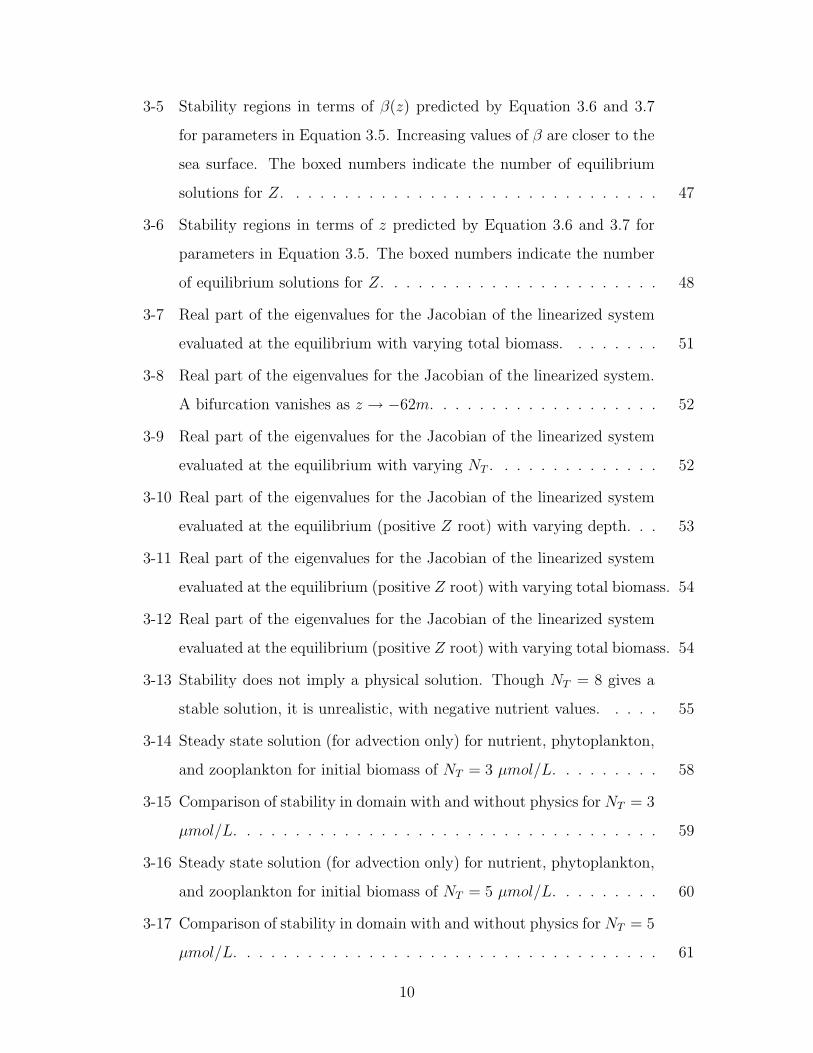
3-5 Stability regions in terms of β(z) predicted by Equation 3.6 and 3.7
for parameters in Equation 3.5. Increasing values of β are closer to the
sea surface. The boxed numbers indicate the number of equilibrium
solutions for Z. . . . . . . . . . . . . . . . . . . . . . . . . . . . . . . 47
3-6 Stability regions in terms of z predicted by Equation 3.6 and 3.7 for
parameters in Equation 3.5. The boxed numbers indicate the number
of equilibrium solutions for Z. . . . . . . . . . . . . . . . . . . . . . . 48
3-7 Real part of the eigenvalues for the Jacobian of the linearized system
evaluated at the equilibrium with varying total biomass. . . . . . . . 51
3-8 Real part of the eigenvalues for the Jacobian of the linearized system.
A bifurcation vanishes as z → −62m. . . . . . . . . . . . . . . . . . . 52
3-9 Real part of the eigenvalues for the Jacobian of the linearized system
evaluated at the equilibrium with varying NT . . . . . . . . . . . . . . 52
3-10 Real part of the eigenvalues for the Jacobian of the linearized system
evaluated at the equilibrium (positive Z root) with varying depth. . . 53
3-11 Real part of the eigenvalues for the Jacobian of the linearized system
evaluated at the equilibrium (positive Z root) with varying total biomass. 54
3-12 Real part of the eigenvalues for the Jacobian of the linearized system
evaluated at the equilibrium (positive Z root) with varying total biomass. 54
3-13 Stability does not imply a physical solution. Though NT = 8 gives a
stable solution, it is unrealistic, with negative nutrient values. . . . . 55
3-14 Steady state solution (for advection only) for nutrient, phytoplankton,
and zooplankton for initial biomass of NT = 3 µmol/L. . . . . . . . . 58
3-15 Comparison of stability in domain with and without physics for NT = 3
µmol/L. . . . . . . . . . . . . . . . . . . . . . . . . . . . . . . . . . . 59
3-16 Steady state solution (for advection only) for nutrient, phytoplankton,
and zooplankton for initial biomass of NT = 5 µmol/L. . . . . . . . . 60
3-17 Comparison of stability in domain with and without physics for NT = 5
µmol/L. . . . . . . . . . . . . . . . . . . . . . . . . . . . . . . . . . . 61
10

3-18 Solution (for advection only) for nutrient, phytoplankton, and zoo-
plankton for initial biomass of NT = 12 µmol/L. . . . . . . . . . . . . 63
3-19 Comparison of stability in domain with and without physics for NT =
12 µmol/L. . . . . . . . . . . . . . . . . . . . . . . . . . . . . . . . . 64
3-20 Steady state solution (for advection and diffusion) for nutrient, phy-
toplankton, and zooplankton for initial biomass of NT = 12 µmol/L.
Diffusion acts to stabilize the previously unstable solution. . . . . . . 65
3-21 Profiles in depth for the steady state solution initialized with NT = 12
µmol/L including diffusion. Unlike the previous case without diffusion,
a steady state was obtainable. Diffusion acts to stabilize the solution. 66
4-1 Initial conditions for nutrients, phytoplankton, and zooplankton. . . . 72
4-2 Arakawa C-grid in the idealized simulation domain with periodic bound-
ary conditions in x and Neumann boundary conditions on the ocean
bottom and air-sea interface. Tracer, horizontal velocity, and verti-
cal velocity nodes are distinguished by circles, squares, and triangles,
respectively. The area under the striped half-ellipse is bathymetry. . . 74
4-3 Placement of Xs in the figure on the right correspond to zeroes in the
mask matrices. A one is placed in the matrix for any node without an
X for the bathymetry shown on the left. . . . . . . . . . . . . . . . . 75
4-4 A one-dimensional view of masking for the example shown in Equa-
tion 4.2. Because we use OSM, this example is representative of our
implemented scheme. The velocity mask is shown on the second line
and the tracer mask is on the third line. . . . . . . . . . . . . . . . . 76
4-5 Initial condition for the one-dimensional test case. . . . . . . . . . . . 79
4-6 Initial condition for the two-dimensional test case. . . . . . . . . . . . 79
4-7 Central difference scheme in two dimensions. Spurious oscillations form
at the bathymetry boundary. . . . . . . . . . . . . . . . . . . . . . . . 80
11
4-8 One-dimensional advection of central difference scheme with a masked
node at x = −17. Oscillations quickly grow and propagate against the
direction of flow. . . . . . . . . . . . . . . . . . . . . . . . . . . . . . 81
4-9 Equation 4.4 is true for interior nodes (i− 1 and i, in this figure). . . 81
4-10 One-dimensional case after three time steps. Because concentration
accumulates at the boundary (i+1) and becomes larger than φi−1, the
finite difference scheme used estimates a decrease in φi at every time
step, so φi becomes more and more negative. . . . . . . . . . . . . . . 82
4-11 Oscillations grow in amplitude and propagate because of their alter-
nating nature. The circular marker indicates the masked node. . . . . 83
4-12 Two-dimensional test case using the donor-cell scheme. There are no
oscillations, but numerical diffusion is present. . . . . . . . . . . . . . 85
4-13 One-dimensional advection of donor-cell scheme with a masked node at
x = −17. Unlike the case using CDS, the concentration accumulated
at the boundary does not produce oscillations. . . . . . . . . . . . . . 85
4-14 Comparison of computational time and numerical diffusion for the
donor-cell scheme (D-C) and central difference scheme. Excluding very
low resolution cases, the central difference scheme has much less diffu-
sion than the donor-cell scheme. Number of nodes used to discretize
the domain is shown for I =15, 50 and 200. . . . . . . . . . . . . . . 87
4-15 Two-dimension test case using γ = 0.5 is absent of oscillations and less
diffusive than the donor-cell scheme. . . . . . . . . . . . . . . . . . . 88
4-16 Hybrid scheme with various values of γ. Even for very small γ, oscil-
latory effects are present. . . . . . . . . . . . . . . . . . . . . . . . . . 89
4-17 Three stencils used in the WENO scheme. . . . . . . . . . . . . . . . 91
4-18 The WENO scheme is not oscillatory and produces a realistic result. . 93
4-19 One-dimensional advection of WENO scheme with a masked node at
x=-17. . . . . . . . . . . . . . . . . . . . . . . . . . . . . . . . . . . . 94
12
4-20 Comparison of computational time versus spread due to numerical dif-
fusion for the donor-cell and WENO schemes. WENO is faster and less
diffusive for higher resolutions. Number of nodes used to discretize the
domain is shown for I =15, 50 and 200. . . . . . . . . . . . . . . . . . 95
4-21 While the modified Thomas Algorithm donor-cell scheme outperforms
the traditional donor-cell scheme, the WENO scheme is better for all
but low resolutions. Diffusion and time are labeled by number of nodes
used to discretize the domain (I =15, 50, 100, 200 and 300). Only
I =300 is shown for the WENO scheme because the other two schemes
have computation times greater than 25 seconds for 300 nodes. . . . . 96
4-22 Streamlines for potential flow over an elliptical bathymetry. . . . . . . 98
4-23 Comparison between simulations using the WENO scheme and Discontinuous-
Galerkin [57]. . . . . . . . . . . . . . . . . . . . . . . . . . . . . . . . 99
5-1 Topography of San Bernardino Strait from Smith and Sandwell. The
dark line is the shortest path through the strait as described in Section
5.1.1. . . . . . . . . . . . . . . . . . . . . . . . . . . . . . . . . . . . . 104
5-2 Bathymetry and initial condition for the two-dimensional simulations
of the San Bernardino Strait. . . . . . . . . . . . . . . . . . . . . . . 105
5-3 Streamlines of the potential flow resulting from the bathymetry of the
San Bernardino Strait. . . . . . . . . . . . . . . . . . . . . . . . . . . 106
5-4 Time scales for the biological reaction terms of Equation 2.3 using
parameters from Equation 3.5. These time scales vary in depth and
with respect to concentration of biological variables. . . . . . . . . . . 109
5-5 Time scales for the biological reaction terms of Equation 2.3 using
region-specific parameters from Table 5.1. This set of parameters leads
to slightly longer time scales than the previous set of parameters. . . 109
5-6 Case 1. No oscillations or diffusion, using parameters in Table 5.1.
Phytoplankton blooms appear because of the vertical velocities caused
by the bathymetry. . . . . . . . . . . . . . . . . . . . . . . . . . . . . 112
13

5-7 Case 2. High frequency oscillations (2 cycles/day), corresponding to
semidiurnal tidal constituents, without diffusion using parameters in
Table 5.1. Increased biological activity seen in Case 1 is not present
and the system has less variation than the similar case without biology
(Figure 5-14). . . . . . . . . . . . . . . . . . . . . . . . . . . . . . . . 113
5-8 Case 3. Low frequency oscillations (1 cycle/day), corresponding to
diurnal tidal constituents, without diffusion using parameters in Table
5.1. Increased biological activity similar to Case 1 is still not present
and the system has less variation than the similar case without biology
(Figure 5-15). . . . . . . . . . . . . . . . . . . . . . . . . . . . . . . . 114
5-9 Case 4. High frequency oscillations (2 cycles/day), corresponding to
semidiurnal tidal constituents, with diffusion using parameters from
Table 5.1 leads to more mixing than Case 2. . . . . . . . . . . . . . . 115
5-10 Case 5. Low frequency oscillations (1 cycle/day), corresponding to
diurnal tidal constituents, with diffusion using parameters from Table
5.1 leads to more mixing than Case 3. . . . . . . . . . . . . . . . . . . 116
5-11 Case 6. High frequency oscillations (2 cycles/day), corresponding to
semidiurnal tidal constituents, without diffusion using parameters match-
ing the three-dimensional case. . . . . . . . . . . . . . . . . . . . . . . 117
5-12 Case 7. Low frequency oscillations (1 cycle/day), corresponding to
diurnal tidal constituents, without diffusion using parameters matching
the three-dimensional case. . . . . . . . . . . . . . . . . . . . . . . . . 118
5-13 Case 8. Very low frequency oscillations (0.1 cycles/day), corresponding
to the longer tidal constituents, without diffusion using parameters
from Table 5.1. Increased biological activity is seen, as tidal period is
similar to the biological time scale. . . . . . . . . . . . . . . . . . . . 119
5-14 Case 9. Non-oscillatory flow without diffusion or biological reaction. . 120
5-15 Case 10. High frequency oscillations (2 cycles/day), corresponding to
semidiurnal tidal constituents, without diffusion or biological reaction. 121
14
5-16 Case 11. Low frequency oscillations (1 cycle/day), corresponding to
diurnal tidal constituents, without diffusion or biological reaction. . . 122
5-17 Case 12. High frequency oscillations (2 cycles/day), corresponding
to longer tidal constituents, without diffusion using parameters from
Table 5.1. This case has double the velocity of previous cases. . . . . 123
5-18 Regions of the Philippine Archipelago with different chlorophyll pro-
files. Dark blue represents the South China Sea, yellow is the Sulu Sea,
cyan is the Pacific, and red represents the interior seas. . . . . . . . . 125
5-19 Example of generic profiles for chlorophyll were scaled according to
the surface integrated chlorophyll value from satellite images. xs dis-
tinguish peaks from the background value. . . . . . . . . . . . . . . . 126
5-20 Objectively analyzed chlorophyll field from the PhilEx IOP09 cruise
data using the Fast Marching Method. The scales used in the OA
are: synoptic decay–90km, mean decay–360km, synoptic zero crossing–
270km, mean zero crossing–1080km. . . . . . . . . . . . . . . . . . . . 127
5-21 Results from MSEAS for the San Bernardino Strait. . . . . . . . . . . 130
A-1 ρ, s, and ρ2 for NT = 2 µmol/L over entire depth range β. Transitions
only occur for very small β (deep water), shown in Figure A-2. . . . . 138
A-2 At β = 0, ρ < 0 and s > 0, so no solutions are present. After approxi-
mately β = 0.01, s < 0 and one solution appears. At about β = 0.0275,
ρ > 0 and only one solution is still present. This corresponds to NT = 2
µmol/L, which is the second row of Table A.1. . . . . . . . . . . . . . 139
A-3 ρ, s, and ρ2 forNT = 2.2 µmol/L over entire depth range β. Transitions
only occur for very small β (deep water), shown in Figure A-4. . . . . 139
A-4 For all β, s < 0. For β < 0.01, ρ < 0 (one solution) and for β > 0.01,
ρ > 0 (again, one solution). This corresponds to NT = 2.2 µmol/L,
which is the third row of Table A.1. . . . . . . . . . . . . . . . . . . . 140
A-5 ρ, s, and ρ2 for NT = 3 µmol/L over entire depth range β. Transitions
only occur for very small β (deep water), shown in Figure A-6. . . . . 140
15
A-6 For all β, ρ > 0. For β < 0.02, s < 0 (one solution) and for β > 0.02,
s > 0 (two solutions). This corresponds to NT = 3 µmol/L, which is
the last row of Table A.1. . . . . . . . . . . . . . . . . . . . . . . . . 141
A-7 Zooplankton equilibrium for various NT values with the solid line repre-
senting the positive root of zooplankton and the dashed line represent-
ing the negative root. The number of physical solutions corresponds
to the predictions made in the previous figures. For NT = 2 µmol/L,
we see that for very small β, there are no solutions, then the posi-
tive root becomes a physical solution for all β above a critical value.
For NT = 2.2 µmol/L, we always have one solution and for NT = 3
µmol/L, we have one solution for small β, then two solutions as β grows.141
A-8 Nutrient equilibrium for various NT values with the solid line repre-
senting the positive root of nutrient and the dashed line representing
the negative root. The number of physical solutions corresponds to the
predications made in the previous figures. For NT = 2 µmol/L, we see
that for very small β, there are no solutions, then the negative root be-
comes a physical solution for all β above a critical value. For NT = 2.2
µmol/L, we always have one solution and for NT = 3 µmol/L, we have
one solution all β. . . . . . . . . . . . . . . . . . . . . . . . . . . . . . 142
16
List of Tables
2.1 Descriptions of generic biological reaction terms . . . . . . . . . . . . 30
3.1 Number of zooplankton equilibrium points with ρ, s, and β(z). βcs is
the depth where s changes sign and βcρ is the depth where ρ changes
sign. . . . . . . . . . . . . . . . . . . . . . . . . . . . . . . . . . . . . 45
3.2 Number of zooplankton equilibrium based on total biomass (NT ), depth,
and the sign of ρ and s. βc1 and βc2 are chosen based on the values of
βcρ and βcs. For instance, if βcρ > βcs, then βc1 = βcs and βc2 = βcρ. . 46
3.3 Critical values for parameter values listed in Equation 3.5, also pre-
sented in Figure 3-5. . . . . . . . . . . . . . . . . . . . . . . . . . . . 46
3.4 Stability regions (in total biomass, limited by z = 0) for parameter
values listed in Equation 3.5. . . . . . . . . . . . . . . . . . . . . . . . 55
3.5 Stability region limits, defined by parameters. Starred values must be
solve numerically because those parameters are included in γ. . . . . 56
3.6 Results of the phase portraits in Appendix B. . . . . . . . . . . . . . 57
5.1 Region specific parameters for the Philippine Archipelago. . . . . . . 102
5.2 Two-dimensional cases examined using the idealized numerical simula-
tion. Varying frequencies, parameters and levels of diffusion are studied.108
5.3 Parameters used in the four-dimensional biological-physical simula-
tions for the PhilEx real-time IOP09 experiment. . . . . . . . . . . . 128
17

A.1 Number of zooplankton equilibrium based on total biomass (NT ), depth,
and the sign of ρ and s. Figures included in this Appendix show that
ρ and s can be plotted easily to determine the number of solutions for
a given depth. . . . . . . . . . . . . . . . . . . . . . . . . . . . . . . . 138
B.1 Predicted stability of the phase portraits for P versus Z. . . . . . . . 143
18
Chapter 1
Introduction
1.1 Motivation and Background
Ocean straits and archipelagos create complex physical domains, resulting in pro-
cesses spanning many time and spatial scales. These conditions lead to interesting
biological phenomena, including diverse blooms of biota. Identifying which processes
and conditions are necessary and sufficient for such blooms to occur is a challenging
task, especially in domains as complicated as archipelagos. By isolating processes,
we can improve our understanding of the relationship between physical processes
and biology. We conduct research toward understanding coupled physics-biology pro-
cesses in ocean straits through new analytical studies and higher-order simulations
of idealized dynamics that are relevant to generic biology in straits. Specifically,
we first characterize global equilibrium properties and the local stability of biologi-
cal reaction equations in a non-diffusive framework without flow. We then develop
and utilize a new higher-order numerical scheme for two-dimensional simulations of
coupled physical-biological dynamics over straits, with a focus on tidal effects. We
study tidal effects because they often strongly determine flow in straits at diurnal
and semidiurnal periods, but their oscillations may be too fast for certain biological
reactions.
Our research efforts are a part of the Philippines Experiment, or PhilEx, a five-
year joint research project focused on interdisciplinary modeling, data assimilation
19

and dynamical studies in the straits regions of the Philippine Archipelago to bet-
ter understand, model and predict sub-mesoscale and mesoscale physical and bio-
geochemical dynamics in sea straits. The three-dimensional ocean model fields and
measurements from PhilEx are used in this study. Gathering biological data is fre-
quently done by capturing water samples, using underwater vehicles, or instruments
attached to a research vessel, which leads to sparse data fields in space and time.
Previous research and data is scarce in the Philippines, therefore initializing models
is challenging. We thus develop a new method to initialize coupled physics-biology
with sparse initial data.
The Philippines region has very interesting dynamics including a wide range of
physical processes, a seasonal monsoon, and transport through straits from various
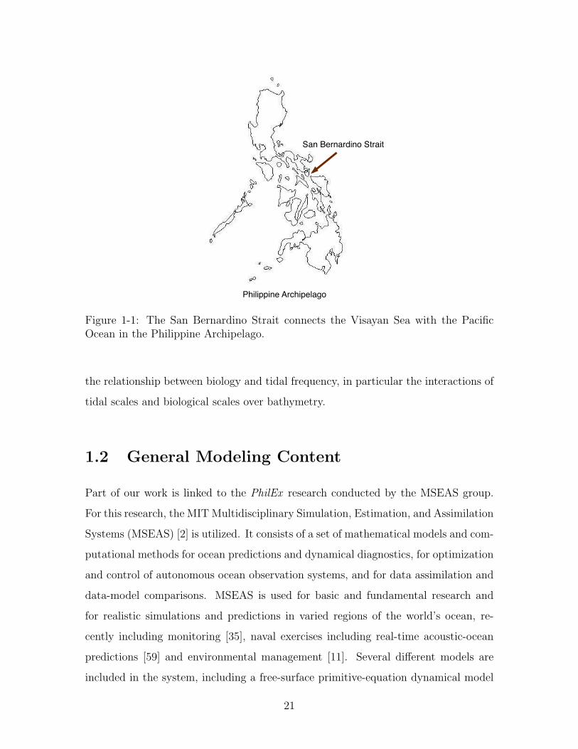
ocean basins. The San Bernardino Strait in the Philippines connects the Visayan Sea
with the Pacific Ocean. Experimental data suggests that the San Bernardino Strait
hinders flow of intermediate and deep waters from entering the archipelago [41]. Tides
in this region reduce the mean flow through the strait by nonlinear rectification [27],
which causes considerable phase and amplitude shifts [37]. Both topography and
intense tidal mixing are strongly influential in this strait [27]. Thus, the topography
and flow from the San Bernardino Strait in the Philippine Archipelago is used to
create realistic test cases. The location of the San Bernardino Strait within the
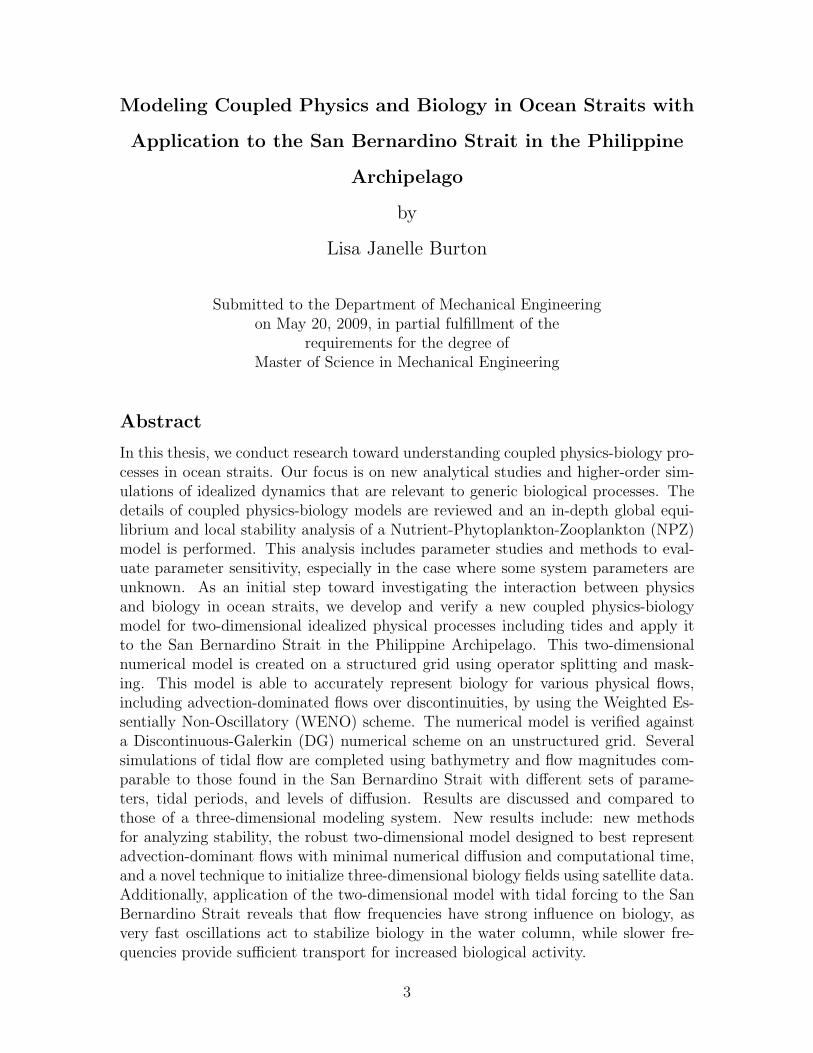
Philippine Archipelago is shown in Figure 1-1.
Previous research on the topic of tides and biology shows that tidal mixing pro-
duces increased biomass. This research has been performed both experimentally and
theoretically, though it is difficult to sample biology fine enough to resolve some of
the features predicted. Tidal effects on biology have been primarily explored in the
open ocean [5], [19], fjords [31], banks [21] and estuaries [50]. These studies examine
the source of dense biomass concentrations due to tidal pumping and forcing. Aside
from straits with both historical data and thorough understanding of the tidal effects,
such as the Strait of Gibraltar [39], no research has been conducted, to the author’s
knowledge, on the topic of general biology in ocean straits including coupled biology-
tidal effects. The work completed in this thesis is an initial step to understanding
20
San Bernardino Strait
Philippine Archipelago
Figure 1-1: The San Bernardino Strait connects the Visayan Sea with the PacificOcean in the Philippine Archipelago.
the relationship between biology and tidal frequency, in particular the interactions of
tidal scales and biological scales over bathymetry.
1.2 General Modeling Content
Part of our work is linked to the PhilEx research conducted by the MSEAS group.
For this research, the MIT Multidisciplinary Simulation, Estimation, and Assimilation
Systems (MSEAS) [2] is utilized. It consists of a set of mathematical models and com-
putational methods for ocean predictions and dynamical diagnostics, for optimization
and control of autonomous ocean observation systems, and for data assimilation and
data-model comparisons. MSEAS is used for basic and fundamental research and
for realistic simulations and predictions in varied regions of the world’s ocean, re-
cently including monitoring [35], naval exercises including real-time acoustic-ocean
predictions [59] and environmental management [11]. Several different models are
included in the system, including a free-surface primitive-equation dynamical model
21
which uses two-way nesting free-surface and open boundary condition schemes [26].
This new free-surface code is based on the primitive-equation model of the Harvard
Ocean Prediction System (HOPS). Additionally, barotropic tides are calculated from
the inverse tidal model [38].
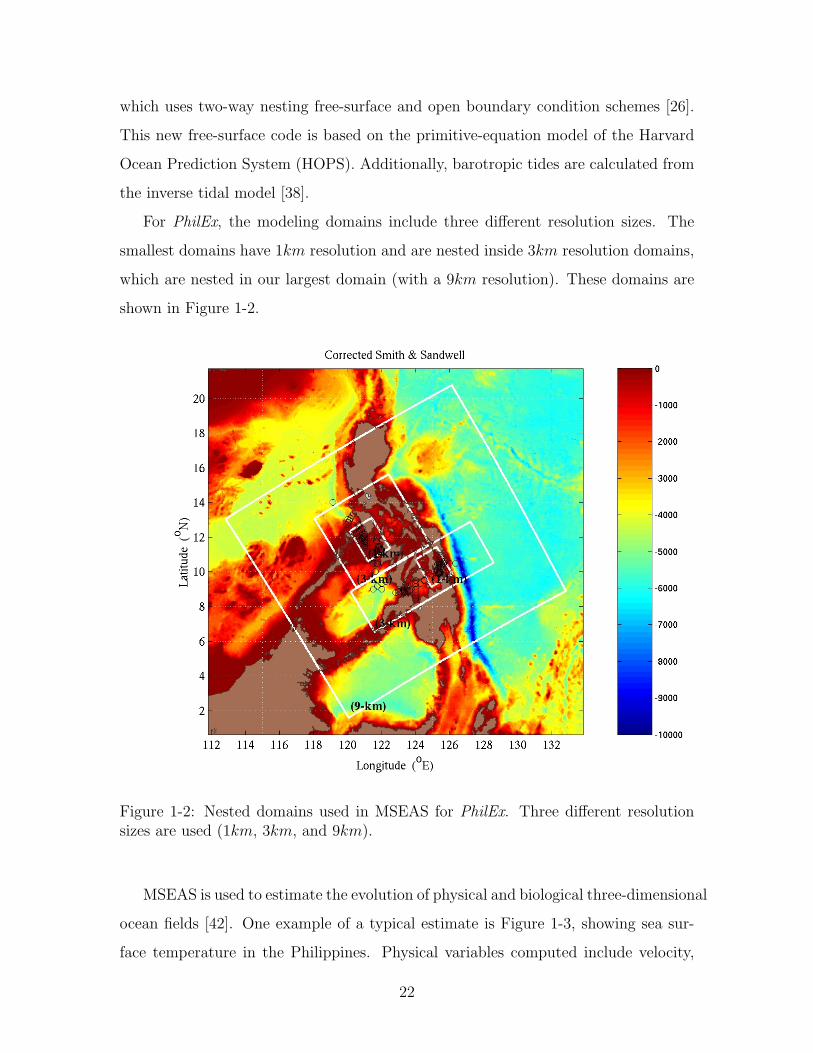
For PhilEx, the modeling domains include three different resolution sizes. The
smallest domains have 1km resolution and are nested inside 3km resolution domains,
which are nested in our largest domain (with a 9km resolution). These domains are
shown in Figure 1-2.
Figure 1-2: Nested domains used in MSEAS for PhilEx. Three different resolutionsizes are used (1km, 3km, and 9km).
MSEAS is used to estimate the evolution of physical and biological three-dimensional
ocean fields [42]. One example of a typical estimate is Figure 1-3, showing sea sur-
face temperature in the Philippines. Physical variables computed include velocity,
22

temperature and salinity. Biological variables depend on the biological model used.
1.3 Thesis Overview
In Chapter 2, we discuss physical and biological models. For the biology, Nutrient-
Phytoplankton-Zooplankton (NPZ) models (for a two-dimensional simulation) and
more complex biogeochemical models (for a three-dimensional simulation) are dis-
cussed. To determine parameter limitations and sensitivity, we perform new global
equilibrium and local stability analyses in Chapter 3 of the biological reaction equa-
tions in a non-diffusive, conservative framework without physics. General analytical
methods to determine equilibria and stability properties for a parameter set are de-
veloped and demonstrated. Conditions necessary for stability and instability are dis-
cussed and application to the domain including advection and diffusion is presented.
To study idealized coupled physical and biological dynamics accurately, we implement
and compare various numerical schemes in Chapter 4 to identify high-order schemes
with low numerical diffusion able to represent a wide range of processes, including
the advection dominant case (which is prone to oscillations). All details of the de-
velopment of the simulation are outlined and the result is a new scheme resistant
to oscillations with easy implementation of boundary conditions and low numerical
diffusivity. In Chapter 5, we use this numerical scheme to study the effects of tides in
a two-dimensional strait-like domain, varying biological parameters, tidal frequency,
and levels of diffusion. We then present our new approaches for the initialization of
a three-dimensional biological model in MSEAS using sparse data which is based on
region-specific analytic chlorophyll profiles. The biology fields are compared to the
two-dimensional fields. All results are reviewed and summarized in Chapter 6.
23

Figure 1-3: An example output from MSEAS showing surface temperature and cur-rent for the archipelago domain. Cross-sectional plots are also produced along selectstraits [43].
24
Chapter 2
Modeling Physics and Biology
In this chapter, we discuss details of coupled physics-biological modeling. Models of
varying levels of complexity are explored and two models are selected for analysis
in subsequent chapters. The first model described is a simplified NPZ (Nutrient-
Phytoplankton-Zooplankton) model for an idealized system in two spatial dimensions.
This model allows closed form analytic results that reveal important characteristics
of the system and allow parameter sensitivity studies. The second model described
is significantly more complex, including additional biological and chemical variables.
This later model is sufficiently sophisticated to provide accuracy and precision re-
quired for three dimensional modeling using MSEAS. We show that these models are
appropriate tools to use for an initial assessment of the relationship between physics
and biology. Various ways to represent biological processes are compared and dis-
cussed.
2.1 Biology in the Ocean
Unlike most physical systems, equations to model biological systems in the ocean
have not yet been derived from first principles and conservation laws. Instead, the
governing equations for biological systems are built from observations. These em-
pirical equations often contain several region-specific parameters to describe growth
rates, death rates, and other processes [16]. While the equations model how the state
25

variables interact, the parameters control the characteristics of interaction, including
the rates of growth or death.
To study the relationship between physics and biology, it is common to examine
the lower trophic levels of biology. Modeling is often limited to an isolated part of
the food web, such as the cycle between nutrients, phytoplankton, and zooplankton.
Phytoplankton feed on nutrients and are consumed by zooplankton. When zooplank-
ton die, bacteria eventually convert the zooplankton back to nutrients. The growth
rate of each of these organisms is dependent on the environment and the specific
quantities of the other organisms. As such, the relationship between the different
organisms is highly coupled. The presence or absence of one organism determines the
growth possible by another.
The relationships which represent biological interaction between organisms, called
reaction or source terms, can be expressed in various ways and depend on several
parameters. These parameters, discussed in Section 2.2, can be a function of space
and time and are region-dependent. Sufficient data is needed to specify temporal and
spatial variation of parameters. Temporal variations include seasonal, weekly, or daily
scales and examples of spatial variations include varying parameters from one region
to another, or in depth. For the present research, we are interested in parameters
appropriate for the Philippines but we will start with constant parameters because
of sparse data in this region.
Environmental factors important to biological growth include light (solar irra-
diance), bottom depth, availability of nutrients and physical processes such as tur-
bulence, internal waves, and eddy transport [17]. These factors can directly affect
single or multiple state variables. (A biological state variable is usually the biomass
concentration of an organism such as zooplankton, phytoplankton, and nutrients.)
For instance, only phytoplankton require light. They must live near the ocean sur-
face to absorb light for photosynthesis. Experiments in some regions have shown
that phytoplankton growth can be hindered by too little or too much light. Because
phytoplankton require light, there exists a critical depth where insufficient sunlight
eliminates the possibility of phytoplankton (and thus zooplankton) growth, assuming
26

a domain without flow. Critical depth is defined as the depth where photosynthetic
gain of phytoplankton cells are balanced by respiratory losses, which can be different
than the depth of the euphotic zone, where light is sufficient to support plant growth
[33].
If flow, such as a downward vertical velocity or diffusion, is present, phytoplankton
may be transported from above the critical depth down to light-deficient areas, in
which case the depth of the euphotic zone and the critical depth do not coincide.
These depths vary highly with location, depending on the local turbidity of the water
and the attenuation of light with depth. In Chapter 3, we discuss the validity of
critical stability depth (found in the reference frame without physics) when advection
and diffusion are present. In general, in open ocean conditions, the greatest local
variation in biomass is in vertical distribution because of light-dependence and ocean
flows, which are commonly much stronger in the horizontal direction than in the
vertical.
Only some species of plankton are capable of independent vertical movement. Ex-
cluding these, plankton and nutrients act as passive tracers in the flow because their
self-movement in comparison to the flow is negligible [18]. Therefore biology, which
act as passive tracers, can be good indicators of flow direction and strength. Physical
processes that increase vertical velocities and mixing often produce interesting biolog-
ical behaviors. We will model physical processes by considering advection (transport
by ocean currents) and diffusion (mixing processes) [17]. When nutrient-rich waters
are upwelled, a more productive environment is created because phytoplankton gain
access to these nutrients. Predicting and understanding processes such as upwelling
is key in understanding how changing conditions will affect marine life, an important
food source to the world. Currently, regions of coastal upwelling are responsible for
approximately half of the fish harvest in the world, though they only occupy 0.1%
of the ocean’s surface area [12]. Further, advection and diffusion can raise or lower
the critical depth (compared to the critical depth of the physics-free reference frame).
Consider an extreme case with very high diffusion. High rates of mixing create an
averaged field, so that the concentration of phytoplankton at the surface matches
27

the value at the ocean floor. Therefore, no critical depth exists and phytoplankton
growing at one depth are transported quickly to the entire water column.
Although we are only considering lower trophic levels in our models, the behavior
and trends are indicative of higher trophic levels. The relationship between the two is
sometimes extremely short. For example, whales consume krill (a type of zooplank-
ton), which consume phytoplankton. All higher trophic level activity depends on
these primary producers. In general, we assume zooplankton are consumed by fish,
which are either caught by man or eventually recycled into nutrients [16].
2.2 Two-dimensional Idealized Case: Nutrient-
Phytoplankton-Zooplankton Model
There are several types of biological ocean models ([49], [30]). We focus on the NPZ
(Nutrient-Phytoplankton-Zooplankton) food-web model for our idealized simulation.
It is a concentration-based model, with nitrogen or carbon as a currency. An NPZ
model is chosen because it is one of the most basic ways to represent the biological-
physical interactions for lower trophic levels [20]. NPZ models accurately represent
a wide range of biological behaviors, as evidenced by many example of successful
usage, both quantitatively and qualitatively. NPZ models are not commonly used for
predictive purposes, but are useful in understanding past trends and behaviors. NPZ
models are appropriate for mesoscale physical processes because of matching time
scales with biological interactions.
The NPZ model preserves first order interactions, but is simplified enough to per-
mit analytic, closed form results with or without numeric methods. An NPZ model
assumes that zooplankton feed on phytoplankton, which feed on nutrients. Zooplank-
ton and phytoplankton each have a natural mortality rate. When zooplankton and
phytoplankton die naturally, we assume that they directly become nutrients. Fig-
ure 2-1 shows a graphical representation of the NPZ model just described. Other
food-web models that include additional compartments and complexities are used in
28
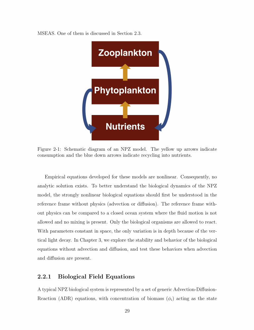
MSEAS. One of them is discussed in Section 2.3.
Zooplankton
Phytoplankton
Nutrients
Figure 2-1: Schematic diagram of an NPZ model. The yellow up arrows indicateconsumption and the blue down arrows indicate recycling into nutrients.
Empirical equations developed for these models are nonlinear. Consequently, no
analytic solution exists. To better understand the biological dynamics of the NPZ
model, the strongly nonlinear biological equations should first be understood in the
reference frame without physics (advection or diffusion). The reference frame with-
out physics can be compared to a closed ocean system where the fluid motion is not
allowed and no mixing is present. Only the biological organisms are allowed to react.
With parameters constant in space, the only variation is in depth because of the ver-
tical light decay. In Chapter 3, we explore the stability and behavior of the biological
equations without advection and diffusion, and test these behaviors when advection
and diffusion are present.
2.2.1 Biological Field Equations
A typical NPZ biological system is represented by a set of generic Advection-Diffusion-
Reaction (ADR) equations, with concentration of biomass (φi) acting as the state
29

Reaction term Representation Description
uptake(P,N) f(I)g(N) Phytoplankton response to irradiance &Phytoplankton nutrient uptake
grazing(P,Z) h(P ) Zooplankton grazing on phytoplanktondeath(P) i(P ) Phytoplankton death ratedeath(Z) j(Z) Zooplankton death rateregeneration(P,Z) (1− α)h(P ) Inefficiency of zooplankton grazingassimilation(P,Z) αh(P ) Efficiency of zooplankton grazing
Table 2.1: Descriptions of generic biological reaction terms
variable. The second term of Equation 2.1 is advection, the third diffusion, and the
last term represents the collection of biological reaction terms.
∂φi∂t
+∇ · (uφi) = ∇ · κ∇φi + B(φ1, ..., φi, ..., φN) (2.1)
where (φ1...φN) are the N state variables, κ is the diffusion coefficient, and u is the
velocity vector. These equations are also valid for the more complex model described
in Section 2.3.
B(φ1, φ2, ..., φN) couples the equations for different organisms.
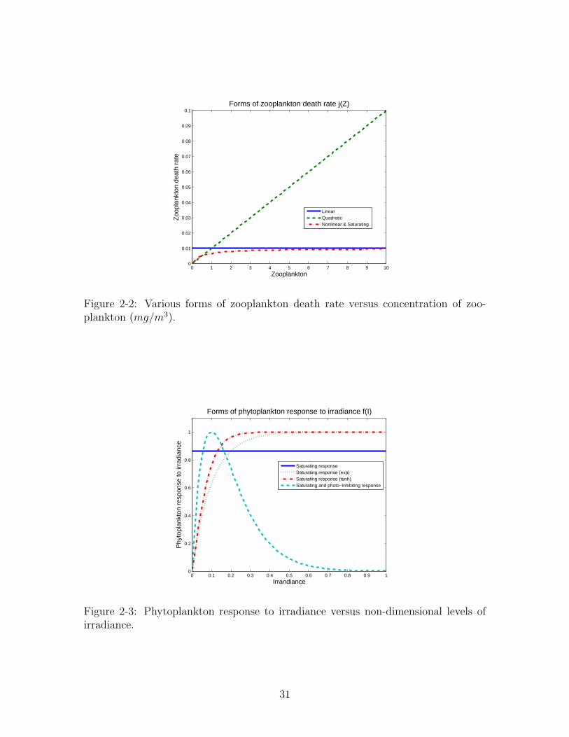
Biological reactions typically modeled in NPZ equations are described by [18]
and [20] and summarized in Table 2.1. The reaction terms listed in the table can
take many forms, depending on the relationship modeled. For instance, to model
zooplankton death rate (j(Z)) and the phytoplankton response to irradiance (f(I))
several different relationships can be used and are shown in Figures 2-2 and 2-3. The
curves in Figure 2-2 present reaction terms for zooplankton death rate for various
level of complexity. It is clear that the nonlinear term models the same behavior of
quadratic death rate for low concentrations of zooplankton and matches linear death
rate for high concentrations of zooplankton, with a smooth transition in between for
mid-range concentrations. Figure 2-3 demonstrates the response of phytoplankton to
irradiance. Again, we see that adding complexity allows behavior at both low and
high irradiance to be specified. The last curve (according to the legend) models a
response for phytoplankton, which is sensitive to both too little and too much light.
30
0 1 2 3 4 5 6 7 8 9 100
0.01
0.02
0.03
0.04
0.05
0.06
0.07
0.08
0.09
0.1
Zoo
plan
kton
dea
th r
ate
Zooplankton
Forms of zooplankton death rate j(Z)
LinearQuadraticNonlinear & Saturating
Figure 2-2: Various forms of zooplankton death rate versus concentration of zoo-plankton (mg/m3).
0 0.1 0.2 0.3 0.4 0.5 0.6 0.7 0.8 0.9 10
0.2
0.4
0.6
0.8
1
Phy
topl
ankt
on r
espo
nse
to ir
radi
ance
Irrandiance
Forms of phytoplankton response to irradiance f(I)
Saturating responseSaturating response (exp)Saturating response (tanh)Saturating and photo−inhibiting response
Figure 2-3: Phytoplankton response to irradiance versus non-dimensional levels ofirradiance.
31
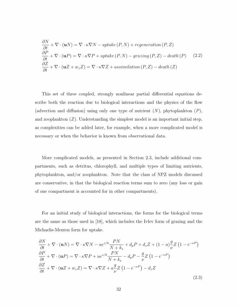
∂N
∂t+∇ · (uN) = ∇ · κ∇N − uptake (P,N) + regeneration (P,Z)
∂P
∂t+∇ · (uP ) = ∇ · κ∇P + uptake (P,N)− grazing (P,Z)− death (P )
∂Z
∂t+∇ · (uZ + wzZ) = ∇ · κ∇Z + assimilation (P,Z)− death (Z)
(2.2)
This set of three coupled, strongly nonlinear partial differential equations de-
scribe both the reaction due to biological interactions and the physics of the flow
(advection and diffusion) using only one type of nutrient (N ), phytoplankton (P),
and zooplankton (Z ). Understanding the simplest model is an important initial step,
as complexities can be added later, for example, when a more complicated model is
necessary or when the behavior is known from observational data.
More complicated models, as presented in Section 2.3, include additional com-
partments, such as detritus, chlorophyll, and multiple types of limiting nutrients,
phytoplankton, and/or zooplankton. Note that the class of NPZ models discussed
are conservative, in that the biological reaction terms sum to zero (any loss or gain
of one compartment is accounted for in other compartments).
For an initial study of biological interactions, the forms for the biological terms
are the same as those used in [18], which includes the Ivlev form of grazing and the
Michaelis-Menten form for uptake.
∂N
∂t+∇ · (uN) = ∇ · κ∇N − uez/h PN
N + ks+ dpP + dzZ + (1− a)
g
νZ(1− e−νP
)∂P
∂t+∇ · (uP ) = ∇ · κ∇P + uez/h
PN
N + ks− dpP −
g
νZ(1− e−νP
)∂Z
∂t+∇ · (uZ + wzZ) = ∇ · κ∇Z + a
g
νZ(1− e−νP
)− dzZ
(2.3)
32
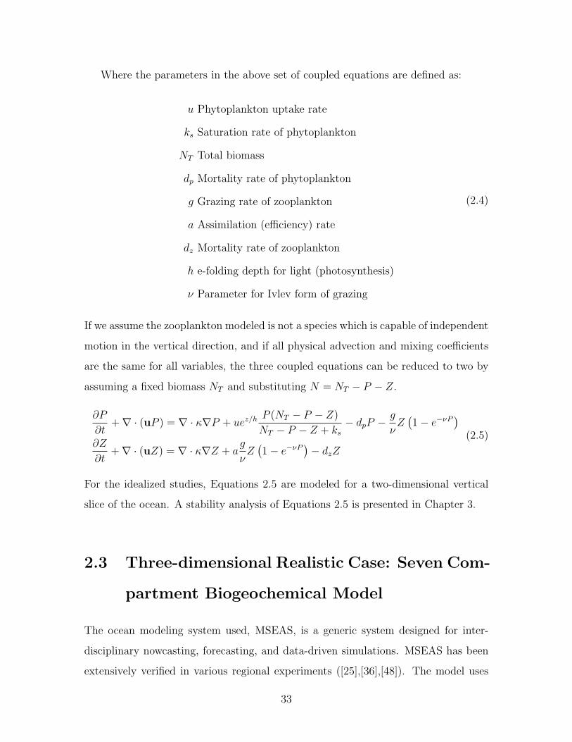
Where the parameters in the above set of coupled equations are defined as:
u Phytoplankton uptake rate
ks Saturation rate of phytoplankton
NT Total biomass
dp Mortality rate of phytoplankton
g Grazing rate of zooplankton
a Assimilation (efficiency) rate
dz Mortality rate of zooplankton
h e-folding depth for light (photosynthesis)
ν Parameter for Ivlev form of grazing
(2.4)
If we assume the zooplankton modeled is not a species which is capable of independent
motion in the vertical direction, and if all physical advection and mixing coefficients
are the same for all variables, the three coupled equations can be reduced to two by
assuming a fixed biomass NT and substituting N = NT − P − Z.
∂P
∂t+∇ · (uP ) = ∇ · κ∇P + uez/h
P (NT − P − Z)
NT − P − Z + ks− dpP −
g
νZ(1− e−νP
)∂Z
∂t+∇ · (uZ) = ∇ · κ∇Z + a
g
νZ(1− e−νP
)− dzZ
(2.5)
For the idealized studies, Equations 2.5 are modeled for a two-dimensional vertical
slice of the ocean. A stability analysis of Equations 2.5 is presented in Chapter 3.
2.3 Three-dimensional Realistic Case: Seven Com-
partment Biogeochemical Model
The ocean modeling system used, MSEAS, is a generic system designed for inter-
disciplinary nowcasting, forecasting, and data-driven simulations. MSEAS has been
extensively verified in various regional experiments ([25],[36],[48]). The model uses
33
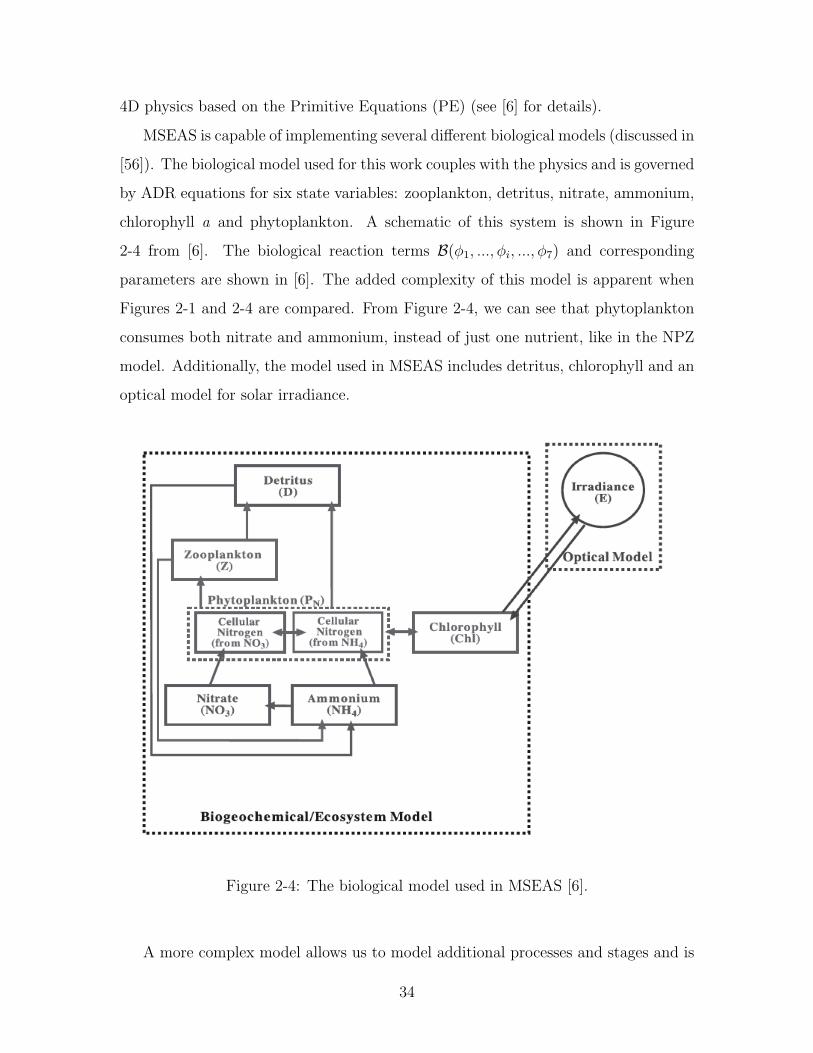
4D physics based on the Primitive Equations (PE) (see [6] for details).
MSEAS is capable of implementing several different biological models (discussed in
[56]). The biological model used for this work couples with the physics and is governed
by ADR equations for six state variables: zooplankton, detritus, nitrate, ammonium,
chlorophyll a and phytoplankton. A schematic of this system is shown in Figure
2-4 from [6]. The biological reaction terms B(φ1, ..., φi, ..., φ7) and corresponding
parameters are shown in [6]. The added complexity of this model is apparent when
Figures 2-1 and 2-4 are compared. From Figure 2-4, we can see that phytoplankton
consumes both nitrate and ammonium, instead of just one nutrient, like in the NPZ
model. Additionally, the model used in MSEAS includes detritus, chlorophyll and an
optical model for solar irradiance.
Figure 2-4: The biological model used in MSEAS [6].
A more complex model allows us to model additional processes and stages and is
34
often more realistic. However, it presents the challenge of initializing the system (now
in three spatial dimensions and for six state variables, compared to two dimensions
with three variables as in the NPZ model), and additional difficulty in understanding
the strongly nonlinear coupled equations. While we were able to simplify Equation
2.3 to Equations 2.5, no such simplification is possible for the MSEAS model. Initial-
ization of the system depends on the data available in the region of interest. Details
on the initialization of the biological system for the Philippines domain are discussed
in Chapter 5.
Both models chosen for analysis and simulation of coupled physics and biology
have been previously tested and verified. Each has its advantages: the NPZ model
offers the ability to obtain closed form solutions describing the system, while the
model used in MSEAS is capable of modeling more complex, realistic behaviors.
These models are thus appropriate tools to use for understanding the relationship
between coupled physics and biology in the Philippine Archipelago, a region where
relatively little data is available. However, after more information is known about
the region, we may find it suitable to use different reaction terms or a different model
that is more fitting.
35

36
Chapter 3
Stability and Equilibria of the
Nutrient-Phytoplankton-
Zooplankton Model
Understanding the detailed relationships between the state variables of Equation 2.3
solely by examining terms is very challenging. The biological reaction terms are
strongly nonlinear and depend on parameters that may take different values for dif-
ferent regions. It is common to use coupled biological-physical models in regions
where not all of the parameters are known. In this case, it is important to know
which range of parameter values give physical solutions and which cause unstable
or unrealistic solutions. Additionally, if parameters are estimated (either because
they are unknown or because several different values have been recorded for a re-
gion), knowing how sensitive the equations are to a particular parameter indicates
the necessary level of accuracy for the parameter estimates.
In this chapter, we consider the reference frame without physics (that is, advec-
tion or diffusion) to express important equilibrium and global stability properties in
an analytic, closed form fashion, purely in terms of the system parameters. While
numerical models are very powerful tools in simulating coupled physics and biology,
an analytic stability analysis allows us to learn a substantial amount of global in-
formation quickly and easily by evaluating first-order dependencies and relationships
37
between parameters, stability, and equilibria. These results are particularly useful
if some of the parameters are known so that there are fewer degrees of freedom to
analyze. The use of Direct Numerical Simulation to obtain comparable global results
would require significant time and effort to tune parameters and analyze test cases.
More specifically, Section 3.1 presents a novel global stability analysis of the bio-
logical equations (without advection or diffusion) conducted to evaluate the sensitiv-
ity of the strongly nonlinear equations to parameter values, behavior of the equilibria
states, as well as appropriate ranges for the parameter values. In Section 3.2, we focus
more on local stability, studying critical stability depths and presenting a new gen-
eral method of stability analysis showing results for varying total amount of biomass
concentration in the system (NT ). Lastly, the applicability of the stability analysis
in the dynamics model (including physics) is addressed.
3.1 Equilibria Solutions and Regions
To obtain static equilibria solutions, we consider Equations 2.5 without advection or
diffusion:
dP
dt= uez/h
P (NT − P − Z)
NT − P − Z + ks− dpP −
g
νZ(1− e−νP
)dZ
dt= a
g
νZ(1− e−νP
)− dzZ
(3.1)
Note that these equations are identical to the biological equation in the Lagrangian
frame, including advection, where ddt
is the material derivative. Equations 3.1 are set
to zero to solve for the steady equilibria. Once the system is in steady state, it does
not change with time, so we set the time derivative to zero to solve for P and Z in
this state. As mentioned in Chapter 2, we have constant total biomass NT in the
system if we assume there is no independent swimming zooplankton, so our nutrient
equation is simply N = NT − P − Z. These equations essentially represent how
phytoplankton and zooplankton change in time due to the biological reaction terms
38

only. For biological modeling in a region with sufficient information, NT may be
modeled as varying in space (more commonly in depth only) or in time. In that case,
the following analysis is appropriate for any point in time with constant biomass.
Commonly, NT is modeled as constant in space and time, in which case the analysis
is valid in the entire field.
The steady state equations (Equations 3.1) give three sets of equilibria (Equations
3.2-3.4). The first equilibrium is:
N = NT
P = 0
Z = 0
(3.2)
Equations 3.2 are the solutions we expect in deep waters where phytoplankton are
unable to survive, thus zooplankton have nothing to feed on. Therefore, nutrients are
responsible for the full biomass value. The second equilibrium is:
N = −ks −β(z)ksdp − β(z)
P = ks +NT +β(z)ksdp − β(z)
Z = 0
(3.3)
Equations 3.3 will always give negative amounts of biomass, an unphysical solution,
and thus we are not interested in these steady state values. The third equilibrium is:
N = NT +γ
ν− ρ∓
√ρ2 − s
P = −γν
Z = ρ±√ρ2 − s
(3.4)
39
where
ρ =1
2
(ks +NT +
γ
ν
(1 +
a
dz(dp − β(z))
))s =
aγ
dzν
(dp
(γν
+NT + ks
)− β(z)
(γν
+NT
))γ = ln
(1− dzν
ag
)β(z) = uez/h
It is important to note that γ ≤ 0 and 0 ≤ β(z) ≤ u because all parameters in
Equation 3.1 are positive. Further, β(z) can be thought of as a generalized depth
that does not require specification of e-folding depth h (describing how light decays
in depth) or uptake rate u. For near surface depths, limz→0 β(z) = u while for depths
far below the surface, limz→−∞ β(z) = 0.
Equations 3.4 are the most interesting because they represent the physically re-
alistic biological equilibrium in the upper layer of the ocean. Altering the system
parameters can change the equilibrium from positive to negative and real to imagi-
nary. Knowing that γ is always non-positive and ν is always positive guarantees a
positive value of phytoplankton equilibria. Phytoplankton equilibria is independent
of depth z or β(z), so this result is valid (positive and real) for the entire water
column above the critical depth. Below the critical depth, phytoplankton cannot sur-
vive and nutrients dominate. More technically, the critical depth is the depth where
photosynthetic gain of phytoplankton cells are balanced by respiratory losses [33].
Because of mixing, the critical depth does not necessarily correspond to the depth of
the euphotic zone, where light is sufficient to support plant growth.
For initial analysis, we will use the parameter values used in [18] to study the
behavior of the last set of equilibria. These values are:
40
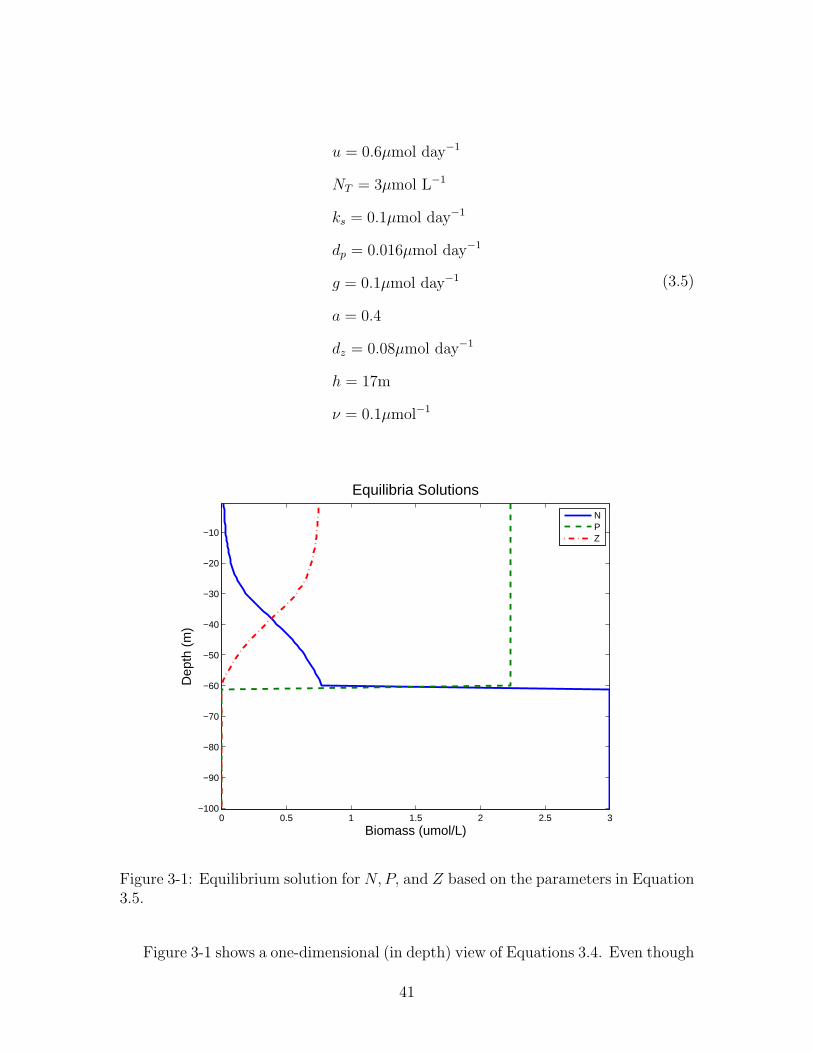
u = 0.6µmol day−1
NT = 3µmol L−1
ks = 0.1µmol day−1
dp = 0.016µmol day−1
g = 0.1µmol day−1
a = 0.4
dz = 0.08µmol day−1
h = 17m
ν = 0.1µmol−1
(3.5)
0 0.5 1 1.5 2 2.5 3−100
−90
−80
−70
−60
−50
−40
−30
−20
−10
Biomass (umol/L)
Dep
th (
m)
Equilibria Solutions
NPZ
Figure 3-1: Equilibrium solution for N,P, and Z based on the parameters in Equation3.5.
Figure 3-1 shows a one-dimensional (in depth) view of Equations 3.4. Even though
41
phytoplankton feeding decays in depth because they require light for photosynthesis,
the phytoplankton equilibria do not vary with depth, until the solutions become
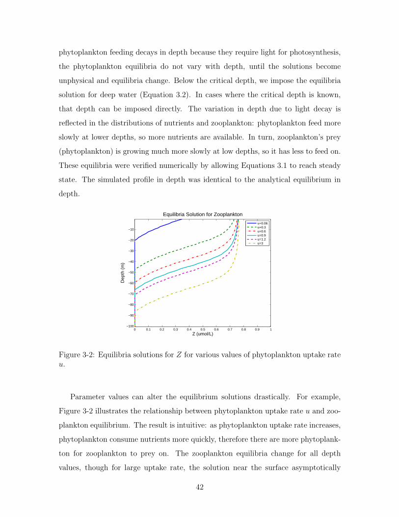
unphysical and equilibria change. Below the critical depth, we impose the equilibria
solution for deep water (Equation 3.2). In cases where the critical depth is known,
that depth can be imposed directly. The variation in depth due to light decay is
reflected in the distributions of nutrients and zooplankton: phytoplankton feed more
slowly at lower depths, so more nutrients are available. In turn, zooplankton’s prey
(phytoplankton) is growing much more slowly at low depths, so it has less to feed on.
These equilibria were verified numerically by allowing Equations 3.1 to reach steady
state. The simulated profile in depth was identical to the analytical equilibrium in
depth.
0 0.1 0.2 0.3 0.4 0.5 0.6 0.7 0.8 0.9 1−100
−90
−80
−70
−60
−50
−40
−30
−20
−10
Z (umol/L)
Dep
th (
m)
Equilibria Solution for Zooplankton
u=0.06u=0.3u=0.6u=0.9u=1.2u=3
Figure 3-2: Equilibria solutions for Z for various values of phytoplankton uptake rateu.
Parameter values can alter the equilibrium solutions drastically. For example,
Figure 3-2 illustrates the relationship between phytoplankton uptake rate u and zoo-
plankton equilibrium. The result is intuitive: as phytoplankton uptake rate increases,
phytoplankton consume nutrients more quickly, therefore there are more phytoplank-
ton for zooplankton to prey on. The zooplankton equilibria change for all depth
values, though for large uptake rate, the solution near the surface asymptotically
42

approaches a constant zooplankton value (Z → 0.75µmol/L). In contrast, varying
assimilation rate a (Figure 3-3) alters the solution near the surface and for the two
largest a values, the solution below 30m appears identical. Assimilation rate indicates
how efficient zooplankton are in grazing on phytoplankton. It is clear that with nine
parameters in a coupled strongly nonlinear system (each parameter corresponding to
different behaviors), it is difficult to imply behavior and stability properties without
careful analysis.
0 0.5 1 1.5 2 2.5 3−100
−90
−80
−70
−60
−50
−40
−30
−20
−10
Z (umol/L)
Dep
th (
m)
Equilibria Solution for Zooplankton
a=0.04a=0.2a=0.4a=0.8a=1
Figure 3-3: Equilibria solutions for Z for various values of assimilation rate a.
The third set of equilibria (Equations 3.4) is examined more closely by applying a
dynamical systems approach to biological dynamics. We determine the relationship
between values of ρ and s and whether the equilibria solution is physical (both real
and positive) or not. Additionally, more than one physical solution is present for
some values of ρ and s. Table 3.1 summarizes these results for zooplankton. From
this table, we can predict the number of physical solutions, given the sign of ρ and
s. There is always just one equilibrium for phytoplankton, for all ρ and s values, and
the nutrient equilibrium can be extracted directly from the zooplankton equilibrium.
We are interested in the variation with β(z), as we expect a change in depth in
nearly every realistic case. For a specific region with constant parameter values, it is
possible to have a different number of solutions in different depth regions because of
43
the dependence on light. A change in the number of solutions commonly indicates
a change in stability, so studying where these changes occur is a useful first step in
stability analysis. We refer to a region (either in depth or another parameter) with
the same stability properties as a “stability region.” For instance, if the same number
of solutions are predicted for z = 0m to z = −50m, then this is one stability region.
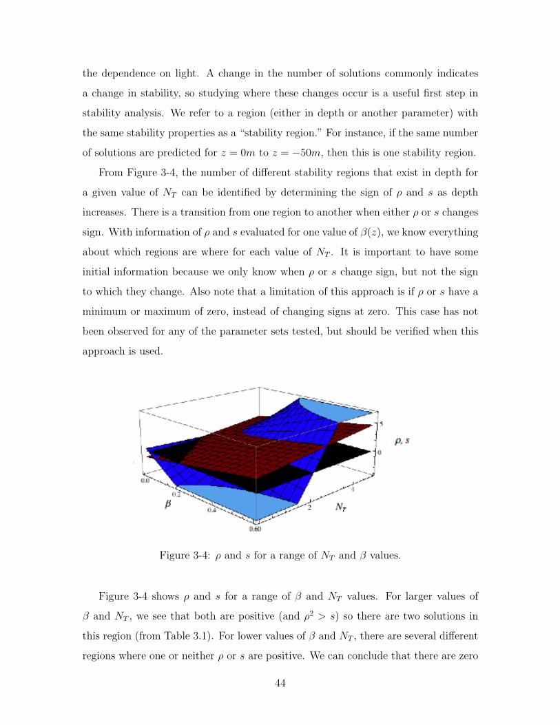
From Figure 3-4, the number of different stability regions that exist in depth for
a given value of NT can be identified by determining the sign of ρ and s as depth
increases. There is a transition from one region to another when either ρ or s changes
sign. With information of ρ and s evaluated for one value of β(z), we know everything
about which regions are where for each value of NT . It is important to have some
initial information because we only know when ρ or s change sign, but not the sign
to which they change. Also note that a limitation of this approach is if ρ or s have a
minimum or maximum of zero, instead of changing signs at zero. This case has not
been observed for any of the parameter sets tested, but should be verified when this
approach is used.
Figure 3-4: ρ and s for a range of NT and β values.
Figure 3-4 shows ρ and s for a range of β and NT values. For larger values of
β and NT , we see that both are positive (and ρ2 > s) so there are two solutions in
this region (from Table 3.1). For lower values of β and NT , there are several different
regions where one or neither ρ or s are positive. We can conclude that there are zero
44

Z equilibrium ρ > 0 when 0 ≤ β(z) ≤ βcρ ρ < 0 when βcρ ≤ β(z) ≤ u
s > 0 when 0 ≤ β(z) ≤ βcs 2 solutions if ρ2 > s No solutions1 solution if ρ2 < s
s < 0 when βcs ≤ β ≤ u 1 solution (positive branch) 1 solution (positive branch)
Table 3.1: Number of zooplankton equilibrium points with ρ, s, and β(z). βcs is thedepth where s changes sign and βcρ is the depth where ρ changes sign.
or one solutions in this region. All four combinations listed in Table 3.1 are possible,
as we can see in Figure 3-4.
While the three-dimensional plot is useful in providing a general idea of where
region transitions are for given values of β and NT , specific values of NT should be
examined to understand details of where region transitions occur. (This is done at
the end of this section, with results in Appendix A.) We define critical stability values
of depth as βcs and βcρ for a region transition (when s or ρ change sign, respectively).
They are expressed in terms of the system parameters, including NT :
βcs = dp
(ks +NT + γ
ν
)NT + γ
ν
βcρ = dp +dza
(1 +
ν
γ(ks +NT )
) (3.6)
These critical stability depths are then used to find the range of NT for which there
are different stability regions with different limits. The critical values of NT which
define these ranges are:
NTcρ = −(γ
ν
(dpa
dz+ 1
)+ ks
)NTcs = −NTcρ −
γ
ν
dpa
dz
(3.7)
Because γ is always negative, NTcs > NTcρ. The three different ranges of NT with
unique stability properties are shown in Table 3.2.
Table 3.2 is constructed using the critical stability values of Equations 3.6 and 3.7,
which indicate when a sign change of ρ or s occur, and Table 3.1, which determines
45

Region 1 Region 2 Region 3Z 0 ≤ β < βc1 βc1 < β < βc2 βc2 < β ≤ u
−∞ < z < zc1 zc1 < z < zc2 zc2 < z ≤ 0
s > 0 s < 0 s < 00 < NT < NTcρ ρ < 0 ρ < 0 ρ > 0
No solutions One solution One solutions < 0 s < 0 s < 0
NTcρ < NT < NTcs ρ < 0 ρ > 0 ρ > 0One solution One solution One solution
s < 0 s > 0 s > 0NT > NTcs ρ > 0 ρ > 0 ρ > 0
One solution Two solutions Two solutions
Table 3.2: Number of zooplankton equilibrium based on total biomass (NT ), depth,and the sign of ρ and s. βc1 and βc2 are chosen based on the values of βcρ and βcs.For instance, if βcρ > βcs, then βc1 = βcs and βc2 = βcρ.
NTcs = 2.31 βcs = 0.016 βcρ = 0.002NTcρ = 2.13 βcs = 0 βcρ = 0.036
Table 3.3: Critical values for parameter values listed in Equation 3.5, also presentedin Figure 3-5.
how many solutions of Z exist, given the sign of ρ and s. Table 3.2 assumes ρ > 0
and s > 0 for NT < NTcs for β = 0 as initial conditions. If this assumption is
not true, a similar table can easily be constructed using the above approach. The
critical values hold for any initial condition. These ideas are clarified with an example.
For the parameter values listed in Equation 3.5 the corresponding critical values are
presented in Table 3.3 and in Figures 3-5 and 3-6.
Figures 3-5 and 3-6 provide a new technique of examining the number of solutions
for different regions of NT . The values of β where solution properties change are as
predicted in Equation 3.6. Figure 3-5 is shown in terms of β and Figure 3-6 in terms
of z. Again, plotting the graph in terms of β allows us to describe the system more
generally, as the depth decay scale h and uptake rate u are not specified and are left
completely general.
Holding NT constant at NT = 2, 2.2, and 3 µmol/L (values above, in between,
and below the critical values that define the ranges of NT ) for the case shown in
46
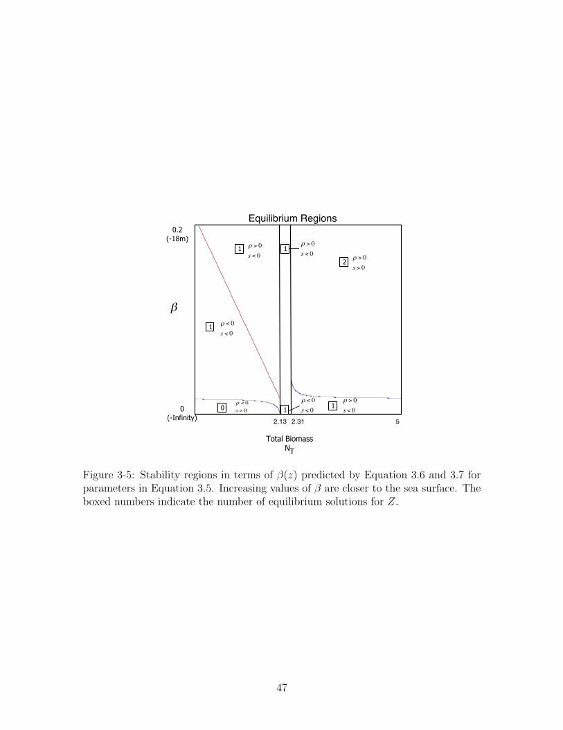
!"#$%&'(")$**
+!
,-.("/*&"0&1#$2(%(#3
!"#$ !"$# %
4
!
456
789:);
4
78</0(/(#3;
9
9 9
99
6
! ! !
! " !
! ! !
! ! !
! ! !
! " !
! ! !
! ! !
! ! !
! " !! ! !
! ! !
! ! !
! " !
Equilibrium Regions
Figure 3-5: Stability regions in terms of β(z) predicted by Equation 3.6 and 3.7 forparameters in Equation 3.5. Increasing values of β are closer to the sea surface. Theboxed numbers indicate the number of equilibrium solutions for Z.
47

!
"#$%&'()*
+,%-.'/0,)-11
2+
3#40,51',6'7%-80.0%9
!"#$ !"$# %
&'('
)*+,-./01
2#&&'(
! ! !
! ! !
! ! !
! " !
! ! !
! " !
:
;
;;
;
! ! !
! " !
! ! !
! ! !
;
<! ! !
! ! !
! ! !
! " !
Equilibrium Regions
Figure 3-6: Stability regions in terms of z predicted by Equation 3.6 and 3.7 forparameters in Equation 3.5. The boxed numbers indicate the number of equilibriumsolutions for Z.
48

Figure 3-5 are presented in Appendix A. The final figures of Appendix A show that
the number of solutions for Z predicted using Table 3.1 are correct. The last figure
also reveals that the positive root of Z never gives positive nutrient concentration
(for those parameter values used).
Being able to identify the values of depth β(z) and biomass NT where solutions
exist and defining the number of such equilibrium solutions is very powerful. Stability
properties may change at the transitions across regions. These ranges are specified
by the values of the equation parameters and bring us closer to identifying ranges of
parameters for stable solutions.
3.2 Stability of the Linearized System
Using the information about equilibria discussed in Section 3.1, an analysis of the
linearized equations (in the reference frame without physics) around the equilibria
solutions reveals stability properties for the general solution regions. Equations 3.1 are
linearized around the equilibria (P0 and Z0 from Equations 3.4, using the “negative”
Z root) and the result is a system of two ordinary differential equations:
dPdt
dZdt
≈ MPP MPZ
MZP MZZ
P0
Z0
(3.8)
where Mij is the linear coefficient of j for the i equation and is comprised entirely of
system parameters. For a local stability study, we focus on the matrix that describes
the first order behavior of the system (matrix M). The eigenvalues of the Jacobian of
Equation 3.8 indicates local stability: if the real part is positive, we expect unstable
behavior and if the real parts of both eigenvalues are negative, the solutions are stable.
If the real part of the eigenvalue is zero, an oscillatory solution results, assuming the
imaginary part of the eigenvalue is non-zero. Equation 3.9 is the Jacobian of the
linearized system, where P0 and Z0 are the equilibrium values.
49
J =
A11 A12
A21 A22
where
A11 = −dp − e−P0νgZ0 +ezhu(ks (NT − 2P0 − Z0) + (−NT + P0 + Z0)
2)(ks +NT − P0 − Z0)
2
A12 =
(−1 + e−P0ν
)g
ν− e
zhksP0u
(ks +NT − P0 − Z0)2
A21 = ae−P0νgZ0
A22 = −dz +a(1− e−P0ν
)g
ν
(3.9)
The corresponding eigenvalues of the Jacobian can be expressed in closed form
using the general expression for eigenvalues of a 2x2 matrix:
σ1 =1
2
(A11 + A22 −
√A2
11 + 4A12A21 − 2A11A22 + A222
)σ2 =
1
2
(A11 + A22 +
√A2
11 + 4A12A21 − 2A11A22 + A222
) (3.10)
Although we can see that the eigenvalues of the Jacobian can easily be expressed
in closed form from Equations 3.9 and 3.10, the result includes numerous terms. If
some system parameters are known, the effect of the range of the unknown parameter
values can be expressed analytically by taking the derivative of the eigenvalues with
respect to the unknown parameter. Identifying where the real part of the eigenvalue
is negative and positive gives defined ranges of stability and instability in terms of
the unknown parameter.
Using the parameters from Equation 3.5, we assume here that all parameters but
NT are known and perform the stability analysis for total biomass. In Chapter 4,
we initialize a two-dimensional simulation using a specified NT , so it is important to
know if a particular region (with a specific NT value) would give a stable or unstable
solution so as to anticipate the local behavior of the time-dependent solutions.
50
2 4 6 8 10
- 0.10
- 0.08
- 0.06
- 0.04
- 0.02
0.02
0.04
z=- 50m
z=- 35m
z=- 25m
z=- 15m
z=- 5m
z=0m
Real Eigenvalues for the Linearized System
NT
Re(σ)
Figure 3-7: Real part of the eigenvalues for the Jacobian of the linearized systemevaluated at the equilibrium with varying total biomass.
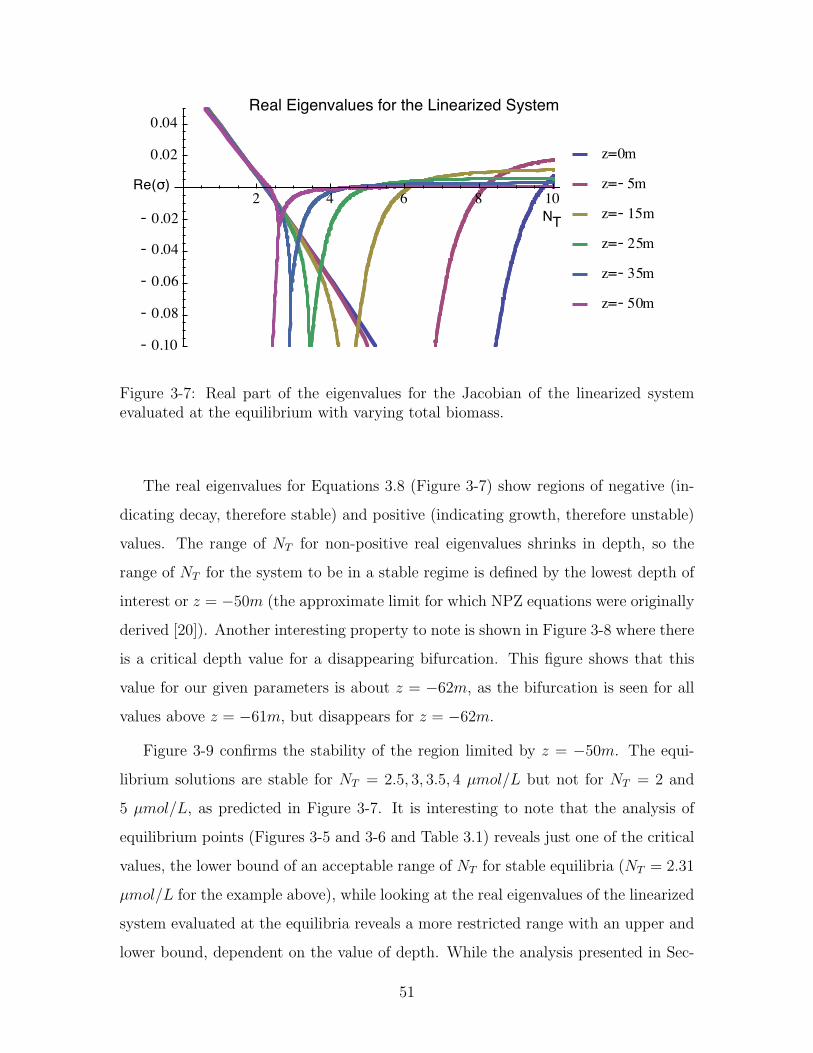
The real eigenvalues for Equations 3.8 (Figure 3-7) show regions of negative (in-
dicating decay, therefore stable) and positive (indicating growth, therefore unstable)
values. The range of NT for non-positive real eigenvalues shrinks in depth, so the
range of NT for the system to be in a stable regime is defined by the lowest depth of
interest or z = −50m (the approximate limit for which NPZ equations were originally
derived [20]). Another interesting property to note is shown in Figure 3-8 where there
is a critical depth value for a disappearing bifurcation. This figure shows that this
value for our given parameters is about z = −62m, as the bifurcation is seen for all
values above z = −61m, but disappears for z = −62m.
Figure 3-9 confirms the stability of the region limited by z = −50m. The equi-
librium solutions are stable for NT = 2.5, 3, 3.5, 4 µmol/L but not for NT = 2 and
5 µmol/L, as predicted in Figure 3-7. It is interesting to note that the analysis of
equilibrium points (Figures 3-5 and 3-6 and Table 3.1) reveals just one of the critical
values, the lower bound of an acceptable range of NT for stable equilibria (NT = 2.31
µmol/L for the example above), while looking at the real eigenvalues of the linearized
system evaluated at the equilibria reveals a more restricted range with an upper and
lower bound, dependent on the value of depth. While the analysis presented in Sec-
51
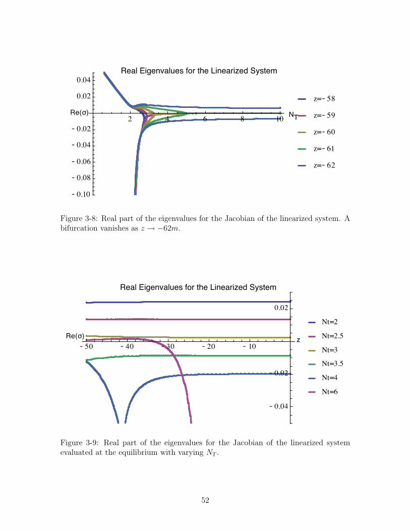
2 4 6 8 10
- 0.10
- 0.08
- 0.06
- 0.04
- 0.02
0.02
0.04
z=- 62
z=- 61
z=- 60
z=- 59
z=- 58
Real Eigenvalues for the Linearized System
NTRe(σ)
Figure 3-8: Real part of the eigenvalues for the Jacobian of the linearized system. Abifurcation vanishes as z → −62m.
- 50 - 40 - 30 - 20 - 10
- 0.04
- 0.02
0.02
Nt=6
Nt=4
Nt=3.5
Nt=3
Nt=2.5
Nt=2
Real Eigenvalues for the Linearized System
zRe(σ)
Figure 3-9: Real part of the eigenvalues for the Jacobian of the linearized systemevaluated at the equilibrium with varying NT .
52

tion 3.1 does provide useful information globally, it does not give us complete NT
ranges of local stability.
Figures 3-10 and 3-11 show identical analysis as presented for Figure 3-7 through
Figure 3-9, but now the Jacobian is evaluated at the positive root of the Z equilibrium
solution of Equations 3.4.
5 10 15 20
- 0.5
- 0.4
- 0.3
- 0.2
- 0.1
0.1
z=- 50
z=- 35
z=- 25
z=- 15
z=- 10
z=- 5
z=0
Real Eigenvalues for the Linearized System
NTRe(σ)
Figure 3-10: Real part of the eigenvalues for the Jacobian of the linearized systemevaluated at the equilibrium (positive Z root) with varying depth.
Unlike the previous case, the growth rates for the positive root of Z are limited by
z = 0m, not z = −50m. The critical lower bound NT value is 7.7 µmol/L. Beyond
this lower bound, there are positive growth rates. Figures 3-11 and 3-12 show that
all NT < 7.7 µmol/L have positive growth rates at the surface (z = 0m).
Those critical values for NT found in Section 3.2 do not reveal anything about the
stability properties of the linearized equations around the positive Z equation because
they described the transition of the negative Z root appearing or disappearing (see
Table 3.1). We focus on the “negative” root because the positive root of the Z
equilibrium is limited in producing real, positive values, while the negative Z root
gives physical results (Z > 0) more often for our parameter set. The stability regions
(in NT ) for both roots are summarized in Table 3.4.
Having a stable solution does not imply that it is a physical solution (real and
53
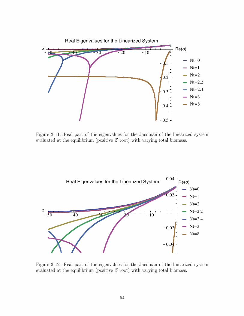
- 50 - 40 - 30 - 20 - 10
- 0.5
- 0.4
- 0.3
- 0.2
- 0.1
Nt=8
Nt=3
Nt=2.4
Nt=2.2
Nt=2
Nt=1
Nt=0
Real Eigenvalues for the Linearized System
z Re(σ)
Figure 3-11: Real part of the eigenvalues for the Jacobian of the linearized systemevaluated at the equilibrium (positive Z root) with varying total biomass.
- 50 - 40 - 30 - 20 - 10
- 0.04
- 0.02
0.02
0.04
Nt=8
Nt=3
Nt=2.4
Nt=2.2
Nt=2
Nt=1
Nt=0
Real Eigenvalues for the Linearized System
z
Re(σ)
Figure 3-12: Real part of the eigenvalues for the Jacobian of the linearized systemevaluated at the equilibrium (positive Z root) with varying total biomass.
54
Linearized Equations with: Z+ equil. pt. Z− equil. pt.
Stable if NT > 7.7 2.31 < NT < 4.44forzMAX = −50mUnstable if NT < 7.7 NT < 2.31orNT > 4.44forzMAX = −50m
Table 3.4: Stability regions (in total biomass, limited by z = 0) for parameter valueslisted in Equation 3.5.
positive). In fact, the last graph of Appendix A shows that the positive root of the
Z equilibrium never gives a positive N value. So, while the positive root of the Z
equilibrium may give stable results, they are not physical. An example is presented
in Figure 3-13. While both of these equilibrium solutions are within the stable regime
of NT and z, only the negative root is physical (positive for N,P, and Z).
2 4 6
- 50
- 40
- 30
- 20
- 10
0.5 1.0 1.5 2.0
- 50
- 40
- 30
- 20
- 10
NT=8, Positive root of Z equilibrium
Ȉ (umol/L)
zz
Ȉ (umol/L)
NT=3, Negative root of Z equilibrium
P
N
Z N Z P
Figure 3-13: Stability does not imply a physical solution. Though NT = 8 gives astable solution, it is unrealistic, with negative nutrient values.
Closed form expressions for stability ranges of parameters can be derived for ks, dp
and ν and the new above method we developed can be applied to analyze local
stability. The parameters dz, a and g do not give closed form solutions, but similar
analysis can be performed with the aid of numerical “root finding” schemes. These
expressions are shown in Table 3.5. The critical stability depths, βcs and βcρ, are
always in closed form.
The predictions of critical stability depths and stability regions in terms of NT
presented in this section are tested using phase portraits, which plot the evolution of
Equations 3.1 in time. These results are represented in the phase space, P versus Z.
The phase portraits allow us to verify our new predictions for equilibrium points and
55
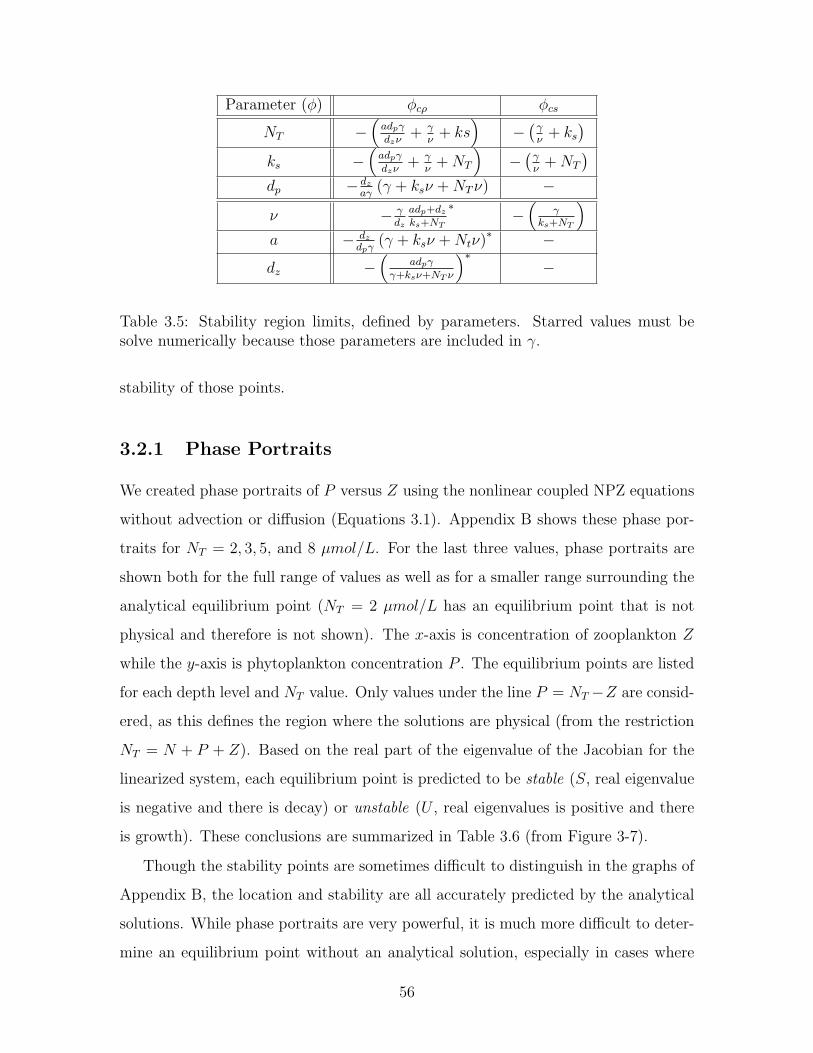
Parameter (φ) φcρ φcs
NT −(adpγ
dzν+ γ
ν+ ks
)−(γν
+ ks)
ks −(adpγ
dzν+ γ
ν+NT
)−(γν
+NT
)dp − dz
aγ(γ + ksν +NTν) −
ν − γdz
adp+dzks+NT
∗−(
γks+NT
)a − dz
dpγ(γ + ksν +Ntν)∗ −
dz −(
adpγ
γ+ksν+NT ν
)∗−
Table 3.5: Stability region limits, defined by parameters. Starred values must besolve numerically because those parameters are included in γ.
stability of those points.
3.2.1 Phase Portraits
We created phase portraits of P versus Z using the nonlinear coupled NPZ equations
without advection or diffusion (Equations 3.1). Appendix B shows these phase por-
traits for NT = 2, 3, 5, and 8 µmol/L. For the last three values, phase portraits are
shown both for the full range of values as well as for a smaller range surrounding the
analytical equilibrium point (NT = 2 µmol/L has an equilibrium point that is not
physical and therefore is not shown). The x-axis is concentration of zooplankton Z
while the y-axis is phytoplankton concentration P . The equilibrium points are listed
for each depth level and NT value. Only values under the line P = NT −Z are consid-
ered, as this defines the region where the solutions are physical (from the restriction
NT = N + P + Z). Based on the real part of the eigenvalue of the Jacobian for the
linearized system, each equilibrium point is predicted to be stable (S, real eigenvalue
is negative and there is decay) or unstable (U , real eigenvalues is positive and there
is growth). These conclusions are summarized in Table 3.6 (from Figure 3-7).
Though the stability points are sometimes difficult to distinguish in the graphs of
Appendix B, the location and stability are all accurately predicted by the analytical
solutions. While phase portraits are very powerful, it is much more difficult to deter-
mine an equilibrium point without an analytical solution, especially in cases where
56
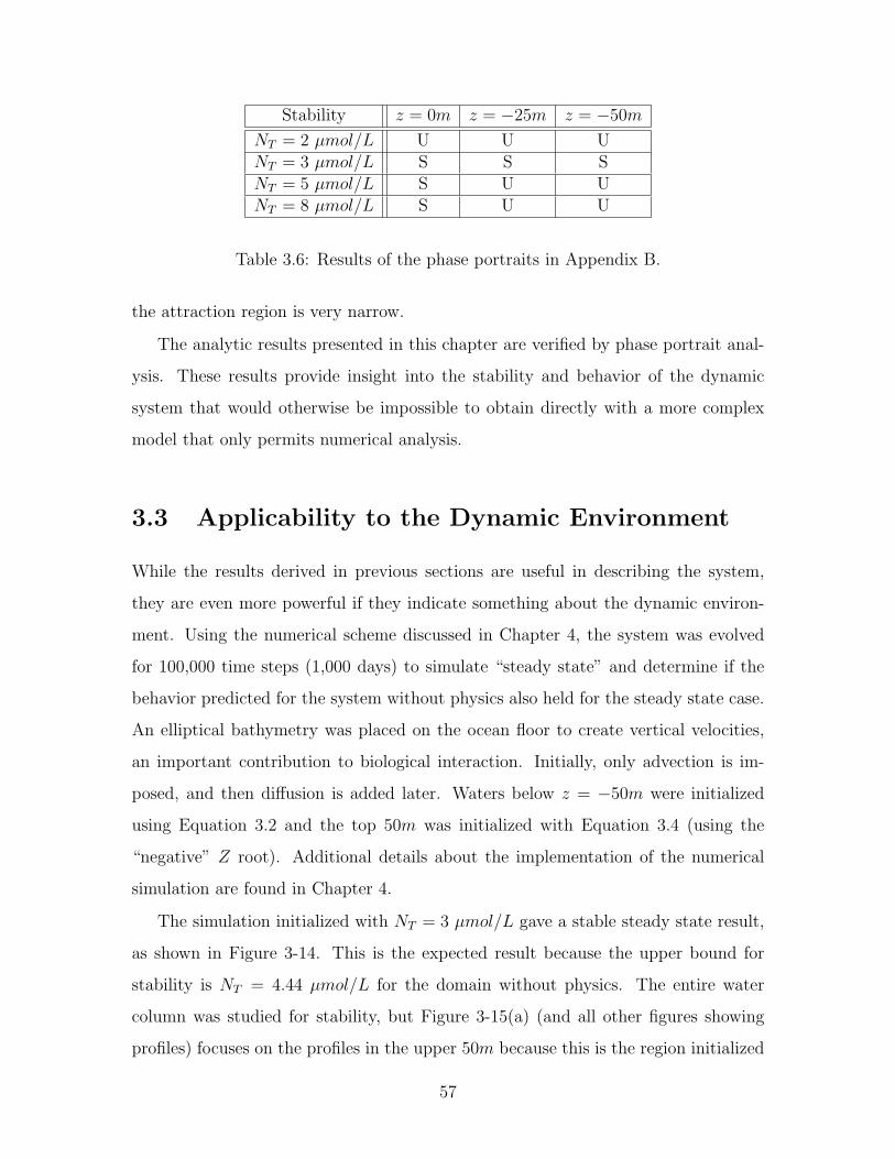
Stability z = 0m z = −25m z = −50m
NT = 2 µmol/L U U UNT = 3 µmol/L S S SNT = 5 µmol/L S U UNT = 8 µmol/L S U U
Table 3.6: Results of the phase portraits in Appendix B.
the attraction region is very narrow.
The analytic results presented in this chapter are verified by phase portrait anal-
ysis. These results provide insight into the stability and behavior of the dynamic
system that would otherwise be impossible to obtain directly with a more complex
model that only permits numerical analysis.
3.3 Applicability to the Dynamic Environment
While the results derived in previous sections are useful in describing the system,
they are even more powerful if they indicate something about the dynamic environ-
ment. Using the numerical scheme discussed in Chapter 4, the system was evolved
for 100,000 time steps (1,000 days) to simulate “steady state” and determine if the
behavior predicted for the system without physics also held for the steady state case.
An elliptical bathymetry was placed on the ocean floor to create vertical velocities,
an important contribution to biological interaction. Initially, only advection is im-
posed, and then diffusion is added later. Waters below z = −50m were initialized
using Equation 3.2 and the top 50m was initialized with Equation 3.4 (using the
“negative” Z root). Additional details about the implementation of the numerical
simulation are found in Chapter 4.
The simulation initialized with NT = 3 µmol/L gave a stable steady state result,
as shown in Figure 3-14. This is the expected result because the upper bound for
stability is NT = 4.44 µmol/L for the domain without physics. The entire water
column was studied for stability, but Figure 3-15(a) (and all other figures showing
profiles) focuses on the profiles in the upper 50m because this is the region initialized
57

with the equilibrium solution of interest. Figure 3-15(a) shows the profiles for each
node in the horizontal dimension in the domain at steady state for all three state
variables. From these profiles, we see no evidence of unstable behavior. Figure 3-
15(b) would show cross-hatching at any depth where an unstable solution is predicted
for the domain without physics, but the euphotic zone is entirely stable in this case.
Lastly, Figure 3-15 presents the real eigenvalues for NT = 3 µmol/L in the domain
without physics. In this case, they are all negative.
Figure 3-14: Steady state solution (for advection only) for nutrient, phytoplankton,and zooplankton for initial biomass of NT = 3 µmol/L.
58
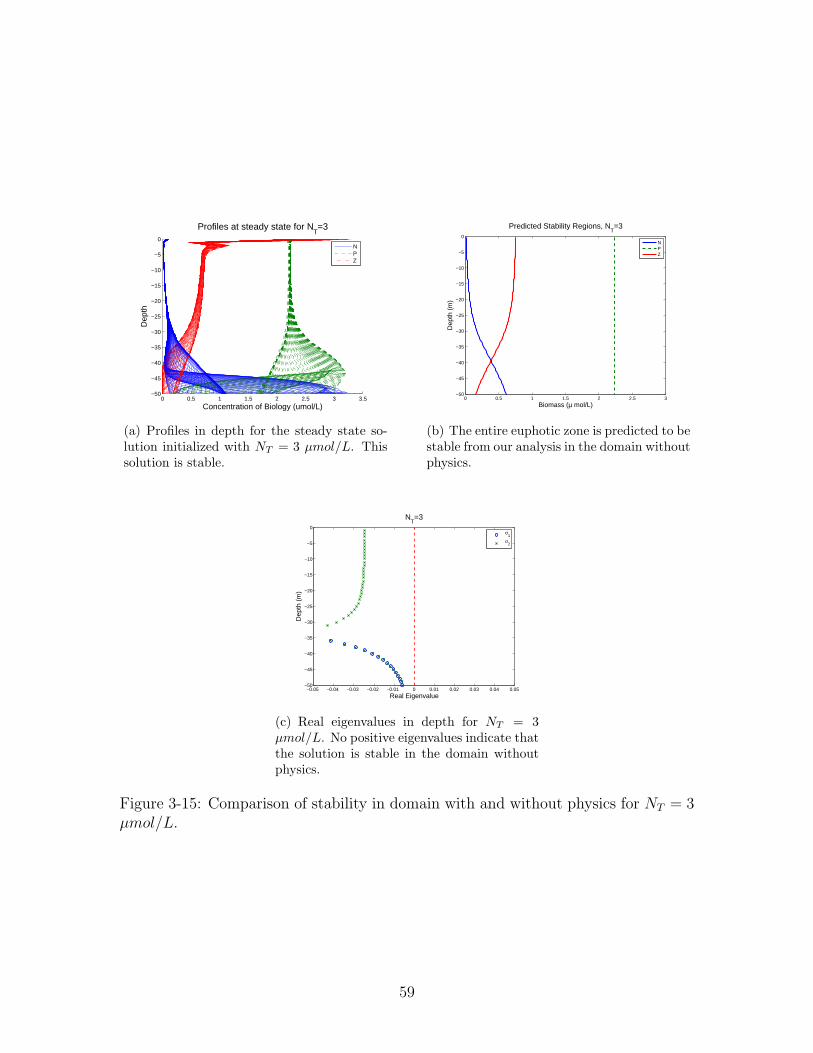
0 0.5 1 1.5 2 2.5 3 3.5−50
−45
−40
−35
−30
−25
−20
−15
−10
−5
0
Concentration of Biology (umol/L)
Dep
th
Profiles at steady state for NT=3
NPZ
(a) Profiles in depth for the steady state so-lution initialized with NT = 3 µmol/L. Thissolution is stable.
0 0.5 1 1.5 2 2.5 3−50
−45
−40
−35
−30
−25
−20
−15
−10
−5
0
Predicted Stability Regions, NT=3
Biomass (µ mol/L)
Dep
th (
m)
NPZ
(b) The entire euphotic zone is predicted to bestable from our analysis in the domain withoutphysics.
−0.05 −0.04 −0.03 −0.02 −0.01 0 0.01 0.02 0.03 0.04 0.05−50
−45
−40
−35
−30
−25
−20
−15
−10
−5
0
Real Eigenvalue
Dep
th (
m)
NT=3
σ
1
σ2
(c) Real eigenvalues in depth for NT = 3µmol/L. No positive eigenvalues indicate thatthe solution is stable in the domain withoutphysics.
Figure 3-15: Comparison of stability in domain with and without physics for NT = 3µmol/L.
59
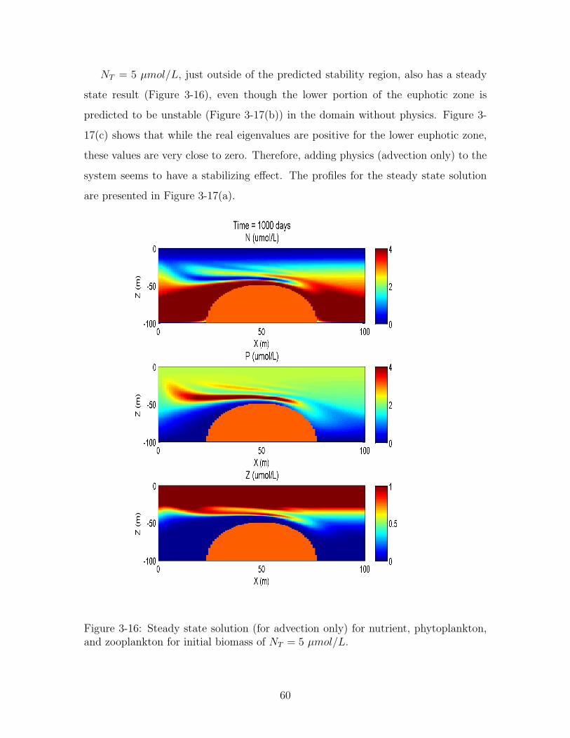
NT = 5 µmol/L, just outside of the predicted stability region, also has a steady
state result (Figure 3-16), even though the lower portion of the euphotic zone is
predicted to be unstable (Figure 3-17(b)) in the domain without physics. Figure 3-
17(c) shows that while the real eigenvalues are positive for the lower euphotic zone,
these values are very close to zero. Therefore, adding physics (advection only) to the
system seems to have a stabilizing effect. The profiles for the steady state solution
are presented in Figure 3-17(a).
Figure 3-16: Steady state solution (for advection only) for nutrient, phytoplankton,and zooplankton for initial biomass of NT = 5 µmol/L.
60
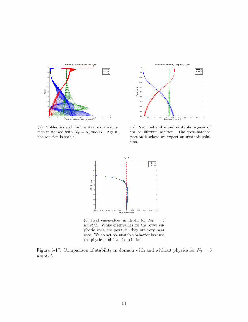
0 1 2 3 4 5 6 7 8−50
−45
−40
−35
−30
−25
−20
−15
−10
−5
0
Concentration of Biology (umol/L)
Dep
th
Profiles at steady state for NT=5
NPZ
(a) Profiles in depth for the steady state solu-tion initialized with NT = 5 µmol/L. Again,the solution is stable.
0 0.5 1 1.5 2 2.5 3 3.5 4 4.5 5−50
−45
−40
−35
−30
−25
−20
−15
−10
−5
0
Predicted Stability Regions, NT=5
Biomass (µ mol/L)
Dep
th (
m)
NPZ
(b) Predicted stable and unstable regimes ofthe equilibrium solution. The cross-hatchedportion is where we expect an unstable solu-tion.
−0.05 −0.04 −0.03 −0.02 −0.01 0 0.01 0.02 0.03 0.04 0.05−50
−45
−40
−35
−30
−25
−20
−15
−10
−5
0
Real Eigenvalue
Dep
th (
m)
NT=5
σ
1
σ2
(c) Real eigenvalues in depth for NT = 5µmol/L. While eigenvalues for the lower eu-photic zone are positive, they are very nearzero. We do not see unstable behavior becausethe physics stabilize the solution.
Figure 3-17: Comparison of stability in domain with and without physics for NT = 5µmol/L.
61

Domains with more total biomass in the system have higher real positive eigen-
values (Figure 3-19(c)), so their growth rate becomes larger as NT grows. A steady
state solution was not found for NT = 12 µmol/L (Figure 3-18) because values near
the surface were oscillatory. The profiles for the state at 100,000 time steps, or 1,000
days, (Figure 3-19(a)) show very noisy values of biology near the surface, due to the
unstable nature of this case. Note the physical and biological time scales are com-
parable: it takes 25 days for the mean flow to advect over the bathymetry, while
the time scale for biological reaction is about 30 days. As Figure 3-19(b) shows, the
entire euphotic zone is predicted to be unstable in the domain without physics, with
real eigenvalues much larger than in the previous case, as shown in Figure 3-19(c).
Therefore, while rapid growth does not occur for large NT values, solutions are likely
unphysical and our stability analysis in the domain without physics gives us a conser-
vative estimate of appropriate values of total biomass to use for the system to remain
stable. While regions with very small real eigenvalues stabilized when advection was
added, larger positive real eigenvalues did not. While it is possible for the biology to
become unstable, at least for some short period of time, knowing these limitations by
examining the parameters in the domain without physics is powerful. When physics
are added, it can become challenging to distinguish which effects are due to biological
reactions and which are due to the interaction of physics and biology.
We expect diffusion to have a stabilizing effect. Performing an identical simulation
with NT = 12 µmol/L, but now including a diffusion constant of κ = 0.1 in the x−
and z−direction, we obtain Figure 3-20. Comparing the profiles of this case (Figure
3-21) to the case without diffusion (Figure 3-19(a)) reveals that the oscillations have
subsided because of the diffusion introduced in the system and a steady state is
attainable (Figure 3-20).
3.4 Discussion
Steady equilibria for an NPZ model were found and used to determine relationships
between critical stability depth, biomass, and the number of positive, real solutions
62
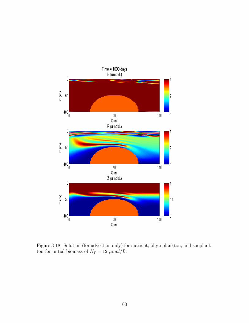
Figure 3-18: Solution (for advection only) for nutrient, phytoplankton, and zooplank-ton for initial biomass of NT = 12 µmol/L.
63

0 5 10 15−50
−45
−40
−35
−30
−25
−20
−15
−10
−5
0
Concentration of Biology (umol/L)
Dep
th
Profiles at steady state for NT=12
NPZ
(a) Profiles in depth for the solution initializedwith NT = 12 after 100,000 time steps (1,000days). The oscillatory behavior about −20mindicates unstable behavior. No steady statesolution was found for this case.
0 2 4 6 8 10 12−50
−45
−40
−35
−30
−25
−20
−15
−10
−5
0
Predicted Stability Regions, NT=12
Biomass (µ mol/L)
Dep
th (
m)
NPZ
(b) The entire euphotic zone was predicted tobe unstable for NT = 12 µmol/L.
−0.05 −0.04 −0.03 −0.02 −0.01 0 0.01 0.02 0.03 0.04 0.05−50
−45
−40
−35
−30
−25
−20
−15
−10
−5
0
Real Eigenvalue
Dep
th (
m)
NT=12
σ
1
σ2
(c) Real eigenvalues in depth for NT = 12µmol/L. The magnitude of the real eigenval-ues decay in depth. Comparing this figure toFigure 3-19(a), it seems that adding physicsto a domain can stabilize real eigenvalue ofabout 0.01 and below, but any value greaterthan this led to unstable behavior.
Figure 3-19: Comparison of stability in domain with and without physics for NT = 12µmol/L.
64
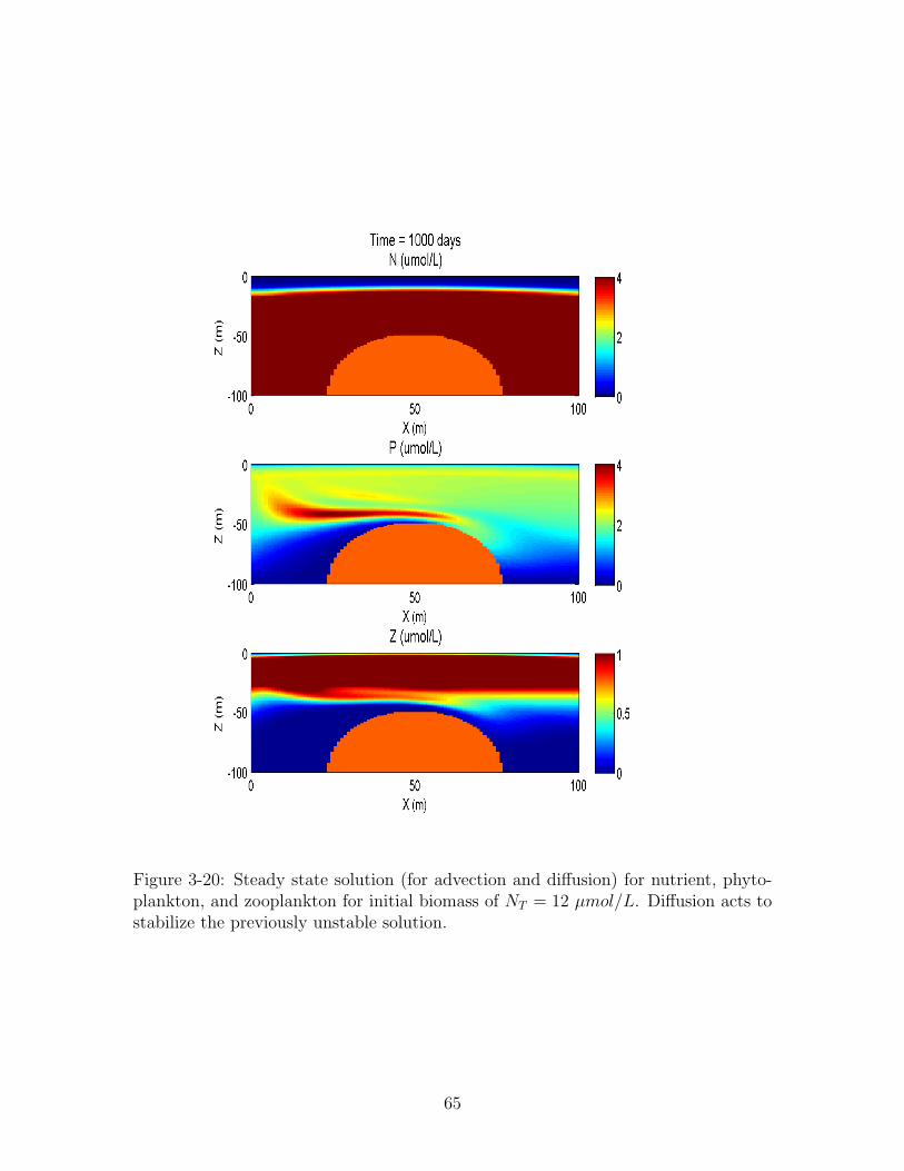
Figure 3-20: Steady state solution (for advection and diffusion) for nutrient, phyto-plankton, and zooplankton for initial biomass of NT = 12 µmol/L. Diffusion acts tostabilize the previously unstable solution.
65
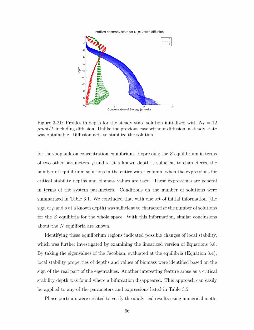
0 5 10 15−50
−45
−40
−35
−30
−25
−20
−15
−10
−5
0
Concentration of Biology (umol/L)
Dep
th
Profiles at steady state for NT=12 with diffusion
NPZ
Figure 3-21: Profiles in depth for the steady state solution initialized with NT = 12µmol/L including diffusion. Unlike the previous case without diffusion, a steady statewas obtainable. Diffusion acts to stabilize the solution.
for the zooplankton concentration equilibrium. Expressing the Z equilibrium in terms
of two other parameters, ρ and s, at a known depth is sufficient to characterize the
number of equilibrium solutions in the entire water column, when the expressions for
critical stability depths and biomass values are used. These expressions are general
in terms of the system parameters. Conditions on the number of solutions were
summarized in Table 3.1. We concluded that with one set of initial information (the
sign of ρ and s at a known depth) was sufficient to characterize the number of solutions
for the Z equilibria for the whole space. With this information, similar conclusions
about the N equilibria are known.
Identifying these equilibrium regions indicated possible changes of local stability,
which was further investigated by examining the linearized version of Equations 3.8.
By taking the eigenvalues of the Jacobian, evaluated at the equilibria (Equation 3.4),
local stability properties of depths and values of biomass were identified based on the
sign of the real part of the eigenvalues. Another interesting feature arose as a critical
stability depth was found where a bifurcation disappeared. This approach can easily
be applied to any of the parameters and expressions listed in Table 3.5.
Phase portraits were created to verify the analytical results using numerical meth-
66
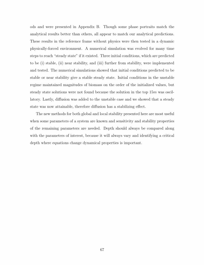
ods and were presented in Appendix B. Though some phase portraits match the
analytical results better than others, all appear to match our analytical predictions.
These results in the reference frame without physics were then tested in a dynamic
physically-forced environment. A numerical simulation was evolved for many time
steps to reach “steady state” if it existed. Three initial conditions, which are predicted
to be (i) stable, (ii) near stability, and (iii) further from stability, were implemented
and tested. The numerical simulations showed that initial conditions predicted to be
stable or near stability give a stable steady state. Initial conditions in the unstable
regime maintained magnitudes of biomass on the order of the initialized values, but
steady state solutions were not found because the solution in the top 15m was oscil-
latory. Lastly, diffusion was added to the unstable case and we showed that a steady
state was now attainable, therefore diffusion has a stabilizing effect.
The new methods for both global and local stability presented here are most useful
when some parameters of a system are known and sensitivity and stability properties
of the remaining parameters are needed. Depth should always be compared along
with the parameters of interest, because it will always vary and identifying a critical
depth where equations change dynamical properties is important.
67

68
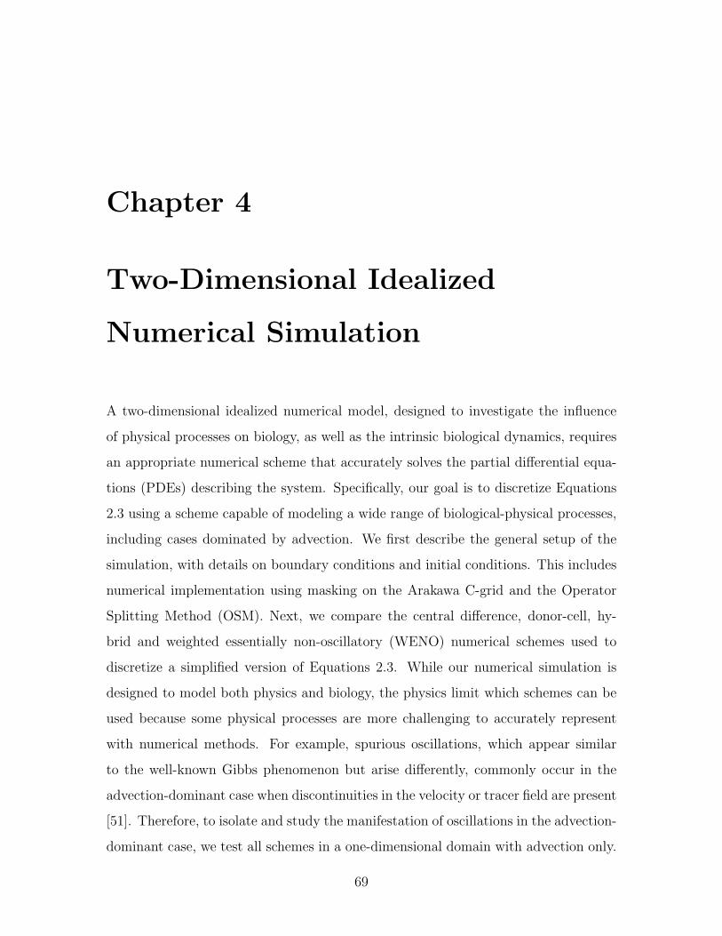
Chapter 4
Two-Dimensional Idealized
Numerical Simulation
A two-dimensional idealized numerical model, designed to investigate the influence
of physical processes on biology, as well as the intrinsic biological dynamics, requires
an appropriate numerical scheme that accurately solves the partial differential equa-
tions (PDEs) describing the system. Specifically, our goal is to discretize Equations
2.3 using a scheme capable of modeling a wide range of biological-physical processes,
including cases dominated by advection. We first describe the general setup of the
simulation, with details on boundary conditions and initial conditions. This includes
numerical implementation using masking on the Arakawa C-grid and the Operator
Splitting Method (OSM). Next, we compare the central difference, donor-cell, hy-
brid and weighted essentially non-oscillatory (WENO) numerical schemes used to
discretize a simplified version of Equations 2.3. While our numerical simulation is
designed to model both physics and biology, the physics limit which schemes can be
used because some physical processes are more challenging to accurately represent
with numerical methods. For example, spurious oscillations, which appear similar
to the well-known Gibbs phenomenon but arise differently, commonly occur in the
advection-dominant case when discontinuities in the velocity or tracer field are present
[51]. Therefore, to isolate and study the manifestation of oscillations in the advection-
dominant case, we test all schemes in a one-dimensional domain with advection only.
69

Additionally, we study numerical diffusion, which is particularly important when
modeling biological processes because an accurate solution cannot be found if the
reaction and diffusion terms are affected by numerical errors.
In this chapter, we focus on determining the most appropriate scheme to mini-
mize spurious oscillations with low computational costs and low numerical diffusion by
comparing several numerical schemes. The numerical diffusion and oscillatory nature
of the schemes are studied. Numerical diffusion is diffusion introduced from discretiz-
ing the differential equations which causes the system to behave differently than the
intended physical system. A comparison of several schemes reveals that the WENO
scheme is the most suitable for the idealized simulations. The resulting simulation is
verified against a simulation using Discontinuous Galerkin on an unstructured grid
with identical conditions.
4.1 Problem Setup
Equations 2.3 are discretized in a two-dimensional vertical “slice” of the ocean strait
(where x is the horizontal dimension and z is the vertical dimension). Any smooth
bathymetry can be implemented. By assuming a two-dimensional inviscid, incom-
pressible field, we can obtain a velocity field by solving the potential flow for any
particular bathymetry. Because we ignore viscosity, we do not expect the solution
near the sea bottom to be realistic, as there will be no boundary layer. Solving po-
tential flow ensures that the flow satisfies continuity and assumes no flow may exit
the sea surface or sea bottom. Code to solve for potential flow was developed by
Ueckermann [58]. Once the numerical simulation is verified for a potential velocity
field, other realistic flow fields can be used. For instance, taking a representative
averaged flow through a strait generated from the primitive equations using MSEAS
can be implemented to obtain a more realistic simulation.
70

4.1.1 Operator Splitting Method
The Operator Splitting Method (OSM) allows us to decouple problems and solve the
equations in a single dimension. OSM, also known as time splitting or the method of
fractional steps, is used to solve partial differential equations for initial value problems,
usually in multidimensions [46]. If an initial boundary value problem can be expressed
as a linear sum of operators (the operators themselves are not restricted to be linear),
the original PDE can be split into terms based on these operators. The operators are
applied to φ (the tracer, or in our case, biological concentration of a state variable)
additively, yet this does not restrict the PDE itself to be linear [61]. For Equation
2.3, the advection and diffusion terms are discretized and solved in one direction (x)
only, with the resulting solution of this step serving as the initial condition for the
terms in the alternate direction (z). This process is repeated for each time step. OSM
significantly reduces the computational cost by enabling us to solve the PDE in small
time steps in a single direction only [46], allowing us to use banded algorithms. The
OSM is limited in that it is most useful if the boundaries can be represented as a
simple geometry, a restraint already present due to using a structured grid. Only
boundaries that can be expressed as strictly perpendicular to one of the two axes (x
and z) can be represented exactly.
4.1.2 Boundary and Initial Conditions
Boundary conditions are selected to be periodic in the x-direction, so that all biology
leaving the system on one side enters the system on the other. For the sea surface
boundary, a Neumann no flux boundary condition is imposed. Additionally, a Neu-
mann boundary condition is implemented on the bathymetry. Therefore, because we
have no flux conditions at the top and bottom boundaries and periodic boundaries on
the sides, no biology leaves or enters the system. These boundary conditions create
a conservative system: the initial total biomass NT will remain constant for all time.
Initial conditions are the steady equilibria of the NPZ equations without flow,
Equations 3.4. These equilibria are discussed in Chapter 3 and shown in Figure 4-1.
71
Figure 4-1: Initial conditions for nutrients, phytoplankton, and zooplankton.
72

4.1.3 Bathymetry, Masking, and the C-grid
An Arakawa C-grid is a staggered grid that simplifies enforcement of the continuity
of mass by specifying separate node locations for the horizontal velocity, the verti-
cal velocity, and the concentration a of biological state variable (the tracer) [4]. In
this chapter, tracer and concentration of biological state variable will be used inter-
changeably. Space between nodes is constant in the grid, as shown in Figure 4-2.
For this setup, there are I nodes in the horizontal direction and J nodes vertically.
Node numbering begins at the top right corner and is separate for each type of node
(vertical velocity, horizontal velocity, and the tracer), so that there are IxJ nodes of
each type. φi,j refers to the tracer node that is ith from the left, jth from the top.
Using a C-grid allows boundary conditions to be implemented easily by applying
a masking technique. First, three masks are constructed by identifying which tracer
nodes lie under the bathymetry. For the C-grid, each mask is a IxJ matrix of ones
and zeros. These masks are later applied to the gradient and divergence operators of
the partial differential equation to enforce boundary conditions.
The three masks created “mask” all nodes under the bathymetry and any node
neighboring those masked tracer nodes [37]. These masks are constructed as follows:
the first mask corresponds to the tracer nodes and is called the tracer mask (MT ).
Zeros are placed at any tracer node under the bathymetry, while the remaining nodes
are given a value of one. For Figure 4-2, the six circular nodes behind the striped
area are masked (assigned a value of zero) and all other circular nodes are one, as
shown in Figure 4-3. To construct the horizontal velocity mask (MH), MT is shifted
in the positive x-direction one node and multiplied by itself, so that the result is an
IxJ matrix with the nodes surrounding the masked tracer nodes in the horizontal
direction assigned zeros and all other entries assigned ones. Again using the elliptical
bathymetry from Figure 4-2, nine square nodes are given zeros. All horizontal nodes
neighboring “masked” tracer nodes are now masked. Similarly, to create the vertical
velocity mask (MV ), MT is shifted down and multiplied by itself. The vertical velocity
mask does not differ from the tracer mask (in this case) because of how the nodes
73
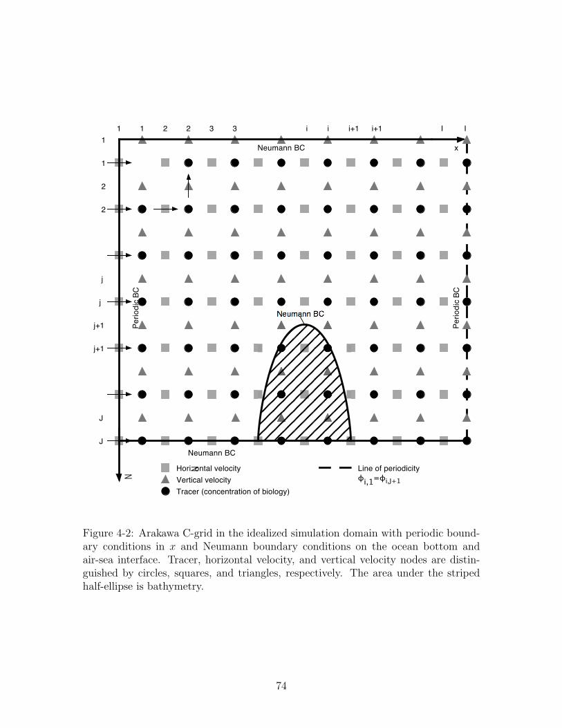
1 2 i I
1
2
j
J
3
Vertical velocity
Horizontal velocity
Tracer (concentration of biology)
x
z
Periodic BC
Periodic BC
Neumann BC
Neumann BC
Neumann BC
2 i+1 i
Line of periodicity
ϕi,1=ϕi,J+1
1
1
2
3 i+1 I
j
J
j+1
j+1
Figure 4-2: Arakawa C-grid in the idealized simulation domain with periodic bound-ary conditions in x and Neumann boundary conditions on the ocean bottom andair-sea interface. Tracer, horizontal velocity, and vertical velocity nodes are distin-guished by circles, squares, and triangles, respectively. The area under the stripedhalf-ellipse is bathymetry.
74
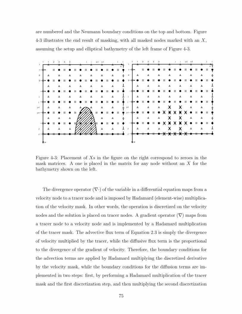
are numbered and the Neumann boundary conditions on the top and bottom. Figure
4-3 illustrates the end result of masking, with all masked nodes marked with an X,
assuming the setup and elliptical bathymetry of the left frame of Figure 4-3.
1 2 i I
1
2
j
J
3
x
z
2 i+1 i 1
1
2
3 i+1 I
j
J
j+1
j+1 X X
XX
XXX
X
X
XX
X
X
X
X
X
X X
X
X
X
1 2 i I
1
2
j
J
3
x
z
2 i+1 i 1
1
2
3 i+1 I
j
J
j+1
j+1
Figure 4-3: Placement of Xs in the figure on the right correspond to zeroes in themask matrices. A one is placed in the matrix for any node without an X for thebathymetry shown on the left.
The divergence operator (∇·) of the variable in a differential equation maps from a
velocity node to a tracer node and is imposed by Hadamard (element-wise) multiplica-
tion of the velocity mask. In other words, the operation is discretized on the velocity
nodes and the solution is placed on tracer nodes. A gradient operator (∇) maps from
a tracer node to a velocity node and is implemented by a Hadamard multiplication
of the tracer mask. The advective flux term of Equation 2.3 is simply the divergence
of velocity multiplied by the tracer, while the diffusive flux term is the proportional
to the divergence of the gradient of velocity. Therefore, the boundary conditions for
the advection terms are applied by Hadamard multiplying the discretized derivative
by the velocity mask, while the boundary conditions for the diffusion terms are im-
plemented in two steps: first, by performing a Hadamard multiplication of the tracer
mask and the first discretization step, and then multiplying the second discretization
75
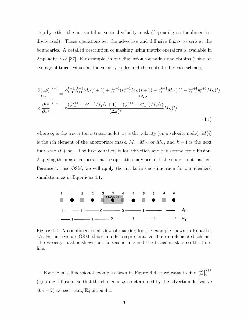
step by either the horizontal or vertical velocity mask (depending on the dimension
discretized). These operations set the advective and diffusive fluxes to zero at the
boundaries. A detailed description of masking using matrix operators is available in
Appendix B of [37]. For example, in one dimension for node i one obtains (using an
average of tracer values at the velocity nodes and the central difference scheme):
∂(uφ)
∂x
∣∣∣∣k+1
i
=φk+1i+1 u
k+1i+1MH(i+ 1) + φk+1
i (uk+1i+1MH(i+ 1)− uk+1
i MH(i))− φk+1i−1 u
k+1i MH(i)
2∆x
κ∂2φ
∂x2
∣∣∣∣k+1
i
= κ(φk+1
i+1 − φk+1i )MT (i+ 1)− (φk+1
i − φk+1i−1 )MT (i)
(∆x)2MH(i)
(4.1)
where φi is the tracer (on a tracer node), ui is the velocity (on a velocity node), M(i)
is the ith element of the appropriate mask, MT , MH , or MV , and k + 1 is the next
time step (t + dt). The first equation is for advection and the second for diffusion.
Applying the masks ensures that the operation only occurs if the node is not masked.
Because we use OSM, we will apply the masks in one dimension for our idealized
simulation, as in Equations 4.1.
! ! " " # # $ $ % % & &
''()*+,-
1 1 0 0 1 1
111011
MH
MT
Figure 4-4: A one-dimensional view of masking for the example shown in Equation4.2. Because we use OSM, this example is representative of our implemented scheme.The velocity mask is shown on the second line and the tracer mask is on the thirdline.
For the one-dimensional example shown in Figure 4-4, if we want to find ∂φ∂t
∣∣k+1
2
(ignoring diffusion, so that the change in φ is determined by the advection derivative
at i = 2) we see, using Equation 4.1:
76

∂φ
∂t
∣∣∣∣k+1
2
= − ∂(uφ)
∂x
∣∣∣∣k+1
2
= −(φk+1
3 uk+13 + φk+1
2 (uk+13 − uk+1
2 )− φk+11 uk+1
2
2∆xMH(2)
)with MH(2) = 1 and uk+1
3 = φk+13 = 0 so that
∂φ
∂t
∣∣∣∣k+1
2
= uk+12
(φk+1
2 + φk+11
2∆x
)(4.2)
We know that the tracer (φ) is always non-negative (because our tracer is concen-
tration of biology) and that velocity (u) can be either positive or negative. Therefore,
when the velocity node to the right of a tracer node is masked, the change of φ in time
increases (decreases) with the magnitude of the positive (negative) velocity times the
average concentration of biology at that velocity node, as expected.
4.2 Comparison of Numerical Schemes
With the problem setup complete, we compare numerical schemes by testing each in
both the two-dimensional domain just described and a one-dimensional domain. The
two-dimensional test cases reveals an overall view of features in the domain and the
one-dimensional case allows us to isolate and more clearly understand the specifics
of each scheme. Any features seen in the solution should be from the evolution of
the equations, not an artifact of the numerics. Spurious oscillations are common near
discontinuities in the advection-dominant case, so all test cases focus on how well
the schemes represent advection only. Therefore, there is no diffusion or interaction
between biology in any of the figures in this section. We are focused on representing
the following equation, which is a simplified version of Equations 2.3 without diffusion
or biological interaction:∂φ
∂t= −∂(uφ)
∂x− ∂(wφ)
∂z(4.3)
We have already discussed stability of the biological terms in Chapter 3 and it is
well known that adding diffusion stabilizes a system, so the best scheme to represent
77
Equations 4.3 will also be the best scheme to represent Equations 2.3 (our NPZ
equations with advection, diffusion and biological reaction terms). In the remainder
of this chapter, we show that the WENO scheme outperforms the central difference,
donor-cell scheme and hybrid schemes in preserving the behavior and physics of the
system. For each of the schemes discussed, we first examine the two-dimensional case,
then a one-dimensional case to test the scheme in a “worst-case” scenario, and lastly
we compare the cost efficiency of the schemes that accurately represent the modeled
dynamics.
4.2.1 One-dimensional and Two-dimensional Test Cases
To compare numerical schemes, a one-dimensional test case was created. By mask-
ing a single node, the boundary conditions and masking of the more general case
are tested. An initial Gaussian distribution is advected in the positive x direction
and encounters a “blocked” node at one-third the domain length from the leftmost
boundary (x = −17 in Figure 4-5). The boundary condition in x is periodic and 200
nodes are used to represent the domain. This test case uses a one-dimensional version
of Equation 4.3 and the initial setup is shown in Figure 4-5.
Because this test case is one-dimensional with periodic boundary conditions and
a blocked node, all of the tracer concentration initialized in the system should accu-
mulate against the blocked node. This is one of the most challenging cases to model
numerically because the tracer values at neighboring nodes are very different, which,
for many schemes, leads to spurious oscillations at these discontinuities.
The two-dimensional test case uses the setup described in Section 4.1.2 with 100
nodes in both x and z. The initial field is shown in Figure 4-6.
4.2.2 Central Difference Scheme
A second-order central difference scheme (CDS), implicit in time, is frequently used
in discretizing PDEs because it is higher order accurate, simple to implement, and
more stable than its time-explicit counterpart. A two-dimensional simulation with
78

!!" !#" !$" !%" !&" " &" %" $" #" !"
!"'(
!"'#
!"'%
"
"'%
"'#
"'(
)*+,+-./01*2+,+1*/314/&5/0-67
8
/
/
)*+,+-./01*2+,+1*
9-6:72/;127
u
Figure 4-5: Initial condition for the one-dimensional test case.
x
z
Initial Condition N field
10 20 30 40 50 60 70 80 90 100
10
20
30
40
50
60
70
80
90
100 0
0.5
1
1.5
2
2.5
3
Figure 4-6: Initial condition for the two-dimensional test case.
79

advection and sufficient diffusion did not reveal any physically unrealistic features.
However, in an identical simulation without diffusion, oscillations quickly formed at
the bathymetry boundary, as in Figure 4-7. After more time, the maximum and
minimum values reached several orders of magnitude above and below zero, respec-
tively. When the bathymetry was removed, CDS with advection only did not create
unrealistic results.
x
z
N field at timestep=500 using CDS
10 20 30 40 50 60 70 80 90 100
10
20
30
40
50
60
70
80
90
100 0
0.5
1
1.5
2
2.5
3
Figure 4-7: Central difference scheme in two dimensions. Spurious oscillations format the bathymetry boundary.
Figure 4-5 shows the initial distribution (dashed line) of the one-dimensional case
and the state after one cycle, or the time for a particle to advect around the do-
main exactly once (2010 time steps). The distribution is advected at a rate of five
length units per time unit. Again, we expect all of the concentration in the system
to accumulate in the node just before the masked node, leading to an impulse-type
distribution. Instead, as we see in Figure 4-8, as soon as a small amount of concen-
tration accumulates at the masked node, values of φ alternate between positive and
negative values and grow in amplitude and propagate against the flow and enter the
domain on the right because of the periodic boundary conditions.
80
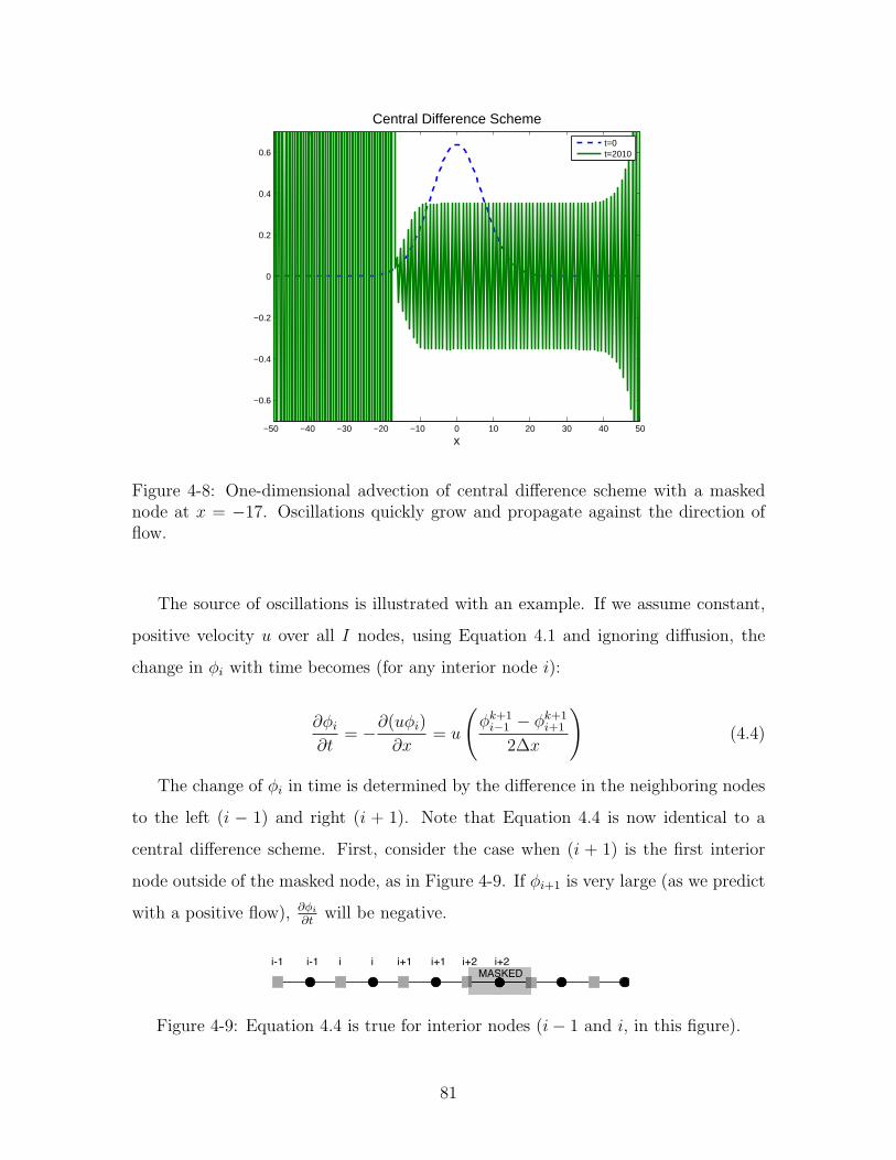
−50 −40 −30 −20 −10 0 10 20 30 40 50
−0.6
−0.4
−0.2
0
0.2
0.4
0.6
Central Difference Scheme
x
t=0t=2010
Figure 4-8: One-dimensional advection of central difference scheme with a maskednode at x = −17. Oscillations quickly grow and propagate against the direction offlow.
The source of oscillations is illustrated with an example. If we assume constant,
positive velocity u over all I nodes, using Equation 4.1 and ignoring diffusion, the
change in φi with time becomes (for any interior node i):
∂φi∂t
= −∂(uφi)
∂x= u
(φk+1i−1 − φk+1
i+1
2∆x
)(4.4)
The change of φi in time is determined by the difference in the neighboring nodes
to the left (i − 1) and right (i + 1). Note that Equation 4.4 is now identical to a
central difference scheme. First, consider the case when (i + 1) is the first interior
node outside of the masked node, as in Figure 4-9. If φi+1 is very large (as we predict
with a positive flow), ∂φi∂t
will be negative.
i-1 i-1 i i i+1 i+1 i+2 i+2
MASKED
Figure 4-9: Equation 4.4 is true for interior nodes (i− 1 and i, in this figure).
81
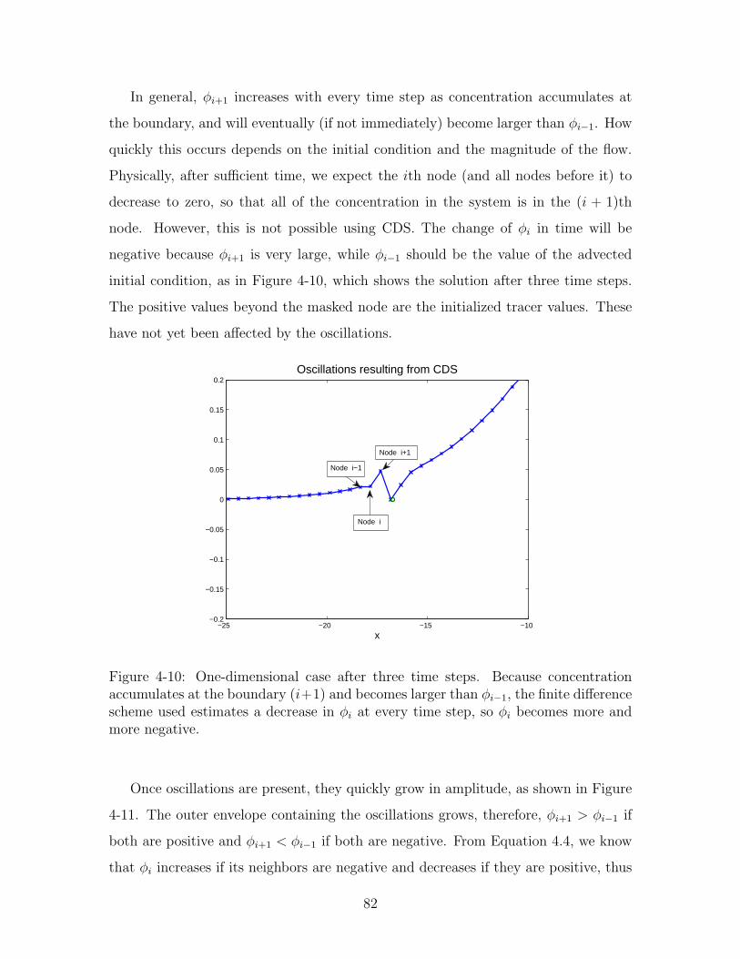
In general, φi+1 increases with every time step as concentration accumulates at
the boundary, and will eventually (if not immediately) become larger than φi−1. How
quickly this occurs depends on the initial condition and the magnitude of the flow.
Physically, after sufficient time, we expect the ith node (and all nodes before it) to
decrease to zero, so that all of the concentration in the system is in the (i + 1)th
node. However, this is not possible using CDS. The change of φi in time will be
negative because φi+1 is very large, while φi−1 should be the value of the advected
initial condition, as in Figure 4-10, which shows the solution after three time steps.
The positive values beyond the masked node are the initialized tracer values. These
have not yet been affected by the oscillations.
−25 −20 −15 −10−0.2
−0.15
−0.1
−0.05
0
0.05
0.1
0.15
0.2Oscillations resulting from CDS
x
Node i−1
Node i
Node i+1
Figure 4-10: One-dimensional case after three time steps. Because concentrationaccumulates at the boundary (i+1) and becomes larger than φi−1, the finite differencescheme used estimates a decrease in φi at every time step, so φi becomes more andmore negative.
Once oscillations are present, they quickly grow in amplitude, as shown in Figure
4-11. The outer envelope containing the oscillations grows, therefore, φi+1 > φi−1 if
both are positive and φi+1 < φi−1 if both are negative. From Equation 4.4, we know
that φi increases if its neighbors are negative and decreases if they are positive, thus
82
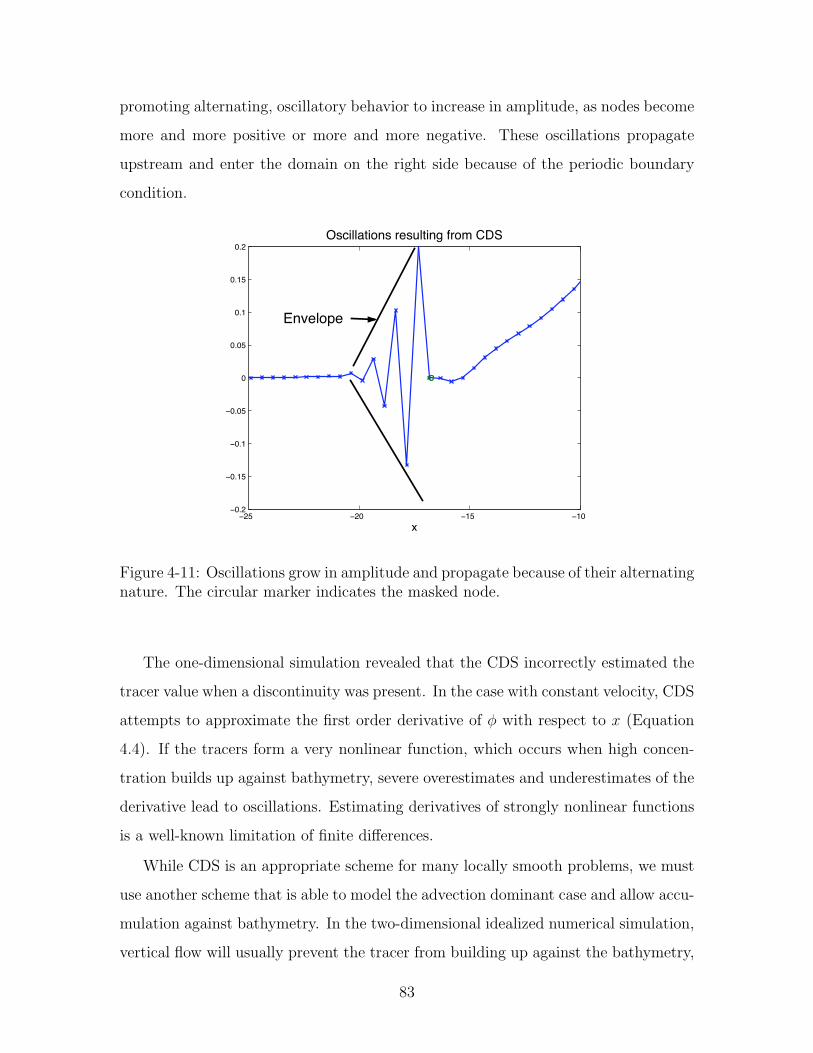
promoting alternating, oscillatory behavior to increase in amplitude, as nodes become
more and more positive or more and more negative. These oscillations propagate
upstream and enter the domain on the right side because of the periodic boundary
condition.
!!" !!# !$" !$#!#%!
!#%$"
!#%$
!#%#"
#
#%#"
#%$
#%$"
#%!
&'()**+,)-.'/01'2*,).3/40-5/678
9
Envelope
Figure 4-11: Oscillations grow in amplitude and propagate because of their alternatingnature. The circular marker indicates the masked node.
The one-dimensional simulation revealed that the CDS incorrectly estimated the
tracer value when a discontinuity was present. In the case with constant velocity, CDS
attempts to approximate the first order derivative of φ with respect to x (Equation
4.4). If the tracers form a very nonlinear function, which occurs when high concen-
tration builds up against bathymetry, severe overestimates and underestimates of the
derivative lead to oscillations. Estimating derivatives of strongly nonlinear functions
is a well-known limitation of finite differences.
While CDS is an appropriate scheme for many locally smooth problems, we must
use another scheme that is able to model the advection dominant case and allow accu-
mulation against bathymetry. In the two-dimensional idealized numerical simulation,
vertical flow will usually prevent the tracer from building up against the bathymetry,
83
so the one-dimensional case presented here can be thought of as a “worst case” sce-
nario. Further, different velocity fields and initial conditions may produce oscillations
much more slowly or may never produce oscillations at all. However, we require a
robust scheme that does not severely limit which physical processes and initial con-
ditions we are able to use.
4.2.3 Donor-Cell Scheme
The donor-cell scheme is a first-order numerical scheme in space, as described by
[23]. This scheme is typically used for terms of the form d(uφ)dx
with u and φ on a
staggered grid, thus it is easily adaptable to our problem setup. For a positive flow, a
derivative at i is estimated by taking the difference of that node with i− 1, the node
in the direction from which the concentration flows. Alternately, the derivative for
a negative flow uses nodes i and i + 1. The donor-cell scheme uses two neighboring
points in its stencil, therefore the oscillations that appeared previously when using the
CDS scheme are not expected to occur. Again, the time discretization is implicit. The
overestimating/underestimating which is severe when a derivative is calculated based
on immediate neighbors will not occur when the value of the ith node is included in
the discretization. This scheme is expressed in Equation 4.5 to represent the advective
term.
∂(uφ)
∂x
∣∣∣∣i
=(φi+1(ui+1 − |ui+1|) + φi(ui+1 + |ui+1| − ui + |ui|) + φi−1(−ui − |ui|))
2∆x
(4.5)
As expected, a simple test of the donor-cell scheme in the two-dimensional domain
did not reveal any oscillations. A one-dimensional test (identical to the test case in
Section 4.2.2) showed that, in fact, all of the concentration advected to the masked
node accumulated without oscillation (Figure 4-13).
Figure 4-14 presents a comparison of the numerical diffusivity and computation
times of the CDS and donor-cell schemes after propagating one cycle (2010 time
84

x
z
N field at timestep=500 using DC
10 20 30 40 50 60 70 80 90 100
10
20
30
40
50
60
70
80
90
100 0
0.5
1
1.5
2
2.5
3
Figure 4-12: Two-dimensional test case using the donor-cell scheme. There are nooscillations, but numerical diffusion is present.
−50 −40 −30 −20 −10 0 10 20 30 40 50
−0.6
−0.4
−0.2
0
0.2
0.4
0.6
Upwind Scheme
x
t=0t=2010
Figure 4-13: One-dimensional advection of donor-cell scheme with a masked node atx = −17. Unlike the case using CDS, the concentration accumulated at the boundarydoes not produce oscillations.
85
steps) in the one-dimensional domain without a masked node. Normalized spread
is used as an indicator of numerical diffusion. After the Gaussian distribution is
propagated, the spread of the distribution is measured at half of the maximum. This
value is normalized by the initial spread measured at half the height of the initial peak.
Therefore, a spread value of one indicates the distribution is perfectly unchanged after
one cycle. Computation time is the averaged time, in seconds, it took to complete
the computations for one cycle using MATLAB 7.4.0. Graphs shown are qualitatively
informative: computational time on different machines or programs are likely to give
different results, but the comparison between the two schemes remains qualitatively
valid. Several different grid resolutions (from 15 to 400 nodes) give a range of spread
and computation times.
For the spread versus computational time graph, we look for the scheme that has
both low spread and low computational time. From Figure 4-14, we see that CDS out-
performs the donor-cell scheme for all but very low resolutions. After computational
times above ten seconds, the spread does not continue to decrease, but instead levels
to just above one. The donor-cell scheme is diffusive, even for very high resolution
grids.
For the donor-cell scheme, oscillations could not propagate because there is enough
numerical diffusion in the system to smooth large negative and positive values before
they are able to grow and spread. The CDS is much less diffusive, but is oscillatory.
An ideal scheme would combine the avoidance of oscillations of the donor-cell scheme
and the low numerical diffusivity of CDS. Therefore, the next numerical scheme we
examined is a hybrid scheme, which is a weighted combination of donor-cell and CDS.
4.2.4 Hybrid Scheme
The hybrid scheme offers a weighted combination of CDS and donor-cell. The donor-
cell and CDS are combined according to a weight γ: (1−γ)(D-C) +γ CDS, where D-C
is the result from the donor-cell scheme. A very low value of γ is close to first-order
accuracy, like the donor-cell scheme, while a value near unity is closer to second-order
accurate, like the CDS.
86
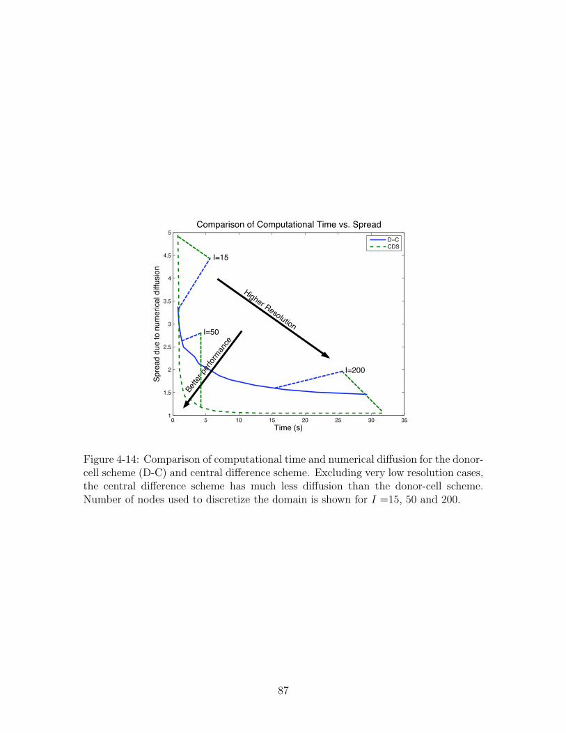
! " #! #" $! $" %! %"#
#&"
$
$&"
%
%&"
'
'&"
"
()*+,-./
012+34,45+,67,85*+2)93:,4);;5.)78
<7*132).78,7;,<7*15636)783:,()*+,=.&,012+34
,
,
>!<
<>0
Better performance
Higher Resolution
I=15
I=50
I=200
Figure 4-14: Comparison of computational time and numerical diffusion for the donor-cell scheme (D-C) and central difference scheme. Excluding very low resolution cases,the central difference scheme has much less diffusion than the donor-cell scheme.Number of nodes used to discretize the domain is shown for I =15, 50 and 200.
87

Applying the hybrid scheme to the two-dimensional test case (Figure 4-15) reveals
oscillations for higher γ values, which disappear for lower γ values. We are effectively
introducing numerical diffusion by decreasing γ and for some critical value, there
is enough diffusion to average the oscillations quickly enough so that they do not
grow and propagate, as with the CDS case. This critical value depends on the local
gradient of concentration, the rate of advection and the grid resolution.
x
z
N field at timestep=500 using hybrid scheme
10 20 30 40 50 60 70 80 90 100
10
20
30
40
50
60
70
80
90
100 0
0.5
1
1.5
2
2.5
3
Figure 4-15: Two-dimension test case using γ = 0.5 is absent of oscillations and lessdiffusive than the donor-cell scheme.
By examining various γ values (0.75, 0.5, and 0.25) in the one-dimensional test
case, it is clear that lower values of γ produce oscillations with smaller amplitudes
that propagate more slowly, or do not propagate after a certain distance. Figures 4-
16(a) – 4-16(c)) show Gaussian distributions advected over the same number of time
steps with identical speeds and masked nodes. While all three values of γ produce
oscillations, it is less severe for smaller values of γ. Still, for even very small γ (0.005),
small oscillatory behavior can be seen (Figure 4-16(d)). Therefore, using the hybrid
scheme does not give us the non-oscillatory, non-diffusive results we desire.
88
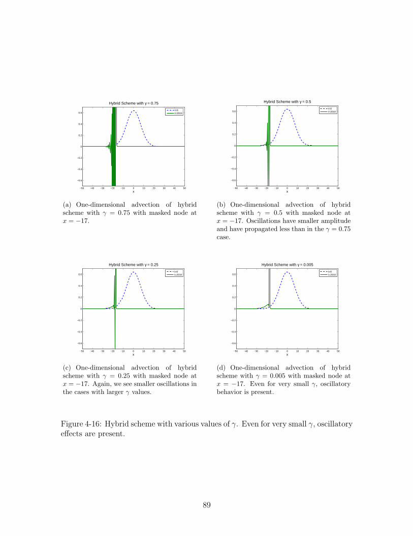
−50 −40 −30 −20 −10 0 10 20 30 40 50
−0.6
−0.4
−0.2
0
0.2
0.4
0.6
Hybrid Scheme with γ = 0.75
x
t=0t=2010
(a) One-dimensional advection of hybridscheme with γ = 0.75 with masked node atx = −17.
−50 −40 −30 −20 −10 0 10 20 30 40 50
−0.6
−0.4
−0.2
0
0.2
0.4
0.6
Hybrid Scheme with γ = 0.5
x
t=0t=2010
(b) One-dimensional advection of hybridscheme with γ = 0.5 with masked node atx = −17. Oscillations have smaller amplitudeand have propagated less than in the γ = 0.75case.
−50 −40 −30 −20 −10 0 10 20 30 40 50
−0.6
−0.4
−0.2
0
0.2
0.4
0.6
Hybrid Scheme with γ = 0.25
x
t=0t=2010
(c) One-dimensional advection of hybridscheme with γ = 0.25 with masked node atx = −17. Again, we see smaller oscillations inthe cases with larger γ values.
−50 −40 −30 −20 −10 0 10 20 30 40 50
−0.6
−0.4
−0.2
0
0.2
0.4
0.6
Hybrid Scheme with γ = 0.005
x
t=0t=2010
(d) One-dimensional advection of hybridscheme with γ = 0.005 with masked node atx = −17. Even for very small γ, oscillatorybehavior is present.
Figure 4-16: Hybrid scheme with various values of γ. Even for very small γ, oscillatoryeffects are present.
89
4.2.5 Weighted Essentially Non-Oscillatory (WENO) Scheme
The WENO scheme ([51]) is a higher-order accurate finite difference or finite vol-
ume scheme specifically created for problems (often in computational fluid dynamics)
which contain piecewise smooth solutions with discontinuities. While the discretized
equation is linear, a nonlinear adaptive procedure is used to avoid discontinuities in
the interpolation process by choosing the smoothest stencil locally. WENO chooses
a convex combination of all possible stencils, instead of using the single smoothest
stencil (as is the case with the Essentially Non-Oscillatory (ENO) scheme [28]). These
schemes have been particularly successful in many problems, especially those contain-
ing shocks or compressible turbulence simulations [51], but this scheme has not yet
been applied to coupled physics-biology modeling.
Because masking is used in the numerical simulation for idealized physics and bi-
ology, there are zero velocity values and fixed tracer values under this mask. Outside
of the bathymetry, however, there are nonzero and changing values, especially for
nutrients, which dominate in deep water. Therefore, a sharp discontinuity is present
at the boundary of the bathymetry and the previously used finite difference meth-
ods unsuccessfully attempt to estimate the derivative of a nonlinear function using
conventional methods.
To avoid numerical diffusion, a finer mesh or higher-order scheme is necessary.
However, we are limited to the mesh size due to computational cost, and higher order
schemes introduce oscillations near a discontinuity, which do not decay in magnitude
when the mesh is refined. Prior to the WENO scheme, many people used explicit
artificial viscosity or limiters to eliminate or reduce such oscillations. However, artifi-
cial viscosity depends on fine tuning the individual problem at the discontinuity and
the limiters force accuracy to become first order near all extrema, including smooth
extrema. In addition, limiters are not self-similar (mesh size dependent parameter
exists) [51].
The order of accuracy for the WENO scheme is determined by the number of
stencils, and number of points in those stencils. As shown in Figure 4-17, we use
90
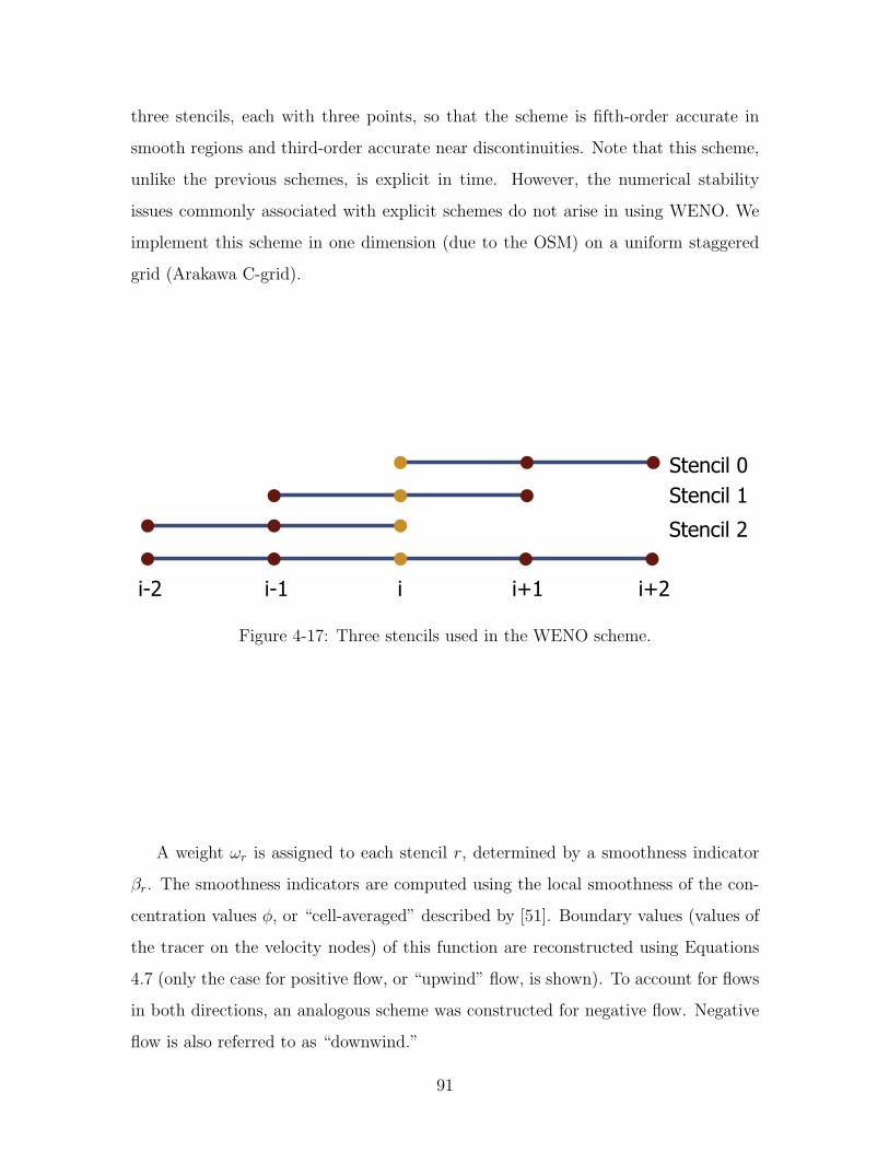
three stencils, each with three points, so that the scheme is fifth-order accurate in
smooth regions and third-order accurate near discontinuities. Note that this scheme,
unlike the previous schemes, is explicit in time. However, the numerical stability
issues commonly associated with explicit schemes do not arise in using WENO. We
implement this scheme in one dimension (due to the OSM) on a uniform staggered
grid (Arakawa C-grid).
i-2 i-1 i i+1 i+2
Stencil 0
Stencil 1
Stencil 2
Figure 4-17: Three stencils used in the WENO scheme.
A weight ωr is assigned to each stencil r, determined by a smoothness indicator
βr. The smoothness indicators are computed using the local smoothness of the con-
centration values φ, or “cell-averaged” described by [51]. Boundary values (values of
the tracer on the velocity nodes) of this function are reconstructed using Equations
4.7 (only the case for positive flow, or “upwind” flow, is shown). To account for flows
in both directions, an analogous scheme was constructed for negative flow. Negative
flow is also referred to as “downwind.”
91

ωr =αr∑2s=0 αs
for r = 0, 1, 2
where
αr =dr
(ε+ βr)2
d0 =3
10, d1 =
3
5, d2 =
1
10
β0 =13
12(φi − 2φi+1 + φi+2)
2 +1
4(3φi − 4φi+1 + φi+2)
2
β1 =13
12(φi−1 − 2φi + φi+1)
2 +1
4(φi−1 − φi+1)
2
β2 =13
12(φi−2 − 2φi−1 + φi)
2 +1
4(φi−2 − 4φi−1 + 3φi)
2
(4.6)
where ε = 10−6 to avoid a zero denominator, ωr ≥ 0 and∑
r ωr = 1 for stability
and consistency, and dr is always positive and∑
r dr = 1 for consistency. When
a discontinuity is encountered, the weights associated with the stencils that cross
that discontinuity become nearly zero so that only stencils that do not cross the
discontinuity are used.
φi =1
3φi−2 −
7
6φi−1 +
11
6φi
φi+1 = −1
6φi−1 +
5
6φi +
1
3φi+1
φi+2 =1
3φi +
5
6φi+1 −
1
6φi+2
(4.7)
where φ values are tracers values on velocity nodes and φ are tracer values on tracer
nodes. The weighted combinations give a new approximation to the tracer value on
the velocity node, φ∗.
92
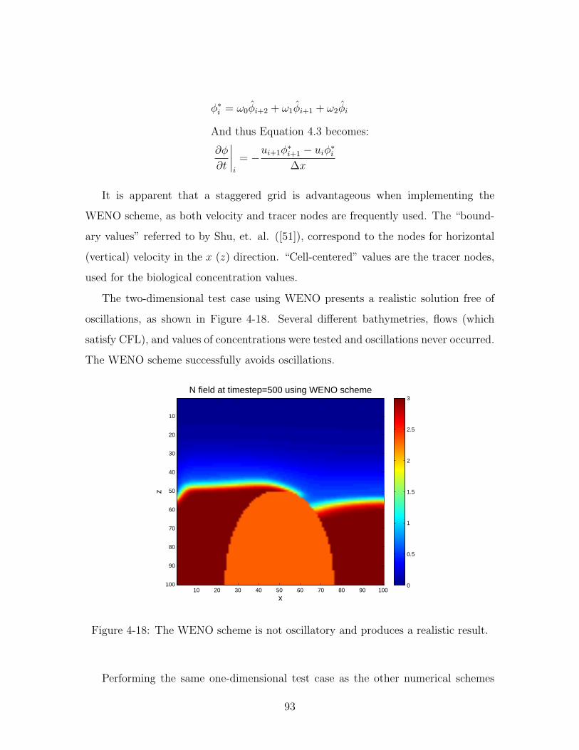
φ∗i = ω0φi+2 + ω1φi+1 + ω2φi
And thus Equation 4.3 becomes:
∂φ
∂t
∣∣∣∣i
= −ui+1φ
∗i+1 − uiφ∗i∆x
It is apparent that a staggered grid is advantageous when implementing the
WENO scheme, as both velocity and tracer nodes are frequently used. The “bound-
ary values” referred to by Shu, et. al. ([51]), correspond to the nodes for horizontal
(vertical) velocity in the x (z) direction. “Cell-centered” values are the tracer nodes,
used for the biological concentration values.
The two-dimensional test case using WENO presents a realistic solution free of
oscillations, as shown in Figure 4-18. Several different bathymetries, flows (which
satisfy CFL), and values of concentrations were tested and oscillations never occurred.
The WENO scheme successfully avoids oscillations.
x
z
N field at timestep=500 using WENO scheme
10 20 30 40 50 60 70 80 90 100
10
20
30
40
50
60
70
80
90
100 0
0.5
1
1.5
2
2.5
3
Figure 4-18: The WENO scheme is not oscillatory and produces a realistic result.
Performing the same one-dimensional test case as the other numerical schemes
93
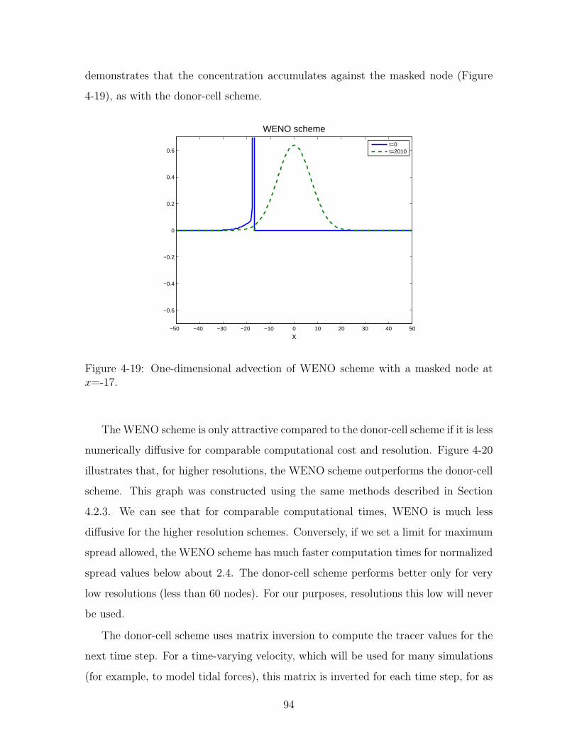
demonstrates that the concentration accumulates against the masked node (Figure
4-19), as with the donor-cell scheme.
−50 −40 −30 −20 −10 0 10 20 30 40 50
−0.6
−0.4
−0.2
0
0.2
0.4
0.6
x
WENO scheme
t=0t=2010
Figure 4-19: One-dimensional advection of WENO scheme with a masked node atx=-17.
The WENO scheme is only attractive compared to the donor-cell scheme if it is less
numerically diffusive for comparable computational cost and resolution. Figure 4-20
illustrates that, for higher resolutions, the WENO scheme outperforms the donor-cell
scheme. This graph was constructed using the same methods described in Section
4.2.3. We can see that for comparable computational times, WENO is much less
diffusive for the higher resolution schemes. Conversely, if we set a limit for maximum
spread allowed, the WENO scheme has much faster computation times for normalized
spread values below about 2.4. The donor-cell scheme performs better only for very
low resolutions (less than 60 nodes). For our purposes, resolutions this low will never
be used.
The donor-cell scheme uses matrix inversion to compute the tracer values for the
next time step. For a time-varying velocity, which will be used for many simulations
(for example, to model tidal forces), this matrix is inverted for each time step, for as
94
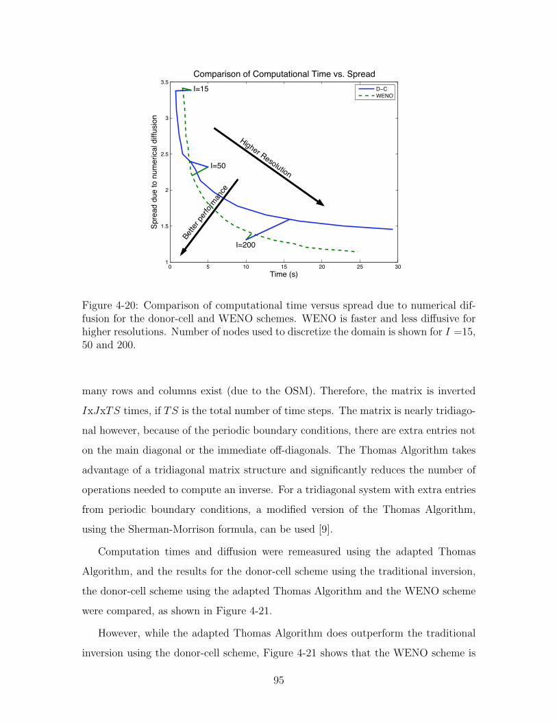
! " #! #" $! $" %!#
#&"
$
$&"
%
%&"
'()*+,-.
/01*23+34*+56+74)*1(829+3(::4-(67
;6)021(-67+6:+;6)04525(6729+'()*+<-&+/01*23
+
+
=!;
>?@A
Better performance
Higher Resolution
I=15
I=50
I=200
Figure 4-20: Comparison of computational time versus spread due to numerical dif-fusion for the donor-cell and WENO schemes. WENO is faster and less diffusive forhigher resolutions. Number of nodes used to discretize the domain is shown for I =15,50 and 200.
many rows and columns exist (due to the OSM). Therefore, the matrix is inverted
IxJxTS times, if TS is the total number of time steps. The matrix is nearly tridiago-
nal however, because of the periodic boundary conditions, there are extra entries not
on the main diagonal or the immediate off-diagonals. The Thomas Algorithm takes
advantage of a tridiagonal matrix structure and significantly reduces the number of
operations needed to compute an inverse. For a tridiagonal system with extra entries
from periodic boundary conditions, a modified version of the Thomas Algorithm,
using the Sherman-Morrison formula, can be used [9].
Computation times and diffusion were remeasured using the adapted Thomas
Algorithm, and the results for the donor-cell scheme using the traditional inversion,
the donor-cell scheme using the adapted Thomas Algorithm and the WENO scheme
were compared, as shown in Figure 4-21.
However, while the adapted Thomas Algorithm does outperform the traditional
inversion using the donor-cell scheme, Figure 4-21 shows that the WENO scheme is
95
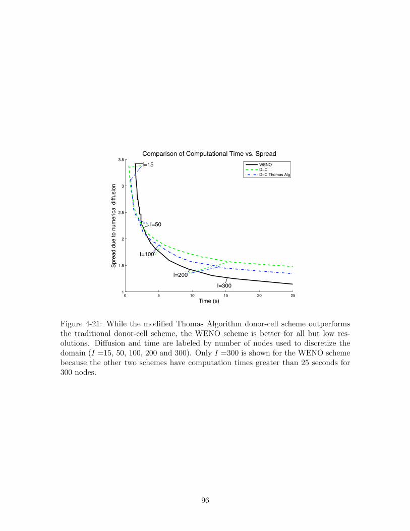
! " #! #" $! $"#
#%"
$
$%"
&
&%"
'()*+,-,.*-/0-1.2*)34+5-,366.7301
832*-97:
;02(+)3701-06-;02(./+/301+5-832*-<7%-'()*+,
-
-
=>?@
A!;
A!;-8B02+7-C5D
I=15
I=50
I=100
I=200
I=300
Figure 4-21: While the modified Thomas Algorithm donor-cell scheme outperformsthe traditional donor-cell scheme, the WENO scheme is better for all but low res-olutions. Diffusion and time are labeled by number of nodes used to discretize thedomain (I =15, 50, 100, 200 and 300). Only I =300 is shown for the WENO schemebecause the other two schemes have computation times greater than 25 seconds for300 nodes.
96
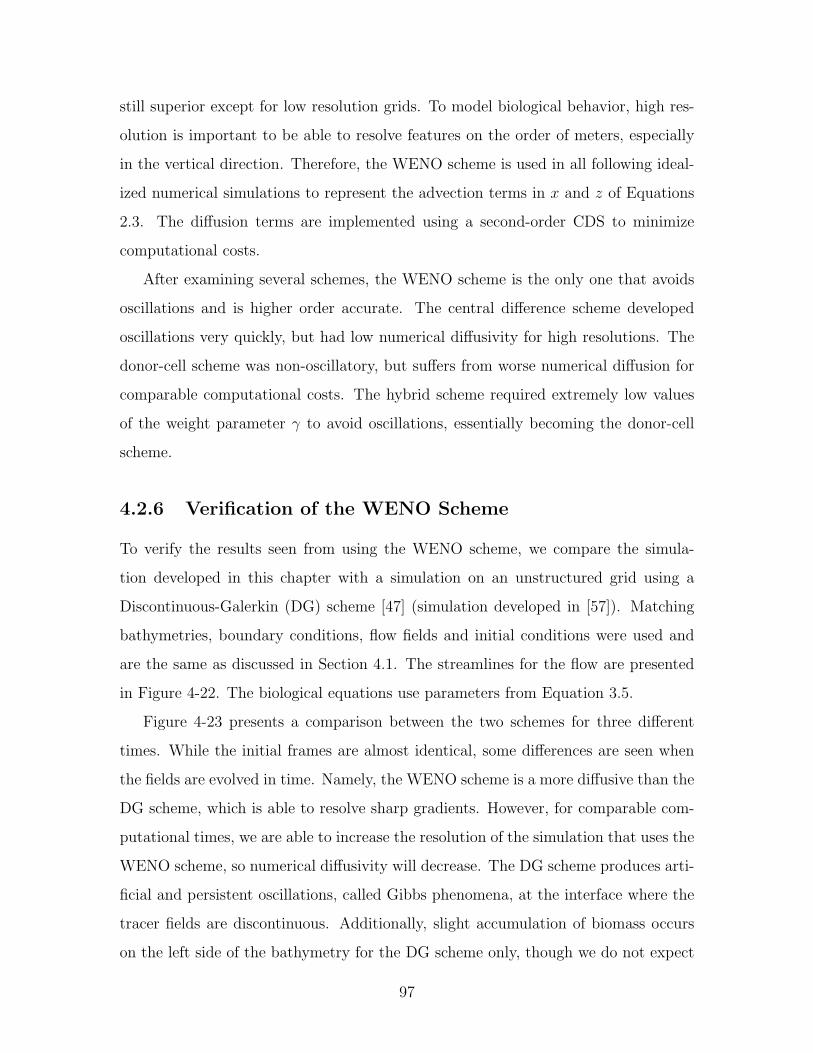
still superior except for low resolution grids. To model biological behavior, high res-
olution is important to be able to resolve features on the order of meters, especially
in the vertical direction. Therefore, the WENO scheme is used in all following ideal-
ized numerical simulations to represent the advection terms in x and z of Equations
2.3. The diffusion terms are implemented using a second-order CDS to minimize
computational costs.
After examining several schemes, the WENO scheme is the only one that avoids
oscillations and is higher order accurate. The central difference scheme developed
oscillations very quickly, but had low numerical diffusivity for high resolutions. The
donor-cell scheme was non-oscillatory, but suffers from worse numerical diffusion for
comparable computational costs. The hybrid scheme required extremely low values
of the weight parameter γ to avoid oscillations, essentially becoming the donor-cell
scheme.
4.2.6 Verification of the WENO Scheme
To verify the results seen from using the WENO scheme, we compare the simula-
tion developed in this chapter with a simulation on an unstructured grid using a
Discontinuous-Galerkin (DG) scheme [47] (simulation developed in [57]). Matching
bathymetries, boundary conditions, flow fields and initial conditions were used and
are the same as discussed in Section 4.1. The streamlines for the flow are presented
in Figure 4-22. The biological equations use parameters from Equation 3.5.
Figure 4-23 presents a comparison between the two schemes for three different
times. While the initial frames are almost identical, some differences are seen when
the fields are evolved in time. Namely, the WENO scheme is a more diffusive than the
DG scheme, which is able to resolve sharp gradients. However, for comparable com-
putational times, we are able to increase the resolution of the simulation that uses the
WENO scheme, so numerical diffusivity will decrease. The DG scheme produces arti-
ficial and persistent oscillations, called Gibbs phenomena, at the interface where the
tracer fields are discontinuous. Additionally, slight accumulation of biomass occurs
on the left side of the bathymetry for the DG scheme only, though we do not expect
97
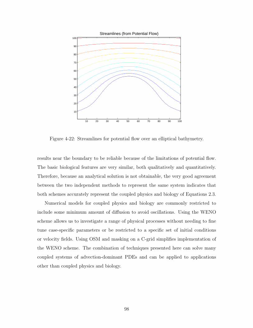
Streamlines (from Potential Flow)
10 20 30 40 50 60 70 80 90 100
10
20
30
40
50
60
70
80
90
100
Figure 4-22: Streamlines for potential flow over an elliptical bathymetry.
results near the boundary to be reliable because of the limitations of potential flow.
The basic biological features are very similar, both qualitatively and quantitatively.
Therefore, because an analytical solution is not obtainable, the very good agreement
between the two independent methods to represent the same system indicates that
both schemes accurately represent the coupled physics and biology of Equations 2.3.
Numerical models for coupled physics and biology are commonly restricted to
include some minimum amount of diffusion to avoid oscillations. Using the WENO
scheme allows us to investigate a range of physical processes without needing to fine
tune case-specific parameters or be restricted to a specific set of initial conditions
or velocity fields. Using OSM and masking on a C-grid simplifies implementation of
the WENO scheme. The combination of techniques presented here can solve many
coupled systems of advection-dominant PDEs and can be applied to applications
other than coupled physics and biology.
98
(a) Simulation using WENO scheme at t=0days.
(b) Simulation using DG scheme at t=0 days.
(c) Simulation using WENO scheme at t=30days.
(d) Simulation using DG scheme at t=30 days.
(e) Simulation using WENO scheme at t=50days.
(f) Simulation using DG scheme at t=50 days.
Figure 4-23: Comparison between simulations using the WENO scheme andDiscontinuous-Galerkin [57].
99

100

Chapter 5
Physical-Biological Interactions
with Tides in the San Bernardino
Strait
In this chapter, we compare two- and three-dimensional realistic simulations of the
interaction between tides and biology in the San Bernardino Strait. Tides can produce
strong mixing in coastal waters, create internal waves over bathymetry, and suspend
bottom sediment. Such mixing can create interesting biological features, even in two
dimensions. Thus we will focus on the relationship between tides and biology as an
example of the range of features that our two-dimensional idealized simulation is able
to represent. Tidal frequencies range from semi-diurnal to diurnal to even longer
periods. We will consider a range of tidal frequencies, but will focus on periods less
than one month. A more detailed discussion of tides can be found in [54].
Similar cases are initialized in both two and three dimensions with bathymetry
and initial conditions motivated by San Bernardino Strait. For the two-dimensional
case, details of the bathymetry, velocity field, initial conditions, boundary conditions
and parameters are discussed in Section 5.1. Cases with different tidal frequencies,
parameters and levels of diffusion are examined and compared.
The three-dimensional case is simulated in MSEAS. Details of initialization, flow
fields, bathymetry and parameters are discussed in Section 5.2. We present a new
101
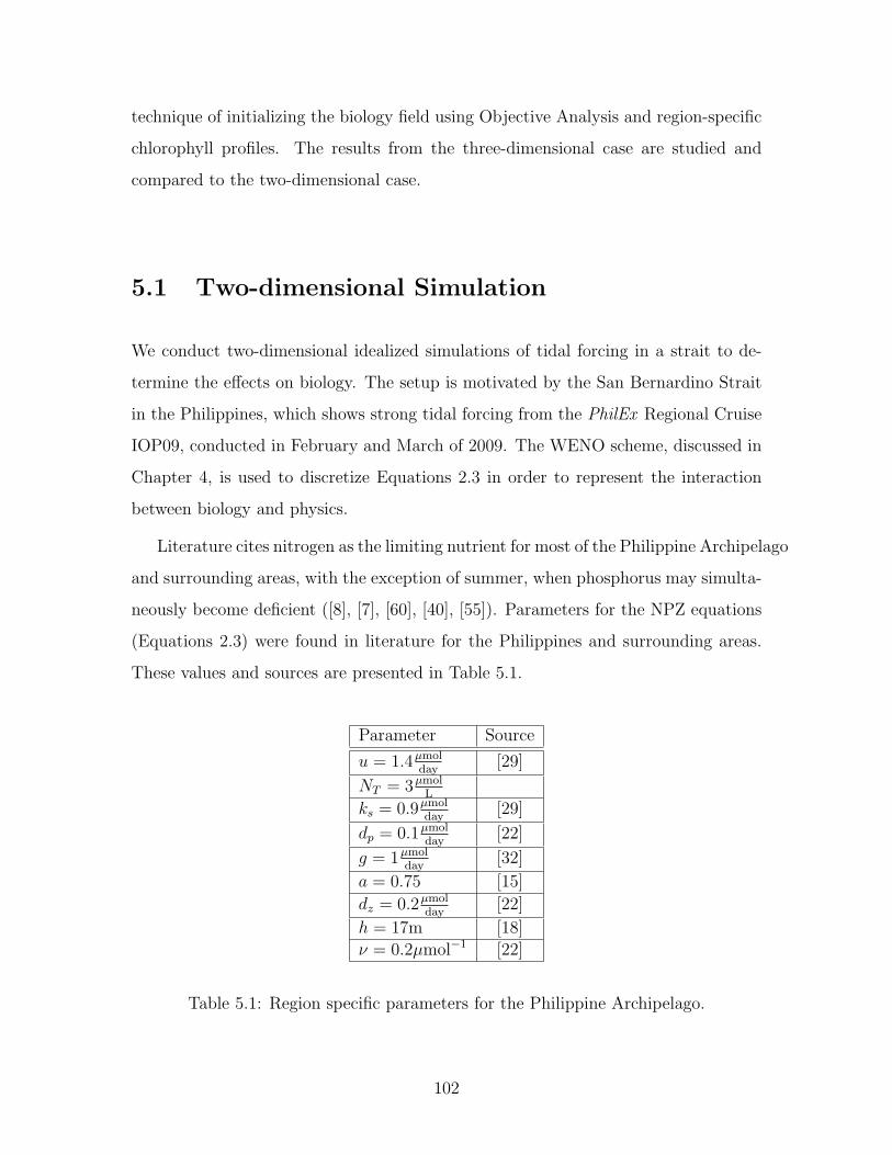
technique of initializing the biology field using Objective Analysis and region-specific
chlorophyll profiles. The results from the three-dimensional case are studied and
compared to the two-dimensional case.
5.1 Two-dimensional Simulation
We conduct two-dimensional idealized simulations of tidal forcing in a strait to de-
termine the effects on biology. The setup is motivated by the San Bernardino Strait
in the Philippines, which shows strong tidal forcing from the PhilEx Regional Cruise
IOP09, conducted in February and March of 2009. The WENO scheme, discussed in
Chapter 4, is used to discretize Equations 2.3 in order to represent the interaction
between biology and physics.
Literature cites nitrogen as the limiting nutrient for most of the Philippine Archipelago
and surrounding areas, with the exception of summer, when phosphorus may simulta-
neously become deficient ([8], [7], [60], [40], [55]). Parameters for the NPZ equations
(Equations 2.3) were found in literature for the Philippines and surrounding areas.
These values and sources are presented in Table 5.1.
Parameter Source
u = 1.4µmolday
[29]
NT = 3µmolL
ks = 0.9µmolday
[29]
dp = 0.1µmolday
[22]
g = 1µmolday
[32]
a = 0.75 [15]
dz = 0.2µmolday
[22]
h = 17m [18]
ν = 0.2µmol−1 [22]
Table 5.1: Region specific parameters for the Philippine Archipelago.
102

5.1.1 Bathymetry
For the bathymetry used in the two-dimensional case, we developed an algorithm
to find the deepest path through the San Bernardino Strait using data with one-
minute resolution from Smith and Sandwell (v.10.1) [53] in the domain 124oE−125oE
and 12oN−13.1oN (Figure 5-1). The algorithm uses a modified Dijkstra’s algorithm
[14], also known as the “shortest path algorithm,” altered by recording the depth at
each point instead of the distance between two points. The algorithm begins on the
southern border of the domain and marches northward row by row. As described,
the algorithm will provide a collection of deepest points that are not in any sense
connected to form a path. To introduce the notion of a path, we imposed a limiter so
that points selected in adjacent rows are restricted to be at most one column apart;
the path is restricted to moving to a neighboring node (either one node north, one
node northeast, or one node northwest). The sum of depths is recorded for each
path; this is our metric for determining the “deepest path” through the strait. As
the algorithm marches northward, only the sums and paths for the deepest paths are
kept at each stage, as the deepest path for any new path starting from the current
row would use the paths already recorded for an overall optimal path. The algorithm
ends at the northern border of the domain, where the node on that row with the
largest negative summed depths is selected as the deepest path. We then find the
bathymetry associated with this deepest path. Finally, we apply a Gaussian low pass
filter to the resulting bathymetry of the deepest path and record the depth profile,
using the smoothed bathymetry along the deepest path. This bathymetry, with flat
bathymetry added on each side for reasons discussed in Section 5.1.3, is shown in
Figure 5-2.
5.1.2 Velocity Field
We assume the flow is inviscid and irrotational and that the strait is narrow enough
so that rotational effects can be ignored (this is true if the ratio of the channel width
to the Rossby radius is small [52], [45], [13]). For the San Bernardino Strait, the
103
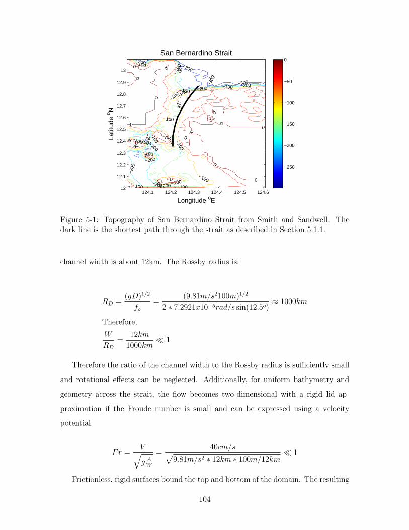
−300−300
−300
−200
−200
−200
−200−200
−200
−200
−200
−200
−200
−200
−100 −100
−100
−100−100
−100
−100
−100−100
−100−100
−100
−100
−100
−100
−100
−100
−100
0000
0
0
0
00
0
0
0
00
0
0
0
0
00
0
00
Longitude oE
Latit
ude
o N
San Bernardino Strait
124.1 124.2 124.3 124.4 124.5 124.612
12.1
12.2
12.3
12.4
12.5
12.6
12.7
12.8
12.9
13
−250
−200
−150
−100
−50
0
Figure 5-1: Topography of San Bernardino Strait from Smith and Sandwell. Thedark line is the shortest path through the strait as described in Section 5.1.1.
channel width is about 12km. The Rossby radius is:
RD =(gD)1/2
fo=
(9.81m/s2100m)1/2
2 ∗ 7.2921x10−5rad/s sin(12.5o)≈ 1000km
Therefore,
W
RD
=12km
1000km� 1
Therefore the ratio of the channel width to the Rossby radius is sufficiently small
and rotational effects can be neglected. Additionally, for uniform bathymetry and
geometry across the strait, the flow becomes two-dimensional with a rigid lid ap-
proximation if the Froude number is small and can be expressed using a velocity
potential.
Fr =V√g AW
=40cm/s√
9.81m/s2 ∗ 12km ∗ 100m/12km� 1
Frictionless, rigid surfaces bound the top and bottom of the domain. The resulting
104

Figure 5-2: Bathymetry and initial condition for the two-dimensional simulations ofthe San Bernardino Strait.
105

governing equation is the Laplacian of the velocity potential. A similar setup was used
by Signell [52] for tidal flow over elliptic and Gaussian-shaped coastal headlands, using
the vertically averaged velocity for dynamics in the horizontal plane instead. The flow
field resulting from this method does not accurately model flow at the bathymetry
boundary because we assume frictionless flow. For boundary conditions, we assume
no flow through the ocean bottom or air-sea interface and unit velocity at the side
boundaries, which may be scaled later. The resulting streamlines are shown in Figure
5-3.
Streamlines for Potential Flow
50 100 150 200 250 300
50
100
150
200
250
300
Figure 5-3: Streamlines of the potential flow resulting from the bathymetry of theSan Bernardino Strait.
We studied generalized inverse high-resolution data on barotropic tides [38] to
determine the magnitude and frequency of oscillation with which to force our flow.
For the months of February and March, a maximum velocity of about 100 cm/s
is observed for most days. Two different tidal frequencies are observed: for events
with stronger flow, velocity changes direction four times in one day (semidiurnal),
otherwise it changes twice in a day (diurnal). Dominant tidal constituents in the
San Bernardino Strait, in order of significance, are M2, S2, K1, and O1 [38], so
the semidiurnal constituents (M2 and S2) are dominant, followed by the diurnal
constituents (K1 and O1). We will incorporate this into our model by examining
106
both cases and comparing them against an identical case without oscillating flow.
5.1.3 Biology Initialization
The biology fields were initialized using the equilibrium solution of the steady state
equations without flow (Equations 3.4). We used parameter values found from the
literature (see Table 5.1) which predict stable solutions (using the methods in Chapter
3). Periodic boundary conditions are imposed in the x-direction. We are able to
implement a periodic boundary condition by extending the domain in the x-direction
so that the problem becomes semi-infinite and the biology which leaves one side never
re-enters the portion of the domain we are interested in (that is, over the bathymetry).
The field far from the bathymetry (in the x-direction) is present only to create a
semi-infinite domain and should not influence the dynamics over or around the strait
bathymetry.
5.1.4 Cases
Four different oscillation frequencies were examined in test cases, with two frequen-
cies corresponding to the semidiurnal and diurnal tidal constituents observed for this
strait, one zero frequency case for comparison and a much lower frequency corre-
sponding to the longer period tidal constituent. Cases with and without diffusion are
compared. Additionally, different sets of parameters are examined. The twelve cases
are summarized in Table 5.2.
5.1.5 Comparison of Time Scales
Using different parameter sets and oscillation frequencies leads to several different
time scales. Biological interaction is more active if the time scale of the flow is longer
than the time scale of the biological reaction terms. If the state variables that are
at equilibrium at one depth level are moved vertically by the flow, a longer physical
time scale provides the biology sufficient time to interact completely and adjust to
the new depth level. Examining the terms of Equation 2.3, several time scales result
107
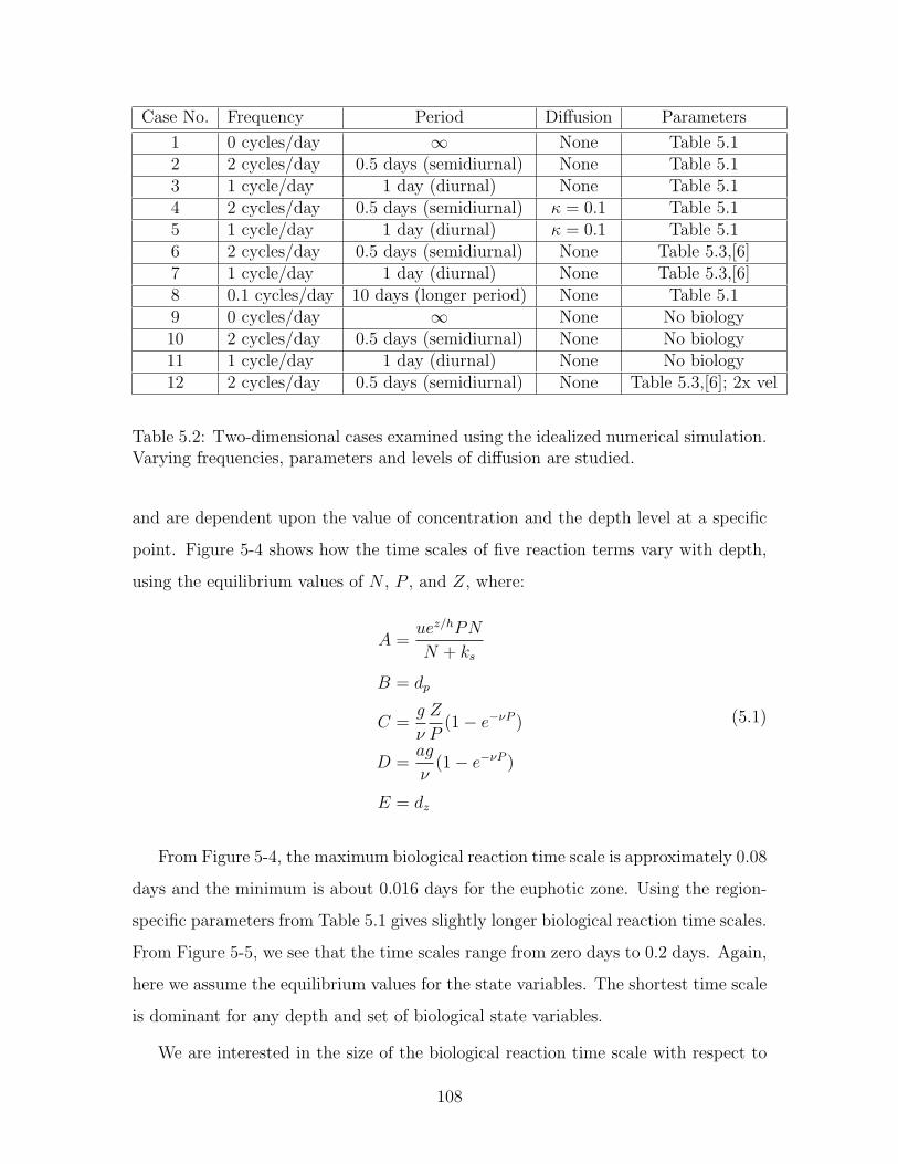
Case No. Frequency Period Diffusion Parameters
1 0 cycles/day ∞ None Table 5.12 2 cycles/day 0.5 days (semidiurnal) None Table 5.13 1 cycle/day 1 day (diurnal) None Table 5.14 2 cycles/day 0.5 days (semidiurnal) κ = 0.1 Table 5.15 1 cycle/day 1 day (diurnal) κ = 0.1 Table 5.16 2 cycles/day 0.5 days (semidiurnal) None Table 5.3,[6]7 1 cycle/day 1 day (diurnal) None Table 5.3,[6]8 0.1 cycles/day 10 days (longer period) None Table 5.19 0 cycles/day ∞ None No biology10 2 cycles/day 0.5 days (semidiurnal) None No biology11 1 cycle/day 1 day (diurnal) None No biology12 2 cycles/day 0.5 days (semidiurnal) None Table 5.3,[6]; 2x vel
Table 5.2: Two-dimensional cases examined using the idealized numerical simulation.Varying frequencies, parameters and levels of diffusion are studied.
and are dependent upon the value of concentration and the depth level at a specific
point. Figure 5-4 shows how the time scales of five reaction terms vary with depth,
using the equilibrium values of N , P , and Z, where:
A =uez/hPN
N + ks
B = dp
C =g
ν
Z
P(1− e−νP )
D =ag
ν(1− e−νP )
E = dz
(5.1)
From Figure 5-4, the maximum biological reaction time scale is approximately 0.08
days and the minimum is about 0.016 days for the euphotic zone. Using the region-
specific parameters from Table 5.1 gives slightly longer biological reaction time scales.
From Figure 5-5, we see that the time scales range from zero days to 0.2 days. Again,
here we assume the equilibrium values for the state variables. The shortest time scale
is dominant for any depth and set of biological state variables.
We are interested in the size of the biological reaction time scale with respect to
108

−0.01 0 0.01 0.02 0.03 0.04 0.05 0.06 0.07 0.08 0.09−100
−90
−80
−70
−60
−50
−40
−30
−20
−10
0
Time (days)
Dep
th (
m)
Time Scales of Biological Reaction TermsUsing Parameter Set From "The Sea"
ABCDE
Figure 5-4: Time scales for the biological reaction terms of Equation 2.3 using pa-rameters from Equation 3.5. These time scales vary in depth and with respect toconcentration of biological variables.
0 0.05 0.1 0.15 0.2 0.25−100
−90
−80
−70
−60
−50
−40
−30
−20
−10
0
Time (days)
Dep
th (
m)
Time Scales of Biological Reaction TermsUsing Region−Specific Parameters
ABCDE
Figure 5-5: Time scales for the biological reaction terms of Equation 2.3 using region-specific parameters from Table 5.1. This set of parameters leads to slightly longertime scales than the previous set of parameters.
109
the physical time scale of the system. The physical time scale is either the period
of oscillation (listed in Table 5.2) or the time it takes for a parcel of fluid to advect
over the bathymetry (about four days), whichever is shorter. The physical time
scale should be greater than the biological reaction time scale for the biological state
variables to be affected by the changing depth levels. Because the biology fields are
initialized using the equilibrium values, the state variables will only change if they
move vertically. If they are transported too quickly and then returned to the initial
depth level, very little biological activity will occur. Comparing our time scales, we
see that the physical time scale is longer than the biological reaction time scale for all
frequencies. Slower oscillations have longer time scales, so we expect more biological
activity for longer tidal periods.
5.1.6 Results
From Case 1, we see in Figure 5-6 that non-oscillatory flow creates increased biological
activity (namely a bloom in phytoplankton) because of the vertical velocities resulting
from the topography. This bloom forms in the first few days and then continues to
advect around because of the periodic boundary conditions, until a system equilibrium
is reached. Compared to Case 9 (Figure 5-14), the case without biological reaction,
the phytoplankton bloom is apparent in the top 50 meters.
For Cases 2 and 3 (Figures 5-7 and 5-8), the oscillations are too fast to allow
sufficient vertical transport for nutrient-rich water to reach shallower depths. Cases
10 and 11 (Figures 5-15 and 5-16), the comparable cases without biological reaction,
actually show a more gradual gradient in depth (most noticeably in the phytoplankton
field above the bathymetry). The sharper gradient is maintained in the cases with
biological reaction (in Cases 2 and 3) because the state variables attempt to move back
to their steady equilibria (discussed in Chapter 3). For example, in Case 2, as high
concentrations of phytoplankton travel deeper, they die quickly because of the lack
of light. However, in Case 10, the tracer simply travels deeper. While the oscillations
are too fast in Cases 2 and 3 to allow biology to react, the system does adjust for the
bathymetry, as we can see with the evolution in time right above the bathymetry in
110
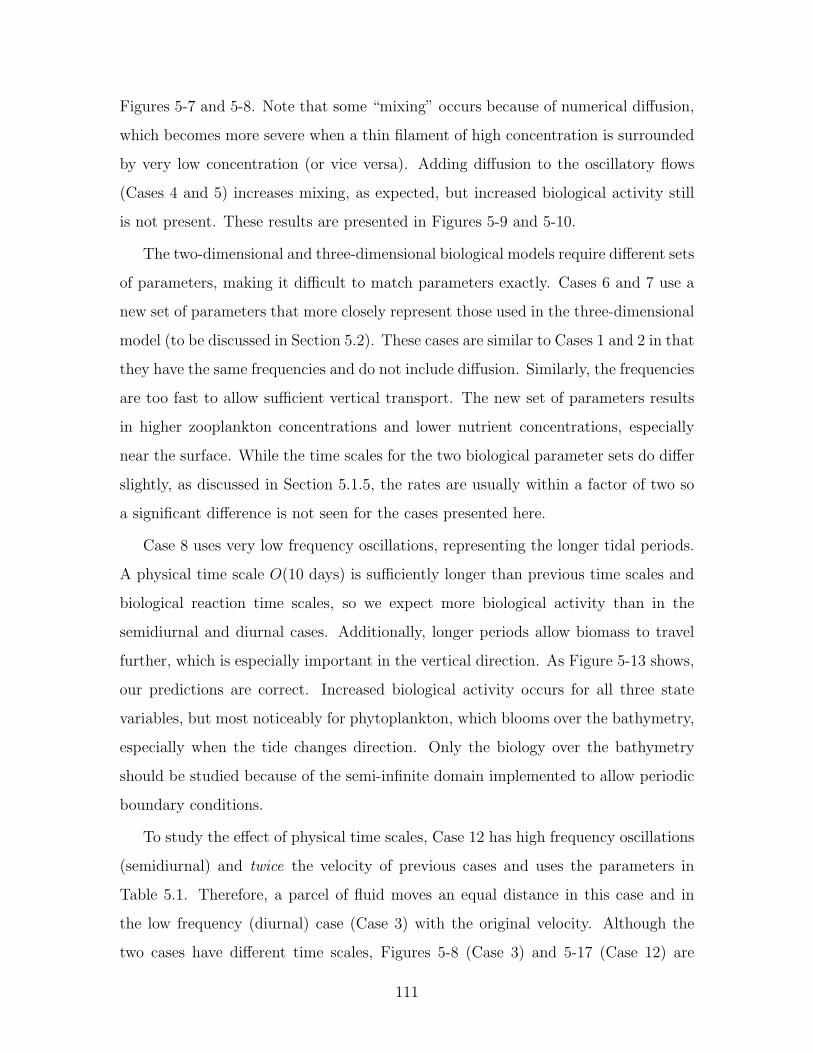
Figures 5-7 and 5-8. Note that some “mixing” occurs because of numerical diffusion,
which becomes more severe when a thin filament of high concentration is surrounded
by very low concentration (or vice versa). Adding diffusion to the oscillatory flows
(Cases 4 and 5) increases mixing, as expected, but increased biological activity still
is not present. These results are presented in Figures 5-9 and 5-10.
The two-dimensional and three-dimensional biological models require different sets
of parameters, making it difficult to match parameters exactly. Cases 6 and 7 use a
new set of parameters that more closely represent those used in the three-dimensional
model (to be discussed in Section 5.2). These cases are similar to Cases 1 and 2 in that
they have the same frequencies and do not include diffusion. Similarly, the frequencies
are too fast to allow sufficient vertical transport. The new set of parameters results
in higher zooplankton concentrations and lower nutrient concentrations, especially
near the surface. While the time scales for the two biological parameter sets do differ
slightly, as discussed in Section 5.1.5, the rates are usually within a factor of two so
a significant difference is not seen for the cases presented here.
Case 8 uses very low frequency oscillations, representing the longer tidal periods.
A physical time scale O(10 days) is sufficiently longer than previous time scales and
biological reaction time scales, so we expect more biological activity than in the
semidiurnal and diurnal cases. Additionally, longer periods allow biomass to travel
further, which is especially important in the vertical direction. As Figure 5-13 shows,
our predictions are correct. Increased biological activity occurs for all three state
variables, but most noticeably for phytoplankton, which blooms over the bathymetry,
especially when the tide changes direction. Only the biology over the bathymetry
should be studied because of the semi-infinite domain implemented to allow periodic
boundary conditions.
To study the effect of physical time scales, Case 12 has high frequency oscillations
(semidiurnal) and twice the velocity of previous cases and uses the parameters in
Table 5.1. Therefore, a parcel of fluid moves an equal distance in this case and in
the low frequency (diurnal) case (Case 3) with the original velocity. Although the
two cases have different time scales, Figures 5-8 (Case 3) and 5-17 (Case 12) are
111
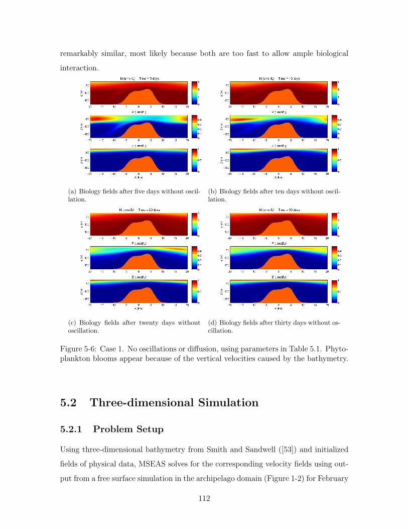
remarkably similar, most likely because both are too fast to allow ample biological
interaction.
(a) Biology fields after five days without oscil-lation.
(b) Biology fields after ten days without oscil-lation.
(c) Biology fields after twenty days withoutoscillation.
(d) Biology fields after thirty days without os-cillation.
Figure 5-6: Case 1. No oscillations or diffusion, using parameters in Table 5.1. Phyto-plankton blooms appear because of the vertical velocities caused by the bathymetry.
5.2 Three-dimensional Simulation
5.2.1 Problem Setup
Using three-dimensional bathymetry from Smith and Sandwell ([53]) and initialized
fields of physical data, MSEAS solves for the corresponding velocity fields using out-
put from a free surface simulation in the archipelago domain (Figure 1-2) for February
112
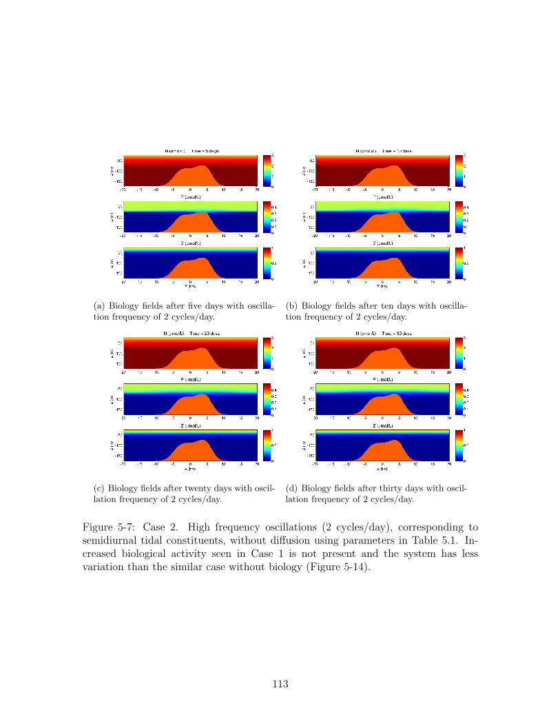
(a) Biology fields after five days with oscilla-tion frequency of 2 cycles/day.
(b) Biology fields after ten days with oscilla-tion frequency of 2 cycles/day.
(c) Biology fields after twenty days with oscil-lation frequency of 2 cycles/day.
(d) Biology fields after thirty days with oscil-lation frequency of 2 cycles/day.
Figure 5-7: Case 2. High frequency oscillations (2 cycles/day), corresponding tosemidiurnal tidal constituents, without diffusion using parameters in Table 5.1. In-creased biological activity seen in Case 1 is not present and the system has lessvariation than the similar case without biology (Figure 5-14).
113
(a) Biology fields after five days with oscilla-tion frequency of 1 cycle/day.
(b) Biology fields after ten days with oscilla-tion frequency of 1 cycle/day.
(c) Biology fields after twenty days with oscil-lation frequency of 1 cycle/day.
(d) Biology fields after thirty days with oscil-lation frequency of 1 cycle/day.
Figure 5-8: Case 3. Low frequency oscillations (1 cycle/day), corresponding to diurnaltidal constituents, without diffusion using parameters in Table 5.1. Increased biolog-ical activity similar to Case 1 is still not present and the system has less variationthan the similar case without biology (Figure 5-15).
114

(a) Biology fields after five days with oscilla-tion frequency of 2 cycles/day.
(b) Biology fields after ten days with oscilla-tion frequency of 2 cycles/day.
(c) Biology fields after twenty days with oscil-lation frequency of 2 cycles/day.
(d) Biology fields after thirty days with oscil-lation frequency of 2 cycles/day.
Figure 5-9: Case 4. High frequency oscillations (2 cycles/day), corresponding tosemidiurnal tidal constituents, with diffusion using parameters from Table 5.1 leadsto more mixing than Case 2.
115

(a) Biology fields after five days with oscilla-tion frequency of 1 cycle/day.
(b) Biology fields after ten days with oscilla-tion frequency of 1 cycle/day.
(c) Biology fields after twenty days with oscil-lation frequency of 1 cycle/day.
(d) Biology fields after thirty days with oscil-lation frequency of 1 cycle/day.
Figure 5-10: Case 5. Low frequency oscillations (1 cycle/day), corresponding todiurnal tidal constituents, with diffusion using parameters from Table 5.1 leads tomore mixing than Case 3.
116

(a) Biology fields after five days with oscilla-tion frequency of 2 cycles/day.
(b) Biology fields after ten days with oscilla-tion frequency of 2 cycles/day.
(c) Biology fields after twenty days with oscil-lation frequency of 2 cycles/day.
(d) Biology fields after thirty days with oscil-lation frequency of 2 cycles/day.
Figure 5-11: Case 6. High frequency oscillations (2 cycles/day), corresponding tosemidiurnal tidal constituents, without diffusion using parameters matching the three-dimensional case.
117
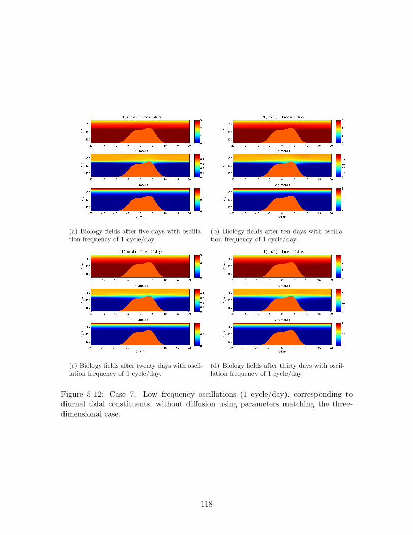
(a) Biology fields after five days with oscilla-tion frequency of 1 cycle/day.
(b) Biology fields after ten days with oscilla-tion frequency of 1 cycle/day.
(c) Biology fields after twenty days with oscil-lation frequency of 1 cycle/day.
(d) Biology fields after thirty days with oscil-lation frequency of 1 cycle/day.
Figure 5-12: Case 7. Low frequency oscillations (1 cycle/day), corresponding todiurnal tidal constituents, without diffusion using parameters matching the three-dimensional case.
118

(a) Biology fields after five days with oscilla-tion frequency of 0.1 cycles/day.
(b) Biology fields after ten days with oscilla-tion frequency of 0.1 cycles/day.
(c) Biology fields after twenty days with oscil-lation frequency of 0.1 cycles/day.
(d) Biology fields after thirty days with oscil-lation frequency of 0.1 cycles/day.
Figure 5-13: Case 8. Very low frequency oscillations (0.1 cycles/day), correspondingto the longer tidal constituents, without diffusion using parameters from Table 5.1.Increased biological activity is seen, as tidal period is similar to the biological timescale.
119
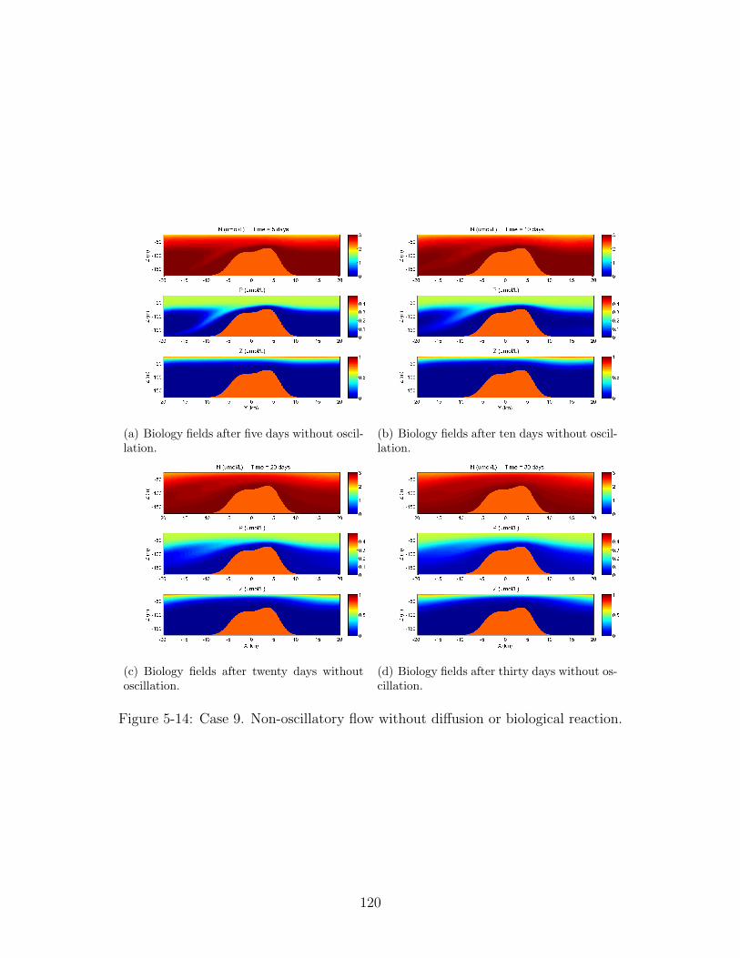
(a) Biology fields after five days without oscil-lation.
(b) Biology fields after ten days without oscil-lation.
(c) Biology fields after twenty days withoutoscillation.
(d) Biology fields after thirty days without os-cillation.
Figure 5-14: Case 9. Non-oscillatory flow without diffusion or biological reaction.
120
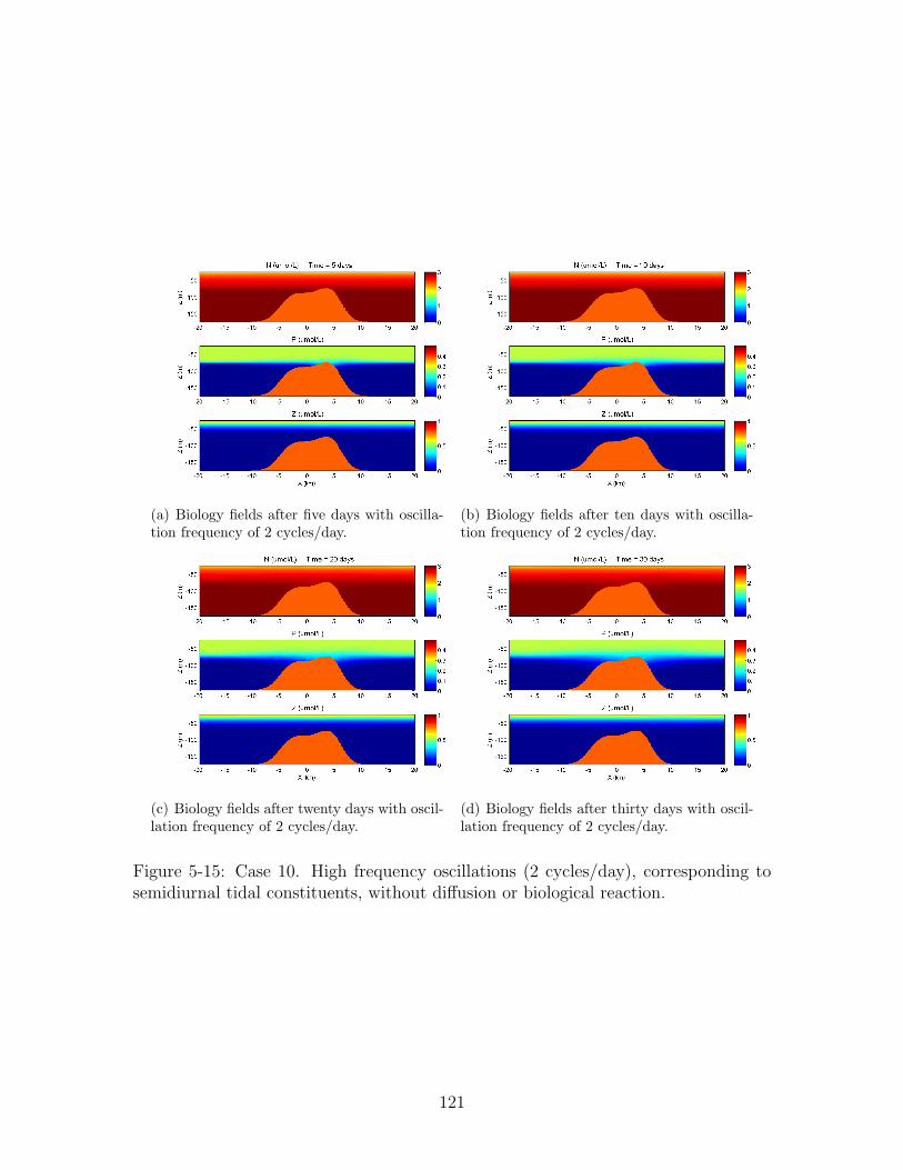
(a) Biology fields after five days with oscilla-tion frequency of 2 cycles/day.
(b) Biology fields after ten days with oscilla-tion frequency of 2 cycles/day.
(c) Biology fields after twenty days with oscil-lation frequency of 2 cycles/day.
(d) Biology fields after thirty days with oscil-lation frequency of 2 cycles/day.
Figure 5-15: Case 10. High frequency oscillations (2 cycles/day), corresponding tosemidiurnal tidal constituents, without diffusion or biological reaction.
121

(a) Biology fields after five days with oscilla-tion frequency of 1 cycle/day.
(b) Biology fields after ten days with oscilla-tion frequency of 1 cycle/day.
(c) Biology fields after twenty days with oscil-lation frequency of 1 cycle/day.
(d) Biology fields after thirty days with oscil-lation frequency of 1 cycle/day.
Figure 5-16: Case 11. Low frequency oscillations (1 cycle/day), corresponding todiurnal tidal constituents, without diffusion or biological reaction.
122
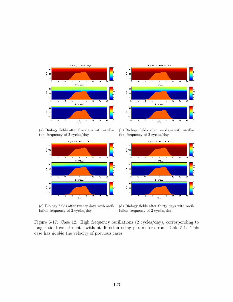
(a) Biology fields after five days with oscilla-tion frequency of 2 cycles/day.
(b) Biology fields after ten days with oscilla-tion frequency of 2 cycles/day.
(c) Biology fields after twenty days with oscil-lation frequency of 2 cycles/day.
(d) Biology fields after thirty days with oscil-lation frequency of 2 cycles/day.
Figure 5-17: Case 12. High frequency oscillations (2 cycles/day), corresponding tolonger tidal constituents, without diffusion using parameters from Table 5.1. Thiscase has double the velocity of previous cases.
123

and March 2009. The simulation is forced with combination of wind stress from the
Coupled Ocean/Atmosphere Mesoscale Prediction System (COAMPS, developed by
the Naval Research Laboratory) and heat flux and Eliassen–Palm (E–P) flux from
the U.S. Navy Operational Global Atmospheric Prediction System (NOGAPS) model.
Large-scale open boundary conditions are weakly forced by the Hybrid Coordinate
Ocean Model (HYCOM) fields. All simulations are forced with Generalized Inverse
High-Resolution Barotropic Tides [38]. Remotely-sensed sea surface height anomalies
and sea surface temperature are the only synoptic data utilized for initialization and
assimilation, as no hydrographic data are currently available. To include biology, we
initialized the biological fields in MSEAS to enable analysis of coupled physics and
biology in the Philippine Archipelago as part of the PhilEx program. The details of
this process and the resulting solutions are discussed in this section.
5.2.2 Biology Initialization
After simulations for physics in the Philippine Archipelago were sufficiently tuned,
coupled physics-biology model simulation studies and forecasts were initiated, prompt-
ing the need for initial conditions for the biological variables used in the model. The
Dusenberry-Lermusiaux biological model [6], discussed in Chapter 2, is used to model
the advection, diffusion, and reaction of six state variables: chlorophyll, nitrate, am-
monium, detritus, phytoplankton and zooplankton. Thus, we need three-dimensional
fields of each of these variables to initialize the model. Our new methodology to do
so is described next.
A combination of biogeochemical, climatological, satellite, and historical data was
used for initialization, as data is extremely limited in the Philippines. We gathered
MODIS weekly calibrated satellite images of chlorophyll-a concentration for February
and March 2009 as ASCII files from OceanWatch [44]. This satellite data was mapped
onto the modeling grid also used for physics. Cloud cover prevented complete coverage
in the region, so the first two weeks of February were combined by averaging any point
present in both the weeks and taking the value of whichever point is present otherwise.
Even when two weeks of data were merged, full coverage was still not achieved, so the
124

field was smoothly interpolated to give full coverage [24]. This completed the initial
surface field for the euphotic-zone integrated chlorophyll for February. We applied
the same techniques to the MODIS satellite data for the last week of February and
the first week of March to obtain the initialized integrated surface chlorophyll field
for March.
Figure 5-18: Regions of the Philippine Archipelago with different chlorophyll profiles.Dark blue represents the South China Sea, yellow is the Sulu Sea, cyan is the Pacific,and red represents the interior seas.
To create a three-dimensional field from the surface chlorophyll, we divided the do-
main into regions (Figure 5-18) which are distinctive biologically and created a generic
profile for each (Figure 5-19). These profiles are based on experimental data [10]. We
modeled them as a combination of two “shifted” Gaussian-like curves (Equation 5.2).
B(zu) = Bo +a
σu√
2πe− (zu−zm)2
2σ2u
B(zl) = Bo +a
σu√
2πe− (zl−zm)2
2σ2l
(5.2)
where B(zu) is the profile above the deep chlorophyll maximum, B(zl) is the profile
125

below the deep chlorophyll maximum, Bo is the background value, σu is the standard
deviation of the upper profile, σl determines the spread of the lower profile, a deter-
mines the peak value and zm is the depth of the deep chlorophyll maximum. Note
that the two profiles meet and are continuous at zm. We then fit (scaled) these ana-
lytical profiles (Equation 5.2) at each point so that the integrated chlorophyll value
(from the merged satellite data) matched the value of the integrated profile. Figure
5-19 shows three generic profiles for three different regions in the Philippines. The
deep chlorophyll maximum is highest for the Visayan Sea and other interior seas and
lowest for the Pacific Ocean.
0 0.05 0.1 0.15 0.2 0.25 0.3 0.35 0.4−200
−180
−160
−140
−120
−100
−80
−60
−40
−20
0Generic Chl Profiles for the Philippines Archipelago
Chl (mg/m3)
Dep
th (
m)
SCS/SuluInterior SeasPacific
Figure 5-19: Example of generic profiles for chlorophyll were scaled according to thesurface integrated chlorophyll value from satellite images. xs distinguish peaks fromthe background value.
We then generated initial fields of nitrate (NO−3 ) by using Objective Analysis (OA)
methods to obtain profiles from climatology data (horizontal fields in 1o resolution for
specified depth levels) from World Ocean Atlas [1] for February and March. For future
simulations, we will use a novel Objective Analysis approach [3] based on the Fast
Marching Method, which accounts for the coastline constraints by using the optimal
path length (minimum distance between two points without going across landforms),
an important consideration for a domain with several islands and complex coastlines,
126
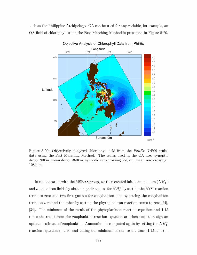
such as the Philippine Archipelago. OA can be used for any variable, for example, an
OA field of chlorophyll using the Fast Marching Method is presented in Figure 5-20.
Objective Analysis of Chlorophyll Data from PhilEx
Longitude
Latitude
Surface 0m
Figure 5-20: Objectively analyzed chlorophyll field from the PhilEx IOP09 cruisedata using the Fast Marching Method. The scales used in the OA are: synopticdecay–90km, mean decay–360km, synoptic zero crossing–270km, mean zero crossing–1080km.
In collaboration with the MSEAS group, we then created initial ammonium (NH+4 )
and zooplankton fields by obtaining a first guess forNH+4 by setting theNO−3 reaction
terms to zero and two first guesses for zooplankton, one by setting the zooplankton
terms to zero and the other by setting the phytoplankton reaction terms to zero [24],
[34]. The minimum of the result of the phytoplankton reaction equation and 1.15
times the result from the zooplankton reaction equation are then used to assign an
updated estimate of zooplankton. Ammonium is computed again by setting the NH+4
reaction equation to zero and taking the minimum of this result times 1.15 and the
127
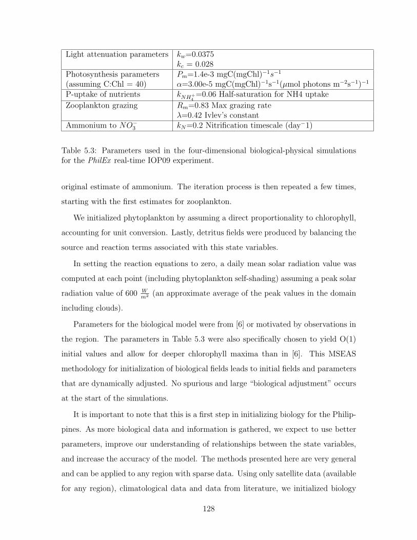
Light attenuation parameters kw=0.0375kc = 0.028
Photosynthesis parameters Pm=1.4e-3 mgC(mgChl)−1s−1
(assuming C:Chl = 40) α=3.00e-5 mgC(mgChl)−1s−1(µmol photons m−2s−1)−1
P-uptake of nutrients kNH+4
=0.06 Half-saturation for NH4 uptake
Zooplankton grazing Rm=0.83 Max grazing rateλ=0.42 Ivlev’s constant
Ammonium to NO−3 kN=0.2 Nitrification timescale (day−1)
Table 5.3: Parameters used in the four-dimensional biological-physical simulationsfor the PhilEx real-time IOP09 experiment.
original estimate of ammonium. The iteration process is then repeated a few times,
starting with the first estimates for zooplankton.
We initialized phytoplankton by assuming a direct proportionality to chlorophyll,
accounting for unit conversion. Lastly, detritus fields were produced by balancing the
source and reaction terms associated with this state variables.
In setting the reaction equations to zero, a daily mean solar radiation value was
computed at each point (including phytoplankton self-shading) assuming a peak solar
radiation value of 600 Wm2 (an approximate average of the peak values in the domain
including clouds).
Parameters for the biological model were from [6] or motivated by observations in
the region. The parameters in Table 5.3 were also specifically chosen to yield O(1)
initial values and allow for deeper chlorophyll maxima than in [6]. This MSEAS
methodology for initialization of biological fields leads to initial fields and parameters
that are dynamically adjusted. No spurious and large “biological adjustment” occurs
at the start of the simulations.
It is important to note that this is a first step in initializing biology for the Philip-
pines. As more biological data and information is gathered, we expect to use better
parameters, improve our understanding of relationships between the state variables,
and increase the accuracy of the model. The methods presented here are very general
and can be applied to any region with sparse data. Using only satellite data (available
for any region), climatological data and data from literature, we initialized biology
128

fields for six state variables.
5.2.3 Results
The ocean field estimates from MSEAS show increased activity above bathymetric
features. For our purposes, we will focus on the San Bernardino Strait. Plots of
nitrate, phytoplankton, and zooplankton estimates along a cross-section of the San
Bernardino Strait (along 12.13oN, 123.98oE to 13.33oN, 124.66oE) are presented in
Figure 5-21. From February 2, 2009 to March 5, 2009, plots were analyzed for noon
and midnight of each day. From these, we see that nitrate consistently has higher
values across and above the strait under 50m (Figure 5-21(a)), with higher concentra-
tion tongues sometimes appearing over the sloped bathymetry, as in Figure 5-21(b).
Phytoplankton always had maximum values above the bathymetry (Figure 5-21(c)),
which sometimes extended toward the Pacific Ocean (Figure 5-21(d)). Zooplankton
had similar behavior, with consistent maximum values above the bathymetry (Fig-
ure 5-21(e)) that sometimes extended further northeast (Figure 5-21(f)). Other state
variables were similar qualitatively to those presented here.
5.3 Discussion and Future Work
The results from the two-dimensional and three-dimensional cases are very difficult
to compare, even qualitatively, because of the varying levels of complexity between
the two. Case 8, which has a much longer tidal period than other cases, is the
most similar to the three-dimensional results, with increased biological activity fo-
cused over the bathymetry sometimes extending towards the Pacific Ocean. Cases 2
through 7 of the two-dimensional model are not very similar to the three-dimensional
results, which may indicate that the lower frequencies dominate the biological activ-
ity. However, these differences could also be attributed to having different flow fields
(two-dimensional versus three-dimensional), bathymetries, and initial conditions. The
two-dimensional results did clearly show that long physical time scales, compared to
129
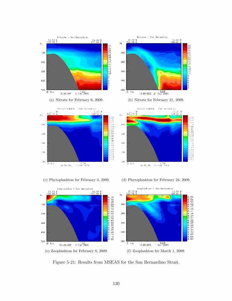
(a) Nitrate for February 6, 2009. (b) Nitrate for February 21, 2009.
(c) Phytoplankton for February 4, 2009. (d) Phytoplankton for February 24, 2009.
(e) Zooplankton for February 8, 2009. (f) Zooplankton for March 1, 2009.
Figure 5-21: Results from MSEAS for the San Bernardino Strait.
130
the biological reaction time scales, allowed more biological activity throughout the
water column.
Additionally, a new method for initializing the biological fields was developed and
utilized. With region-specific chlorophyll profiles, the three-dimensional chlorophyll
field developed from satellite data accounted for regional differences, which can be
vast for a domain like the Philippine Archipelago.
For future work, an averaged velocity field from MSEAS could be used in the
two-dimensional simulation for better comparison. Additionally, the initialized fields
could be matched more closely. A noticeable difference seems to be the critical depth
(where phytoplankton receives enough light to grow); it is much lower in the three-
dimensional model. For the two-dimensional case, it would be interesting to investi-
gate cases which combine several different tidal frequencies. These results would likely
be dominated by the lowest frequency, which allow the furthest vertical transport.
When nutrient-rich water is able to reach shallow depths where nutrients have been
depleted, increased biological activity and blooms are likely because of the increase
in food sources.
131

132

Chapter 6
Conclusion
In this thesis, we presented research toward understanding coupled physics-biology
processes in ocean straits. We performed new analytical studies and higher-order
simulations of idealized dynamics that are relevant to generic biology in straits and
applied them to the San Bernardino Strait in the Philippine Archipelago with tidal
forcing.
In Chapter 2, we motivated our research, discussing the importance of under-
standing coupled physics and biology interactions and the sparsity of data, especially
in the Philippine domain. Further, we completed an overview of lower trophic level
biological models in the ocean, including the Nutrient-Phytoplankton-Zooplankton
(NPZ) model and a more complicated six state variable model. We also discussed the
validity of NPZ models, explained the reaction terms, and compared different ways
of modeling biological reactions.
In Chapter 3, we performed novel global equilibrium and local stability analyses
for the NPZ model in terms of system parameters with and without physics. This in-
cluded finding and classifying equilibria states as stable or unstable, developing a new
method of determining appropriate parameter values given some known parameter
values, and specifying critical stability depths and regions where stability proper-
ties change. Phase portraits verified our predictions and simulations in the domain
(including flow). They indicated that the stability analysis for the regime without
physics gives a conservative range of appropriate parameter values, as advection, and
133
especially diffusion, act to stabilize the biological dynamics.
In Chapter 4, we developed, verified, and analyzed a two-dimensional physical-
biological model. We presented and studied a novel numerical scheme to solve the
NPZ equations for physical-biological modeling. The new scheme combines Arakawa
C-grid with masking for easy implementation of boundary conditions, the operator
splitting method for computational efficiency and the WENO scheme to avoid oscil-
lations in advection-dominated flows. We showed that the WENO scheme was also
less numerically diffusive and more computationally efficient than the donor-cell, hy-
brid, and classic central difference schemes. The central difference scheme produced
oscillatory results when tracers accumulated at the boundary and was shown to be ap-
propriate only for smooth problems. The results from the donor cell scheme were not
oscillatory because enough numerical diffusion in the system smoothed the discontinu-
ities. A hybrid scheme, which combines the donor-cell and central difference scheme,
depended on a critical value to avoid oscillations, making it still more diffusive than
WENO scheme and requiring tuning of a case-specific parameter. Additionally, the
WENO scheme was more computationally efficient for comparable resolution, which
is important when resolving biological features. A comparison to an independent
simulation using Discontinuous Galerkin on an unstructured grid showed excellent
agreement, suggesting that both schemes are accurate.
In Chapter 5, we applied the physics-biology model to a realistic representation
of the San Bernardino Strait in the Philippine Archipelago under the influence of
tidal forces and compared the results to a high fidelity three-dimensional model from
MSEAS. First, we conducted new studies of the effect of tides on biology in a test case
motivated by the San Bernardino Strait in both two and three dimensions. Different
frequencies, parameters, and levels of diffusion were examined for the two-dimensional
case. For the three-dimensional case, we proposed a new method of initializing bio-
logical variables for regions with sparse data, which includes objective analysis and
region-specific profiles. Examining different frequencies of physical forcing (e.g. tides)
in the two-dimensional case revealed that faster oscillations had less effect than slower
oscillations. The time scale of this motion was too short (compared to the biological
134
time scales) to allow phytoplankton to bloom.
The results presented serve as preparation for future work. The two-dimensional
idealized numerical simulation can be used to analyze interaction between physics
and biology for many different straits and physical features, simply by implementing
the appropriate parameters and flow field. The method to analyze the stability of
the NPZ model should be performed to ensure effects seen are realistic results of
the interactions between physics and biology. Additionally, the initialization of the
biological fields for the three-dimensional model is very general and is useful for many
regions and many different models.
More specifically, additional physical features in the San Bernardino Strait should
be isolated and examined in both the two-dimensional and three-dimensional models
to identify their effect on biology. As PhilEx continues, more biological data will be
available and those results should be compared to the results from the computational
models and used to improve future modeling of physical-biological interactions in the
San Bernardino Strait.
135

136
Appendix A
Number of valid Z equilibrium
based on ρ and s
The following figures hold NT constant for NT = 2, 2.2, and 3 µmol/L (values in each
of the different stability regions). For each NT value, there is a figure showing s, ρ,
and ρ2 with β versus zooplankton concentration Z (these expressions are defined in
Equation 3.4). Figures are shown for the entire depth range (in terms of β) and also
focused on the depth region where the stability transitions occur.
137

Region 1 Region 2 Region 3Z 0 ≤ β < βc1 βc1 < β < βc2 βc2 < β ≤ u
−∞ < z < zc1 zc1 < z < zc2 zc2 < z ≤ 0
s > 0 s < 0 s < 00 < NT < NTcρ ρ < 0 ρ < 0 ρ > 0
No solutions One solution One solutions < 0 s < 0 s < 0
NTcρ < NT < NTcs ρ < 0 ρ > 0 ρ > 0One solution One solution One solution
s < 0 s > 0 s > 0NT > NTcs ρ > 0 ρ > 0 ρ > 0
One solution Two solutions Two solutions
Table A.1: Number of zooplankton equilibrium based on total biomass (NT ), depth,and the sign of ρ and s. Figures included in this Appendix show that ρ and s can beplotted easily to determine the number of solutions for a given depth.
0.1 0.2 0.3 0.4 0.5 0.6b
2
4
6
8
10
Z
NT=2
r2
s
r
β
ρ
ρ2
Figure A-1: ρ, s, and ρ2 for NT = 2 µmol/L over entire depth range β. Transitionsonly occur for very small β (deep water), shown in Figure A-2.
138

0.01 0.02 0.03 0.04 0.05b
- 0.15
- 0.10
- 0.05
0.05
0.10
Z
NT=2
r2
s
r
β
ρ
ρ2
Figure A-2: At β = 0, ρ < 0 and s > 0, so no solutions are present. After approx-imately β = 0.01, s < 0 and one solution appears. At about β = 0.0275, ρ > 0 andonly one solution is still present. This corresponds to NT = 2 µmol/L, which is thesecond row of Table A.1.
0.1 0.2 0.3 0.4 0.5 0.6b
2
4
6
8
10
Z
NT=2.2
r2
s
r
β
ρ
ρ2
Figure A-3: ρ, s, and ρ2 for NT = 2.2 µmol/L over entire depth range β. Transitionsonly occur for very small β (deep water), shown in Figure A-4.
139
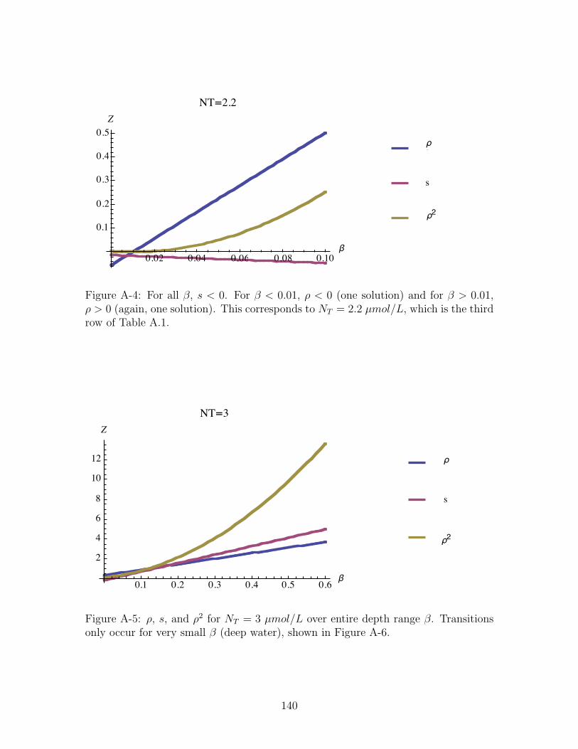
0.02 0.04 0.06 0.08 0.10b
0.1
0.2
0.3
0.4
0.5
Z
NT=2.2
r2
s
r
β
ρ
ρ2
Figure A-4: For all β, s < 0. For β < 0.01, ρ < 0 (one solution) and for β > 0.01,ρ > 0 (again, one solution). This corresponds to NT = 2.2 µmol/L, which is the thirdrow of Table A.1.
0.1 0.2 0.3 0.4 0.5 0.6b
2
4
6
8
10
12
Z
NT=3
r 2
s
r
β
ρ
ρ2
Figure A-5: ρ, s, and ρ2 for NT = 3 µmol/L over entire depth range β. Transitionsonly occur for very small β (deep water), shown in Figure A-6.
140
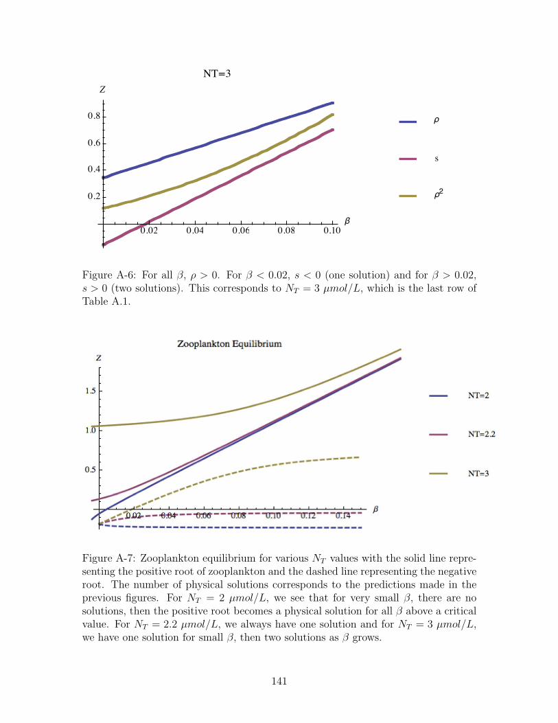
0.02 0.04 0.06 0.08 0.10b
0.2
0.4
0.6
0.8
Z
NT=3
r2
s
r
β
ρ
ρ2
Figure A-6: For all β, ρ > 0. For β < 0.02, s < 0 (one solution) and for β > 0.02,s > 0 (two solutions). This corresponds to NT = 3 µmol/L, which is the last row ofTable A.1.
β
Figure A-7: Zooplankton equilibrium for various NT values with the solid line repre-senting the positive root of zooplankton and the dashed line representing the negativeroot. The number of physical solutions corresponds to the predictions made in theprevious figures. For NT = 2 µmol/L, we see that for very small β, there are nosolutions, then the positive root becomes a physical solution for all β above a criticalvalue. For NT = 2.2 µmol/L, we always have one solution and for NT = 3 µmol/L,we have one solution for small β, then two solutions as β grows.
141
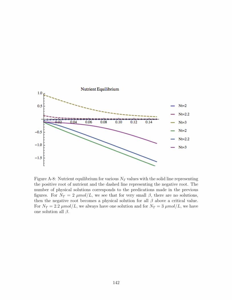
β
Figure A-8: Nutrient equilibrium for various NT values with the solid line representingthe positive root of nutrient and the dashed line representing the negative root. Thenumber of physical solutions corresponds to the predications made in the previousfigures. For NT = 2 µmol/L, we see that for very small β, there are no solutions,then the negative root becomes a physical solution for all β above a critical value.For NT = 2.2 µmol/L, we always have one solution and for NT = 3 µmol/L, we haveone solution all β.
142

Appendix B
Phase Portraits
We created phase portraits of P versus Z using the nonlinear coupled NPZ equations
without advection or diffusion (Equations 3.1). This appendix shows these phase
portraits for NT = 2, 3, 5, and 8 µmol/L. For the last three values, phase portraits
are shown both for the full range of values as well as for a smaller range surrounding
the analytical equilibrium point (NT = 2 µmol/L has an equilibrium point outside
of the physical region and therefore is not shown). The x-axis is concentration of
zooplankton Z while the y-axis is phytoplankton concentration P . The equilibrium
points are listed for each depth level and NT value. Only values under the line
P = NT −Z are considered, as this defines the region where the solutions are physical
(from the restriction NT = N + P + Z).
Stability z = 0m z = −25m z = −50m
NT = 2 µmol/L U U UNT = 3 µmol/L S S SNT = 5 µmol/L S U UNT = 8 µmol/L S U U
Table B.1: Predicted stability of the phase portraits for P versus Z.
143

NT = 2EquilibriumPoint
Whole Range Around Equilibrium Point
x−axis is Z, y−axis is P x−axis is Z, y−axis is P
z=0P=2.2314,Z=-0.2306Unstable
N/A
z=-25P=2.2314,Z=-0.2283Unstable
N/A
z=-50P=2.2314,Z=-0.2208Unstable
N/A
144
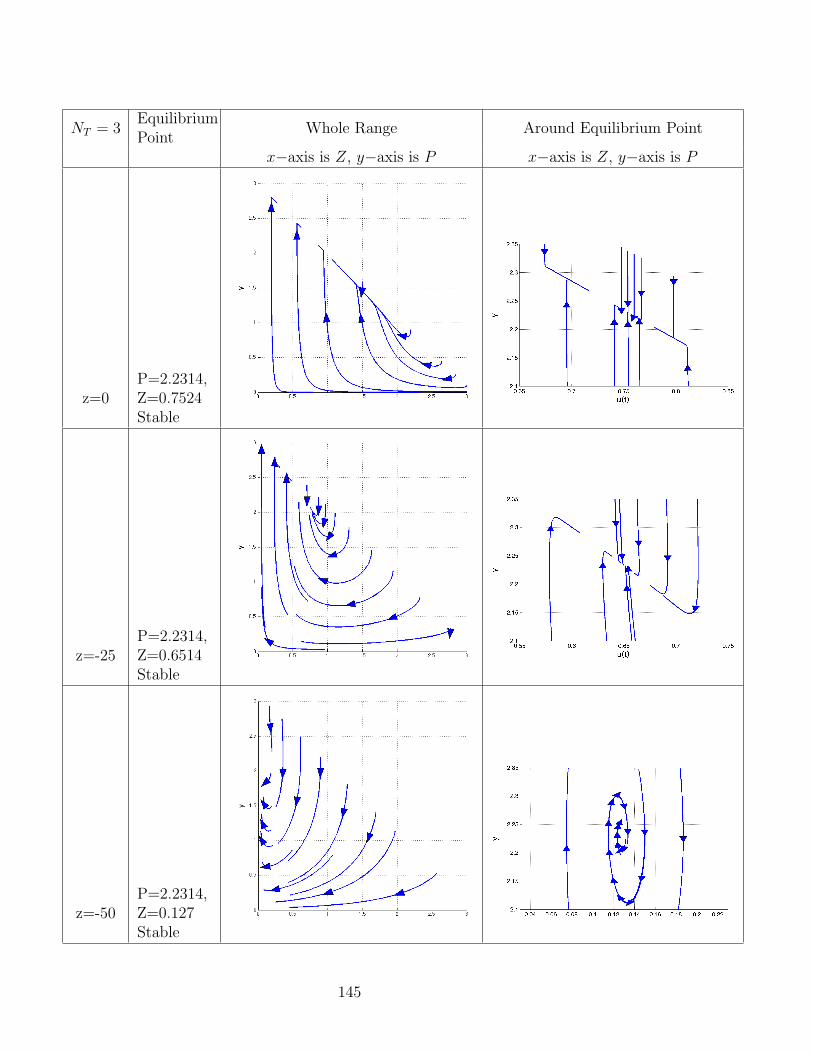
NT = 3EquilibriumPoint
Whole Range Around Equilibrium Point
x−axis is Z, y−axis is P x−axis is Z, y−axis is P
z=0P=2.2314,Z=0.7524Stable
z=-25P=2.2314,Z=0.6514Stable
z=-50P=2.2314,Z=0.127Stable
145

NT = 5EquilibriumPoint
Whole Range Around Equilibrium Point
x−axis is Z, y−axis is P x−axis is Z, y−axis is P
z=0P=2.2314,Z=2.6934Stable
z=-25
P=2.2314,Z=1.2639Unstable(AlmostNeutral)
z=-50P=2.2314,Z=0.1619Unstable
146
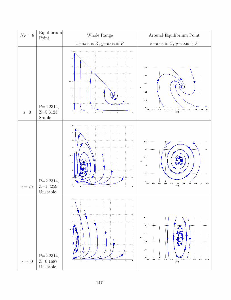
NT = 8EquilibriumPoint
Whole Range Around Equilibrium Point
x−axis is Z, y−axis is P x−axis is Z, y−axis is P
z=0P=2.2314,Z=5.3123Stable
z=-25P=2.2314,Z=1.3259Unstable
z=-50P=2.2314,Z=0.1687Unstable
147

148
Bibliography
[1] World ocean atlas 2005, data sets and products.http://www.nodc.noaa.gov/OC5/WOA05/, 2005.
[2] Multidisciplinary simulation, estimation, and assimilation systems.http://modelseas.mit.edu/, 2009.
[3] A Agarwal. Statistical field estimation and scale estimation for complex coastalregions and archipelagos. SM thesis, MIT, 2009.
[4] A Arakawa and V Lamb. Computational design of the basic dynamical pro-cesses of the ucla general circulation model. General circulation models of theatmosphere, Jan 1977.
[5] R Barber and M Hiscock. A rising tide lifts all phytoplankton: Growth responseof other phytoplankton taxa in diatom-dominated blooms. Global Biogeochem.Cycles, 20, Jan 2006.
[6] ST Besiktepe, PFJ Lermusiaux, and A Robinson. Coupled physical and biogeo-chemical data-driven simulations of massachusetts bay in late summer: real-timeand postcruise data assimilation. Journal of Marine Systems, 40:171–212, 2003.
[7] CC Chen, FK Shiah, S Chung, and K Liu. Winter phytoplankton blooms in theshallow mixed layer of the south china sea enhanced by upwelling. Journal ofMarine Systems, Jan 2006.
[8] YLL Chen, HY Chen, and CW Chung. Seasonal variability of coccolithophoreabundance and assemblage in the northern south china sea. Deep-Sea ResearchPart II, 54(14-15):1617–1633, 2007.
[9] SD Conte and C deBoor. Elementary Numerical Analysis. Apr 1972.
[10] K Cordero. Estimating integrated phytoplankton biomass in the seas around thephilippines. Unpublished Report, 2007.
[11] G Cossarini, PFJ Lermusiaux, and C Solidoro. The lagoon of venice ecosystem:Seasonal dynamics and environmental guidance with uncertainty analyses anderror subspace data assimilation. J. Geophys. Res., pages 1–79, Apr 2009.
[12] D Cushing. Upwelling and fish production. Jan 1969.
149
[13] Benoit Cushman-Roisin. Introduction to geophysical fluid dynamics. Jan 1994.
[14] EW Dijkstra. A note on two problems in connexion with graphs. NumerischeMathematik, Jan 1959.
[15] MJR Fasham, HW Ducklow, and SM McKelvie. A nitrogen-based model ofplankton dynamics in the oceanic mixed layer. Journal of Marine Research,48:591–639, Dec 1990.
[16] W Fennel and T Neumann. Introduction to the modelling of marine ecosystems.Jan 2004.
[17] G Flierl. Mit course notes for 12.823: Modeling coupled physics and biology inthe ocean. 2009.
[18] G Flierl and DJ McGillicuddy Jr. Chapter 4. mesoscale and submesoscalephysical–biological interactions. The Sea, 12:1–74, Nov 2002.
[19] PJS Franks. Sink or swim: Accumulation of biomass at fronts. Marine ecologyprogress series. Oldendorf, Jan 1992.
[20] PJS Franks. Npz models of plankton dynamics: their construction, coupling tophysics, and application. Journal of Oceanography, Jan 2002.
[21] PJS Franks and CC Chen. Plankton production in tidal fronts: a model ofgeorges bank in summer. Journal of Marine Research, Jan 1996.
[22] H Gao, S Feng, and Y Guan. Modelling annual cycles of primary production indifferent regions of the bohai sea. Fisheries Oceanography, 7(3-4):258–264, 1998.
[23] M Griebel, T Dornseifer, and T Neunhoeffer. Numerical simulation in fluiddynamics: a practical introduction. Jan 1997.
[24] P Haley. Personal communication. 2009.
[25] P Haley, A Robinson, and WG Leslie. Real-time forecasting in the new englandshelfbreak front: Primer97. Ocean Sciences Meeting 1998, Jan 1998.
[26] PJ Haley, PFJ Lermusiaux, A Robinson, WG Leslie, OG Logoutov, G Cossarini,XS Liang, P Moreno, SR Ramp, JD Doyle, J Bellingham, F Chavez, and S John-ston. Forecasting and reanalysis in the monterey bay/california current regionfor the autonomous ocean sampling network-ii experiment. Deep-Sea ResearchPart II, 2008.
[27] W Han, AM Moore, J Levin, B Zhang, and HG Arango. Seasonal surface oceancirculation and dynamics in the philippine archipelago region. Dynamics of At-mospheres and Oceans, Jan 2008.
150
[28] A Harten, B Engquist, S Osher, and SR Chakravarthy. Uniformly high orderaccurate essentially non-oscillatory schemes. Journal of Computational Physics,71(2):231–303, 1987.
[29] M Hayashi, T Yanagi, and ML Diego-Mcglone. Nitrogen cycling in manila bayduring dry and rainy seasons. Coastal Marine Science, 2006.
[30] E Hofmann and M Friedrichs. Predictive modeling for marine ecosystems. TheSea, 2002.
[31] LE Holmedal and T Utnes. Physical-biological interactions and their effect onphytoplankton blooms in fjords and near-coastal waters. Journal of MarineResearch, 64(1):97–122, Jan 2006.
[32] S Kimura, A Kasai, H Nakata, T Sugimoto, JH Simpson, and JVS Cheok. Bi-ological productivity of meso-scale eddies caused by frontal disturbances in thekuroshio. ICES Journal of Marine Science, 54(2):179, 1997.
[33] CM Lalli and TR Parsons. Biological Oceanography: An Introduction. Jan 1997.
[34] PFJ Lermusiaux. Personal communication. 2009.
[35] PFJ Lermusiaux. Adaptive modeling, adaptive data assimilation and adaptivesampling. Physica D: Nonlinear Phenomena, Jan 2007.
[36] PFJ Lermusiaux and A Robinson. Data assimilation via error subspace statisticalestimation. Monthly Weather Review, Jan 1999.
[37] OG Logoutov. A multigrid methodology for assimilation of measurements intoregional tidal models. Ocean Dynamics, 58(5-6):441–460, Jan 2008.
[38] OG Logoutov and PFJ Lermusiaux. Inverse barotropic tidal estimation for re-gional ocean applications. Ocean Modelling, Jan 2008.
[39] D Macıas, AP Martin, J Garca Lafuente, CM Garca, A Yool, M Bruno,A Vazquez-Escobar, A Izquierdo, DV Sein, and F Echevarra. Analysis of mixingand biogeochemical effects induced by tides on the atlantic–mediterranean flowin the strait of gibraltar through a physical–biological coupled model. Progressin Oceanography, 74(2-3):252–272, 2007.
[40] DJ Mackey, J Parslow, HW Higgins, FB Griffiths, and JE O’Sullivan. Plank-ton productivity and biomass in the western equatorial pacific: biological andphysical controls. Deep-Sea Research Part II, 42(2-3):499–533, 1995.
[41] L Menez, CL Villanoy, and LT David. Movement of water across passages con-necting philippine inland sea basins. Science Diliman, 2006.
[42] MSEAS. Mseas philex website. http://modelseas.mit.edu/Research/Straits/,2009.
151
[43] MSEAS. Mseas real time results from philex iop09. http ://mseas.mit.edu/Sea exercises/Philex IOP09/, 2009.
[44] NOAA. Oceanwatch las. http://oceanwatch.pifsc.noaa.gov/las/servlets/dataset,2009.
[45] Joseph Pedlosky. Geophysical fluid dynamics. Jan 1998.
[46] WH Press. Numerical recipes in C/C++: The Art of Scientific Computing. Jan2002.
[47] W Reed and T Hill. Triangular mesh methods for the neutron transport equation.Los Alamos Report LA-UR-73-479, Jan 1973.
[48] A Robinson, P Haley Jr, and PFJ Lermusiaux. Application of the generic harvardocean prediction system (hops) to real-time forecasting with adapative samplingoff the central california coast during aosn-ii. people.seas.harvard.edu, Jan 2004.
[49] A Robinson and PFJ Lermusiaux. Data assimilation for modeling and predictingcoupled physical-biological interactions in the sea. The Sea, 2002.
[50] IR Santos, WC Burnett, T Dittmar, IGNA Suryaputra, and J Chanton. Tidalpumping drives nutrient and dissolved organic matter dynamics in a gulf ofmexico subterranean estuary. Geochim Cosmochim Ac, 73(5):1325–1339, Jan2009.
[51] CW Shu. Essentially non-oscillatory and weighted essentially non-oscillatoryschemes for hyperbolic conservation laws. Advanced Numerical Approximationof Nonlinear Hyperbolic Equations, 1697:325–432, 1997.
[52] R Signell. Tidal dynamics and dispersion around coastal headlands. WHOI/MITJoint Program PhD Thesis, Jan 1989.
[53] WHF Smith and DT Sandwell. Global seafloor topography from satellite altime-try and ship depth soundings. Science, 277:1957–1962, 1997.
[54] R Stewart. Introduction to Physical Oceanography. Jan 2003.
[55] S Takeda, N Ramaiah, M Miki, Y Kondo, Y Yamaguchi, Y Arii, F Gomez,K Furuya, and W Takahashi. Biological and chemical characteristics of high-chlorophyll, low-temperature water observed near the sulu archipelago. Deep-SeaResearch Part II, 54(1-2):81–102, 2007.
[56] R Tian, PFJ Lermusiaux, James McCarthy, and A Robinson. A generalized prog-nostic model of marine biogeochemical-ecosystem dynamics: Structure, parame-terization, and adaptive modeling. Harvard Reports in Physical/InterdisciplinaryOcean Science #67, May 2004.
[57] M Ueckermann. Personal communication. 2009.
152

[58] M Ueckermann, PJ Haley, and PFJ Lermusiaux. Towards structured and un-structured data assimilative modeling systems for regional physical biogeochem-ical dynamics. Seventh International Workshop on Unstructured Grid NumericalModelling of Coastal, Shelf and Ocean Flows. Dartmouth, Nova Scotia, 2008.
[59] J Xu, PFJ Lermusiaux, P Haley, and W Leslie. Spatial and temporal variationsin acoustic propagation during plusnet-07 exercise in dabob bay. Proceedings ofmeetings on acoustics (POMA), Jan 2008.
[60] J Xu, K Yin, L He, X Yuan, A Ho, and P Harrison. Phosphorus limitation inthe northern south china sea during late summer: Influence of the pearl river.Deep-Sea Research Part I, Jan 2008.
[61] M Zorzano, H Mais, and L Vazquez. Numerical solution of two dimensionalfokker—planck equations. Applied Mathematics and Computation, Jan 1999.
153