Embed Size (px)
Citation preview

REPORT No.
13-04
OCEAN ENGINEERING GROUP
Application of Boundary Element Methods (BEM) to Internal
Propulsion Systems; Application to Water-jets and Inducers
Alokraj Valsaraj
August 2013
ENVIRONMENTAL AND WATER RESOURCES ENGINEERING
DEPARTMENT OF CIVIL, ARCHITECTURAL AND ENVIRONMENTAL ENG.
THE UNIVERSITY OF TEXAS AT AUSTIN
AUSTIN, TX 78712

Copyright
by
Alokraj Valsaraj
2013

The Thesis committee for Alokraj ValsarajCertifies that this is the approved version of the following thesis:
Application of Boundary Element Methods (BEM) to
Internal Propulsion Systems; Application to Water-jets
and Inducers
APPROVED BY
SUPERVISING COMMITTEE:
Spyridon A. Kinnas, Supervisor
Venkat Raman

Application of Boundary Element Methods (BEM) to
Internal Propulsion Systems; Application to Water-jets
and Inducers
by
Alokraj Valsaraj, B.E.
THESIS
Presented to the Faculty of the Graduate School of
The University of Texas at Austin
in Partial Fulfillment
of the Requirements
for the Degree of
MASTER OF SCIENCE IN ENGINEERING
THE UNIVERSITY OF TEXAS AT AUSTIN
August 2013

Dedicated to my loving parents P.Lathika and R.Valsaraj and my two
brothers Amith and Varun.

Acknowledgments
I wish to thank my advisor Prof. Spyridon A. Kinnas for his continued
guidance and support throughout my two years at UT Austin. I would also
like to thank my reader Prof. Venkat Raman for taking the time to go through
my thesis.
I also wish to thank my friends in the Ocean Engineering Group es-
pecially Ye Tian, Jay Purohit, David Menendez Aran, Chan-Hoo Jeon and
Shu-Hao Chang who made my research fun and interesting.
Finally I would like to express my gratitude to my parents P.Lathika
and R.Valsaraj and my two brothers Varun and Amith for their constant
encouragement and support in all aspects of my life.
This work was supported by the U.S. Office of Naval Research (Contract
N00014-10-1-0931) and members of the Phase VI of the Consortium on Cavi-
tation Performance of High Speed Propulsors: American Bureau of Shipping,
Kawasaki Heavy Industry Ltd., Rolls-Royce Marine AB, Rolls-Royce Marine
AS, SSPA AB, Andritz Hydro GmbH, Wartsila Netherlands B.V., Wartsila
Norway AS, Wartsila Lips Defense S.A.S. and Wartsila CME Zhenjiang Pro-
peller Co. Ltd.
v

Application of Boundary Element Methods (BEM) to
Internal Propulsion Systems; Application to Water-jets
and Inducers
Alokraj Valsaraj, M.S.E.
The University of Texas at Austin, 2013
Supervisor: Spyridon A. Kinnas
A panel method derived from inviscid irrotational flow theory and uti-
lizing hyperboloid panels is developed and applied to the simulation of steady
fully wetted flows inside water-jet pumps and rocket engine inducers. The
source and dipole influence coefficients of the hyperboloid panels are computed
using Gauss quadrature.
The present method solves the boundary value problem subject to a
uniform inflow directly by discretizing the blade, casing/shroud and hub ge-
ometries with panels. The Green’s integral equation and the influence coeffi-
cients for the water-jet/inducer problem are defined and solved by allocating
constant strength sources and dipoles on the blade, hub and casing surfaces
and constant strength dipoles on the shed wake sheets from the rotor/ sta-
tor blades. The rotor- stator interaction is accomplished using an iterative
procedure which considers the effect between the rotor and the stator, via
circumferentially averaged induced velocities.
vi

Finally, the hydrodynamic performance predictions for the water-jet
pump and the inducer from the present method are validated against exist-
ing experimental data and numerical results from Reynolds Averaged Navier-
Stokes (RANS) solvers .
vii
Table of Contents
Acknowledgments v
Abstract vi
List of Figures x
Nomenclature xviii
Chapter 1. Introduction 1
1.1 Introduction . . . . . . . . . . . . . . . . . . . . . . . . . . . . 1
1.2 Literature Review . . . . . . . . . . . . . . . . . . . . . . . . . 2
1.3 Objectives . . . . . . . . . . . . . . . . . . . . . . . . . . . . . 5
1.4 Organization . . . . . . . . . . . . . . . . . . . . . . . . . . . . 6
Chapter 2. Methodology 7
2.1 Governing Equations . . . . . . . . . . . . . . . . . . . . . . . 7
2.2 Numerical Method . . . . . . . . . . . . . . . . . . . . . . . . 10
2.2.1 Rotor only problem . . . . . . . . . . . . . . . . . . . . 10
2.2.2 Stator only problem . . . . . . . . . . . . . . . . . . . . 12
2.3 Boundary conditions . . . . . . . . . . . . . . . . . . . . . . . 12
2.4 Numerical evaluation of influence coefficients . . . . . . . . . . 13
2.4.1 Gauss quadrature . . . . . . . . . . . . . . . . . . . . . 14
2.4.2 Non-planar quadrilateral . . . . . . . . . . . . . . . . . 15
2.4.3 Casing only problem . . . . . . . . . . . . . . . . . . . . 18
Chapter 3. Numerical Analysis of Water-jets 23
3.1 Nondimensional Coefficients . . . . . . . . . . . . . . . . . . . 23
3.2 Rotor only Case . . . . . . . . . . . . . . . . . . . . . . . . . . 24
3.2.1 Rotor with cylindrical casing . . . . . . . . . . . . . . . 24
viii

3.2.2 ONR-AXWJ2 Rotor Case . . . . . . . . . . . . . . . . 33
3.3 Stator only Case . . . . . . . . . . . . . . . . . . . . . . . . . . 41
3.4 Rotor-stator interaction . . . . . . . . . . . . . . . . . . . . . . 47
Chapter 4. Numerical Analysis of Inducers 57
4.1 Introduction . . . . . . . . . . . . . . . . . . . . . . . . . . . . 57
4.2 Designed Inducer . . . . . . . . . . . . . . . . . . . . . . . . . 58
4.3 Industry Inducer . . . . . . . . . . . . . . . . . . . . . . . . . . 66
4.4 Cavitating runs . . . . . . . . . . . . . . . . . . . . . . . . . . 73
Chapter 5. Conclusions and future work 78
5.1 Conclusions . . . . . . . . . . . . . . . . . . . . . . . . . . . . 78
5.2 Future work . . . . . . . . . . . . . . . . . . . . . . . . . . . . 80
Appendix 81
Appendix 1. Formulation of 2D and 3D Influence Coefficients 82
1.1 2D Influence Coefficients . . . . . . . . . . . . . . . . . . . . . 82
1.2 3D Influence Coefficients . . . . . . . . . . . . . . . . . . . . . 82
Bibliography 84
Vita 88
ix

List of Figures
1.1 A high-speed police vessel utilizing water-jet propulsion. . . . 2
1.2 A water-jet propulsion system utilized for high-speed vessels. . 3
1.3 Schematic sketch of a water-jet propulsion system (from Chang,2012). . . . . . . . . . . . . . . . . . . . . . . . . . . . . . . . 3
2.1 Coordinate systems utilized for the analysis of a water-jet propul-sion system (Kinnas et al. 2012) . . . . . . . . . . . . . . . . . 9
2.2 Diagrammatic outline of the rotor and stator problem, the rotoronly problem and the stator only problem. (from Kinnas et al.,2007). . . . . . . . . . . . . . . . . . . . . . . . . . . . . . . . 11
2.3 A panel discretized with Gaussian points to evaluate the in-fluence coefficients numerically. The interior of the panel isdiscretized with n = 3 Gaussian points. . . . . . . . . . . . . . 15
2.4 The non-planar quadrilateral considered for evaluating the in-fluence coefficients. The control point is moved along the z axis. 16
2.5 Relative error in calculating the dipole influence coefficient ofthe non-planar quadrilateral shown in Figure 2.4. The controlpoint is moved along the z axis. . . . . . . . . . . . . . . . . 17
2.6 Relative error in calculating the source influence coefficient ofthe non-planar quadrilateral shown in Figure 2.4. The controlpoint is moved along the z axis. . . . . . . . . . . . . . . . . 17
2.7 The pitch angle of a rotor blade is the angle between the chordline and a reference plane. . . . . . . . . . . . . . . . . . . . . 19
2.8 Paneling on the water-jet casing for P = 80o case. The totalnumber of panels used to discretize the casing is 4000.The num-ber of axial elements is 240 and the number of circumferentialelements is 40 on the casing. . . . . . . . . . . . . . . . . . . 20
2.9 Pressure distribution on the casing for P = 80o case . The totalnumber of panels used to discretize the casing is 4000.The num-ber of axial elements is 240 and the number of circumferentialelements is 40 on the casing. . . . . . . . . . . . . . . . . . . 21
2.10 Pressure distribution on the casing for P = 0o case. The totalnumber of panels used to discretize the casing is 4000.The num-ber of axial elements is 240 and the number of circumferentialelements is 40 on the casing. . . . . . . . . . . . . . . . . . . 22
x

3.1 The paneled geometry of the rotor only water-jet system witha 6 bladed rotor viewed from downstream. There are 120× 40panels on the blade, 90 × 20 panels on the hub and 200 × 20panels on the casing. There is no gap between the rotor bladeand the casing. This is the rotor only system with the cylindricalcasing as well as the NACA-16 thickness rotor blade and a sharptrailing edge. . . . . . . . . . . . . . . . . . . . . . . . . . . . 25
3.2 The 3D periodic mesh consisting of 5.94 million cells used forthe RANS simulation. There is zero gap between the casingand the rotor blade. This is the rotor only system with thecylindrical casing as well as the NACA-16 thickness rotor bladeand a sharp trailing edge. . . . . . . . . . . . . . . . . . . . . 27
3.3 Comparison of circulation distributions on the rotor blade fromthe present panel method and FLUENT inviscid run at advancecoefficient J = 1.19.There are 120 × 40 panels on the blade,90 × 20 panels on the hub and 200 × 20 panels on the casing.The 3D periodic mesh has 5.94 million cells. This is the rotoronly system with the cylindrical casing as well as the NACA-16thickness rotor blade and a sharp trailing edge. . . . . . . . . 28
3.4 Comparison of pressure distributions on the rotor blade fromthe present panel method and FLUENT inviscid and viscousruns at advance coefficient J = 1.19 and radius of 0.55. Thereare 120×40 panels on the blade, 90×20 panels on the hub and200× 20 panels on the casing. The 3D periodic mesh has 5.94million cells. This is the rotor only system with the cylindricalcasing as well as the NACA-16 thickness rotor blade and a sharptrailing edge. . . . . . . . . . . . . . . . . . . . . . . . . . . . 29
3.5 Comparison of pressure distributions on the rotor blade fromthe present panel method and FLUENT inviscid and viscousruns at advance coefficient J = 1.19 and radius of 0.70. Thereare 120×40 panels on the blade, 90×20 panels on the hub and200× 20 panels on the casing. The 3D periodic mesh has 5.94million cells. This is the rotor only system with the cylindricalcasing as well as the NACA-16 thickness rotor blade and a sharptrailing edge. . . . . . . . . . . . . . . . . . . . . . . . . . . . 30
3.6 Comparison of pressure distributions on the rotor blade fromthe present panel method and FLUENT inviscid and viscousruns at advance coefficient J = 1.19 and radius of 0.95. Thereare 120×40 panels on the blade, 90×20 panels on the hub and200× 20 panels on the casing. The 3D periodic mesh has 5.94million cells. This is the rotor only system with the cylindricalcasing as well as the NACA-16 thickness rotor blade and a sharptrailing edge. . . . . . . . . . . . . . . . . . . . . . . . . . . . 31
xi

3.7 Comparison of circumferentially averaged pressure distributionson the casing surface from the present panel method and FLU-ENT viscous run at advance coefficient J = 1.19. There are120 × 40 panels on the blade, 90 × 20 panels on the hub and200× 20 panels on the casing. The 3D periodic mesh has 5.94million cells. This is the rotor only system with the cylindri-cal casing as well as the NACA-16 thickness rotor blade and asharp trailing edge. . . . . . . . . . . . . . . . . . . . . . . . . 32
3.8 The paneled geometry of the ONR-AXWJ2 rotor only systemwith the 6 bladed rotor viewed from downstream. There are120 × 40 panels on the blade, 90 × 20 panels on the hub and160×20 panels on the casing. There is no gap between the casingand the blade. This is the ONR-AXWJ2 rotor only system withthe NACA-16 thickness rotor blade and a sharp trailing edge. 33
3.9 The 3D periodic mesh consisting of 2.3 million cells used for theRANS simulation. There is 0.33% gap between the casing andthe rotor blade. This is the ONR-AXWJ2 rotor only systemwith the NACA-16 thickness blade and a sharp trailing edge. 35
3.10 The circulation distribution on the rotor blade from the presentpanel method at advance coefficient J = 1.19.There are 120 ×40 panels on the blade, 90 × 20 panels on the hub and 160 ×20 panels on the casing. This is the ONR-AXWJ2 rotor onlysystem with the NACA-16 thickness rotor blade and a sharptrailing edge. . . . . . . . . . . . . . . . . . . . . . . . . . . . 36
3.11 Comparison of pressure distributions on the rotor blade fromthe present panel method and FLUENT viscous run at advancecoefficient J = 1.19 and radius of 0.55. There are 120 × 40panels on the blade, 90 × 20 panels on the hub and 160 × 20panels on the casing. The 3D periodic mesh has 2.3 million cells.This is the ONR-AXWJ2 rotor only system with the NACA-16thickness rotor blade and a sharp trailing edge. . . . . . . . . 37
3.12 Comparison of pressure distributions on the rotor blade fromthe present panel method and FLUENT viscous run at advancecoefficient J = 1.19 and radius of 0.70. There are 120 × 40panels on the blade, 90 × 20 panels on the hub and 160 × 20panels on the casing. The 3D periodic mesh has 2.3 million cells.This is the ONR-AXWJ2 rotor only system with the NACA-16thickness rotor blade and a sharp trailing edge. . . . . . . . . 38
xii

3.13 Comparison of pressure distributions on the rotor blade fromthe present panel method and FLUENT viscous run at advancecoefficient J = 1.19 and radius of 0.95. There are 120 × 40panels on the blade, 90 × 20 panels on the hub and 160 × 20panels on the casing. The 3D periodic mesh has 2.3 million cells.This is the ONR-AXWJ2 rotor only system with the NACA-16thickness rotor blade and a sharp trailing edge. . . . . . . . . 39
3.14 Comparison of circumferentially averaged pressure distributionson the casing surface from the present panel method and FLU-ENT viscous run at advance coefficient J = 1.19. There are120 × 40 panels on the blade, 90 × 20 panels on the hub and160×20 panels on the casing. The 3D periodic mesh has 2.3mil-lion cells. This is the ONR-AXWJ2 rotor only system with theNACA-16 thickness rotor blade and a sharp trailing edge. . . 40
3.15 The paneled geometry of the stator only system with a 8 bladedstator. There are 100× 40 panels on the blade, 90× 20 panelson the hub and 200× 20 panels on the casing. There is no gapbetween the casing and the blade. This is the designed statoronly system with the cylindrical casing. . . . . . . . . . . . . . 43
3.16 The 3D periodic mesh consisting of1.6 million cells used for theRANS simulation. There is zero gap between the casing andthe stator blade. This is the designed stator only system withthe cylindrical casing. . . . . . . . . . . . . . . . . . . . . . . 43
3.17 Comparison of pressure distributions on the stator blade fromthe present panel method and FLUENT inviscid run at advancecoefficient J = 1.00 and radius of 0.35. There are 100×40 panelson the blade, 90× 20 panels on the hub and 200× 20 panels onthe casing. The 3D periodic mesh has 1.6 million cells. This isthe designed stator only system with the cylindrical casing. . 44
3.18 Comparison of pressure distributions on the stator blade fromthe present panel method and FLUENT inviscid run at advancecoefficient J = 1.00 and radius of 0.90. There are 100×40 panelson the blade, 90× 20 panels on the hub and 200× 20 panels onthe casing. The 3D periodic mesh has 1.6 million cells. This isthe designed stator only system with the cylindrical casing. . . 45
3.19 The circulation distribution on the stator blade from the presentpanel method at advance coefficient J = 1.0. There are 100×40panels on the blade, 90 × 20 panels on the hub and 200 × 20panels on the casing. This is the designed stator only systemwith the cylindrical casing. . . . . . . . . . . . . . . . . . . . . 46
xiii

3.20 The paneled geometry of the ONR-AXWJ2 water-jet propulsionsystem with a 6 bladed rotor and 8 bladed stator. There are120 × 20 panels on the rotor and stator blades, 90 × 20 panelson the hub and 160× 20 panels on the casing. There is no gapbetween the casing and the blade. . . . . . . . . . . . . . . . 49
3.21 The 3D periodic mesh consisting of 4.2 million cells used forthe RANS simulation of the ONR-AXWJ2 water-jet propulsionsystem. There is a 0.33% gap between the casing and the rotorblade. . . . . . . . . . . . . . . . . . . . . . . . . . . . . . . . 49
3.22 Comparison of the ONR-AXWJ2 rotor blade geometry usedin the present panel method and FLUENT. The trailing edgeof the rotor blade used in FLUENT is blunt and the trailingedge of the blade used in the present method is sharp with zerothickness (from Chang, 2012). . . . . . . . . . . . . . . . . . 50
3.23 The thrust KT and torque KQ coefficients on the rotor bladefrom the present panel method at different iterations at an ad-vance coefficient J = 1.19. There are 120 × 20 panels on theblade, 90 × 20 panels on the hub and 160 × 20 panels on thecasing. This is the ONR-AXWJ2 water-jet propulsion system. 51
3.24 The thrust KT and torque KQ coefficients on the stator bladefrom the present panel method at different iterations at an ad-vance coefficient J = 1.19. There are 120 × 20 panels on theblade, 90 × 20 panels on the hub and 160 × 20 panels on thecasing. This is the ONR-AXWJ2 water-jet propulsion system. 52
3.25 The circulation distributions on the rotor blade from the presentpanel method at different iterations at an advance coefficientJ = 1.19. There are 120× 20 panels on the rotor blade, 90× 20panels on the hub and 160 × 20 panels on the casing. This isthe ONR-AXWJ2 water-jet propulsion system. . . . . . . . . . 53
3.26 The circulation distributions on the stator blade from the presentpanel method at different iterations at an advance coefficientJ = 1.19. There are 120×20 panels on the stator blade, 90×20panels on the hub and 160 × 20 panels on the casing. This isthe ONR-AXWJ2 water-jet propulsion system. . . . . . . . . . 54
3.27 Comparison of circumferentially averaged pressure distributionson the casing surface from the present panel method and FLU-ENT viscous run at design advance coefficient J = 1.19. Thereare 120 × 20 panels on the blade, 90 × 20 panels on the huband 160 × 20 panels on the casing. The 3D periodic mesh has4.2 million cells. There is a 0.33% gap between the casing andthe rotor blade. This is the ONR-AXWJ2 water-jet propulsionsystem. . . . . . . . . . . . . . . . . . . . . . . . . . . . . . . . 55
xiv

3.28 Comparison of circumferentially averaged pressure distributionson the casing surface from the present panel method and FLU-ENT viscous run at advance coefficient J = 1.30. There are120 × 20 panels on the blade, 90 × 20 panels on the hub and160 × 20 panels on the casing. The 3D periodic mesh has 4.2million cells. There is a 0.33% gap between the casing andthe rotor blade. This is the ONR-AXWJ2 water-jet propulsionsystem. . . . . . . . . . . . . . . . . . . . . . . . . . . . . . . . 56
4.1 The geometrical configuration of a typical inducer used in rocketengines from Scheer et al. (1970). . . . . . . . . . . . . . . . . 58
4.2 The paneled geometry of the OEG inducer system with a 3bladed inducer. There are 120×20 panels on the blade, 90×20panels on the hub and 200 × 20 panels on the casing. Thereis zero gap between the casing and the inducer blade in thesimulation. . . . . . . . . . . . . . . . . . . . . . . . . . . . . 60
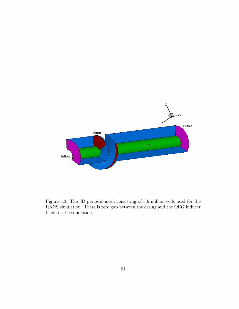
4.3 The 3D periodic mesh consisting of 3.6 million cells used for theRANS simulation. There is zero gap between the casing and theOEG inducer blade in the simulation. . . . . . . . . . . . . . 61
4.4 The circulation distribution on the OEG inducer blade from thepresent panel method at advance coeffficient J = 0.2652. Thereare 120×20 panels on the blade, 90×20 panels on the hub and200× 20 panels on the casing. . . . . . . . . . . . . . . . . . . 62
4.5 Comparison of pressure distributions on the OEG inducer bladefrom the present panel method and FLUENT viscous run atadvance coefficient J = 0.2652 and radius of 0.43. There are120 × 20 panels on the blade, 90 × 20 panels on the hub and160 × 20 panels on the casing. The 3D periodic mesh has 2.3million cells. . . . . . . . . . . . . . . . . . . . . . . . . . . . . 63
4.6 Comparison of pressure distributions on the OEG inducer bladefrom the present panel method and FLUENT viscous run atadvance coefficient J = 0.2652 and radius of 0.70. There are120 × 20 panels on the blade, 90 × 20 panels on the hub and200 × 20 panels on the casing. The 3D periodic mesh has 2.3million cells. . . . . . . . . . . . . . . . . . . . . . . . . . . . . 64
4.7 Comparison of pressure distributions on the OEG inducer bladefrom the present panel method and FLUENT viscous run atadvance coefficient J = 0.2652 and radius of 0.97. There are120 × 20 panels on the blade, 90 × 20 panels on the hub and200 × 20 panels on the casing. The 3D periodic mesh has 2.3million cells. . . . . . . . . . . . . . . . . . . . . . . . . . . . . 65
xv

4.8 The fabricated inducer from Scheer et al. (1970). The operatingconditions are at flow coefficient of 0.0084 which correspondsto an advance coefficient J = 0.2652, 100% speed and a netpositive suction head (NPSH) of 32.3 m. . . . . . . . . . . . . 66
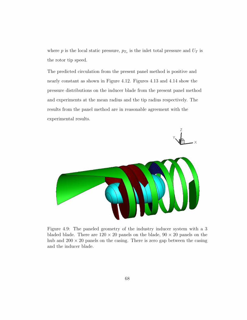
4.9 The paneled geometry of the industry inducer system with a 3bladed blade. There are 120× 20 panels on the blade, 90× 20panels on the hub and 200× 20 panels on the casing. There iszero gap between the casing and the inducer blade. . . . . . . 68
4.10 The original industry inducer blade geometry is essentially con-stant thickness which suddenly tapers off at the leading andtrailing edges. . . . . . . . . . . . . . . . . . . . . . . . . . . 69
4.11 The new blade section of the industry inducer with no camberand constant thickness everywhere except at the leading andtrailing edge where they are closed with elliptic ends. Hence itis a constant thickness blade for 97 % of the chord length. . . 69
4.12 The circulation distribution on the industry inducer blade fromthe present panel method at advance coefficient J = 0.2652.Thereare 120×20 panels on the blade, 90×20 panels on the hub and200× 20 panels on the casing. . . . . . . . . . . . . . . . . . . 70
4.13 Comparison of pressure distributions on the industry inducerblade from the present panel method and experimental resultsat advance coeffficient J = 0.2652 and mean radius of 0.68.There are 120 × 20 panels on the blade, 90 × 20 panels on thehub and 200×20 panels on the casing.The experimental resultsare obtained from Scheer et al. (1970). . . . . . . . . . . . . . 71
4.14 Comparison of pressure distributions on the industry inducerblade from the present panel method and experimental resultsat advance coefficient J = 0.2652 and tip radius of 0.94. Thereare 120 × 20 panels on the blade, 90 × 20 panels on the huband 200× 20 panels on the casing.The experimental results areobtained from Scheer et al. (1970). . . . . . . . . . . . . . . . 72
4.15 The predicted circulation distribution on the industry inducerblade from the cavitating and fully wetted simulations using thepresent panel method at an advance coeffficient J = 0.2652 andσ = 2.8977 .There are 120 × 20 panels on the blade, 90 × 20panels on the hub and 200× 20 panels on the casing. . . . . . 74
4.16 Comparison of pressure distributions on the industry inducerblade from the cavitating and fully wetted analysis using thepresent panel method at an advance coefficient J = 0.2652,σ = 2.8977 and mean radius of 0.68. There are 120× 20 panelson the blade, 90× 20 panels on the hub and 200× 20 panels onthe casing. . . . . . . . . . . . . . . . . . . . . . . . . . . . . . 75
xvi
4.17 Comparison of pressure distributions on the industry inducerblade from the cavitating and fully wetted analysis using thepresent panel method at an advance coefficient J = 0.2652,σ = 2.8977 and tip radius of 0.94. There are 120 × 20 panelson the blade, 90× 20 panels on the hub and 200× 20 panels onthe casing. . . . . . . . . . . . . . . . . . . . . . . . . . . . . . 76
4.18 The cavities at the leading edge on the suction side of the indus-try inducer blade from the present panel method at J = 0.2652and σ = 2.8977 . There are 120×20 panels on the blade, 90×20panels on the hub and 200× 20 panels on the casing. . . . . . 77
xvii

Nomenclature
Latin Symbols
Cf skin-friction coefficient Cf = τwall/(0.5ρU2)
Cp pressure coefficient, Cp = (p− po)/(0.5ρn2D2)
D propeller diameter, D = 2R
fmax/C maximum camber to chord ratio
FnD Froude number based on VA, FnD = VA/√gD
Fr Froude number based on n, Fr = n2D/g
g gravitational acceleration
G Green’s function
hgap gap size
J advance ratio based on Vs, J = Vs/(nD)
KQ torque coefficient, KQ = Q/(ρn2D5)
KT thrust coefficient, KT = T/(ρn2D4)
n propeller rotational frequency (rps)
p pressure
po pressure far upstream
pv vapor pressure of the fluid
P pitch angle
xviii

q total velocity
Q torque
U in local inflow velocity (in the propeller fixed system)
u Perturbation velocity
R propeller radius
Re Reynolds number
SR rotor surface
SRW rotor wake surface
SHC hub and casing surfaces
SS stator surface
SSW stator wake surface
T thrust
tmax/C maximum thickness to chord ratio
τwall wall shear stress
VA advance speed of propeller
uτ wall shear velocity, uτ =√τwall/ρ
X, Y, Z propeller fixed coordinates
XS, YS, ZS ship fixed coordinates
y+ non-dimensional wall distance, y+ = uτyν
xix

Greek Symbols
α angle of attack
Γ circulation
∆t time step size
ν kinematic viscosity of water
φ perturbation potential
Φ total potential
∆φTE potential jump at the trailing edge of the blade
∆φW potential jump across the shed wake sheet of the blade
ρ fluid density
σn cavitation number based on n, σn = (po − pv)/(0.5ρn2D2)
σv cavitation number based on VA, σv = (po − pv)/(0.5ρV 2A)
ω propeller angular velocity
xx

Uppercase Abbreviations
2D two dimensional
3D three dimensional
BEM Boundary Element Method
CPU Central processing unit
ITTC International Towing Tank Conference
MIT Massachusetts Institute of Technology
NACA National Advisory Committee for Aeronautics
ONR-AXWJ Office of Naval Research Axial Water-jet
RANS Reynolds-Averaged Navier Stokes
SIMPLEC Semi-Implicit Method for Pressure
Linked Equations-Consistent scheme
VLM Vortex-Lattice Method
Computer Program Names
FLUENT A commercial RANS solver
PROPCAV A cavitating propeller potential flow solver based on BEM
XFOIL A 2D integral boundary layer analysis code
xxi

Chapter 1
Introduction
1.1 Introduction
A water-jet is a marine propulsion system that produces a jet of rapid
water behind the ship for high-speed propulsion. The first working water-jet
system was developed by Secondo Campini in Venice in 1931. Bill Hamilton,
a New Zealand engineer built the first commercial water-jet propulsion system
in 1954.
Initially water-jets were limited to high speed pleasure boats such as
jet skis and jet boats. However the increasing demand for high-speed ships
in recent years has led to the adoption of water-jet propulsion systems for
commercial and naval vessels. Ships fitted with water-jet propulsion systems
can achieve speeds up to 40 knots, even with a conventional hull. Luxury high
speed motor yachts have achieved speeds above 65 knots, which is about 120
km/h. Figure 1.1 shows a marine vessel employing water-jet propulsion.
The nonexistence of appurtenances such as shafts, ducts and rudders
below the waterline reduces the ship resistance and makes water-jets the cho-
sen method for shallow water maneuvering. The damages from sizable debris
to the propeller can be reduced inside the water-jet propulsion system. The
1

Figure 1.1: A high-speed police vessel utilizing water-jet propulsion (source:http://www.hamjet.co.nz/model range).
occurrence of cavitation can also be reduced at lower ship speeds as compared
to the open propeller. However cavitation can still occur at higher ship speeds
and lead to thrust breakdown. The complicated geometry of the water-jet
propulsion system, the inescapable cavitation due to pressure drops at high
ship speeds and the innate unsteadiness of the rotor-stator interaction culmi-
nates in making the research and study of viscous flows in water-jet systems
difficult. Figures 1.2 and 1.3 show the geometry configuration of a typical
water-jet propulsion system.
1.2 Literature Review
Several numerical and experimental approaches have been developed
and applied to analyse the water-jet propulsion system over the past two
decades. An extensive study of the problems confronted in designing and
2
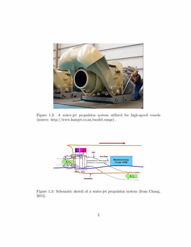
Figure 1.2: A water-jet propulsion system utilized for high-speed vessels(source: http://www.hamjet.co.nz/model range) .
Figure 1.3: Schematic sketch of a water-jet propulsion system (from Chang,2012).
3

calculating the hydrodynamic parameters of water-jet propulsion systems was
carried out by Kerwin (2006). The International Towing Tank Conference pa-
per (2008) presents a meticulous analysis and characterization of state of the
art water-jet propulsion systems. Reynolds Averaged Navier-Stokes (RANS)
schemes have been utilized with growing success for the analysis of internal
flows in water-jet propulsion systems. Kim et al. (2002) used an in-house
RANS code to compute a full water-jet system (inlet duct, rotor, stator and
outlet nozzle) for a tracked vehicle. The authors used the code to look at
some differences between two pump systems and to propose design changes to
optimize the flow through the system. A RANS scheme employing a shifting,
non-orthogonal grid was utilized by Chun et al. (2002) to study the rotor-
stator interaction . The rotor was analyzed in an unsteady manner and the
effect of the stator was considered in a circumferentially averaged manner.
Brewton et al. (2006) employed a RANS scheme with the mixing plane model
and analyzed the rotor-stator interaction in a water-jet propulsion system in
a time-averaged manner. A RANS scheme with multiphase modeling ability
was employed by Lindau et al. (2009; 2011). The authors utilized a power
iteration algorithm to analyze a water-jet propulsion system at different flow
coefficients and predict the thrust/torque breakdown due to cavitation.
The design and calculation of hydrodynamic performance parameters
of water-jet propulsion systems have also been carried out using a transitional
approach which couples a potential flow scheme with a RANS scheme. A
vortex lattice scheme combined with either an Euler equation solver or a RANS
4

scheme was utilized by Kerwin et al. (1997) and Taylor et al. (1998) to consider
the impact of the hull and to study the entire flow in a water-jet propulsion
system. A potential flow panel method was employed by Kinnas, Chang et
al.(2007, 2010, 2012) to calculate the hydrodynamic performance parameters of
a water-jet propulsion system. The rotor- stator interaction was accomplished
using an iterative procedure which considers the effect of circumferentially
averaged induced potentials between the rotor and the stator. Sun and Kinnas
et al. (2006) and Kinnas et al. (2007) have analyzed the effects of viscous flow
through ducted propellers and the ONR-AXWJ1 water-jet propulsion system
by coupling the potential flow panel method with the boundary layer method
XFOIL (Drela, 1989). This numerical approach is capable of capturing the
repercussions of the boundary layer on the blade cavities.
1.3 Objectives
• The objective of this thesis is to refine and enhance a potential flow
solver PROPCAV, based on the panel method by Kinnas and Fine
(1993), and to analyze the steady fully-wetted performance of water-jet
propulsion systems.
• The present panel method will be used to evaluate the hydrodynamic
performance characteristics of the water-jet propulsion system and the
results will be compared with RANS calculations.
• The present panel method will utilize a numerical scheme to evaluate
5

the dipole and source influence coefficients of non-planar hyperboloid
surface panels more accurately.
• The numerical panel method will also be extended to analyze the
performance of an inducer as further demonstration of its applicability.
1.4 Organization
This thesis is organized into five chapters.
Chapter 1 contains the literature review, the objectives and the organization
of this study.
Chapter 2 explains the methodology, governing equations and boundary
conditions utilized in the present numerical method.
Chapter 3 describes the application of the numerical panel method for the
analysis and hydrodynamic performance prediction of water-jet propulsion
systems.
Chapter 4 describes the extension of the numerical panel method to study
rocket engine inducers.
Chapter 5 presents the conclusions and the recommendations for future work.
6

Chapter 2
Methodology
A numerical panel method is refined and enhanced to analyze water-jet
propulsion systems. This chapter describes the governing equations, the
numerical method and the boundary conditions involved in solving inviscid
wetted flows inside a water-jet propulsion system.
2.1 Governing Equations
The typical configuration of a water-jet propulsion system along with its
coordinate systems is shown in Figure 2.1. The ship fixed coordinate system
is denoted by (Xs, Ys, Zs) and (X, Y, Z) represents the propeller fixed
coordinate system. The inflow ~U specified at the water-jet inlet is defined in
a ship fixed coordinate system and is assumed to be uniform for steady
problems.
The rotor blades rotate with a constant angular velocity vector ~ω. The stator
blades do not rotate and are fixed with respect to the propeller coordinate
system ~X. Therefore the total inflow velocity ~Vin in the propeller fixed
coordinate system can be expressed as ~Vin = ~U + ~ω × ~X for the rotor and
~Vin = ~U for the stator. The velocity field for an inviscid, irrotational and
7

incompressible flow, in the rotating frame of reference, is expressed as
~qt(x, y, z) = ~Vin(x, y, z) +∇φ(x, y, z) (2.1)
where ~qt(x, y, z) is the total velocity at any point inside the fluid domain, φ is
the perturbation potential which satisfies the Laplace equation ∇2φ = 0.
The perturbation potential φ(x, y, z) at any point on the rotor (SR),stator
(SS), hub (SH) and casing (SC) surfaces has to satisfy the Green’s third
identity as given in equation 2.2.
2πφ =
∫SR
[φq∂G(p; q)
∂nq−G(p; q)
∂φ
∂nq
]ds
+
∫SRW
4φRW∂G(p; q)
∂nqds
+
∫SS
[φq∂G(p; q)
∂nq−G(p; q)
∂φ
∂nq
]ds
+
∫SSW
4φSW∂G(p; q)
∂nqds
+
∫SHC
[φq∂G(p; q)
∂nq−G(p; q)
∂φ
∂nq
]ds
(2.2)
where p and q correspond to the variable point and the field point
respectively, G(p : q) = 1R(p;q)
is the Green function and R(p; q) is the
distance between the field point p and the variable point q,n indicates the
normal direction pointing into the flow field, 4φRW and 4φSW are the
potential jumps across the trailing wake sheets shed from the rotor and the
stator blade trailing edge respectively.
The flow inside a water-jet propulsion system is simulated through an
iterative procedure which solves the rotor problem and the stator problem
8

Figure 2.1: Coordinate systems utilized for the analysis of a water-jet propul-sion system (Kinnas et al. 2012)
separately and accounts for the rotor-stator interaction by considering the
circumferentially averaged effects of each component on the other. A fully
unsteady simulation as given in Tian (2013) needs to be performed in order
to totally capture the interaction between the rotor and the stator. The
computational resources required for such a simulation is exceedingly
expensive.
The rotor-stator interaction is carried out via induced velocities in the
present method. Hence the numerical method is known as the induced
velocity method. In addition, the rotor is solved with respect to the rotating
coordinate system and the stator is solved with respect to the ship fixed
coordinate system. Figure 2.2 is the diagrammatic outline of the rotor and
stator problem, the rotor only problem, and the stator only problem
respectively. More details on the induced velocity method for the rotor-stator
9

interaction can be found in Chang (2012).
2.2 Numerical Method
The integral equations for the rotor and stator problems and the calculation
of the circumferentially averaged induced velocities are presented in this
section.
2.2.1 Rotor only problem
The integral equation for the rotor problem is given as
2πφ =
∫SR
[φq∂G(p; q)
∂nq−G(p; q)
∂φ
∂nq
]ds
+
∫SRW
4φRW∂G(p; q)
∂nqds
+
∫SHC
[φq∂G(p; q)
∂nq−G(p; q)
∂φ
∂nq
]ds
(2.3)
where the source strength ∂φ/∂n is modified as
∂φ
∂n= −(~Vin + ~uRS).~n (2.4)
where ~uRS is the circumferentially averaged velocities on the rotor, hub and
casing surfaces induced by the stator which are evaluated from the following
integral equation
4π~uRS =
∫SS
[φq∇
∂G(p; q)
∂nq−∇G(p; q)
∂φ
∂nq
]ds
+
∫SSW
4φSW∇∂G(p; q)
∂nqds
(2.5)
More information on calculating the induced potentials and velocities can be
obtained from Newman (1986).
10
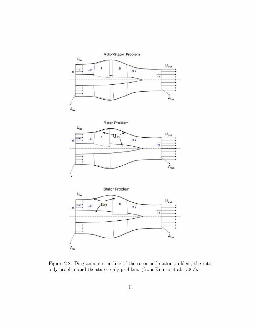
Figure 2.2: Diagrammatic outline of the rotor and stator problem, the rotoronly problem and the stator only problem. (from Kinnas et al., 2007).
11

2.2.2 Stator only problem
The integral equation for the stator problem is given as
2πφ =
∫SS
[φq∂G(p; q)
∂nq−G(p; q)
∂φ
∂nq
]ds
+
∫SSW
4φRW∂G(p; q)
∂nqds
+
∫SHC
[φq∂G(p; q)
∂nq−G(p; q)
∂φ
∂nq
]ds
(2.6)
where the source strength ∂φ/∂n is modified as
∂φ
∂n= −(~Vin + ~uSR).~n (2.7)
where ~uSR is the circumferentially averaged velocities on the stator, hub and
casing surfaces induced by the stator which are evaluated from the following
integral equation
4π~uSR =
∫SR
[φq∇
∂G(p; q)
∂nq−∇G(p; q)
∂φ
∂nq
]ds
+
∫SRW
4φSW∇∂G(p; q)
∂nqds
(2.8)
2.3 Boundary conditions
The following boundary conditions need to be satisfied for analyzing the
water-jet system. The kinematic boundary condition on the rotor, stator,
hub and casing surfaces requires that the flow must be tangent to the body
surfaces.
∂φ
∂n= −~Vin.~n (2.9)
12

The Kutta condition ensures that the velocities at the trailing edge of the
blade are finite. An iterative pressure Kutta condition is applied to ensure
that the pressures on the pressure side and suction side of the blade trailing
edge are equal. Further details are given in Kinnas and Hsin (1992).
The flow field is assumed to equal the inflow velocity at the inlet of the
water-jet system.
∂φ
∂n
∣∣∣∣inflow
= 0 (2.10)
It should be noted that the inlet panels of the water-jet are removed and the
perturbation potentials are set to be zero on those panels to obtain an
unique solution of the internal boundary value problem.
The conservation of mass law must be fulfilled at the water-jet outlet. Hence
we obtain
Vin · Ain = Vout · Aout (2.11)
where Vin is the inlet velocity, Ain and Aout are the water-jet inflow and
outflow surface areas respectively.
2.4 Numerical evaluation of influence coefficients
This section describes the evaluation of dipole and source influence
coefficents using numerical integration for hyperboloid panels. The numerical
integration is accomplished using Gauss quadrature.
13

2.4.1 Gauss quadrature
The Green’s integral equation 2.2 can be written in the following discretized
form on all the panels, with the Green function G(p : q) = 1R(p;q)
and
∂φ∂nq
= −~Vin.~nq, ∑k
Alkφk =∑k
(−~Vin.~nk)Blk (2.12)
The dipole influence coefficient Alk is given as
Alk =
∫ ∫Sk
~nk · ∇(1
rlk)dsk (2.13)
and the source influence coefficent Blk is given as
Blk =
∫ ∫Sk
1
rlkdsk (2.14)
where ~nk represents the normal vector, rlk represents the distance to the
control point and dsk represents the elemental surface area.
The discretized form of the dipole (Alk) and source (Blk) influence
coefficients associated with a panel is
A =n∑i=1
n∑j=1
~nij · ∇(1
rij)wij∆s (2.15)
B =n∑i=1
n∑j=1
1
rijwij∆s (2.16)
where (i, j) represents the Gaussian point on the panel, ~nij represents the
normal vector, n represents the number of Gaussian points on the panel and
rij represents the distance to the control point as shown in Figure 2.3. Here
14

Figure 2.3: A panel discretized with Gaussian points to evaluate the influencecoefficients numerically. The interior of the panel is discretized with n = 3Gaussian points.
wij represents the weight for each Gaussian point and the surface area
∆s = ∆x∆y|J | where J is the Jacobian.
The present panel method uses n = 8 Gaussian points to discretize the panel.
We have also tried n = 4 and n = 16 Gaussian points to discretize the panel.
The time taken to complete 104 calculations for a panel discretized with
n = 4 , n = 8 and n = 16 Gaussian points are 7s, 10s and 18s respectively.
Hence we decided to select n = 8 Gaussian points to provide a balance
between accuracy and speedy computation.
2.4.2 Non-planar quadrilateral
In order to validate the Gauss quadrature scheme, we use it to calculate the
dipole and source influence coefficients of a non-planar quadrilateral as
15

shown in Figure 2.4. The control point is moved along the z axis.
Figure 2.4: The non-planar quadrilateral considered for evaluating the influ-ence coefficients. The control point is moved along the z axis.
The relative error in calculating the dipole and source influence coefficients
are shown in Figures 2.5 and 2.6 respectively. The relative error is defined as
relative error = (|vnumerical − vexact|
|vexact|) (2.17)
The exact value is obtained using MATLAB to compute the integrals.
It is observed that the relative error in evaluating the dipole influence
coefficient by Gauss quadrature scheme increases rapidly as the control point
is moved very close to the panel. This is because the numerical scheme in its
present form cannot resolve the singularity in A as rij → 0 . This error is
mitigated by evaluating the dipole influence coefficients of a hyperboloid
16

Figure 2.5: Relative error in calculating the dipole influence coefficient of thenon-planar quadrilateral shown in Figure 2.4. The control point is movedalong the z axis.
Figure 2.6: Relative error in calculating the source influence coefficient of thenon-planar quadrilateral shown in Figure 2.4. The control point is movedalong the z axis.
17

panel using the approach developed by Morino, Chen and Suciu (1975).
However this scheme is valid only for control points very close to the panel.
Henceforth for the calculation of the dipole influence coefficients we will use
the Morino formula for control points very close to the panel (like
self-influence coefficients) and Gauss quadrature for control points farther
away.
2.4.3 Casing only problem
After using the Gauss quadrature numerical scheme to analyze a single
non-planar panel, we move on to a simplified case, considering the casing
only problem of a water-jet propulsion system. The casing selected was the
casing of a water-jet propulsion system as shown in Figure 2.8.
The paneling on the casing of the water-jet system follows the pitch angle
(P ) of the rotor blade. The pitch angle of a rotor blade is the angle between
the chord line and a reference plane determined by the rotor hub or the plane
of rotation as shown in Figure 2.7. For low pitch rotor blades we have highly
skewed panels on the casing. The planar method used to evaluate the
influence coefficients is RPAN (Newman 1986), which handles non-planar
panels as planar panels resulting from the projection of the non-planar panel
on the midpoint plane. This method requires a large number of panels to
properly evaluate the dipole and source influence coefficients for low pitch
cases. However using hyperboloid panels and the non-planar numerical
method allows us to significantly reduce the number of panels used to
18

discretize the surface of the casing.
Figure 2.7: The pitch angle of a rotor blade is the angle between the chord lineand a reference plane (source: http://www.allstar.fiu.edu/aero/flight63.htm).
In the study, the pitch angle considered is 80o as shown in Figure 2.8. The
total number of panels used to discretize the casing is 4000. The number of
axial elements is 240 and the number of circumferential elements is 40 on the
casing. The results for P = 80o case given in Figure 2.9 are also compared
with the results for P = 0o case given in Figure 2.10 where both the planar
and non-planar methods work very well. We observe that the non-planar
method works admirably well for P = 80o case while the planar method fails
for the same case.
19

Figure 2.8: Paneling on the water-jet casing for P = 80o case. The totalnumber of panels used to discretize the casing is 4000.The number of axialelements is 240 and the number of circumferential elements is 40 on the casing.
20

Figure 2.9: Pressure distribution on the casing for P = 80o case . The totalnumber of panels used to discretize the casing is 4000.The number of axialelements is 240 and the number of circumferential elements is 40 on the casing.
21

Figure 2.10: Pressure distribution on the casing for P = 0o case. The totalnumber of panels used to discretize the casing is 4000.The number of axialelements is 240 and the number of circumferential elements is 40 on the casing.
22

Chapter 3
Numerical Analysis of Water-jets
This chapter presents the numerical analysis of axial flow water-jet pumps
using the present panel method. The present study considers water-jets
subject to a uniform inflow and only the steady simulations are considered
here. The interaction between the rotor and the stator is carried out by
applying the induced velocity method. The design advance ratio is 1.19 and
the rotational frequency is 1400 rpm for the fully wetted condition. The
numerical results from the present panel method are compared with
Reynolds Averaged Navier-Stokes (RANS) calculations using FLUENT.
3.1 Nondimensional Coefficients
The nondimensional coefficients utilized in this thesis are explained below.
The circulation Γ is given from Kinnas (2012)
Γ =∆φ
2πR√U2in + (0.7nπD)2
(3.1)
where 4φ indicates the potential jump at trailing edge of the rotor blade in
the present method. The advance ratio Js and the Reynolds number Re are
also given as:
Js =UinnD
, Re =UinR
ν(3.2)
23

where Uin is the flow velocity at the inlet boundary, R represents the radius
of the rotor and νdenotes the kinematic viscosity.The pressure coefficient Cp
used in the present method is defined as follows
Cp =p− po
0.5ρn2D2(3.3)
where po is the far upstream pressure on the shaft axis.
3.2 Rotor only Case
Two different cases are considered in this section for the rotor only analysis.
The only difference between these two cases is in the geometry of the casing.
First we will present the results obtained by analyzing the water-jet rotor
system with a cylindrical casing. Then we will move on to the more realistic
case of the Office of Naval Research Axial Water-jet (ONR-AXWJ2) rotor
pump.
3.2.1 Rotor with cylindrical casing
The paneled geometry of the rotor analysed with the present numerical
method is shown in Figure 3.1. The rotor blade has the NACA-16 thickness
form and a sharp trailing edge. The present method takes 10 minutes for a
fully-wetted analysis by using 120× 40 panels on the blade, 90× 20 panels
on the hub and 200× 20 panels on the casing. The first number in the legend
120× 40 denotes the number of panels in the chord-wise or axial direction
and the second number denotes the number of elements in the span-wise
24
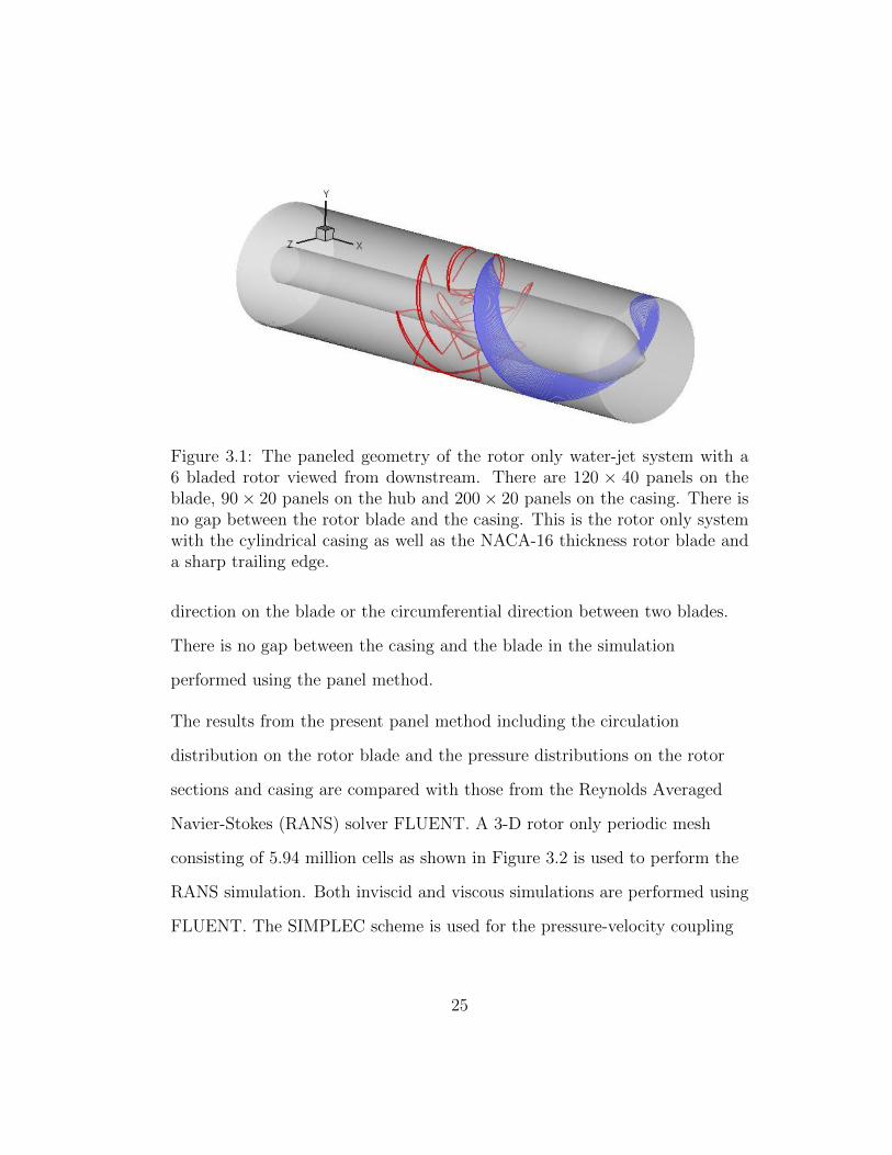
Figure 3.1: The paneled geometry of the rotor only water-jet system with a6 bladed rotor viewed from downstream. There are 120 × 40 panels on theblade, 90× 20 panels on the hub and 200× 20 panels on the casing. There isno gap between the rotor blade and the casing. This is the rotor only systemwith the cylindrical casing as well as the NACA-16 thickness rotor blade anda sharp trailing edge.
direction on the blade or the circumferential direction between two blades.
There is no gap between the casing and the blade in the simulation
performed using the panel method.
The results from the present panel method including the circulation
distribution on the rotor blade and the pressure distributions on the rotor
sections and casing are compared with those from the Reynolds Averaged
Navier-Stokes (RANS) solver FLUENT. A 3-D rotor only periodic mesh
consisting of 5.94 million cells as shown in Figure 3.2 is used to perform the
RANS simulation. Both inviscid and viscous simulations are performed using
FLUENT. The SIMPLEC scheme is used for the pressure-velocity coupling
25
in the simulation. There is no gap between the casing and the blade in the
periodic mesh. The k − ω SST model is used for the viscous simulation. The
moving wall boundary condition is used on the casing and the hub. The y+
varies from 50 to 400 on the hub and from 40 to 180 on the casing. The
simulations take about 8 hours by using 16 CPUs to complete 20,000
iterations on a cluster with 2.43 GHZ quad-core 64-bit Intel Xeon processors
and 16 GB of RAM.
Figure 3.3 shows the circulation distributions on the rotor blade from the
present panel method PROPCAV and the FLUENT inviscid run. Figures 3.4
to 3.6 show the pressure distributions on the rotor blade from the present
panel method and FLUENT viscous and inviscid runs at different radii. The
two Cp(mean) curves presented in Figure 3.7 are obtained by
circumferentially averaging pressures over all the strips on the casing surface
from the 3-D FLUENT simulation and those from the present panel method.
Figure 3.7 shows that the pressure rise on the casing surface from the present
panel method and the viscous FLUENT simulation are in good agreement.
26

Inflow
Casing
Rotor
Periodic boundary
Outlet
Figure 3.2: The 3D periodic mesh consisting of 5.94 million cells used forthe RANS simulation. There is zero gap between the casing and the rotorblade. This is the rotor only system with the cylindrical casing as well as theNACA-16 thickness rotor blade and a sharp trailing edge.
27

Figure 3.3: Comparison of circulation distributions on the rotor blade fromthe present panel method and FLUENT inviscid run at advance coefficientJ = 1.19.There are 120 × 40 panels on the blade, 90 × 20 panels on the huband 200 × 20 panels on the casing. The 3D periodic mesh has 5.94 millioncells. This is the rotor only system with the cylindrical casing as well as theNACA-16 thickness rotor blade and a sharp trailing edge.
28

Figure 3.4: Comparison of pressure distributions on the rotor blade from thepresent panel method and FLUENT inviscid and viscous runs at advance co-efficient J = 1.19 and radius of 0.55. There are 120× 40 panels on the blade,90× 20 panels on the hub and 200× 20 panels on the casing. The 3D periodicmesh has 5.94 million cells. This is the rotor only system with the cylindricalcasing as well as the NACA-16 thickness rotor blade and a sharp trailing edge.
29

Figure 3.5: Comparison of pressure distributions on the rotor blade from thepresent panel method and FLUENT inviscid and viscous runs at advance co-efficient J = 1.19 and radius of 0.70. There are 120× 40 panels on the blade,90× 20 panels on the hub and 200× 20 panels on the casing. The 3D periodicmesh has 5.94 million cells. This is the rotor only system with the cylindricalcasing as well as the NACA-16 thickness rotor blade and a sharp trailing edge.
30

Figure 3.6: Comparison of pressure distributions on the rotor blade from thepresent panel method and FLUENT inviscid and viscous runs at advance co-efficient J = 1.19 and radius of 0.95. There are 120× 40 panels on the blade,90× 20 panels on the hub and 200× 20 panels on the casing. The 3D periodicmesh has 5.94 million cells. This is the rotor only system with the cylindricalcasing as well as the NACA-16 thickness rotor blade and a sharp trailing edge.
31

Figure 3.7: Comparison of circumferentially averaged pressure distributionson the casing surface from the present panel method and FLUENT viscousrun at advance coefficient J = 1.19. There are 120 × 40 panels on the blade,90× 20 panels on the hub and 200× 20 panels on the casing. The 3D periodicmesh has 5.94 million cells. This is the rotor only system with the cylindricalcasing as well as the NACA-16 thickness rotor blade and a sharp trailing edge.
32

Figure 3.8: The paneled geometry of the ONR-AXWJ2 rotor only system withthe 6 bladed rotor viewed from downstream. There are 120× 40 panels on theblade, 90× 20 panels on the hub and 160× 20 panels on the casing. There isno gap between the casing and the blade. This is the ONR-AXWJ2 rotor onlysystem with the NACA-16 thickness rotor blade and a sharp trailing edge.
3.2.2 ONR-AXWJ2 Rotor Case
The paneled geometry of the rotor analysed with the present numerical
method is shown in Figure 3.8. The rotor blade has the NACA-16 thickness
form and a sharp trailing edge. The present method takes 8 minutes for a
fully-wetted analysis by using 120× 40 panels on the blade, 90× 20 panels
on the hub and 160× 20 panels on the casing. There is no gap between the
casing and the blade in the simulation performed using the panel method.
The results from the present panel method including the pressure
distributions on the rotor sections and the casing are compared with those
from the Reynolds Averaged Navier-Stokes (RANS) solver FLUENT. A 3-D
rotor only periodic mesh consisting of 2.3 million cells as shown in Figure 3.9
is used to perform the RANS simulation. We have only performed viscous
33
simulations in FLUENT using the created mesh. The SIMPLEC scheme is
used for the pressure-velocity coupling in the simulation. There is a gap of
0.33% between the casing and the blade in the periodic mesh. The k − ω
SST model is used for the viscous simulation. The stationary wall boundary
condition is used on the casing and the moving wall boundary condition on
the hub. The y+ varies from 50 to 420 on the hub and from 40 to 190 on the
casing. There are 10 layers in the tip gap region of the mesh. The
simulations take about 10 hours by using 16 CPUs to complete 20,000
iterations on a cluster with 2.43 GHZ quad-core 64-bit Intel Xeon processors
and 16 GB of RAM.
Figure 3.10 shows the circulation distributions on the rotor blade from the
present panel method. Figures 3.11 to 3.13 show the pressure distributions
on the rotor blade from the present panel method and FLUENT viscous and
inviscid runs at different radii.
The two Cp(mean) curves presented in Figure 3.14 are obtained by
circumferentially averaging pressures over all the strips on the casing surface
from the 3-D FLUENT simulation and those from the present panel method.
Figure 3.14 shows that the pressure rise on the casing surface from the
present panel method and the viscous FLUENT simulation are in good
agreement.
34

Figure 3.9: The 3D periodic mesh consisting of 2.3 million cells used for theRANS simulation. There is 0.33% gap between the casing and the rotor blade.This is the ONR-AXWJ2 rotor only system with the NACA-16 thickness bladeand a sharp trailing edge.
35

Figure 3.10: The circulation distribution on the rotor blade from the presentpanel method at advance coefficient J = 1.19.There are 120×40 panels on theblade, 90 × 20 panels on the hub and 160 × 20 panels on the casing. This isthe ONR-AXWJ2 rotor only system with the NACA-16 thickness rotor bladeand a sharp trailing edge.
36

Figure 3.11: Comparison of pressure distributions on the rotor blade fromthe present panel method and FLUENT viscous run at advance coefficientJ = 1.19 and radius of 0.55. There are 120× 40 panels on the blade, 90× 20panels on the hub and 160 × 20 panels on the casing. The 3D periodic meshhas 2.3 million cells. This is the ONR-AXWJ2 rotor only system with theNACA-16 thickness rotor blade and a sharp trailing edge.
37

Figure 3.12: Comparison of pressure distributions on the rotor blade fromthe present panel method and FLUENT viscous run at advance coefficientJ = 1.19 and radius of 0.70. There are 120× 40 panels on the blade, 90× 20panels on the hub and 160 × 20 panels on the casing. The 3D periodic meshhas 2.3 million cells. This is the ONR-AXWJ2 rotor only system with theNACA-16 thickness rotor blade and a sharp trailing edge.
38
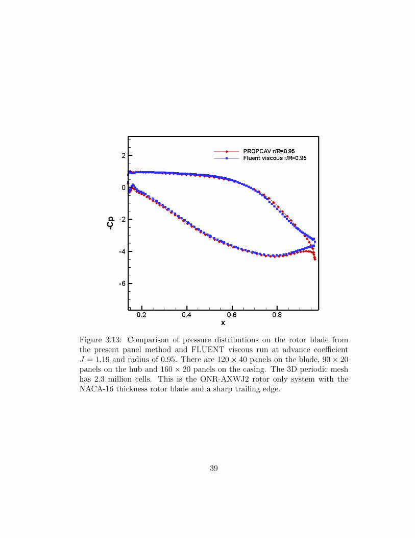
Figure 3.13: Comparison of pressure distributions on the rotor blade fromthe present panel method and FLUENT viscous run at advance coefficientJ = 1.19 and radius of 0.95. There are 120× 40 panels on the blade, 90× 20panels on the hub and 160 × 20 panels on the casing. The 3D periodic meshhas 2.3 million cells. This is the ONR-AXWJ2 rotor only system with theNACA-16 thickness rotor blade and a sharp trailing edge.
39

Figure 3.14: Comparison of circumferentially averaged pressure distributionson the casing surface from the present panel method and FLUENT viscousrun at advance coefficient J = 1.19. There are 120 × 40 panels on the blade,90× 20 panels on the hub and 160× 20 panels on the casing. The 3D periodicmesh has 2.3million cells. This is the ONR-AXWJ2 rotor only system withthe NACA-16 thickness rotor blade and a sharp trailing edge.
40

3.3 Stator only Case
The designed stator is analyzed separately while enclosed in a cylindrical
casing. The paneled geometry of the stator analysed with the present
numerical method is shown in Figure 3.15.The stator is stationary and does
not rotate. The present method takes 1 minute for a fully-wetted analysis by
using 100× 40 panels on the blade, 90× 20 panels on the hub and 200× 20
panels on the casing. The first number in the legend 100× 40 denotes the
number of panels in the chord-wise or axial direction and the second number
denotes the number of elements in the span-wise direction on the blade or
the circumferential direction between two blades. There is no gap between
the casing and the stator blade in the simulation performed using the panel
method.
The pressure distributions on the stator sections from the present panel
method are compared with those from the Reynolds Averaged Navier-Stokes
(RANS) solver FLUENT. A 3-D stator only periodic mesh consisting of 1.6
million cells as shown in Figure 3.16 is used to perform the RANS
simulation. We have only performed inviscid simulations in FLUENT using
the created mesh. The SIMPLEC scheme is used for the pressure-velocity
coupling in the simulation. There is no gap between the casing and the blade
in the periodic mesh. The moving wall boundary condition is used on the
casing and the hub. The simulations take about 4 hours by using 16 CPUs to
complete 20,000 iterations on a cluster with 2.43 GHZ quad-core 64-bit Intel
Xeon processors and 16 GB of RAM.
41

Figures 3.17 to 3.18 show the pressure distributions on the stator blade from
the present panel method and FLUENT inviscid runs at different radii. The
results from the panel method are in good agreement with the RANS inviscid
calculations. The circulation distribution on the stator blade from the
present panel method is given in 3.19.
42

Figure 3.15: The paneled geometry of the stator only system with a 8 bladedstator. There are 100× 40 panels on the blade, 90× 20 panels on the hub and200 × 20 panels on the casing. There is no gap between the casing and theblade. This is the designed stator only system with the cylindrical casing.
Figure 3.16: The 3D periodic mesh consisting of1.6 million cells used for theRANS simulation. There is zero gap between the casing and the stator blade.This is the designed stator only system with the cylindrical casing.
43

Figure 3.17: Comparison of pressure distributions on the stator blade fromthe present panel method and FLUENT inviscid run at advance coefficientJ = 1.00 and radius of 0.35. There are 100× 40 panels on the blade, 90× 20panels on the hub and 200×20 panels on the casing. The 3D periodic mesh has1.6 million cells. This is the designed stator only system with the cylindricalcasing.
44

Figure 3.18: Comparison of pressure distributions on the stator blade fromthe present panel method and FLUENT inviscid run at advance coefficientJ = 1.00 and radius of 0.90. There are 100× 40 panels on the blade, 90× 20panels on the hub and 200×20 panels on the casing. The 3D periodic mesh has1.6 million cells. This is the designed stator only system with the cylindricalcasing.
45
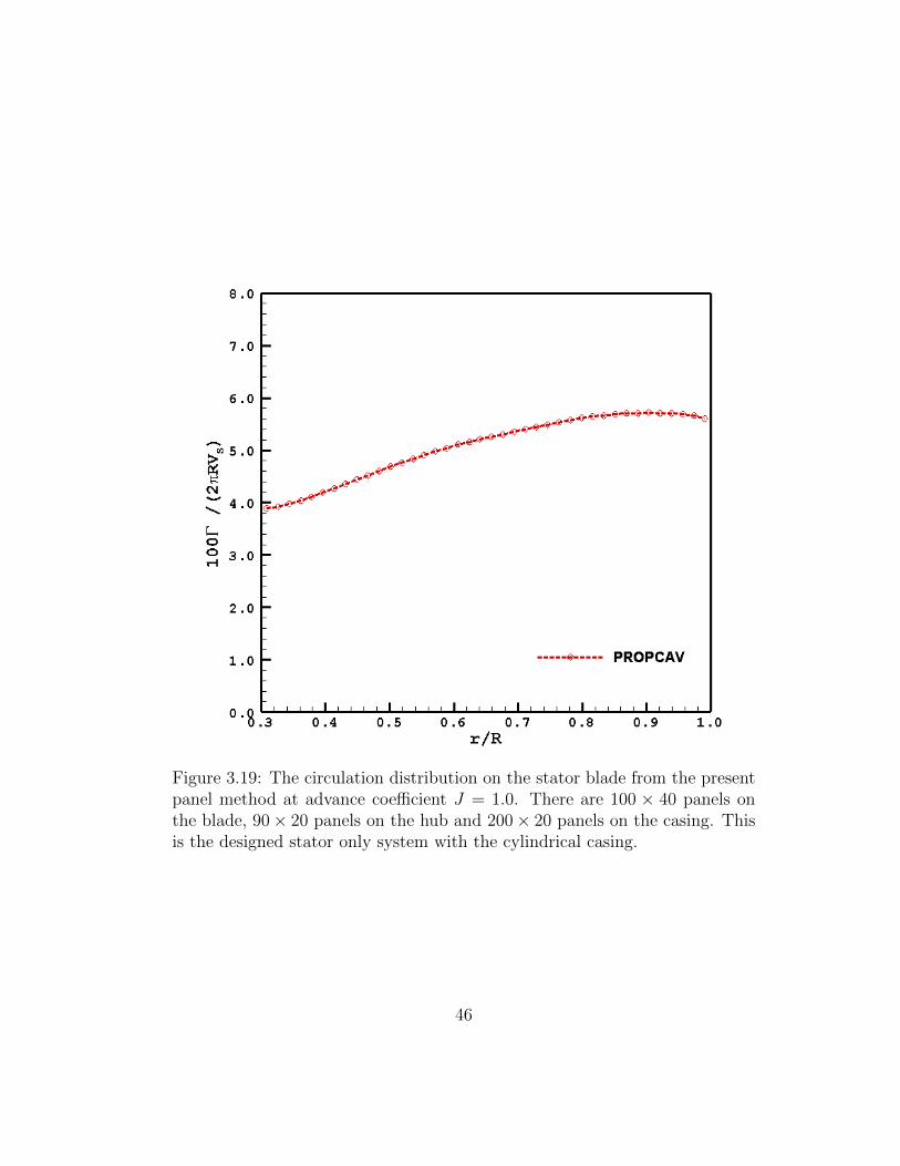
Figure 3.19: The circulation distribution on the stator blade from the presentpanel method at advance coefficient J = 1.0. There are 100 × 40 panels onthe blade, 90× 20 panels on the hub and 200× 20 panels on the casing. Thisis the designed stator only system with the cylindrical casing.
46

3.4 Rotor-stator interaction
The present panel method is able to analyze the rotor only problem and the
stator only problem successfully. This section presents the analysis of the
interaction between the rotor and the stator in the ONR-AXWJ2 water-jet
propulsion system using the induced velocity method.
The paneled geometry of the ONR-AXWJ2 water-jet system analysed with
the present numerical method is shown in Figure 3.20. The present method
takes about 120 minutes for 4 iterations between the rotor and stator by
utilizing one CPU. There are 120× 20 panels on the rotor and stator blades,
90× 20 panels on the hub and 160× 20 panels on the casing. The first
number in the legend 120× 20 denotes the number of panels in the
chord-wise or axial direction and the second number denotes the number of
elements in the span-wise direction on the blade or the circumferential
direction between two blades. There is no gap between the casing and the
blade in the simulation performed using the panel method.
A 3-D rotor-stator periodic mesh consisting of 4.2 million cells as shown in
Figure 3.21 is used to perform the RANS viscous simulation. The SIMPLEC
scheme is used for the pressure-velocity coupling in the simulation. There is
a gap of 0.33% between the casing and the rotor blade in the periodic mesh.
The realizable k − ε model with standard wall functions is used for the
viscous simulation. The mixing plane model is utilized for the rotor-stator
interaction. The stationary wall boundary condition is used on the stator
blade and the moving wall boundary condition on the hub, the rotor blade
47

and the casing. The y+ varies from 80 to 400 on the hub and from 100 to 250
on the casing. There are 10 layers in the tip gap region of the mesh. The
simulations take about 33 hours by using 32 CPUs to complete 20,000
iterations on a cluster with 2.43 GHZ quad-core 64-bit Intel Xeon processors
and 16 GB of RAM. The differences between the blade geometry used in
FLUENT and the present panel method are shown in 3.22.
The interactions between the rotor and the stator are performed in an
iterative manner until the forces on the rotor and stator converge. Figures
3.23 to 3.24 show the convergence details of the thrust and torque coefficients
on the rotor and stator respectively at advance coefficient J=1.19. The
interactions between the rotor and the stator converge after two iterations.
Figures 3.25 to 3.26 present the circulation distributions on the rotor and
stator blades respectively at different iterations. The zeroth iteration in
Figures 3.25 and 3.26 represent the rotor alone and stator alone results
respectively. It is observed that the effect of the stator on the rotor loading is
small whereas the effect of the rotor on the stator loading is considerable.
The Cp(mean) curves presented in Figures 3.27 and 3.28 are obtained by
circumferentially averaging pressures over all the strips on the casing surface
from the 3-D FLUENT simulation and those from the present panel method.
Figures 3.27 and 3.28 shows that the pressure rise on the casing surface from
the present panel method and the viscous FLUENT simulation are in good
agreement.
48
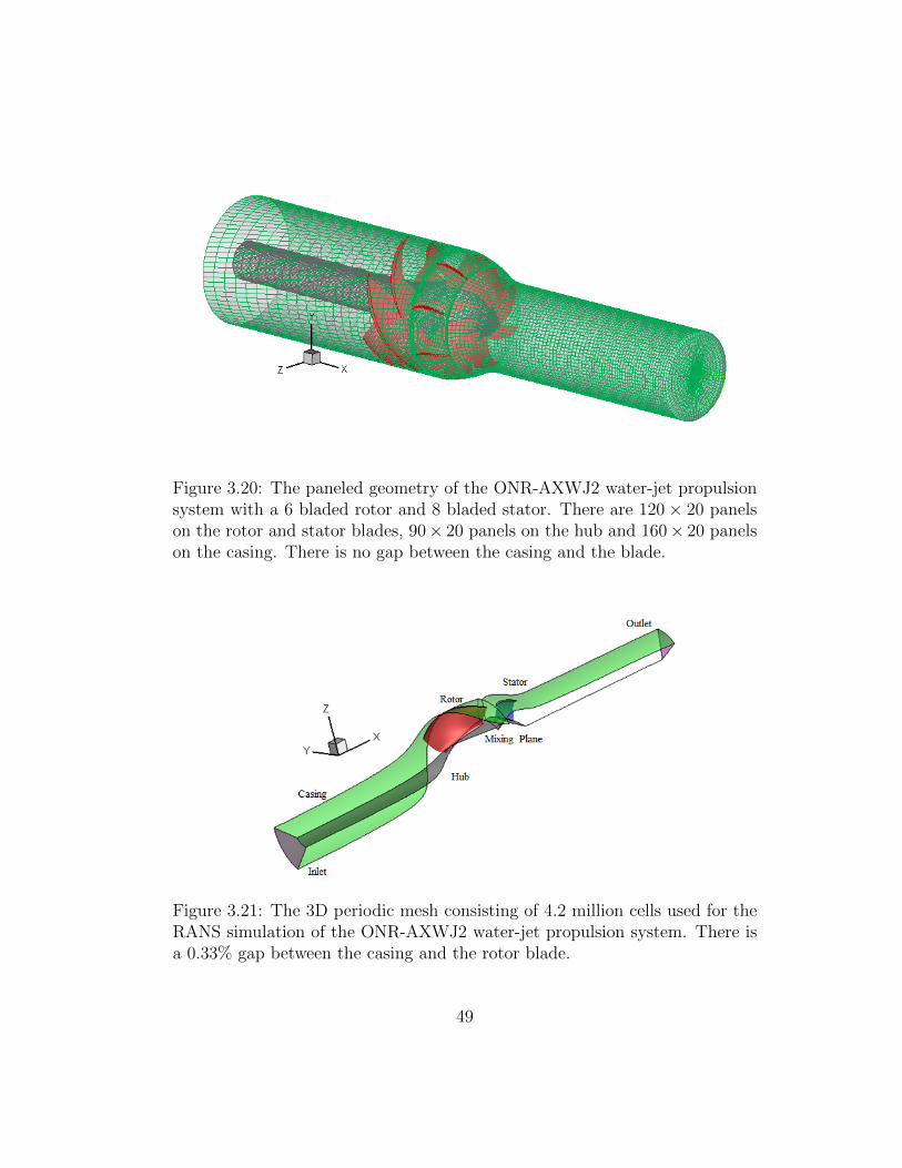
Figure 3.20: The paneled geometry of the ONR-AXWJ2 water-jet propulsionsystem with a 6 bladed rotor and 8 bladed stator. There are 120× 20 panelson the rotor and stator blades, 90× 20 panels on the hub and 160× 20 panelson the casing. There is no gap between the casing and the blade.
Figure 3.21: The 3D periodic mesh consisting of 4.2 million cells used for theRANS simulation of the ONR-AXWJ2 water-jet propulsion system. There isa 0.33% gap between the casing and the rotor blade.
49

Figure 3.22: Comparison of the ONR-AXWJ2 rotor blade geometry used inthe present panel method and FLUENT. The trailing edge of the rotor bladeused in FLUENT is blunt and the trailing edge of the blade used in the presentmethod is sharp with zero thickness (from Chang, 2012).
50

Figure 3.23: The thrust KT and torque KQ coefficients on the rotor bladefrom the present panel method at different iterations at an advance coefficientJ = 1.19. There are 120 × 20 panels on the blade, 90 × 20 panels on thehub and 160 × 20 panels on the casing. This is the ONR-AXWJ2 water-jetpropulsion system.
51
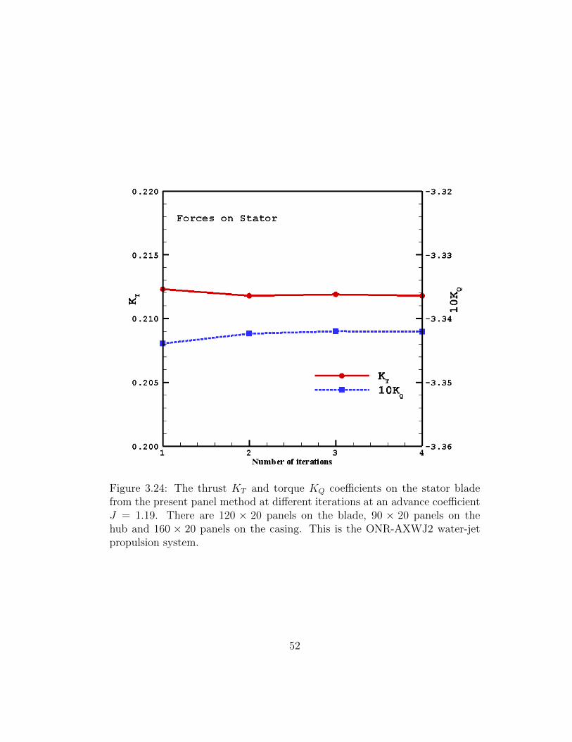
Figure 3.24: The thrust KT and torque KQ coefficients on the stator bladefrom the present panel method at different iterations at an advance coefficientJ = 1.19. There are 120 × 20 panels on the blade, 90 × 20 panels on thehub and 160 × 20 panels on the casing. This is the ONR-AXWJ2 water-jetpropulsion system.
52

Figure 3.25: The circulation distributions on the rotor blade from the presentpanel method at different iterations at an advance coefficient J = 1.19. Thereare 120×20 panels on the rotor blade, 90×20 panels on the hub and 160×20panels on the casing. This is the ONR-AXWJ2 water-jet propulsion system.
53

Figure 3.26: The circulation distributions on the stator blade from the presentpanel method at different iterations at an advance coefficient J = 1.19. Thereare 120×20 panels on the stator blade, 90×20 panels on the hub and 160×20panels on the casing. This is the ONR-AXWJ2 water-jet propulsion system.
54

Figure 3.27: Comparison of circumferentially averaged pressure distributionson the casing surface from the present panel method and FLUENT viscousrun at design advance coefficient J = 1.19. There are 120× 20 panels on theblade, 90× 20 panels on the hub and 160× 20 panels on the casing. The 3Dperiodic mesh has 4.2 million cells. There is a 0.33% gap between the casingand the rotor blade. This is the ONR-AXWJ2 water-jet propulsion system.
55

Figure 3.28: Comparison of circumferentially averaged pressure distributionson the casing surface from the present panel method and FLUENT viscousrun at advance coefficient J = 1.30. There are 120 × 20 panels on the blade,90× 20 panels on the hub and 160× 20 panels on the casing. The 3D periodicmesh has 4.2 million cells. There is a 0.33% gap between the casing and therotor blade. This is the ONR-AXWJ2 water-jet propulsion system.
56

Chapter 4
Numerical Analysis of Inducers
The present panel method is also extended to analyze rocket engine inducers.
An inducer is often used as a boost pump to raise the pressure for a
subsequent impeller. The formulation and solution of the Green’s integral
equation for the inducer problem is the same as the rotor only problem of a
water-jet system which has been presented in section 2.2.1. The present
study considers inducers subject to a uniform inflow and both the wetted
and the cavitating simulations are considered here.
4.1 Introduction
An inducer is an axial pump with blades that wrap in a helix around a
central core as shown in Figure 4.1. Inducers are widely used in rocket engine
turbo pumps to prevent cavitation in the pump main stages therefore
permitting higher turbo pump operating speeds and reduced pump inlet
pressure. Inducers can operate at low inlet pressures reducing the required
propellant tank pressure. Low tank pressures mean lighter propellant tanks.
At the same time, inducer supplies the main stage of the turbo pump with a
much higher pressure than is possible by tank pressurization, thus allowing
57

Figure 4.1: The geometrical configuration of a typical inducer used in rocketengines from Scheer et al. (1970).
the turbo pumps to operate at much higher speeds without cavitating.
4.2 Designed Inducer
This section presents the analysis of an inducer designed in-house by us,
labeled the Ocean Engineering Group (OEG) inducer, to validate the
numerical method. The inducer blade geometry is characterized by a low
pitch to diameter ratio of 0.5. The blades wrap in a helix around a hub as
shown in Figure 4.2. There are three blades in the inducer system. The
design advance coefficient J = 0.2652 for the fully wetted condition. There is
zero gap between the casing and the inducer blade in the panel method
simulation.
58

The panel method takes 12 minutes on a single CPU for a fully-wetted
analysis by using 120× 20 panels on the blade, 90× 20 panels on the hub
and 200× 20 panels on the casing. The first number in the legend 120× 20
denotes the number of panels in the chord-wise or axial direction and the
second number denotes the number of elements in the span-wise direction on
the blade or the circumferential direction between two blades.
The pressure distributions on the inducer blade sections from the present
panel method are compared with those from the RANS solver FLUENT. A
3-D periodic mesh consisting of 3.6 million cells as shown in Figure 4.3 is
used to perform the RANS simulation. The SIMPLEC scheme is used for the
pressure-velocity coupling in the simulation. The k − ω SST model is used
for the viscous simulation. The moving wall boundary condition is used on
the casing and the hub. The y+ varies from 40 to 380 on the hub and from
50 to 200 on the casing. The simulations take about 12 hours by using 16
CPUs to complete 20,000 iterations on a cluster with 2.43 GHZ quad-core
64-bit Intel Xeon processors and 16 GB of RAM.
Figures 4.5 to 4.7 show the pressure distributions on the inducer blade from
the present panel method and FLUENT viscous runs at different radii. The
results from the panel method are in very good agreement with the RANS
viscous calculations. The circulation distribution on the inducer blade from
the present panel method is given in 4.4.
59
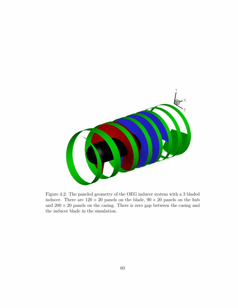
Figure 4.2: The paneled geometry of the OEG inducer system with a 3 bladedinducer. There are 120 × 20 panels on the blade, 90 × 20 panels on the huband 200× 20 panels on the casing. There is zero gap between the casing andthe inducer blade in the simulation.
60
Inflow
Rotor
Outlet
Hub
Figure 4.3: The 3D periodic mesh consisting of 3.6 million cells used for theRANS simulation. There is zero gap between the casing and the OEG inducerblade in the simulation.
61
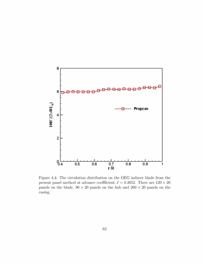
Figure 4.4: The circulation distribution on the OEG inducer blade from thepresent panel method at advance coeffficient J = 0.2652. There are 120× 20panels on the blade, 90 × 20 panels on the hub and 200 × 20 panels on thecasing.
62

Figure 4.5: Comparison of pressure distributions on the OEG inducer bladefrom the present panel method and FLUENT viscous run at advance coefficientJ = 0.2652 and radius of 0.43. There are 120×20 panels on the blade, 90×20panels on the hub and 160 × 20 panels on the casing. The 3D periodic meshhas 2.3 million cells.
63

Figure 4.6: Comparison of pressure distributions on the OEG inducer bladefrom the present panel method and FLUENT viscous run at advance coefficientJ = 0.2652 and radius of 0.70. There are 120×20 panels on the blade, 90×20panels on the hub and 200 × 20 panels on the casing. The 3D periodic meshhas 2.3 million cells.
64

Figure 4.7: Comparison of pressure distributions on the OEG inducer bladefrom the present panel method and FLUENT viscous run at advance coefficientJ = 0.2652 and radius of 0.97. There are 120×20 panels on the blade, 90×20panels on the hub and 200 × 20 panels on the casing. The 3D periodic meshhas 2.3 million cells.
65

Figure 4.8: The fabricated inducer from Scheer et al. (1970). The operatingconditions are at flow coefficient of 0.0084 which corresponds to an advancecoefficient J = 0.2652, 100% speed and a net positive suction head (NPSH) of32.3 m.
4.3 Industry Inducer
This inducer representative of typical rocket engine inducers was designed,
fabricated and tested to provide measurements of blade surface pressures and
stresses by Scheer et al. (1970) as shown in Figure 4.8. The operating
conditions are at flow coefficient of 0.0084 which corresponds to an advance
coefficient J = 0.2652, 100% speed and a net positive suction head (NPSH)
of 32.3 m.
The paneled geometry of the industry inducer system analyzed with the
66

present panel method is shown in Figure 4.9. The present method takes 12
minutes on a single CPU for a fully-wetted analysis by using 120× 20 panels
on the blade, 90× 20 panels on the hub and 200× 20 panels on the casing.
There is no gap between the casing and the blade in the simulation performed
using the panel method. The real size of the gap is 0.60% of the blade radius
but the gap is chosen to be sealed in the present approach since the tip gap
effect is not significant to the overall performance. The steady fully wetted
performance of the inducer subject to a uniform inflow is studied here.
The industry blade geometry provided to us is essentially constant thickness,
which suddenly tapers off at the leading and trailing edges as shown in
Figure 4.10. This introduces camber which can affect the pressure
distributions. Hence to ensure that there is no camber, we have modified the
industry blade sections. The new blade is created using the smooth lower
curve shown in Figure 4.10 as the centerline. The new blade section given in
Figure 4.11, has no camber and constant thickness everywhere except at the
leading and trailing edges where they are closed with elliptic ends.
The pressure distributions obtained from the present panel method are
compared with the experimental and RANS results at the tip radius
r/R = 0.94 and mean radius r/R = 0.68.The experimental results are
obtained from the report prepared by Scheer et al. (1970). The pressure is
expressed in terms of the static head coefficient defined as
ψs =g(p− pTo)
ρU2T
(4.1)
67
where p is the local static pressure, pTo is the inlet total pressure and UT is
the rotor tip speed.
The predicted circulation from the present panel method is positive and
nearly constant as shown in Figure 4.12. Figures 4.13 and 4.14 show the
pressure distributions on the inducer blade from the present panel method
and experiments at the mean radius and the tip radius respectively. The
results from the panel method are in reasonable agreement with the
experimental results.
Figure 4.9: The paneled geometry of the industry inducer system with a 3bladed blade. There are 120 × 20 panels on the blade, 90 × 20 panels on thehub and 200× 20 panels on the casing. There is zero gap between the casingand the inducer blade.
68

Figure 4.10: The original industry inducer blade geometry is essentially con-stant thickness which suddenly tapers off at the leading and trailing edges.
Figure 4.11: The new blade section of the industry inducer with no camber andconstant thickness everywhere except at the leading and trailing edge wherethey are closed with elliptic ends. Hence it is a constant thickness blade for97 % of the chord length.
69

Figure 4.12: The circulation distribution on the industry inducer blade fromthe present panel method at advance coefficient J = 0.2652.There are 120×20panels on the blade, 90 × 20 panels on the hub and 200 × 20 panels on thecasing.
70

Figure 4.13: Comparison of pressure distributions on the industry inducerblade from the present panel method and experimental results at advancecoeffficient J = 0.2652 and mean radius of 0.68. There are 120× 20 panels onthe blade, 90 × 20 panels on the hub and 200 × 20 panels on the casing.Theexperimental results are obtained from Scheer et al. (1970).
71

Figure 4.14: Comparison of pressure distributions on the industry inducerblade from the present panel method and experimental results at advancecoefficient J = 0.2652 and tip radius of 0.94. There are 120 × 20 panels onthe blade, 90 × 20 panels on the hub and 200 × 20 panels on the casing.Theexperimental results are obtained from Scheer et al. (1970).
72

4.4 Cavitating runs
Cavitating simulations are also performed for the industry inducer at a
cavitation number σ = 2.8977 and advance coefficient J = 0.2652. The
cavitation number is defined as
σ =p− pv0.5ρU2
(4.2)
where p is the local static pressure, pv is the vapor pressure and U is the
inflow speed.
The present method takes 16 minutes on a single CPU for a cavitating
analysis by using 120× 20 panels on the blade, 90× 20 panels on the hub
and 200× 20 panels on the casing. The circulation from the cavitating and
fully wetted simulations are shown in Figure 4.15. Figures 4.16 and 4.17
show the pressure distributions on the inducer blade from the cavitating and
fully wetted analysis at the mean radius and the tip radius respectively. The
cavity shapes on the inducer blade from the cavitating simulation are given
in Figure 4.18. The cavities are only present near the leading edge on the
suction side of the inducer blade in the cavitating simulation.
73

Figure 4.15: The predicted circulation distribution on the industry inducerblade from the cavitating and fully wetted simulations using the present panelmethod at an advance coeffficient J = 0.2652 and σ = 2.8977 .There are120× 20 panels on the blade, 90× 20 panels on the hub and 200× 20 panelson the casing.
74
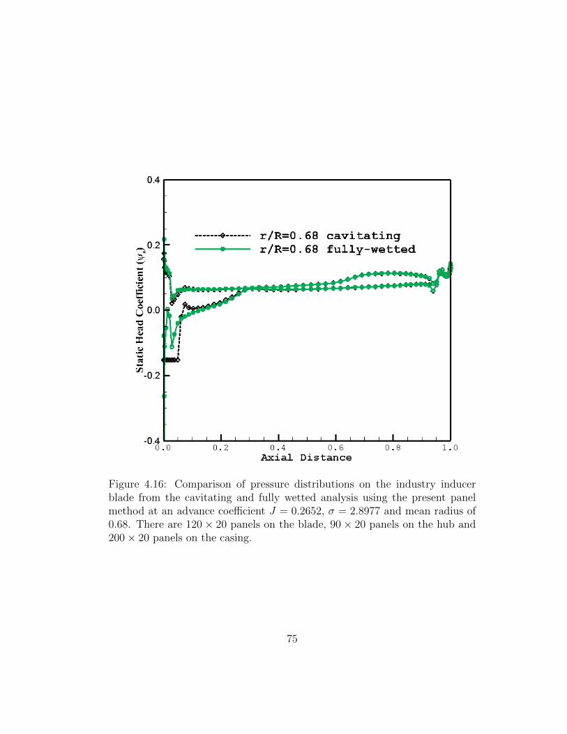
Figure 4.16: Comparison of pressure distributions on the industry inducerblade from the cavitating and fully wetted analysis using the present panelmethod at an advance coefficient J = 0.2652, σ = 2.8977 and mean radius of0.68. There are 120× 20 panels on the blade, 90× 20 panels on the hub and200× 20 panels on the casing.
75
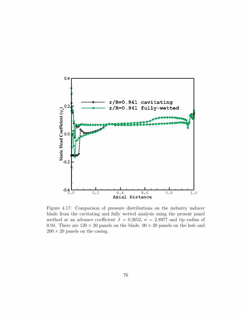
Figure 4.17: Comparison of pressure distributions on the industry inducerblade from the cavitating and fully wetted analysis using the present panelmethod at an advance coefficient J = 0.2652, σ = 2.8977 and tip radius of0.94. There are 120× 20 panels on the blade, 90× 20 panels on the hub and200× 20 panels on the casing.
76
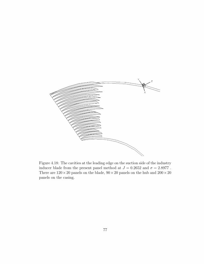
Figure 4.18: The cavities at the leading edge on the suction side of the industryinducer blade from the present panel method at J = 0.2652 and σ = 2.8977 .There are 120×20 panels on the blade, 90×20 panels on the hub and 200×20panels on the casing.
77

Chapter 5
Conclusions and future work
This chapter presents the conclusions derived from my research and outlines
the direction of the future work.
5.1 Conclusions
A numerical panel method based on inviscid irrotational flow theory and
utilizing hyperboloid panels has been developed and successfully applied for
the simulation of steady fully wetted flows inside water-jet pumps and rocket
engine inducers.
The source and dipole influence coefficients of non-planar hyperboloid panels
are accurately computed using Gauss quadrature. The numerical scheme is
validated by evaluating the influence coefficients for a non-planar
quadrilateral as well as the simplified case of a water-jet casing problem.
The numerical panel method is improved significantly to predict the
hydrodynamic performance parameters of a water-jet propulsion system. The
present method solves the boundary value problem subject to a uniform
inflow directly by simulating the blade, casing/shroud and hub geometries as
discretized panels. The Green’s integral equation and the influence
78
coefficients for the water-jet/inducer problem are defined and solved by
spreading constant strength dipoles and sources on the blade, hub and casing
surfaces and constant strength dipoles on the shed wake sheets behind the
rotor/ stator blades. The circulation and pressure distributions for the rotor
alone problem and the stator alone problems are found to be in good
agreement with RANS calculations obtained using FLUENT. The pressure
rise on the casing is successfully estimated for the rotor only case using the
numerical panel method.
The rotor- stator interaction is accomplished using an iterative procedure
which considers the effect of circumferentially averaged induced velocities
between the rotor and the stator. The iterations for the rotor-stator problem
converge quickly. The influence of the stator on the rotor loading is observed
to be small. The pressure rise on the casing for the ONR-AXWJ2 water-jet
propulsion system is obtained using the numerical panel method and is in
good agreement with the FLUENT results. The panel method also requires
significantly less computational time compared to RANS solvers.
The numerical panel method is also successfully extended to analyze rocket
engine inducers. The formulation and solution of the Green’s integral
equation for the inducer problem is found to be very similar to the rotor only
problem of a water-jet system. The circulation and pressure distributions on
the inducer blade sections are found to be in good agreement with
experimental results and RANS calculations obtained using FLUENT. The
panel method is also utilized to predict the cavity shapes on the inducer
79

blade.
5.2 Future work
There are multiple avenues for advancing and improving the present
numerical method. A few of them are listed in this section.
In reality, the rotor and stator blade geometries have blunt trailing edges.
The present panel method can be modified to handle blunt trailing edges by
adopting the approach given by Purohit (2013) which obtains a non-lifting
sharp extension for finite trailing edges and includes the three dimensional
geometry effects when coupling with XFOIL.
The effects of viscosity on the rotor and stator blades can be included by
coupling the present panel method with XFOIL to solve the water-jet
system. The present panel method needs to be extensively analyzed for
cavitating water-jet systems and used to predict the thrust and torque
breakdowns as given in Chang (2012).
The present panel method can also be extended to replicate the unsteady
interaction between the rotor and the stator using the method developed by
He (2010) and Tian (2013). The water-jet propulsion system also needs to be
analyzed for unsteady inflows.
80

Appendix
81

Appendix 1
Formulation of 2D and 3D Influence
Coefficients
The definitions of the dipole and the source influence coefficients for the 2D
and 3D panels are listed here.
1.1 2D Influence Coefficients
• Dipole
Aij =1
2π
∫S
∂ ln r
∂nds (1.1)
• Source
Bij =1
2π
∫S
ln rds (1.2)
where ds is the elemental length.
1.2 3D Influence Coefficients
• Dipole
Aij =1
4π
∫S
∂(1/r)
∂nds (1.3)
• Source
Bij =1
4π
∫S
1
rds (1.4)
82

where ds is the elemental surface area.
83

Bibliography
[1] S. Brewton, S. Gowing, and J. Gorski. Performance predictions of a
waterjet rotor and rotor/stator combination using rans calculations. In
Proc. 26th Symposium on Naval Hydrodynamics, Rome, Italy, 2006.
[2] S.H. Chang. Numerical Simulation of Steady and Unsteady Cavitating
Flows inside Water-jets. PhD thesis, Department of Civil Engineering,
UT Austin, August 2012.
[3] H. H. Chun, W. G. Park, and J. G. Jun. Experimental and cfd analysis
for rotor-stator interaction of a water-jet pump. In Proc. 24th
Symposium on Naval Hydrodynamics, Fukuoka, Japan, 2002.
[4] M. Drela. XFOIL: An analysis and design system for low Reynolds
number airfoils. In Lecture Notes in Engineering (Volume 54, Low
Reynolds Number Aerodynamics), New York, 1989. Springer-Verlag.
[5] L. He. Numerical Simulation of Unsteady Rotor/Stator Interaction and
Application to Propeller/Rudder Combination. PhD thesis, Department
of Civil Engineering, UT Austin, August 2010.
[6] J. E. Kerwin. Final report and recommendations to the 25th ittc,
specialist committee on cavitation. In Proc. 25th International Towing
Tank Conference, volume II, pages 473–533.
84

[7] J. E. Kerwin. Hydrodynamic issues in water-jet design and analysis. In
Proc. 26th Symposium on Naval Hydrodynamics, Rome, Italy, 2006.
[8] J. E. Kerwin, T. E. Taylor, and G. P. Black, S. D.and McHugh. A
coupled lifting-surface analysis technique for marine propulsors in steady
flow. In Proc. Society of Naval Architects and Marine Engineers
Propellers and Shafting Symposium, Virginia Beach, VA, United States,
1997.
[9] M.C. Kim, J.G. Jun, W.G. Park, and H.H. Chun. Flow analysis on the
inside of duct for the waterjet system of tracked vehicle with
consideration of interaction of rotor and stator. In Proceedings of Spring
Meeting of the Society of Naval Architect of Korea, Korea, 2002.
[10] S. A. Kinnas, S.H. Chang, and Y.H. Yu. Prediction of wetted and
cavitating performance of water-jet. In Proc. 28th Symposium on Naval
Hydrodynamics, Pasadena, CA, 2010.
[11] S. A. Kinnas and N. E. Fine. A numerical nonlinear-analysis of the flow
around 2-dimensional and 3-dimensional partially cavitating hydrofoils.
J. Fluid Mech, pages 151–181, 1994.
[12] S. A. Kinnas and C.-Y. Hsin. A boundary element method for the
analysis of the unsteady flow around extreme propeller geometries.
AIAA Journal, pages 688–696, 1992.
85

[13] S. A. Kinnas, H. S. Lee, T. J. Michael, and H. Sun. Prediction of
cavitating water-jet propulsor performance using a boundary element
method. In Proc. 9th Int. Conf. on Numerical Ship Hydrodynamics,,
Ann Arbor, Michigan, 2007.
[14] S. A. Kinnas, H. S. Lee, H. Sun, and L. He. Performance prediction of
single or multi-component propulsors using coupled viscous/inviscid
methods,. In Proc. 10th Int. Symposium on the Practical Design of
Ships and other Floating Structures, Houston, TX, 2007.
[15] S. A. Kinnas, Alokraj Valsaraj, and S.H. Chang. A panel method for
the hydrodynamic performance prediction of a water-jet and an inducer.
In Propeller and Shafting Symposium 2012, Norfolk,Virginia, 2012.
[16] J. W. Lindau, W. L. Moody, M. P. Kinzel, J. J. Dreyer, R. F. Kunz, and
E. G. Paterson. Computation of cavitating flow through marine
propulsors. In Int. Symposium on Marine Propulsors, Trondheim,
Norway, 2009.
[17] L. Morino and C.C. Kuo. Subsonic potential aerodynamics for complex
configuration: a general theory. AIAA Journal, pages 191–197, 1974.
[18] L. Morino, Chen Lee, and Emil O.Suciu. Steady and oscillatory
subsonic and supersonic aerodynamics around complex configurations.
AIAA Journal, 1975.
86

[19] J.N.. Newman. Distributions of sources and normal dipoles over a
quadrilateral panel. Journal of Engineering Mathematics, pages
113–126, 1986.
[20] Jai Purohit. Numerical simulation of ducted propellers. Master’s thesis,
Department of Civil Engineering, UT Austin, August 2013.
[21] D.D. Scheer. Study of inducer load and stresses. Technical report,
NASA, December 1970.
[22] H. Sun and S. A. Kinnas. Simulation of sheet cavitation on propulsor
blades using a viscous/inviscid interactive method. In Proc. 28th
Symposium on Naval Hydrodynamics, Wageningen, Netherlands, 2006.
[23] T. E. Taylor and J. O. Kerwin, J. E.and Scherer. Water-jet pump
design and analysis using a coupled lifting-surface and rans procedure.
In Proc. Int. Conf. on Water-jet Propulsion, The Royal Institution of
Naval Architects,, London, UK, 1998.
[24] Ye Tian and S. A. Kinnas. A numerical method for the analysis of
unsteady cavitating rotor and stator interaction. In Third International
Symposium on Marine Propulsors, Launceston, Tasmania, Australia,
2013.
87

Vita
Alokraj Valsaraj was born in Kannur, Kerala, India along with his twin
brother Amithraj Valsaraj on 30th November 1988, the son of R.Valsaraj
and P.Lathika. He recieved the Bachelor of Technology in Naval Architecture
and Ocean Engineering from Indian Institute of Technology Madras in July
2011. In August 2011, he started his graduate studies as a member of the
Ocean Engineering Group at The University of Texas at Austin.
Permanent address: 15000 Park Row, Apt 228Houston, Texas 77084
This thesis was typeset with LATEX† by the author.
†LATEX is a document preparation system developed by Leslie Lamport as a specialversion of Donald Knuth’s TEX Program.
88