Ocean circulation and air-sea interaction - ECMWF · Beneﬁts of a CMS. Ocean circulation and air-sea interaction Peter Janssen, Magdalena Balmaseda, Jean Bidlot, Øyvind Breivik,

. Benefits of a CMS .

Ocean circulation and air-sea interaction

Peter Janssen, Magdalena Balmaseda, Jean Bidlot, Øyvind Breivik, Sarah Keeley,

Martin Leutbecher, Linus Magnusson, Kristian Mogensen and Frederic Vitart

European Centre for Medium-Range Weather Forecasts

<[email protected]>

1 .


INTRODUCTION

In this talk I would like to discuss air-sea interaction in the context of a

coupled modelling system(CMS). We have developed a CMS which at the

moment consists of three components:

1. atmosphere (IFS)

2. ocean waves (WAM)

3. and the ocean/sea-ice (NEMO)

These three components have been brought together in a single executable.

2 .


Today, I discuss briefly the following items:

• Numerics of the coupling

As occasionally there is a strong coupling between the threecomponents of the

CMS there is a need to study the numerical scheme involved in such a coupling.

For example, if the coupling is strong are there possibilities of numerical

instability, do we need to couple in an implicit manner? Do weneed an

energy/momentum conserving interpolation scheme, etc...

So far I am not aware of a systematic study of this problem. I will give an

example of a serious problem we had in the early part of this Century, namely the

generation ofmini vortices by the coupling between wind and ocean waves,

and how this was fixed.

3 .


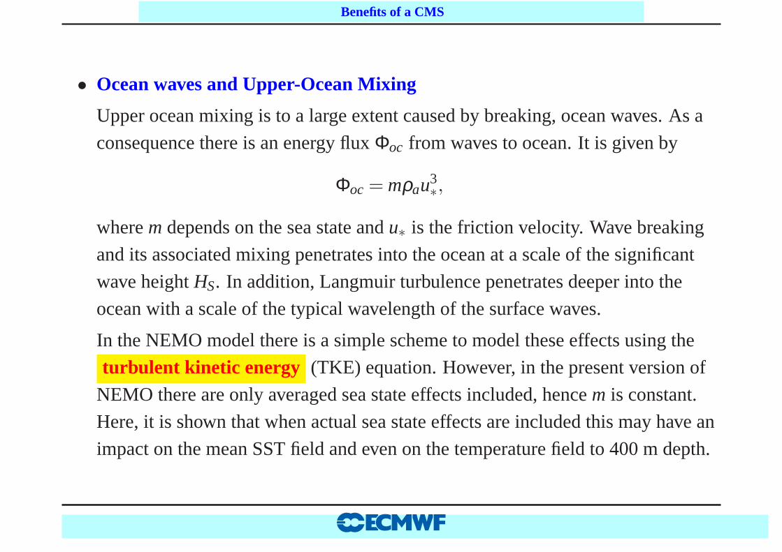
• Ocean waves and Upper-Ocean Mixing

Upper ocean mixing is to a large extent caused by breaking, ocean waves. As a

consequence there is an energy fluxΦoc from waves to ocean. It is given by

Φoc = mρau3∗,

wherem depends on the sea state andu∗ is the friction velocity. Wave breaking

and its associated mixing penetrates into the ocean at a scale of the significant

wave heightHS. In addition, Langmuir turbulence penetrates deeper into the

ocean with a scale of the typical wavelength of the surface waves.

In the NEMO model there is a simple scheme to model these effects using the

turbulent kinetic energy (TKE) equation. However, in the present version of

NEMO there are only averaged sea state effects included, hence m is constant.

Here, it is shown that when actual sea state effects are included this may have an

impact on the mean SST field and even on the temperature field to400 m depth.

4 .


• Coupling from Day 0

Presently, in the operational medium-range/monthly ensemble forecasting

system (ENS) the interaction between atmosphere and ocean is only switched on

at Day 10 in the forecast. In the autumn a new version of ENS/monthly will be

introduced in operations where the coupling starts from Day0. Also, sea state

effects on upper ocean mixing and dynamics will be switched on.

Coupling from Day 0 has beneficial impacts on hurricane forecasting, the MJO

and the statistical properties of ENS.

5 .


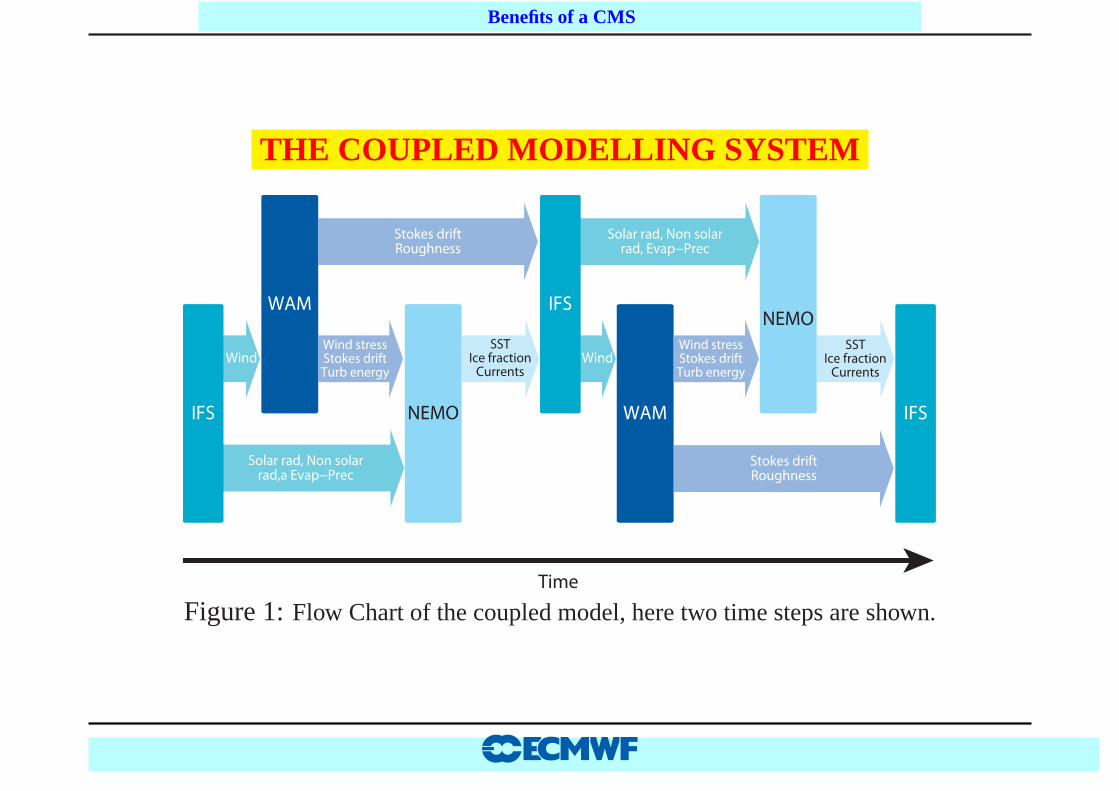
THE COUPLED MODELLING SYSTEM

Solar rad, Non solarrad, Evap−Prec

WAM

Wind Wind

Stokes driftRoughness

Stokes driftRoughness

WAM

Solar rad, Non solarrad,a Evap−Prec

IFS

NEMO IFS

SSTIce fraction

Currents

SSTIce fraction

Currents

NEMO

Time

Wind stressStokes driftTurb energy

Wind stressStokes driftTurb energy

IFS

Figure 1:Flow Chart of the coupled model, here two time steps are shown.

6 .


Numerics of the coupling

I will give two examples that occasionally there is a strong coupling between the

three components of the CMS. One example involves the deepening of a low during

IOP17 of FASTEX (atm=ocean-wave) another example involveshurricane Nadine

and the cooling of SST by the strong wind circulation.

7 .


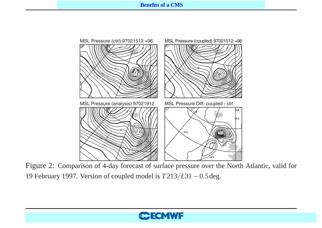
MSL Pressure (ctrl) 97021512 +96 MSL Pressure (coupled) 97021512 +96

MSL Pressure (analysis) 97021912 MSL Pressure Diff. coupled - ctrl

Figure 2:Comparison of 4-day forecast of surface pressure over the North Atlantic, valid for

19 February 1997. Version of coupled model isT213/L31−0.5deg.

8 .


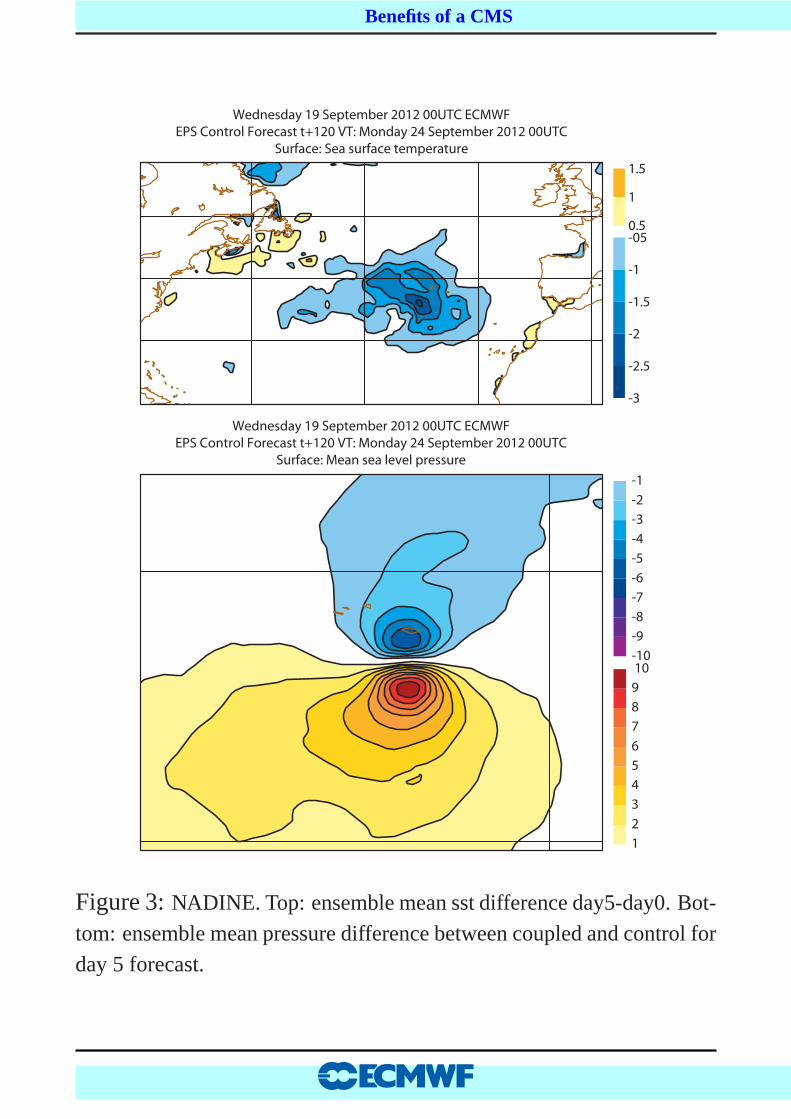
Wednesday 19 September 2012 00UTC ECMWFEPS Control Forecast t+120 VT: Monday 24 September 2012 00UTC

Surface: Sea surface temperature

-3

-2.5

-2

-1.5

-1

-050.5

1

1.5

Wednesday 19 September 2012 00UTC ECMWFEPS Control Forecast t+120 VT: Monday 24 September 2012 00UTC

Surface: Mean sea level pressure

1

2

3

4

5

6

7

8

9

10-10

-9

-8

-7

-6

-5

-4

-3

-2

-1

Figure 3:NADINE. Top: ensemble mean sst difference day5-day0. Bot-

tom: ensemble mean pressure difference between coupled andcontrol for

day 5 forecast.

9


Because of this occasional strong interaction between atmosphere and ocean waves

there is a need to study the numerical scheme involved in sucha coupling. For

example, if the coupling is strong are there possibilities of numerical instability, is

there a need to couple in an implicit manner, etc.

This might require a systematic study. I will give one example, namely the generation

of spurious mini-vortices caused by the coupling between wind and ocean waves.

10 .


Generation of spurious mini-vortices

1. Two-way interaction of wind and waves was introduced on June 29 1998. The

coupling time step was 4 wave model time steps, hence ample time for the wave

model to respond to rapidly varying winds, resulting in realistic values of the

roughness length.

2. With the introduction of theTL511 version of the IFS the coupling time step was

reduced to one wave model time step. From the start of the operational

introduction occasional small scale, compact features occurred in the surface

pressure field that propagated rapidly over the oceans. Called mini-vortices, or

evencannon balls.

11 .


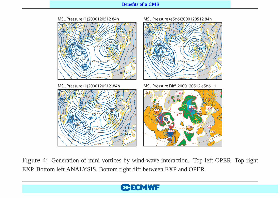
MSL Pressure (1)2000120512 84h MSL Pressure (e5q6)2000120512 84h

MSL Pressure (1)2000120512 84h MSL Pressure Di!. 2000120512 e5q6 - 1

Figure 4: Generation of mini vortices by wind-wave interaction. Top left OPER, Top right

EXP, Bottom left ANALYSIS, Bottom right diff between EXP andOPER.

12 .


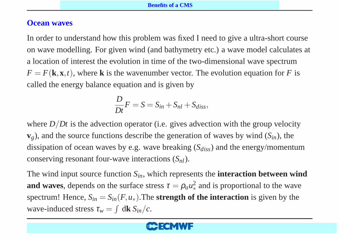
Ocean waves

In order to understand how this problem was fixed I need to givea ultra-short course

on wave modelling. For given wind (and bathymetry etc.) a wavemodel calculates at

a location of interest the evolution in time of the two-dimensional wave spectrum

F = F(k,x, t), wherek is the wavenumber vector. The evolution equation forF is

called the energy balance equation and is given by

DDt

F = S = Sin +Snl +Sdiss,

whereD/Dt is the advection operator (i.e. gives advection with the group velocity

vg), and the source functions describe the generation of wavesby wind (Sin), the

dissipation of ocean waves by e.g. wave breaking (Sdiss) and the energy/momentum

conserving resonant four-wave interactions (Snl).

The wind input source functionSin, which represents theinteraction between windand waves, depends on the surface stressτ = ρau2

∗and is proportional to the wave

spectrum! Hence,Sin = Sin(F,u∗).Thestrength of the interaction is given by the

wave-induced stressτw =∫

dk Sin/c.

13 .


In the 1980’s there was a considerable European effort to build a wave prediction

system based on solving the energy balance equation.

The integration in time was done with a (semi-) implicit scheme as follows.

1. Calculate dimensionless roughness or the Charnock parametergz0/u2∗

from

wave-induced stress att = tn and wind speed at new time leveltn+1. Calculate

friction velocity un+1∗

2. Spectral increments∆F are obtained from an implicit scheme:

∆F = ∆tSn(un+1∗

)

[

1−∆tδSn

δF(un+1

∗)

]

−1

Problem is that under rapidly varying winds (e.g. sudden dropin wind) the waves are

still steep given a far too large roughness. This results in considerably enhanced heat

fluxes that may generate a mini vortex.

Fix: Do the roughness calculation also after the spectral update Fn+1 = Fn +∆F .

14 .


0 6 120

0.05

0.1

0.15

0.2

0.25

Charnock parameter versus timeFront passes at 6 o’clock

OLD

NEW

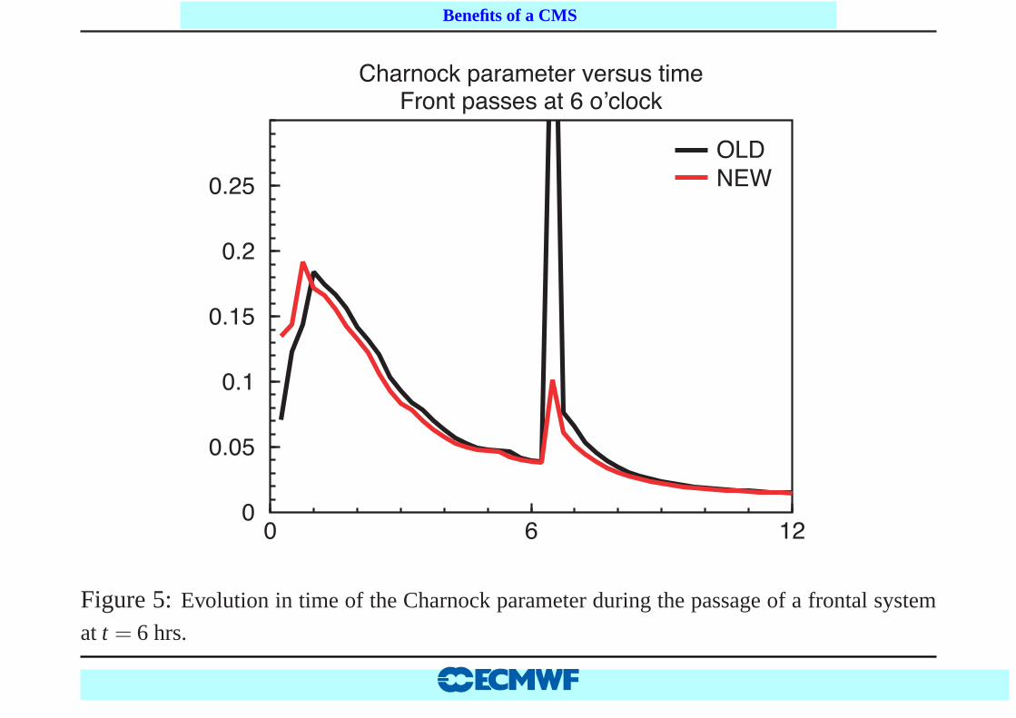
Figure 5:Evolution in time of the Charnock parameter during the passage of a frontal system

at t = 6 hrs.

15 .


MSL Pressure (1)2000120512 84h MSL Pressure (e5q6)2000120512 84h

MSL Pressure (1)2000120512 84h MSL Pressure Di!. 2000120512 e5q6 - 1

Figure 6: Generation of mini vortices by wind-wave interaction. Top left OPER, Top right

EXP, Bottom left ANALYSIS, Bottom right diff between EXP andOPER.

16 .


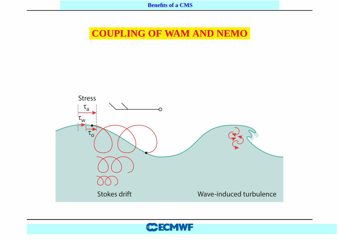
COUPLING OF WAM AND NEMO

τa

τw

τo

Stokes drift Wave-induced turbulence

Stress

17 .


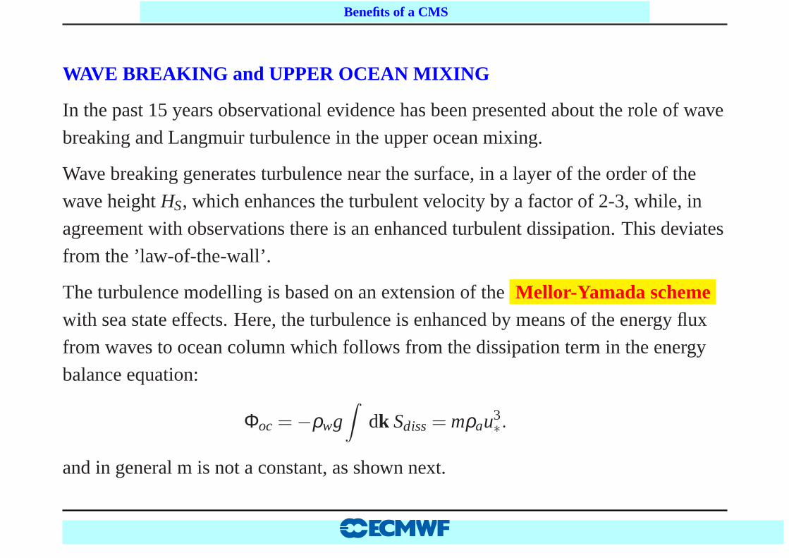
WAVE BREAKING and UPPER OCEAN MIXING

In the past 15 years observational evidence has been presented about the role of wave

breaking and Langmuir turbulence in the upper ocean mixing.

Wave breaking generates turbulence near the surface, in a layer of the order of the

wave heightHS, which enhances the turbulent velocity by a factor of 2-3, while, in

agreement with observations there is an enhanced turbulentdissipation. This deviates

from the ’law-of-the-wall’.

The turbulence modelling is based on an extension of theMellor-Yamada schemewith sea state effects. Here, the turbulence is enhanced by means of the energy flux

from waves to ocean column which follows from the dissipation term in the energy

balance equation:

Φoc =−ρwg∫

dk Sdiss = mρau3∗.

and in general m is not a constant, as shown next.

18 .


0°N

10°S

20°S

30°S

40°S

50°S

60°S

10°N

20°N

30°N

40°N

50°N

60°N

70°N

80°N

0°N

10°S

20°S

30°S

40°S

50°S

60°S

10°N

20°N

30°N

40°N

50°N

60°N

70°N

80°N

0°E20°W40°W60°W80°W100°W120°W140°W160°W180°W160°E140°E 20°E 40°E 60°E 80°E 100°E

0°E20°W40°W60°W80°W100°W120°W140°W160°W180°W160°E140°E 20°E 40°E 60°E 80°E 100°E

from 1 October 2010 to 30 September 2012Normalised mean of the energy flux into the ocean from ERA-Interim analysis

1.8 2 2.2 2.4 2.6 2.8 3 3.2 3.4 3.6 3.8 4 4.2 4.4 4.6

Figure 7:Mean of energy flux into the ocean, normalized with the mean ofρau3∗. Averaging

period is two years.

19 .


TKE EQUATION

If effects of advection are ignored, the turbulent kinetic energy (TKE) equationdescribes the rate of change of turbulent kinetic energye due to processes such asshear production (including the shear in the Stokes drift),damping by buoyancy,vertical transport of TKE, and turbulent dissipationε. It reads

∂e∂ t

=∂∂ z

(

νq∂e∂ z

)

+νmS2+νmS∂US

∂ z−νhN2

− ε ,

wheree = q2/2, with q the turbulent velocity,S = ∂U/∂ z andN2 = gρ−10 ∂ρ/∂ z,

with N the Brunt-Vaisala frequency. The eddy viscosities for momentum, heat, andTKE are denoted byνm, νh andνq. E.gνm = l(z)q(z)SM wherel(z) is the mixinglength andSM depends on stratification.

Wave-induced turbulence is introduced by the boundary condition:

ρwνq∂e∂ z

= Φoc,z = 0.

while effects of Langmuir turbulence are introduced by the term involving the shearin the Stokes-drift profile.

20 .


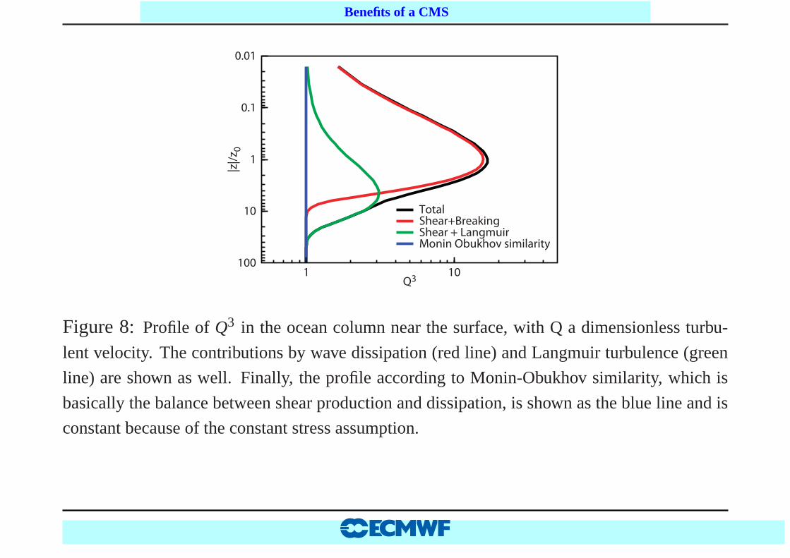
In the next Figure we show an approximate solution to the TKE equation which

illustrates that wave breaking enhances turbulence up to a depth of a few wave

heights, while Langmuir turbulence acts in the deeper partsof the ocean. For

comparison, results for Monin-Obukhov similarity (from balance of turbulent shear

production and turbulent dissipation) are shown as well.

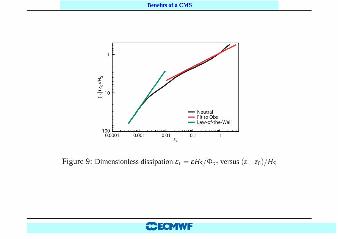
The following Figure shows a comparison between the profile of modelled dissipation

and a fit to observations of turbulence dissipation. The law-of-the wall follows from

ε = νmS2,

which for a constant stress, i.e.νmS = const, gives an inverse dependence on the

distance from the surface.

21 .


0.01

0.1

1 10Q3

1

10

100

|z|/

z 0

TotalShear+BreakingShear + LangmuirMonin Obukhov similarity

Figure 8: Profile of Q3 in the ocean column near the surface, with Q a dimensionless turbu-

lent velocity. The contributions by wave dissipation (red line) and Langmuir turbulence (green

line) are shown as well. Finally, the profile according to Monin-Obukhov similarity, which is

basically the balance between shear production and dissipation, is shown as the blue line and is

constant because of the constant stress assumption.

22 .


0.0001 0.001 0.01 0.1 1ε∗

1

10

100

(|z|

+z 0

)/H

S

NeutralFit to ObsLaw-of-the-Wall

Figure 9:Dimensionless dissipationε∗ = εHS/Φoc versus(z+ z0)/HS

23 .


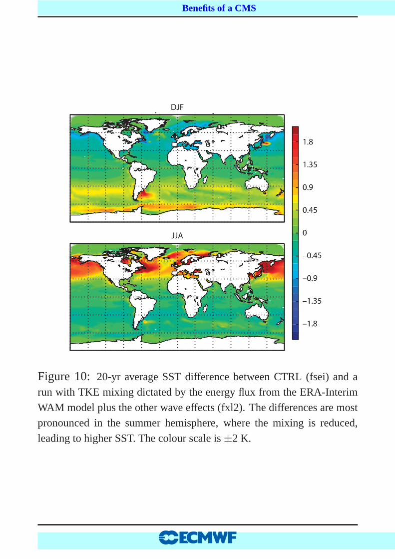
IMPACT ON MEAN SST FIELD

We introduced the sea state dependent upper ocean mixing in the NEMO model.

The ocean circulation equations are very similar to the hydrostatic equations for the

atmosphere, except, of course no clouds, but rather salinity.

A number of methods are used to advance these equations (discretized on an Arakawa

C grid) in time. The non-diffusive parts are treated by a leapfrog scheme, while for

the diffusive parts a forward/backward time differencing scheme is used. By

introducing a semi-implicit computation of the hydrostatic pressure gradient term the

stability range of the leap frog scheme can be extended by a factor of two.

Show results from standalone runs, forced by ERA-interim fluxes and seastate.

Averages are over a 20 year period. The control run is one where the dimensionless

energy flux is a constant, given bym = 3.5.

24 .


DJF

JJA

1.8

1.35

0.9

0.45

0

–0.45

–0.9

–1.35

–1.8

Figure 10: 20-yr average SST difference between CTRL (fsei) and a

run with TKE mixing dictated by the energy flux from the ERA-Interim

WAM model plus the other wave effects (fxl2). The differences are most

pronounced in the summer hemisphere, where the mixing is reduced,

leading to higher SST. The colour scale is±2 K.

25


SST STDE WAM

100E 150E 160W 110W 60W 10W

0

20N

40N

60N

80N

Lati

tud

e

0 0.2 0.4 0.6 0.8 1 1.2 1.4 1.6 1.8 2

SST STDE CTRL

(deg C): Min= 0.06, Max= 3.51, Int= 0.10

100E 150E 160W 110W 60W 10WLongitude

0

20N

40N

60N

80N

(deg C): Min= 0.07, Max= 2.76, Int= 0.10Longitude

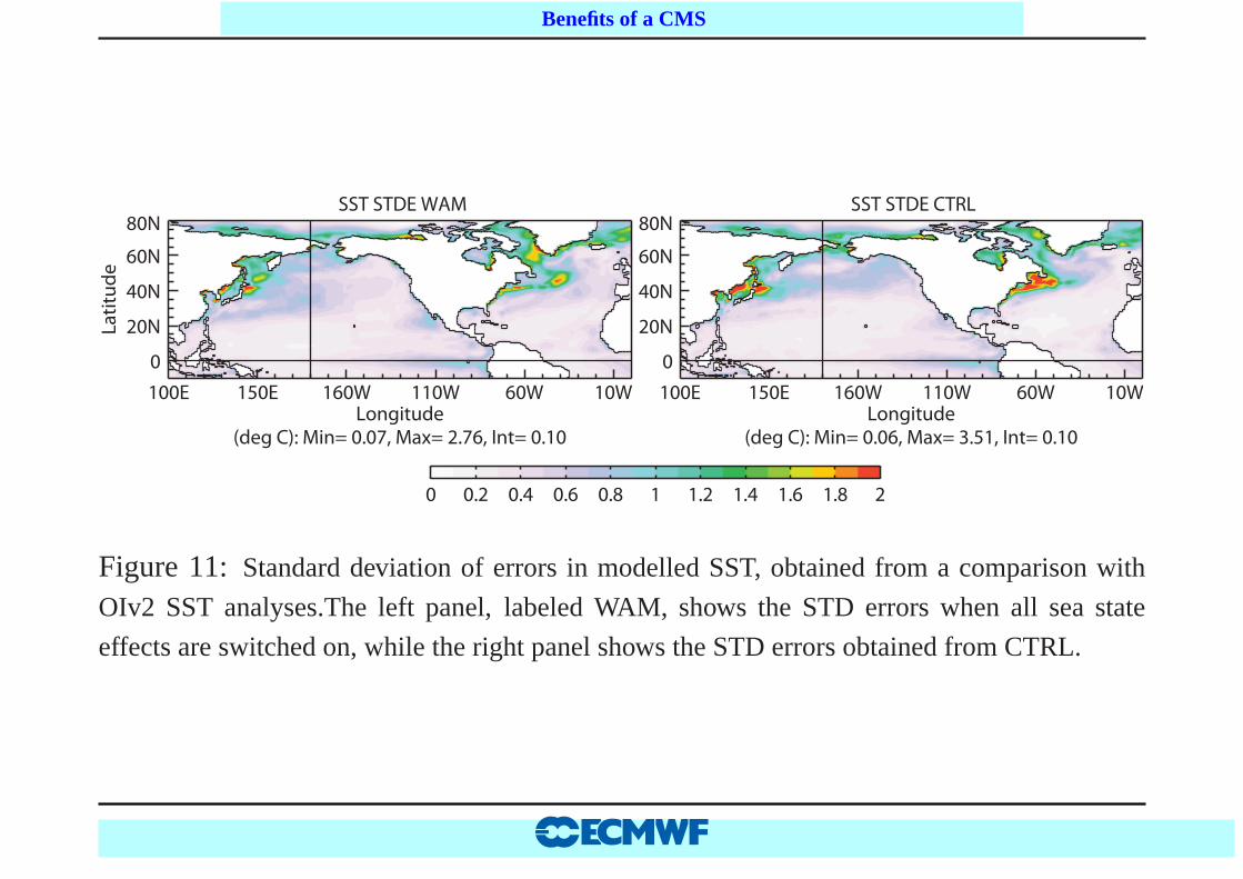
Figure 11: Standard deviation of errors in modelled SST, obtained froma comparison with

OIv2 SST analyses.The left panel, labeled WAM, shows the STDerrors when all sea state

effects are switched on, while the right panel shows the STD errors obtained from CTRL.

26 .


WAM-CTRL 170E-T

longitudes in [169.5, 170.5] - (3 points) (deg C): Min= -1.59, Max= 1.58, Int= 0.1

50S 0 50NLatitude

6000

4000

2000

500

400

300

200

100

0

De

pth

(m)

-1 -0.8 -0.6 -0.4 -0.2 0 0.2 0.4 0.6 0.8 1

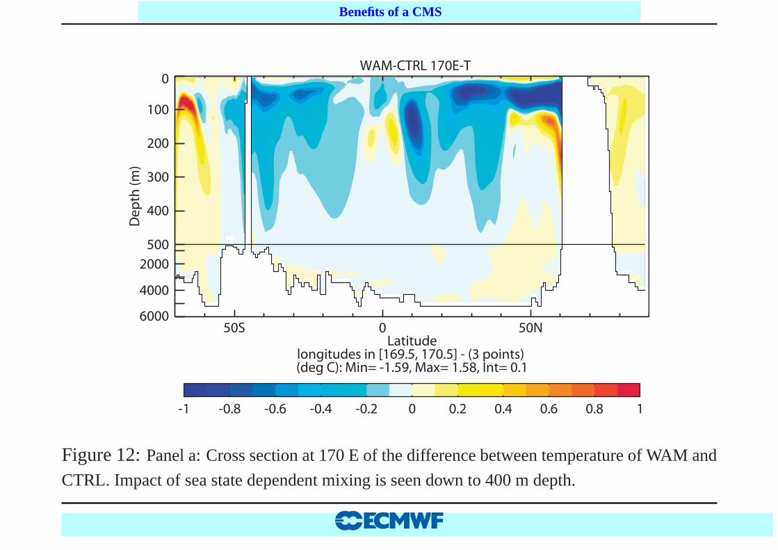
Figure 12:Panel a: Cross section at 170 E of the difference between temperature of WAM and

CTRL. Impact of sea state dependent mixing is seen down to 400m depth.

27 .


IMPACT ON COUPLED RUNS

Next, we study results from coupled seasonal forecast runs.Again, the control run is

one where the dimensionless energy flux is a constant, given by m = 3.5.

As the control gave substantial biases, and seasonal forecasting skill is very sensitive

to systematic errors we used an additional control run with areduced value ofm,

m = 0.56, which had very similar systematic errors as the experiment with seastate

effects included. Surprisingly, in certain areas this had anegative impact on forecasts

skill. At the moment, we are at a loss how to properly interpret the skill scores of the

seasonal forecasting system.

28 .


90°E

–7 –3 –2.5 –2 –1.5 –1 –0.5 0.5 1 1.5 2 2.5 3 6

60°S

30°S

0°

30°N

60°N

180°W

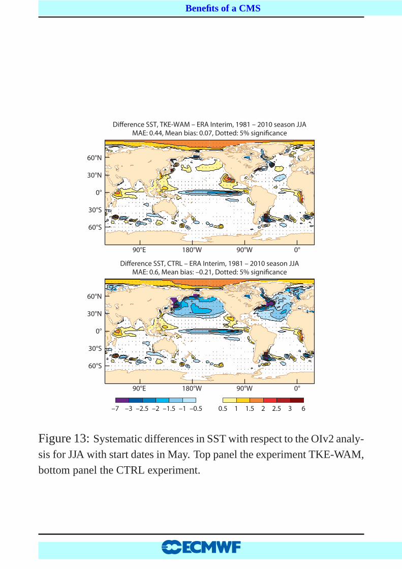
Di�erence SST, TKE-WAM – ERA Interim, 1981 – 2010 season JJA

MAE: 0.44, Mean bias: 0.07, Dotted: 5% signi�cance

Di�erence SST, CTRL – ERA Interim, 1981 – 2010 season JJA

MAE: 0.6, Mean bias: –0.21, Dotted: 5% signi�cance

90°W 0°

90°E

60°S

30°S

0°

30°N

60°N

180°W 90°W 0°

Figure 13:Systematic differences in SST with respect to the OIv2 analy-

sis for JJA with start dates in May. Top panel the experiment TKE-WAM,

bottom panel the CTRL experiment.

29


NIN0 3.4 mean absolute SST29

28

27

26

25

24

23

Calendar month

Ab

solu

te S

ST

NIN0 3.4 SST anomaly correlation1

0.9

0.8

0.7

0.6

0.5

0.4

Forecast time (months)

An

om

aly

corr

ela

tio

n

Calendar month Forecast time (months)

0 2 4 6 8Calendar month

10 12 14 16 18 0 1 2 3 4 5 6Forecast time (months)

7

0 2 4 6 8 10 12 14 16 18 0 1 2 3 4 5 6 7

0 2 4 6 8 10 12 14 16 18 0 1 2 3 4 5 6 7

NATL mean absolute SST19181716151413121110

Ab

solu

te S

ST

NATL SST anomaly correlation1

0.9

0.8

0.7

0.6

0.5

0.4An

om

aly

corr

ela

tio

n

EQ3 mean absolute SST31

30

29

28

27

26

25

Ab

solu

te S

ST

EQ3 SST anomaly correlation1

0.9

0.8

0.7

0.6

0.5

0.4An

om

aly

corr

ela

tio

n

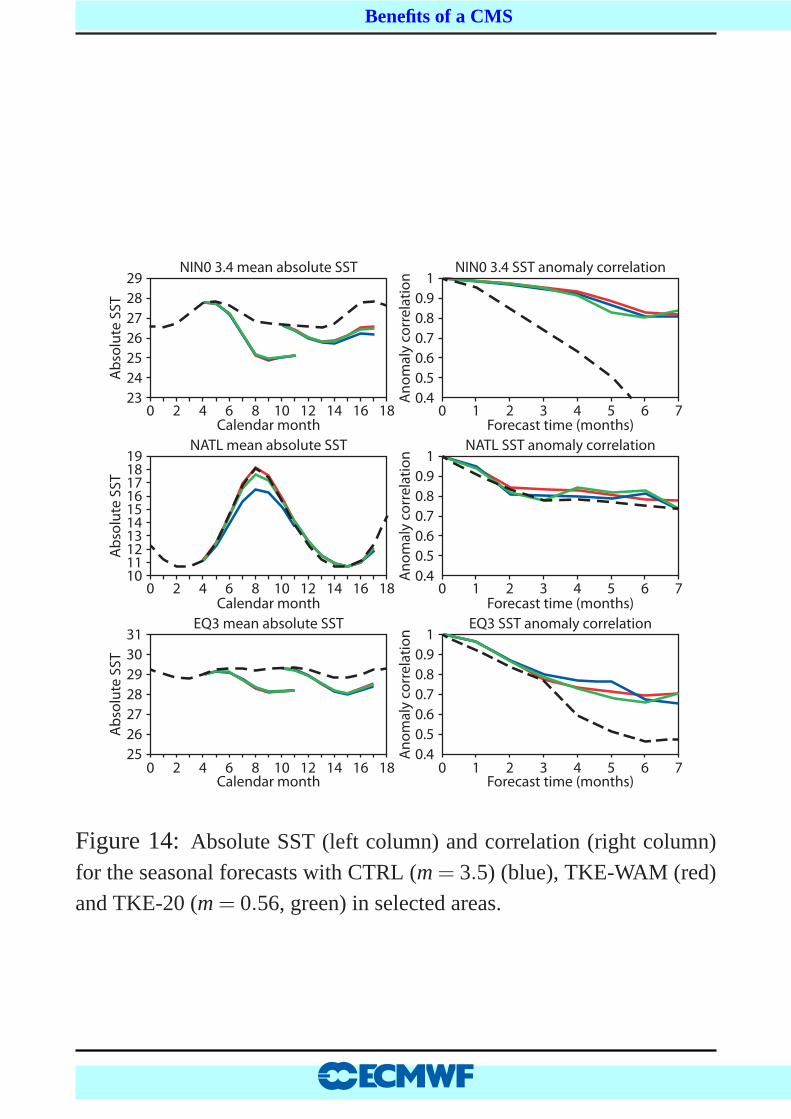
Figure 14:Absolute SST (left column) and correlation (right column)

for the seasonal forecasts with CTRL (m = 3.5) (blue), TKE-WAM (red)

and TKE-20 (m = 0.56, green) in selected areas.

30


COUPLING FROM DAY 0

Presently, in the operational medium-range/monthly ensemble forecasting system

(ENS) the interaction between atmosphere and ocean is only switched on at Day 10 in

the forecast. In the autumn a new version of ENS will be introduced in operations

where the coupling starts from Day 0. Also, sea state effectson upper ocean mixing

and dynamics will be switched on.

Coupling from Day 0 has beneficial impacts on

• hurricane forecasting (already shown)

• the MJO

• and the statistical properties of ENS.

31 .


0

0.1

0.2

0.3

0.4

0.5

0.6

0.7

0.8

0.9

Co

rre

lati

on

151050 20 25 30 35 40 45Forecast range (Days)

MJO Index bivariate correlation

Uncoupled

Coupled

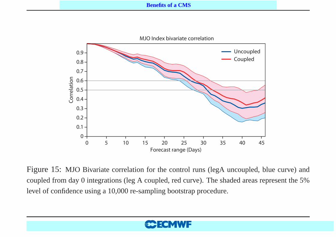
Figure 15:MJO Bivariate correlation for the control runs (legA uncoupled, blue curve) and

coupled from day 0 integrations (leg A coupled, red curve). The shaded areas represent the 5%

level of confidence using a 10,000 re-sampling bootstrap procedure.

32 .


(a) u850hPa, Tropics (b) u850hPa, Tropics

0

1

2

3

4

5(c) u200hPa, Tropics

-0.13

-0.11

-0.09

-0.07

-0.05

-0.03

-0.01

0.01

(d) u200hPa, Tropics

0

0.1

0.2

0.3

0.4

0.5

0.6

(e) t200hPa, Tropics

-0.06

-0.05

-0.04

-0.03

-0.02

-0.01

0

(f) t200hPa, Tropics

129630 15fc-step (d)

129630 15fc-step (d)

CR

PS

CR

PS

129630 15fc-step (d)

129630 15fc-step (d)

CR

PS

CR

PS

129630 15fc-step (d)

129630 15fc-step (d)

CR

PS

CR

PS

-0.04

-0.03

-0.02

-0.01

0

0

1

2

P

C

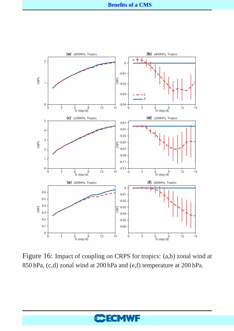
Figure 16:Impact of coupling on CRPS for tropics: (a,b) zonal wind at

850 hPa, (c,d) zonal wind at 200 hPa and (e,f) temperature at 200 hPa.

33


CONCLUSIONS

• There might be a need to have a systematic study on numerics ofcoupled

systems.

• Wave breaking enhances the upper ocean mixing and even affects the average

SST field over a 20 year period, while there is a hint that it might have impact on

predictability.

• There is a trend towards the introduction of more complicated CMS’s. Not only

forecasting but also data assimilation needs to be done in the context of a coupled

system.

• Work on the development of a weakly coupled data assimilation system is in

progress.

34 .

Documents

Ocean circulation and air-sea interaction - ECMWF · Beneﬁts of a CMS. Ocean circulation and air-sea interaction Peter Janssen, Magdalena Balmaseda, Jean Bidlot, Øyvind Breivik,