Occupational Dose Measurement in Interventional Cardiology

Dosimetry Comparison Study

By

Areej Mutwakkil Attom Ahmad

A thesis submitted for partial fulfillment for the Master degree of Science in Physics

Supervised by:

Dr. Ibrahim Abdalrahim Shadad

Physics Department Faculty of Science

University of Khartoum

(May 2008)

Acknowledgement It is far beyond to express my pleasure, my grateful thanks and deep appreciation to

my supervisor Dr. Ibrahim Abdalrahim Shadad who makes things available and

supplied me with all my needs.

My grateful thanks extended to include my head department Safaa Ibrahim Alkhawad

for advising, encouraging and helping me overcoming all difficulties faced.

My deep thanks to my colleagues Eltayeb, Bodour and Amira and to SSDL

department. They spare no efforts, keeping standing by.

My deep thanks extended To Dr. Isam Alhlu and to Dr. Ibrahim Idris for encouraging

and advising.

Thanks to physics department and to Dr. Omer Ibrahim Eid the head department who

paved and smoothed my way.

To Sudan Atomic Energy Commission and to INIS department.

Thanks to all my dear friends and colleagues;

I never forget my dear father who opened my eyes upon life. To him my thanks and

deep appreciation.

All my thanks and gratefulness to my beloved family who provided me with all my

needs, with love and care.

To all those who stood by me. May God bless all those who shed light upon my way. Whatever been done will be grown and planted on the soil of my heart.

All my thanks firstly and lastly to my God

Abstract

The number of cardiology interventional procedures has significantly increased

recently. This is due to the reliability of the diagnostic equipment to diagnose many

heart diseases. In the procedures the x-ray used results in increasing radiation doses to

the staff. The cardiologists and other staff members in interventional cardiology are

usually working close to the area under examination and receive the dose primarily

from scattered radiation from the patient. Therefore workers in interventional

cardiology are expected to receive high doses.

This study overviews the status of occupational exposure at three cardiology centres

at three different hospitals in Khartoum compared with that received by workers at

other medical practices (radiotherapy, nuclear medicine and diagnostic radiology) in

the Institute of Nuclear Medicine and Technology (INMO) at El Gezira.

The TLD HARSHAW 6600 Reader was used in the assessment of effective dose for

Hp (10). Two TLDs were used by each worker at the three cardiology centres, one

worn under a protective apron and the other worn outside and above the apron as

specified by the ICRP. Each worker at the other sections was facilitated with one

dosimeter to be worn on the chest.

The annual doses received by 14 cardiologists, 13 nurses and 9 technologists at the

three cardiology centres were in the range: (0.84 – 4.77), (0.15 – 2.08), (0.32 – 1.10)

mSv respectively. In the INMO the annual doses received by 7 doctors, 5 nurses and

14 technologists were in the range: (0.12 – 0.51), (0.11 – 0.65), (0.03 – 1.39) mSv

respectively.

The results showed that the annual doses received by the workers do not exceed 20

mSv. The study also indicated that doses received by workers in interventional

cardiology, in particular the cardiologists are high compared to that received at the

other medical sections.

الخلاصة

يرجع هذا للتشخيص الجيد لأمراض القلب باستخدام . تلاحظ مؤخرا الزيادة الكبيرة في عدد عمليات قسطرة القلب

ة . القسطرة والأشعة السينية بيا مقارن ة نس املون لجرعات إشعاعية عالي ات يتعرض الع وع من العملي ذا الن في ه

واجدهم بغرفة العملية أثناء إجراء العملية والتي تستخدم فيها برصفائهم في الاستخدامات الطبية الأخرى، وذلك لت

ة . الأشعة السينية لفترات طويلة افات قريب ي مس ة القسطرة يتواجدون عل طبيب القلب والفريق المشارك في عملي

.من المريض الأمر الذي يعرضهم لجرعات إشعاعية من الأشعة المتشتتة من المريض

ا الإشعاعيةر الجرعات أجريت هذه الدراسة لتقدي ا الع ة مراآز التي يتعرض له الخرطوم قسطرة ملون في ثلاث ب

ا ي يتلقاه ك الت ع تل املونم رى الع ة الأخ ات الطبي ي الممارس خيص (-: ف ووي، التش عة، الطب الن لاج بالأش الع

.معهد الطب النووي بالجزيرة في) العلاجي

راءة از الق تخدم جه د ) Harshaw model 6600(اس ي تق ات ف عاعيةير الجرع اس). Hp (10) (الإش لقي

ازين الإشعاعيةالجرعات ة، استخدم آل عامل جه ، TLD التي تعرض لها العاملون في مراآز القسطرة الثلاث

از واحد . فوق الواقي والآخرأحدهما تم تثبيته تحت الواقي الرصاصي م تثبيت جه ووي ت أما في معهد الطب الن

.في الصدر

ا وجد أن الجرعا ي تعرض له درة الت ين في 9 ممرض و 13 طبيب قسطرة، 14ت الإشعاعية السنوية المق تقني

ي ة ف ز القسطرة الثلاث دىمراآ ى ) 1.10 – 0.32(و ) 2.08 – 0.15(، )4.77 – 0.84 (- :الم فرت عل ى س مل

ي تع أما في معهد الطب النووي فقد آانت الجرعات . التوالي ا الإشعاعية السنوية المقدرة الت اء، 7رض له 5 أطب

ي ) 1.39 – 0.03(و ) 0.65 – 0.11( ،)0.51 – 0.12( ما بين المدى تقني في 14ممرضين و ملي سفرت عل

.التوالي

بيا إليتوصلت هذه الدراسة ة نس اء، عالي الأخص الأطب ام القسطرة، ب املون في أقس ا الع ي تلقاه أن الجرعات الت

ارسات الطبية الأخرى آما أثبتت الدراسة أن آل الجرعات الإشعاعية مقارنة بالتي تعرض لها العاملون في المم

ام القلب لا تتعدي يهم أقس ا ف ام بم ذا يتفق مع حد . mSv 20السنوية التي تعرض لها العاملون في آل الأقس ه

.الجرعة السنوي للعاملين في القوانين المحلية والتوصيات العالمية

Contents

Chapter 1 Introduction

Chapter 2 Theoretical Background

2.1. Physics of X-ray 3

2.1.1. Characteristic Radiation or Discrete X-ray Spectrum 4

2.1.2. Bremsstrahlung Radiation or Continuous X-ray Spectrum 4

2.1.3. X-ray Tubes 6

2.1.4. Emission Spectra 7

2.1.5. Properties of X-rays 8

2.2. Interaction of X-rays with Matter 9

2.2.1. Photoelectric effect 9

2.2.2. Compton Effect 9

2.2.3. Pair production 11

2.3. Radiation Quantities and Units 11

2.3.1. Physical Quantities 12

2.3.1.1. Photon Fluence and Energy Fluence 12

2.3.1.2. Kerma 12

2.3.1.3. Absorbed Dose 13

2. 3. 2. Effective Dose 13

2.3.3. Operational Quantities 15

2.4. Occupational Exposure 16

2.5. Use of Personal Monitors to Estimate Effective Dose to Workers for

External Exposure in Interventional Radiology

17

2.6. Reduction of staff doses in Interventional Radiology 18

2.7. Thermoluminescence 19

2.7.1. Thermoluminescence Dosimetry 20

2.7.2. Thermoluminescent Dosimeter Systems 21

2.7.3. Unique Properties of Thermoluminescence 23

2.7.3.1. The Temperature Dimension 23

2.7.3.2. The Colour Dimension 24

2.7.3.3. The Information Content 25

2.7.4. The Glow Curve Analysis 25

2.7.5. Characteristics of TL materials 27

2.7.6. Charge Equilibrium and Filtration 29

2.7.7. Thermoluminescence Signals Caused by Disturbing Effects 30

2.7.7.1. The Teflon Light Emission 30

2.7.7.2. Light Contribution by Additional Heated Materials 30

2.7.8. Applications of TLD 30

Chapter 3 Instrumentation and Experimental Setup

3.1. System Overview 31

3.1.1. WinREMS Application Software 31

3.1.2. TLD Reader 32

3.1.2.1. The Heating System 33

3.1.2.2. The light Detecting System 34

3.1.2.3. The Reference Light Source 35

3.1.3. TLD-100 36

3.2. Secondary Standard Dosimetry Laboratory (SSDL) 37

3.3. Calibration of the Harshaw Reader 37

3.3.1. Calibration Methodology 38

3.3.1.1. Element Correction Coefficients (ECC) 38

3.3.1.2. Reader Calibration Factor (RCF) 40

3.3.2. The Harshaw Reader Calibration 42

3.3.2.1. Generate the calibration cards 42

3.3.2.2. Generate Reader Calibration Factor (RCF) 42

3.3.2.3. Generate Field Cards 43

3.3.2.4. Calibrate the Reader in a Physical Unit 43

3.4. Response Test 43

3.4.1. ICRU Trumpet Curve 43

3.5. Dose Measurement to workers at the three cardiology centres and the

other medical sections

44

Chapter 4 Results and Discussion

4.1. Calibration of Harshaw Reader and TLD cards 46

4.1.1. Generation of Calibration Cards 46

4.1.2. Generation of the Reader Calibration Factor 47

4.1.3. Generation of Field Cards 47

4.1.4. Calibration of the Reader in a physical unit 48

4.2. The Response Test 48

4.3. Effective Dose Measurements to Workers in Interventional Cardiology 50

4.3.1. Hospital 1 51

4.3.2. Hospital 2 54

4.3.3. Hospital 3 47

4.3.4. Comparison of average annual doses received by the workers at the

three centres of cardiology

60

4.4. Doses Measurements to Workers at the Institute of Nuclear Medicine at

El Gezira

61

4.5. Dose Comparison between the cardiology and the other medical

sections

67

Chapter 5 Conclusion and Recommendations

References

List of Figures Figure (2 - 1): Bremsstrahlung Radiation 5

Figure (2 - 2): conventional x-ray tube 6

Figure (2 - 3): Emission spectrum for a tungsten target x-ray tube operated

at 100 kVp. The dotted line represents the theoretical bremsstrahlung. The

solid lin represents the spectrum after self-, inherent, and added filtration.

8

Figure (2 - 4): Photoelectric effect 9

Figure (2 - 5): Compton Effect 10

Figure (2 - 6): Pair production 11

Figure (2 - 7): Electron transitions occurring when thermoluminescent LiF

is irradiated and heated

21

Figure (2 - 8): TLD reader 22

Figure (2 - 9): A typical thermogram (glow curve) of LiF: Mg, Ti measured

with a TLD reader at a low heating rate.

23

Figure (2 - 10): glow curve of a thermoluminescent material 24

Figure (2 - 11): Time Temperature Profile and glow curve for LiF: Mg, Ti

freshly irradiated with 1 Gy

26

Figure (3 - 1): Harshaw TLD Model 6600, Automated TLD Card Reader 33

Figure (3 - 2): TLD card LiF:Mg,Ti 37

Figure (3 - 3): ICRU trumpet curve 44

Figure (4 - 1): ICRU trumpet curve and the responses of the TLDs 50

Figure (4 - 2): Plots of annual doses received by individual workers at

Hospital 1 at the department of cardiology. c – Cardiologist, t –

technologist, n - nurse

53

Figure (4 - 3): Positions of cardiologist (C), nurse (N) and technologist (T)

during examinations

54

Figure (4 – 4): Plots of annual doses received by individual workers at

Hospital 2 at the department of cardiology. c – Cardiologist, t –

technologist, n - nurse

56

Figure (4 - 5): Plots of annual doses received by individual workers at

Hospital 3 at the department of cardiology. c – Cardiologist, t –

technologist, n - nurse

59

Figure (4 - 6): Plots of average annual doses received by the cardiologists,

nurses and technologists at the three centres of cardiology

61

Figure (4 - 7): Plots of annual doses received by individual workers at the

department of radiotherapy. d – Doctor, t – technologist, n - nurse

63

Figure (4 - 8): Plots of annual doses received by individual workers at the

department of nuclear medicine. t – technologist, n - nurse

64

Figure (4 - 9): Plots of annual doses received by individual workers at the

department of diagnostic radiology. d – Doctor, t – technologist, n - nurse

65

Figure (4 - 10): Plots of average annual doses received by the doctors,

nurses and technologists at the three medical sections of radiotherapy,

nuclear medicine and diagnostic radiology in the institute of nuclear

medicine at El Gezira

67

Figure (4 - 11): Plots of average annual doses received by the doctors,

nurses and technologists at the four medical sections of cardiology,

radiotherapy nuclear medicine and diagnostic radiology

69

List of Tables:

Table (2 - 1): Radiation weighting factors (ωR) 14

Table (2 - 2): Tissue weighting factors (ωт) 15

Table(2-3): General Characteristic of Some Commercially Available

Thermoluminescent Dosimeters

28

Table (3 - 1): Properties of TLD-100 material 36

Table (4 – 1): ECC Values of the Golden Cards 47

Table (4 - 2): Response values of the TLD cards 49

Table (4 – 3): Response values of the TLD cards irradiated with x-rays of

different KVp values irradiated with Cs-173

49

Table (4 – 4): Number of cardiologists, nurses and technologists at the three

centres of cardiology

51

Table (4 – 5): Dose Measurements to workers at Hospital 1 - Cardiology

Department

52

Table (4 – 6): Average Annual doses to workers at Hospital 1 – Cardiology

Department

54

Table (4 – 7): Dose Measurements to workers at Hospital 2 – Cardiology

Department

55

Table (4 – 8): Average Annual Doses to workers at Hospital 2 – Cardiology

Department

56

Table (4 – 9): Dose Measurements to workers at Hospital 3 – Cardiology

Department

58

Table (4 – 10): Average Annual Doses to workers at Hospital 3 –

Cardiology Department

59

Table (4 - 11): Average annual doses at the three centres 60

Table (4 - 12): Annual doses of radiotherapy section workers 62

Table (4 - 13): Annual doses of nuclear medicine section workers 63

Table (4 - 14): Annual doses of diagnostic radiology section workers 65

Table (4 - 15): Average annual doses at the three medical sections 66

Table (4 - 16): Average annual doses at the four medical sections 68

Chapter 1

Introduction

Over the last years, increasing application has been made of ionizing radiation in

medical practices. Cardiac catheterization has been used frequently for the evaluation

and treatment with heart diseases. The working staff, particularly cardiologists who

perform these procedures have the highest potential risk of receiving high radiation

doses due to close contact with patients, long time of exposure and complexity of the

procedures.

Interventional cardiology is a branch of the medical specialty of cardiology that

deals specifically with the catheter based treatment of structural heart diseases. A

large number of procedures can be performed on the heart by catheterization. This

most commonly involves the insertion of a sheath into the femoral artery (but, in

practice, any large peripheral artery or vein) and cannulating the heart under X-ray

visualization (most commonly fluoroscopy, a real-time x-ray) [1].

The UNSCEAR 2000 report states that fluoroscopic procedures are by far the largest

source of exposure in medicine. Cardiac catheterization, in particular, can represent a

major source of radiation exposure [2].

Occupational Exposure Control is an important part in the establishment of radiation

protection infrastructure in a country. The individual monitoring, due to external

exposure of ionizing radiation, is the primary procedure to ensure the safety for

radiation workers and to control the doses received at workplace so that not to exceed

the dose limits specified in BSS-115 [3].

There are four cardiology centres in Khartoum. In this study an attempt has been

made to measure doses received by the workers in the cardiology centres and compare

them with those received in other medical practices.

The study was conducted at three cardiac laboratories in three hospitals. The three

laboratories are equipped with C-arm x-ray image intensifier units.

Each worker at these laboratories was facilitated with two Thermoluminescence

Dosimeters (TLDs) to be worn over and under the apron. The doses recorded by the

1

two dosimeters were used to estimate the effective dose as recommended by the ICRP

[4].

The doses received at these cardiology centres were compared with those received at

the medical sections of radiotherapy, nuclear medicine and diagnostic radiology in the

Institute of Nuclear Medicine and Technology (INMO) in El Gezira.

Each worker in these sections was facilitated with one TLD to be worn on the trunk to

measure Hp (10) which estimates the effective dose.

The TLD HARSHAW 6600 Reader was used in the assessment of effective dose for

Hp (10). Firstly, the Harshaw reader and the TLD cards were calibrated using the

Secondary Standard Dosimetry Laboratory (SSDL) at the Sudan Atomic Energy

Commission (SAEC). Then a response test was performed to assess the performance

of the dosimetry system.

This study shows that workers of cardiology, particularly the cardiologists receive

high doses compared with workers in other medical sections. This study focused on

the need to set constant monitoring for the workers to assist in reducing the

occupational exposure.

It is worthwhile to mention here that the study makes a point for authorities to become

cautious for the workers of interventional cardiology, particularly the cardiologists.

Although the doses received by individual workers are well below the allowed limit,

yet need a special care to further strengthen the principle of ALARA (As Low As

Reasonably Achievable).

2

Chapter 2

Theoretical Background

In this chapter the production and properties of x-rays, characteristics and functions of

thermoluminescence are presented.

2.1 Physics of X-ray When fast moving electrons slam into a metal object, x-rays are produced. The kinetic

energy is transformed into electromagnetic energy.

The function of the x-ray machine is to provide a sufficient intensity of electron flow

from the cathode (a filament) to the anode in a controlled manner. The three principal

parts of an x-ray machine are the control panel, a high-voltage power supply, and the

x-ray tube are all designated to provide a large number of electrons focused to a small

spot in such a manner that when electrons arrive at a target, they have acquired a

kinetic energy.

When these projectile electrons impinge on a heavy metallic atom of the target, they

interact with these atoms and transfer its kinetic energy to the target. These

interactions occur within a very small depth of penetration into the target. As they

occur, the projectile electrons slow down and finally come nearly to rest, at which

time they could be conducted through the x-ray anode assembly and out into the

associated electronic circuitry. The projectile electron interacts with either the orbital

electron or the nuclei of target atoms. The interactions result in conversion of kinetic

energy into thermal energy and electro magnetic energy in the form of x-rays as

follows: [5]

)12(21

max2max −=== hvVemvKE

where V is the voltage across the tube, e is the electronic charge, and h is the Plank

constant. Ve represents the energy on which an electron of mass m and velocity v

strikes the target and υmax is the maximum frequency of x-rays [5].

3

2.1.1 Characteristic Radiation or Discrete X-ray Spectrum If the projectile electron interacts with an inner-shell electron of the target atom rather

than outer-shell electron, characteristic radiation can be produced. Characteristic x-ray

results when the interaction is sufficiently violent to ionize the target atom by total

removal of the inner-shell electron. Excitation of an inner-shell electron does not

produce characteristic radiation.

When a target electron ionizes a target atom by removal of a K-shell electron, a

temporary electron hole is produced in the K-shell. This highly unnatural state for the

target atom is corrected by an outer-shell electron falling into the hole in the K-shell.

The transition of an orbital electron from an outer shell to an inner shell is

accompanied by the emission of x-ray photon.

The x-ray has energy equal to the difference in the binding energies of the orbital

electrons involved [5].

)22( −−= BK EEhv

Where h υ is the energy of the x-ray photon, EK and EB are the binding energies of the

orbital electrons respectively.

Since the electron binding energy for every element is different, the characteristic x-

rays produced in the varieties of elements are also different. This type of radiation is

called characteristic radiation because it is characteristic of the target element. The

effective energy of characteristic x-rays increases with increasing atomic number of

the target element [5].

2.1.2 Bremsstrahlung Radiation or Continuous X-ray Spectrum This is a second type of interaction in which the projectile electrons can lose its

kinetic energy as a result of its interaction with the nucleus of a target atom. In this

type of interaction, the kinetic energy of the projectile electron is converted into

electromagnetic energy. A projectile electron that completely avoids the orbital

electrons on passing through an atom of a target may come sufficiently close to the

nucleus of the atom and be under its influence. Since the electron is negatively

charged and the nucleus is positively charged, there is an electrostatic force of

attraction between them. As the projectile electron approaches the nucleus, it is

influenced by a nuclear force much stronger than an electrostatic attraction. As it

passes by the nucleus, it slowed down and deviated in its course, leaving with a

4

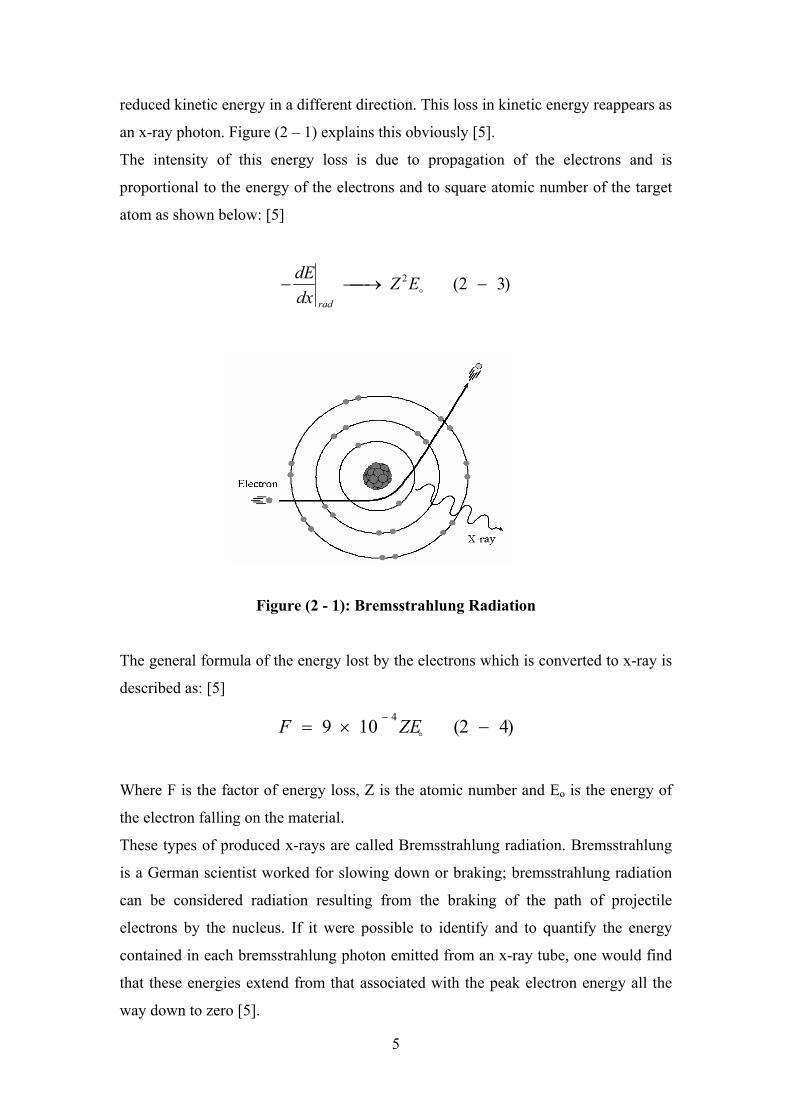
reduced kinetic energy in a different direction. This loss in kinetic energy reappears as

an x-ray photon. Figure (2 – 1) explains this obviously [5].

The intensity of this energy loss is due to propagation of the electrons and is

proportional to the energy of the electrons and to square atomic number of the target

atom as shown below: [5]

)32(2 −⎯→⎯− oEZdxdE

rad

Figure (2 - 1): Bremsstrahlung Radiation

The general formula of the energy lost by the electrons which is converted to x-ray is

described as: [5]

)42(109 4−×=

−

oZEF

Where F is the factor of energy loss, Z is the atomic number and Eo is the energy of

the electron falling on the material.

These types of produced x-rays are called Bremsstrahlung radiation. Bremsstrahlung

is a German scientist worked for slowing down or braking; bremsstrahlung radiation

can be considered radiation resulting from the braking of the path of projectile

electrons by the nucleus. If it were possible to identify and to quantify the energy

contained in each bremsstrahlung photon emitted from an x-ray tube, one would find

that these energies extend from that associated with the peak electron energy all the

way down to zero [5].

5

2.1.3 X-ray Tubes To produce medical images with x-rays, a source is required that:

- Produces enough x rays in a short time

- Allows the user to vary the x-ray energy

- Provides x rays in a reproducible fashion

- Meets standards of safety and economy of operation

In x-ray tubes, bremsstrahlung and characteristic x rays are produced as high-speed

electrons interact in a target. While the physical design of x-ray tubes has been altered

significantly over a century, the basic principles of operation have not changed [6].

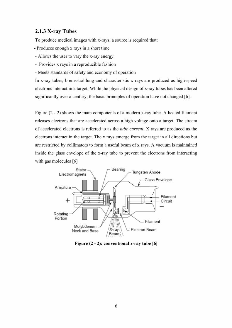
Figure (2 - 2) shows the main components of a modern x-ray tube. A heated filament

releases electrons that are accelerated across a high voltage onto a target. The stream

of accelerated electrons is referred to as the tube current. X rays are produced as the

electrons interact in the target. The x rays emerge from the target in all directions but

are restricted by collimators to form a useful beam of x rays. A vacuum is maintained

inside the glass envelope of the x-ray tube to prevent the electrons from interacting

with gas molecules [6]

Figure (2 - 2): conventional x-ray tube [6]

6

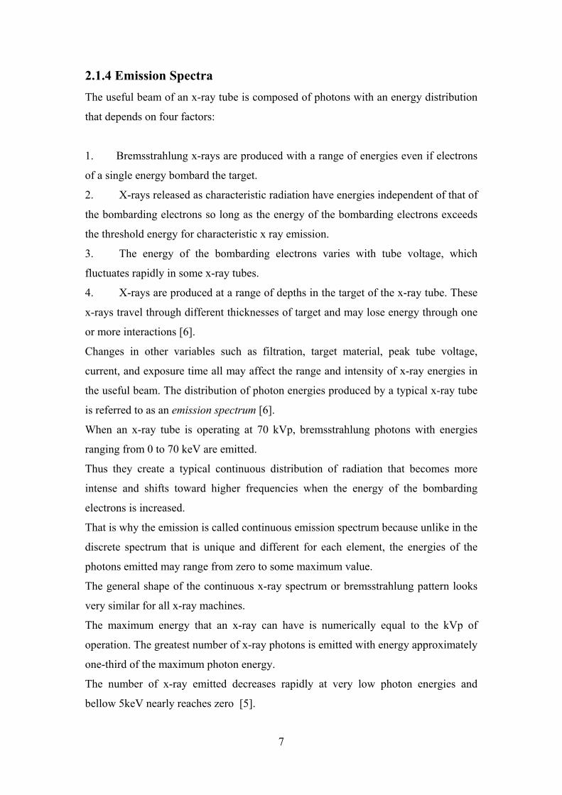
2.1.4 Emission Spectra The useful beam of an x-ray tube is composed of photons with an energy distribution

that depends on four factors:

1. Bremsstrahlung x-rays are produced with a range of energies even if electrons

of a single energy bombard the target.

2. X-rays released as characteristic radiation have energies independent of that of

the bombarding electrons so long as the energy of the bombarding electrons exceeds

the threshold energy for characteristic x ray emission.

3. The energy of the bombarding electrons varies with tube voltage, which

fluctuates rapidly in some x-ray tubes.

4. X-rays are produced at a range of depths in the target of the x-ray tube. These

x-rays travel through different thicknesses of target and may lose energy through one

or more interactions [6].

Changes in other variables such as filtration, target material, peak tube voltage,

current, and exposure time all may affect the range and intensity of x-ray energies in

the useful beam. The distribution of photon energies produced by a typical x-ray tube

is referred to as an emission spectrum [6].

When an x-ray tube is operating at 70 kVp, bremsstrahlung photons with energies

ranging from 0 to 70 keV are emitted.

Thus they create a typical continuous distribution of radiation that becomes more

intense and shifts toward higher frequencies when the energy of the bombarding

electrons is increased.

That is why the emission is called continuous emission spectrum because unlike in the

discrete spectrum that is unique and different for each element, the energies of the

photons emitted may range from zero to some maximum value.

The general shape of the continuous x-ray spectrum or bremsstrahlung pattern looks

very similar for all x-ray machines.

The maximum energy that an x-ray can have is numerically equal to the kVp of

operation. The greatest number of x-ray photons is emitted with energy approximately

one-third of the maximum photon energy.

The number of x-ray emitted decreases rapidly at very low photon energies and

bellow 5keV nearly reaches zero [5].

7

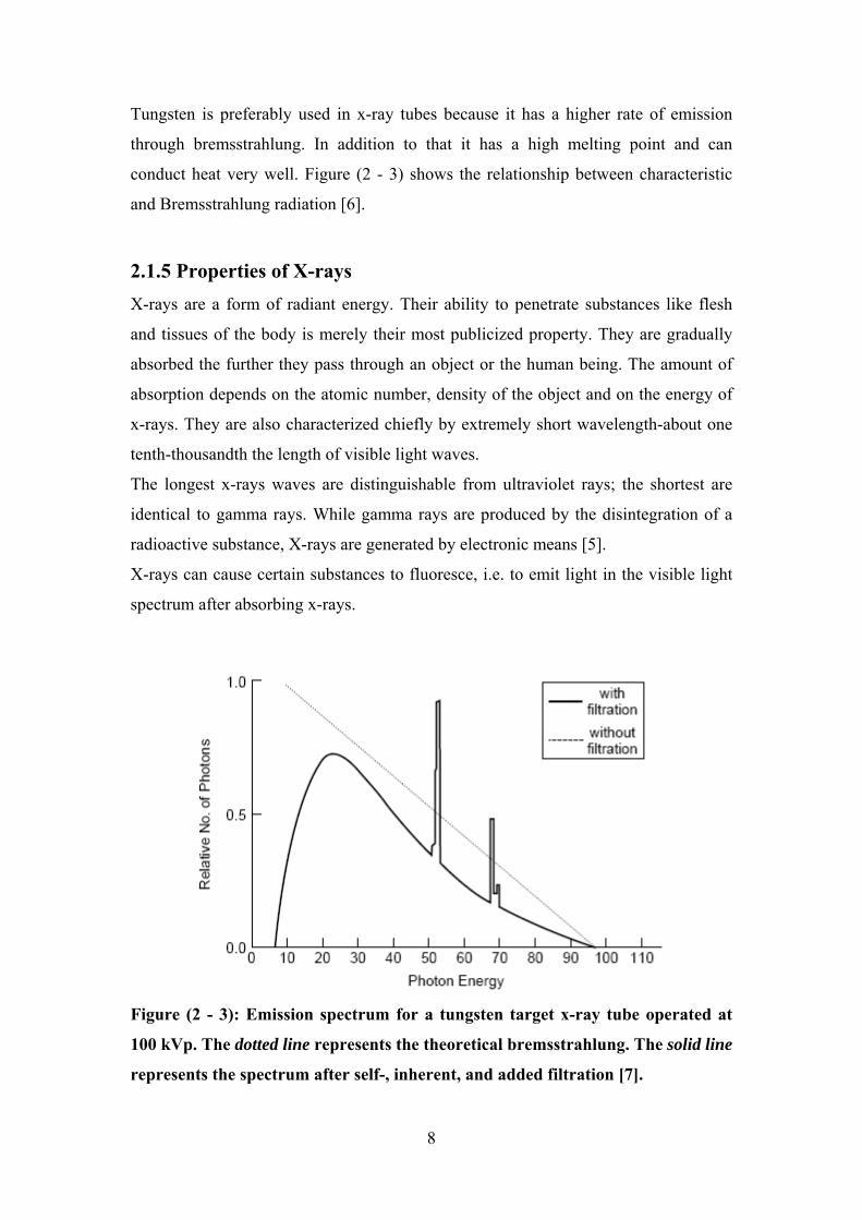
Tungsten is preferably used in x-ray tubes because it has a higher rate of emission

through bremsstrahlung. In addition to that it has a high melting point and can

conduct heat very well. Figure (2 - 3) shows the relationship between characteristic

and Bremsstrahlung radiation [6].

2.1.5 Properties of X-rays X-rays are a form of radiant energy. Their ability to penetrate substances like flesh

and tissues of the body is merely their most publicized property. They are gradually

absorbed the further they pass through an object or the human being. The amount of

absorption depends on the atomic number, density of the object and on the energy of

x-rays. They are also characterized chiefly by extremely short wavelength-about one

tenth-thousandth the length of visible light waves.

The longest x-rays waves are distinguishable from ultraviolet rays; the shortest are

identical to gamma rays. While gamma rays are produced by the disintegration of a

radioactive substance, X-rays are generated by electronic means [5].

X-rays can cause certain substances to fluoresce, i.e. to emit light in the visible light

spectrum after absorbing x-rays.

Figure (2 - 3): Emission spectrum for a tungsten target x-ray tube operated at

100 kVp. The dotted line represents the theoretical bremsstrahlung. The solid line

represents the spectrum after self-, inherent, and added filtration [7].

8

2.2 Interaction of X-rays with Matter

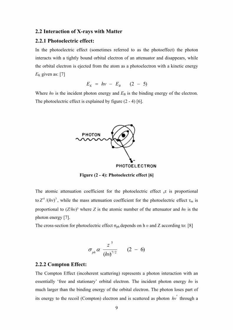
2.2.1 Photoelectric effect: In the photoelectric effect (sometimes referred to as the photoeffect) the photon

interacts with a tightly bound orbital electron of an attenuator and disappears, while

the orbital electron is ejected from the atom as a photoelectron with a kinetic energy

EK given as: [7]

)52( −−= BK EhvE

Where hυ is the incident photon energy and EB is the binding energy of the electron.

The photoelectric effect is explained by figure (2 - 4) [6].

Figure (2 - 4): Photoelectric effect [6]

The atomic attenuation coefficient for the photoelectric effect aτ is proportional

to , while the mass attenuation coefficient for the photoelectric effect τ34 )/(hvZ m is

proportional to (Z/hυ)³ where Z is the atomic number of the attenuator and hυ is the

photon energy [7].

The cross-section for photoelectric effect σph depends on h υ and Z according to: [8]

)62()( 2/7

5

−hvz

phασ

2.2.2 Compton Effect: The Compton Effect (incoherent scattering) represents a photon interaction with an

essentially ‘free and stationary’ orbital electron. The incident photon energy hυ is

much larger than the binding energy of the orbital electron. The photon loses part of

its energy to the recoil (Compton) electron and is scattered as photon through a vh ′

9

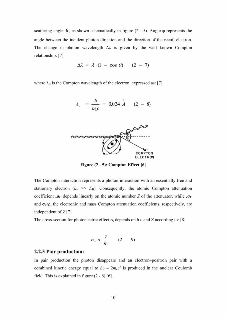
scattering angle , as shown schematically in figure (2 - 5). Angle φ represents the

angle between the incident photon direction and the direction of the recoil electron.

The change in photon wavelength ∆λ is given by the well known Compton

relationship: [7]

θ

)72()cos1( −−=Δ θλλ c

where λC is the Compton wavelength of the electron, expressed as: [7]

)82(024.0 −==o

Acm

h

ec

λ

Figure (2 - 5): Compton Effect [6]

The Compton interaction represents a photon interaction with an essentially free and

stationary electron (hυ >> EB). Consequently, the atomic Compton attenuation

coefficient aσC depends linearly on the atomic number Z of the attenuator, while eσC

and σC/ρ, the electronic and mass Compton attenuation coefficients, respectively, are

independent of Z [7].

The cross-section for photoelectric effect σc depends on h υ and Z according to: [8]

)92( −hvZ

c ασ

2.2.3 Pair production: In pair production the photon disappears and an electron–positron pair with a

combined kinetic energy equal to hυ – 2mec² is produced in the nuclear Coulomb

field. This is explained in figure (2 - 6) [6].

10

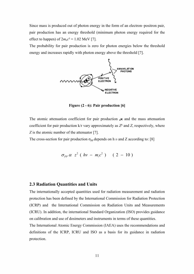
Since mass is produced out of photon energy in the form of an electron–positron pair,

pair production has an energy threshold (minimum photon energy required for the

effect to happen) of 2mec² = 1.02 MeV [7].

The probability for pair production is zero for photon energies below the threshold

energy and increases rapidly with photon energy above the threshold [7].

Figure (2 - 6): Pair production [6]

The atomic attenuation coefficient for pair production aκ and the mass attenuation

coefficient for pair production k/r vary approximately as Z² and Z, respectively, where

Z is the atomic number of the attenuator [7].

The cross-section for pair production σpp depends on h υ and Z according to: [8]

)102()( 22 −− cmhvzPP oασ

2.3 Radiation Quantities and Units The internationally accepted quantities used for radiation measurement and radiation

protection has been defined by the International Commission for Radiation Protection

(ICRP) and the International Commission on Radiation Units and Measurements

(ICRU). In addition, the international Standard Organization (ISO) provides guidance

on calibration and use of dosimeters and instruments in terms of these quantities.

The International Atomic Energy Commission (IAEA) uses the recommendations and

definitions of the ICRP, ICRU and ISO as a basis for its guidance in radiation

protection.

11

2.3.1 Physical Quantities:

2.3.1.1 Photon Fluence and Energy Fluence: These quantities are usually used to describe photon beams and may also be used in

describing charged particle beams [7].

The particle fluence Φ is the quotient dN by dA, where dN is the number of particles

incident on a sphere of cross-sectional area dA: [7]

)112( −=dAdNφ

The unit of particle fluence is m²־.

The energy fluence ψ is the quotient of dE by dA, where dE is the radiant energy

incident on a sphere of cross-sectional area dA: [7]

)122( −=dAdEψ

The unit of energy fluence is J/m² [7].

2.3.1.2 KERMA: KERMA is an acronym for kinetic energy released per unit mass. It is a nonstochastic

quantity applicable to indirectly ionizing radiations such as photons and neutrons. It

quantifies the average amount of energy transferred from indirectly ionizing radiation

to directly ionizing radiation without concern as to what happens after this transfer

[7].

The kerma is defined as the mean energy transferred from the indirectly ionizing

radiation to charged particles (electrons) in the medium dĒtr per unit mass dm: [7]

)132( −=dmEd

K tr

The unit of kerma is joule per kilogram (J/kg). The name for the unit of kerma is the

gray (Gy), where 1 Gy = 1 J/kg [7].

12

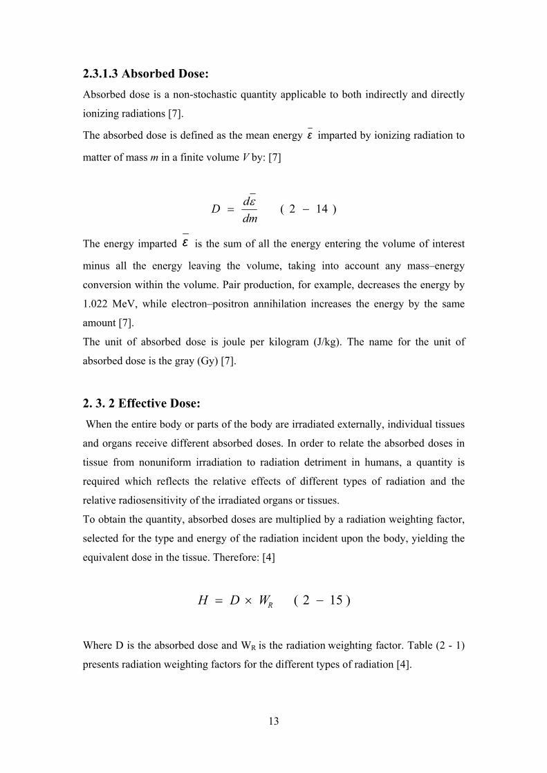
2.3.1.3 Absorbed Dose: Absorbed dose is a non-stochastic quantity applicable to both indirectly and directly

ionizing radiations [7].

The absorbed dose is defined as the mean energy ε imparted by ionizing radiation to

matter of mass m in a finite volume V by: [7]

)142( −=dmdD ε

The energy imparted ε is the sum of all the energy entering the volume of interest

minus all the energy leaving the volume, taking into account any mass–energy

conversion within the volume. Pair production, for example, decreases the energy by

1.022 MeV, while electron–positron annihilation increases the energy by the same

amount [7].

The unit of absorbed dose is joule per kilogram (J/kg). The name for the unit of

absorbed dose is the gray (Gy) [7].

2. 3. 2 Effective Dose: When the entire body or parts of the body are irradiated externally, individual tissues

and organs receive different absorbed doses. In order to relate the absorbed doses in

tissue from nonuniform irradiation to radiation detriment in humans, a quantity is

required which reflects the relative effects of different types of radiation and the

relative radiosensitivity of the irradiated organs or tissues.

To obtain the quantity, absorbed doses are multiplied by a radiation weighting factor,

selected for the type and energy of the radiation incident upon the body, yielding the

equivalent dose in the tissue. Therefore: [4]

)152( −×= RWDH

Where D is the absorbed dose and WR is the radiation weighting factor. Table (2 - 1)

presents radiation weighting factors for the different types of radiation [4].

13

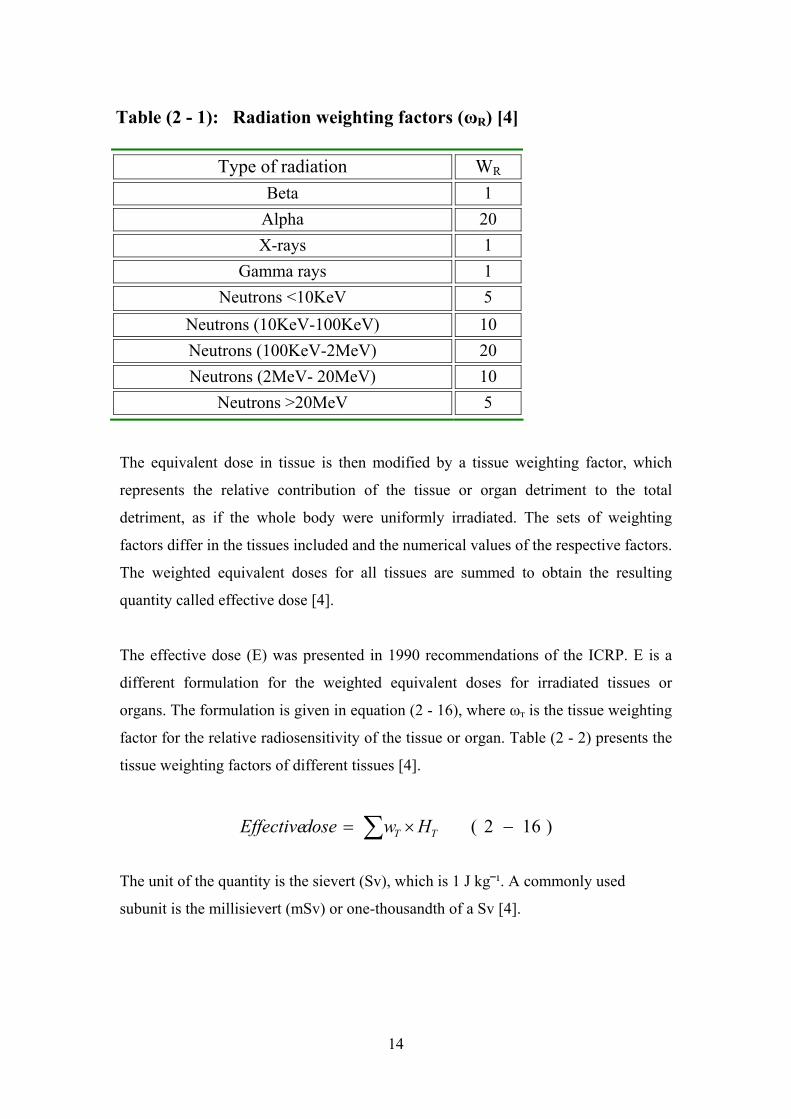
Table (2 - 1): Radiation weighting factors (ωR) [4]

Type of radiation WR

Beta 1 Alpha 20 X-rays 1

Gamma rays 1 Neutrons <10KeV 5

Neutrons (10KeV-100KeV)

10

Neutrons (100KeV-2MeV) 20 Neutrons (2MeV- 20MeV) 10

Neutrons >20MeV 5

The equivalent dose in tissue is then modified by a tissue weighting factor, which

represents the relative contribution of the tissue or organ detriment to the total

detriment, as if the whole body were uniformly irradiated. The sets of weighting

factors differ in the tissues included and the numerical values of the respective factors.

The weighted equivalent doses for all tissues are summed to obtain the resulting

quantity called effective dose [4].

The effective dose (E) was presented in 1990 recommendations of the ICRP. E is a

different formulation for the weighted equivalent doses for irradiated tissues or

organs. The formulation is given in equation (2 - 16), where ωт is the tissue weighting

factor for the relative radiosensitivity of the tissue or organ. Table (2 - 2) presents the

tissue weighting factors of different tissues [4].

)162( −×= ∑ TT HwdoseEffective

The unit of the quantity is the sievert (Sv), which is 1 J kg⎯¹. A commonly used

subunit is the millisievert (mSv) or one-thousandth of a Sv [4].

14

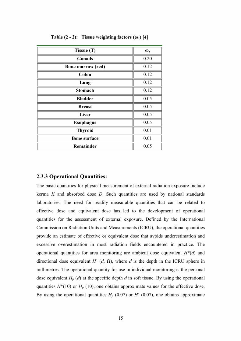
Table (2 - 2): Tissue weighting factors (ωт) [4]

Tissue (T) ωт

Gonads 0.20 Bone marrow (red) 0.12 Colon 0.12 Lung 0.12

Stomach 0.12

Bladder 0.05 Breast 0.05

Liver 0.05

Esophagus

0.05 Thyroid 0.01

Bone surface 0.01 Remainder 0.05

2.3.3 Operational Quantities: The basic quantities for physical measurement of external radiation exposure include

kerma K and absorbed dose D. Such quantities are used by national standards

laboratories. The need for readily measurable quantities that can be related to

effective dose and equivalent dose has led to the development of operational

quantities for the assessment of external exposure. Defined by the International

Commission on Radiation Units and Measurements (ICRU), the operational quantities

provide an estimate of effective or equivalent dose that avoids underestimation and

excessive overestimation in most radiation fields encountered in practice. The

operational quantities for area monitoring are ambient dose equivalent H*(d) and

directional dose equivalent H΄ (d, Ω), where d is the depth in the ICRU sphere in

millimetres. The operational quantity for use in individual monitoring is the personal

dose equivalent Hp (d) at the specific depth d in soft tissue. By using the operational

quantities H*(10) or Hp (10), one obtains approximate values for the effective dose.

By using the operational quantities Hp (0.07) or H΄ (0.07), one obtains approximate

15

values for the equivalent dose to the skin. Similarly, Hp (3) or H΄ (3) may be used for

an approximate assessment of the equivalent dose to the lens of the eye [9].

2.4 Occupational Exposure The BSS defines occupational exposure as: “All exposures of workers incurred in the

course of their work, with the exception of exposures excluded from the Standards

and exposures from practices or sources exempted by the Standards [9].

Evaluation of radiation dose received by the workers is referred to as personal

monitoring and it plays an essential role in the protection of occupational radiation

workers. It measures the quantity of radiation to which a worker is exposed through

the use of thermo-luminescent dosimeter (TLD)/film badge. The TLD is one of the

common devices used to estimate the level of radiation exposure to a worker.

It is well known that occupational doses of radiation in interventional procedures

guided by fluoroscopy are the highest doses registered among medical staff using x

rays. Interventional cardiologists represent the most important group of medical

specialists involved in such practices [10].

Occupational dosimetry is critical for the personal safety of interventionists. The

ICRP and the ACC recommend the use of two personal dosimeters, one worn outside

the apron at the left shoulder or neck and the other worn under the apron at the waist

[10].

The personal dose equivalent at 10 mm depth, Hp (10), is used to provide an estimate

of effective dose for comparison with the appropriate dose limits. As Hp (0.07) is

used to estimate the equivalent dose to skin, it should be used for extremity

monitoring, where the skin dose is the limiting quantity [11].

The limits on effective dose for occupational exposure apply to the sum of effective

doses from external sources and committed effective doses from intakes in the same

period:

(a) an effective dose of 20 mSv per year averaged over five consecutive years;

(b) an effective dose of 50 mSv in any single year;

(c) an equivalent dose to the lens of the eye of 150 mSv in a year; and

16

(d) an equivalent dose to the extremities (hands and feet) or the skin of 500 mSv in a

year [9].

2.5 Use of personal monitors to estimate effective dose to workers for

external exposure in interventional radiology Clinical staff taking part in diagnostic and interventional procedures using

fluoroscopy wears protective aprons to shield internal tissues and organs in the torso

from scattered x-ray. Use of the measurements from monitoring devices worn outside

and above protective aprons as the record of E for these individuals results in

significant overestimates of their actual risk [4].

When two dosimeters are used, one worn under a protective apron at the waist or on

the chest [where HW is HP (10) value for this personal monitor] and the other worn

outside and above the apron at the neck [where HN is Hp (10) value for this

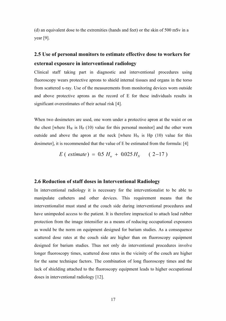
dosimeter], it is recommended that the value of E be estimated from the formula: [4]

)172(025.05.0)( −+= Nw HHestimateE

2.6 Reduction of staff doses in Interventional Radiology In interventional radiology it is necessary for the interventionalist to be able to

manipulate catheters and other devices. This requirement means that the

interventionalist must stand at the couch side during interventional procedures and

have unimpeded access to the patient. It is therefore impractical to attach lead rubber

protection from the image intensifier as a means of reducing occupational exposures

as would be the norm on equipment designed for barium studies. As a consequence

scattered dose rates at the couch side are higher than on fluoroscopy equipment

designed for barium studies. Thus not only do interventional procedures involve

longer fluoroscopy times, scattered dose rates in the vicinity of the couch are higher

for the same technique factors. The combination of long fluoroscopy times and the

lack of shielding attached to the fluoroscopy equipment leads to higher occupational

doses in interventional radiology [12].

17

Moreover patients undergoing interventional radiology procedures tend to require

more staff in the room for clinical support. Thus other doctors such as anesthetists and

nursing staff may also be present during a procedure.

In view of the high occupational dose levels it is important to ensure that staff is

monitored adequately. Interventionalists and others who stand at the couchside should

be provided with one or more dosimeters to wear. One dosimeter, generally worn at

the waist level under a lead apron, will be issued to monitor whole body or effective

dose. In some countries whole body dose is monitored using a dosimeter at collar

level worn above the lead apron. Staff may also be issued with additional dosimeters

to assess the equivalent dose to critical organs such as the eyes or hands. Hand dose

may be monitored using small thermoluminescent dosimeters worn under rubber

gloves.

Unfortunately, wearing a single dosimeter does not give a good indication of effective

dose. A combination of two dosimeter readings, one above the apron and one below

will yield an improved estimate of effective dose [12].

Local action levels are a useful means of limiting staff doses in interventional

radiology. The reason for the higher than usual dosimeter reading should be

established and action taken to minimize the individual's dose. These action levels are

set some way below the levels at which the individual would be classified. These

action levels serve to identify individuals who may receive higher than normal doses

and enable the radiation protection service to implement an action plan to reduce staff

doses. This action plan could involve staff training or a review of protective measures.

The use of local action levels serves as a constraint on occupational exposures. They

are not dose constraints in the true meaning of the definition given by ICRP [12].

Scattered radiation dose-rates at the couchside during fluoroscopy procedures can be

quite high. However, dose-rates decrease rapidly with increasing distance away from

the couch, approximately obeying an inverse square law with the reference point

being the centre of the field on the patient. Taking one step back from the couch can

have a dramatic effect on the radiation dose to the individual [12].

18

2.7 Thermoluminescence Thermoluminescence is thermally activated phosphorescence; it is the most

spectacular and widely known of a number of different ionizing radiation induced

thermally activated phenomena. Its practical applications range from archaeological

pottery dating to radiation dosimetry. A useful phenomenological model of the

thermoluminescence mechanism is provided in terms of the band model for solids.

The storage traps and recombination centres, each type characterized with an

activation energy (trap depth) that depends on the crystalline solid and the nature of

the trap, are located in the energy gap between the valence band and the conduction

band. The states just below the conduction band represent electron traps, the states

just above the valence band are hole traps. The trapping levels are empty before

irradiation (i.e. the hole traps contain electrons and the electron traps do not). During

irradiation the secondary charged particles lift electrons into the conduction band

either from the valence band (leaving a free hole in the valence band) or from an

empty hole trap (filling the hole trap) [7].

The system may approach thermal equilibrium through several means:

- Free charge carriers recombine with the recombination energy converted into heat;

- A free charge carrier recombines with a charge carrier of opposite sign trapped at a

luminescence centre, the recombination energy being emitted as optical

fluorescence;

- The free charge carrier becomes trapped at a storage trap, and this event is then

responsible for phosphorescence or the thermoluminescence and optical stimulated

luminescence (OSL) processes [7].

2.7.1 Thermoluminescence Dosimetry

Diagramed in Figure (2 - 7) are energy levels for electrons within crystals of a

thermoluminescent material such as LiF. Electrons “jump” from the valence band to

the conduction band by absorbing energy from ionizing radiation impinging upon the

crystals. Some of the electrons return immediately to the valence band; other are

“trapped” in intermediate energy levels supplied by impurities in the crystals. The

number of electrons trapped in intermediate levels is proportional to the energy

absorbed by the LiF phosphor during irradiation. Only rarely do electrons escape from

the traps and return directly to the ground state. Unless energy is supplied for their

19

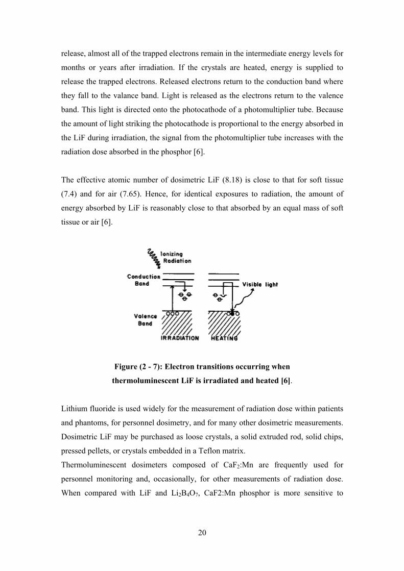
release, almost all of the trapped electrons remain in the intermediate energy levels for

months or years after irradiation. If the crystals are heated, energy is supplied to

release the trapped electrons. Released electrons return to the conduction band where

they fall to the valance band. Light is released as the electrons return to the valence

band. This light is directed onto the photocathode of a photomultiplier tube. Because

the amount of light striking the photocathode is proportional to the energy absorbed in

the LiF during irradiation, the signal from the photomultiplier tube increases with the

radiation dose absorbed in the phosphor [6].

The effective atomic number of dosimetric LiF (8.18) is close to that for soft tissue

(7.4) and for air (7.65). Hence, for identical exposures to radiation, the amount of

energy absorbed by LiF is reasonably close to that absorbed by an equal mass of soft

tissue or air [6].

Figure (2 - 7): Electron transitions occurring when

thermoluminescent LiF is irradiated and heated [6].

Lithium fluoride is used widely for the measurement of radiation dose within patients

and phantoms, for personnel dosimetry, and for many other dosimetric measurements.

Dosimetric LiF may be purchased as loose crystals, a solid extruded rod, solid chips,

pressed pellets, or crystals embedded in a Teflon matrix.

Thermoluminescent dosimeters composed of CaF2:Mn are frequently used for

personnel monitoring and, occasionally, for other measurements of radiation dose.

When compared with LiF and Li2BB4O7, CaF2:Mn phosphor is more sensitive to

20

ionizing radiation; however, the response of this phosphor varies rapidly with photon

energy [6].

2.7.2 Thermoluminescent Dosimeter Systems The TLDs most commonly used in medical applications are LiF: Mg, Ti,

LiF:Mg,Cu,P and Li2BB4O7:Mn, because of their tissue equivalence. Other TLDs, used

because of their high sensitivity, are CaSO4:Dy, Al2O3:C and CaF2:Mn. In this work

LiF:Mg,Ti TLDs were used.

- TLDs are available in various forms (e.g. powder, chips, rods and ribbons).

- Before they are used, TLDs need to be annealed to erase the residual signal. Well

established and reproducible annealing cycles, including the heating and cooling

rates, should be used.

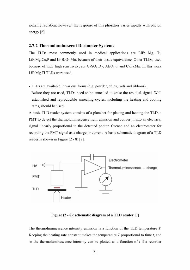
A basic TLD reader system consists of a planchet for placing and heating the TLD, a

PMT to detect the thermoluminescence light emission and convert it into an electrical

signal linearly proportional to the detected photon fluence and an electrometer for

recording the PMT signal as a charge or current. A basic schematic diagram of a TLD

reader is shown in Figure (2 - 8) [7].

Figure (2 - 8): schematic diagram of a TLD reader [7]

The thermoluminescence intensity emission is a function of the TLD temperature T.

Keeping the heating rate constant makes the temperature T proportional to time t, and

so the thermoluminescence intensity can be plotted as a function of t if a recorder

21

output is available with the TLD measuring system. The resulting curve is called the

TLD glow curve. In general, if the emitted light is plotted against the crystal

temperature one obtains a thermoluminescence thermogram Figure (2 - 9). [3]

The peaks in the glow curve may be correlated with trap depths responsible for

thermoluminescence emission.

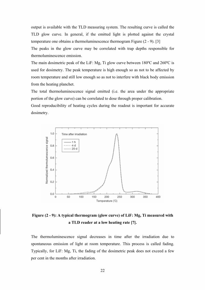
The main dosimetric peak of the LiF: Mg, Ti glow curve between 180ºC and 260ºC is

used for dosimetry. The peak temperature is high enough so as not to be affected by

room temperature and still low enough so as not to interfere with black body emission

from the heating planchet.

The total thermoluminescence signal emitted (i.e. the area under the appropriate

portion of the glow curve) can be correlated to dose through proper calibration.

Good reproducibility of heating cycles during the readout is important for accurate

dosimetry.

Figure (2 - 9): A typical thermogram (glow curve) of LiF: Mg, Ti measured with

a TLD reader at a low heating rate [7].

The thermoluminescence signal decreases in time after the irradiation due to

spontaneous emission of light at room temperature. This process is called fading.

Typically, for LiF: Mg, Ti, the fading of the dosimetric peak does not exceed a few

per cent in the months after irradiation.

22

The thermoluminescence dose response is linear over a wide range of doses, although

it increases in the higher dose region, exhibiting supralinear behaviour before it

saturates at even higher doses [7].

TLDs need to be calibrated before they are used (thus they serve as relative

dosimeters). To derive the absorbed dose from the thermoluminescence reading a few

correction factors have to be applied, such as those for energy, fading and dose

response non-linearity [7].

2.7.3 Unique Properties of Thermoluminescence:

2.7.3.1 The Temperature Dimension: The systematic observation of TL involves the continuous measurement of varying

intensity of light output as material is progressively heated. During the measurement,

the heat input is controlled to produce a constant rate of temperature increase, so that

the temperature rise is proportional to the time that has elapsed since the start of the

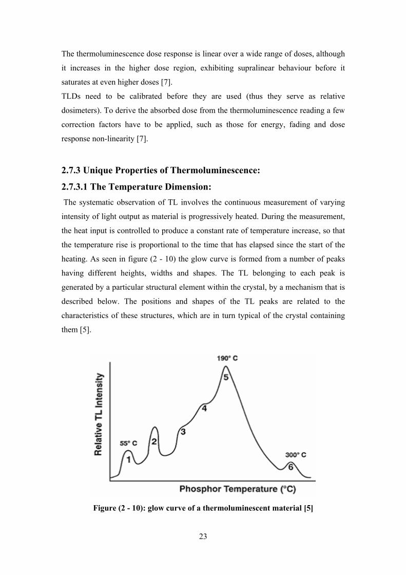
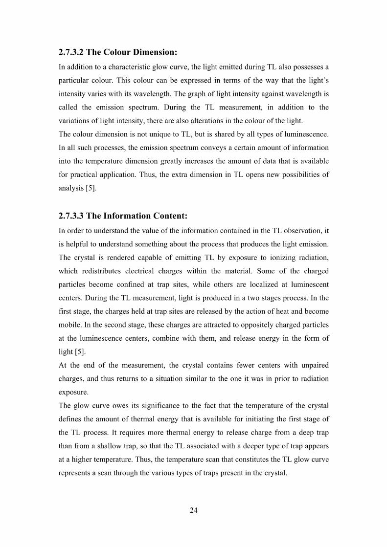
heating. As seen in figure (2 - 10) the glow curve is formed from a number of peaks

having different heights, widths and shapes. The TL belonging to each peak is

generated by a particular structural element within the crystal, by a mechanism that is

described below. The positions and shapes of the TL peaks are related to the

characteristics of these structures, which are in turn typical of the crystal containing

them [5].

Figure (2 - 10): glow curve of a thermoluminescent material [5]

23

2.7.3.2 The Colour Dimension: In addition to a characteristic glow curve, the light emitted during TL also possesses a

particular colour. This colour can be expressed in terms of the way that the light’s

intensity varies with its wavelength. The graph of light intensity against wavelength is

called the emission spectrum. During the TL measurement, in addition to the

variations of light intensity, there are also alterations in the colour of the light.

The colour dimension is not unique to TL, but is shared by all types of luminescence.

In all such processes, the emission spectrum conveys a certain amount of information

into the temperature dimension greatly increases the amount of data that is available

for practical application. Thus, the extra dimension in TL opens new possibilities of

analysis [5].

2.7.3.3 The Information Content: In order to understand the value of the information contained in the TL observation, it

is helpful to understand something about the process that produces the light emission.

The crystal is rendered capable of emitting TL by exposure to ionizing radiation,

which redistributes electrical charges within the material. Some of the charged

particles become confined at trap sites, while others are localized at luminescent

centers. During the TL measurement, light is produced in a two stages process. In the

first stage, the charges held at trap sites are released by the action of heat and become

mobile. In the second stage, these charges are attracted to oppositely charged particles

at the luminescence centers, combine with them, and release energy in the form of

light [5].

At the end of the measurement, the crystal contains fewer centers with unpaired

charges, and thus returns to a situation similar to the one it was in prior to radiation

exposure.

The glow curve owes its significance to the fact that the temperature of the crystal

defines the amount of thermal energy that is available for initiating the first stage of

the TL process. It requires more thermal energy to release charge from a deep trap

than from a shallow trap, so that the TL associated with a deeper type of trap appears

at a higher temperature. Thus, the temperature scan that constitutes the TL glow curve

represents a scan through the various types of traps present in the crystal.

24

By contrast, the colour of light emitted is determined, in the second stage of the TL

process, by the type of luminescence centre where the charges combine. Since the

form of the glow curve is related to the charge traps, and the emission spectrum is

determined by the luminescence centers, the TL measurement provides information

about both stages of the luminescence process simultaneously [5].

2.7.4 The Glow Curve Analysis The light output from the TL material is collected by a photomultiplier tube (PMT)

during the heating up procedure and using adequate electronics it can be visualized

and integrated. The time temperature profile (TTP) influences the shape of the glow

curve as it is seen in Figure (2 - 11). The location of the glow peaks along the

temperature axis depends on heating rate [5].

Sometimes if the heating rate is linear, instead of the temperature, the heat up time is

used to characterize the glow curve.

Therefore the read out procedure should be regulated in such a way that the complete

glow curve is obtained during the linear section of the TTP. Here it can be observed

also that even in the same material the number of peaks (i.e. the number of energy

bands of the crystal) depends on the presence of the (artificial or natural) impurities

(doping elements). The electrons trapped in lowest energy band (releasable at low

temperature) can easily disappear without extra heating as it is explained by the

diffusion theory, but it takes time. Consequently, each energy band has a lifetime, and

this procedure (called fading) causes loss of information. By mathematical procedures

(called deconvolution) each peak of the glow curve can be separated. From the above

mentioned facts it is evident that the ratios of integrals of separated glow peaks reflect

the energy spectrum of the photons immediately after the exposure and the change in

ratios depend on the life-time of the peak considered. With the knowledge of the half-

life this phenomenon can be utilized to determine the time of the exposure before the

read out procedure [5].

25

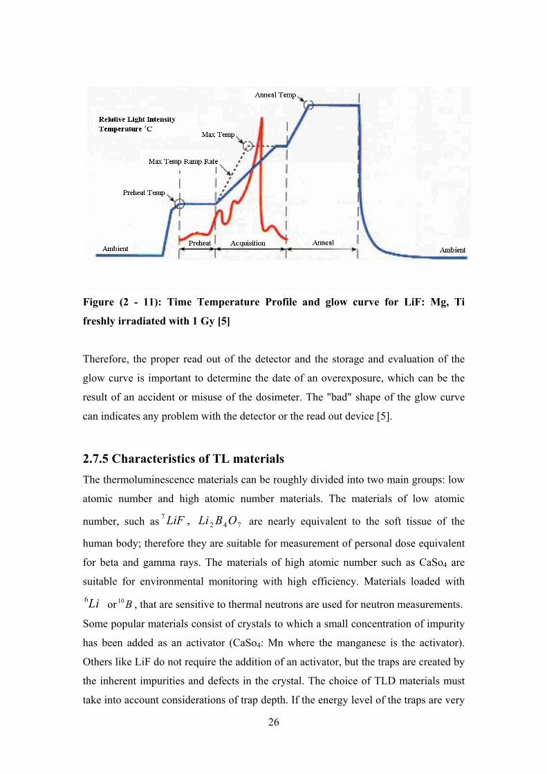
Figure (2 - 11): Time Temperature Profile and glow curve for LiF: Mg, Ti

freshly irradiated with 1 Gy [5]

Therefore, the proper read out of the detector and the storage and evaluation of the

glow curve is important to determine the date of an overexposure, which can be the

result of an accident or misuse of the dosimeter. The "bad" shape of the glow curve

can indicates any problem with the detector or the read out device [5].

2.7.5 Characteristics of TL materials The thermoluminescence materials can be roughly divided into two main groups: low

atomic number and high atomic number materials. The materials of low atomic

number, such as are nearly equivalent to the soft tissue of the

human body; therefore they are suitable for measurement of personal dose equivalent

for beta and gamma rays. The materials of high atomic number such as CaSo

7427 , OBLiLiF

4 are

suitable for environmental monitoring with high efficiency. Materials loaded with

orLi6 B10 , that are sensitive to thermal neutrons are used for neutron measurements.

Some popular materials consist of crystals to which a small concentration of impurity

has been added as an activator (CaSo4: Mn where the manganese is the activator).

Others like LiF do not require the addition of an activator, but the traps are created by

the inherent impurities and defects in the crystal. The choice of TLD materials must

take into account considerations of trap depth. If the energy level of the traps are very

26

near to the edge of band gap (as in CaSo4: Mn), the number of trap carriers per unit

exposure can be very large. The shallow traps are somewhat unstable even at ordinary

room temperature, however, and therefore the material will show a considerable

"fading" which can loose as much as 85% of the trapped carriers over a few days

time. Therefore, other materials such as CaF2: Mn and LiF: Mg, Ti, with somewhat

deeper traps, are better suited for longer-terms even though their sensitivity is several

orders of magnitude less [5].

General characteristics of some commercially available TL materials are summarized

in Table (2 - 3).

The dose range covered partly depends upon the kind of TLD. Generally, the dose

range of TLD with high atomic number extends from 10 µSv to several hundreds of

mSv and the TLD of the low atomic number cover a range from 0.1 mSv to several Sv

[5].

For TLD materials with higher atomic number, the enhanced photoelectric interaction

probably exaggerates the response to low-energy X-rays and gamma rays. However,

the construction of the TLD reader can largely influence these values. In particular

mostly multi-element personal dosimeters are used: 2 or 4 elements in a card

combined with filter containing holders. The advantages of using multi-element type

TLDs are:

- Able to measure a greater range of doses

- Doses may be easily obtained

- They can be read on site instead of being sent away for developing

- Quicker turnaround time for readout

- Reusable

27

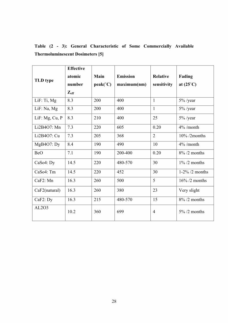
Table (2 - 3): General Characteristic of Some Commercially Available

Thermoluminescent Dosimeters [5]

TLD type

Effective

atomic

number

Zeff

Main

peak(˚C)

Emission

maximum(nm)

Relative

sensitivity

Fading

at (25˚C)

LiF: Ti, Mg 8.3 200 400 1 5% /year

LiF: Na, Mg 8.3 200 400 1 5% /year

LiF: Mg, Cu, P 8.3 210 400 25 5% /year

Li2B4O7: Mn 7.3 220 605 0.20 4% /month

Li2B4O7: Cu 7.3 205 368 2 10% /2months

MgB4O7: Dy 8.4 190 490 10 4% /month

BeO 7.1 190 200-400 0.20 8% /2 months

CaSo4: Dy 14.5 220 480-570 30 1% /2 months

CaSo4: Tm 14.5 220 452 30 1-2% /2 months

CaF2: Mn 16.3 260 500 5 16% /2 months

CaF2(natural) 16.3 260 380 23 Very slight

CaF2: Dy 16.3 215 480-570 15 8% /2 months

AL2O3

10.2 360 699 4 5% /2 months

28

The disadvantages of using multi-element TLDs are:

- Each dose cannot be readout more than once

- The readout process effectively "zeros" the TLD

TLD manufacturing differs from company to company, so specific chip arrangement

and composition may vary. Most badges are lithium fluoride (LiF) and calcium

fluoride (CaF).

Lithium has two stable isotopes, and . Neutron dosimeters use which is

often made with the TLD-700 chip for its sensitivity to beta and gamma rays. The

TLD-600 chip is made with , which is sensitive to neutrons [5].

Li6 Li7 LiF7

LiF6

2.7.6 Charge Equilibrium and Filtration: The sensitivity of a TL material, i.e. the integrated light output after a given exposure

depends on the type of the material, the photon energy and on the presence of other

materials which may release electrons external to and captured by the TL material.

The TL material can be made thick enough to ensure the majority of the electrons

released by the radiation remain captured within the TL material or in other words:

charge equilibrium is fulfilled [5].

The sensitivity of a given material can be modified by external components (filters).

These materials can help to establish the charge equilibrium meanwhile the thickness

of TL material is decreasing.

Beside this effect there will be a possibility of energy discrimination. High energy

photons (having a long mean free path) can easily escape both the filters and the TL

material without producing electrons, or the high energy electrons released will not be

trapped in the TL material.

The other effect of the filter is to absorb low energy electrons emitted within the filter.

Without a filter the low energy photons, having a high cross section for the

photoelectric effect and Compton scattering, produce enough low energy electrons

which will be trapped within the TL material, thus the response is high. However,

when the photon energy is high, then owing to the long mean free path of photons and

high energy of the small amount of electrons, which may or may not escape from the

material, the response will be essentially smaller. A thick filtration absorbs the

majority of low energy photons but the high energy photons produce large number of

29

electrons by Compton scattering or pair production interactions, to ensure charge

equilibrium [5].

2.7.7 Thermoluminescence Signals Caused by Disturbing Effects:

2.7.7.1 The Teflon Light Emission: A signal received when heating the Teflon, which contributes to the TL signal. During

the heating of the TLD phosphors, some effects can cause spurious signals in the TL

range (which are not due to radiation exposure). When evaluating low doses, these

effects can be significant and they must be taken into consideration [5].

Horowtiz pointed out that the light induced TL emission from the Teflon has a glow

peak at 120 degrees Celsius (test should be done for the glow curve with the Teflon,

without the crystal) [5].

The amount of light emission is dependent on the storage condition of the TLD cards.

If the cards were exposed to light, the emission is larger [5].

2.7.7.2 Light Contribution by Additional Heated Materials: Materials present on the TLD cards/crystals/ such as dirt or other contamination

during the readout process may contribute to the light output. The influence can be

recognized in the shape of the glow curves and sometimes can be separated from the

exposure information [5].

2.7.8 Applications of TLD: TLDS are used extensively in wide ranges of application on which have special

requirement. Some of these are as follows:

- Personal monitoring

- Environmental dosimeter (require high sensitivity)

- Patient dosimeter in radiotherapy and x-ray diagnosis (requiring wide dose ranges)

- Military dosimeter (requiring special dosimeters and the use of portable instruments)

[5].

30

Chapter 3

Materials and Method

This chapter describes the Harshaw TLD Reader used for the measurements,

equipments and calibration procedures for the Harshaw Reader and the TLD cards

used in this study for the assessment of occupational doses in interventional

cardiology.

3.1 System Overview The Harshaw Model 6600 Automated TLD Card Reader Workstation is a fully

automated, state-of-the-art instrument used for extremity, environmental and whole

body thermoluminescence dosimetry (TLD) measurement. It combines a medium

capacity (200 TLD Cards or Carrier Cards) transport system with a non-contact

heating system for accurate and reproducible measurements with a minimum of

operator attention required.

The system consists of two major components: the TLD Reader and the Windows

Radiation Evaluation and Management System (WinREMS) software resident on a

personal computer (PC), which is connected to the Reader via a serial

communications port.

3.1.1 WinREMS Application Software

The data architecture of the system includes both a host computer in the Reader and a

Windows-based PC connected through an RS-232-C serial communication port. The

dosimetry functions are divided between the Reader and the Harshaw WinREMS

(Windows Radiation Evaluation and Management System) software on the PC. All

dosimetric data storage, instrument control, and operator inputs are performed on the

PC; transport subsystem control, the gas, vacuum controls, signal acquisition and

conditioning are performed in the Reader. Sufficient redundancy is maintained that

dosimetric data is never lost in the event of a power failure.

WinREMS controls the operations of the Reader, including storing the operating

parameters: Time Temperature Profiles (TTPs), Reader Calibration Factors (RCFs),

31

and Element Correction Coefficients (ECCs). The flexible design of WinREMS

enables the user to automatically calibrate the reader and the dosimeters in a wide

variety of dosimetric units, or to work directly in nanocoulombs and do his own

calibration through a custom spreadsheet program.

As the Reader generates TL data, the host computer stores it until a reading is

completed. It then transmits the data to WinREMS in the form of 200 response points

forming a glow curve. WinREMS displays the curve as it is received and then stores

the data for future computation and reporting. WinREMS also performs a variety of

calibration and Quality Assurance operations.

The user may create, store, and select from any number of Time Temperature Profiles

(TTPs) and Acquisition Setup Parameters. A separate reader Calibration Factor (RCF)

can be established for each TTP to assure accurate conversion of data from charge to

dosimetric units [13].

3.1.2 TLD Reader The heating system uses a stream of hot nitrogen gas at precisely controlled, linearly

ramped temperatures to simultaneously heat one or two card positions. Four-chip

cards are read by automatically executing two sequential acquisition-heating cycles

without removing and reloading the cards. The hot gas heating and the superior

electronic design produce consistent and repeatable glow curves over a wide dynamic

range. The non-contact heating extends card life, enabling many more readings and

longer life for each TLD card.

The operator interface of the Reader is menu-driven and is controlled by seven

pushbuttons on the front panel of the instrument. The Start and Stop pushbuttons

control the Reader's operation. Results of all read operation, including glow curves

and computed data, are displayed on an electroluminescent panel. Figure (3 - 1)

shows Harshaw TLD Reader Model 6600.

The method of reading a TL detector is simple. In a relatively short time (usually

ranging from a few seconds to a few minutes) the TLD is heated from ambient

temperature to some 200-300 ºC, and the emitted light is measured quantitatively.

Thus the reader consists essentially of two basic parts:

A heating device

And a light detecting system

32

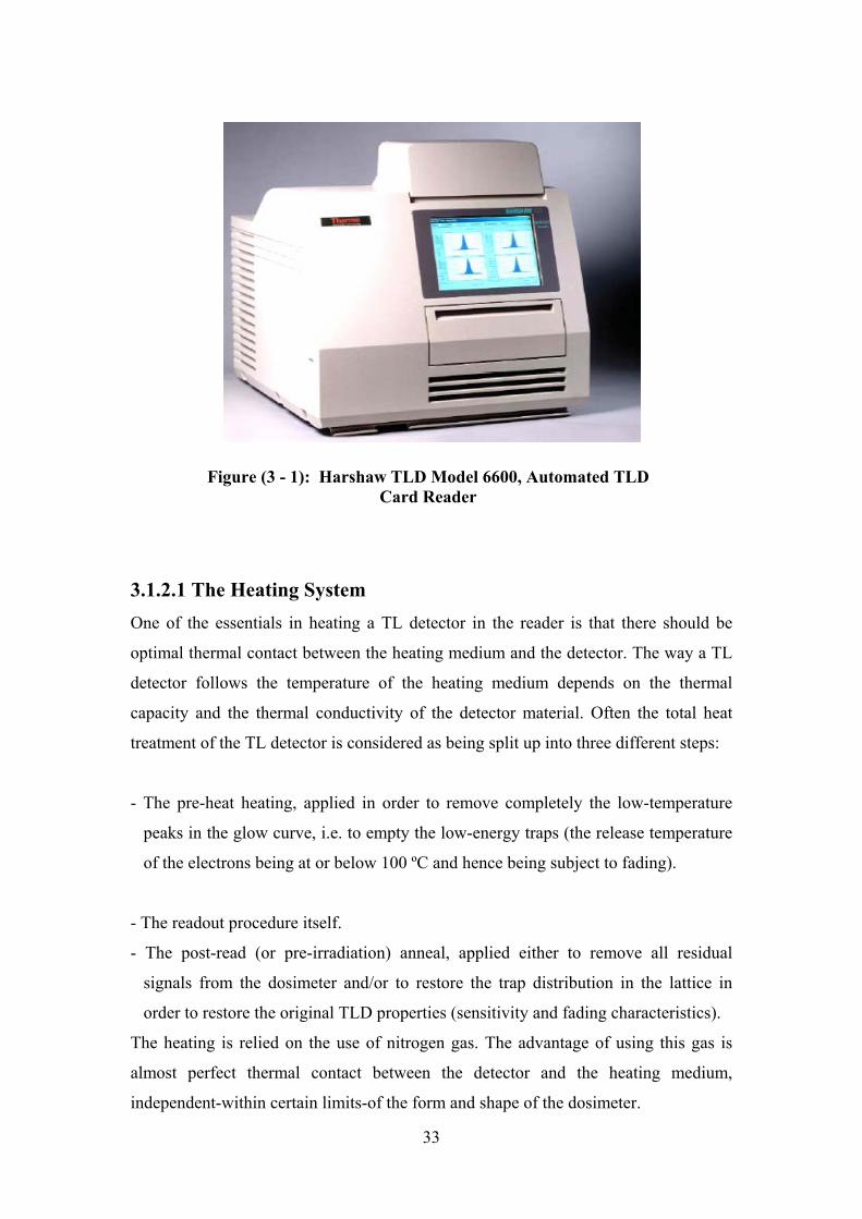
Figure (3 - 1): Harshaw TLD Model 6600, Automated TLD Card Reader

3.1.2.1 The Heating System One of the essentials in heating a TL detector in the reader is that there should be

optimal thermal contact between the heating medium and the detector. The way a TL

detector follows the temperature of the heating medium depends on the thermal

capacity and the thermal conductivity of the detector material. Often the total heat

treatment of the TL detector is considered as being split up into three different steps:

- The pre-heat heating, applied in order to remove completely the low-temperature

peaks in the glow curve, i.e. to empty the low-energy traps (the release temperature

of the electrons being at or below 100 ºC and hence being subject to fading).

- The readout procedure itself.

- The post-read (or pre-irradiation) anneal, applied either to remove all residual

signals from the dosimeter and/or to restore the trap distribution in the lattice in

order to restore the original TLD properties (sensitivity and fading characteristics).

The heating is relied on the use of nitrogen gas. The advantage of using this gas is

almost perfect thermal contact between the detector and the heating medium,

independent-within certain limits-of the form and shape of the dosimeter.

33

3.1.2.2 The light Detecting System The light detecting system does not affect the TL detector during readout as the

heating system does and therefore this part of the reader has less to do with the pitfalls

of thermoluminescence dosimeter. The general task of the light detecting system is to

convert the light emitted by the TL detector into an electronic signal (current, charge,

voltage) which can be measured and activate output devices (printer, computer, etc).

The light detecting system can be thought of as being divided into three parts:

1. The light collecting system

2. The light detector and signal amplifier

3. The signal conditioning system

1. The light Collecting System Detectors with high efficiency are able to concentrate as much luminescence light as

possible on the sensitive layer of the light detector. It would in principle be efficient to

bring the TLD into direct contact with the photocathode.

However, because of the temperature sensitivity of the photocathode, thermal

separation is necessary. To achieve this, several methods have been applied. Using

lens systems, heat filters etc.

2. The light Detecting and the Signal Amplifier A PM tube is chosen for measuring the quantity of radiation absorbed by the TL

material. It is made in such a way that its wavelength typical of the TL material under

consideration.

As an example, emits in the blue-green region, whereas emits in the

red. For optimal results, these materials require different PM tubes. Sensitivity and

signal-to-noise ratio are affected by a number of parameters. Some of them are now

dealt with briefly.

LiF 742 OBLi

- Dark Current: Is the signal which is generated by the PMT while light is absent. The phenomenon

is mainly due to thermal emission of electrons from the cathode layer. PM tubes,

even of the same type, may show large variations in dark current, a reason why they

34

preferably selected for low noise. The remaining dark current is kept as low as

possible by operating the tube at low temperature.

- Fatigue Effects: If the PMT is exposed to large light intensities, its sensitivity decreases, while the

dark current increases.

- Aging Effects: After long use the gain of the PMT gradually decreases. In addition to long-term

gain drift, a slow shift in spectral response may occur. With calibration a correction

factor can be added.

3. The signal Conditioning System The signal conditioning system essentially services to convert the PM signal into a

quantity which can be measured quantitatively. The PM signal (which is typically a

picoamp level) generally needs further amplification.

3.1.2.3 The Reference Light Source The many sources of error discussed in the previous subsections make frequent

sensitivity checks of the entire system a matter of necessity.

For a more consistent test of the sensitivity, one test is carried by using a reference

constant light source.

The source is placed near the normal position of the TLD. The test is done before

each reading or at suitable intervals. If correctly applied, this method of system

'calibration' may trace changes in the optical pathway, change in PM sensitivity and

malfunction of the electronic circuitry. Reference light source measurements have

been used for automatic checks of the overall system sensitivity.

Light sources are usually made of usually made of long-lived radio-isotopes (

or ) embedded in scintillation material.

C14

Sr90

Light emitted by the source should preferably have the same spectral composition as

that of the TLD material in use. Errors can be introduced due to changes in light

sources itself or variations in the spectral response of the photomultiplier tube.

35

3.1.3 TLD - 100 The TLD dosimeter that is used for occupational exposure assessment consists of a

TLD card containing two elements of TLD-100 chips (Lithium Fluoride) , doped with

Mg, Ti, encapsulated between 2 sheets of Teflon 0.0025 inches (10mg/cm²) thick,

mounted on an aluminum sheet of 4cm x 3cm. The two chips have different

thicknesses, 0.38mm and 0.15mm, placed on locations (ii) and location (iii) of the

card respectively as illustrated in figure (3 - 2).

The TLD card is used with a holder. The holder of the TLD card is a badge with

standard filters for providing different radiation absorption and estimation of Hp(10)

and Hp(0.07) (deep body and surface body dose).

The personal dose equivalent at 10 mm depth, Hp(10), is used to provide an estimate

of effective dose for comparison with the appropriate dose limits [11].

For workers in interventional radiology, who use two TLDs under and above the

apron, it is recommended to use equation (2 - 17) to estimate the effective dose [4].

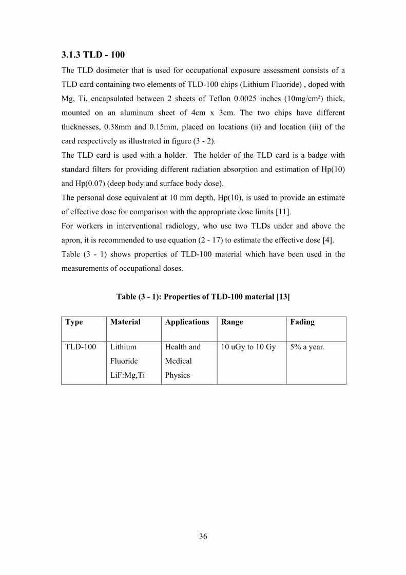
Table (3 - 1) shows properties of TLD-100 material which have been used in the

measurements of occupational doses.

Table (3 - 1): Properties of TLD-100 material [13]

Fading Range Applications Material Type

5% a year. 10 uGy to 10 Gy Health and

Medical

Physics

Lithium

Fluoride

LiF:Mg,Ti

TLD-100

36

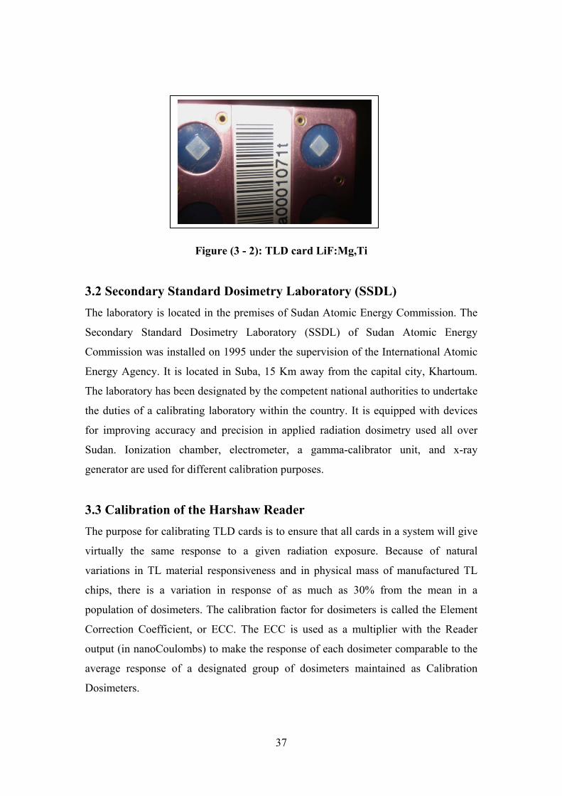
Figure (3 - 2): TLD card LiF:Mg,Ti

3.2 Secondary Standard Dosimetry Laboratory (SSDL) The laboratory is located in the premises of Sudan Atomic Energy Commission. The

Secondary Standard Dosimetry Laboratory (SSDL) of Sudan Atomic Energy

Commission was installed on 1995 under the supervision of the International Atomic

Energy Agency. It is located in Suba, 15 Km away from the capital city, Khartoum.

The laboratory has been designated by the competent national authorities to undertake

the duties of a calibrating laboratory within the country. It is equipped with devices

for improving accuracy and precision in applied radiation dosimetry used all over

Sudan. Ionization chamber, electrometer, a gamma-calibrator unit, and x-ray

generator are used for different calibration purposes.

3.3 Calibration of the Harshaw Reader The purpose for calibrating TLD cards is to ensure that all cards in a system will give

virtually the same response to a given radiation exposure. Because of natural

variations in TL material responsiveness and in physical mass of manufactured TL

chips, there is a variation in response of as much as 30% from the mean in a

population of dosimeters. The calibration factor for dosimeters is called the Element

Correction Coefficient, or ECC. The ECC is used as a multiplier with the Reader

output (in nanoCoulombs) to make the response of each dosimeter comparable to the

average response of a designated group of dosimeters maintained as Calibration

Dosimeters.

37

The purpose of Reader calibration is to maintain a consistent output from the Reader

over a period of time based time based on a convenient local source. By using a set of

Calibration Dosimeters and a consistent local source, the Reader's performance may

be kept at a constant level in spite of a high voltage changes, repairs, dirt

accumulation, or long term drift. The calibration factor for Readers is known as the

Reader Calibration Factor, or RCF. This factor converts the raw charge data from the

photomultiplier tube (in nanoCoulombs) to dosimetric units (rems, for example) or

generic units (gU) for input to an algorithm. The two factors are applied according to

the following formula: [13]

)13(arg−

×=

RCFechECCExposure

3.3.1 Calibration Methodology Here definitions and some calculations to determine the ECC and RCF performed by

the WinREMs software are introduced.

3.3.1.1 Element Correction Coefficients (ECC) Since not all TL dosimeters can be manufactured to have exactly the same TL

efficiency (where TL efficiency (TLE) is defined as the emitted TL light intensity per

unit absorbed dose), individual Element Correction Coefficients (ECCs) must be

defined, developed and applied. A typical batch of TL dosimeters has a variation in

TL efficiency of 10-15 % (one relative standard deviation). This spread can be

reduced to 1-2 % by application of ECCs [13].

Let the TL Response (TL Response) of a specific dosimeter be defined as the

measured quantity that results from subjecting the dosimeter to one unit of a given

ionizing radiation. If we could count every single photon emitted by the TLD and

express the units of the ionizing radiation in terms of dose, the TL Response would be

equal to the TL efficiency. Normally such a relationship is not the case; the measured

quantity is usually expressed in units of charge. The TL Response of the dosimeter is,

in general, proportional to the TL efficiency, i.e.:

)23( −×= TLEKTLR

when k is the proportionality constant.

38

Assume all the Calibration Dosimeters are subjected to a quantity L of ionizing

radiation from a given source, where L can be expressed in any convenient unit, for

example, time of irradiation [13].

Let ECCj be the Element Correction Coefficient for dosimeter j (j = 1, 2….., m, where

m is the number of Calibration Dosimeters), and let TLEj and TLRj be the TL

efficiency and the TL response of dosimeter j, respectively. By definition then

)33( −=j

j TLE

TLEECC

When )43(11

−×= ∑=

=

mj

jjTLE

mTLE

With the aid of (3 - 2), (3 - 3) and (3 - 4) can be written in the form

)53( −=TLR

TLRECCj

When )63(11

−×= ∑=

=

mj

jjTLR

mTLR

If Q j is defined as the charge reported by the reader for dosimeter j following its

subjection to n irradiation unit, then TLR j and TLR can be written in the form: [13]

)73( −=nQTLRj

And )83( −=nQ

TLR

39

when )93(11

−×= ∑=

=

mj

jjQ

mQ

Using (3 - 7), (3 - 8) and (3 - 9), (3 - 5) can be written in the form: [13]

)103( −=j

j QQ

ECC

when <Q> is given by (3 - 9) [13].

3.3.1.2 Reader Calibration Factor (RCF) For the Reader to be able to consistently convert stored TL information to measurable

electric signals (charge), it is convenient to express the ratio between the average TL

response of the Calibration Dosimeters and the delivered radiation quantity L in terms

of one variable. Since the numerical value of this variable will be mainly dependent

on the condition of the Reader at a given date and time, it is appropriate to call this

variable Reader Calibration Factor (RCF). The value of the RCF, although not

expressed yet in terms of "real" dose units, provide the main link between TL

response in terms of charge or counts and the absorbed dose or dose equivalent in

term of Gray or Sievert, respectively [13].

The )113( −=LQ

RCF

where <Q> is the average reported charge of a set of Calibration Dosimeters exposed

to a known quantity of radiation L. The unit gU (generic unit) is defined as the unit

which expresses the quantity L. For example, 1 gU can be equal to the amount of

irradiation delivered during a period of one second by a specific source and geometry,

here referred to as the local source or reference source.

Now, the ECCs for the Field Dosimeters can be expressed in terms of the RCF using

(3 - 11): )123( −×

=j

j qLRCFECC

From (3 - 12), L can be expressed in terms of the RCF, ECC and q:

40

)133( −×

=RCF

ECCqL jj

Once ECCs for Calibration Dosimeters and Field Dosimeters have been generated and

the local unit , gU, has been defined, the link to a calibrated source located at a

calibration laboratory should be established .The calibration laboratory is able to

perform the irradiations and report, the delivered quantity in terms of the desired

quantity (for example, dose, dose-equivalent, exposure, etc). A subset of the

calibration dosimeters in their holders is exposed to dose D from a calibrated source

(for example ) and read out [13]. Cs137

The Reader reports its findings in units of gU using (3 - 13); however, since the value

of D as reported by the calibration laboratory is known, one can establish the

following relationships between the local units, gU, and the dose in units of Gy (or

any other quantity with the appropriate unit): [13]

)143( −=DLK

for the gU to dose conversion factor.

Note that K is expressed in units of gU/Gy and provides the link between the local

source and the calibration laboratory in similar way that the RCF value provides the

link between the internal units of the Reader (Counts or charge) and the local source.

For charge integration systems, the RCF is expressed in units of nC/gU, the quantity

RCF*K is expressed in terms of nC/Sievert and provides the link between the internal

units of the Reader and the dose D j [13].

)153( −×

×=

KRCFECCq

Djj

j

3.3.2 The Harshaw Reader Calibration

The heating treatment of the TLD cards starts at preheat temperature of 50 oC

for 0 s at a heating rate of 25 oC/s up to a maximum temperature of 300 oC

within reading time of 13.3 s. The effective deep dose Hp(10) and shallow dose

Hp(0.07) were calculated taking into account the RCF and the ECC.

To calibrate the TLD system the following steps were done:

41

3.3.2.1 Generate the calibration cards In order to calibrate the TLD reader, a group of cards must be carefully selected

according to their ECCs. These cards are known as calibration cards or golden cards.

295 TLD cards were irradiated for 30 seconds with the internal irradiator 90Sr. The

cards were then read to generate the calibration cards. The ECCs are determined using

equation (3 - 10). To select the golden cards the ECC range fed to the reader was

(0.97 – 1.03).

3.3.2.2 Generate Reader Calibration Factor (RCF) The procedure of calibrating the reader consists of adjusting the factors which used to

convert the light output (Q) from the TLD and the TLD reading in units of mSv as

output by the reader. This involved obtaining a Reader calibration Factor (RCF) for

the TLD reader.

To generate the RCF, the golden cards were irradiated with the internal irradiator 90Sr

for to the same time (30 s) to receive the same dose and later read in the form of

charges.

The RCF is found by dividing the measured charge by the quantity of radiation given

to the dosimeter (gU), using equation (3 - 11) [13].

3.3.2.3 Generate Field Cards Field cards distributed to individuals to measure external exposure must be calibrated

to determine their ECCs since TLD crystals have different sensitivities.

The TLD cards were irradiated with the internal irradiator 90Sr for the same time (30

s) to receive the same dose. The ECCs of the field cards were determined using

equation (3 - 12). The ECC range fed to the reader to select the field cards was (0.7 –

1.30).

3.3.2.4 Calibrate the Reader in a Physical Unit For the reader to measure the dose in terms of a physical unit (mSv or mGray), the

calibration cards inserted into holders and attached to a water phantom were irradiated

on the SSDL of SAEC to a known dose. Later they were read in the reader. The dose

delivered to the calibration cards on the SSDL was fed to the reader. Using this RCF

and the ECC values the dose can be calculated by equation (3 - 15).

42

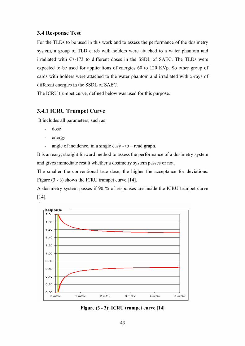
3.4 Response Test For the TLDs to be used in this work and to assess the performance of the dosimetry

system, a group of TLD cards with holders were attached to a water phantom and

irradiated with Cs-173 to different doses in the SSDL of SAEC. The TLDs were

expected to be used for applications of energies 60 to 120 KVp. So other group of

cards with holders were attached to the water phantom and irradiated with x-rays of

different energies in the SSDL of SAEC.

The ICRU trumpet curve, defined below was used for this purpose.

3.4.1 ICRU Trumpet Curve It includes all parameters, such as

- dose

- energy

- angle of incidence, in a single easy - to – read graph.

It is an easy, straight forward method to assess the performance of a dosimetry system

and gives immediate result whether a dosimetry system passes or not.

The smaller the conventional true dose, the higher the acceptance for deviations.

Figure (3 - 3) shows the ICRU trumpet curve [14].

A dosimetry system passes if 90 % of responses are inside the ICRU trumpet curve

[14].

Figure (3 - 3): ICRU trumpet curve [14]

43

3.5 Dose Measurement to workers at the three cardiology centres and

the other medical sections: 92 TLD cards with holders were distributed to workers at three cardiology centres in

three different hospitals. Each worker at the three centres was facilitated with two

dosimeters, to be worn under the apron (at the waist) and above the apron (at the neck

or the collar level), as recommended by the ICRP. The wearing period was one

month.

Five control cards were kept to estimate the background dose during the month

period, for each of the three centres.

After the month period the TLDs were collected to be read in the Harshaw reader

6600.

The background dose recorded for each centre was subtracted from doses recorded by

dosimeters under and above the apron. Then the Effective dose as, recommended by

the ICRP, was estimated from the two readings recorded by dosimeters under and

above the apron using equation (2 - 17).

The annual doses were estimated on the basis of 46 weeks (45 days leave per year).

The annual doses received by the workers in cardiology were compared with those

received by workers at the medical sections of radiotherapy, nuclear medicine and

diagnostic radiology in the Institute of Nuclear Medicine (INMO) at El Gezira.

30 cards with holders were distributed to the workers at the INMO. Each worker was

facilitated with one TLD do be worn on chest to estimate the effective doses. Every

two months the TLDs were collected to be read in the Harshaw reader. 4 readings

were recorded in the eight months period for each worker.

Five control cards were kept to estimate the background during two months period.

This background value was subtracted from all the each two months reading.

The annual dose was then estimated on the basis of 46 weeks (45 days leave per year).

44

Chapter 4

Results and Discussion

This chapter demonstrates the results of calibration of TLD Reader and TLD cards,

linearity and response tests that were carried on the SSDL lab. It also describes the

occupational radiation doses received by the workers at three cardiology centres at

three hospitals compared with that received by the workers at other medical sections

of radiotherapy, nuclear medicine and diagnostic radiology at the Institute of Nuclear

Medicine at El Jezira.

4.1 Calibration of Harshaw Reader and TLD cards: The Reader and the dosimeters were first calibrated. Calibrations were performed

using the Radiation Evaluation and Management System, Win-REMS software

package for dosimeters and Harshaw 6600 Reader with a computer.

The heating treatment of the TLD cards starts at preheat temperature of 50 oC for 0 s

at a heating rate of 25 oC/s up to a maximum temperature of 300 oC within reading

time of 13.3 s. The effective deep dose Hp (10) and shallow dose Hp (0.07) were

calculated taking into account the RCF and the ECC.

Different operation modes were used to generate and maintain reader and dosimeter

calibration factor as specified below:

4.1.1 Generation of Calibration Cards In order to calibrate the TLD Reader, a group of cards, known as calibration cards or

golden cards, were carefully selected for this calibration.

According to the procedures of calibrations mentioned in chapter 3, 295 TLD cards

were irradiated for 30 seconds with the internal irradiator 90Sr. The cards were then

read to generate the calibration cards. The element correction coefficient (ECC) range

used to select the calibration cards was (0.97 - 1.03). Among the 295 TLD cards only

8 were selected as golden cards. Table (4 - 1) shows the accepted values of ECCs for

the golden cards.

45

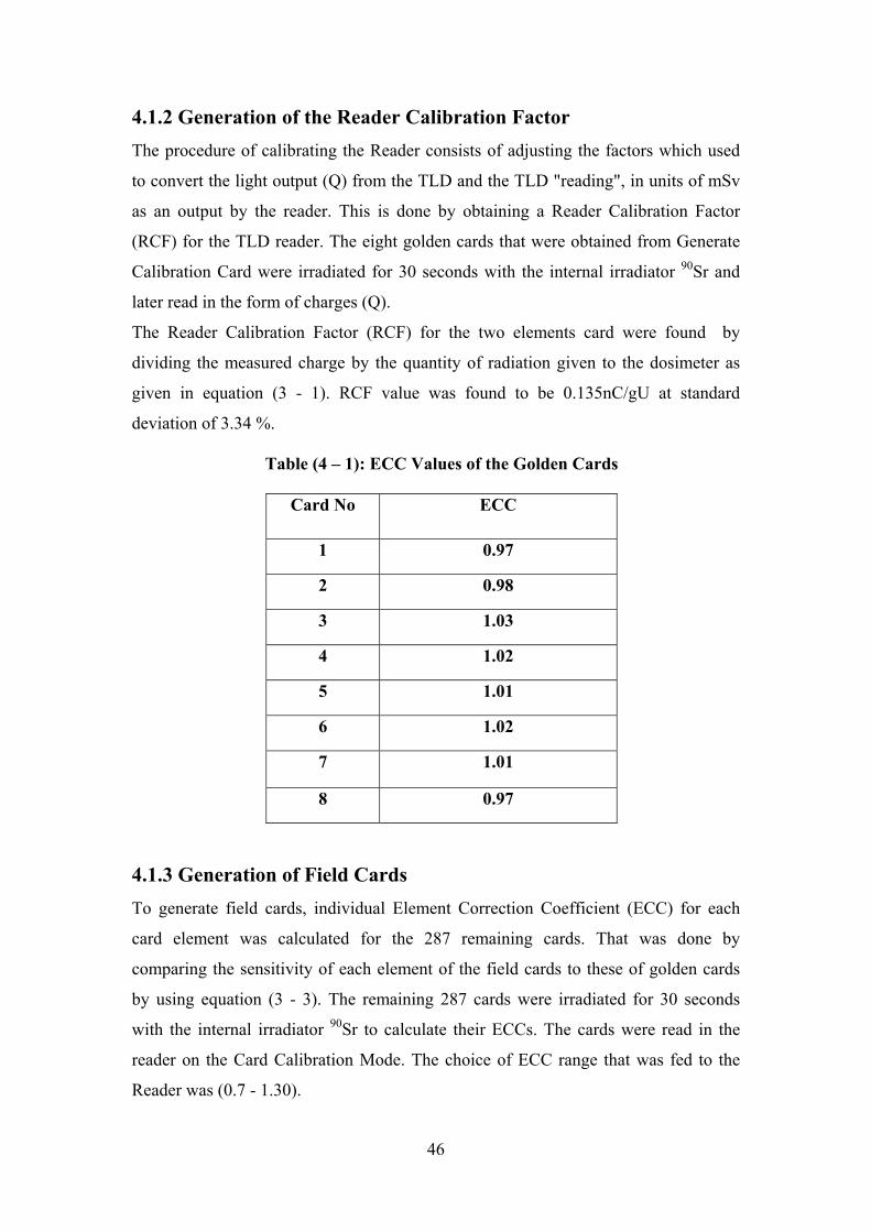
4.1.2 Generation of the Reader Calibration Factor The procedure of calibrating the Reader consists of adjusting the factors which used

to convert the light output (Q) from the TLD and the TLD "reading", in units of mSv

as an output by the reader. This is done by obtaining a Reader Calibration Factor

(RCF) for the TLD reader. The eight golden cards that were obtained from Generate

Calibration Card were irradiated for 30 seconds with the internal irradiator 90Sr and

later read in the form of charges (Q).

The Reader Calibration Factor (RCF) for the two elements card were found by

dividing the measured charge by the quantity of radiation given to the dosimeter as

given in equation (3 - 1). RCF value was found to be 0.135nC/gU at standard

deviation of 3.34 %.

Table (4 – 1): ECC Values of the Golden Cards

Card No ECC

1 0.97

2 0.98

3 1.03

4 1.02

5 1.01

6 1.02

7 1.01

8 0.97

4.1.3 Generation of Field Cards To generate field cards, individual Element Correction Coefficient (ECC) for each

card element was calculated for the 287 remaining cards. That was done by

comparing the sensitivity of each element of the field cards to these of golden cards

by using equation (3 - 3). The remaining 287 cards were irradiated for 30 seconds

with the internal irradiator 90Sr to calculate their ECCs. The cards were read in the

reader on the Card Calibration Mode. The choice of ECC range that was fed to the

Reader was (0.7 - 1.30).

46

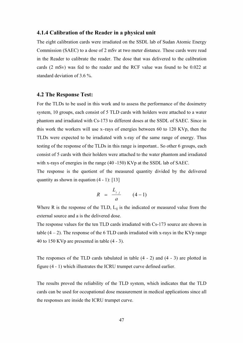
4.1.4 Calibration of the Reader in a physical unit The eight calibration cards were irradiated on the SSDL lab of Sudan Atomic Energy

Commission (SAEC) to a dose of 2 mSv at two meter distance. These cards were read

in the Reader to calibrate the reader. The dose that was delivered to the calibration

cards (2 mSv) was fed to the reader and the RCF value was found to be 0.022 at

standard deviation of 3.6 %.

4.2 The Response Test: For the TLDs to be used in this work and to assess the performance of the dosimetry

system, 10 groups, each consist of 5 TLD cards with holders were attached to a water

phantom and irradiated with Cs-173 to different doses at the SSDL of SAEC. Since in

this work the workers will use x–rays of energies between 60 to 120 KVp, then the

TLDs were expected to be irradiated with x-ray of the same range of energy. Thus

testing of the response of the TLDs in this range is important.. So other 6 groups, each

consist of 5 cards with their holders were attached to the water phantom and irradiated

with x-rays of energies in the range (40 -150) KVp at the SSDL lab of SAEC.

The response is the quotient of the measured quantity divided by the delivered

quantity as shown in equation (4 - 1): [13]

)14( −=a

LR ji

Where R is the response of the TLD, Lij is the indicated or measured value from the

external source and a is the delivered dose.

The response values for the ten TLD cards irradiated with Cs-173 source are shown in

table (4 – 2). The response of the 6 TLD cards irradiated with x-rays in the KVp range

40 to 150 KVp are presented in table (4 - 3).

The responses of the TLD cards tabulated in table (4 - 2) and (4 - 3) are plotted in

figure (4 - 1) which illustrates the ICRU trumpet curve defined earlier.

The results proved the reliability of the TLD system, which indicates that the TLD

cards can be used for occupational dose measurement in medical applications since all

the responses are inside the ICRU trumpet curve.

47

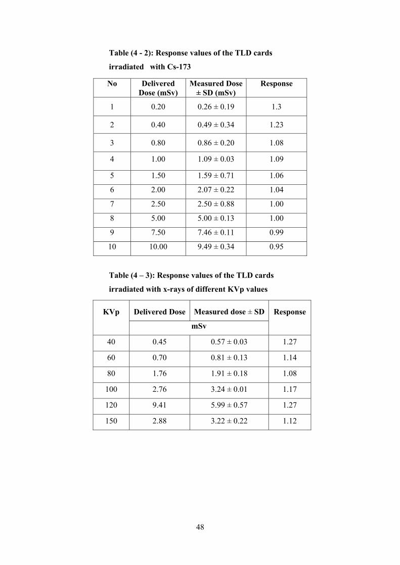
Table (4 - 2): Response values of the TLD cards

irradiated with Cs-173

No Delivered Dose (mSv)

Measured Dose ± SD (mSv)

Response

1 0.20 0.26 ± 0.19 1.3

2 0.40 0.49 ± 0.34 1.23

3 0.80 0.86 ± 0.20 1.08

4 1.00 1.09 ± 0.03 1.09 5 1.50 1.59 ± 0.71 1.06 6 2.00 2.07 ± 0.22 1.04 7 2.50 2.50 ± 0.88 1.00

8

5.00 5.00 ± 0.13 1.00

9

7.50 7.46 ± 0.11 0.99

10

10.00 9.49 ± 0.34 0.95

Table (4 – 3): Response values of the TLD cards

irradiated with x-rays of different KVp values

Measured dose ± SD

Delivered Dose KVp Response

mSv

40 0.45 0.57 ± 0.03 1.27

60 0.81 ± 0.13 0.70 1.14

80 1.76 1.91 ± 0.18 1.08

100 2.76 3.24 ± 0.01 1.17

120 9.41 5.99 ± 0.57 1.27

2.88 3.22 ± 0.22 1.12 150

48

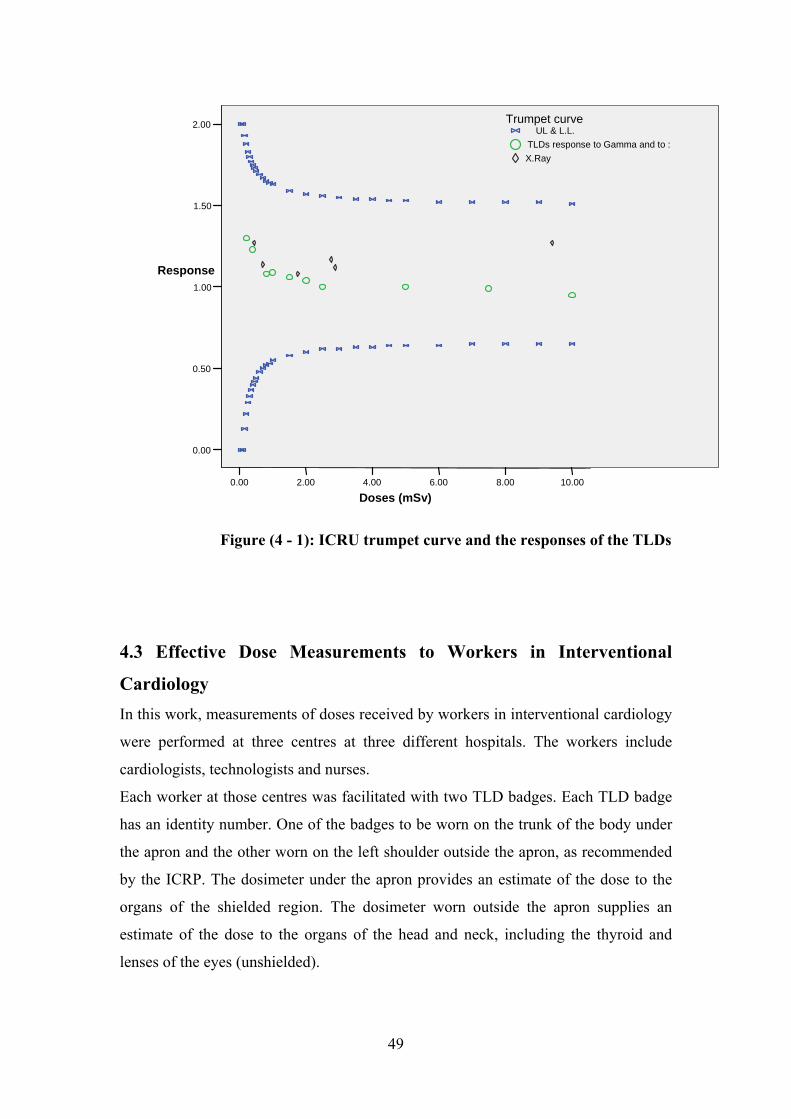
10.008.006.004.002.000.00

Doses (mSv)

2.00

1.50

1.00

0.50

0.00

Response

X.RayTLDs response to Gamma and to :

UL & L.L.Trumpet curve

Figure (4 - 1): ICRU trumpet curve and the responses of the TLDs

4.3 Effective Dose Measurements to Workers in Interventional

Cardiology In this work, measurements of doses received by workers in interventional cardiology

were performed at three centres at three different hospitals. The workers include

cardiologists, technologists and nurses.

Each worker at those centres was facilitated with two TLD badges. Each TLD badge

has an identity number. One of the badges to be worn on the trunk of the body under

the apron and the other worn on the left shoulder outside the apron, as recommended

by the ICRP. The dosimeter under the apron provides an estimate of the dose to the

organs of the shielded region. The dosimeter worn outside the apron supplies an

estimate of the dose to the organs of the head and neck, including the thyroid and

lenses of the eyes (unshielded).

49

A technician at each of the three centres was assigned as radiation protection officer,

to ensure regular and proper use of the TLDs by the workers during their work.

Five control TLD cards for each centre were stored far from exposure to give an

indication to the background during the time of measurement.

After a period of a month the dosimeters were collected. The TLD HARSHAW 6600

Reader was used in the assessment of HP (10).

Cases when the over-apron dosimeters of some workers recorded background dose

values were excluded from the analysis, as this indicated that the personal dosimeters

had not been used.

Results obtained from both dosimeters were used to estimate the occupational

effective dose as recommended by the NCRP Report No 122. Effective dose was

estimated from dosimeter values for HW (under the apron at the waist) and Hn (above

the apron at the neck or the collar level) using equation (2 - 17).

Table (4 – 4) shows the number of the cardiologists, nurses and technologists at each

of the cardiology centres at the three hospitals that is included in this analysis.

Table (4 – 4): Number of cardiologists, nurses and

technologists at the three centres of cardiology

Centre Cardiologists Nurses Technologists

Hospital 1 6 4 1

Hospital 2 4 5 1

Hospital 3 4 4 7

4.3.1. Hospital 1: The number of workers monitored at cardiology department was 15. Three of them

were excluded from the analysis because background dose values were recorded by

their over apron dosimeters.

The background value recorded by the 5 control dosimeters was 0.146 mSv. This

value was subtracted from the readings recorded by the dosimeters over and under the

apron.

50

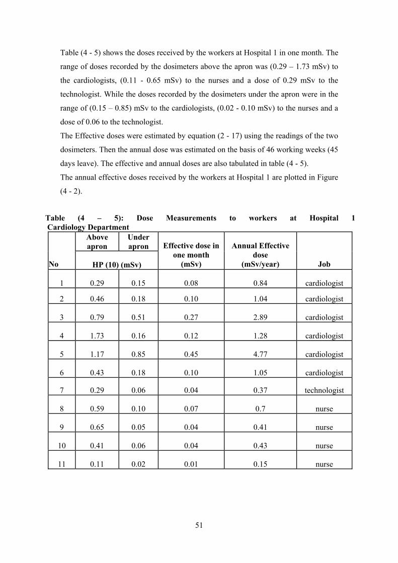
Table (4 - 5) shows the doses received by the workers at Hospital 1 in one month. The

range of doses recorded by the dosimeters above the apron was (0.29 – 1.73 mSv) to

the cardiologists, (0.11 - 0.65 mSv) to the nurses and a dose of 0.29 mSv to the

technologist. While the doses recorded by the dosimeters under the apron were in the

range of (0.15 – 0.85) mSv to the cardiologists, (0.02 - 0.10 mSv) to the nurses and a

dose of 0.06 to the technologist.

The Effective doses were estimated by equation (2 - 17) using the readings of the two

dosimeters. Then the annual dose was estimated on the basis of 46 working weeks (45

days leave). The effective and annual doses are also tabulated in table (4 - 5).

The annual effective doses received by the workers at Hospital 1 are plotted in Figure

(4 - 2).

Table (4 – 5): Dose Measurements to workers at Hospital 1 Cardiology Department

Under apron

Above apron

Job

Annual Effective dose

(mSv/year)

Effective dose in one month

(mSv) HP (10) (mSv) No

cardiologist 1 0.08 0.15 0.29 0.84

0.10 cardiologist 1.04 0.18 0.46 2

cardiologist 2.89 0.27 0.51 0.79 3

cardiologist 1.28 0.12 0.16 1.73 4

cardiologist 4.77 0.45 0.85 1.17 5

cardiologist 1.05 0.10 0.18 0.43 6

technologist 0.37 0.04 0.06 0.29 7

nurse 0.7 0.07 0.10 0.59 8

nurse 0.41 0.04 0.05 0.65 9

nurse 0.43 0.04 0.06 0.41 10

nurse 0.15 0.01 0.02 0.11 11

51

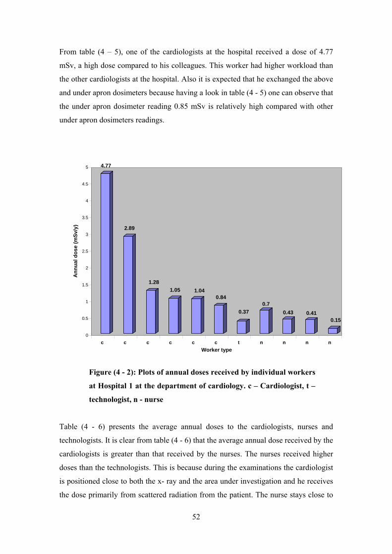
From table (4 – 5), one of the cardiologists at the hospital received a dose of 4.77

mSv, a high dose compared to his colleagues. This worker had higher workload than

the other cardiologists at the hospital. Also it is expected that he exchanged the above

and under apron dosimeters because having a look in table (4 - 5) one can observe that

the under apron dosimeter reading 0.85 mSv is relatively high compared with other

under apron dosimeters readings.

4.77

2.89

1.281.05 1.04

0.84

0.370.7

0.43 0.410.15

0

0.5

1

1.5

2

2.5

3

3.5

4

4.5

5

Ann

ual d

ose

(mSv

/y)

c c c c c c t n n n n Worker type

Figure (4 - 2): Plots of annual doses received by individual workers

at Hospital 1 at the department of cardiology. c – Cardiologist, t –

technologist, n - nurse

Table (4 - 6) presents the average annual doses to the cardiologists, nurses and

technologists. It is clear from table (4 - 6) that the average annual dose received by the

cardiologists is greater than that received by the nurses. The nurses received higher

doses than the technologists. This is because during the examinations the cardiologist

is positioned close to both the x- ray and the area under investigation and he receives

the dose primarily from scattered radiation from the patient. The nurse stays close to

52

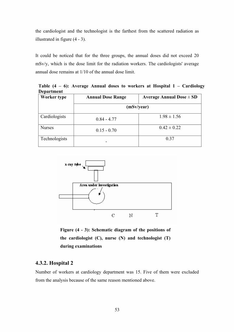
the cardiologist and the technologist is the farthest from the scattered radiation as

illustrated in figure (4 - 3).

It could be noticed that for the three groups, the annual doses did not exceed 20

mSv/y, which is the dose limit for the radiation workers. The cardiologists' average

annual dose remains at 1/10 of the annual dose limit.

Figure (4 - 3): Schematic diagram of the positions of

the cardiologist (C), nurse (N) and technologist (T)

during examinations

Table (4 – 6): Average Annual doses to workers at Hospital 1 – Cardiology Department

Average Annual Dose ± SD

4.3.2. Hospital 2 Number of workers at cardiology department was 15. Five of them were excluded

from the analysis because of the same reason mentioned above.

Annual Dose Range Worker type

(mSv/year)

Cardiologists 0.84 - 4.77 1.98 ± 1.56

Nurses 0.15 - 0.70 0.42 ± 0.22

Technologists 0.37 -

53

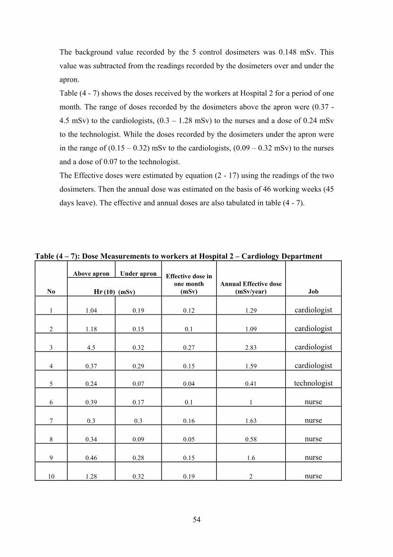
The background value recorded by the 5 control dosimeters was 0.148 mSv. This

value was subtracted from the readings recorded by the dosimeters over and under the

apron.

Table (4 - 7) shows the doses received by the workers at Hospital 2 for a period of one

month. The range of doses recorded by the dosimeters above the apron were (0.37 -

4.5 mSv) to the cardiologists, (0.3 – 1.28 mSv) to the nurses and a dose of 0.24 mSv

to the technologist. While the doses recorded by the dosimeters under the apron were

in the range of (0.15 – 0.32) mSv to the cardiologists, (0.09 – 0.32 mSv) to the nurses

and a dose of 0.07 to the technologist.

The Effective doses were estimated by equation (2 - 17) using the readings of the two

dosimeters. Then the annual dose was estimated on the basis of 46 working weeks (45

days leave). The effective and annual doses are also tabulated in table (4 - 7).

Table (4 – 7): Dose Measurements to workers at Hospital 2 – Cardiology Department

Under apron Above apron

Job Annual Effective dose

(mSv/year)

Effective dose in one month

(mSv) HP (10) (mSv) No

cardiologist 1.29 0.12 0.19 1.04 1

cardiologist 1.09 0.1 0.15 1.18 2

cardiologist 2.83 0.27 0.32 4.5 3

cardiologist 1.59 0.15 0.29 0.37 4

technologist 0.41 0.04 0.07 0.24 5

nurse 1 0.1 0.17 0.39 6

nurse 1.63 0.16 0.3 0.3 7

nurse 0.58 0.05 0.09 0.34 8

nurse 1.6 0.15 0.28 0.46 9

nurse 2 0.19 0.32 1.28 10

54

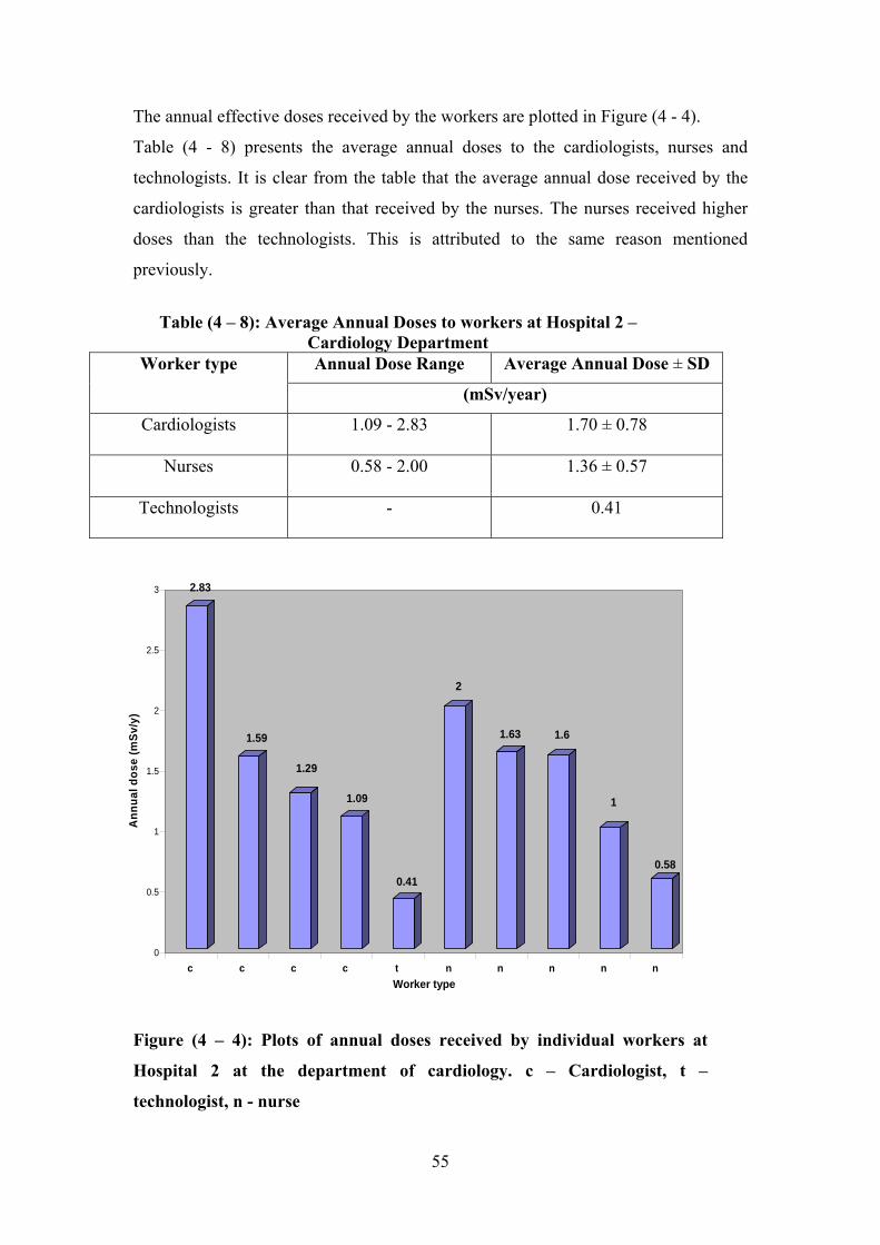
The annual effective doses received by the workers are plotted in Figure (4 - 4).

Table (4 - 8) presents the average annual doses to the cardiologists, nurses and

technologists. It is clear from the table that the average annual dose received by the

cardiologists is greater than that received by the nurses. The nurses received higher

doses than the technologists. This is attributed to the same reason mentioned

previously.

Table (4 – 8): Average Annual Doses to workers at Hospital 2 – Cardiology Department Annual Dose Range Average Annual Dose ± SD Worker type

(mSv/year)

Cardiologists 1.09 - 2.83 1.70 ± 0.78

Nurses 0.58 - 2.00 1.36 ± 0.57

Technologists - 0.41

2.83

1.59

1.29

1.09

0.41

2

1.63 1.6

1

0.58

0

0.5

1

1.5

2

2.5

3

Ann

ual d

ose

(mSv

/y)

c c c c t n n n n n Worker type

Figure (4 – 4): Plots of annual doses received by individual workers at

Hospital 2 at the department of cardiology. c – Cardiologist, t –

technologist, n - nurse

55

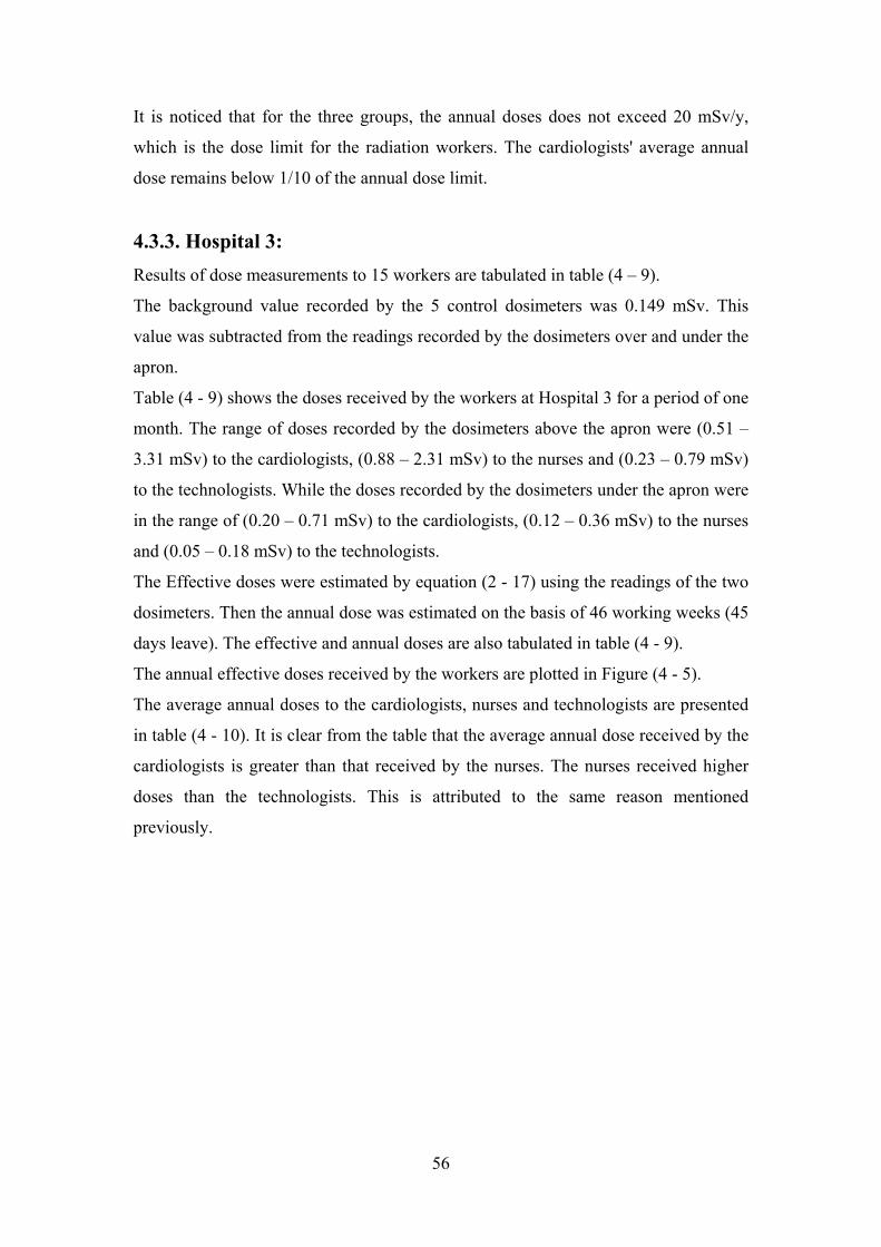
It is noticed that for the three groups, the annual doses does not exceed 20 mSv/y,

which is the dose limit for the radiation workers. The cardiologists' average annual

dose remains below 1/10 of the annual dose limit.

4.3.3. Hospital 3: Results of dose measurements to 15 workers are tabulated in table (4 – 9).

The background value recorded by the 5 control dosimeters was 0.149 mSv. This

value was subtracted from the readings recorded by the dosimeters over and under the

apron.

Table (4 - 9) shows the doses received by the workers at Hospital 3 for a period of one

month. The range of doses recorded by the dosimeters above the apron were (0.51 –

3.31 mSv) to the cardiologists, (0.88 – 2.31 mSv) to the nurses and (0.23 – 0.79 mSv)

to the technologists. While the doses recorded by the dosimeters under the apron were

in the range of (0.20 – 0.71 mSv) to the cardiologists, (0.12 – 0.36 mSv) to the nurses

and (0.05 – 0.18 mSv) to the technologists.

The Effective doses were estimated by equation (2 - 17) using the readings of the two

dosimeters. Then the annual dose was estimated on the basis of 46 working weeks (45

days leave). The effective and annual doses are also tabulated in table (4 - 9).

The annual effective doses received by the workers are plotted in Figure (4 - 5).

The average annual doses to the cardiologists, nurses and technologists are presented

in table (4 - 10). It is clear from the table that the average annual dose received by the

cardiologists is greater than that received by the nurses. The nurses received higher

doses than the technologists. This is attributed to the same reason mentioned

previously.

56

Table (4 – 9): Dose Measurements to workers at Hospital 3 – Cardiology Department

Under apron

Above apron

Job

Annual Effective dose

(mSv/y)

Effective dose in one month

(mSv) HP (10) (mSv) No

cardiologist 2.07 0.2 0.23 3.31 1

2 cardiologist 4.4 0.42 0.71 2.53

3 0.22 1.92 0.16 cardiologist 1.67

0.11 cardiologist 1.17 0.2 0.51 4

technologist 0.33 0.03 0.23 5 0.05

technologist 0.68 0.06 0.12 0.24 6

technologist 0.46 0.04 0.06 0.56 7

0.53 technologist 1.1 0.11 0.18 8

technologist 0.32 0.03 9 0.26 0.05

0.12 technologist 0.75 0.07 0.41 10

technologist 0.93 11 0.14 0.79 0.09

12 0.88 0.09 0.13 0.9 nurse

0.36 2.08 0.2 nurse 0.84 13

nurse 1.23 14 0.12 2.31 0.12

1.32 0.17 0.27 1.75 nurse 15

57

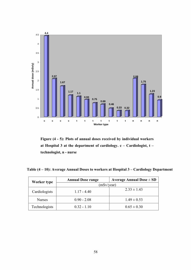
Figure (4 - 5): Plots of annual doses received by individual workers

at Hospital 3 at the department of cardiology. c – Cardiologist, t –

technologist, n - nurse

Table (4 – 10): Average Annual Doses to workers at Hospital 3 – Cardiology Department

Annual Dose range Average Annual Dose ± SD Worker type (mSv/year)

Cardiologists 1.17 - 4.40 2.33 ± 1.43

Nurses 0.90 - 2.08 1.49 ± 0.53

Technologists 0.32 - 1.10 0.65 ± 0.30

4.4

2.07

1.67

1.17 1.10.93

0.750.68

0.460.33 0.32

2.08

1.75

1.23

0.9

0

0.5

1

1.5

2

2.5

3

3.5

4

4.5A

nnua

l dos

e (m

Sv/y

)

c c c c t t t t t t t n n n n Worker type

58

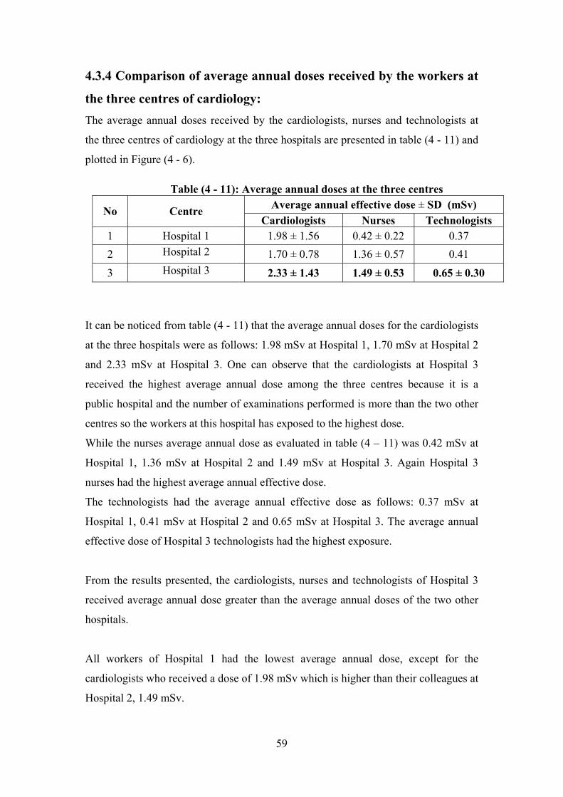
4.3.4 Comparison of average annual doses received by the workers at

the three centres of cardiology: The average annual doses received by the cardiologists, nurses and technologists at

the three centres of cardiology at the three hospitals are presented in table (4 - 11) and

plotted in Figure (4 - 6).

It can be noticed from table (4 - 11) that the average annual doses for the cardiologists

at the three hospitals were as follows: 1.98 mSv at Hospital 1, 1.70 mSv at Hospital 2

and 2.33 mSv at Hospital 3. One can observe that the cardiologists at Hospital 3

received the highest average annual dose among the three centres because it is a

public hospital and the number of examinations performed is more than the two other

centres so the workers at this hospital has exposed to the highest dose.

While the nurses average annual dose as evaluated in table (4 – 11) was 0.42 mSv at

Hospital 1, 1.36 mSv at Hospital 2 and 1.49 mSv at Hospital 3. Again Hospital 3

nurses had the highest average annual effective dose.

Table (4 - 11): Average annual doses at the three centres Average annual effective dose ± SD (mSv) No Centre

Cardiologists Nurses Technologists 1 Hospital 1 1.98 ± 1.56 0.42 ± 0.22 0.37

Hospital 2 2 1.70 ± 0.78 1.36 ± 0.57 0.41 Hospital 3 2.33 ± 1.43 1.49 ± 0.53 0.65 ± 0.30 3

The technologists had the average annual effective dose as follows: 0.37 mSv at

Hospital 1, 0.41 mSv at Hospital 2 and 0.65 mSv at Hospital 3. The average annual

effective dose of Hospital 3 technologists had the highest exposure.

From the results presented, the cardiologists, nurses and technologists of Hospital 3

received average annual dose greater than the average annual doses of the two other

hospitals.

All workers of Hospital 1 had the lowest average annual dose, except for the

cardiologists who received a dose of 1.98 mSv which is higher than their colleagues at

Hospital 2, 1.49 mSv.

59

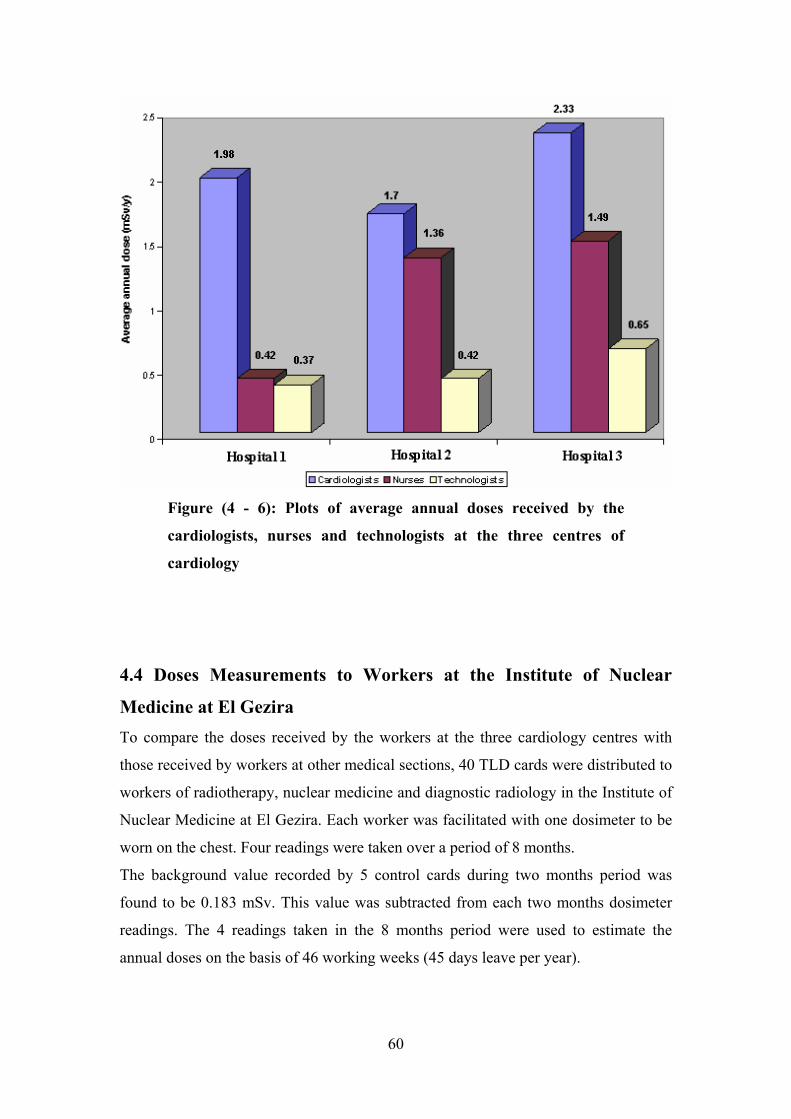
Figure (4 - 6): Plots of average annual doses received by the

cardiologists, nurses and technologists at the three centres of

cardiology

4.4 Doses Measurements to Workers at the Institute of Nuclear

Medicine at El Gezira To compare the doses received by the workers at the three cardiology centres with

those received by workers at other medical sections, 40 TLD cards were distributed to

workers of radiotherapy, nuclear medicine and diagnostic radiology in the Institute of

Nuclear Medicine at El Gezira. Each worker was facilitated with one dosimeter to be

worn on the chest. Four readings were taken over a period of 8 months.

The background value recorded by 5 control cards during two months period was

found to be 0.183 mSv. This value was subtracted from each two months dosimeter

readings. The 4 readings taken in the 8 months period were used to estimate the

annual doses on the basis of 46 working weeks (45 days leave per year).

60

The annual doses received by workers at each of the three medical practices,

radiotherapy, nuclear medicine and diagnostic radiology are presented in tables (4 -

12), (4 - 13) & (4 - 14) and plotted in figures (4 - 7), (4 - 8) & (4 - 9) respectively.

Table (4 - 12): Annual doses of radiotherapy section

workers

Job AnnualDose

(mSv/y) No

doctor 0.51 1

doctor 0.3 2

doctor 0.15 3

technologist 0.21 4

technologist 0.21 5

0.31 technologist 6

0.22 technologist 7

0.04 technologist 8

0.48 technologist 9

0.65 nurse 10

61

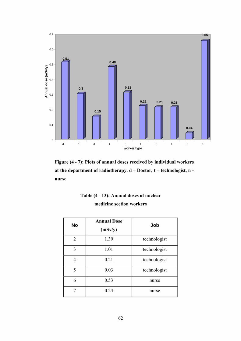
0.51

0.3

0.15

0.48

0.31

0.22 0.21 0.21

0.04

0.65

0

0.1

0.2

0.3

0.4

0.5

0.6

0.7

Ann

ual d

ose

(mSv

/y)

d d d t t t t t t nworker type

Figure (4 - 7): Plots of annual doses received by individual workers

at the department of radiotherapy. d – Doctor, t – technologist, n -

nurse

Table (4 - 13): Annual doses of nuclear

medicine section workers

Annual Dose No Job

(mSv/y)

1.39 technologist 2

1.01 technologist 3

0.21 technologist 4

0.03 technologist 5

0.53 nurse 6

0.24 nurse 7

62

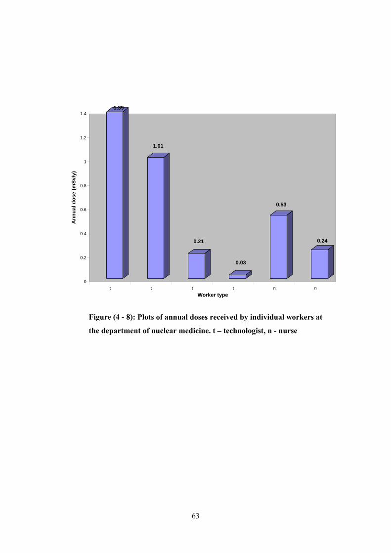
1.39

1.01

0.21

0.03

0.53

0.24

0

0.2

0.4

0.6

0.8

1

1.2

1.4

Ann

ual d

ose

(mSv

/y)

t t t t n nWorker type

Figure (4 - 8): Plots of annual doses received by individual workers at

the department of nuclear medicine. t – technologist, n - nurse

63

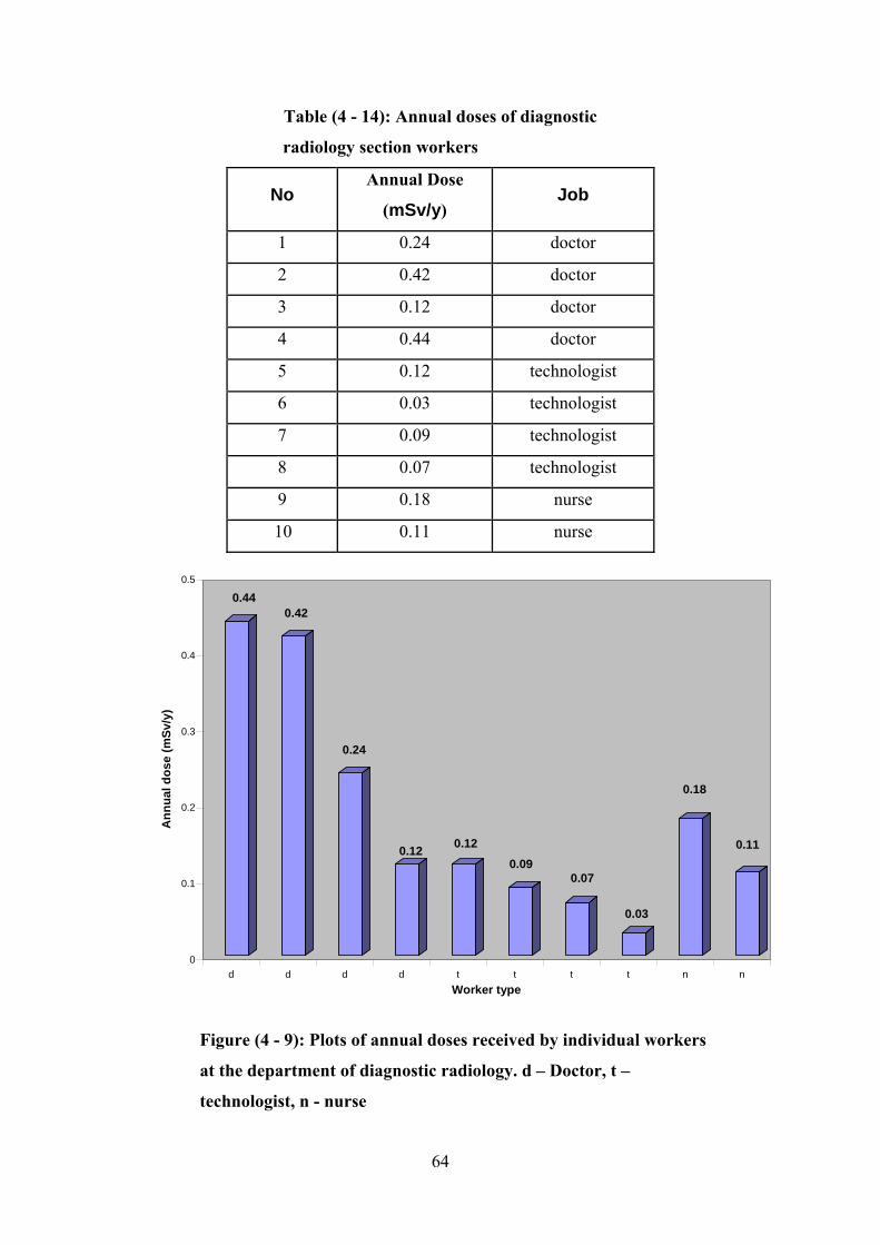
Table (4 - 14): Annual doses of diagnostic

radiology section workers

Annual Dose No Job

(mSv/y)

0.24 doctor 1

0.42 doctor 2

0.12 doctor 3

0.44 doctor 4

0.12 technologist 5

0.03 technologist 6

0.09 technologist 7

0.07 technologist 8

0.18 nurse 9

10 0.11 nurse

0.440.42

0.24

0.12 0.120.09

0.07

0.03

0.18

0.11

0

0.1

0.2

0.3

0.4

0.5

Ann

ual d

ose

(mSv

/y)

d d d d t t t t n nWorker type

Figure (4 - 9): Plots of annual doses received by individual workers

at the department of diagnostic radiology. d – Doctor, t –

technologist, n - nurse

64

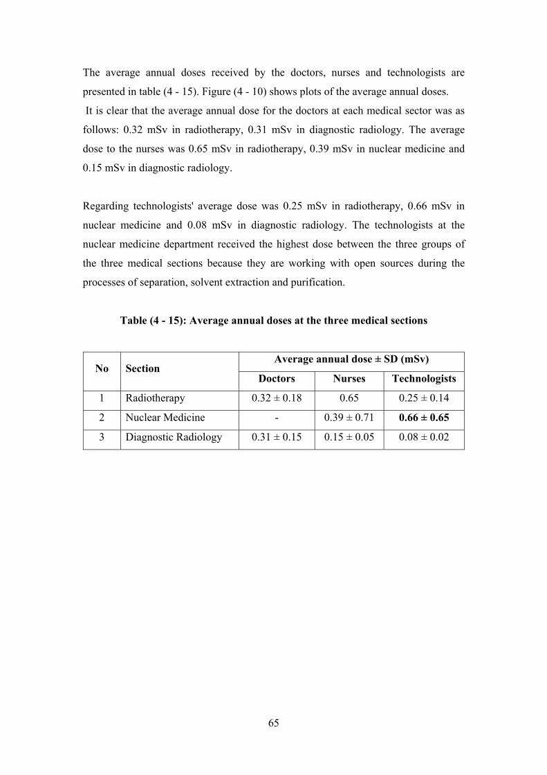
The average annual doses received by the doctors, nurses and technologists are

presented in table (4 - 15). Figure (4 - 10) shows plots of the average annual doses.

It is clear that the average annual dose for the doctors at each medical sector was as

follows: 0.32 mSv in radiotherapy, 0.31 mSv in diagnostic radiology. The average

dose to the nurses was 0.65 mSv in radiotherapy, 0.39 mSv in nuclear medicine and

0.15 mSv in diagnostic radiology.

Regarding technologists' average dose was 0.25 mSv in radiotherapy, 0.66 mSv in

nuclear medicine and 0.08 mSv in diagnostic radiology. The technologists at the

nuclear medicine department received the highest dose between the three groups of

the three medical sections because they are working with open sources during the

processes of separation, solvent extraction and purification.

Table (4 - 15): Average annual doses at the three medical sections

Average annual dose ± SD (mSv) No Section

Doctors Nurses Technologists

1 Radiotherapy 0.32 ± 0.18 0.65 0.25 ± 0.14

0.66 ± 0.65 2 Nuclear Medicine - 0.39 ± 0.71

3 Diagnostic Radiology 0.31 ± 0.15 0.15 ± 0.05 0.08 ± 0.02

65

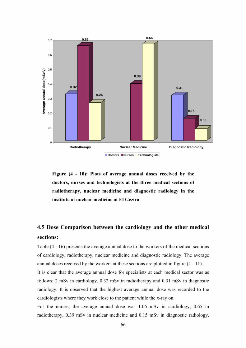
0.32

0.65

0.26

0.39

0.66

0.31

0.15

0.08

0

0.1

0.2

0.3

0.4

0.5

0.6

0.7A

vera

ge a

nnua

l dos

e(m

Sv/y

)

Radiotherapy Nuclear Medicine Diagnostic Radiology

Doctors Nurses Technologists

Figure (4 - 10): Plots of average annual doses received by the

doctors, nurses and technologists at the three medical sections of

radiotherapy, nuclear medicine and diagnostic radiology in the

institute of nuclear medicine at El Gezira

4.5 Dose Comparison between the cardiology and the other medical

sections: Table (4 - 16) presents the average annual dose to the workers of the medical sections

of cardiology, radiotherapy, nuclear medicine and diagnostic radiology. The average

annual doses received by the workers at these sections are plotted in figure (4 - 11).

It is clear that the average annual dose for specialists at each medical sector was as

follows: 2 mSv in cardiology, 0.32 mSv in radiotherapy and 0.31 mSv in diagnostic

radiology. It is observed that the highest average annual dose was recorded to the

cardiologists where they work close to the patient while the x-ray on.

For the nurses, the average annual dose was 1.06 mSv in cardiology, 0.65 in

radiotherapy, 0.39 mSv in nuclear medicine and 0.15 mSv in diagnostic radiology.

66

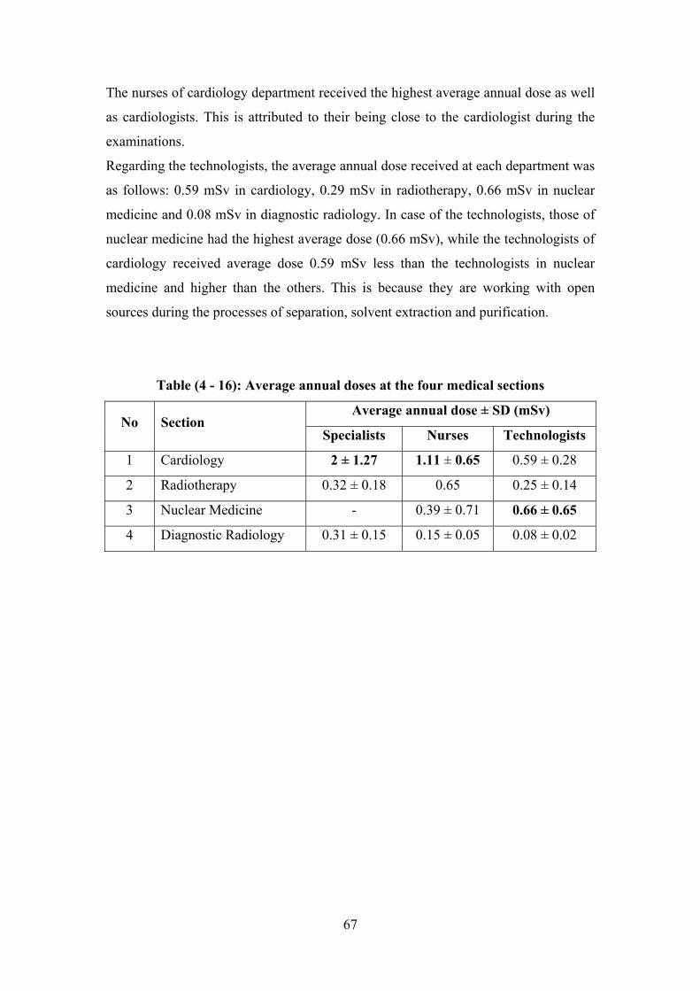
The nurses of cardiology department received the highest average annual dose as well

as cardiologists. This is attributed to their being close to the cardiologist during the

examinations.

Regarding the technologists, the average annual dose received at each department was

as follows: 0.59 mSv in cardiology, 0.29 mSv in radiotherapy, 0.66 mSv in nuclear

medicine and 0.08 mSv in diagnostic radiology. In case of the technologists, those of

nuclear medicine had the highest average dose (0.66 mSv), while the technologists of

cardiology received average dose 0.59 mSv less than the technologists in nuclear

medicine and higher than the others. This is because they are working with open

sources during the processes of separation, solvent extraction and purification.

Table (4 - 16): Average annual doses at the four medical sections

Average annual dose ± SD (mSv) No Section

Specialists Nurses Technologists

1.11 ± 0.65 2 ± 1.27 1 Cardiology 0.59 ± 0.28

2 Radiotherapy 0.32 ± 0.18 0.65 0.25 ± 0.14

0.66 ± 0.65 3 Nuclear Medicine - 0.39 ± 0.71

4 Diagnostic Radiology 0.31 ± 0.15 0.15 ± 0.05 0.08 ± 0.02

67

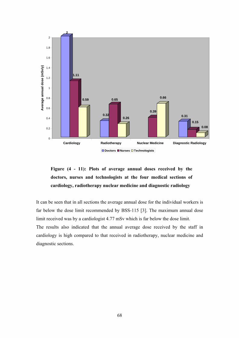
2

1.11

0.59

0.32

0.65

0.26

0.39

0.66

0.31

0.150.08

0

0.2

0.4

0.6

0.8

1

1.2

1.4

1.6

1.8

2

Ave

rage

ann

ual d

ose

(mSv

/y)

Cardiology Radiotherapy Nuclear Medicine Diagnostic Radiology

Doctors Nurses Technologists

Figure (4 - 11): Plots of average annual doses received by the

doctors, nurses and technologists at the four medical sections of

cardiology, radiotherapy nuclear medicine and diagnostic radiology

It can be seen that in all sections the average annual dose for the individual workers is

far below the dose limit recommended by BSS-115 [3]. The maximum annual dose

limit received was by a cardiologist 4.77 mSv which is far below the dose limit.

The results also indicated that the annual average dose received by the staff in

cardiology is high compared to that received in radiotherapy, nuclear medicine and

diagnostic sections.

68

Chapter 5

Conclusion and Recommendations

The study overviews the status of occupational exposure for workers of interventional

cardiology in Sudan.

Personal doses measured during this survey generally not exceed the dose limits

specified in the BSS-115 [3]. Doses to interventional cardiology staff, in particular

cardiologists, were found to be relatively high.

Staff doses from interventional cardiology can be quite high. It is important that these

potentially high radiation doses are minimized. Many variables can affect staff

exposure: distance, direction, use of protective screens, procedure, skill, training,

equipment performance, etc.

On the other hand, this study shows the need to set constant individual monitoring for

the workers to assist in reducing the occupational exposure.

69

References:

1. http://en.wikipedia.org/wiki/interventional cardiology

2. United Nations Scientific Committee on the Effects of Atomic Radiation.

Sources and Effects of Ionizing Radiation. UNSCEAR 2000 report to the

General Assembly with scientific annexes. Annex E. Occupational radiation

exposures. (Available at www. Unscear.org). New York: United Nations.

2000.

3. International Basic Safety Standards for protection against ionizing radiation

and for the safety of radiation sources, safety series No. 115, IAEA, Vienna.

1996, pp. 91 .96.

4. NCRP Report No. 122. Use of Personal Monitors to Estimate Effective Dose

Equivalent and Effective Dose to Workers for External Exposure to Low-LET

Radiation. Copyright © National Council on Radiation Protection and

Measurements.1995.

5. Azza Abdalrahim. Thesis in Fulfillment of M.Sc. Degree. Khartoum

University, Physics Department. Measurements of doses to patients in

diagnostic Radiology Using TLDs. 2001.

6. William R. Hendee and E. Russell Ritenour. Medical Imaging Physics. 4th

Edition. Wiley & Sons, INC., publication. U.S.A. Copyright © by Wiley-Liss,

INC., New York. 2002.

7. E.B. Padgorsak. Radiation oncology physics. Technical editor- IAEA. Vienna.

ISBN 92-0-107304-6. 2005.

8. Ibrahim Shadad. Thesis in Fulfillment of M.Sc. Degree. Khartoum University,

Physics Department. Determination of Nitrogen in Food Stuffs using 14 –

MeV Neutrons. 1988.

9. Occupational Radiation Protection; Safety Guide/ Jointly Sponsored by the

International Atomic Energy Agency and the International Labour Office.

Vienna: The International Atomic Energy Agency, 1999.

10. E Vano. Radiation Exposure to cardiologists: How it could be reduced. BMJ

Publishing Group & British cardiac Society, 2002. Accessed in Google

70

11. Practical Radiation Technical Manual – Individual Monitoring. IAEA, Viena,

2004.

12. K Faulkner, NW Marshal and DJ Rawlings. Optimization of Staff Protection.

Regional Medical Physics Department. Newcastle General Hospital.

13. Operator's Manual. Model 6600 Automated TLD Reader with WinREMS.

Publication No. 6600W-O0602-005. U.S.A. Copyright © Saint-Gobain

Ceramics & Plastics, INC. 2002

14. Riener Esser. ICRU Trumpet Curve. Thermo Fisher Scientific, HARSHAW

Dosimetry Solutions.

71