Embed Size (px)
Citation preview
ROBUST MOBILE ROBOT LOCALIZATION:
FROM SINGLE-ROBOT UNCERTAINTIES
TO MULTI-ROBOT INTERDEPENDENCIES
by
Stergios I. Roumeliotis
A Dissertation Presented to the
FACULTY OF THE GRADUATE SCHOOL
UNIVERSITY OF SOUTHERN CALIFORNIA
In Partial Fulllment of the
Requirements for the Degree
DOCTOR OF PHILOSOPHY
(Electrical Engineering)
May 2000
Copyright 2000 Stergios I. Roumeliotis

i

Dedication
This dissertation is dedicated to my parents, all three of them.
ii
Acknowledgments
I thank my advisor, Professor Bekey for trusting me these last 5 years with
extremely challenging projects and for being a wonderful source of scientic
insight. Working closely with him all these years has given me the opportu-
nity to observe a unique personality who has helped to shape and in uence
various scientic elds for the past 50 years. I will also never forget the en-
couraging words of his wonderful wife, Dr. Shirley Bekey only a few days
before my defense. I will always be grateful to the both of you.
I would also like to thank the members of my committee, Professors Elias
Kosmatopoulos, Jerry Mendel, Stefan Schaal and Gaurav Sukhatme for their
contribution during the preparation of this dissertation. Special thanks go to
Drs. Guillermo Rodriguez, Dave Bayard, and Richard Volpe at JPL, NASA
for their assistance while working on the Mars rover localization project.
During my years of graduate school I was very lucky to meet and inter-
act with Professors Ralph Etienne-Cummings, Petros Ioannou, Bart Kosko,
Chris Kyriakakis, Kostas Kyriakopoulos, Nikos Papanikolopoulos, George
Saridis and Kimon Valavanis.
During my last ve years in the robotics lab I met many wonderful people.
I would like to thank Professor Maja Mataric for listening and helping me to
shape and form new ideas as I am preparing for my postgraduate research.
I also owe her much gratitude for her constant support during extremely
dicult moments. My good friend Mike McHenry for believing in me and
iii

giving me endless encouragement. Our lengthy conversations helped me un-
derstand and appreciate American culture. While we may have had diering
viewpoints, I would like to think that we both became better acquainted
with one another's culture. Through these conversations, my love and ap-
preciation for the cradle of civilization, Greece, has become even stronger.
Jim Montgomery for making me very cautious of what I eat and breathe.
Ayanna Howard for being such a pleasant and warm oce-mate. Kale Har-
bick and Steve Goldberg for helping me to deal with \evil" hardware and
software. Monica Nicolesku for always smiling even under extreme condi-
tions. Brian Gerkey, Chad Jenkins, Nitin Mohan, Aswath Mohan, and Ste-
fan Weber for their fun-loving company. Dani Goldberg and Barry Werger
for being such \gutte neshomes"! Javi Mesa-Martinez, Maite Lopez-Sanchez,
and Raul Suarez for bringing a Latin/Mediterranean air in the lab. Kusum
Shori for being like a mother to all of us. Her warm smile helped brighten
even the darkest days. Paolo Pirjanian for being such a bright collaborator
and a wonderful friend. Those who know him also know of his amazing story
of courage and bravery similar to the ones of hundreds of thousands of per-
secuted Armenians throughout this century. God blessed him and his wife,
Hrachik for their struggles with a beautiful bundle of joy named Andre.
While staying in the states I made new friends that kept fresh the spirit
of my homeland. Kostas Koutsikos, Dimitris Kostakis and Argyris Argy-
rou were the rst greek friends I made in this country. The last few years
this city became quite livable with the company some new friends: Thanasi
\fenomeno" Mouchtari, Mano Lalioti, Andrea Dandali, Panagioti Georgiou,
Persefoni Kechagia, Panagiota Poirazi and Ariadni Liokati. Amongst them
Elias, half-brother half-friend, who shared with us endless stories from his
own \country", Kozani.
Before coming to USC, I spent probably the best years of my life amongst
iv
some of the brightest and warm people. Studying many long hours with
Dimitri Oikonomou made my college years a breeze. I learned from him that
people you work with can also become your best friends. Theodoris Papa-
georgiou brought an adventurous spin in my life and showed me how to keep
my strength during the most dicult times. I thank him for reading with pa-
tience hundreds of e-mails during the last ve years and being a caring friend.
Giorgos Tzou as for challenging me with long conversations always having
the opposite opinion. Spyros Raptis for helping me out so many times. Chris-
tos Malliopoulos for being the embodiment of fun. Elias Kalantzis, Stefanos
Kantartzis, Aggelos Liveris, and Fotini Simistira for bringing their warmth
into this group. Telis Georgiou for being so patient with all our craziness.
Outside NTUA there are three more people that were always very close to
me. Giorgos Dionisiou, Nikos Ntamparakis and Giannis Velentzas. Thank
you for being there for me.
Life is so beautiful when you are around great friends but it has more
meaning when you share it with a soul mate. Joanna Giforos came in my
life three years ago and brought a golden heart with her. Without her smile
and kindness I would not be writing these lines now.
Finally, my gratitude goes to my family. My sister Gioula and my brother
Marios have been there for me during some of the most dicult times of my
life. My parents Giannis and Stavroula devoted every moment of their life to
us. My grandmother Maria helped nurture us like a second mother. Their
innite love and caring helped us nd our way in life. I do not think there
are enough words to describe how much I thank them.
v
Contents
Dedication ii
Acknowledgments iii
List Of Figures x
Abstract xviii
1 Introduction and Problem Statement 1
1.1 Motivation . . . . . . . . . . . . . . . . . . . . . . . . . . . . . 1
1.2 Assumptions made in this Thesis . . . . . . . . . . . . . . . . 3
1.3 Problem Statement . . . . . . . . . . . . . . . . . . . . . . . . 3
2 Literature Review 7
2.1 Position Tracking . . . . . . . . . . . . . . . . . . . . . . . . . 7
2.1.1 Position Tracking and Kalman ltering . . . . . . . . . 8
2.1.2 Position Tracking and Landmarks . . . . . . . . . . . . 9
2.2 Absolute Localization . . . . . . . . . . . . . . . . . . . . . . . 12
2.2.1 Absolute Localization and Landmarks . . . . . . . . . 12
2.2.2 Absolute Localization and Dense Sensor Maps . . . . . 15
2.3 Rule Based Sensor Fusion . . . . . . . . . . . . . . . . . . . . 17
2.4 Multiple Hypothesis Testing . . . . . . . . . . . . . . . . . . . 18
2.4.1 Previous Approaches . . . . . . . . . . . . . . . . . . . 18
2.4.2 Proposed Extensions to Mobile Robot Localization . . 19
vi
3 Bayesian Estimation and Kalman Filtering: Multiple Hy-
pothesis Tracking 22
3.1 Introduction . . . . . . . . . . . . . . . . . . . . . . . . . . . . 22
3.2 The Multiple Hypotheses Tracking Approach . . . . . . . . . . 27
3.2.1 Absolute Localization: The \kidnapped robot" Prob-
lem, Position Tracking, and Landmark Detection . . . 28
3.2.1.1 Perfect Landmark Recognition, ImperfectOdom-
etry . . . . . . . . . . . . . . . . . . . . . . . 32
3.2.1.2 Imperfect Landmark Recognition, Imperfect
Odometry . . . . . . . . . . . . . . . . . . . . 35
3.2.2 Simulation Results . . . . . . . . . . . . . . . . . . . . 42
3.2.3 Environments with many types of features . . . . . . . 46
3.2.4 Experimental Results . . . . . . . . . . . . . . . . . . . 48
3.2.5 Extensions . . . . . . . . . . . . . . . . . . . . . . . . . 66
4 Smoother Based Attitude Estimation 2-D 77
4.1 Introduction . . . . . . . . . . . . . . . . . . . . . . . . . . . . 77
4.1.1 Localization and Attitude estimation . . . . . . . . . . 78
4.1.1.1 Attitude Measuring Devices . . . . . . . . . . 79
4.1.1.2 Dynamic Model Replacement . . . . . . . . . 81
4.1.2 Forms of the Kalman lter . . . . . . . . . . . . . . . . 83
4.1.2.1 Indirect versus Direct Kalman lter . . . . . . 84
4.1.2.2 Feedforward versus feedback Indirect Kalman
lter . . . . . . . . . . . . . . . . . . . . . . . 86
4.1.3 Planar Motion: One Gyro Case - Bias Compensation . 86
4.1.3.1 Systron Donner Quartz Gyro . . . . . . . . . 87
4.1.3.2 Gyro Noise Model . . . . . . . . . . . . . . . 88
4.1.3.3 Equations of the feedback Indirect Kalman
lter . . . . . . . . . . . . . . . . . . . . . . . 89
4.1.3.4 Observability . . . . . . . . . . . . . . . . . . 96
4.1.3.5 Backward lter . . . . . . . . . . . . . . . . . 99
4.1.3.6 Smoother . . . . . . . . . . . . . . . . . . . . 101
5 Smoother Based Attitude Estimation 3-D 113
5.1 Introduction . . . . . . . . . . . . . . . . . . . . . . . . . . . . 113
5.1.1 Quaternions in Attitude Representation . . . . . . . . 117
5.1.2 Attitude kinematics . . . . . . . . . . . . . . . . . . . . 118
vii
5.1.3 Discrete system: Indirect forward Kalman lter equa-
tions . . . . . . . . . . . . . . . . . . . . . . . . . . . . 123
5.1.3.1 Propagation . . . . . . . . . . . . . . . . . . . 123
5.1.3.2 Update . . . . . . . . . . . . . . . . . . . . . 125
5.1.3.3 Observation model . . . . . . . . . . . . . . . 126
5.1.4 Backward lter . . . . . . . . . . . . . . . . . . . . . . 128
5.1.5 Smoother . . . . . . . . . . . . . . . . . . . . . . . . . 130
5.2 From Attitude Estimates to Position Estimates . . . . . . . . 136
5.3 Conclusions . . . . . . . . . . . . . . . . . . . . . . . . . . . . 138
5.4 Extensions . . . . . . . . . . . . . . . . . . . . . . . . . . . . . 146
6 Collective Localization for a Group of Mobile Robots 148
6.1 Introduction . . . . . . . . . . . . . . . . . . . . . . . . . . . . 148
6.2 Previous Approaches . . . . . . . . . . . . . . . . . . . . . . . 150
6.3 Group Localization Interdependencies . . . . . . . . . . . . . . 152
6.4 Problem Statement . . . . . . . . . . . . . . . . . . . . . . . . 155
6.5 Introduction of Cross-correlation Terms . . . . . . . . . . . . . 157
6.5.1 Propagation . . . . . . . . . . . . . . . . . . . . . . . . 157
6.5.2 Update . . . . . . . . . . . . . . . . . . . . . . . . . . . 160
6.6 Collective Localization After the First Update . . . . . . . . . 166
6.6.1 Propagation . . . . . . . . . . . . . . . . . . . . . . . . 166
6.6.2 Update . . . . . . . . . . . . . . . . . . . . . . . . . . . 168
6.7 Observability Study . . . . . . . . . . . . . . . . . . . . . . . . 172
6.7.1 Case 1: None of the robots has absolute positioning
capabilities . . . . . . . . . . . . . . . . . . . . . . . . 172
6.7.2 Case 2: At least one of the robots has absolute posi-
tioning capabilities . . . . . . . . . . . . . . . . . . . . 173
6.7.3 Case 3: At least one of the robots remains stationary . 174
6.7.4 Case 4: Relative Observability . . . . . . . . . . . . . . 174
6.8 Simulation Results . . . . . . . . . . . . . . . . . . . . . . . . 175
6.9 Conclusions . . . . . . . . . . . . . . . . . . . . . . . . . . . . 176
6.10 Extensions . . . . . . . . . . . . . . . . . . . . . . . . . . . . . 177
7 Reference List 181
viii
Appendix A
Kalman Filter Formulation . . . . . . . . . . . . . . . . . . . . . . . 192
A.1 Kinematic Model . . . . . . . . . . . . . . . . . . . . . . . . . 192
A.2 Sensors . . . . . . . . . . . . . . . . . . . . . . . . . . . . . . . 193
A.3 Discrete Extended Kalman Filter . . . . . . . . . . . . . . . . 196
A.3.1 Prediction . . . . . . . . . . . . . . . . . . . . . . . . . 197
A.3.2 Measurements . . . . . . . . . . . . . . . . . . . . . . . 198
A.3.3 Estimation update . . . . . . . . . . . . . . . . . . . . 199
Appendix B
Quaternion Equations . . . . . . . . . . . . . . . . . . . . . . . . . 200
B.1 Quaternion Kinematic Equations . . . . . . . . . . . . . . . . 200
B.2 Quaternion Dierence Equations . . . . . . . . . . . . . . . . 205
Appendix C
Perfect Relative Pose Measurement . . . . . . . . . . . . . . . . . . 209
ix
List Of Figures
3.1 Multiple Hypotheses Tracking Architecture. . . . . . . . . . . 29
3.2 Multiple Hypotheses Tracking Algorithm. . . . . . . . . . . . . 30
3.3 a. The environment of the robot, b. The initial pdf for the
position of the robot when it senses one door on its right, c.
The pdf after the robot moves for 2 meters, d. The pdf after
the robot moves for another 2 meters and before sensing the
second door on its right. Notice that 6 instead of 7 Gaussians
are shown in this gure. The explanation is that 2 of the 7
hypotheses point to the same location and thus their pdf's are
combined to a single Gaussian which is taller that any of the
other 5. The units on these plots are 0.2m/div. . . . . . . . . 44
3.4 a. The pdf right after the robot has sensed the second door
on its right, b. The pdf after the robot moves for another 2
meters, c. The pdf after the robot moves for another 2 meters
and before sensing the third door on its right, d. The pdf
right after the robot has sensed the third door on its right.
The units on these plots are 0.2m/div. . . . . . . . . . . . . . 45
3.5 The Pioneer 2 DX mobile robot equipped with an LMS 200
laser scanner. . . . . . . . . . . . . . . . . . . . . . . . . . . . 49
3.6 Floor plan of the second oor of the Henry Salvatori Computer
Center building. . . . . . . . . . . . . . . . . . . . . . . . . . . 50
3.7 Dead-reckoned trajectory of the robot. The ellipsoids shown
denote the 3 regions of condence at dierent points along
the trajectory. . . . . . . . . . . . . . . . . . . . . . . . . . . . 52
x
3.8 Dead-reckoning enhanced with absolute orientation measure-
ments: robot trajectory. The ellipsoids shown denote the 3regions of condence at dierent points along the trajectory.
On the same plot corners (squares) and doors (rhombi) found
along the robot's path are also shown. . . . . . . . . . . . . . 54
3.9 Map of the laser scans as the robot moves around the corridors. 55
3.10 The map of features (doors and corners) used by the robot.
The walls are presented here for clarity only. . . . . . . . . . . 56
3.11 The robot detects a door on its left (oce 216): 42 initial
hypotheses. . . . . . . . . . . . . . . . . . . . . . . . . . . . . 58
3.12 The robot detects a second door on its left (oce 214): 15
hypotheses. . . . . . . . . . . . . . . . . . . . . . . . . . . . . 59
3.13 The robot detects the rst door on its right (room 213): 5
hypotheses. . . . . . . . . . . . . . . . . . . . . . . . . . . . . 60
3.14 The robot detects a fourth door (oce 212): 4 hypotheses. . . 61
3.15 The robot detects a fth door (oce 210): 3 hypotheses. . . . 62
3.16 The robot detects a sixth door (oce 211): 2 hypotheses. . . . 63
3.17 The robot detects the fth door again (oce 210): 1 hypothesis. 64
3.18 The robot detects a corner (across room 249): 20 hypotheses. . 67
3.19 The robot detects a door on its right (room 249): 7 hypotheses. 68
3.20 The robot detects a door on its left (lab 246): 2 hypotheses. . 69
3.21 The robot detects a second door on its right (oce 247): 1
hypothesis. . . . . . . . . . . . . . . . . . . . . . . . . . . . . . 70
3.22 The robot is left with only one hypothesis regarding its lo-
cation. The trajectory of the robot is calculated by simply
tracking its position while periodically updating it with abso-
lute positioning information collected by matching landmarks
on the map to landmarks found along the robot's path. . . . . 74
3.23 The standard deviation of the estimated error for x and y
along with the cross-correlation terms of these error estimates. 75
3.24 Multiple Hypotheses Tracking Algorithm. Case: Absence of
Expected Features. . . . . . . . . . . . . . . . . . . . . . . . . 76
4.1 The rover is capable of climbing over small rocks without sig-
nicant change in attitude. To a certain extent, the bogey
joints decouple the ground morphology from the vehicle's mo-
tion. . . . . . . . . . . . . . . . . . . . . . . . . . . . . . . . . 103
xi
4.2 The Rocky 7 Mars rover prototype. . . . . . . . . . . . . . . . 103
4.3 In the rst and the last frame the vehicle is stopped and uses
the sun sensor and the 3-axis accelerometer to determine its
absolute orientation. The second and the third frame are two
instances of the vehicle while in motion. The motion starts
at the position shown in the rst frame and it ends at the
position shown in the last frame. The attitude estimation
while in motion depends solely on the gyros. . . . . . . . . . . 104
4.4 In the rst plot the power spectral density of the gyro noise is
displayed before ((s)) and after ((s)=s) integration (1=s).In the second plot the power spectral densities of the inte-
grated gyro noise and of the absolute orientation sensor noise
are presented. The third plot displays the power spectral den-
sities of function F (s) that lters the integrated gyro noise
and of function 1 F (s) that lters the absolute orientation
sensor noise. . . . . . . . . . . . . . . . . . . . . . . . . . . . . 105
4.5 Measuring orientation continuously: In the rst plot the co-
variance of the orientation is displayed. In the second plot
the covariance of the bias is shown. Both of these covariances
reach a low steady state. This is expected since the system is
observable. . . . . . . . . . . . . . . . . . . . . . . . . . . . . . 106
4.6 The solid line represents the true value of the gyro bias. The
dotted line is the estimate of the bias from the Indirect Kalman
lter. Though the estimate follows the true value it is obvious
that there is a lag. This is because the absolute orientation
sensor does not measure the bias directly. It only measures its
eect on the orientation error. . . . . . . . . . . . . . . . . . . 107
4.7 Measuring orientation intermittently: In the rst plot the co-
variance of the orientation is presented. The sudden decreases
take place at the instants when an absolute orientation mea-
surement is provided. The second plot portrays the covariance
of the bias for the same case. . . . . . . . . . . . . . . . . . . . 108
4.8 The at parts of the estimate depict the constant bias assump-
tion in the integrator. The sharp step changes occur when
absolute orientation measurements are provided. . . . . . . . . 109
xii
4.9 The solid line represents the orientation covariance of the for-
ward lter, the dashed the orientation covariance of the back-
ward lter as they propagate during the intervals between
three absolute orientation measurements at 0, 200 and 400
seconds respectively. The dotted line shows the orientation
covariance resulting from the combination of the forward and
the backward lter. . . . . . . . . . . . . . . . . . . . . . . . . 110
4.10 The solid line shows the true orientation of the vehicle. The
dashed line shows the forward lter's estimate and the dashed-
dotted the backward lter's estimate. The dotted line is the re-
sulting orientation estimate from the smoother. The smoothed
(total) estimate stays close to the backward lter estimate for
the second half of the smoothing interval while for the rst
part it relies on both lters and slowly abandons the back-
ward lter estimates which drift away from the true values. . . 111
4.11 The solid line shows the true gyro bias, the dashed the forward
lter's estimate and the dashed-dotted the backward lter's
estimate. The dotted line is the resulting bias estimate from
the smoother. The smoothed (total) estimate stays close to the
backward lter estimate for the second half of the smoothing
interval while for the rst part it depends on both the forward
lter's estimate and the backward lter's estimate. This is due
to the fact that the initial bias value of the backward lter is
more trustworthy for this time interval than the initial value
for the forward lter. The explanation is that the initial bias
value for the backward lter is the one obtained at the end of
the smoothing time interval; it is provided from the forward
lter and is based on the bias values during this particular
interval. The forward lter's initial bias value is based on the
bias values during the previous time interval and thus is a less
accurate predictor of the current interval. . . . . . . . . . . . . 112
xiii
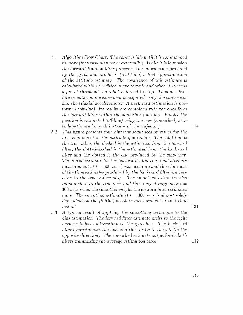
5.1 Algorithm Flow Chart: The robot is idle until it is commanded
to move (by a task planner or externally). While it is in motion
the forward Kalman lter processes the information provided
by the gyros and produces (real-time) a rst approximation
of the attitude estimate. The covariance of this estimate is
calculated within the lter in every cycle and when it exceeds
a preset threshold the robot is forced to stop. Then an abso-
lute orientation measurement is acquired using the sun sensor
and the triaxial accelerometer. A backward estimation is per-
formed (o-line). Its results are combined with the ones from
the forward lter within the smoother (o-line). Finally the
position is estimated (o-line) using the new (smoothed) atti-
tude estimate for each instance of the trajectory. . . . . . . . . 114
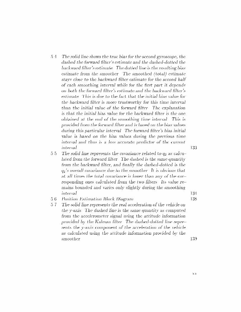
5.2 This gure presents four dierent sequences of values for the
rst component of the attitude quaternion. The solid line is
the true value, the dashed is the estimated from the forward
lter, the dotted-dashed is the estimated from the backward
lter and the dotted is the one produced by the smoother.
The initial estimate for the backward lter (i.e. nal absolute
measurement at t = 600 secs) was accurate and thus for most
of the time estimates produced by the backward lter are very
close to the true values of q1. The smoothed estimates also
remain close to the true ones and they only diverge near t =300 secs when the smoother weighs the forward lter estimates
more. The smoothed estimate at t = 300 secs is almost solely
dependent on the (initial) absolute measurement at that time
instant. . . . . . . . . . . . . . . . . . . . . . . . . . . . . . . 131
5.3 A typical result of applying the smoothing technique to the
bias estimation. The forward lter estimate drifts to the right
because it has underestimated the gyro bias. The backward
lter overestimates the bias and thus drifts to the left (in the
opposite direction). The smoothed estimate outperforms both
lters minimizing the average estimation error. . . . . . . . . . 132
xiv
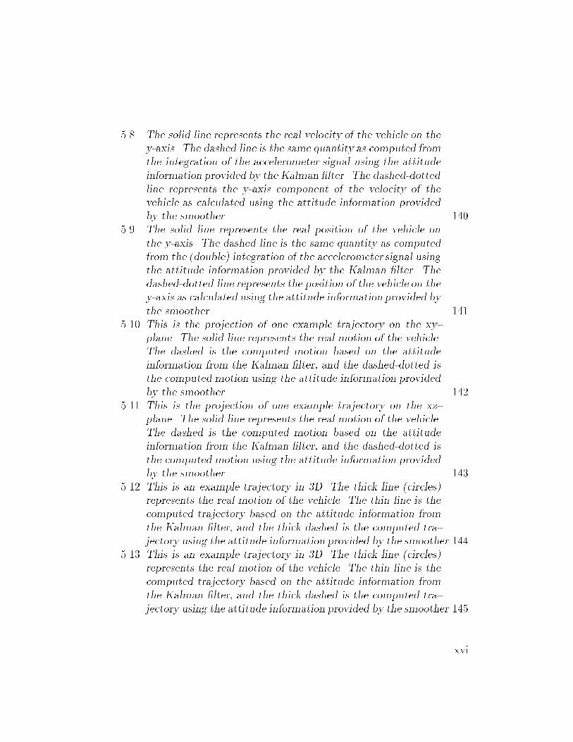
5.4 The solid line shows the true bias for the second gyroscope, the
dashed the forward lter's estimate and the dashed-dotted the
backward lter's estimate. The dotted line is the resulting bias
estimate from the smoother. The smoothed (total) estimate
stays close to the backward lter estimate for the second half
of each smoothing interval while for the rst part it depends
on both the forward lter's estimate and the backward lter's
estimate. This is due to the fact that the initial bias value for
the backward lter is more trustworthy for this time interval
than the initial value of the forward lter. The explanation
is that the initial bias value for the backward lter is the one
obtained at the end of the smoothing time interval. This is
provided from the forward lter and is based on the bias values
during this particular interval. The forward lter's bias initial
value is based on the bias values during the previous time
interval and thus is a less accurate predictor of the current
interval. . . . . . . . . . . . . . . . . . . . . . . . . . . . . . . 133
5.5 The solid line represents the covariance related to q2 as calcu-lated from the forward lter. The dashed is the same quantity
from the backward lter, and nally the dashed-dotted is the
q2's overall covariance due to the smoother. It is obvious that
at all times the total covariance is lower than any of the cor-
responding ones calculated from the two lters. Its value re-
mains bounded and varies only slightly during the smoothing
interval. . . . . . . . . . . . . . . . . . . . . . . . . . . . . . . 134
5.6 Position Estimation Block Diagram . . . . . . . . . . . . . . . 138
5.7 The solid line represents the real acceleration of the vehicle on
the y-axis. The dashed line is the same quantity as computed
from the accelerometer signal using the attitude information
provided by the Kalman lter. The dashed-dotted line repre-
sents the y-axis component of the acceleration of the vehicle
as calculated using the attitude information provided by the
smoother. . . . . . . . . . . . . . . . . . . . . . . . . . . . . . 139
xv
5.8 The solid line represents the real velocity of the vehicle on the
y-axis. The dashed line is the same quantity as computed from
the integration of the accelerometer signal using the attitude
information provided by the Kalman lter. The dashed-dotted
line represents the y-axis component of the velocity of the
vehicle as calculated using the attitude information provided
by the smoother. . . . . . . . . . . . . . . . . . . . . . . . . . 140
5.9 The solid line represents the real position of the vehicle on
the y-axis. The dashed line is the same quantity as computed
from the (double) integration of the accelerometer signal using
the attitude information provided by the Kalman lter. The
dashed-dotted line represents the position of the vehicle on the
y-axis as calculated using the attitude information provided by
the smoother. . . . . . . . . . . . . . . . . . . . . . . . . . . . 141
5.10 This is the projection of one example trajectory on the xy-
plane. The solid line represents the real motion of the vehicle.
The dashed is the computed motion based on the attitude
information from the Kalman lter, and the dashed-dotted is
the computed motion using the attitude information provided
by the smoother. . . . . . . . . . . . . . . . . . . . . . . . . . 142
5.11 This is the projection of one example trajectory on the xz-
plane. The solid line represents the real motion of the vehicle.
The dashed is the computed motion based on the attitude
information from the Kalman lter, and the dashed-dotted is
the computed motion using the attitude information provided
by the smoother. . . . . . . . . . . . . . . . . . . . . . . . . . 143
5.12 This is an example trajectory in 3D. The thick line (circles)
represents the real motion of the vehicle. The thin line is the
computed trajectory based on the attitude information from
the Kalman lter, and the thick dashed is the computed tra-
jectory using the attitude information provided by the smoother.144
5.13 This is an example trajectory in 3D. The thick line (circles)
represents the real motion of the vehicle. The thin line is the
computed trajectory based on the attitude information from
the Kalman lter, and the thick dashed is the computed tra-
jectory using the attitude information provided by the smoother.145
xvi
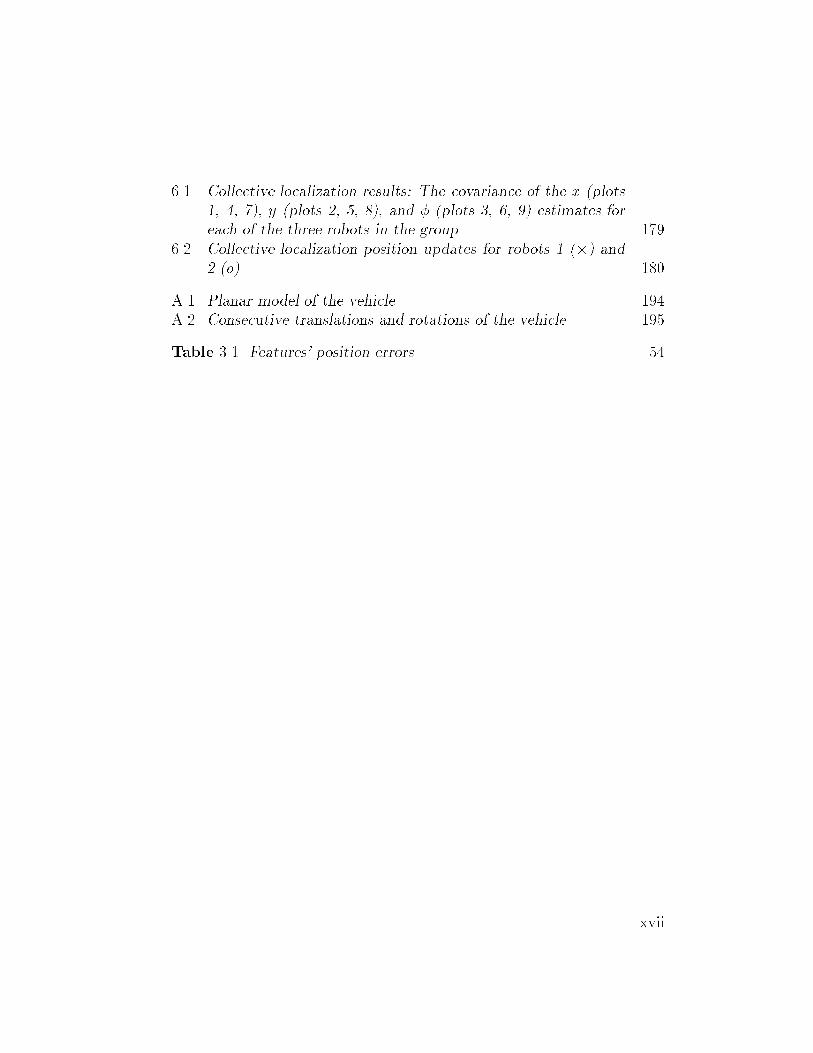
6.1 Collective localization results: The covariance of the x (plots
1, 4, 7), y (plots 2, 5, 8), and (plots 3, 6, 9) estimates for
each of the three robots in the group. . . . . . . . . . . . . . . 179
6.2 Collective localization position updates for robots 1 () and2 (o). . . . . . . . . . . . . . . . . . . . . . . . . . . . . . . . . 180
A.1 Planar model of the vehicle. . . . . . . . . . . . . . . . . . . . 194
A.2 Consecutive translations and rotations of the vehicle. . . . . . 195
Table 3.1 Features' position errors. . . . . . . . . . . . . . . . . . . . . 54
xvii
Abstract
Robust localization is the problem of determining the position of a mobile
robot with respect to a global or local frame of reference in the presence of
sensor noise, uncertainties and potential failures. Previous work in this eld
has used Kalman lters to reduce the eects of sensor noise on updates of
the vehicle position estimate or Bayesian multiple hypothesis to resolve the
ambiguity associated with the identication of detected landmarks. This dis-
sertation introduces a general framework for localization that subsumes both
approaches in a single architecture and applies it to the general problem of
localizing a mobile robot within a known environment. Odometric and/or
inertial sensors are fused with data obtained from exteroceptive sensors. The
approach is validated by solution of the \kidnapped robot" problem.
The second problem treated in this dissertation concerns the common
assumption that all sensors provide information at the same rate. This as-
sumption is relaxed by allowing high rate noisy odometric or inertial data
from kinetic sensors while absolute attitude and/or position data (e.g., from
sun sensors) are obtained infrequently. We address the resulting observability
limitation by incorporating a Smoother in the attitude estimation algorithm.
Smoothing of the attitude estimates reduces the overall uncertainty and al-
lows for longer traverses before a new absolute orientation measurement is
required. Simulation examples also show the ability of this method to in-
crease the accuracy of robot mapping.
xviii
The third problem concerns multiple robots collaborating on a single
task. In prior research with a group of, say M, robots the group localization
problem is usually approached by independently solving M pose estimation
problems. When collaboration among robots exists, current methods usually
require that at least one member of the group holds a xed position while
visual contact with all the other members of the team is maintained. If
these two conditions are not met, uncorrelated pose estimates can lead to
overly optimistic estimates. We introduce a new distributed Kalman ltering
approach for collective localization that overcomes the previous limitations
and combines optimally all available positioning information amongst the
members of a group.
xix
Chapter 1
Introduction and Problem Statement
1.1 Motivation
Mobile robots are fast becoming one of the most prominent applications of
robotics. They have moved from the factory oor and are now being sent
on missions to other planets [39], remote areas [96], or dangerous radioactive
sites [20]. The potential applications for mobile robots do not include only
special missions. They are also being used as guides in museums [91] and for
entertainment purposes [35]. In order for a mobile robot to travel from one
location to another it has to know its position at any given time. In most
cases today, this is achieved by either having a human in the navigation
loop [18] who directs the vehicle remotely or by constraining the robot to
operate in a certain area, precisely mapped [23], [91] or suitably engineered;
i.e. marked with beacons [51] or other articial landmarks [60].1 The level
of autonomy depends predominantly on the ability of the robot to know its
exact location using minimal a priori information about the environment,
represented in a simple way.
1From now on the words landmark and feature will be used interchangeably.
1
In order to navigate eectively, a robot must be able to quickly and ac-
curately determine its location. Fairly accurate position estimates can be
obtained by integrating kinetic information from the robot's proprioceptive
sensors (dead-reckoning). The error accumulation in these estimates when
traveling over long distances can lead to unacceptable performance. An ef-
fective way of observing the surroundings when the robot is uncertain of
its position estimates is by focusing on distinguishing characteristics of the
environment such as landmarks. A landmark is dened as a feature (or a
combination of features) of the environment that the robot's exteroceptive
sensors are capable of detecting. When a landmark is sensed the robot can
estimate its own pose2 by invoking information regarding the feature's pose3
with respect to some global frame. Two poor assumptions usually invoked by
existing localization schemes are that: (i) the world is populated with distinct
landmarks, and (ii) these can be sensed at all times. Finally, the increasing
need for robots working as teams has created the demand for algorithms
supporting cooperative localization of groups of mobile robots. Failure to
address the information inter-dependencies issue has led to schemes with un-
acceptable limitations: (i) At least one member of the group has to remain
stationary at all times, and (ii) visual contact between the stationary robot
and the rest of the group has to be sustained at all times.
2As pose we dene the position and orientation of the robot. For example, in the case
of a robot moving on a plane its position is determined by the pair (x; y) where x is the
displacement along the x-axis and y is the displacement along the y-axis with respect to
a global frame of reference. The orientation is usually denoted as and it describes the
cumulative rotation of the robot with respect to the global frame of reference. The pose
vector combines the position and orientation information in ~x = [x; y; ]0.3A known feature does not always provide information regarding all three degrees of
freedom x; y; . For example, stellar objects (e.g. the sun or stars [17]), the magnetic pole
of the earth, the gravitational center of the earth, the horizon, or objects in the horizon
(e.g. mountain peaks) can be used as landmarks that provide only attitude information
while the rest of the positional degrees of freedom remain undetermined.
2
1.2 Assumptions made in this Thesis
In this thesis we study the case of mobile robots that carry a variety of pro-
prioceptive sensors that monitor the motion of the vehicle. These sensors
can be accelerometers, gyroscopes, or their combination in an Inertial Nav-
igation System4(INS), wheel-shaft encoders, optical ow odometric systems,
Doppler radars, kinesthetic sensors etc. These devices are commonly found
as parts of dead-reckoning systems where the position of the robot is tracked
by integrating the kinetic information. The signals from these sensors con-
tain components of noise. In our case, the assumption made is that the noise
is Gaussian but it does not have to be zero-mean white. Shaping lters are
implemented to estimate on-line possible biases.
A robot is also equipped with exteroceptive sensors that monitor the en-
vironment for features. These sensors usually are sonars, laser scanners,
cameras (in single or stereo formation), compasses, sun sensors, star trackers
etc. There are two kinds of features that we exploit for localization purposes
and each of them provides a dierent level of localization information: (i)
Landmarks for position estimation, and (ii) Features for attitude estimation.
For the case of groups of robots the assumption made is that each of the
members of the group carries exteroceptive sensors for detecting other robots
of the same team and measuring their relative pose. Sensors with such capa-
bilities are stereo cameras and laser scanners. These robots are also assumed
to be capable of communicating with each other.
1.3 Problem Statement
This thesis addresses the following 3 problems:
4An Inertial Navigation System contains an Inertial Measurement Unit (IMU).
3
Problem 1: Given a map of the environment containing the poses of
similar appearing landmarks (feature identication uncertainty), com-
bine optimally, in the maximum a posteriori probability sense, the in-
formation from a feature detection module with the information pro-
vided by the robot's odometry, in order to globally localize the robot
(\kidnapped-robot" problem) and thus provide one or more initial loca-
tions for tracking the position of the robot thereafter.
Problem 2: When absolute orientation measurements are available to
the robot only intermittently (the attitude observability requirements
are satised only at certain time instants), determine the optimal, in
the minimummean-square error sense, sensor fusion scheme that com-
bines all the collected information, previous and current, to reconstruct
the attitude motion prole of the robot and provide the best possible lo-
calization accuracy as if all the measurements during this time interval
were available at once.
Problem 3: In the case of localization of groups of mobile robots,
determine the optimal, in the minimum mean-square error sense, co-
operative localization scheme that combines previously related (non-
independent) positioning information from dierent robots with cur-
rent relative pose measurements and compensates for the existing data
inter-dependencies without requiring that (i) at least one of the robots
is stationary at any given time, and (ii) all the robots sustain visual
contact with the stationary robot.
This thesis presents the following approaches for solving each of the previ-
ously stated problems:
4
Approach to Problem 1: In the case of similar appearing land-
marks used for position estimation, the exteroceptive sensors rst pro-
vide their data to the feature extracting module(s). Depending on
the identication capabilities of the feature recognition algorithm, one
or more possible matches with landmarks represented on an a priori
known map are returned along with their probabilities. The positions
of the candidate landmarks are processed within the proposed Multiple
Hypothesis Tracking framework. Most of the time, the resulting posi-
tion estimate for the robot is a collection of Gaussians produced using
a Kalman lter that tracks the position of the robot through a number
of possible paths, each containing a dierent set of landmarks. The
assumption of perfect landmark identication is relaxed.
Approach to Problem 2: In cases where attitude information is only
available intermittently (e.g. the objects that are being used as orien-
tation features are not in view or their signals are occluded or distorted
for long periods of time5), a robot has to integrate its rotational velocity
in order to estimate its orientation. Since the rotational velocity signals
are noisy, the resulting orientation estimates degrade with time. Ev-
ery time an absolute measurement is collected by exteroceptive sensors
capable of extracting orientation information from the environment,
instead of being processed by a Kalman lter that provides only the
current orientation estimate, it is fed directly into a Smoother that cal-
culates the current along with all the previous orientation estimates.
This way the attitude trajectory prole can be optimally reconstructed
using all the information available between the current and the previous
absolute orientation measurement.
5For example, a compass is very sensitive to the presence of metallic objects in the
vicinity.
5
Approach to Problem 3: When groups of two or more robots
are sensing each other and exchanging information in order to im-
prove their localization accuracy, the information exchanged during
a previous meeting can seriously aect the validity of their estimates.
It can become unrealistically over-optimistic. The information inter-
dependencies could be compensated by a centralized estimator that
would combine all the information collected by all the robots at all
times. Since such an estimator has very large communication and com-
putational requirements, it is desired to formulate this centralized esti-
mator so that it can be distributed amongst the robots. The resulting
scheme requires communication only when two robots sense each other.
6
Chapter 2
Literature Review
The following review contains representative examples of dierent approaches
to mobile robot localization.
2.1 Position Tracking
The errors associated with position tracking can be divided into two main
categories: (i) systematic and (ii) stochastic. Stochastic errors are due to
sensor noise while systematic errors are primarily due to errors in the values
of the parameters used to describe the system. For example, systematic er-
rors occur when the radii of the wheels of a robot are not known precisely
and they are assumed to be equal to a nominal value.
In order to deal with systematic errors which are particularly notable in
indoor applications, J. Borenstein and L. Feng present in [11] a calibration
technique called the UMBmark test. The dominant systematic error sources
are identied as the dierences in wheel diameter and the uncertainty about
the eective wheel base. By measuring the individual contribution of these
7
vehicle specic, dominant error sources, they counteract their eect in soft-
ware.
2.1.1 Position Tracking and Kalman ltering
Stochastic errors cannot be predicted or compensated o-line. Instead lter-
ing is introduced to estimate the values of the kinetic quantities of interest
in the presence of noise and combine their values in order to produce an esti-
mate of the position of the robot. Kalman ltering oers a powerful method
for low-level fusion in mobile robots, provided that the lter's modeling as-
sumptions can be satised, and that the uncertainty models that it requires
are available and reliable. The data integration process executed by the
Kalman lter is modular and can accommodate a large variety of sensory
measurements as long as the error covariance matrices are available. The
sequential processing of sensor data makes the Kalman lter a very exible
fusing mechanism that can process data from dierent sensors arriving at
dierent frequencies [85]. There exists a well-developed body of literature on
performance, stability and consistency of the lter, as well as tests for data
validation and performance consistency. These tests provide means to reject
spurious data on-line, and to check that state estimate errors satisfy certain
conditions on their statistics in spite of the use of approximations [3]. There
also exist dierent techniques for error compensation in linearized lters such
as the use of pseudo-noise covariance and compensation for bias in errors.
What follows is a representative group of eorts that focus on improving
the quality of the estimates when ltering is applied to position tracking. In
[12], the authors use measurements from odometric sensors (wheel encoders)
and INS (gyroscope) during dierent time intervals. Their method, gyrodom-
etry, uses odometry data for the majority of time, while substituting gyro
8
data only during brief instants (e.g. when the vehicle goes over a bump) dur-
ing which gyro and odometry data dier drastically. This way the system is
kept largely free of the drift associated with the gyroscope and compensates
for the non-systematic errors introduced by odometry. In [28], Y. Fuke and
E. Krotkov use a complementary Kalman lter introduced in [15] to estimate
the vehicle's attitude from the accelerometer signal in low frequency motion
and the gyro signal in high frequency motion. The attitude information is
then used to calculate the rotational transformation matrix from the vehicle
coordinate system to the ground coordinate system. This matrix transforms
the velocity information to a position increment. In [4], the authors use a low
cost INS system (3 gyroscopes, a triaxial accelerometer) and 2 tilt sensors.
Their approach is to incorporate in the system a priori information about
the error characteristics of the inertial sensors and to use this information
directly in an Extended Kalman Filter (EKF) to estimate position before
supplementing the INS with absolute sensing mechanisms. The main draw-
backs of this work are that the statistical assumptions for the accelerations
are not justied and the orientation information is missing in the calculation
of the position.
2.1.2 Position Tracking and Landmarks
Landmark-based approaches rely on the recognition of features to keep the
robot localized geometrically. Landmarks may be given a priori (for ex-
ample passive or active beacons) or learned by the robot as it maps the
environment. While landmark methods can achieve impressive geometric lo-
calization, they require either engineering of the environment to provide an
adequate set of known landmarks, or ecient recognition of features to be
9
used as landmarks1.
If a robot carries only proprioceptive sensors that monitor the motion of
the vehicle, then the position of the robot is not observable. This means that
the Kalman lter estimate will drift away from a precise position estimate
unless absolute position information is available to the robot at frequent
intervals. Most of the current research eorts incorporate some form of ex-
teroceptive information in order to update the position estimate and thus
keep the uncertainty bounded. This usually requires engineering of the en-
vironment with articial landmarks or beacons. Work related to absolute
localization is presented by J. J. Leonard and H. F. Durrant-Whyte. In [51]
they develop a system in which the basic localization algorithm is formalized
as a vehicle-tracking problem, employing an Extended Kalman lter (EKF)
to match beacon observations (environment features) to a navigation map to
maintain an estimate of the position of the mobile robot. In [7], the authors
also use an EKF in order to fuse odometry and angular measurements of
known landmarks (light sources detected using a CCD camera). In [5], E. T.
Baumgartner and S. B. Skaar estimate a vehicle's position and orientation
based on the observation of visual cues located at discrete positions within
a structured environment. An EKF is used to combine these visual observa-
tions with sensed wheel rotations in order to continuously produce optimal
estimates.
In another approach to the position tracking problem supported by maps
of the environment, instead of Kalman ltering, the SPlter is introduced
[61]. In this paper the authors use a version of the symmetries and per-
turbation model method to process uncertain geometric information from a
1A robot can use a feature for updating its position if that corresponds to a unique
location in the map. This means the robot has to be capable of discriminating between
similar appearing landmarks. Failure to reliably identify which landmark is in sight will
prevent the robot from exploiting this potential source of information.
10
monocular camera and a laser range-nder. Information provided by the
laser sensor is used both to determine the location of walls in front of the
robot and, by processing the intensity image, to determine the location of
vertical edges that can correspond to corners, as well as door and window
frames. Odometry is used to predict the location of walls and edges. Match-
ing of these elements with an a priori map of the environment provides the
required correction to the degrading odometry. Initial estimate of the po-
sition of the robot is necessary for the initialization of the algorithm. The
correspondence between elements on the map and elements that the robot
senses is based on vicinity criteria. When there is more than one candidate
for this pairing, the measurement is discarded.
Most of the previous techniques for localization focus on optimizing po-
sition tracking. These methods fail when a precise initial estimate of the
position of the robot is not available. In addition, these algorithms cannot
deal with cases where the environmental features appear to be identical.2
The decision for the identity of a landmark has to be made immediately and
it is based on the current position estimate of the robot and the topology of
the landmarks. The nearest neighbor is assumed to be the feature detected.
If more than one identical features are in the same area - the size of which
is determined according to the uncertainty of the current position estimate
of the vehicle - this information is discarded by the robot. These approaches
depend on the estimate of the displacement of the robot between consecutive
landmarks in order to match observed features to features on a given map.
Should this estimate becomes unreliable, due to error accumulation, the robot
is not able to produce the 1-to-1 correspondence between locations it travels
2Two landmarks appear to be identical if the feature extraction module is not able
to distinguish them based on the information provided from the exteroceptive sensors
available to the robot.
11
through3 and locations on the map, required for a successful position update.
2.2 Absolute Localization
In this family of approaches the initial position of the robot is assumed to be
unknown and has to be determined by the robot based on information from
maps of the environment. In some cases landmarks are used and in others a
grid-based description of the area is involved.
2.2.1 Absolute Localization and Landmarks
One category of landmark based mobile robot localization approaches relies
on angular measurements of known but indistinguishable landmarks [38].
The assumption is that 3 landmarks have to be in sight at all times. For
example, in [87], Sugihara addresses a version of the localization problem
where the points in the environment look identical. The robot measures the
direction of rays emanating from the robot's position through an observed
point. Sugihara gives an O(n3 log(n)) algorithm for nding the robot's po-
sition and orientation such that each ray pierces at least one of the n points
in the environment. Avis and Imai [2] and Krotkov [44] extend Sugihara's
results to the case that angle measurements include errors. In [44], the robot
is equipped with a CCD camera and is assumed to move on a at surface.
A map of the environment is available to the robot. The camera extracts
vertical edges from the environment. These edges do not contain enough
3The landmarks have to appear in front of the robot frequently enough so that a
correspondence with the map can be made before the tracking estimate degrades to the
point that more than one features on the map could be what the robot detects.
12
information to determine locally which vertical edge corresponds to which
point in the map. The problem is to identify the position and orientation of
the robot by establishing the correspondence between the directions of the
vertical edges and points on the map. This approach avoids the 3D recon-
struction and the feature identication problem. It is formulated as a search
in a tree of interpretations [33] (pairings of landmark directions and land-
mark points). An algorithm to search the tree eciently is developed taking
into account errors in the landmark directions extracted by image processing.
The main drawbacks of this algorithm are the time requirements O(n4) and
its inability to deal with spurious measurements. Only the worst case in the
accuracy of the estimate is calculated and it lacks the ability to incorporate
information provided by odometry.
In [6], the landmarks are considered to be distinguishable. This paper
deals with the problem of how to relate robot-centered information with
global-centered information in an environment with landmarks. The assump-
tion is that the robot can detect these landmarks and measure their bearings
relative to each other. The map of the environment is used to determine the
location of the robot. This is another triangulation approach. At least 3
landmarks have to be in sight in order to estimate the position of the robot.
The algorithm presented assumes that more than 3 landmarks are available
and thus the system is overdetermined. Least squares estimation is applied
and the major contribution of the suggested method is that the derived al-
gorithm is linear in the number of landmarks. Similarly, in [88], the authors
also use distinguishable landmarks of the environment. The focus of this
paper is to show that for a certain error in the angle measurement, the local-
ization error varies depending on the conguration of the landmarks. In [89],
a Neural Network-based approach is presented to the problem of learning
the most suitable, distinguishable landmarks for mobile robot localization.
13
The choice of a landmark as useful depends on the improvement in the belief
level for the position of the robot in an oce environment. During each step
of the training, the presented algorithm assumes an initially uniform belief
function centered around the position of the landmark under investigation.
The results presented are for the best case when the initial belief function for
the robot's position is the same as the one used during the training phase.
Another key limitation of this approach is that it does not learn the loca-
tions of the landmarks ((x; y) coordinates). It only learns to associate sensor
readings with locations that the robot visits.
A more qualitative approach is presented in [53]. Long surfaces such as
walls and corridors are used as topological primitives for localization and
mapping. Each of the landmarks detected is identied based on its type (left
wall, right wall, corridor), rough size and approximate position and orien-
tation. All these criteria used to compare landmarks are either qualitative
or approximate. There is no probabilistic interpretation of their similarities
and a decision has to be made immediately after a feature is detected. It is
either decided that it is the same as another landmark previously detected
and stored in a map, or it is assumed to be a new feature of the environment.
There is no notion of the condence level related with each decision made.
Another drawback of this approach is that it does not allow for more than
one hypothesis for the location of the robot to exist and thus the decision
cannot be postponed for a later time when more information is available. Fi-
nally, the graph connectivity used for the landmark disambiguation depends
heavily on precise knowledge of the robot's orientation and cannot be used
if this transition has not been done before.
14
2.2.2 Absolute Localization and Dense Sensor Maps
Dense Sensor methods [34] attempt to use whatever sensor information is
available to update the robot's position. They do this by matching dense
sensor scans against a surface map of the environment, without extracting
landmark features. Thus, dense sensor matching can take advantage of what-
ever surface features are present, without having to explicitly decide what
constitutes a landmark.
Markov Localization uses a discrete representation for the a priori and a
posteriori probabilities of the position of the robot. A grid map or topological
graph covers the space of robot poses and a probability is assigned to each
element of this space. The key idea is to compute the discrete approxima-
tion of a probability distribution over all possible poses4 in the environment.
The area around the robot has to be updated at every step to provide the
new probabilities for each cell for the robot to be there. Computationally
this technique depends on the dimensionality of the grid and the size of the
cells. The main advantage of this technique is that it is capable of localizing
the robot even when its initial position is unknown. This is essential for an
autonomous robot since its initial position need not be given when the robot
is switched on or if it gets lost due to an accident or a failure. These meth-
ods can be categorized according to the type of discretization they rely on.
In most cases5, a ne-grained grid-based approximation of the environment
is used to calculate the distribution of the robot's position. In these cases
metric maps of the environment are used. These can be CAD maps that
consist of line segments or occupancy grid maps. In all cases the map is used
4Pose denotes position and orientation.
5In some cases a topological discretization of the environment is used. Landmarks are
detected to localize the robot and the assumption commonly made is that these areas
(landmarks) are distinguishable.
15
to compute what the sensor readings should be from a given cell in the state
space. For example, in [90], a probabilistic grid-based algorithm is used for
localization while a topological map is derived for the path planning task.
The main drawbacks of this method, namely large memory and processing
requirements, are due to the grid-based representation of the area. Another
disadvantage is that the accuracy of the method depends on the size of the
grid used. The method lacks the ability to optimally fuse dierent sources of
proprioceptive sensor information and capitalize in the existing framework
of Kalman ltering based position tracking approaches.
Kalman ltering can be applied to the case of Dense Sensor methods [34].
Scan matching (model matching) is performed by rotating and translating
every range scan in such a way that a maximum overlap between the sensor
readings and the a priori map emerges. The advantage of this method is
that it can globally localize the robot precisely given accurate inputs. The
main drawback of the approach is the number of computations required for
the model matching. A reasonable solution would be to incorporate odom-
etry and based on the odometric estimate of the position of the robot, to
limit the search to small perturbations of the sensor scans of the area that
is visible from the current position of the robot and discard the non-visible
areas. Though this approach reduces the required number of computations,
it sacrices the ability to globally localize the robot, i.e. when its initial
position is unknown.
16
2.3 Rule Based Sensor Fusion
The methods previously reported rely on well dened uncertainty models,
and execute variants of maximum likelihood or maximum a posteriori esti-
mation. Such models are dicult to develop when the navigation depends
on patterns and signatures on the map (e.g. landmarks). Often they are
also dicult to obtain for data that are combined from sensors that use sig-
nicantly dierent principles and processing techniques. When uncertainty
models are either unavailable or are meaningless, ad hoc techniques have of-
ten been used within the domain of sensory data. In almost all cases, the
advantage of a sound formal basis is lost, though several attempts were made
to provide alternative \unied" frameworks in these situations. It is instruc-
tive to point out that in spite of their seemingly dierent procedures, most of
these frameworks still execute the same prediction, observation, validation,
and updating cycle used by the Kalman lter.
Rule-Based Sensor Fusion: To avoid the diculty in modeling sensor
readings under a unied statistical model, several robotic applications use
rule-based algorithms. Often these algorithms do not require an explicit
analytical model of the environment. Expert knowledge of the sensors' char-
acteristics and prior knowledge about the environment are used in the design
of feature extraction, mapmaking, and self localization techniques. The re-
sulting rules, after some experimentation, are usually simple and robust.
The obvious disadvantage is limited domain of applicability - the insights to
create rules for a specic environment cannot be exported easily to other en-
vironments. Changes in the sensor suite and in the environment may require
re-evaluation and re-compilation of the rule set. In [26], Flynn developed a
simple set of heuristic rules for a robot that uses an ultrasonic sensor and a
near-infrared proximity sensor. Ultrasonic sensors have wide angles but give
17
relative accurate range measurements. Infrared sensors have excellent angu-
lar resolution but poor distance measurements - they are therefore well-suited
for detection of edges and large depth discontinuities such as doorways. Fu-
sion of measurements from both ultrasonics and infrareds has the potential
to provide robots with good readings in both range and angular position. A
set of rules has been used by Flynn to validate the data from the sensors
and to determine which sensor to rely upon when con icting information is
obtained. Using these simple rules, the original sonar boundary was redrawn
to take into account features that were found by the near-infrared sensor.
Signicant improvement in the mapping of a laboratory environment was
demonstrated in [26].
2.4 Multiple Hypothesis Testing
2.4.1 Previous Approaches
To the best of our knowledge the only applications of a Multiple Hypothe-
sis approach in mobile robots are presented in [16] and [52]. In both cases
the Multiple Hypothesis Testing framework is employed in order to deduce
the origin of sonar data. Two dierent formulations of a Kalman lter are
involved. One is tuned to re ections from a corner and the second to re-
ections from a planar surface. In the focus of both these approaches is the
data association problem [45]. A dierent Kalman lter (one of the two types
mentioned) is used for each new feature. As a result, the number of potential
hypotheses grows fast in time and there is a need to provide active and eec-
tive management of candidate hypotheses in order to limit the computation
involved in developing identity and location estimates. Thresholding of the
18
innovation (residual) is used to decide if a measurement originated from a
certain target. The selection of the threshold is ad hoc. Another drawback
is that odometric information is not considered at all. At the same time,
the location and orientation of the vehicle is supposed to be precisely known
at any time. The procedure involved in constructing the hypothesis matrix
required in this algorithm is based on the assumption that each measurement
has only one source and each geometric feature has at most one associated
measurement per scan. In other words, geometric features that produce more
than one measurement in a single data set are excluded. This causes loss of
useful information. The main limitation of this approach is that by applying
multiple hypothesis estimation on low level data, such as single scans from
sonar sensors, limits its application to the case of corners and at surfaces
only. It is not obvious how other types of sensors or features can be incor-
porated in the same framework.
2.4.2 Proposed Extensions to Mobile Robot Localization
Following a dierent trail of thought, we intend to reformulate the Multiple
Hypothesis approach to develop a robust and reliable framework for mobile
robot localization. The proposed method overcomes a number of limitations
of the previous approaches. In this framework, the data to be combined are:
(i) relative position estimates as these result from a Kalman lter that op-
timally fuses the information from the proprioceptive sensors to keep track
of the position of the robot and (ii) absolute position measurements that re-
sult from processing the raw exteroceptive sensor data in a variety of feature
extracting modules and using previous knowledge of the environment stored
into maps of the area. Consequently, our method is modular and expand-
able to any number and type of sensors and features. This adds exibility to
19
the system since dierent robotic systems are equipped with dierent sets of
sensors and dierent types of environments are populated by dierent types
of features.
Another advantage of the proposed method is that it can deal with cases
of landmarks that look similar. Each possible landmark initiates a new hy-
pothesis. The number of hypotheses is kept small by incorporating the odo-
metric information in the decision process. Relative position information is
sucient to resolve the ambiguity about the identity of a landmark when
sucient time is allowed. The proposed Multiple Hypothesis Tracking algo-
rithm produces estimates of the position of the robot at all times starting
from an initial uniform position distribution. Each of the hypotheses created
contains a separate history of the topological transitions of the robot
through dierent landmark sites.
One of the drawbacks of Kalman lter estimation is that it can only
represent unimodal distributions approximated by a single Gaussian. The
proposed Multiple Hypothesis Tracking framework is capable of sustaining
more than one hypothesis for the position of the robot. Each of these hy-
potheses is represented as a Gaussian distribution. Thus, multi-modal dis-
tributions can be represented and approximated by an arbitrary collection
of Gaussians.6 Another advantage of the proposed method is that for any
number of hypotheses, only one Kalman lter is required to propagate
the position estimate and update it when a new landmark appears.
Our approach can rely solely on the detection of structural features of
the environment such as doors, windows, corners, poles, corridors, etc. Com-
pared to the grid-based approaches it is robust to dynamic environments
6In the limit, any distribution can be approximated by a collection of Gaussians.
The quality of the approximation depends mainly on the number of the Gaussians used
for the approximation.
20
since it does not depend on a detailed map of the area that should include
objects of small size that usually are part of the ever changing clutter. In-
stead we prefer to use a coarse scale map composed of reliably detectable
features and their position with respect to some global frame.
Kalman ltering is more accurate when sucient sensor information is
available from the sensors. On the other hand, Markov localization (that
uses Bayesian Estimation) is more robust and is capable of localizing a robot
in an arbitrary probabilistic conguration (when the initial position of the
robot is not known). Kalman ltering uses a more compact representation
for the uncertainty of the position of the robot and thus the propagation of
this uncertainty is very ecient. In the next chapter we present the proposed
method that combines the robustness of Markov localization and the
eciency and accuracy of Kalman ltering.
21
Chapter 3
Bayesian Estimation and Kalman Filtering:
Multiple Hypothesis Tracking
3.1 Introduction
The localization problem for a mobile robot consists of its ability to answer
the question \Where am I?", with respect to a given set of reference coordi-
nates. This problem could be solved if the area in which a robot moves could
be marked in a unique separable way. That means each place should contain
information that will make it recognizable and distinguishable from all other
places in the area. A rst approach to the problem would require each loca-
tion to have a unique \signature". This signature may be provided directly
or calculated with the aid of an external source. This is already available
for some areas where the Global Positioning System (GPS) signals are avail-
able. The triangulation of the distances from the satellites in view assigns a
unique pair of numbers to each location on the surface of the planet, namely
the longitude and latitude. Longitude and latitude are the geographical co-
ordinates that are used for long distance navigation of airplanes, ships and
even cars. This attractive method suers from a wide variety of problems.
The rst and most important one is the accuracy of the signals. Even some
22
of the most expensive commercial GPS devices provide an accuracy of a few
centimeters which is more than enough when a car drives from one side of a
city to the other but it is not acceptable for robots that move in cluttered
environments or handle material located within small distances. Another
serious drawback is that the GPS signals are not available indoors or in the
vicinity of tall buildings, bridges and structures that occlude the view of the
necessary number of satellites. Finally, the cost of a GPS receiver is too high
for many robotic applications.
In many scenarios where GPS is not available, the signature of a loca-
tion has to be determined based on the distinguishing characteristics of the
area itself. In this case the dissimilarity between signatures of dierent lo-
cations has to be identiable by the sensors used for this reason. There are
many attributes of the environment that can be exploited to gain signature
diversity. These can be dynamic or static. Temperature, chemical consis-
tency of the air, light and sound conditions belong in the rst category and
though they can be measured accurately, are not appropriate for marking an
area. This is because neighboring locations tend to have similar values for
the same quantities. In addition, these values can change with respect to
time in an unpredictable or dicult to model fashion. More static character-
istics need to be detected in order to provide distinctive \signatures". The
color and the shape of a location are strong candidates for discriminating
dierent areas and tend to remain unchanged over long periods of time. Vi-
sual memorization of each place may be sucient for distinguishing between
them. Although the homing capabilities of many types of insects [14], [94]
and other animals [31], [24] depend on this type of localization, serious im-
plementation issues have to be resolved before this technique can be applied
to mobile robot localization. The requirements for storing and processing
the numerous collected images are probably the most dicult to overcome.
23
Another way to achieve the desired distinguishability of a location of con-
cern is by preparing a detailed volumetric map of the area and then matching
the information from exteroceptive sensors with the information stored in the
map. This approach suers from the following drawbacks: (i) The prepara-
tion of the map adds signicant overhead to the process. It has to be full,
exhaustive, and precise enough to exclude any ambiguities and avoid mis-
interpretation, (ii) The exteroceptive sensors have to be able to supply the
robot with the same level of detail as that imprinted on the map. A laser
scanner is a good example of such a device. The cost of such sensors is
prohibitive for many mobile robot applications, (iii) The processing require-
ments to obtain the necessary information and match it to the corresponding
locations on the map call for a powerful processor on-board the robot if real-
time operation is demanded. This adds further expenses to the cost of this
approach.
Instead of building elaborate detailed maps of the entire environment, an
alternative would be to compose a topological map of the area where sep-
arate locations are described in terms of the actions or directions required
for a robot to follow in order to transfer from a known initial location to
the desired one. This can be seen as creating a graph of the area where the
nodes are locations of interest and the arcs contain descriptions for the tran-
sitions. These directions are usually described in terms of the capabilities of
the particular vehicle. A more unifying description of the topology would be
to use the metric distances between two locations of interest. Although this
approach allows one to abstract from the robot currently utilized, it intro-
duces extra problems such as path planning and motion control. In addition,
a mobile robot is capable of distinguishing between adjacent areas only if it
can precisely track its own position. Regardless of how the map was derived,
24
the vehicle is considered capable of following designated paths. This is con-
ditioned on the robot's ability to estimate at all times its displacement with
respect to some initial or intermediate locations.
Most current localization eorts have focused on supporting high qual-
ity displacement estimates (pose tracking). Dierent sensing devices and
odometric techniques have been exploited for this purpose. The common
characteristic of these approaches is that they rely on the integration of
some kinetic quantity. The main drawbacks of any form of odometry are:
1) Every sensor monitoring the motion of the vehicle has a certain type and
level of noise contaminating its signal. Integration of the noisy components1
causes gradual error accumulation and makes the estimates untrustworthy.
2) The kinematic model of the vehicle is never accurate. For example, we do
not know with innite precision the distance between the wheel axes of the
vehicle. 3) The sensor models also suer from inaccuracies and can become
very complicated. For example, the use of complicated models to describe
the gyroscope drift. 4) The motion of the vehicle involves external sources
of error that are not observable by the sensors used. For example, slippage
in the direction of motion or in the perpendicular direction is often not de-
tected by the motion sensors. Externally provided or extracted information
is necessary from time to time if we wish to keep the error bounded. This
group of approaches is also referred to as dead-reckoning2 and we will revisit
them in more detail in the following sections.
After brie y reviewing some of the marking strategies that could be ex-
ploited by a variety of localization algorithms, it is obvious that determining
1In particular, the noise associated with the rotational velocity measurement causes
large errors in the position estimate and those errors do not average to zero over some
period of time.2Sensors used for measuring kinetic quantities such as velocity, acceleration, etc will
be referred here as kinetic or proprioceptive sensors. Amongst these are odometric sensors
such as wheel encoders or inertial sensors such as gyroscopes and accelerometers.
25
the position of the robot is not an easy task for any of these approaches.
In this thesis we present a scheme that relies on a combination of dierent
types of \signatures" in order to distinguish between dierent places. This
scheme constitutes a exible, more robust and easier to implement solution
to the localization problem. For instance, instead of reproducing on a de-
tailed map all the surroundings of a robot for each area of interest, it is
desirable to attempt to create a more compact representation, i.e. to extract
the minimal information that makes a location unique with respect to other
locations. This is not necessarily restricted to the particular attributes that
a certain spot has. It can be generalized to include information for this loca-
tion with respect to its displacement from other known or previously visited
sites. More specically, the discrimination requirement can be approached
by considering not only \What does this location look like" but also \How do
I get to this location".
If, for example, a robot is capable of distinguishing two fairly similar
doors just by looking at them (as humans do by reading a sign on a door)
then the problem is essentially solved. This is one of the prominent ways that
humans use to recognize their location. Certain aspects of dierent locations
are compiled in a compact form of mnemonic representation. Not all the
information is preserved, which sometime makes it unreliable. Our ability to
distinguish between one place or another is not unlimited. There are certain
cases where the memory is not developed enough to support an unambiguous
decision or prevent a mistake. This problem is even more prevalent in arti-
cial machines such as robots equipped with sensing devices like a camera, for
example. The state of the art of pattern recognition techniques is far from
being able to mirror the perceptual and processing capabilities of the human
eye.
26
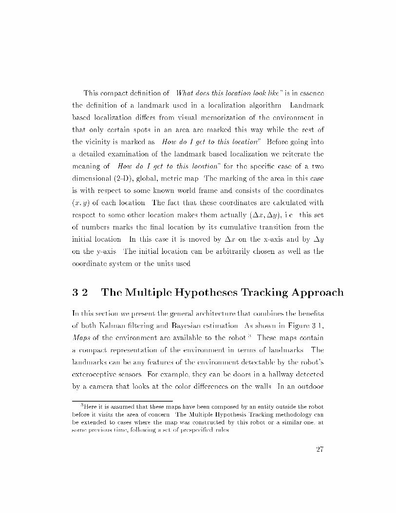
This compact denition of \What does this location look like" is in essence
the denition of a landmark used in a localization algorithm. Landmark
based localization diers from visual memorization of the environment in
that only certain spots in an area are marked this way while the rest of
the vicinity is marked as \How do I get to this location". Before going into
a detailed examination of the landmark based localization we reiterate the
meaning of \How do I get to this location" for the specic case of a two
dimensional (2-D), global, metric map. The marking of the area in this case
is with respect to some known world frame and consists of the coordinates
(x; y) of each location. The fact that these coordinates are calculated with
respect to some other location makes them actually (x;y), i.e. this set
of numbers marks the nal location by its cumulative transition from the
initial location. In this case it is moved by x on the x-axis and by y
on the y-axis. The initial location can be arbitrarily chosen as well as the
coordinate system or the units used.
3.2 TheMultiple Hypotheses Tracking Approach
In this section we present the general architecture that combines the benets
of both Kalman ltering and Bayesian estimation. As shown in Figure 3.1,
Maps of the environment are available to the robot.3 These maps contain
a compact representation of the environment in terms of landmarks. The
landmarks can be any features of the environment detectable by the robot's
exteroceptive sensors. For example, they can be doors in a hallway detected
by a camera that looks at the color dierences on the walls. In an outdoor
3Here it is assumed that these maps have been composed by an entity outside the robot
before it visits the area of concern. The Multiple Hypothesis Tracking methodology can
be extended to cases where the map was constructed by this robot or a similar one, at
some previous time, following a set of prespecied rules.
27
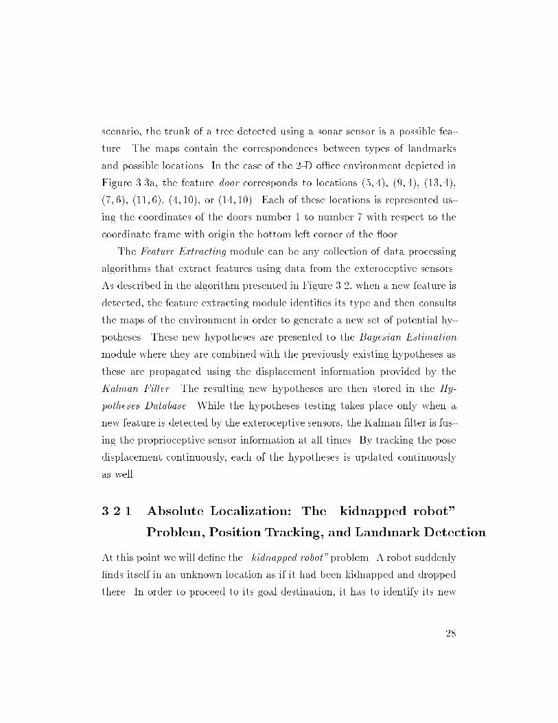
scenario, the trunk of a tree detected using a sonar sensor is a possible fea-
ture. The maps contain the correspondences between types of landmarks
and possible locations. In the case of the 2-D oce environment depicted in
Figure 3.3a, the feature door corresponds to locations (5; 4), (9; 4), (13; 4),
(7; 6), (11; 6), (4; 10), or (14; 10). Each of these locations is represented us-
ing the coordinates of the doors number 1 to number 7 with respect to the
coordinate frame with origin the bottom left corner of the oor.
The Feature Extracting module can be any collection of data processing
algorithms that extract features using data from the exteroceptive sensors.
As described in the algorithm presented in Figure 3.2, when a new feature is
detected, the feature extracting module identies its type and then consults
the maps of the environment in order to generate a new set of potential hy-
potheses. These new hypotheses are presented to the Bayesian Estimation
module where they are combined with the previously existing hypotheses as
these are propagated using the displacement information provided by the
Kalman Filter. The resulting new hypotheses are then stored in the Hy-
potheses Database. While the hypotheses testing takes place only when a
new feature is detected by the exteroceptive sensors, the Kalman lter is fus-
ing the proprioceptive sensor information at all times. By tracking the pose
displacement continuously, each of the hypotheses is updated continuously
as well.
3.2.1 Absolute Localization: The \kidnapped robot"
Problem, Position Tracking, and Landmark Detection
At this point we will dene the \kidnapped robot" problem. A robot suddenly
nds itself in an unknown location as if it had been kidnapped and dropped
there. In order to proceed to its goal destination, it has to identify its new
28
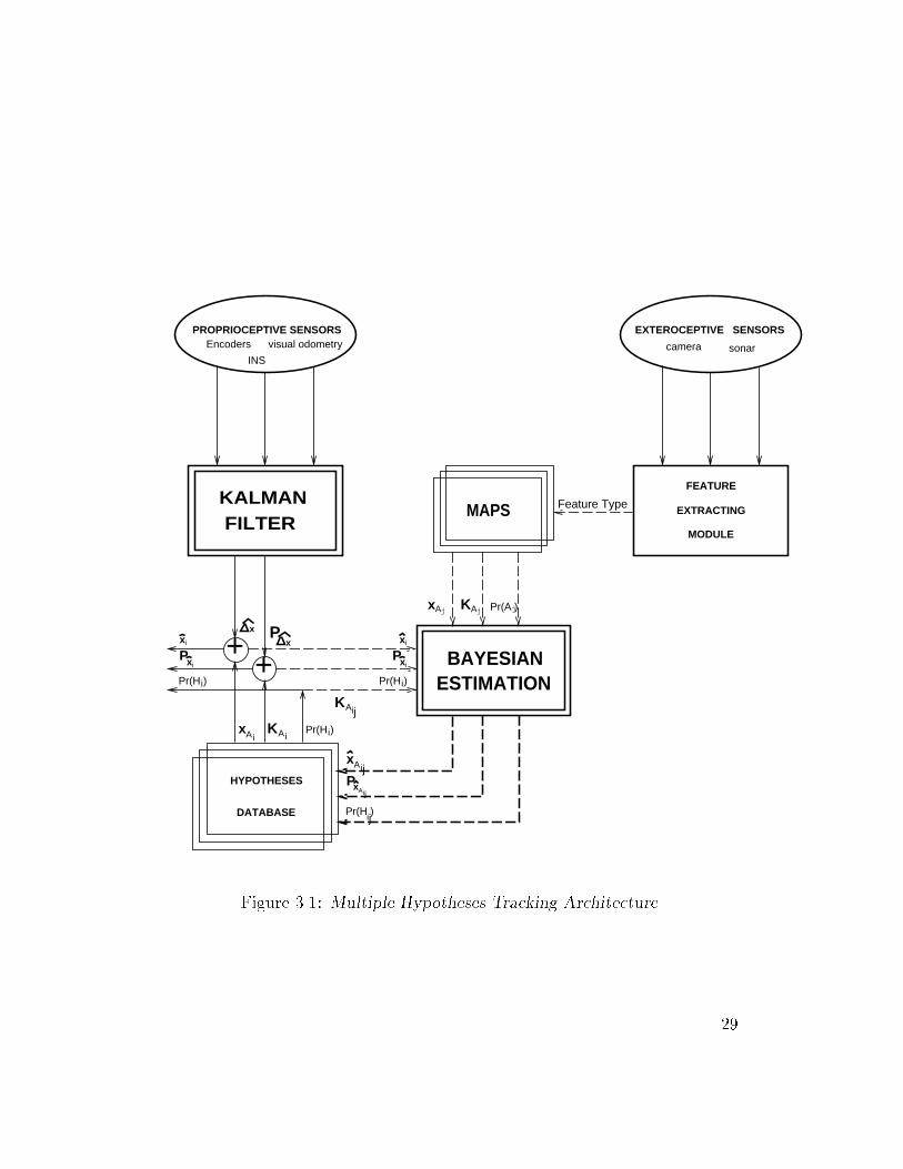
Encoders
INS
visual odometry
MAPSFILTERKALMAN
BAYESIANESTIMATION
PROPRIOCEPTIVE SENSORS
FEATURE
EXTRACTING
MODULE
EXTEROCEPTIVE SENSORS
camera sonar
KAjxAj Pr(A )j
HYPOTHESES
DATABASE
Pr(H )iPr(H )i
++
Px
xAi AiK Pr(H )i
xi
xiP
x
ix
xiP
Feature Type
AKij
Pr(H )ij
xAijxAij
P
Figure 3.1: Multiple Hypotheses Tracking Architecture.
29
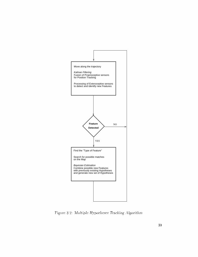
Feature
Detected
Combine possible new Featureswith previously existing Hypothesesand generate new set of Hypotheses
Bayesian Estimation
Find the "Type of Feature"
Search for possible matcheson the Map
YES
NO
Kalman FilteringFusion of Proprioceptive sensorsfor Position Tracking
Move along the trajectory
Processing of Exteroceptive sensorsto detect and identify new Features
Figure 3.2: Multiple Hypotheses Tracking Algorithm.
30
position. Maps of the environment are available to the robot. The challenge
is to design a localization scheme that will enable the robot to determine
its location on the map by searching around and exploiting its sensing capa-
bilities. The ability of the robot to recognize its location is very important
because it allows a robot to recover from an accident and thus increases its
reliability. For example, if a robot while moving along its path is hit by
something and pushed to a new location, it should be able to determine its
new position and continue with its tasks. In addition, the rst time that a
robot is brought into a new area, it is desirable that it can nd its initial
location without external help.
The absolute localization problem can be dened as threefold:
1. The robot determines its initial position (\kidnapped robot" problem),
2. The robot continuously tracks its position, and
3. The robot updates its deteriorating position tracking estimates by de-
tecting new features in the environment.
Before presenting the implemented approach to the general localization prob-
lem, we rst study the ideal case of a robot equipped with exteroceptive
sensors capable of distinguishing between almost identical landmarks and
restricted to move within a certain area. Though this scenario is ctional,
it will ease the transition to the more realistic case of imperfect landmark
recognition and imperfect odometry.
31
3.2.1.1 Perfect Landmark Recognition, Imperfect Odometry
In the absence of any previous knowledge, the robot's initial position dis-
tribution can be assumed to be uniform and thus the probability density
function (pdf) is:
f0(x) =1
S; (3.1)
where S is the surface of the area that the robot is allowed to move in and
x = [x ; y]T is the position of the robot. In the case of perfect landmark
recognition, there is no ambiguity. The decision is binary for each of the
possibilities encountered:
P (zk = Ai) = 1 ; P (zk = Aj) = 0 ; j = 1; :::; N; j 6= i ; (3.2)
whereAi is the encountered landmark and zk is the kth measurement provided
from the exteroceptive sensors.4 Every time the robot detects and identies
a landmark whose exact position xAiis known, the updated pdf becomes:
f(x=zk) = f(x=zk = Ai) = (x xAi) ; (3.3)
where is the Dirac delta, or, in the case that the position of the landmark is
known to follow a Gaussian distribution with mean value xAiand covariance
KAi:5
f(x=zk) = f(x=zk = Ai) =
4Actually zk is the result of processing the data from the exteroceptive sensors within
the feature extracting module.5For the 2D case KAi
= [2xAi
0 ; 0 2yAi
]
32
1
(2)n=2
det(KAi)1=2
exp[1
2(x xAi
)TKAi
1(x xAi)] (3.4)
where
KAi= E[(x xAi
) (x xAi)T ] (3.5)
The Gaussian assumption for the distribution of the position of the landmark
is often invoked to represent the spatial uncertainty of the measurements pro-
vided from the exteroceptive sensing devices. The sensors used to locate the
position of a landmark have limited precision and their signals are in general
noisy. Therefore, the calculation of the position of the landmark with respect
to the current position of the robot has its own inaccuracies. A Gaussian
model can be used to describe the uncertainty of the calculated transforma-
tion from the egocentric frame to the allocentric (landmark-centered) frame.
Every time a landmark is left behind, the robot knows its location pre-
cisely. The pdf of its position is a Gaussian function of its coordinates in the
area. This distribution is unimodal since we have assumed a 1-to-1 match
between encountered landmarks and locations on the map. From then on
the robot has to rely on its odometry until it encounters another landmark.
In the absence of any external positioning information, the uncertainty of
the position estimate will increase continuously as the robot moves. The
system is not observable6 and thus any estimation technique will eventually
fail. The accuracy of the position estimate based on imprecise odometry will
decrease and become untrustworthy. The rate of deterioration depends on
6Observability is concerned with the eect of states x(t) of a model upon outputs z(t).A system model is observable if any state xi(t) can be determined exactly for any time tfrom knowledge of only previous (i) inputs u(t) and (ii) outputs z(t). To be completely
observable, the representation structure must be such that the output z(t) is aected in
some manner by the change of any single state variable. Moreover, the eect of any one
state variable on the output must be distinguishable from the eect of any other state
variable.
33
the number and type of sensors used as well as their noise characteristics.
Any form of absolute orientation measurement will reduce the uncertainty
while low levels of noise will reduce the rate of increase of the variance of the
position estimate. Substantial improvement is possible by applying Kalman
ltering techniques [32], [55]. These techniques have been used successfully
in position estimation problems such as missile tracking and ship navigation
for the last four decades [3] and their eld of application has been extended
to mobile robots. Relying on a simple kinematic model of the robot [71] or
on sensor modeling [74] a Kalman lter can be formulated to estimate the
displacement of the robot
dx = [dx dy]T (3.6)
and the associated covariance:
Pcx = E[dx dxT ] (3.7)
where the \ b " is used to indicate estimated values. The robot will have
to drive towards the position of another known landmark in order to reduce
its uncertainty. When it does so, the Kalman lter framework is suitable
for fusing the new landmark information (measurement xBj) with the cur-
rent position estimate bxrobot = xAi+ dx as this is calculated based on the
previous landmark information xAiand the processed odometric data dx.
Examples of treatment of similar cases can be found in the related literature
[51], [5].
Environments with low landmark density are more dicult to navigate in
and require that the path planing module consider the locations of the land-
marks when computing a path in order to facilitate the localization process.
It is very possible that a trade-o would occur between the total length of the
34
path between two locations and the required level of localization accuracy
which depends on the frequency of landmarks within the path.
The robot relies on the position estimates when it follows a commanded
path between an initial and a nal position. Failure of the localization mod-
ule will make it impossible for the robot to nd its way in its environment.
It will have to wander either randomly or by following some search strategy,
until it arrives at the desired location. This is possible only if the goal is in
the vicinity of a known landmark.
Within this scenario of very precise landmark recognition where odome-
try suers from inaccuracies there are some interesting issues related to fault
detection. The absence of a landmark where it was expected to be (within
some limits due to uncertainties of the odometry) or the appearance of a
landmark in a \wrong" position can reveal failures of the localization and/or
feature extracting module.
3.2.1.2 Imperfect Landmark Recognition, Imperfect Odometry
This section deals with a more realistic and challenging scenario. We now
relax the assumption that each landmark is uniquely identiable. In most of
the current approaches where both these sources of information are consid-
ered, either the odometry (as in [16]) or the landmark recognition module
(as in [51] or [89]) is assumed perfect. Many times the landmark recognition
module is capable of recognizing certain types of landmarks but it cannot
distinguish between members of the same type. For example, it can distin-
guish a door from a corner but it is not capable of identifying which door
on the map it is facing currently, or around which corner it is about to turn.
The inability of the exteroceptive sensing to determine the identity of a land-
mark reliably can cost the robot its ability to globally localize itself in an
environment represented on a given map. To make this clear, consider the
35
simple case where the position calculated using odometry is accurate to a
few meters along each direction of motion and the map contains two similar
landmarks within this area of a few square meters. The appearance of these
two landmarks will have no eect on the accuracy of the localization. There
is no extra condence that the encountered landmark is one or the other.
The uncertainty remains the same as before, because the robot is only able
to categorize the landmark to be of a certain type.
As we will see in Section 3.2.3, similar problems occur when the landmark
recognition module is capable of identifying possible types of landmarks along
with the associated probabilities that portray the level of condence. For ex-
ample a landmark recognition system based on vision that looks for circular
or square patches in the environment has a certain hit ratio when catego-
rizing its visual cues. The information provided does not have to be either
\square" or \disk". It can be \square" with probability 70% and \disk" with
probability 30%. Although a decision about the robot's location cannot be
made precisely because the new information is inconclusive, instead of disre-
garding it, it is better to store it and use it later.
A framework that is capable of incorporating uncertainty in the landmark
recognition as well as in the odometry is presented here. The seemingly un-
trustworthy information from the landmark recognition module is compiled
in a number of dierent hypotheses. Each hypothesis is based on certain
assumptions for the current location of the robot as well as the possible iden-
tity of the encountered landmark and has a level of condence assigned to
it. The uncertainty is represented by a probability P (Hi) associated with
the particular hypothesis Hi. In the algorithm presented here, both the to-
tal position pdf and the probability for each of the hypotheses are adjusted
continuously while the robot is in motion.
36
As mentioned before, a Kalman lter can optimally fuse information from
a variety of kinetic sensors on-board a robot, estimate the position displace-
ment dx, and associate a level of belief with this estimate, i.e. the covari-
ance Pcx. It can also optimally combine the positioning information (from
a possible landmark match) with the position estimate calculated using the
odometric information. The uncertainty in landmark recognition is the main
reason for introducing the multiple hypothesis approach. Multiple hypothe-
ses testing for target tracking was rst presented in [66], and applied to
mobile robot localization in [16]. The main drawback of this application was
that a Kalman lter was required for every hypothesis encountered. With
the number of hypotheses growing rapidly,7 this methodology could not be
used in real time. It is also worth mentioning that in [16], the authors as-
sume perfect odometry while our algorithm takes under consideration the
odometric uncertainties. A technique similar to our approach that was rst
introduced in [76] and later presented in [78], has been shown in [40]. As in
[16], this implementation also requires one Kalman lter for each hypothesis
generated.
In the approach presented here, only one Kalman lter is used regardless
of the number of existing hypotheses. This lter calculates the quantities in
Equations (3.6) and (3.7) which are the same for each hypothesis and thus
reduces considerably the computations required. The condence levels of
the hypotheses change when a new landmark appears. New hypotheses can
appear and old ones can vanish (the total probability of all the hypotheses
adds up to one at any given time). The Kalman lter is based on a unimodal
distribution and thus it cannot directly be applied to the multiple hypotheses
7Every time a new set of measurements is received, there is a new hypothesis for almost
every new piece of data. That is, for a single scan of a sonar range nder, tens of new
hypotheses are created.
37
case. The Bayesian formulation of the problem dictates the competition be-
tween the possible localization scenarios and allows for a multi-modal pdf.
Hereafter we describe the proposed algorithm in more detail for the case of
an environment with one type of feature.
Step 1 [Hypotheses Initialization]
First the robot nds itself at an unspecied location somewhere in the
mapped area. This is the kidnapped robot localization problem. The as-
sumption is that the initial pdf is uniform across the space as in Equation
(3.1). The robot starts to move and after a while, it encounters the rst
landmark Ai. The feature extraction module assigns probabilities P (z1 =
Ai) = 1=N; i = 1::N to the dierent choices,8 where N is the number of pos-
sible matches on the map. Due to the uncertainty related to the landmark
recognition module, the hypotheses assuming that dierent landmarks have
been detected are not mutually exclusive. Each of the probabilities associ-
ated with a dierent landmark Ai receives non zero values. Therefore the
new pdf is:
f(x=z1) =Xi
P (z1 = Ai) f(x=z1 = Ai) (3.8)
where i = 1::N , x = [x; y]T , and z1 is the rst feature sensed by the extero-
ceptive sensors. Here the pdf's f(x=z1 = Ai) are the same ones as in Equation
(3.4) that describe the distribution of the position for each of the known land-
marks. Each of the non zero probabilities denes a new hypothesis Hi with
assigned probability P (Hi) = P (z1 = Ai), that considers the position of the
robot to follow a dierent Gaussian distribution: x N(xAi;KAi
); i = 1::N ,
where KAiis the covariance given in Equation (3.5). The weighted average
of all the pdf's linked to one of the existing hypotheses is the total pdf given
8For example, if there exist seven similar doors in the area then P (z1 = Ai) = 1=7 for
each door location.
38
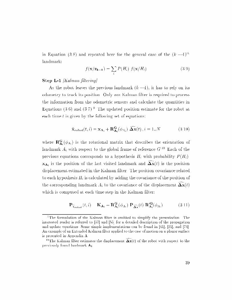
in Equation (3.8) and repeated here for the general case of the (k 1)th
landmark:
f(x=zk1) =Xi
P (Hi) f(x=Hi) (3.9)
Step L-1 [Kalman ltering]
As the robot leaves the previous landmark (k 1), it has to rely on its
odometry to track its position. Only one Kalman lter is required to process
the information from the odometric sensors and calculate the quantities in
Equations (3.6) and (3.7).9 The updated position estimate for the robot at
each time t is given by the following set of equations:
bxrobot(t; i) = xAi+RG
Ai(Ai
) dx(t) ; i = 1::N (3.10)
where RG
Ai(Ai
) is the rotational matrix that describes the orientation of
landmark Ai with respect to the global frame of reference G.10 Each of the
previous equations corresponds to a hypothesis Hi with probability P (Hi).
xAiis the position of the last visited landmark and dx(t) is the position
displacement estimated in the Kalman lter. The position covariance related
to each hypothesisHi is calculated by adding the covariance of the position of
the corresponding landmark Ai to the covariance of the displacement dx(t)which is computed at each time step in the Kalman lter:
Pbxrobot (t; i) =KAi+RG
Ai(Ai
) Pcx(t) R0GAi(Ai
) (3.11)
9The formulation of the Kalman lter is omitted to simplify the presentation. The
interested reader is referred to [57] and [55] for a detailed description of the propagation
and update equations. Some simple implementations can be found in [41], [21], and [74].
An example of an Extended Kalman lter applied to the case of motion on a planar surface
is presented in Appendix A.10The Kalman lter estimates the displacement dx(t) of the robot with respect to the
previously found landmark Ai.
39
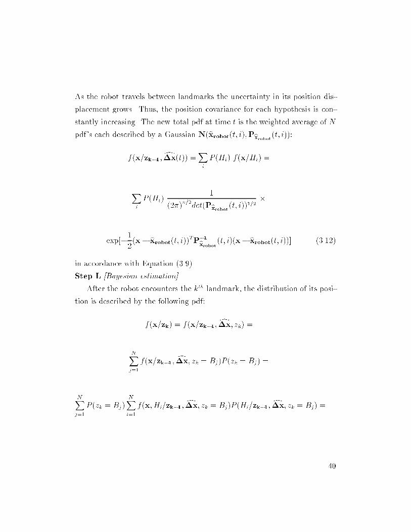
As the robot travels between landmarks the uncertainty in its position dis-
placement grows. Thus, the position covariance for each hypothesis is con-
stantly increasing. The new total pdf at time t is the weighted average of N
pdf's each described by a Gaussian N(bxrobot(t; i);Pbxrobot(t; i)):f(x=zk1;
dx(t)) =Xi
P (Hi) f(x=Hi) =
Xi
P (Hi)1
(2)n=2
det(Pbxrobot(t; i))1=2
exp[1
2(x bxrobot(t; i))TP1bxrobot (t; i)(x bxrobot(t; i))] (3.12)
in accordance with Equation (3.9).
Step L [Bayesian estimation]
After the robot encounters the kth landmark, the distribution of its posi-
tion is described by the following pdf:
f(x=zk) = f(x=zk1; dx; zk) =
NXj=1
f(x=zk1; dx; zk = Bj)P (zk = Bj) =
NXj=1
P (zk = Bj)NXi=1
f(x;Hi=zk1; dx; zk = Bj)P (Hi=zk1; dx; zk = Bj) =
40
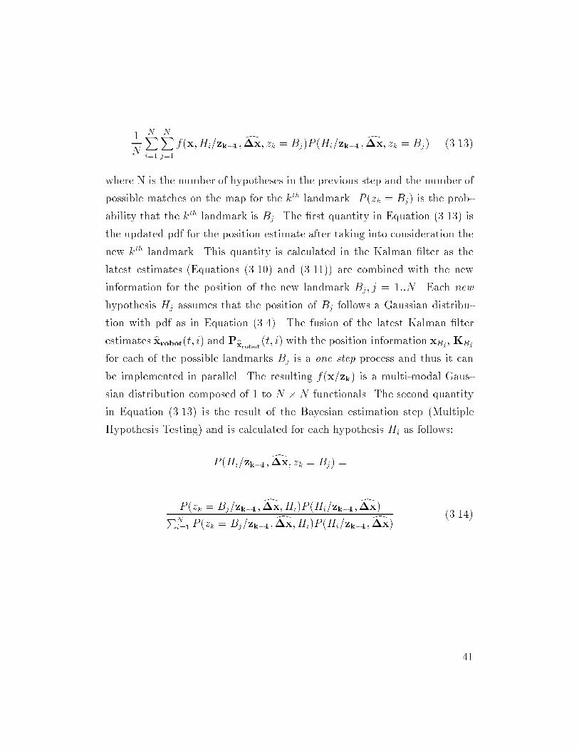
1
N
NXi=1
NXj=1
f(x;Hi=zk1; dx; zk = Bj)P (Hi=zk1; dx; zk = Bj) (3.13)
where N is the number of hypotheses in the previous step and the number of
possible matches on the map for the kth landmark. P (zk = Bj) is the prob-
ability that the kth landmark is Bj. The rst quantity in Equation (3.13) is
the updated pdf for the position estimate after taking into consideration the
new kth landmark. This quantity is calculated in the Kalman lter as the
latest estimates (Equations (3.10) and (3.11)) are combined with the new
information for the position of the new landmark Bj; j = 1::N . Each new
hypothesis Hj assumes that the position of Bj follows a Gaussian distribu-
tion with pdf as in Equation (3.4). The fusion of the latest Kalman lter
estimates bxrobot(t; i) and Pbxrobot(t; i) with the position information xBj, KBj
for each of the possible landmarks Bj is a one step process and thus it can
be implemented in parallel. The resulting f(x=zk) is a multi-modal Gaus-
sian distribution composed of 1 to N N functionals. The second quantity
in Equation (3.13) is the result of the Bayesian estimation step (Multiple
Hypothesis Testing) and is calculated for each hypothesis Hi as follows:
P (Hi=zk1; dx; zk = Bj) =
P (zk = Bj=zk1; dx;Hi)P (Hi=zk1; dx)PNi=1 P (zk = Bj=zk1; dx;Hi)P (Hi=zk1; dx) (3.14)
41
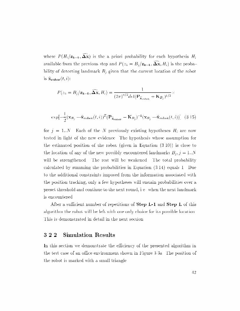
where P (Hi=zk1; dx) is the a priori probability for each hypothesis Hi
available from the previous step and P (zk = Bj=zk1; dx;Hi) is the proba-
bility of detecting landmark Bj given that the current location of the robot
is bxrobot(t; i):P (zk = Bj=zk1; dx;Hi) =
1
(2)n=2
det(Pbxrobot +KBj)1=2
exp[1
2(xBj
bxrobot(t; i))T(Pbxrobot +KBj)1(xBj
bxrobot(t; i))] (3.15)
for j = 1::N . Each of the N previously existing hypotheses Hi are now
tested in light of the new evidence. The hypothesis whose assumption for
the estimated position of the robot (given in Equation (3.10)) is close to
the location of any of the new possibly encountered landmarks Bj; j = 1::N
will be strengthened. The rest will be weakened. The total probability
calculated by summing the probabilities in Equation (3.14) equals 1. Due
to the additional constraints imposed from the information associated with
the position tracking, only a few hypotheses will sustain probabilities over a
preset threshold and continue to the next round, i.e. when the next landmark
is encountered.
After a sucient number of repetitions of Step L-1 and Step L of this
algorithm the robot will be left with one only choice for its possible location.
This is demonstrated in detail in the next section.
3.2.2 Simulation Results
In this section we demonstrate the eciency of the presented algorithm in
the test case of an oce environment shown in Figure 3.3a. The position of
the robot is marked with a small triangle.
42
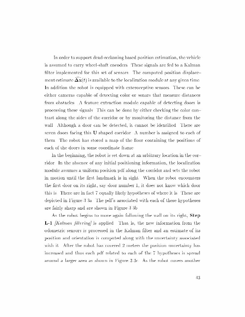
In order to support dead-reckoning based position estimation, the vehicle
is assumed to carry wheel-shaft encoders. These signals are fed to a Kalman
lter implemented for this set of sensors. The computed position displace-
ment estimate dx(t) is available to the localization module at any given time.
In addition the robot is equipped with exteroceptive sensors. These can be
either cameras capable of detecting color or sonars that measure distances
from obstacles. A feature extraction module capable of detecting doors is
processing these signals. This can be done by either checking the color con-
trast along the sides of the corridor or by monitoring the distance from the
wall. Although a door can be detected, it cannot be identied. There are
seven doors facing this U shaped corridor. A number is assigned to each of
them. The robot has stored a map of the oor containing the positions of
each of the doors in some coordinate frame.
In the beginning, the robot is set down at an arbitrary location in the cor-
ridor. In the absence of any initial positioning information, the localization
module assumes a uniform position pdf along the corridor and sets the robot
in motion until the rst landmark is in sight. When the robot encounters
the rst door on its right, say door number 1, it does not know which door
this is. There are in fact 7 equally likely hypotheses of where it is. These are
depicted in Figure 3.3a. The pdf's associated with each of these hypotheses
are fairly sharp and are shown in Figure 3.3b.
As the robot begins to move again following the wall on its right, Step
L-1 [Kalman ltering] is applied. That is, the new information from the
odometric sensors is processed in the Kalman lter and an estimate of its
position and orientation is computed along with the uncertainty associated
with it. After the robot has covered 2 meters the position uncertainty has
increased and thus each pdf related to each of the 7 hypotheses is spread
around a larger area as shown in Figure 3.3c. As the robot covers another
43
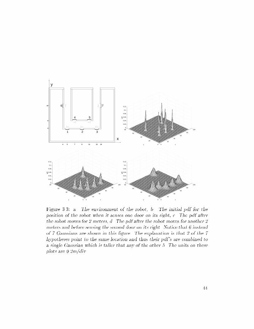
1 2 3
4 5
6 7
x
y
10
6
4
4 5 7 9 11 13 14 0
20
40
60
80
100
0
20
40
60
800
0.02
0.04
0.06
0.08
0.1
0.12
xy
0
20
40
60
80
100
0
20
40
60
800
0.02
0.04
0.06
0.08
0.1
0.12
xy
0
20
40
60
80
100
0
20
40
60
800
0.02
0.04
0.06
0.08
0.1
0.12
xy
Figure 3.3: a. The environment of the robot, b. The initial pdf for the
position of the robot when it senses one door on its right, c. The pdf after
the robot moves for 2 meters, d. The pdf after the robot moves for another 2
meters and before sensing the second door on its right. Notice that 6 instead
of 7 Gaussians are shown in this gure. The explanation is that 2 of the 7
hypotheses point to the same location and thus their pdf's are combined to
a single Gaussian which is taller that any of the other 5. The units on these
plots are 0.2m/div.
44
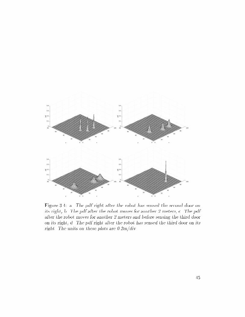
0
20
40
60
80
100
0
20
40
60
800
0.1
0.2
0.3
0.4
xy
0
20
40
60
80
100
0
20
40
60
800
0.1
0.2
0.3
0.4
xy
0
20
40
60
80
100
0
20
40
60
800
0.1
0.2
0.3
0.4
xy
0
20
40
60
80
100
0
20
40
60
800
0.2
0.4
0.6
0.8
xy
Figure 3.4: a. The pdf right after the robot has sensed the second door on
its right, b. The pdf after the robot moves for another 2 meters, c. The pdf
after the robot moves for another 2 meters and before sensing the third door
on its right, d. The pdf right after the robot has sensed the third door on its
right. The units on these plots are 0.2m/div.
45
2 meters this phenomenon becomes more prominent. This can be seen in
Figure 3.3d.
After the robot has covered a total of 4 meters, it detects another door
on its right (door number 2). Application of Step L [Bayesian estimation]
of the algorithm immediately reduces the number of hypotheses to 3. Out
of the 7 previous hypotheses only 3 are possible. These are the ones that
assumed that the previous landmark was door number 1, door number 2,
or door number 5. For these hypotheses there is a new door on the right
side of the robot after the vehicle has moved for 4 meters. In Figure 3.4a
we see again that the precise localization information related to a potential
landmark makes the pdf's for each of the surviving hypotheses sharp again.
The robot has to travel a longer distance before it is able to determine
its position uniquely. Step L-1 [Kalman ltering] is applied again and thus
the position estimates related to the 3 hypotheses deteriorate. As the robot
moves for another 2 + 2 meters, the uncertainty increase is shown in Fig-
ures 3.4b and 3.4c. Finally, the robot senses a third door on its right (door
number 3) and by applying Step L [Bayesian estimation] of the algorithm
again, it concludes with the position estimate described by the pdf of Figure
3.4d.
3.2.3 Environments with many types of features
In this section we extend the Multiple Hypothesis Tracking approach to the
localization problem when more than one feature type is considered. In
addition to doors, interior and exterior corners can also be used as dierent
types of potential landmarks for localization in indoor environments. The
following formulation shows that the proposed approach builds naturally on
the methodology introduced in Section 3.2.1. The suggested algorithm is
similar to the algorithm presented in Figure 3.2. The main dierence in
46
the treatment of this case and the case of only one type of feature is that
Equation (3.13) has to be modied in order to accommodate the existence
of dierent types of features. After the robot encounters the kth landmark,
the distribution of its position is described by the following pdf:
f(x=zk) = f(x=zk1;dx; zk) =
MXj=1
f(x=zk1; dx; zk = Bj)P (zk = Bj=Type(zk) = B)P (Type(zk) = B) =
MXj=1
P (zk = Bj=Type(zk) = B)P (Type(zk) = B)
NXi=1
f(x;Hi=zk1; dx; zk = Bj)P (Hi=zk1; dx; zk = Bj) =
NXi=1
MXj=1
P (zk = Bj=Type(zk) = B)P (Type(zk) = B)
f(x;Hi=zk1; dx; zk = Bj)P (Hi=zk1; dx; zk = Bj) (3.16)
where N is the number of hypotheses in the previous step and the M is the
number of possible matches on the map for the kth landmark. P (zk = Bj) is
the probability that the kth landmark is Bj and is calculated as the product
of P (zk = Bj=Type(zk) = B) which is the probability that the landmark in
47
sight is Bj given that its type is B, and P (Type(zk) = B) which is the prob-
ability that the feature type is B. This last probability is provided by the
feature extraction module. We assume that the feature extraction module
can detect landmarks of dierent types and provide the level of condence
associated with the decision about the type.
The quantity f(x;Hi=zk1; dx; zk = Bj) in Equation (3.16) is the up-
dated pdf for the position estimate after taking into consideration the new
kth landmark. This quantity is calculated in the Kalman lter as the latest
estimates are combined with the new information for the position of the new
landmark Bj . Each new hypothesis Hj assumes that the position of Bj fol-
lows a Gaussian distribution with pdf as in Equation (3.4). The fusion of the
latest Kalman lter estimates bxrobot(t; i) and Pbxrobot (t; i) with the position
information xBj, KBj
for each of the possible landmarks Bj is a one step
process and thus it can be implemented in parallel. The resulting f(x=zk) is
a multi-modal Gaussian distribution composed of 1 to N M functionals.
The quantity P (Hi=zk1; dx; zk = Bj) in Equation (3.16) is the result of the
Bayesian estimation step (Multiple Hypothesis Testing) and is calculated for
each hypothesis Hi using Equations (3.14) and (3.15).
3.2.4 Experimental Results
In order to validate theMultiple Hypothesis Tracking approach within areas11
with dierent types of features, we implemented this algorithm and tested it
for the case of a Pioneer 2 mobile robot equipped with wheel-shaft encoders
and a SICK LMS 200 laser scanner.
The Pioneer 2 mobile robot manufactured by ActivMedia shown in Fig-
ure 3.5 has 2 active wheels in the front and 1 passive caster in the rear. The
11All the experiments presented here were conducted on the second oor of the Henry
Salvatori Computer Science Center on the USC campus.
48
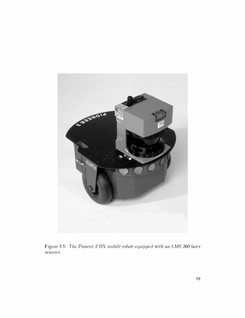
Figure 3.5: The Pioneer 2 DX mobile robot equipped with an LMS 200 laser
scanner.
49
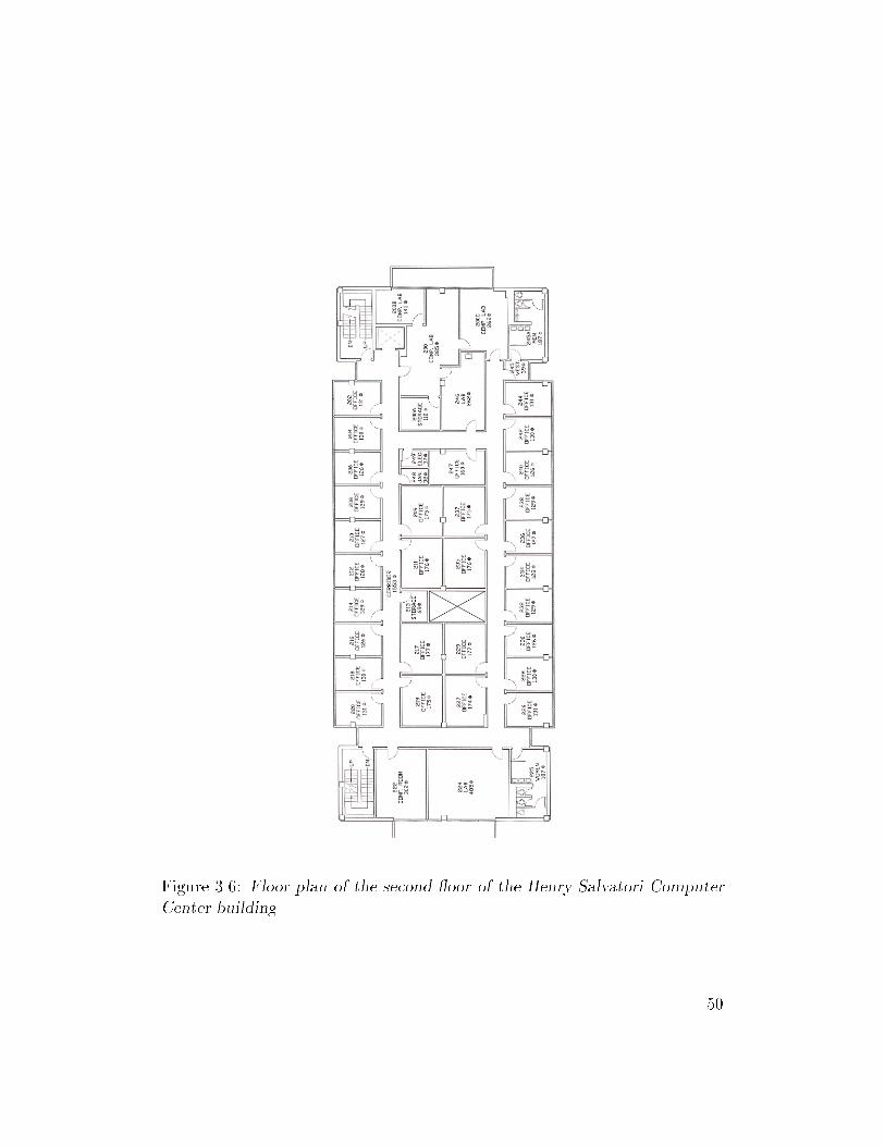
Figure 3.6: Floor plan of the second oor of the Henry Salvatori Computer
Center building.
50
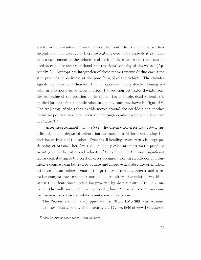
2 wheel-shaft encoders are mounted on the front wheels and measure their
revolutions. The average of these revolutions every 0:05 seconds is available
as a measurement of the velocities of each of these two wheels and can be
used to calculate the transitional and rotational velocity of the vehicle (Ap-
pendix A). Appropriate integration of these measurements during each time
step provides an estimate of the pose [x; y; ] of the vehicle. The encoder
signals are noisy and therefore their integration during dead-reckoning re-
sults in odometric error accumulation; the position estimates deviate from
the real value of the position of the robot. For example, dead-reckoning is
applied for localizing a mobile robot in the environment shown in Figure 3.6.
The trajectory of the robot as this moves around the corridors and reaches
its initial position has been calculated through dead-reckoning and is shown
in Figure 3.7.
After approximately 40 meters, the orientation error has grown sig-
nicantly. This degraded orientation estimate is used for propagating the
position estimate of the robot. Even small heading errors result in large po-
sitioning errors and therefore the low quality orientation estimates provided
by integrating the rotational velocity of the vehicle are the most signicant
factor contributing to the position error accumulation. In an outdoor environ-
ment a compass can be used to update and improve this absolute orientation
estimate. In an indoor scenario, the presence of metallic objects and wires
makes compass measurements unreliable. An alternative solution would be
to use the orientation information provided by the structure of the environ-
ment. The walls around the robot usually have 2 possible orientations and
can be used to extract absolute orientation information.
The Pioneer 2 robot is equipped with an SICK LMS 300 laser scanner.
This sensor12 has accuracy of approximately 15mm, eld of view 180 degrees
12Also known as laser radar, lidar or ladar.
51
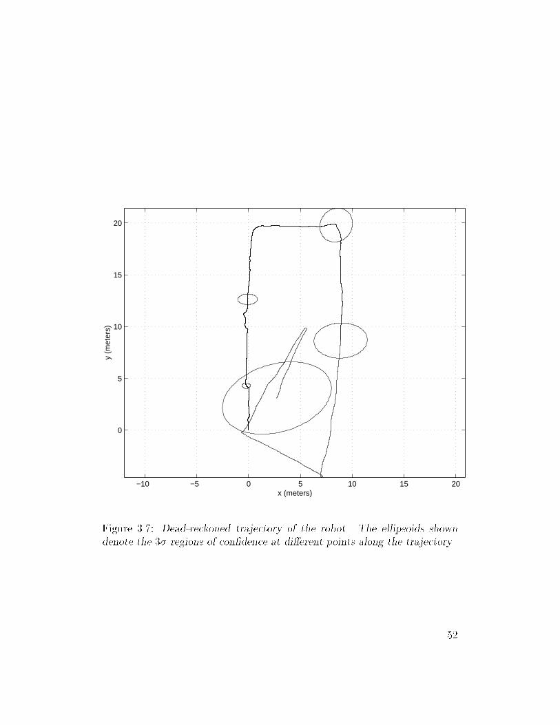
−10 −5 0 5 10 15 20
0
5
10
15
20
y (m
eter
s)
x (meters)
Figure 3.7: Dead-reckoned trajectory of the robot. The ellipsoids shown
denote the 3 regions of condence at dierent points along the trajectory.
52
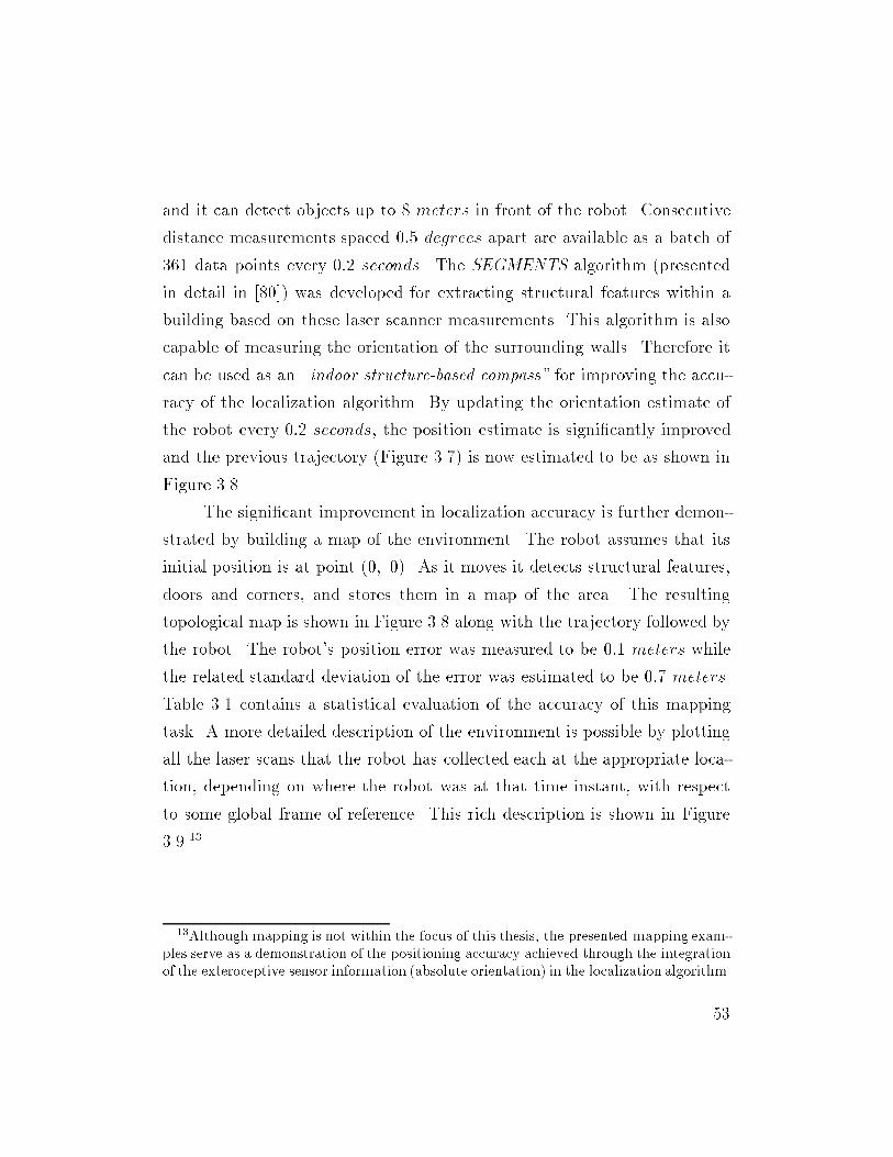
and it can detect objects up to 8 meters in front of the robot. Consecutive
distance measurements spaced 0:5 degrees apart are available as a batch of
361 data points every 0:2 seconds. The SEGMENTS algorithm (presented
in detail in [80]) was developed for extracting structural features within a
building based on these laser scanner measurements. This algorithm is also
capable of measuring the orientation of the surrounding walls. Therefore it
can be used as an \indoor structure-based compass" for improving the accu-
racy of the localization algorithm. By updating the orientation estimate of
the robot every 0:2 seconds, the position estimate is signicantly improved
and the previous trajectory (Figure 3.7) is now estimated to be as shown in
Figure 3.8.
The signicant improvement in localization accuracy is further demon-
strated by building a map of the environment. The robot assumes that its
initial position is at point (0; 0). As it moves it detects structural features,
doors and corners, and stores them in a map of the area. The resulting
topological map is shown in Figure 3.8 along with the trajectory followed by
the robot. The robot's position error was measured to be 0:1 meters while
the related standard deviation of the error was estimated to be 0:7 meters.
Table 3.1 contains a statistical evaluation of the accuracy of this mapping
task. A more detailed description of the environment is possible by plotting
all the laser scans that the robot has collected each at the appropriate loca-
tion, depending on where the robot was at that time instant, with respect
to some global frame of reference. This rich description is shown in Figure
3.9.13
13Although mapping is not within the focus of this thesis, the presented mapping exam-
ples serve as a demonstration of the positioning accuracy achieved through the integration
of the exteroceptive sensor information (absolute orientation) in the localization algorithm.
53
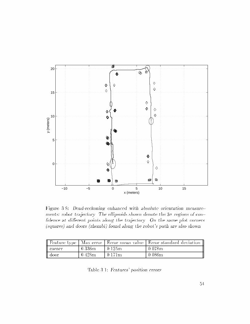
−10 −5 0 5 10 15
0
5
10
15
20
x (meters)
y (m
eter
s)
Figure 3.8: Dead-reckoning enhanced with absolute orientation measure-
ments: robot trajectory. The ellipsoids shown denote the 3 regions of con-
dence at dierent points along the trajectory. On the same plot corners
(squares) and doors (rhombi) found along the robot's path are also shown.
Feature type Max error Error mean value Error standard deviation
corner 0.336m 0.125m 0.078m
door 0.428m 0.171m 0.086m
Table 3.1: Features' position errors.
54
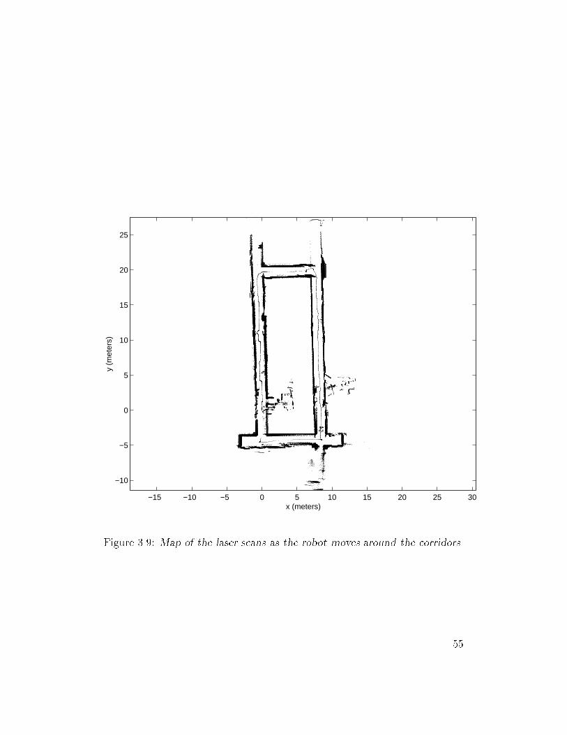
−15 −10 −5 0 5 10 15 20 25 30
−10
−5
0
5
10
15
20
25
x (meters)
y (m
eter
s)
Figure 3.9: Map of the laser scans as the robot moves around the corridors.
55
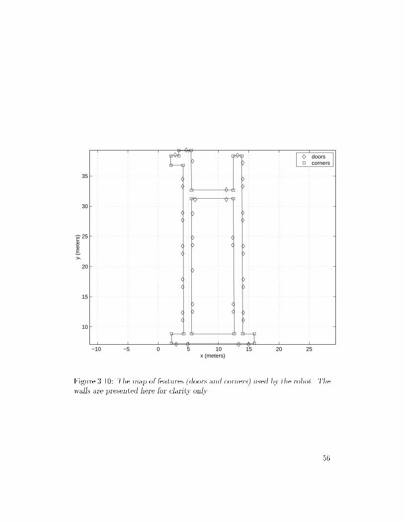
−10 −5 0 5 10 15 20 25
10
15
20
25
30
35
x (meters)
y (m
eter
s)
doors corners
Figure 3.10: The map of features (doors and corners) used by the robot. The
walls are presented here for clarity only.
56
At this point we present an experimental validation of the theoretical
results presented in Section 3.2.3. We describe two example cases where
the Multiple Hypothesis Tracking algorithm was applied in order to glob-
ally localize a mobile robot with unknown initial position. This situation is
usually referred to as the \kidnapped robot" problem and it is probably the
most dicult task in robot navigation. During each of the following cases a
dierent starting point was selected. The robot equipped with a topological
description of the environment (portrayed as a map in Figure 3.10) must nd
the unique location on the map that corresponds to its true position. Only
one Kalman lter is being used for tracking its displacement.
Scenario 1: The rst landmark seen by the robot is a door on
its left (oce 216 in Figure 3.6). Therefore, for this particular environment
the initial number of hypotheses is 42. These 42 hypotheses are depicted in
Figure 3.11 as ellipsoids14 each of them marking the 3 region of condence
of the corresponding hypothesis. The respective orientation of the robot at
each of these locations is also shown (small line originating from the center of
each ellipsoid). After a few steps the robot detects another door (oce 214)
on its left and based on the distance from the previous feature, it reduces
the number of hypotheses to 15 (Figure 3.12). Almost immediately after
that the appearance of the rst door on its right (room 213) allows only 5
hypotheses to continue to the next stage (Figure 3.13). Moving along the
corridor and nding a second pair of doors on its left (oces 212 and 210)
the total number of hypotheses decreases to 4 (Figure 3.14) and 3 (Figure
3.15) respectively. The appearance of another door on its right (oce 211)
14The feature extraction module determines the position of each door detected with
respect to the robot with higher uncertainty along the axis parallel to the length of the
door. Therefore the 3 regions of condence are ellipsoids instead of circles.
57
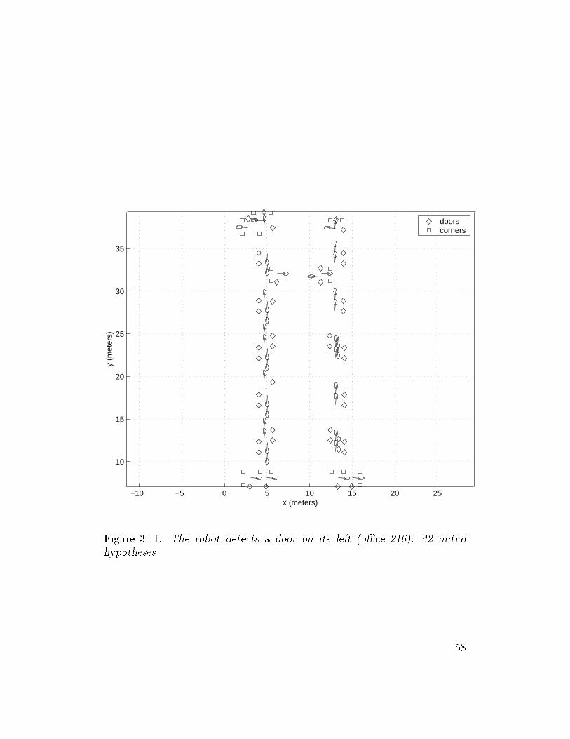
−10 −5 0 5 10 15 20 25
10
15
20
25
30
35
x (meters)
y (m
eter
s)
doors corners
Figure 3.11: The robot detects a door on its left (oce 216): 42 initial
hypotheses.
58
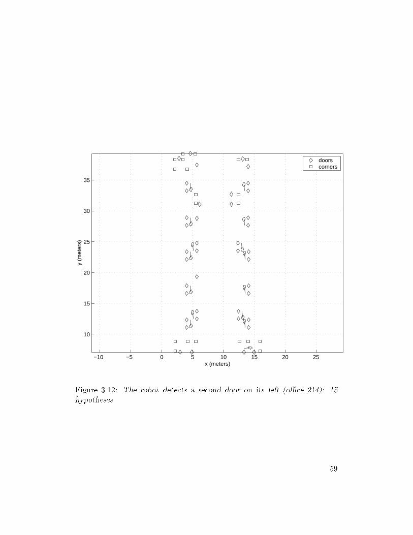
−10 −5 0 5 10 15 20 25
10
15
20
25
30
35
x (meters)
y (m
eter
s)
doors corners
Figure 3.12: The robot detects a second door on its left (oce 214): 15
hypotheses.
59
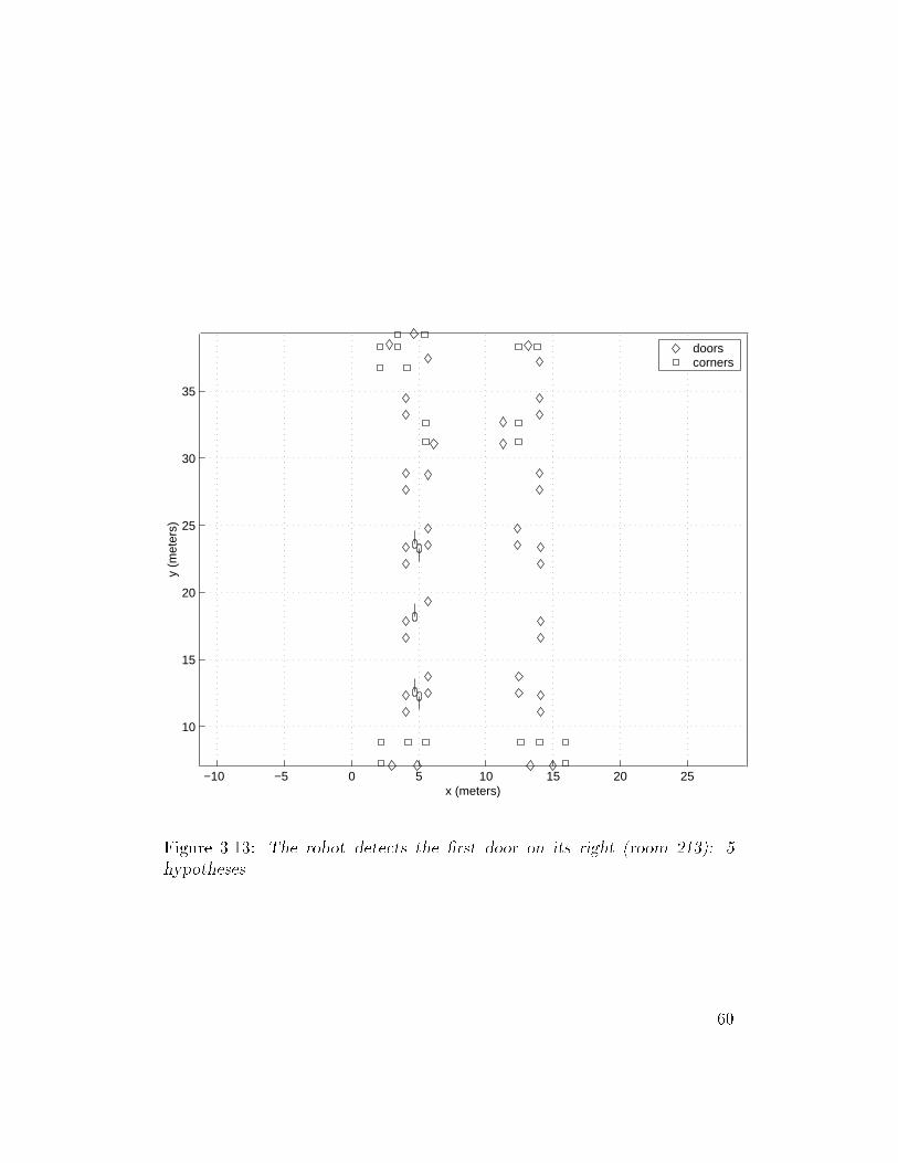
−10 −5 0 5 10 15 20 25
10
15
20
25
30
35
x (meters)
y (m
eter
s)
doors corners
Figure 3.13: The robot detects the rst door on its right (room 213): 5
hypotheses.
60
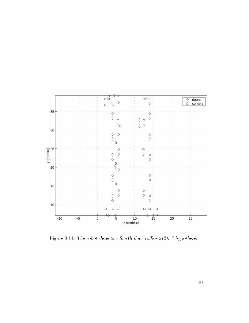
−10 −5 0 5 10 15 20 25
10
15
20
25
30
35
x (meters)
y (m
eter
s)
doors corners
Figure 3.14: The robot detects a fourth door (oce 212): 4 hypotheses.
61
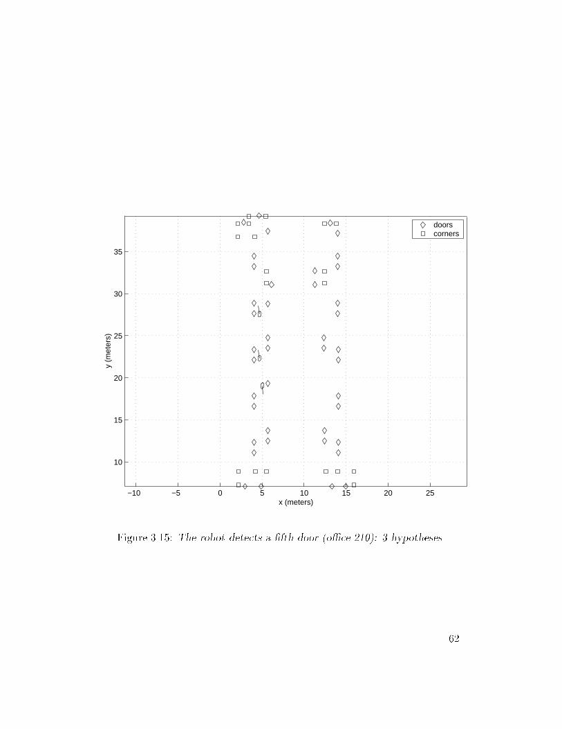
−10 −5 0 5 10 15 20 25
10
15
20
25
30
35
x (meters)
y (m
eter
s)
doors corners
Figure 3.15: The robot detects a fth door (oce 210): 3 hypotheses.
62

−10 −5 0 5 10 15 20 25
10
15
20
25
30
35
x (meters)
y (m
eter
s)
doors corners
Figure 3.16: The robot detects a sixth door (oce 211): 2 hypotheses.
63
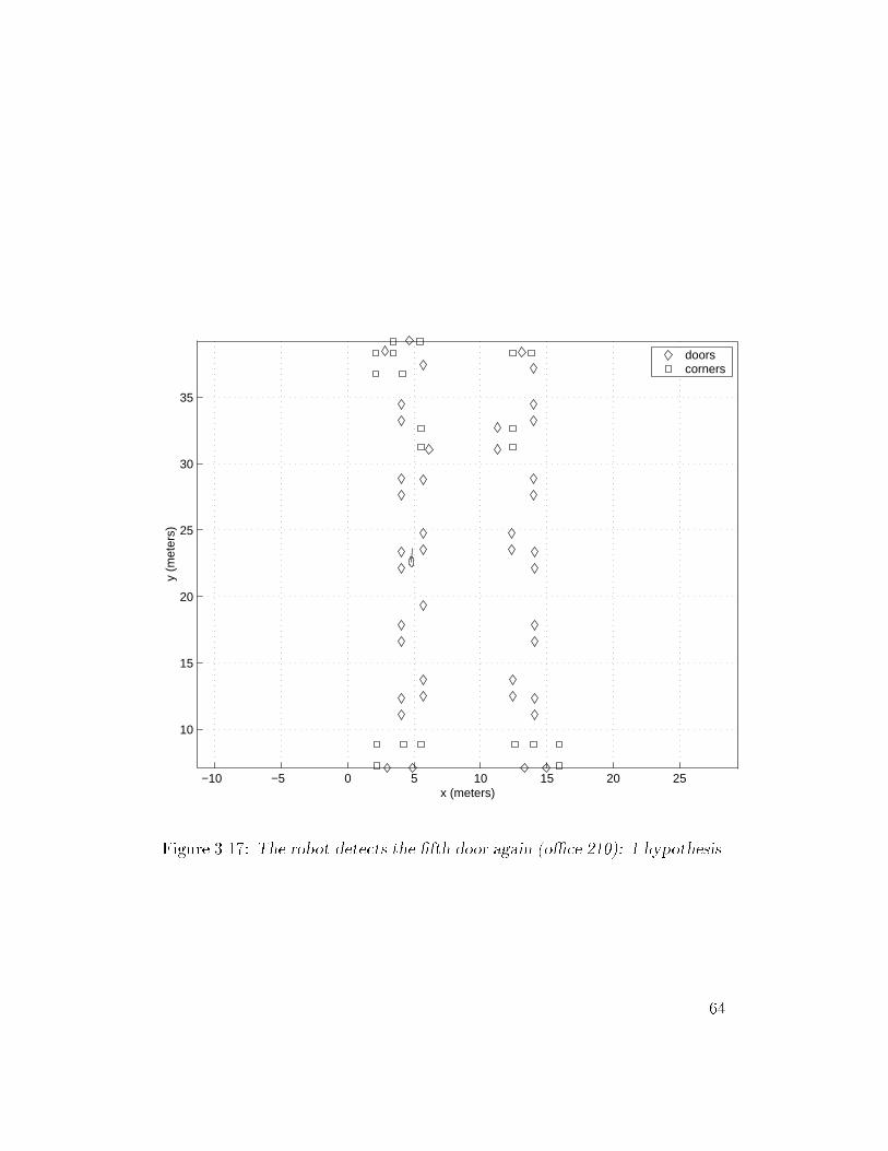
−10 −5 0 5 10 15 20 25
10
15
20
25
30
35
x (meters)
y (m
eter
s)
doors corners
Figure 3.17: The robot detects the fth door again (oce 210): 1 hypothesis.
64
terminates one more hypothesis (Figure 3.16) while a more careful measure-
ment of the relative distance of the last two doors leaves the robot with a
single hypothesis regarding its position (Figure 3.17).
Scenario 2: In this case the rst landmark seen by the robot is a corner,
the one across room 249. Now the initial number of hypotheses is 20. These
20 hypotheses are depicted in Figure 3.18 as circles15 each of them marking
the 3 region of condence of the corresponding hypothesis. The respective
orientation of the robot at each of these locations is also shown (small line
originating from the center of each circle). As the robot moves and detects
the rst door on its right (room 249), the number of hypotheses is imme-
diately reduced to 7 (Figure 3.19). Approximately 5 meters later it nds
another door on its left (lab 246) and that reduces the number of hypotheses
to 2 (Figure 3.20). Finally, the detection of a second door on its right (oce
247) resolves the ambiguity between the two last candidate hypotheses and
allows the robot to globally localize itself (Figure 3.21).
The Multiple Hypotheses Tracking algorithm was tested for 29 dierent
initial locations within the mapped area. During the exploration phase, the
robot searches for features of the environment in order to determine the ini-
tial 42 or 20 (depending on the type of the rst feature in view) hypotheses
regarding its position. As the robot encounters more features it validates the
previous set of hypotheses in view of the new possible ones. The odometric
information collected inbetween two consecutive landmarks is being used for
updating the probabilities for each of the previous hypotheses. A very small
probability value16 signals termination of the corresponding hypothesis.
15The feature extraction module determines the position of each detected corner with
respect to the robot with the same uncertainty along both axes. Therefore, in this case
the 3 regions of condence are circles.16If a door is detected the threshold for accepting a hypothesis as valid is set to be
0:5 (1=42). When a corner is detected the cut o value is set to be 0:5 (1=20).
65
After the robot has explored a sucient portion of the environment
so as to terminate all but one of the initial hypotheses, it is considered to
be globally localized. Its position is described by one only hypothesis with
probability 1. Thereafter, the robot has to track its position while periodi-
cally updating it with information provided by new landmarks found along
its way. Landmark identication is not an issue any more since the robot
knows its position in global coordinates and it can use this information to
match the encountered landmark with its closest neighbor in the (global)
map of the area.
Every time the robot sees a new landmark along its trajectory and uses
it to update its position estimate, there are 2 types of errors related to this
update: (1) the odometric error accumulated since the last landmark seen
by the robot, and (2) the error due to laser scanner noise and precision that
degrades the accuracy of the feature extraction module. Appropriate fusion
of these two sources of position information using a Kalman lter provides
the optimal (in the minimum mean-square error sense) estimate for the po-
sition of the robot. The remaining trajectory of the robot after it has been
globally localized (Figure 3.17) is shown in Figure 3.22 while the associated
uncertainties are portrayed in Figure 3.23.
3.2.5 Extensions
In this Chapter we investigated the reduction of the localization uncertainty
due to the appearance of features. Here we investigate the eect of a fea-
ture missing from the location where is expected. We extend the Multiple
Hypothesis Tracking framework in order to exploit this additional source of
information.
66
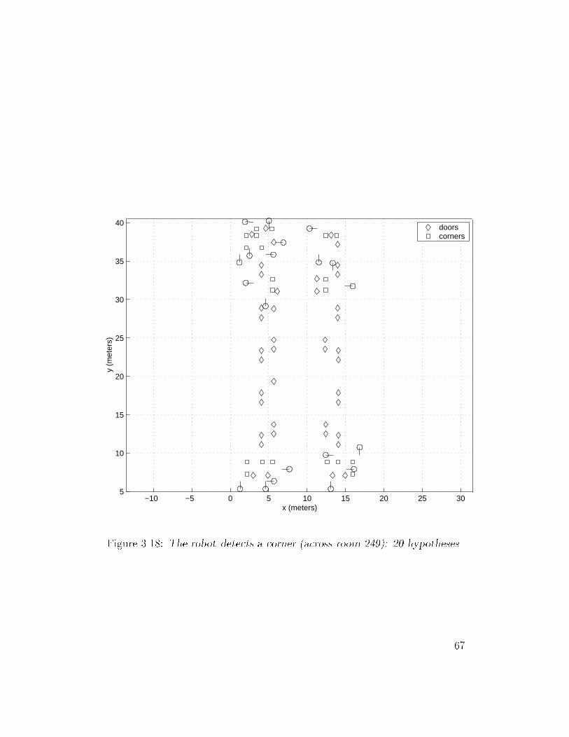
−10 −5 0 5 10 15 20 25 305
10
15
20
25
30
35
40
x (meters)
y (m
eter
s)
doors corners
Figure 3.18: The robot detects a corner (across room 249): 20 hypotheses.
67
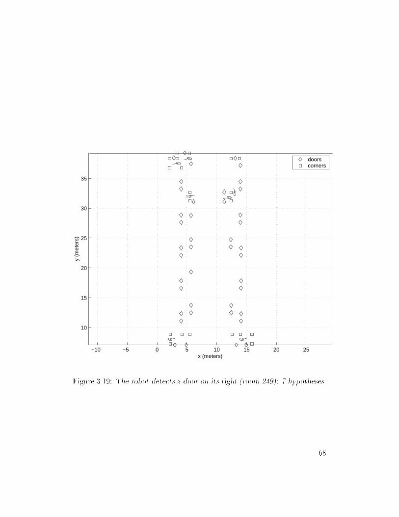
−10 −5 0 5 10 15 20 25
10
15
20
25
30
35
x (meters)
y (m
eter
s)
doors corners
Figure 3.19: The robot detects a door on its right (room 249): 7 hypotheses.
68
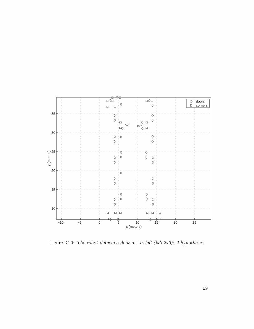
−10 −5 0 5 10 15 20 25
10
15
20
25
30
35
x (meters)
y (m
eter
s)
doors corners
Figure 3.20: The robot detects a door on its left (lab 246): 2 hypotheses.
69
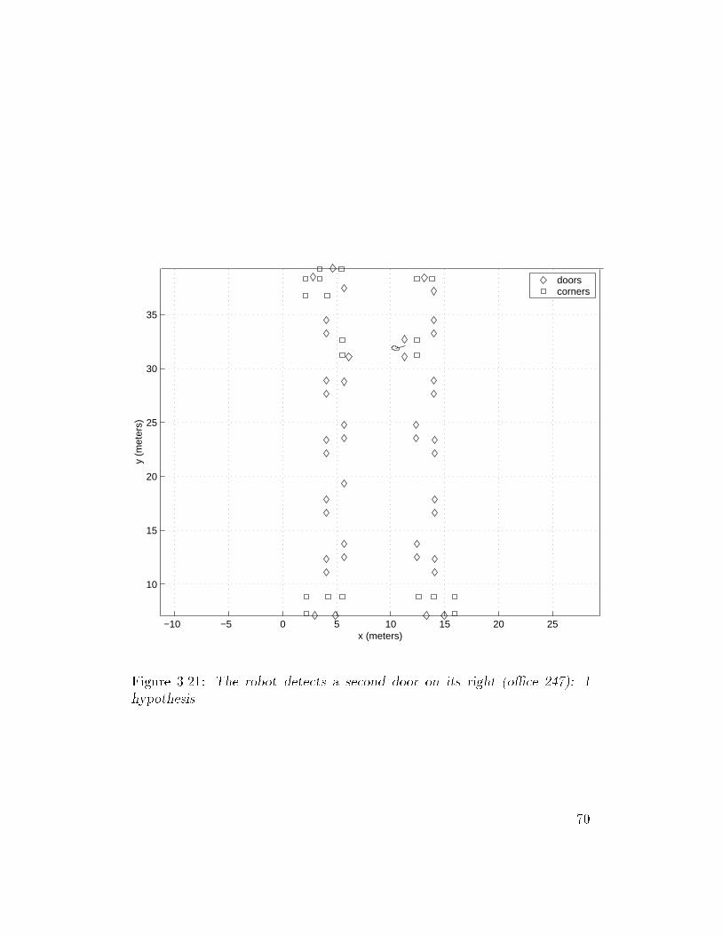
−10 −5 0 5 10 15 20 25
10
15
20
25
30
35
x (meters)
y (m
eter
s)
doors corners
Figure 3.21: The robot detects a second door on its right (oce 247): 1
hypothesis.
70
The algorithm described here is the one shown in Figure 3.24. There
is an extra step added to this when compared to the algorithm presented
in Figure 3.2. At every time instant, along with the position tracking, the
localization module checks for the existence of features in the environment.
Thus, the competition between the hypotheses continues even when there is
no landmark in sight. The absence of a landmark carries enough information
to terminate some of the hypotheses and thus strengthen others (the total
probability of all the hypotheses adds up to one at any given time). By
detecting what is not in its vicinity, the robot can prune the number of
existing hypotheses.
The following formulation shows that this approach is an extension of the
methodology introduced in Section 3.2.1. Starting from Equation (3.13) the
distribution of the position of the robot is described by the following pdf:
f(x=zk) = f(x=zk1; dx; zk = ) =
NXi=1
f(x;Hi=zk1; dx; zk = )P (Hi=zk1; dx; zk = ) =
NXi=1
f(x;Hi=zk1; dx)P (Hi=zk1; dx; zk = ) (3.17)
where N is the number of hypotheses in the previous step. zk = denotes
that there is no feature detected at this time instant. The rst quantity in
Equation (3.17) is the current pdf for the position estimate which is indepen-
dent of the absence of a landmark. This quantity is updated by the Kalman
lter continuously by adding the latest Kalman lter estimates dx(t) and
71
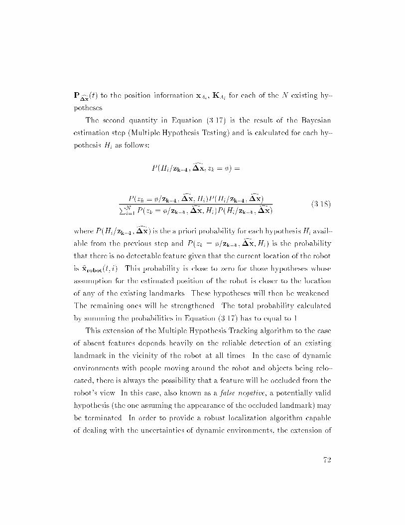
Pcx(t) to the position information xAi, KAi
for each of the N existing hy-
potheses.
The second quantity in Equation (3.17) is the result of the Bayesian
estimation step (Multiple Hypothesis Testing) and is calculated for each hy-
pothesis Hi as follows:
P (Hi=zk1; dx; zk = ) =
P (zk = =zk1; dx;Hi)P (Hi=zk1; dx)PNi=1 P (zk = =zk1; dx;Hi)P (Hi=zk1; dx) (3.18)
where P (Hi=zk1; dx) is the a priori probability for each hypothesisHi avail-
able from the previous step and P (zk = =zk1; dx;Hi) is the probability
that there is no detectable feature given that the current location of the robot
is bxrobot(t; i). This probability is close to zero for those hypotheses whose
assumption for the estimated position of the robot is closer to the location
of any of the existing landmarks. These hypotheses will then be weakened.
The remaining ones will be strengthened. The total probability calculated
by summing the probabilities in Equation (3.17) has to equal to 1.
This extension of the Multiple Hypothesis Tracking algorithm to the case
of absent features depends heavily on the reliable detection of an existing
landmark in the vicinity of the robot at all times. In the case of dynamic
environments with people moving around the robot and objects being relo-
cated, there is always the possibility that a feature will be occluded from the
robot's view. In this case, also known as a false negative, a potentially valid
hypothesis (the one assuming the appearance of the occluded landmark) may
be terminated. In order to provide a robust localization algorithm capable
of dealing with the uncertainties of dynamic environments, the extension of
72

the Multiple Hypothesis Tracking algorithm to the case of absent features
was not included in the implementation used for the experiments presented
in the previous section.
73
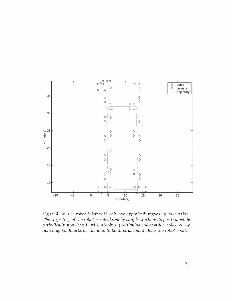
−10 −5 0 5 10 15 20 25
10
15
20
25
30
35
x (meters)
y (m
eter
s)
doors corners trajectory
Figure 3.22: The robot is left with only one hypothesis regarding its location.
The trajectory of the robot is calculated by simply tracking its position while
periodically updating it with absolute positioning information collected by
matching landmarks on the map to landmarks found along the robot's path.
74
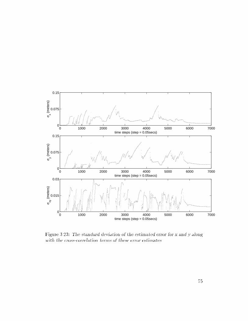
0 1000 2000 3000 4000 5000 6000 70000
0.075
0.15
σ x (m
eter
s)
time steps (step = 0.05secs)
0 1000 2000 3000 4000 5000 6000 70000
0.075
0.15
σ y (m
eter
s)
time steps (step = 0.05secs)
0 1000 2000 3000 4000 5000 6000 70000
0.015
0.03
σ xy (
met
ers)
time steps (step = 0.05secs)
Figure 3.23: The standard deviation of the estimated error for x and y along
with the cross-correlation terms of these error estimates.
75
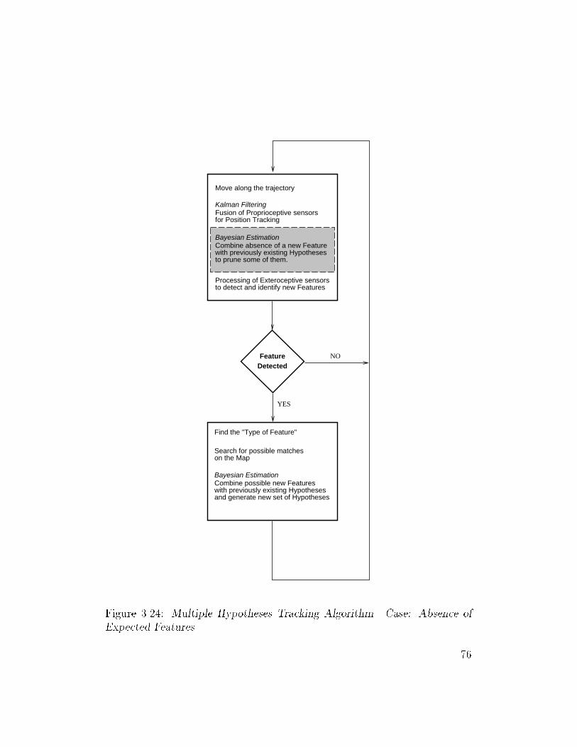
FeatureDetected
Combine possible new Featureswith previously existing Hypothesesand generate new set of Hypotheses
Bayesian Estimation
Find the "Type of Feature"
Search for possible matcheson the Map
YES
NO
Kalman FilteringFusion of Proprioceptive sensorsfor Position Tracking
Move along the trajectory
Processing of Exteroceptive sensorsto detect and identify new Features
Combine absence of a new Featurewith previously existing Hypothesesto prune some of them.
Bayesian Estimation
Figure 3.24: Multiple Hypotheses Tracking Algorithm. Case: Absence of
Expected Features.
76
Chapter 4
Smoother Based Attitude Estimation 2-D
4.1 Introduction
In this Chapter we concentrate on the problem of mobile robot localiza-
tion when absolute measurements are available only intermittently. During
a mapping task for example, a robot is necessary to know its precise location
at all times. If GPS signals are used for determining the position of the
robot, there is always the probability that these will not be available, espe-
cially in the vicinity of tall buildings or structures. When the GPS signals
are occluded the robot would have to rely on its odometry for propagating
its position estimates. During these intervals the reduced accuracy of the lo-
calization estimates will aect the quality of the mapping task. A new GPS
measurement will bring the positioning accuracy to a sucient level again
but it will not have any eect on any of the previous estimates. This case calls
for a new estimation scheme within which this new absolute measurement
could be used in order to increase the accuracy of the previous odometric
estimates and therefore improve the overall accuracy of the mapping task.
Here we focus on a similar problem encountered during localization on the
surface of Mars where absolute orientation measurements are only available
77
during certain time instants. The analysis presented in this and the following
chapter is tailored to the case of Rocky 7, an experimental Mars exploration
rover currently under development at the NASA Jet Propulsion Laboratory.
4.1.1 Localization and Attitude estimation
The sensor suite of Rocky 7 includes wheel encoders, gyros, accelerometers
and a sun sensor. Since there is no device measuring the absolute position
of the rover (GPS signals are not currently available on the surface of Mars),
the position can be estimated through the integration of the accelerometer
signal and/or the signals from the encoders. The quality of this estimate de-
pends heavily on the noise prole of the inertial and the odometric sensors.
Bias and noise in the accelerometer signal and imprecise encoders can cause
serious drift of the position estimate. The localization task is even more
dicult because the propagation of the position relies upon the attitude es-
timate. Even small errors in the orientation can rapidly become large errors
in position. Formally speaking, the position is not observable and thus the
uncertainty of the position estimate will grow without bounds. The most
promising course of action with the current set of sensors would be to focus
on gaining a very precise attitude estimate. As a result the position uncer-
tainty will grow at a slower rate and will allow for increased autonomy. The
estimator will maintain accurate position estimates during longer traverses
before other localization techniques (such as visual tracking) are required.
The attitude estimate is used twice during position estimation:
i) The accelerometer measures both the vehicle's acceleration and the
projection of the gravitational acceleration on the accelerometer local frame.
The relation between these is described by the following equation:
~p(t) = ~f(t)=m = ~aaccelerometer(t)A(q(t))~g (4.1)
78
where ~p is the vehicle's (non-gravitational) acceleration, ~aaccelerometer is the
measurement from the 3-axis accelerometer and ~g is the gravitational accel-
eration. Precise knowledge of the orientation matrix A(q) is mandatory to
extract ~p accurately.
ii) The next step requires integration of ~p to derive the position. The in-
formation in ~p is local (i.e. expressed in the local coordinate frame attached
to the mobile platform) and in order to calculate the position in global co-
ordinates the attitude information is once again required:
~p(t) =Z t
0dt0
Z t0
0A(q(t00))~p(t00)dt00 (4.2)
4.1.1.1 Attitude Measuring Devices
Amongst the sensors on-board the rover, the gyroscopes can be used to cal-
culate the attitude of the vehicle by simply integrating their output signal
(the angular rate). On the other hand, the sun sensor measures directly the
values of the two components of a two-dimensional vector. This vector is the
projection of the unit vector towards the sun on the sun sensor plane. An-
other sensory input of the same nature is required in order to satisfy attitude
observability requirements. It is evident from Equations (4.1) and (4.2) that
the accelerometer is used to advance the position estimate. It can also be
used in an alternative way. An accelerometer can measure the gravitational
acceleration, a three-dimensional vector parallel to the local vertical. This
provides another orientation x independent from the sun and thus makes
the vehicle's attitude observable.
This method fails when the rover is in motion. The gravity vector is then
\contaminated" by the non-gravitational acceleration of the vehicle seen in
Equation (4.1). The gravity vector could be extracted while the vehicle is
moving if an independent measurement of its own acceleration was available.
79
Research eorts have tried to address this problem. In [93], the authors
attempt to remove the non-gravitational acceleration by approximating it.
Odometry information from the encoders is used in this approximation. Each
encoder signal has to undergo two dierentiations to provide acceleration es-
timates along the local x and y directions. The main claim reported is that
in the long term, the roll and pitch estimates from the accelerometers have
good mean values while in the short term the gyroscopes are mostly respon-
sible for the attitude estimation. It is also clear that instantaneous attitude
estimates provided by the accelerometer can be completely wrong. As the
authors mention, robot vibrations are wrongfully converted into angles and
numerical dierentiations aect the quality of the result. In their work, a
Kalman lter estimates the drift of the gyroscopes based on the accelerom-
eter information. The algorithm was tested in the case of a mobile robot
that moves on at ground except when one of the wheels climbs over a 2 cm
plank using a small inclined plane. After that the robot again moves on at
ground. We believe that this approach is sucient for indoor applications
and can deal with cases of motion over small objects but it is not accurate
enough for outdoor environments, mainly because of the limited accuracy of
the estimates of the non-gravitational acceleration. This is due to numerical
dierentiation (which amplies noise), limited precision of encoders, longitu-
dinal wheel slippage and lateral skidding during turning. The approach of
Fuke and Krotkov [28] is similar. They concentrate on motion in a straight
line over inclined surfaces (sandy craters). Their method suers from the
same drawbacks as the previously discussed method.
A more thorough consideration of the problem would require dynamic
modeling of the vehicle. An estimator that incorporates a dynamic model of
the vehicle could estimate its non-gravitational accelerations. An example
of an eort along these lines comes from the Aerobots domain. In [82], an
80
estimator for a telerobotic balloon is described. While the balloon is oating
in the air, the \swaying" of its gondola can be modeled as a pendulum. That
allows for modeling of its dynamics. The result is an estimator that, in eect,
uses the accelerometer as another source of attitude information.
4.1.1.2 Dynamic Model Replacement
In our approach we avoid dynamic modeling and we restrict ourselves to us-
ing the accelerometer only when the rover is stopped. The reasoning behind
this is as follows:
i) The most elementary reason is that every time there is a modication
of the rover (i.e. a mass changes, or a part is relocated, or dimensions are
altered) the dynamic modeling has to be redone. The produced estimator is
tailored for a specic structure. A slightly dierent vehicle would require a
new estimator.
ii) A more practical reason is that dynamic modeling would require a
very large number of states; consider that the Rocky 7 vehicle which is fairly
typical for a NASAMars rover design, has 6 wheels, 2 steering joints, 3 bogey
joints. An estimator has to be practical as far as its computational needs
are concerned. The size of the estimated state can have large computational
demands with very little gain in precision.
iii) Dynamic modeling and the added complexity caused do not always
produce the expected results. One example is an attempt by Leerts and
Markley [49] to model the attitude dynamics of the NIMBUS-6 spacecraft,
which indicated that dynamic modeling with elaborate torque models could
still not give acceptable attitude determination accuracy. For this reason
most attitude estimation applications in the aerospace domain use gyros in
a dynamic model replacement mode [95].
81
iv) Modeling a mobile robot moving on rough terrain is more complicated
than that of a spacecraft because of the interaction between the wheeled ve-
hicle and the ground.1 The external forces on a spacecraft traveling on a
ballistic trajectory in space, are precisely described by the law of gravita-
tional forces. The interaction of a rover with the ground depends on many
parameters which are dicult to measure and requires simplifying assump-
tions to be made (the point contact assumption is frequently used). The
modeling of the vehicle-terrain dynamic eects such as wheel impact, wheel
slippage, and wheel sinkage, all require prior knowledge of the ground param-
eters (i.e. friction coecients as a function of wheel slippage ratio, soil shear
strength, elastic modulus, etc). In addition, lateral slippage is not observable
and can not easily be accounted for in the dynamic model. Precise modeling
of the motors is also required to obtain the real values of the torques acting
on each of the wheels. At this point we also have to mention that the appli-
cability of Kalman ltering techniques rests on the availability of an accurate
dynamic model. An inaccurate model can cause the estimate to drift away
from the real value.
v) Looking at the problem from another perspective, the vehicle has a
suspension system (bogey joints) that allows it to climb rocks 1.5 times its
wheel diameter [39]. One of the purposes of every suspension system is to
decouple the vehicle's motion from the terrain morphology (Figure 4.1). The
\ideal" suspension system would support a motion of the vehicle that would
imitate to some extent, the motion of a hovercraft. The rover then could
move in a very smooth fashion. A motion like this is prone to be eectively
1Another example is that of legged locomotion. Modeling the interaction with the
ground is easier for legged locomotion compared to wheeled locomotion. For example,
when considering displacements on rugged terrains, perturbations resulting from the sys-
tem's interaction with the ground are intermittent and discretized in space in the case
of legged robots, while their eects on a vehicle are continuous (non-stop) in the case of
wheeled locomotion.
82
estimated following methods that rely on the use of inertial navigation sys-
tems as a dynamic model replacement, and are independent of the particular
terrain.
As previously mentioned, we use the accelerometer as an attitude sen-
sor, only when the vehicle is stopped. Stopping is justiable for a variety of
reasons. To begin with, the rover is expected to stop to periodically deploy
instruments against rocks (e.g. a spectrometer or a drill). In other instances
it is expected to stop to save energy, or just to wait for commands from the
operator on earth. Often, speed is not the main requirement and thus the
slow motion can include some small intervals of stopping. The gain in accu-
racy and simplicity are two more reasons to exploit the stop phase to obtain
a better attitude estimate. When the vehicle is stopped the accelerometer
measures only the gravitational acceleration:
~aaccelerometer = A(q)~g (4.3)
The roll and pitch of the vehicle can be precisely calculated from this equa-
tion. The sun sensor then provides the yaw measurement and thus the matrix
A(q) is known precisely.
4.1.2 Forms of the Kalman lter
As mentioned before, Kalman ltering has been widely used for localization
purposes. In most of the mobile robot applications, the direct (full state)
form of either the linear Kalman lter or the Extended (linearized at each
point of the robot's trajectory) Kalman lter (EKF) is found. In this work
we take advantage of the indirect-feedback formulation of the Kalman lter.
The following sections contain the derivations of the equations needed for
83
this. We begin however, with the reasons for selecting this particular formu-
lation over others.
4.1.2.1 Indirect versus Direct Kalman lter
A very important aspect of the implementation of a Kalman lter in conjunc-
tion with inertial navigation systems (INS) is the use of the indirect instead
of the direct form, also referred to as the error state and the total state for-
mulation respectively [55]. As the name indicates, in the total state (direct)
formulation, total states such as orientation are amongst the variables in
the lter, and the measurements are INS outputs, such as from a gyro, and
external source signals. In the error state (indirect) formulation, the errors
in orientation are amongst the estimated variables, and each measurement
presented to the lter is the dierence between the INS based estimates and
the external source data.
There are some serious drawbacks inherent to the direct realization of the
Kalman lter. Being in the INS loop and using the total state representation,
the lter has to maintain explicit, accurate awareness of the vehicle's angular
motion and at the same time attempt to suppress noisy and erroneous data.
Sampled data require a sampling rate of at least twice the highest frequency
signal (in practice a factor of 5-10 is used) for adequate reconstruction of the
continuous time system behavior. The lter would have to perform all the
required computations within a short sampling period. Moreover, in most
cases, the estimation algorithm and thus the Kalman lter is allocated only
a small portion of the processor's clock cycles [55]. Frequently, it runs in
the background at a lower priority than more critical algorithms, such as
real-time vision, obstacle avoidance and fault detection.
84
In addition, the dynamics involved in the total state description of the
lter include high frequency components and are well described only by a
non-linear model. The development of a Kalman lter is predicated upon an
adequate linear system model, and such a total state model does not exist.
Another disadvantage of the direct lter design is that if the lter fails
(as by a temporary computer failure) the entire navigation algorithm will
fail. The INS is useless without the lter. From the reliability point of view
it would be desirable to provide an emergency degraded performance mode
in such a case of failure2. A direct lter would be ideal for fault detection
and identication purposes [72], [73].
The Indirect (error state) Kalman lter estimates the errors in the nav-
igation and attitude information using the dierence between the INS and
external sources of data (e.g. GPS, radar). The INS itself is able to follow
the high frequency motions of the vehicle very accurately, and there is no
need to model these dynamics explicitly in the lter. Instead, the Indirect
lter is based on a set of inertial system error propagation equations which
are low frequency and adequately represented as linear. Because the lter is
out of the INS loop and is based on low frequency dynamics, its sampling rate
can be much lower than that of the direct lter. In fact, an eective Indirect
lter can be developed with a sample period (of the external source) of the
order of minutes [55]. This is very practical with respect to the amount of
computer resources required. For these reasons, the error state formulation
is used in essentially all terrestrial aided inertial navigation systems [84].
2As we will see in the next section, in the event of a failure the Indirect lter is capable
of providing estimates by acting as an integrator on the INS data.
85
4.1.2.2 Feedforward versus feedback Indirect Kalman lter
The basic dierence between the feedforward and feedback Indirect Kalman
lter involves how they handle the updated error estimate. In the feedforward
case, the updated error estimate is used to correct the current orientation
estimate without updating the INS. In the feedback formulation, the correc-
tion is actually fed back to the INS to correct its \new" starting point, i.e.
the state that the integration for the new time step will start from. In a
sense, the dierence between the feedforward and feedback forms is equiva-
lent to the dierence between the Linearized Kalman lter and the Extended
Kalman lter. In the EKF case the state propagation starts from the cor-
rected (updated) state right after a measurement while in the linearized lter
the propagation continues at the state that the propagation reached when
the measurement appeared, thus ignoring the correction just computed. The
linearized Kalman lter and the feedforward Indirect Kalman lter are free to
drift with unbounded errors. The basic assumption of Kalman ltering that
the estimation errors stay small becomes invalid and thus the performance
of the estimator will degrade.
4.1.3 Planar Motion: One Gyro Case - Bias Compensation
A common diculty found in all attitude estimation approaches that use
gyros is the low frequency noise component (also referred to as bias or drift)
that violates the white noise assumption required for standard Kalman l-
tering. This problem has attracted the interest of many researchers since
the early days of the space program. The rst papers describing statistical
models of gyro drift were by Newton [62] and Hammon [37]. Newton consid-
ered additive white noise in the gyro drift, while Hammon assumed that the
gyro drift rates are exponentially correlated random processes. Dushman [22]
86

considered a drift-rate model obtained by adding a random walk component
to Hammon's autocorrelation function. Inclusion of the gyro noise model in
a Kalman lter by suitably augmenting the state vector has the potential to
provide estimates of the sensor bias when the observability requirement is
satised. Early implementations of gyro noise models in Kalman lters can
be found in: [65], [63], [92], though not for navigation.
This section contains: (i) a summary of the testing results for the Systron
Donner gyro, (ii) a presentation of the gyro noise model used throughout this
thesis, (iii) derivation of the equations for the Indirect Kalman lter and an
examination of its eect on the dierent sources of sensor noise, (iv) observ-
ability considerations, (v) derivation of the equations for the backward lter
and the smoother. Simulation results demonstrating the achieved improve-
ment in estimation accuracy are also included in this chapter.
4.1.3.1 Systron Donner Quartz Gyro
In the case of Rocky 7 (Figure 4.2), the gyro device is the Systron Donner
Quartz Gyro (QRS11-100-420). In the information provided in [1], it is ob-
vious that this gyro does not have a stable bias. From page 1-4: \Low Rate
Application - These gyros showed reasonable performance for rate scale fac-
tor stability but would not be useful for applications where bias stability was
of high importance to meet mission requirements. The bias changed signi-
cantly as the input rate was changing making predictable bias compensation
very dicult".
Long term bias stability data were gathered after the initial testing exper-
iments to create a stochastic model useful for attitude estimator performance
prediction. The noise model used was identical to [42] and [43]. This model
does not capture the fact that in reality the bias uncertainty will not grow
to innity after innite time. It is a useful and simple construct for attitude
87
estimator design and simulation, under the assumption that the bias will be
calibrated at intervals which are short compared to intervals when the noise
model predicts grossly large bias variance. The model assumes that the gyro
noise is composed of 3 elements, namely: rate noise nr(t) (additive white
noise), rate icker noise nf (t) (generated when white noise passes through
a lter with transfer function 1=ps) and a rate random walk nw(t) (gen-
erated when white noise passes through a lter with transfer function 1=s).
The Power Spectral Density (PSD) of the noise was measured experimentally
and the logarithmic plots of the PSD with respect to frequency were used
to t the described model. The intensities calculated (ignoring the icker
noise) were: r =pNr = 0:009 (deg=sec)=
pHz and w =
pNw = 0:0005012
(deg=sec)pHz.
4.1.3.2 Gyro Noise Model
In our approach we use the simple yet realistic model of [25]. In this model
the angular velocity ! = _ is related to the gyro output !m according to the
equation:
_ = !m + b+ nr (4.4)
where b is the drift-rate bias and nr is the drift-rate noise. nr is assumed to
be a Gaussian white-noise process:
E[nr(t)] = 0; E[nr(t)n0r(t0)] = Nr(t t0) (4.5)
The drift-rate bias is not a static quantity but is driven by a second Gaussian
white-noise process, the gyro drift-rate ramp noise:
_b = nw (4.6)
88
with
E[nw(t)] = 0; E[nw(t)n0w(t0)] = Nw(t t0) (4.7)
The two noise processes are assumed to be uncorrelated
E[nw(t)n0r(t0)] = 0 (4.8)
We study the simple case of attitude estimation when the vehicle moves in
a plane. It is assumed that only one gyro is used and that absolute attitude
information (the yaw) is provided directly by another sensor3 at periodic
intervals. The purpose of the current section is to show how the gyro bias
can be estimated using an absolute measurement of the orientation. The
two-dimensional case has the advantage that the system equations are lin-
ear; this allows us to study observability analytically. At this point we derive
the equations required for the formulation of an Indirect Kalman lter that
estimates the orientation of a robot that moves in a 2D space.
4.1.3.3 Equations of the feedback Indirect Kalman lter
As previously mentioned in Equation (4.4) the real angular velocity can be
expressed as:
_true = !measured + btrue + nr (4.9)
where
_btrue = nw (4.10)
3This external sensor can be a magnetic compass or a sun sensor in this two dimensional
example. From now on we will assume that this sensor measures the absolute orientation
of the vehicle.
89
These equations can be rearranged in a matrix form as:
d
dt
24 true
btrue
35 =
24 0 1
0 0
3524 true
btrue
35+
24 1
0
35!measured +
24 nr
nw
35 (4.11)
The absolute orientation measurement is:
z = measured =h1 0
i 24 true
btrue
35+ n (4.12)
where n is the noise for the sensor measuring the absolute orientation. The
assumption is that n is a Gaussian white-noise process with:
E[n(t)] = 0; E[n(t)n0(t0)] = N(t t0) (4.13)
The orientation estimate obtained by integrating the gyro signal is given by:
_i = !measured + bi (4.14)
while the rate of the estimated bias is given by:
_bi = 0 (4.15)
The state equations for the integrator can be written in a matrix form as:
d
dt
24 i
bi
35 =
24 0 1
0 0
3524 i
bi
35+
24 1
0
35!measured (4.16)
Subtracting Equations (4.9) and (4.14) the error in orientation can be written
as:
_ = b+ nr (4.17)
90
where is the error in orientation and b is the bias error. Subtracting
Equations (4.10) and (4.15) the bias rate error can be written as:
_b = nw (4.18)
The error propagation equations for the Indirect (error state) Kalman lter
can be rearranged in a matrix form as:
d
dt
24
b
35 =
24 0 1
0 0
3524
b
35+
24 nr
nw
35 (4.19)
or in a more compact form as:
d
dtx = Fx+ n (4.20)
We assume that the measurement provided to the Indirect Kalman lter is:
z = measured i = true + n i = + n (4.21)
where i is available through the gyro signal integration and measured is the
absolute orientation measurement. This equation in matrix form becomes:
z =h1 0
i 24
b
35+ n (4.22)
or in a more compact form:
z = Hx+ n (4.23)
91
The continuous Kalman lter equation for the covariance update is:
_P = FP + PF T +Q PHTR1HP (4.24)
where P is the covariance matrix, F is the system matrix, H is the mea-
surement matrix, Q is the system noise covariance matrix and R is the mea-
surement noise covariance matrix. Consider this equation in the steady state
case where limt!1( _P ) = 0 and we have
0 =
24 0 1
0 0
3524 p11 p12
p12 p22
35+
24 p11 p12
p12 p22
3524 0 0
1 0
35+
24 Nr 0
0 Nw
35
24 p11 p12
p12 p22
3524 1
0
35 h N
i1 h1 0
i 24 p11 p12
p12 p22
35 (4.25)
Solving this equation for the elements of matrix P we nd:
p11 =qN
rNr + 2
qNwN (4.26)
p12 =qNwN (4.27)
p22 =qNw
rNr + 2
qNwN (4.28)
Now the steady state Kalman gain can be calculated from:
K = PHT R1 =
24 p11 p12
p12 p22
3524 1
0
35 h N
i1=
92
264r
Nr+2pNwN
NqNw
N
375 =
24 k1
k2
35 (4.29)
The Indirect Kalman lter estimates the error states. Starting from Equation
(4.19), the estimate propagation equation with the added correction is:
d
dt
24 ddb
35 =
24 0 1
0 0
3524 ddb
35+
24 k1
k2
35 z d (4.30)
Substituting the error state estimates according to
d = i (4.31)
db = b bi (4.32)
in Equation (4.30) we have
d
dt
24 i
b bi
35 =
24 0 1
0 0
3524 i
b bi
35+
24 k1
k2
35 z d (4.33)
separating the estimated from the integrated quantities we have:
d
dt
24
b
35 =
24 0 1
0 0
3524
b
35+
0@ d
dt
24 i
bi
35
24 0 1
0 0
3524 i
bi
351A
+
24 k1
k2
35 z d (4.34)
93
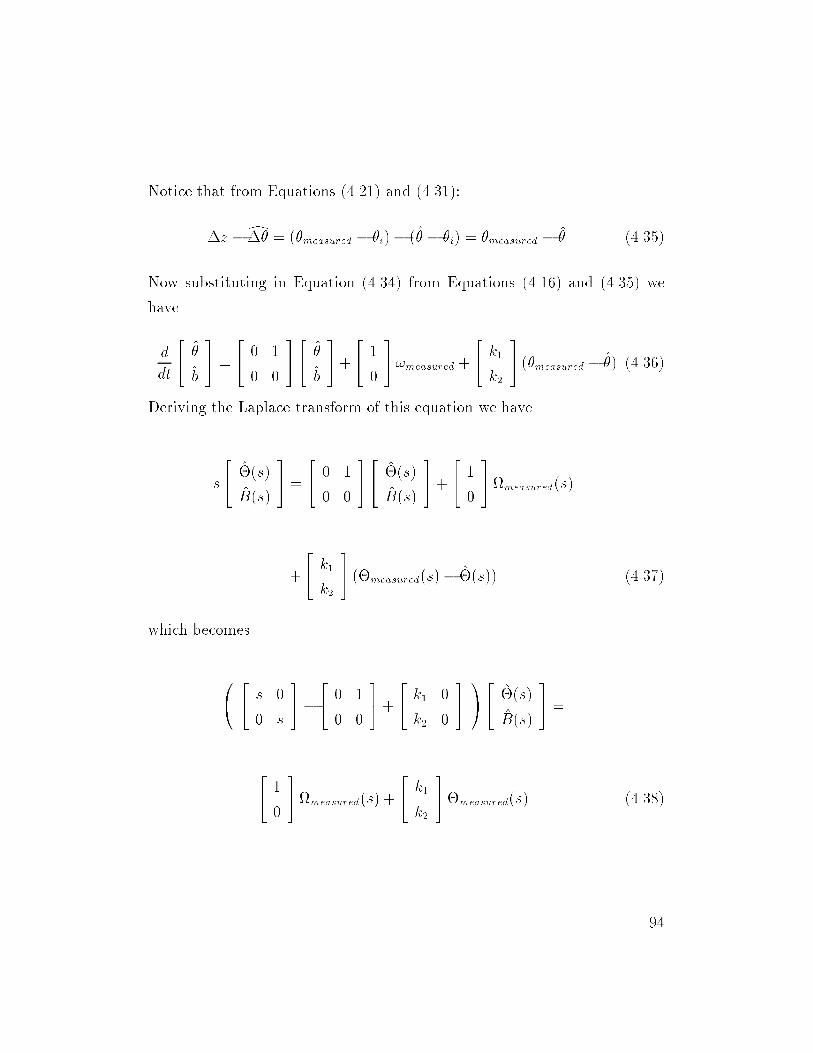
Notice that from Equations (4.21) and (4.31):
z d = (measured i) ( i) = measured (4.35)
Now substituting in Equation (4.34) from Equations (4.16) and (4.35) we
have
d
dt
24
b
35 =
24 0 1
0 0
3524
b
35+
24 1
0
35!measured +
24 k1
k2
35 (measured ) (4.36)
Deriving the Laplace transform of this equation we have
s
24 (s)
B(s)
35 =
24 0 1
0 0
3524 (s)
B(s)
35+
24 1
0
35measured(s)
+
24 k1
k2
35 (measured(s) (s)) (4.37)
which becomes
0@24 s 0
0 s
35
24 0 1
0 0
35+
24 k1 0
k2 0
351A24 (s)
B(s)
35 =
24 1
0
35measured(s) +
24 k1
k2
35measured(s) (4.38)
94
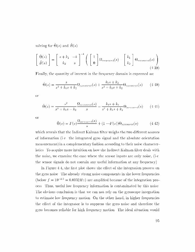
solving for (s) and B(s)
24 (s)
B(s)
35 =
24 s+ k1 1
k2 s
3510@24 1
0
35measured(s) +
24 k1
k2
35measured(s)
1A
(4.39)
Finally, the quantity of interest in the frequency domain is expressed as:
(s) =s
s2 + k1s+ k2measured(s) +
k1s + k2
s2 + k1s+ k2measured(s) (4.40)
or
(s) =s2
s2 + k1s+ k2
measured(s)
s+
k1s+ k2
s2 + k1s+ k2measured(s) (4.41)
or
(s) = F (s)measured(s)
s+ (1 F (s))measured(s) (4.42)
which reveals that the Indirect Kalman lter weighs the two dierent sources
of information (i.e. the integrated gyro signal and the absolute orientation
measurement) in a complementary fashion according to their noise character-
istics. To acquire more intuition on how the Indirect Kalman lter deals with
the noise, we examine the case where the sensor inputs are only noise, (i.e.
the sensor signals do not contain any useful information at any frequency).
In Figure 4.4, the rst plot shows the eect of the integration process on
the gyro noise. The already strong noise components in the lower frequencies
(below f = 102:5 = 0:0032Hz) are amplied because of the integration pro-
cess. Thus, useful low frequency information is contaminated by this noise.
The obvious conclusion is that we can not rely on the gyroscope integration
to estimate low frequency motion. On the other hand, in higher frequencies
the eect of the integrator is to suppress the gyro noise and therefore the
gyro becomes reliable for high frequency motion. The ideal situation would
95
be to fuse the integrated gyro information with a sensor (an absolute orien-
tation sensor such as a sun sensor, for example) that has a complementary
noise prole (i.e. the noise is small at lower frequencies and becomes larger
at higher frequencies) or at least has a constant noise prole, the same for
all frequencies. The second case has been assumed and the noise proles of
both the integrated gyro and the absolute orientation sensor are depicted in
the second plot of Figure 4.4.
At this point we should clarify how the Indirect Kalman lter optimally
combines the information from the two dierent sources by examining it as
a signal processing entity. The explanation comes from the third plot of
Figure 4.4. Function F (s) which lters the integrated gyro signal works as a
high pass lter. It suppresses the low frequency noise content and allows the
higher frequencies to pass undistorted. To the contrary, the complementary
function 1 F (s) lters the absolute orientation sensor and acts as a low
pass lter. It allows the critical low frequency information from the absolute
orientation sensor to pass undistorted while reduces its strength in the higher
frequencies. This is desired since the estimator performs better if it relies on
the gyro in that range.
4.1.3.4 Observability
Measuring Orientation Continuously:
The observability matrix of the system is:
HT
... F T HT
=
24 1 0
0 1
35 (4.43)
Clearly it has rank 2. Thus the system is observable and the uncertainty for
both states (orientation and bias) is bounded. This can be seen in Figure
96
4.5. Both covariances reach a steady state.4 It is worth noticing that though
the bias is not directly measured it can be estimated. This is shown in Figure
4.6.
Measuring Orientation Intermittently:
In this case the observability matrix
HT
... F T HT
=
24 0 0
0 0
35 (4.44)
loses its rank for those time intervals for which we do not have an absolute
measurement of the orientation. This can be seen graphically in Figure 4.7.
The covariances (which capture the uncertainty) of both the orientation and
the bias grow without bounds until a new measurement from the absolute
orientation sensor is received. This causes a decrease in the uncertainty which
then begins to grow as before. Following this strategy (i.e. taking an ab-
solute orientation measurement only at certain instants) produces the \saw
tooth" pattern in the covariance plot.5
The formal explanation is provided by the discrete Kalman lter formula-
tion for the covariance:
Pk;k1 = (k; k 1)Pk1;k1(k; k 1)T +Qk1 (4.45)
Pk;k = Pk;k1 Pk;k1HTk [HkPk;k1H
Tk +Rk]
1HkPk;k1 (4.46)
4The covariance matrix P calculated in the Kalman lter is dened as:
P = Ef
b
b
g =
2
;b
b; 2b
The covariance of the orientation estimate and of the bias estimate b are given by the
rst and the second diagonal element of this matrix, respectively.5This observation was rst reported in [71].
97
where Pk1;k1 is the covariance matrix from the previous step (time tk1,
measurements up to k 1), Pk;k1 is the propagated covariance (time tk,
measurements up to k 1), Pk;k is the updated covariance after the new ab-
solute orientation measurement (time tk, measurements up to k), (k; k1)
is the state transition matrix from time step tk1 to time step tk, Hk is the
measurement matrix at time tk, Qk is the system noise covariance matrix at
time tk and Rk is the measurement noise covariance matrix at time tk.
Equation (4.45) represents the increase in the system uncertainty at ev-
ery time step due to the previous propagated system uncertainty and the
newly added system noise. This equation is valid at every time step and
causes the covariance to grow without bounds. Equation (4.46) is applied
only when a new measurement arrives. It reduces the value of the propagated
covariance matrix Pk;k1 since it subtracts from it a positive denite matrix
( Pk;k1HTk [HkPk;k1H
Tk +Rk]
1HkPk;k1). The smaller the matrix Rk (i.e.
the better the quality of the absolute orientation measurement), the larger
the decrease.
Here we focus on how the Indirect Kalman lter tracks the bias in the
case that the system is observable only at certain time instants. In Figure
4.8 we see that, in the absence of any other information, the lter assumes
that the bias is constant. When a new absolute orientation measurement is
introduced, the lter updates the bias estimate according to the cumulative
eect of the bias on the error in orientation during the preceding time in-
terval. After that the bias is assumed again to be constant, until the next
measurement.
It is obvious that in the long run, uncertainty in orientation is bounded.
It will not exceed a certain limit depending on the frequency of the absolute
orientation updates and on the accuracy of this sensor along with the noise
98
prole of the gyro and its bias. Thus, the frequency of the absolute mea-
surements is a design parameter that the system engineer can select based
on mission specic constraints.
4.1.3.5 Backward lter
At this point we revisit the initial problem at hand. We built an Indirect
Kalman lter that estimates the vehicle orientation mainly because we need
the attitude information to calculate the position update of the rover. The
orientation information is required at every time step (Equations (4.1) and
(4.2)) and its accuracy is crucial for precise position estimation. As we can
see from the orientation covariance plot in Figure 4.7 the covariance of the
estimate reaches its maximum right before a new absolute orientation mea-
surement. During the preceding time instants, the orientation information
becomes increasingly untrustworthy and the validity of the position updates
that depend on it, decays.
In the proposed novel approach we take advantage of the fact that the
uncertainty decreases considerably right after the absolute orientation mea-
surement at some time tk. We apply a backward propagation of the Indirect
Kalman lter every time we receive a good estimate of the orientation (i.e.
when a new absolute orientation measurement is introduced). In the back-
ward propagation the initial condition for the state is the updated (corrected)
state estimate at time tk. Then a backward integration using the previously
acquired (stored) gyro values is performed to calculate the orientation at
each previous time instant up to the last absolute orientation measurement
at time tkM . The eect is to obtain more accurate estimates for the interval
preceding time tk. These estimates will have the same behavior when they
move away (in the backward time direction) from tk as the forward lter
99
estimates have when they move away from time tkM (previous absolute ori-
entation measurement). As the backward lter estimates get closer to tkM
their covariance increases and the quality of the estimate decreases. This is
clearly shown in Figure 4.9. To better understand the functionality of the
backward lter we examine the equations that govern it as presented in [29].
If the system equation is
_x = Fx+ n (4.47)
then by substituting
= T t (4.48)
where is the backward time variable and
T = tk tkM (4.49)
is the time interval of smoothing, the backward system equation can be
derived from:dx
d=
dx
dt
dt
d= _x (4.50)
and is:dxb
d= Fxb n (4.51)
The continuous time covariance propagation equation for the forward lter
is:
_P = FP + PF T +Q (4.52)
and correspondingly the covariance backwards propagation equation would
be:
_Pb = FPb PbFT +Q (4.53)
100
In the discrete time domain the previous equation becomes:
Pb(k1;k) = (k 1; k)Pb(k;k)(k 1; k)T +Qk (4.54)
which is of the same form as Equation (4.45) and thus the covariance of
the backward lter also increases during propagation in the same manner as
the forward lter's covariance. The main dierence is that Pb starts from a
small value at time tk and grows as it moves towards tkM . These results are
depicted in Figure 4.9 for the orientation covariance. In Figure 4.10 we can
see the performance of the backward lter for the variable of interest, the
orientation. The orientation estimate for the backward lter is close to its
true value for t = 400sec and deviates from it as it reaches close to t = 200sec.
The next step is to optimally combine the forward and the backward lter
estimates in the smoother.
4.1.3.6 Smoother
The smoother combines the estimates of the forward and the backward
Kalman lter to provide estimates of the state at every time as if all the
measurements during the entire smoothing interval were available. The to-
tal (smoothed) result outperforms both lters. This is evident in Figure 4.9
where the total covariance (or smoothed covariance) is at all times smaller
than the smallest of the two lters. This can be explained by examining the
equation for the smoothed covariance [56]:
P1total = P1f + P1b (4.55)
101
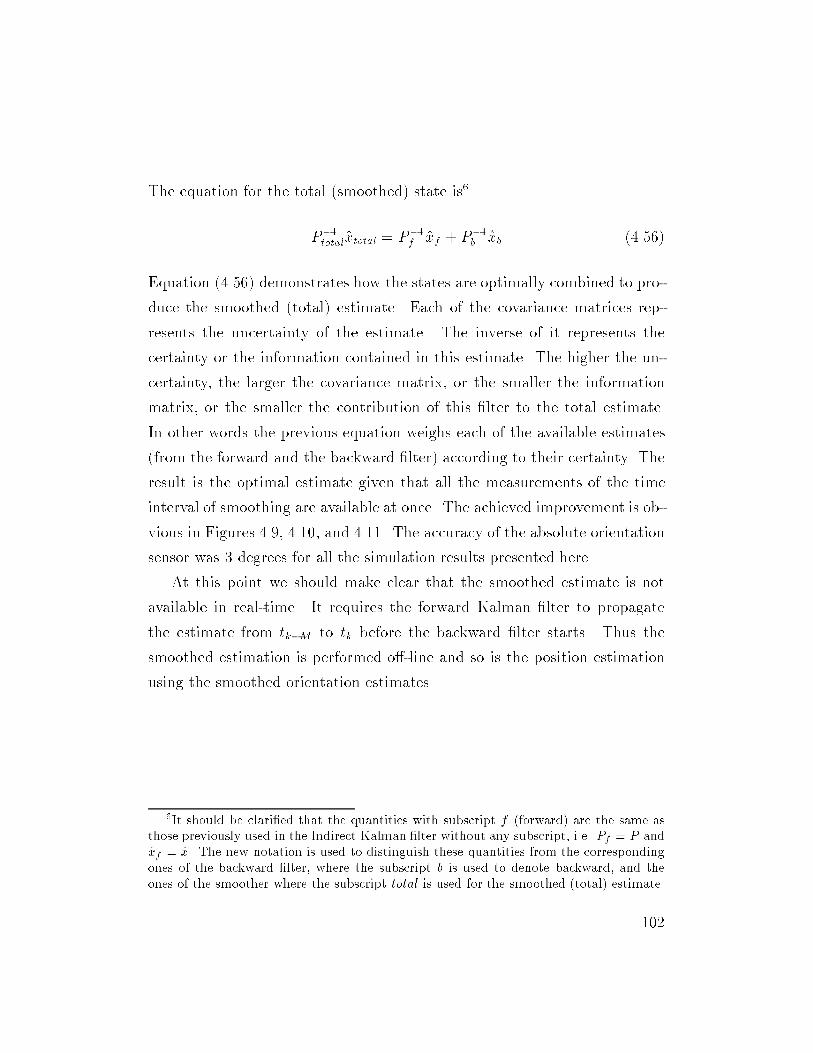
The equation for the total (smoothed) state is6
P1totalxtotal = P1f xf + P1b xb (4.56)
Equation (4.56) demonstrates how the states are optimally combined to pro-
duce the smoothed (total) estimate. Each of the covariance matrices rep-
resents the uncertainty of the estimate. The inverse of it represents the
certainty or the information contained in this estimate. The higher the un-
certainty, the larger the covariance matrix, or the smaller the information
matrix, or the smaller the contribution of this lter to the total estimate.
In other words the previous equation weighs each of the available estimates
(from the forward and the backward lter) according to their certainty. The
result is the optimal estimate given that all the measurements of the time
interval of smoothing are available at once. The achieved improvement is ob-
vious in Figures 4.9, 4.10, and 4.11. The accuracy of the absolute orientation
sensor was 3 degrees for all the simulation results presented here.
At this point we should make clear that the smoothed estimate is not
available in real-time. It requires the forward Kalman lter to propagate
the estimate from tkM to tk before the backward lter starts. Thus the
smoothed estimation is performed o-line and so is the position estimation
using the smoothed orientation estimates.
6It should be claried that the quantities with subscript f (forward) are the same as
those previously used in the Indirect Kalman lter without any subscript, i.e. Pf = P and
xf = x. The new notation is used to distinguish these quantities from the corresponding
ones of the backward lter, where the subscript b is used to denote backward, and the
ones of the smoother where the subscript total is used for the smoothed (total) estimate.
102
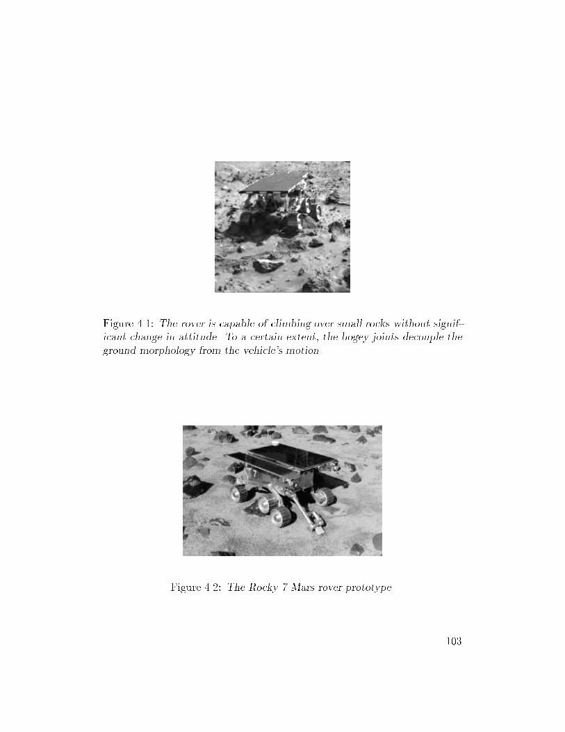
Figure 4.1: The rover is capable of climbing over small rocks without signif-
icant change in attitude. To a certain extent, the bogey joints decouple the
ground morphology from the vehicle's motion.
Figure 4.2: The Rocky 7 Mars rover prototype.
103
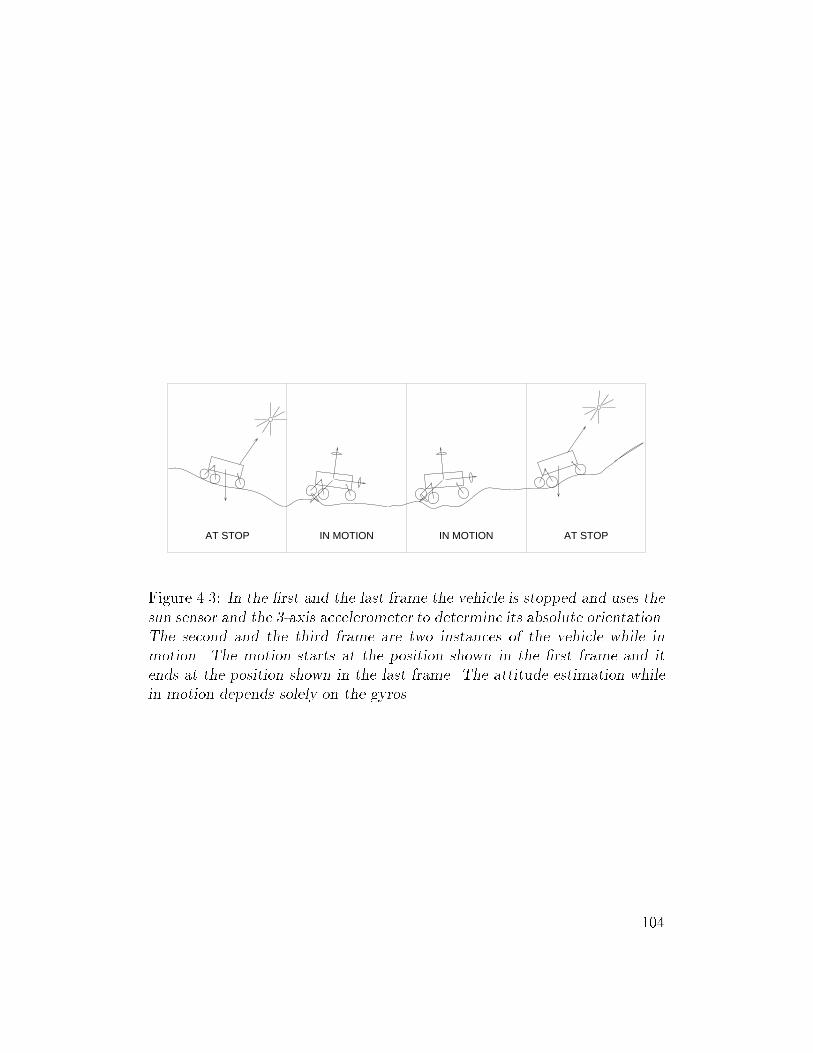
AT STOPIN MOTIONAT STOP IN MOTION
Figure 4.3: In the rst and the last frame the vehicle is stopped and uses the
sun sensor and the 3-axis accelerometer to determine its absolute orientation.
The second and the third frame are two instances of the vehicle while in
motion. The motion starts at the position shown in the rst frame and it
ends at the position shown in the last frame. The attitude estimation while
in motion depends solely on the gyros.
104
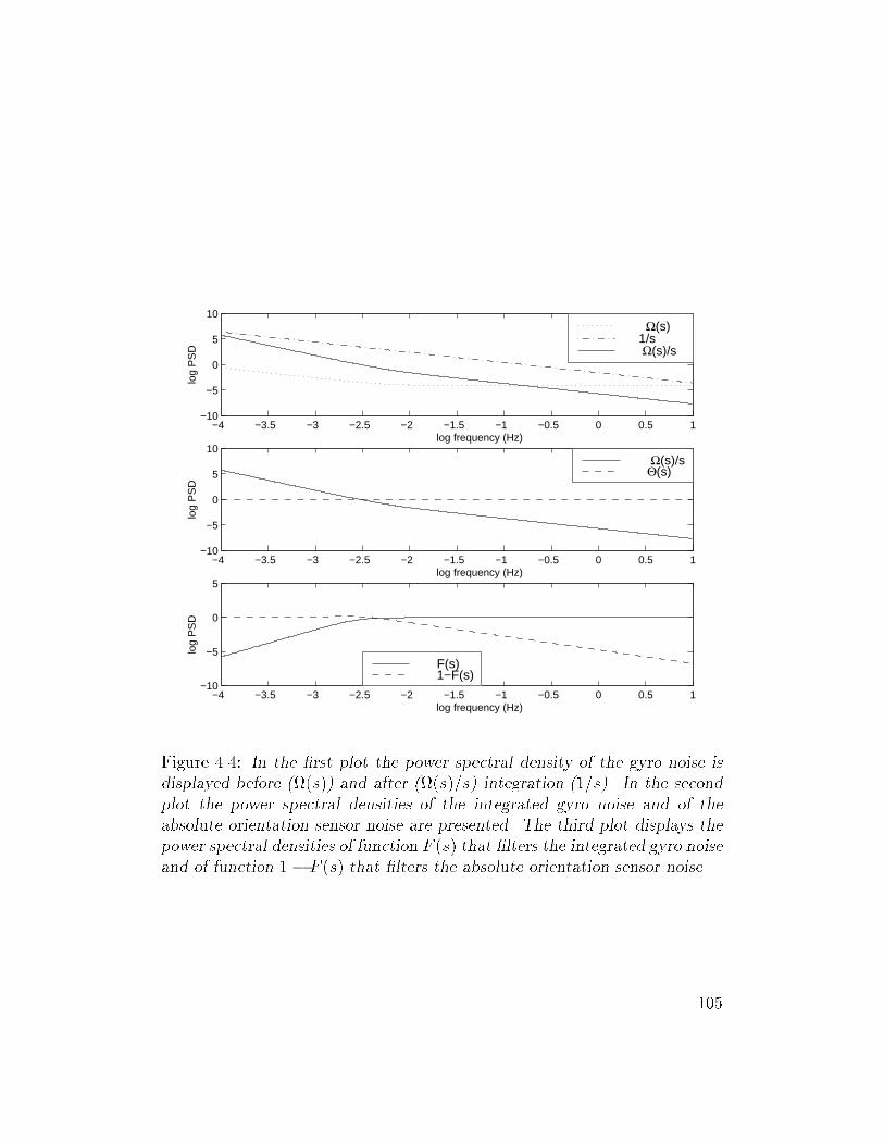
−4 −3.5 −3 −2.5 −2 −1.5 −1 −0.5 0 0.5 1−10
−5
0
5
10
log frequency (Hz)
log
PS
D
Ω(s)1/s Ω(s)/s
−4 −3.5 −3 −2.5 −2 −1.5 −1 −0.5 0 0.5 1−10
−5
0
5
10
log
PS
D
log frequency (Hz)
Ω(s)/s Θ(s)
−4 −3.5 −3 −2.5 −2 −1.5 −1 −0.5 0 0.5 1−10
−5
0
5
log
PS
D
log frequency (Hz)
F(s) 1−F(s)
Figure 4.4: In the rst plot the power spectral density of the gyro noise is
displayed before ((s)) and after ((s)=s) integration (1=s). In the second
plot the power spectral densities of the integrated gyro noise and of the
absolute orientation sensor noise are presented. The third plot displays the
power spectral densities of function F (s) that lters the integrated gyro noiseand of function 1 F (s) that lters the absolute orientation sensor noise.
105
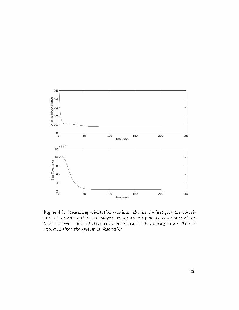
0 50 100 150 200 2500
0.1
0.2
0.3
0.4
0.5
Orie
ntat
ion
Cov
aria
nce
time (sec)
0 50 100 150 200 2502
4
6
8
10
12x 10
−4
Bia
s C
ovar
ianc
e
time (sec)
Figure 4.5: Measuring orientation continuously: In the rst plot the covari-
ance of the orientation is displayed. In the second plot the covariance of the
bias is shown. Both of these covariances reach a low steady state. This is
expected since the system is observable.
106
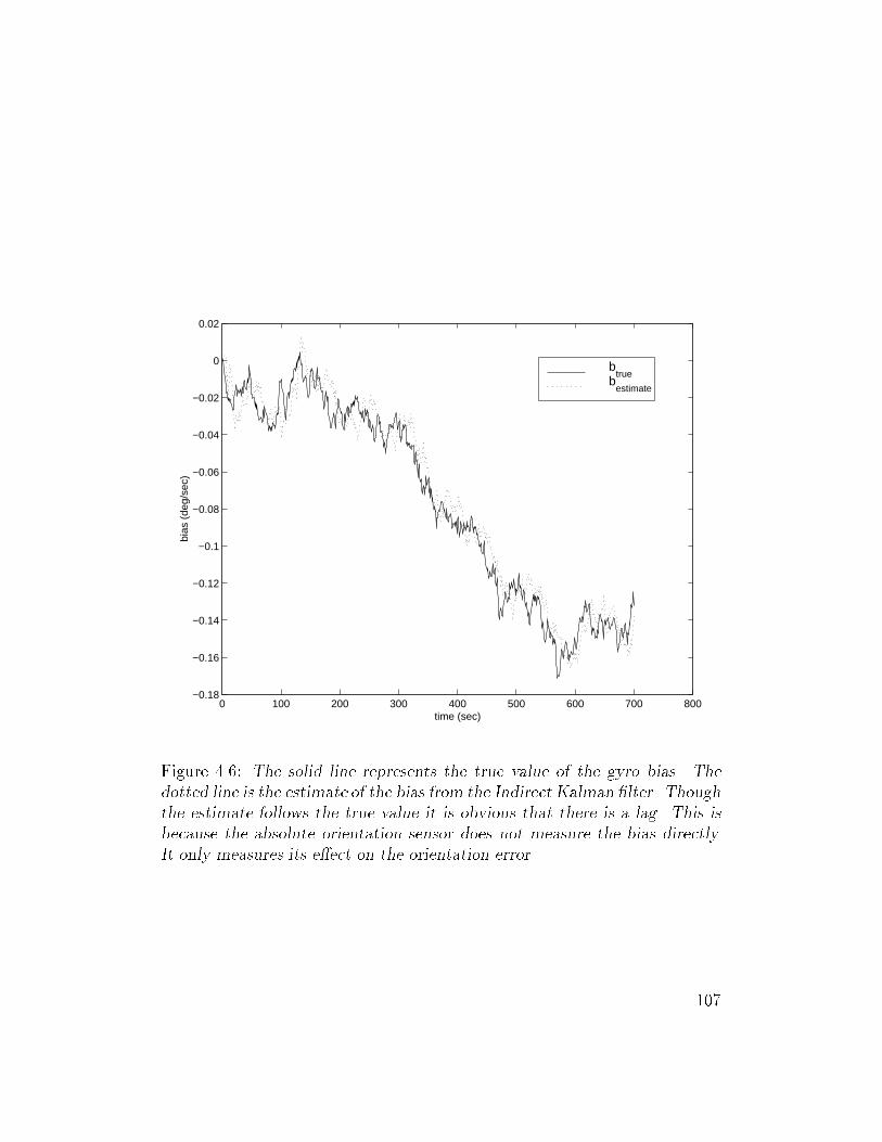
0 100 200 300 400 500 600 700 800−0.18
−0.16
−0.14
−0.12
−0.1
−0.08
−0.06
−0.04
−0.02
0
0.02
bias
(de
g/se
c)
time (sec)
btrue
bestimate
Figure 4.6: The solid line represents the true value of the gyro bias. The
dotted line is the estimate of the bias from the Indirect Kalman lter. Though
the estimate follows the true value it is obvious that there is a lag. This is
because the absolute orientation sensor does not measure the bias directly.
It only measures its eect on the orientation error.
107
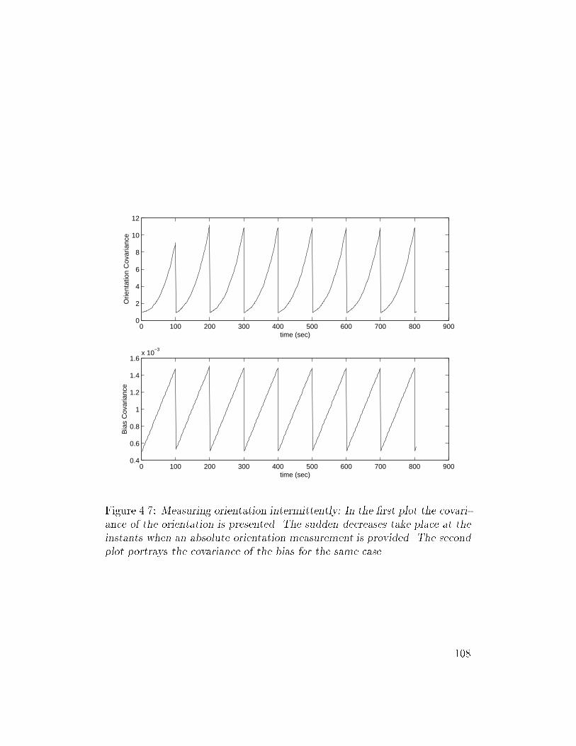
0 100 200 300 400 500 600 700 800 9000
2
4
6
8
10
12
Orie
ntat
ion
Cov
aria
nce
time (sec)
0 100 200 300 400 500 600 700 800 9000.4
0.6
0.8
1
1.2
1.4
1.6x 10
−3
Bia
s C
ovar
ianc
e
time (sec)
Figure 4.7: Measuring orientation intermittently: In the rst plot the covari-
ance of the orientation is presented. The sudden decreases take place at the
instants when an absolute orientation measurement is provided. The second
plot portrays the covariance of the bias for the same case.
108
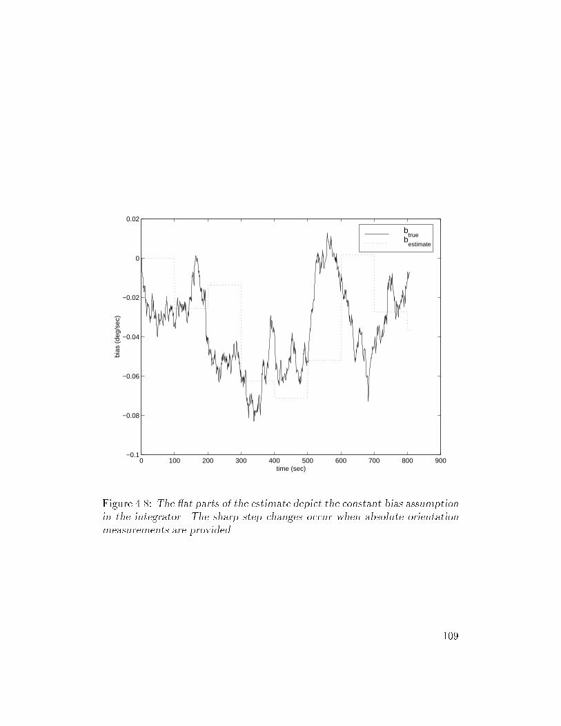
0 100 200 300 400 500 600 700 800 900−0.1
−0.08
−0.06
−0.04
−0.02
0
0.02
bias
(de
g/se
c)
time (sec)
btrue
bestimate
Figure 4.8: The at parts of the estimate depict the constant bias assumption
in the integrator. The sharp step changes occur when absolute orientation
measurements are provided.
109
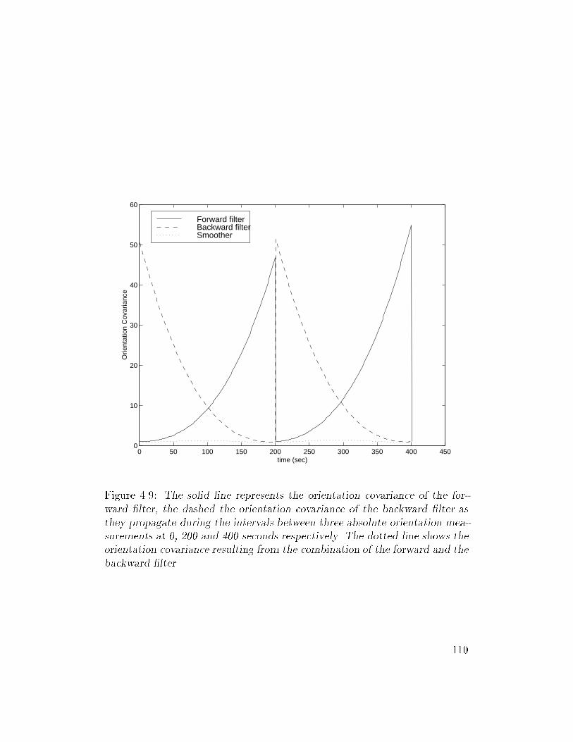
0 50 100 150 200 250 300 350 400 4500
10
20
30
40
50
60
time (sec)
Orie
ntat
ion
Cov
aria
nce
Forward filterBackward filterSmoother
Figure 4.9: The solid line represents the orientation covariance of the for-
ward lter, the dashed the orientation covariance of the backward lter as
they propagate during the intervals between three absolute orientation mea-
surements at 0, 200 and 400 seconds respectively. The dotted line shows the
orientation covariance resulting from the combination of the forward and the
backward lter.
110
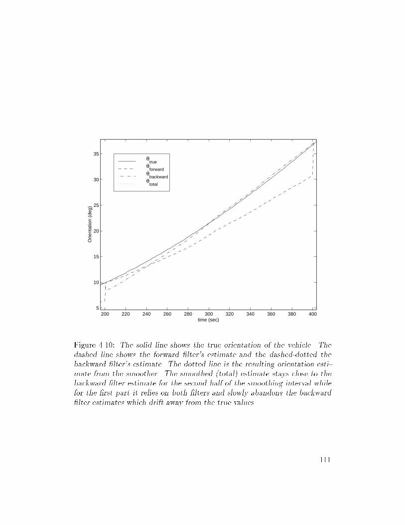
200 220 240 260 280 300 320 340 360 380 4005
10
15
20
25
30
35
Orie
ntat
ion
(deg
)
time (sec)
θtrue
θforward
θbackward
θtotal
Figure 4.10: The solid line shows the true orientation of the vehicle. The
dashed line shows the forward lter's estimate and the dashed-dotted the
backward lter's estimate. The dotted line is the resulting orientation esti-
mate from the smoother. The smoothed (total) estimate stays close to the
backward lter estimate for the second half of the smoothing interval while
for the rst part it relies on both lters and slowly abandons the backward
lter estimates which drift away from the true values.
111
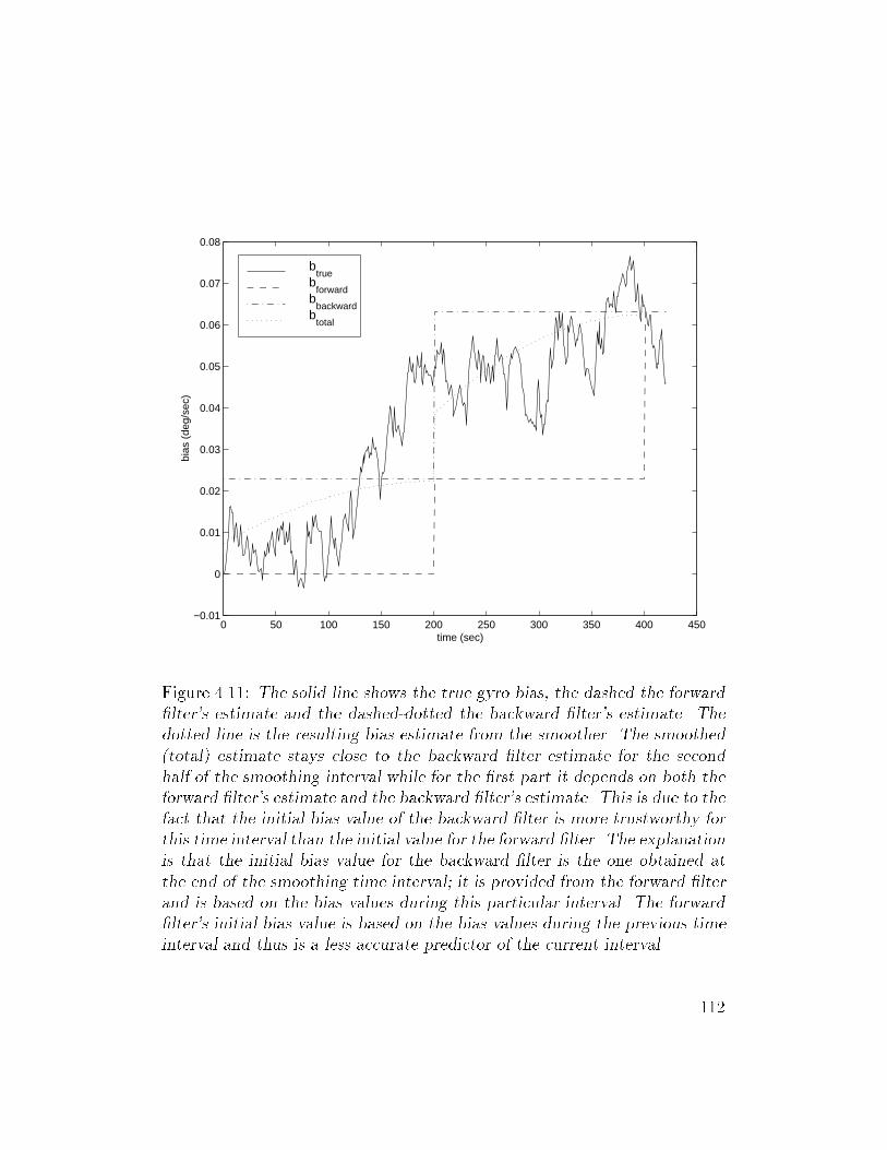
0 50 100 150 200 250 300 350 400 450−0.01
0
0.01
0.02
0.03
0.04
0.05
0.06
0.07
0.08
bias
(de
g/se
c)
time (sec)
btrue
bforward
bbackward
btotal
Figure 4.11: The solid line shows the true gyro bias, the dashed the forward
lter's estimate and the dashed-dotted the backward lter's estimate. The
dotted line is the resulting bias estimate from the smoother. The smoothed
(total) estimate stays close to the backward lter estimate for the second
half of the smoothing interval while for the rst part it depends on both the
forward lter's estimate and the backward lter's estimate. This is due to the
fact that the initial bias value of the backward lter is more trustworthy for
this time interval than the initial value for the forward lter. The explanation
is that the initial bias value for the backward lter is the one obtained at
the end of the smoothing time interval; it is provided from the forward lter
and is based on the bias values during this particular interval. The forward
lter's initial bias value is based on the bias values during the previous time
interval and thus is a less accurate predictor of the current interval.
112
Chapter 5
Smoother Based Attitude Estimation 3-D
5.1 Introduction
In the previous chapter we demonstrated the smoother based attitude esti-
mation methodology for the case of planar motion. The linear form of the
system and measurement equations allowed us to study observability ana-
lytically and examine the role of the Kalman lter as a signal processing
unit that weighs the sensory information according to its noise power spec-
tral density prole. We also demonstrated the improvement in the overall
quality of the attitude estimate when the smoother was involved. The lack
of observability for the largest part of the trajectory forces the covariance
of the estimate to steadily increase after each absolute measurement. The
increase of the uncertainty is due to the gyro noise and bias-drift. During
the instants of observability, the accumulated eect of the gyro noise is can-
celed and precise attitude information is provided to the lter. The estimate
becomes trustworthy only for a limited time. As the vehicle moves the qual-
ity of the attitude estimate decreases . Any algorithm that computes the
position of the robot using these attitude estimates will drift. This anomaly
manifests itself as a saw-tooth pattern in the time prole of the covariance
113
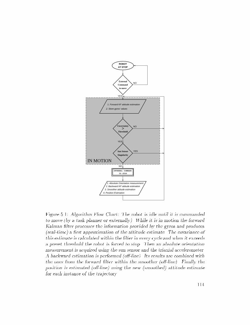
ROBOTAT STOP
External
Command
to move
INTERNAL COMMAND
TO STOP
NO
NO
YES
Sun Sensor
Uncertainty>
2. Store gyros’ values
NO
YES
YES
IN MOTION
1. Absolute Orientation measurement2. Backward KF attitude estimation
3. Smoother attitude estimation
4. Position Estimation
1. Forward KF attitude estimation
Threshold
Singularity
Figure 5.1: Algorithm Flow Chart: The robot is idle until it is commanded
to move (by a task planner or externally). While it is in motion the forward
Kalman lter processes the information provided by the gyros and produces
(real-time) a rst approximation of the attitude estimate. The covariance of
this estimate is calculated within the lter in every cycle and when it exceeds
a preset threshold the robot is forced to stop. Then an absolute orientation
measurement is acquired using the sun sensor and the triaxial accelerometer.
A backward estimation is performed (o-line). Its results are combined with
the ones from the forward lter within the smoother (o-line). Finally the
position is estimated (o-line) using the new (smoothed) attitude estimate
for each instance of the trajectory.
114
of the estimate. A smoother can be used when the system is observable only
during certain time instants. The smoother computes the best estimates of
the attitude during a certain time interval provided all the measurements
collected during this time. These measurements include the initial absolute
orientation, all the intermediate (inertial) readings from the gyros, and the
nal absolute orientation. This last measurement marks the end of this time
interval and the beginning of the next one. The improvement is larger for
those parts of the trajectory during which the estimate is of the lowest qual-
ity, i.e. for the instants right before an absolute measurement. In this way,
we are able to sustain uniformly lower levels of uncertainty throughout the
duration of the motion.
In this section we apply these ideas to a rover on the surface of Mars.
As in almost every outdoor environment, 3D localization is required for the
robot to position itself accurately with respect to a known initial position
(i.e. landing site). The assumption of at and horizontal ground, frequently
used for indoor applications, fails dramatically. When the rover moves on
slopes (inclined planes) precise orientation is needed to correct the position
estimates. Neglecting the roll and pitch information, not only degrades the
localization accuracy but can also endanger the completion of the mission.
All terrain navigation requires estimates of the roll and pitch angles to ensure
vehicle safety. In addition, proper interpretation of external sensor data (e.g.
vision) needs attitude information in order to construct an accurate model
of the environment. The potential sensors on-board the rover are three gy-
roscopes, a sun sensor and an accelerometer. As mentioned before, when
the vehicle moves on the cratered, rocky slopes of the planet the gyros are
the only source of attitude information. When it stops, the accelerometer
measures solely the gravitational acceleration and thus determines the unit
vector of the local vertical (roll and pitch information). Simultaneously, the
115
sun sensor locates the position of the sun in the sky and thus species the
heading of the vehicle (yaw information). This is the absolute orientation of
the vehicle and it is available only at stop.
The proposed method is summarized in the following algorithm (Figure
5.1): The vehicle is commanded to move for some time. A (forward) Indirect
Kalman lter processes the incoming gyro values (angular velocities) and
provides an initial real-time attitude estimate. The gyro values are stored
for later processing. The covariance of the estimate is monitored and when
it becomes unreliable the vehicle stops. Then, another absolute orientation
measurement is collected and the smoother is activated. The backward lter
uses the last (absolute) measurement and propagates the orientation esti-
mate backwards using the stored values of angular velocity measurements.
Finally, the resulting estimates are combined with the previous ones (from
the forward lter) and the smoothed attitude estimate is passed to the posi-
tion estimating module.
This new method is not limited to robots used for extra-terrestrial explo-
ration. It can also be applied to other autonomous vehicles equipped with
an equivalent set of sensors. The mixing of high frequency inertial sensors
with usually lower frequency absolute (position or orientation) sensors is be-
coming very common in mobile robotics. Robots on earth equipped with
GPS or landmark tracking devices often carry additional sensors that can be
used for localization when the GPS signal is unavailable or the landmarks are
occluded. These additional encoders or inertial sensors increase the overall
redundancy of the system. The presented framework can be used to opti-
mally combine them with the absolute sensors.
116
5.1.1 Quaternions in Attitude Representation
The three-parameter Euler angle representation has been used in most ap-
plications of the Kalman lter in robot localization [28], [7]. However the
kinematic equations for Euler angles involve non-linear and computationally
expensive trigonometric functions. The computational cost using quaternions
is less than using Euler angles.1 It is also more compact because only four pa-
rameters, rather than nine, are needed. Furthermore in the Euler angle rep-
resentation the angles become undened for some rotations (the gimbal lock
situation) which causes problems in Kalman ltering applications. Amongst
all the representations for nite rotations, only those of four parameters be-
have well for arbitrary rotations. The reason is that a non-singular mapping
between parameters and their corresponding rotational transformation ma-
trix requires a set of at least four parameters. This issue was addressed by
Stuelpnagel [86].
Quaternions provide an elegant and convenient parameterization of the
attitude. A unit quaternion is a global non-singular four parameter repre-
sentation also known as Euler symmetric parameters. Physical quantities
pertaining to the motion of rotation such as angular displacement, velocity,
acceleration and momentum are derived in terms of Euler parameters in a
simple manner. Manipulating equations is much easier when using quater-
nion algebra [13]. The generalized commutative properties of quaternion
multiplication are very useful when combining kinematic equations derived
from successive rotations in space. Quaternions were invented by Hamilton
in 1843 [36]. Their use in simulation of attitude dynamics was promoted by
1For quaternions there is a relatively simple form for combining the parameters for
two individual rotations to give the parameters of the product of the two rotations; 16
multiplications are required. In the case of Euler angles, combination of two individual
rotations is done through attitude matrix multiplication; 27 multiplications are required.
117
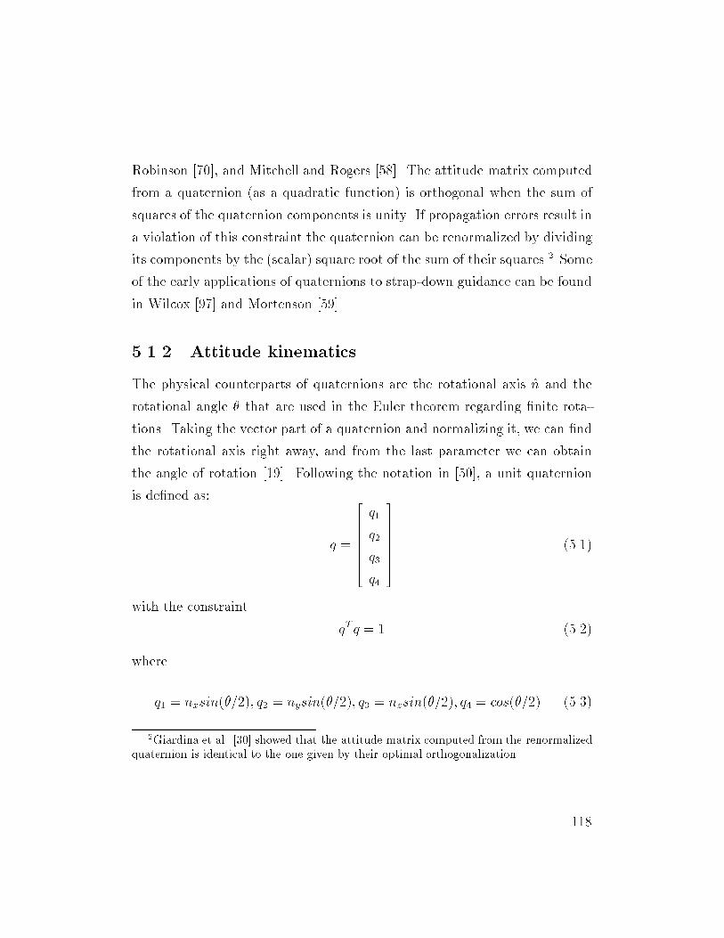
Robinson [70], and Mitchell and Rogers [58]. The attitude matrix computed
from a quaternion (as a quadratic function) is orthogonal when the sum of
squares of the quaternion components is unity. If propagation errors result in
a violation of this constraint the quaternion can be renormalized by dividing
its components by the (scalar) square root of the sum of their squares.2 Some
of the early applications of quaternions to strap-down guidance can be found
in Wilcox [97] and Mortenson [59].
5.1.2 Attitude kinematics
The physical counterparts of quaternions are the rotational axis n and the
rotational angle that are used in the Euler theorem regarding nite rota-
tions. Taking the vector part of a quaternion and normalizing it, we can nd
the rotational axis right away, and from the last parameter we can obtain
the angle of rotation [19]. Following the notation in [50], a unit quaternion
is dened as:
q =
26666664
q1
q2
q3
q4
37777775 (5.1)
with the constraint
qTq = 1 (5.2)
where
q1 = nxsin(=2); q2 = nysin(=2); q3 = nzsin(=2); q4 = cos(=2) (5.3)
2Giardina et al. [30] showed that the attitude matrix computed from the renormalized
quaternion is identical to the one given by their optimal orthogonalization.
118
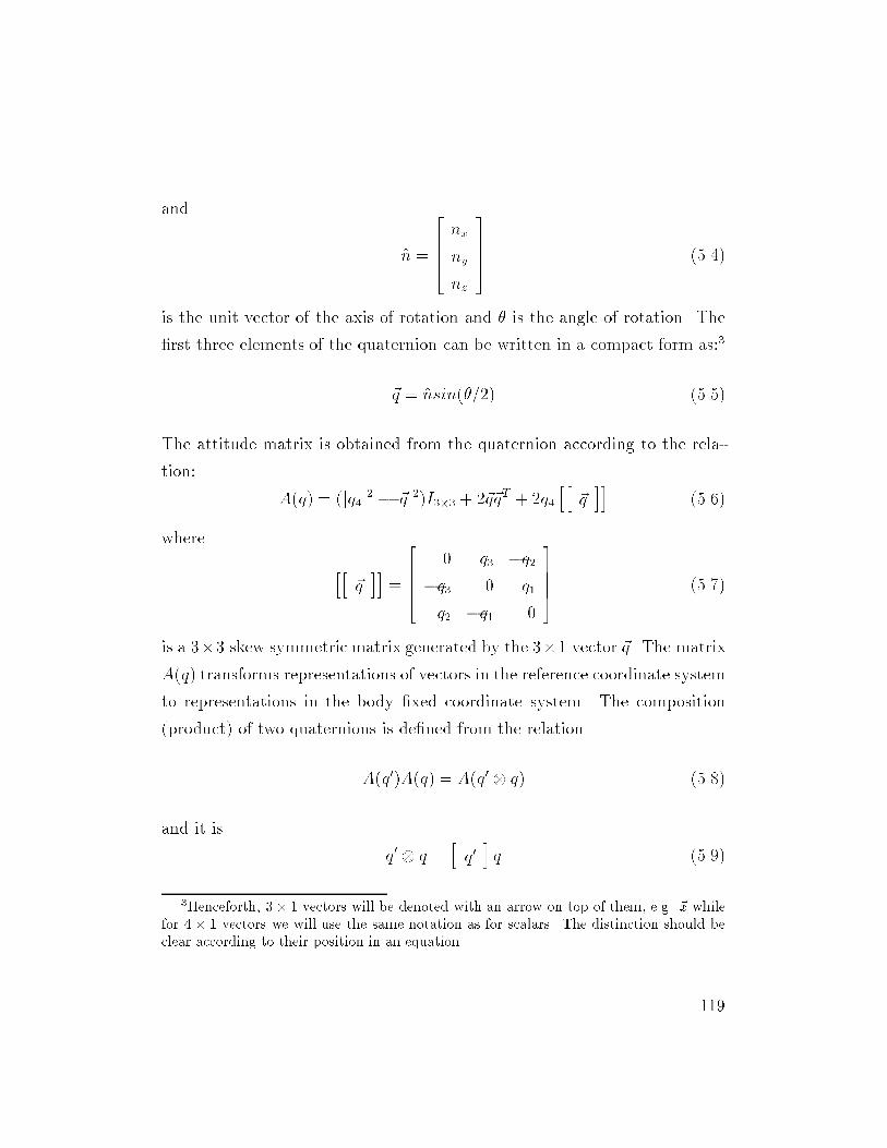
and
n =
26664nx
ny
nz
37775 (5.4)
is the unit vector of the axis of rotation and is the angle of rotation. The
rst three elements of the quaternion can be written in a compact form as:3
~q = nsin(=2) (5.5)
The attitude matrix is obtained from the quaternion according to the rela-
tion:
A(q) = (jq4j2 j~qj2)I33 + 2~q~qT + 2q4hh
~qii
(5.6)
where
hh~qii=
26664
0 q3 q2q3 0 q1
q2 q1 0
37775 (5.7)
is a 33 skew symmetric matrix generated by the 31 vector ~q. The matrix
A(q) transforms representations of vectors in the reference coordinate system
to representations in the body xed coordinate system. The composition
(product) of two quaternions is dened from the relation
A(q0)A(q) = A(q0 q) (5.8)
and it is
q0 q =hq0iq (5.9)
3Henceforth, 3 1 vectors will be denoted with an arrow on top of them, e.g. ~x while
for 4 1 vectors we will use the same notation as for scalars. The distinction should be
clear according to their position in an equation.
119
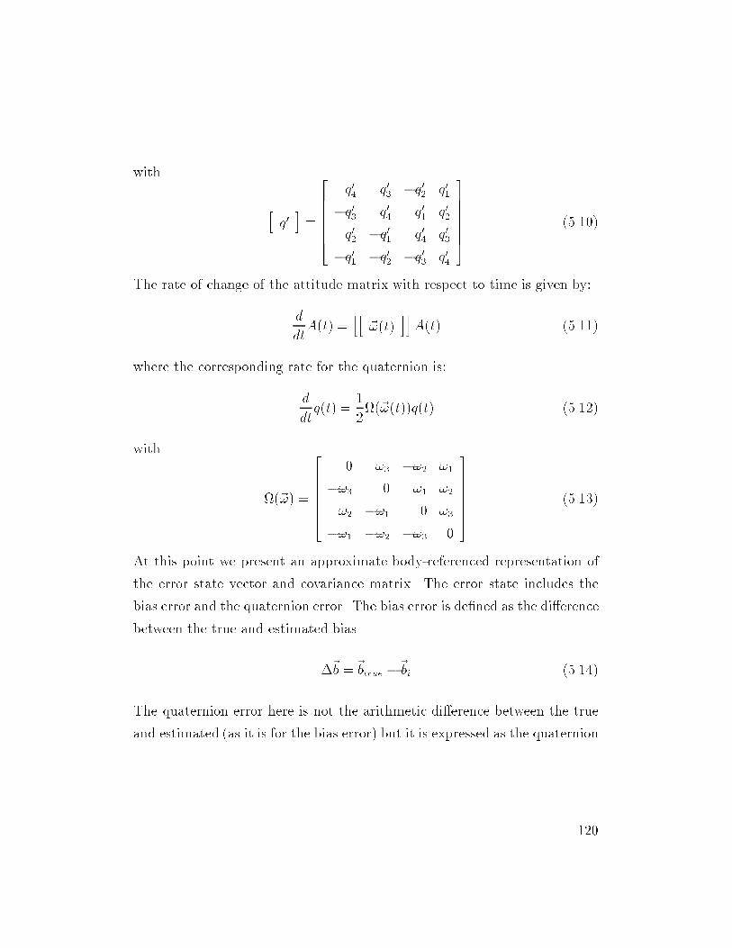
with
hq0i=
26666664
q04 q03 q02 q01
q03 q04 q01 q02
q02 q01 q04 q03
q01 q02 q03 q04
37777775 (5.10)
The rate of change of the attitude matrix with respect to time is given by:
d
dtA(t) =
hh~!(t)
iiA(t) (5.11)
where the corresponding rate for the quaternion is:
d
dtq(t) =
1
2(~!(t))q(t) (5.12)
with
(~!) =
26666664
0 !3 !2 !1
!3 0 !1 !2
!2 !1 0 !3
!1 !2 !3 0
37777775 (5.13)
At this point we present an approximate body-referenced representation of
the error state vector and covariance matrix. The error state includes the
bias error and the quaternion error. The bias error is dened as the dierence
between the true and estimated bias.
~b = ~btrue ~bi (5.14)
The quaternion error here is not the arithmetic dierence between the true
and estimated (as it is for the bias error) but it is expressed as the quaternion
120
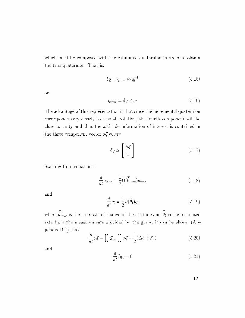
which must be composed with the estimated quaternion in order to obtain
the true quaternion. That is:
q = qtrue q1i (5.15)
or
qtrue = q qi (5.16)
The advantage of this representation is that since the incremental quaternion
corresponds very closely to a small rotation, the fourth component will be
close to unity and thus the attitude information of interest is contained in
the three component vector ~q where
q '
24 ~q
1
35 (5.17)
Starting from equations:
d
dtqtrue =
1
2(~_true)qtrue (5.18)
andd
dtqi =
1
2(~_i)qi (5.19)
where~_true is the true rate of change of the attitude and
~_i is the estimated
rate from the measurements provided by the gyros, it can be shown (Ap-
pendix B.1) thatd
dt~q =
hh~!m
ii~q
1
2(~b+ ~nr) (5.20)
andd
dtq4 = 0 (5.21)
121
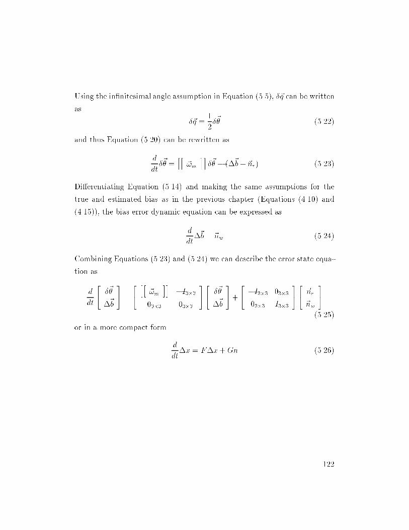
Using the innitesimal angle assumption in Equation (5.5), ~q can be written
as
~q =1
2~ (5.22)
and thus Equation (5.20) can be rewritten as
d
dt~ =
hh~!m
ii~ (~b+ ~nr) (5.23)
Dierentiating Equation (5.14) and making the same assumptions for the
true and estimated bias as in the previous chapter (Equations (4.10) and
(4.15)), the bias error dynamic equation can be expressed as
d
dt~b = ~nw (5.24)
Combining Equations (5.23) and (5.24) we can describe the error state equa-
tion as
d
dt
24 ~
~b
35 =
24hh
~!mii
I33033 033
3524 ~
~b
35+
24 I33 033
033 I33
3524 ~nr
~nw
35(5.25)
or in a more compact form
d
dtx = Fx+Gn (5.26)
122
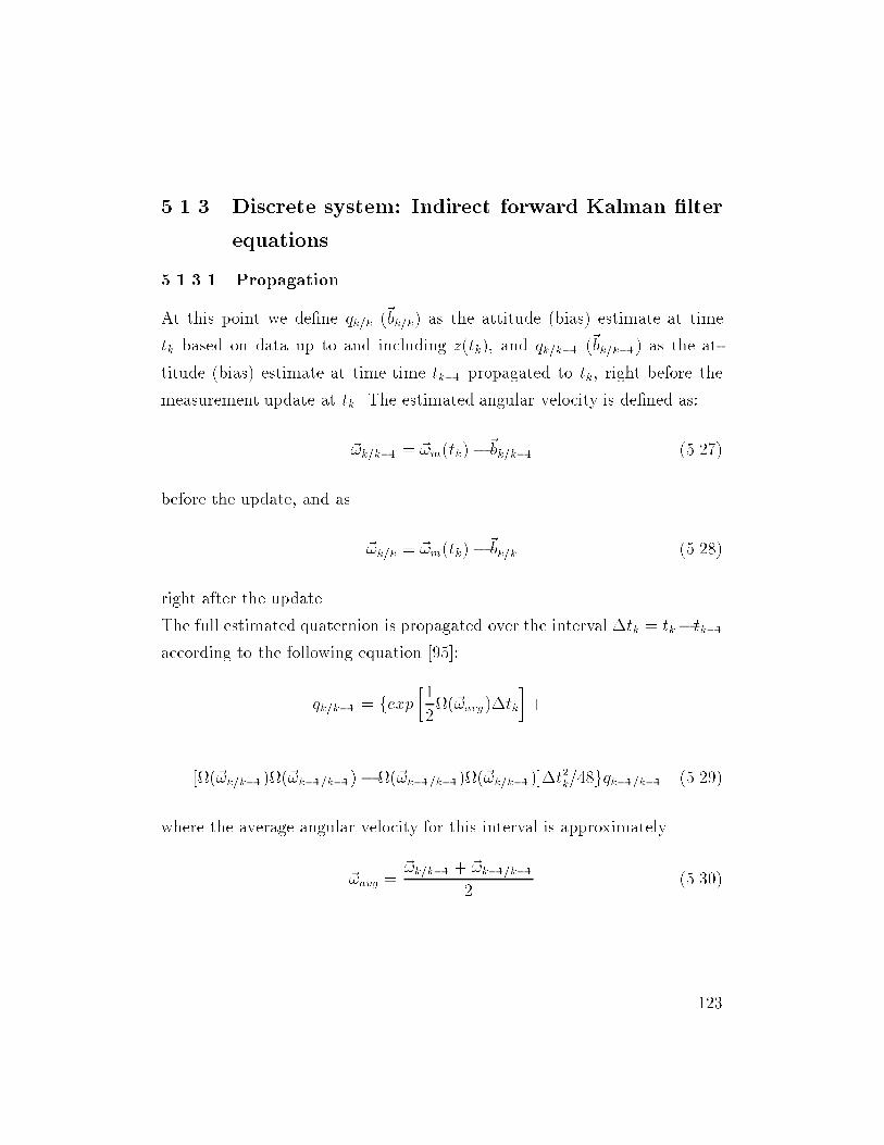
5.1.3 Discrete system: Indirect forward Kalman lter
equations
5.1.3.1 Propagation
At this point we dene qk=k (~bk=k) as the attitude (bias) estimate at time
tk based on data up to and including z(tk), and qk=k1 (~bk=k1) as the at-
titude (bias) estimate at time time tk1 propagated to tk, right before the
measurement update at tk. The estimated angular velocity is dened as:
~!k=k1 = ~!m(tk)~bk=k1 (5.27)
before the update, and as
~!k=k = ~!m(tk)~bk=k (5.28)
right after the update.
The full estimated quaternion is propagated over the interval tk = tk tk1
according to the following equation [95]:
qk=k1 = fexp1
2(~!avg)tk
+
[(~!k=k1)(~!k1=k1) (~!k1=k1)(~!k=k1)]t2k=48gqk1=k1 (5.29)
where the average angular velocity for this interval is approximately
~!avg =~!k=k1 + ~!k1=k1
2(5.30)
123
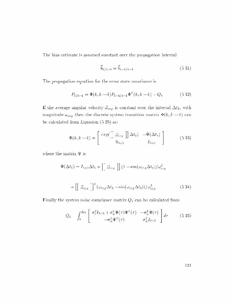
The bias estimate is assumed constant over the propagation interval
~bk=k1 = ~bk1=k1 (5.31)
The propagation equation for the error state covariance is
Pk=k1 = (k; k 1)Pk1=k1T (k; k 1) +Qk (5.32)
If the average angular velocity ~!avg is constant over the interval tk, with
magnitude !avg then the discrete system transition matrix (k; k 1) can
be calculated from Equation (5.25) as:
(k; k 1) =
24 exp(
hh~!avg
iitk) (tk)
033 I33
35 (5.33)
where the matrix is
(tk) = I33tk +hh
~!avgii(1 cos(!avgtk)=!
2avg
+hh
~!avgii2
(!avgtk sin(!avgtk))=!3avg (5.34)
Finally the system noise covariance matrix Qk can be calculated from
Qk =
Z tk
0
24 2rI33 + 2w( )
T ( ) 2w( )
2wT ( ) 2wI33
35 d (5.35)
124
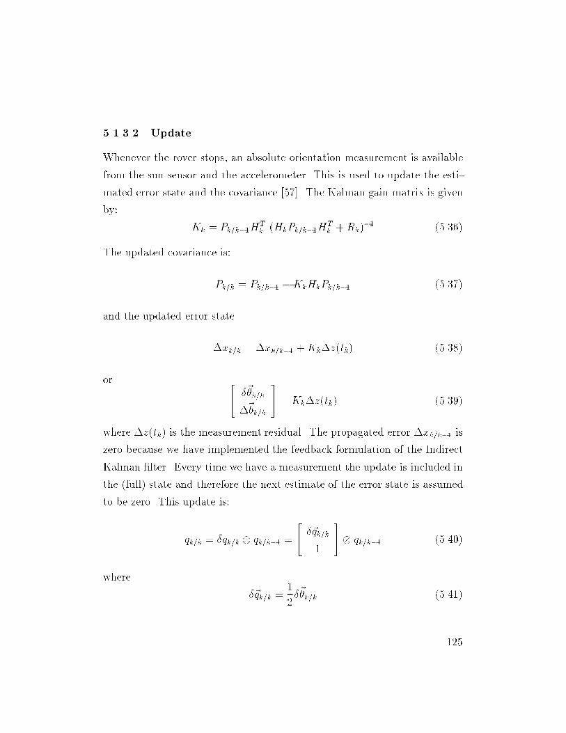
5.1.3.2 Update
Whenever the rover stops, an absolute orientation measurement is available
from the sun sensor and the accelerometer. This is used to update the esti-
mated error state and the covariance [57]. The Kalman gain matrix is given
by:
Kk = Pk=k1HTk (HkPk=k1H
Tk +Rk)
1 (5.36)
The updated covariance is:
Pk=k = Pk=k1 KkHkPk=k1 (5.37)
and the updated error state
xk=k = xk=k1 +Kkz(tk) (5.38)
or 24 ~k=k
~bk=k
35 = Kkz(tk) (5.39)
where z(tk) is the measurement residual. The propagated error xk=k1 is
zero because we have implemented the feedback formulation of the Indirect
Kalman lter. Every time we have a measurement the update is included in
the (full) state and therefore the next estimate of the error state is assumed
to be zero. This update is:
qk=k = qk=k qk=k1 =
24 ~qk=k
1
35 qk=k1 (5.40)
where
~qk=k =1
2~k=k (5.41)
125
and
~bk=k = ~bk=k1 +~bk=k (5.42)
5.1.3.3 Observation model
The attitude sensors considered here are the sun sensor and the triaxial ac-
celerometer; both are used when the rover is stopped. The rst one measures
the unit vector towards the sun and the second one provides the unit vec-
tor in the vertical direction. These measurements depend explicitly on the
attitude and not on the gyroscopes' biases. Let the observed vector in the
sensor frame be
pS(tk) = TS BA(q(tk))pI + ~np (5.43)
where pS is the measured unit vector in the sensor frame, pI is the reference
unit vector in the inertial frame (pointing in the direction of the sun for
example - we assume that it does not change signicantly for small time
intervals), TS B is the transformation matrix from the body frame to the
sensor frame, A(q(tk)) is the true orientation matrix of the robot at time tk,
q(tk) is the true attitude quaternion (qtrue) at time tk and ~np is the sensor
noise. If pS;k=k1 is the estimate of the measured unit vector at time tk and
is the matrix that projects the measurements on a plane perpendicular to
the sensor bore-sight, then the residual z(tk) can be written as:
z(tk) = (pS(tk) pS;k=k1) = (TS BA(q(tk))pI+~npTS BA(qk1=k)pI)
(5.44)
The true orientation matrix is
A(q(tk)) = A(~q(tk) qk=k1) = A(~q(tk))A(qk=k1) (5.45)
126
From Equation (5.6) we have:
A(~q(tk)) = (jq4(tk)j2~q T (tk) ~q(tk))I33+2~q(tk)~qT (tk)+2q4(tk)
hh~q(tk)
ii(5.46)
Using the small rotation angle approximations
q4(tk) ' 1 (5.47)
~q T (tk) ~q(tk) ' 0 (5.48)
~q(tk)~qT (tk) ' 033 (5.49)
we can write
A(~q(tk)) ' I33 + 2hh
~q(tk)ii
(5.50)
Substituting back in Equation (5.45) we get
A(q(tk)) ' (I33 + 2hh
~q(tk)ii)A(qk=k1) = (I33 +
hh~(tk)
ii)A(qk=k1)
(5.51)
Using this result in Equation (5.44) we have similar results to those in [83]:
z(tk) = (TS B
hh~(tk)
iiA(qk=k1)pI + ~np)
=
24 sx A(qk=k1)pI
sy A(qk=k1)pI
35 ~(tk) + ~np = hk=k1~(tk) + ~np (5.52)
where sx and sy are the unit vectors along the sensor axes. From the pre-
vious equation it is obvious that the observation model is non-linear and to
127
calculate the sensitivity (measurement) matrix we have to derive the par-
tial derivatives of z with respect to the estimated error states [56]. The
measurements are independent of gyro bias and thus:
Hk =@(z)
@(~)=hhk=k1 023
i(5.53)
5.1.4 Backward lter
In the ow chart shown in Figure 5.1 we see that the robot stops every time
the uncertainty grows beyond a preset threshold. Then the backward lter
is engaged and the last attitude estimate is propagated backwards in time.
This last estimate is precise because it is based on the absolute orientation
measurement acquired when the robot stopped. During the time instants
preceding stopping, the uncertainty grew considerably and the information
provided by the forward lter was of low quality. For this part of the trajec-
tory the backward lter is crucially needed. It uses the stored gyro values
and recalculates the orientation angles starting from a very precise initial
estimate. While the backward lter is close to its starting point it is able to
provide estimates of higher condence than those of the forward lter.
In order to derive the equations for the 3D backward Indirect Kalman
lter we start again from the equations of the system for the forward case:
_x = F x+G w (5.54)
z = H x+ v (5.55)
By dening
= T t (5.56)
128
where is the backward time variable and T = tk tkM is the time interval
of smoothing, the backward system equation can be derived from:
dx
d=
dx
dt
dt
d= _x (5.57)
ordxb
d= F xb G w (5.58)
Thus, Equation (5.25) for the backward system becomes:
d
dt
24 ~b
~bb
35 =
24
hh~!m
iiI33
033 033
3524 ~b
~bb
35+
24 I33 033
033 I33
3524 ~nr
~nw
35
(5.59)
and from this the discrete backward system transition matrix is calculated
to be:
(b; k 1; k) =
24 exp(
hh~!avg
iitk) b(tk)
033 I33
35 (5.60)
with
b(tk) = I33tk hh
~!avgii
(1 cos(!avgtk)=!2avg +
hh~!avg
ii2(!avgtk sin(!avgtk))=!
3avg (5.61)
Instead of Equation (5.29) the quaternion estimate is propagated according
to:
qb;k1=k1 = fexp[1
2(~!avg)tk]+
129
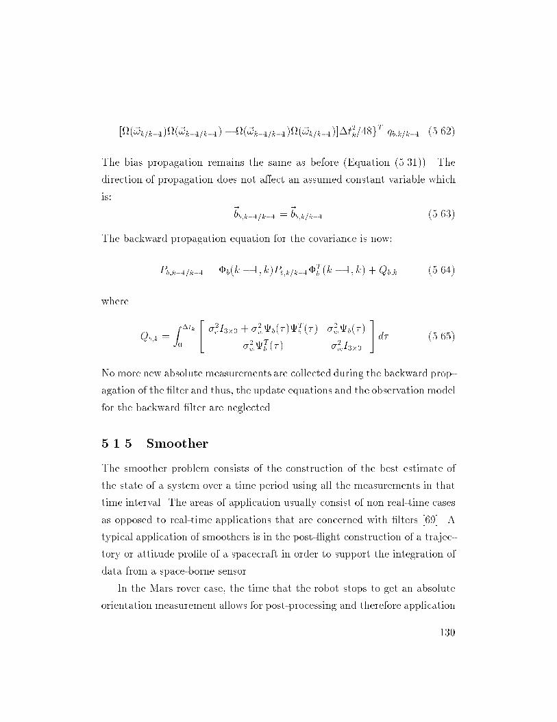
[(~!k=k1)(~!k1=k1) (~!k1=k1)(~!k=k1)]t2k=48g
T qb;k=k1 (5.62)
The bias propagation remains the same as before (Equation (5.31)). The
direction of propagation does not aect an assumed constant variable which
is:
~bb;k1=k1 = ~bb;k=k1 (5.63)
The backward propagation equation for the covariance is now:
Pb;k1=k1 = b(k 1; k)Pb;k=k1Tb (k 1; k) +Qb;k (5.64)
where
Qb;k =
Z tk
0
24 2rI33 + 2wb( )
Tb ( ) 2wb( )
2wTb ( ) 2wI33
35 d (5.65)
No more new absolute measurements are collected during the backward prop-
agation of the lter and thus, the update equations and the observation model
for the backward lter are neglected.
5.1.5 Smoother
The smoother problem consists of the construction of the best estimate of
the state of a system over a time period using all the measurements in that
time interval. The areas of application usually consist of non real-time cases
as opposed to real-time applications that are concerned with lters [69]. A
typical application of smoothers is in the post- ight construction of a trajec-
tory or attitude prole of a spacecraft in order to support the integration of
data from a space-borne sensor.
In the Mars rover case, the time that the robot stops to get an absolute
orientation measurement allows for post-processing and therefore application
130
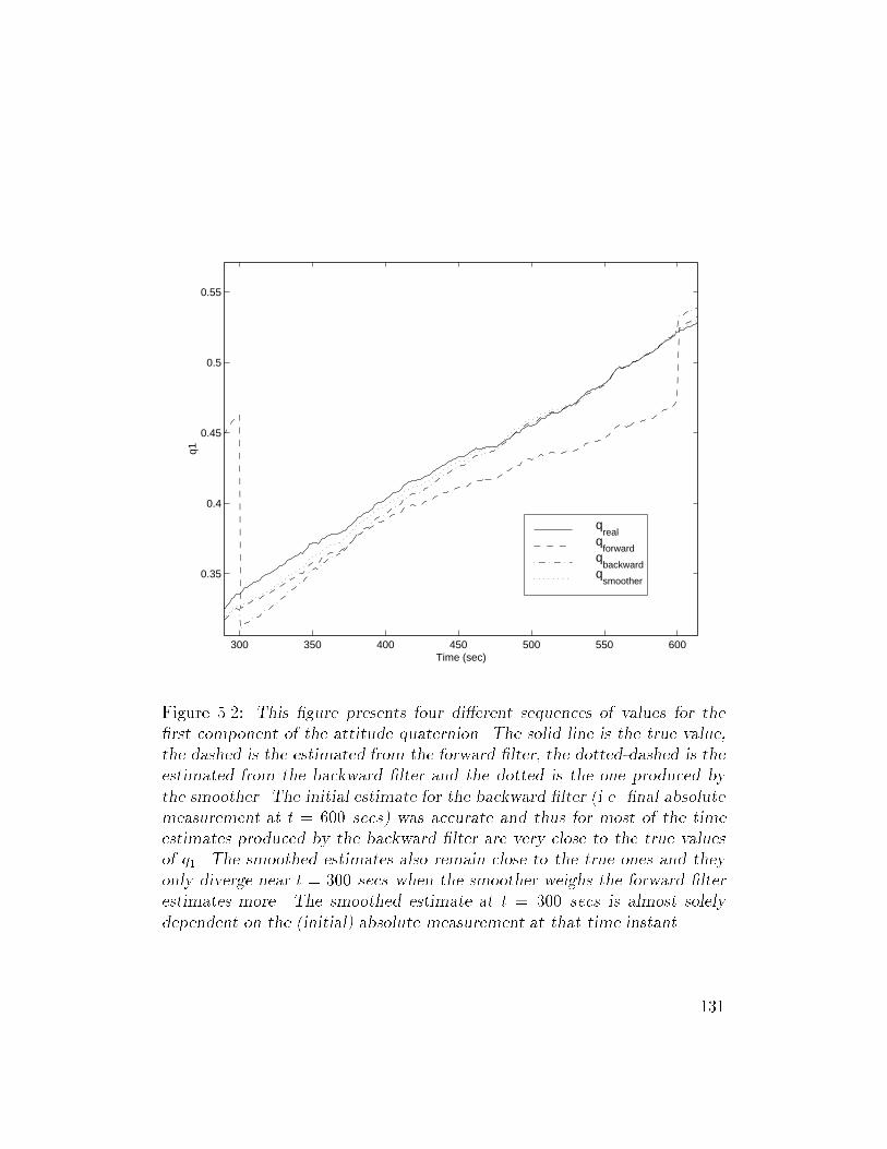
300 350 400 450 500 550 600
0.35
0.4
0.45
0.5
0.55
q1
Time (sec)
qreal
qforward
qbackward
qsmoother
Figure 5.2: This gure presents four dierent sequences of values for the
rst component of the attitude quaternion. The solid line is the true value,
the dashed is the estimated from the forward lter, the dotted-dashed is the
estimated from the backward lter and the dotted is the one produced by
the smoother. The initial estimate for the backward lter (i.e. nal absolute
measurement at t = 600 secs) was accurate and thus for most of the time
estimates produced by the backward lter are very close to the true values
of q1. The smoothed estimates also remain close to the true ones and they
only diverge near t = 300 secs when the smoother weighs the forward lter
estimates more. The smoothed estimate at t = 300 secs is almost solely
dependent on the (initial) absolute measurement at that time instant.
131
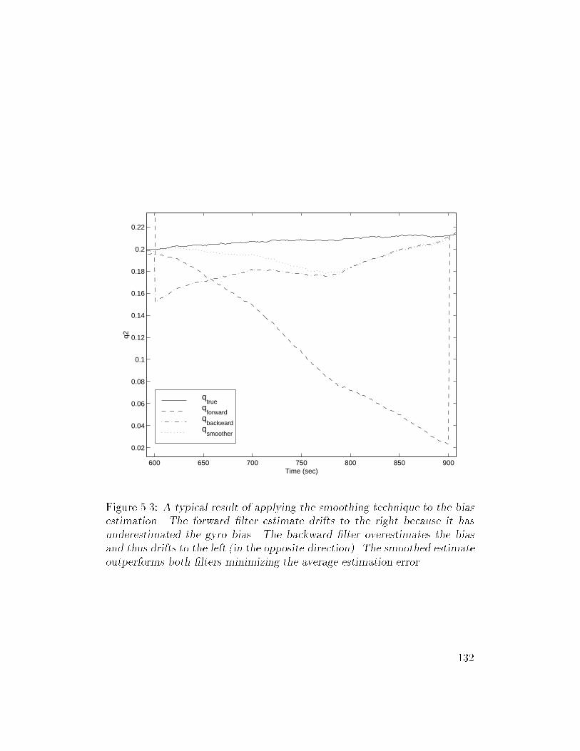
600 650 700 750 800 850 900
0.02
0.04
0.06
0.08
0.1
0.12
0.14
0.16
0.18
0.2
0.22
q2
Time (sec)
qtrue
qforward
qbackward
qsmoother
Figure 5.3: A typical result of applying the smoothing technique to the bias
estimation. The forward lter estimate drifts to the right because it has
underestimated the gyro bias. The backward lter overestimates the bias
and thus drifts to the left (in the opposite direction). The smoothed estimate
outperforms both lters minimizing the average estimation error.
132
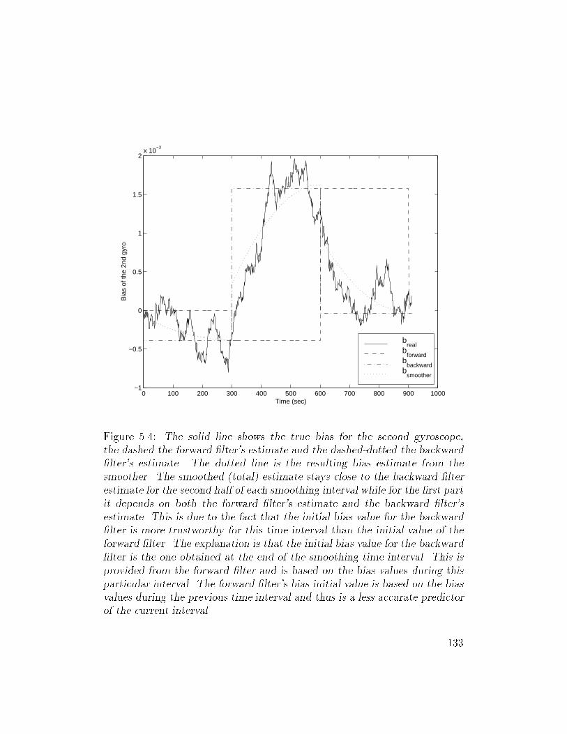
0 100 200 300 400 500 600 700 800 900 1000−1
−0.5
0
0.5
1
1.5
2x 10
−3
Bia
s of
the
2nd
gyro
Time (sec)
breal
bforward
bbackward
bsmoother
Figure 5.4: The solid line shows the true bias for the second gyroscope,
the dashed the forward lter's estimate and the dashed-dotted the backward
lter's estimate. The dotted line is the resulting bias estimate from the
smoother. The smoothed (total) estimate stays close to the backward lter
estimate for the second half of each smoothing interval while for the rst part
it depends on both the forward lter's estimate and the backward lter's
estimate. This is due to the fact that the initial bias value for the backward
lter is more trustworthy for this time interval than the initial value of the
forward lter. The explanation is that the initial bias value for the backward
lter is the one obtained at the end of the smoothing time interval. This is
provided from the forward lter and is based on the bias values during this
particular interval. The forward lter's bias initial value is based on the bias
values during the previous time interval and thus is a less accurate predictor
of the current interval.
133
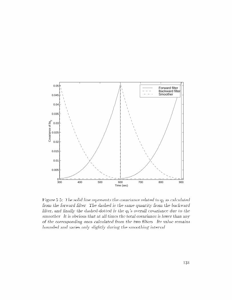
300 400 500 600 700 800 9000
0.005
0.01
0.015
0.02
0.025
0.03
0.035
0.04
0.045
0.05
Cov
aria
nce
of δ
q 2
Time (sec)
Forward filterBackward filterSmoother
Figure 5.5: The solid line represents the covariance related to q2 as calculated
from the forward lter. The dashed is the same quantity from the backward
lter, and nally the dashed-dotted is the q2's overall covariance due to the
smoother. It is obvious that at all times the total covariance is lower than any
of the corresponding ones calculated from the two lters. Its value remains
bounded and varies only slightly during the smoothing interval.
134
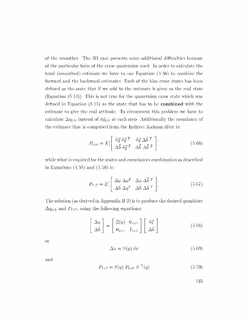
of the smoother. The 3D case presents some additional diculties because
of the particular form of the error quaternion used. In order to calculate the
total (smoothed) estimate we have to use Equation (4.56) to combine the
forward and the backward estimates. Each of the bias error states has been
dened as the state that if we add to the estimate it gives us the real state
(Equation (5.14)). This is not true for the quaternion error state which was
dened in Equation (5.15) as the state that has to be combined with the
estimate to give the real attitude. To circumvent this problem we have to
calculate qk=k instead of ~qk=k at each step. Additionally the covariance of
the estimate that is computed from the Indirect Kalman lter is:
P66 = E[
24 ~q ~q T ~q ~b T
~b ~q T ~b ~b T
35] (5.66)
while what is required for the states and covariances combination as described
in Equations (4.55) and (4.56) is:
P77 = E[
24 q qT q ~b T
~b qT ~b ~b T
35] (5.67)
The solution (as derived in Appendix B.2) is to produce the desired quantities
qk=k and P77, using the following equations:
24 q
~b
35 =
24 (q) 033
043 I33
3524 ~q
~b
35 (5.68)
or
x = S(q) x (5.69)
and
P77 = S(q) P66 ST (q) (5.70)
135
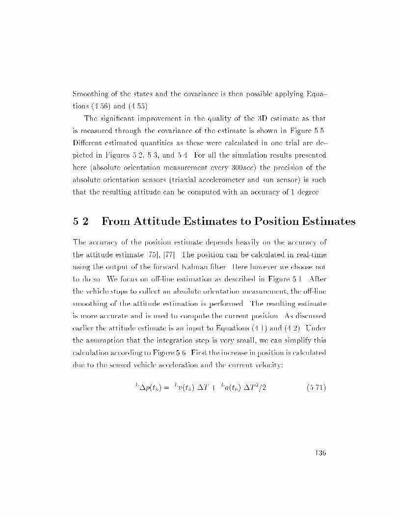
Smoothing of the states and the covariance is then possible applying Equa-
tions (4.56) and (4.55).
The signicant improvement in the quality of the 3D estimate as that
is measured through the covariance of the estimate is shown in Figure 5.5.
Dierent estimated quantities as these were calculated in one trial are de-
picted in Figures 5.2, 5.3, and 5.4. For all the simulation results presented
here (absolute orientation measurement every 300sec) the precision of the
absolute orientation sensors (triaxial accelerometer and sun sensor) is such
that the resulting attitude can be computed with an accuracy of 1 degree.
5.2 From Attitude Estimates to Position Estimates
The accuracy of the position estimate depends heavily on the accuracy of
the attitude estimate [75], [77]. The position can be calculated in real-time
using the output of the forward Kalman lter. Here however we choose not
to do so. We focus on o-line estimation as described in Figure 5.1. After
the vehicle stops to collect an absolute orientation measurement, the o-line
smoothing of the attitude estimation is performed. The resulting estimate
is more accurate and is used to compute the current position. As discussed
earlier the attitude estimate is an input to Equations (4.1) and (4.2). Under
the assumption that the integration step is very small, we can simplify this
calculation according to Figure 5.6. First the increase in position is calculated
due to the sensed vehicle acceleration and the current velocity:
Lp(tk) =Lv(tk) T + La(tk) T
2=2 (5.71)
136
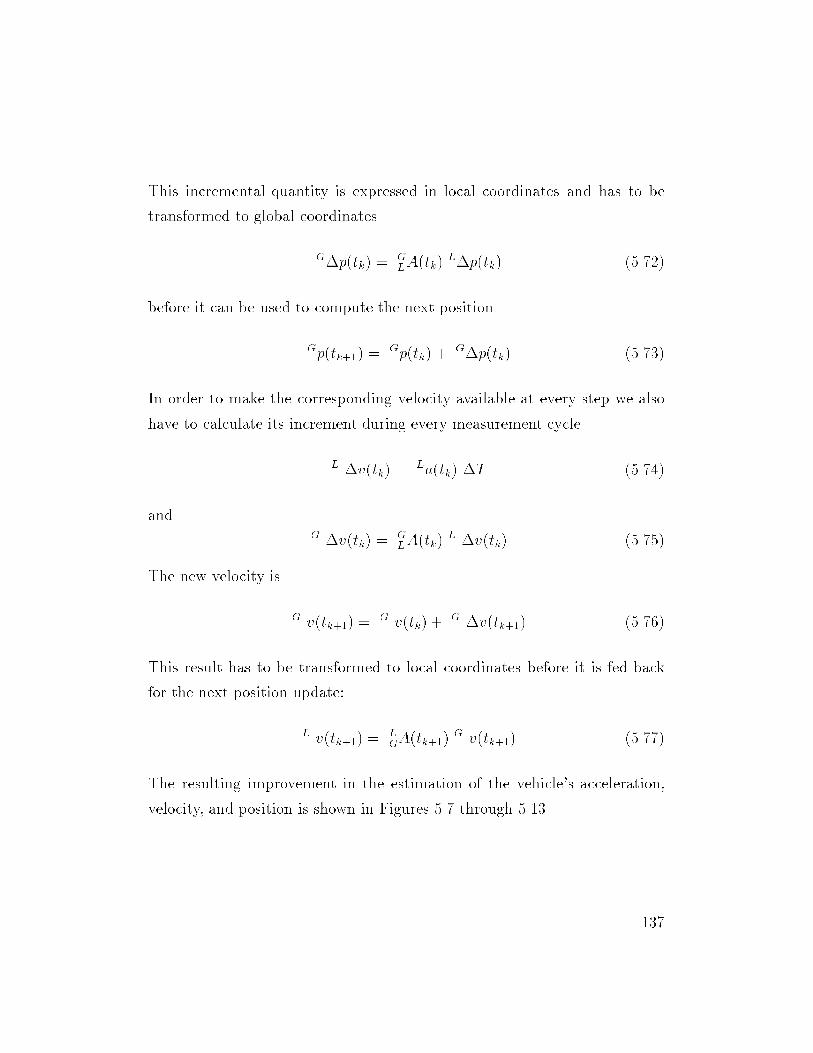
This incremental quantity is expressed in local coordinates and has to be
transformed to global coordinates
Gp(tk) =GLA(tk)
Lp(tk) (5.72)
before it can be used to compute the next position
Gp(tk+1) =Gp(tk) +
Gp(tk) (5.73)
In order to make the corresponding velocity available at every step we also
have to calculate its increment during every measurement cycle.
L v(tk) =La(tk) T (5.74)
andG v(tk) =
GLA(tk)
L v(tk) (5.75)
The new velocity is
G v(tk+1) =G v(tk) +
G v(tk+1) (5.76)
This result has to be transformed to local coordinates before it is fed back
for the next position update:
L v(tk+1) =LGA(tk+1)
G v(tk+1) (5.77)
The resulting improvement in the estimation of the vehicle's acceleration,
velocity, and position is shown in Figures 5.7 through 5.13.
137
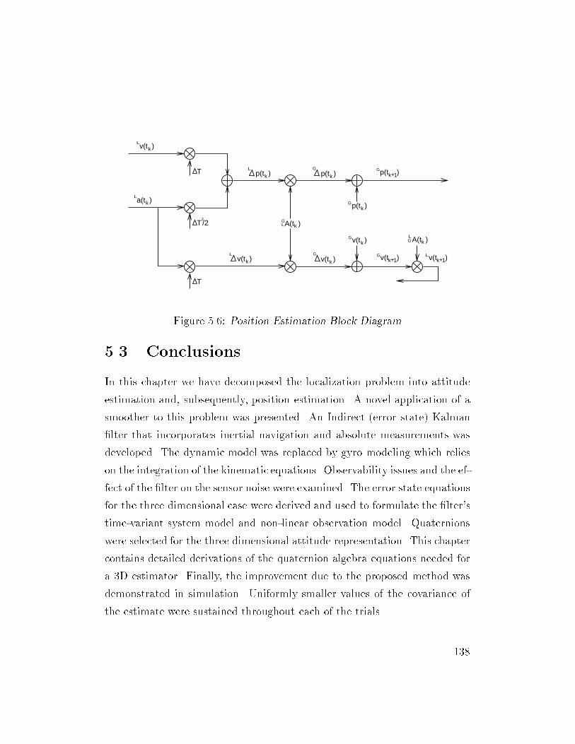
p(t )k
L
v(t )kL
a(t )kL
Gp(t )k
Gp(t )k
v(t )k
Gv(t )k
L
T
T
T/22
v(t )kG
k+1v(t )G
p(t )k+1G
Lk+1v(t )
LG
kA(t )
kA(t )LG
Figure 5.6: Position Estimation Block Diagram
5.3 Conclusions
In this chapter we have decomposed the localization problem into attitude
estimation and, subsequently, position estimation. A novel application of a
smoother to this problem was presented. An Indirect (error state) Kalman
lter that incorporates inertial navigation and absolute measurements was
developed. The dynamic model was replaced by gyro modeling which relies
on the integration of the kinematic equations. Observability issues and the ef-
fect of the lter on the sensor noise were examined. The error state equations
for the three dimensional case were derived and used to formulate the lter's
time-variant system model and non-linear observation model. Quaternions
were selected for the three dimensional attitude representation. This chapter
contains detailed derivations of the quaternion algebra equations needed for
a 3D estimator. Finally, the improvement due to the proposed method was
demonstrated in simulation. Uniformly smaller values of the covariance of
the estimate were sustained throughout each of the trials.
138
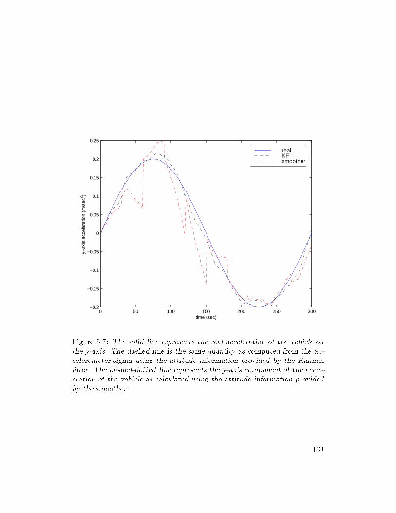
0 50 100 150 200 250 300−0.2
−0.15
−0.1
−0.05
0
0.05
0.1
0.15
0.2
0.25
y−ax
is a
ccel
erat
ion
(m/s
ec2 )
time (sec)
realKFsmoother
Figure 5.7: The solid line represents the real acceleration of the vehicle on
the y-axis. The dashed line is the same quantity as computed from the ac-
celerometer signal using the attitude information provided by the Kalman
lter. The dashed-dotted line represents the y-axis component of the accel-
eration of the vehicle as calculated using the attitude information provided
by the smoother.
139
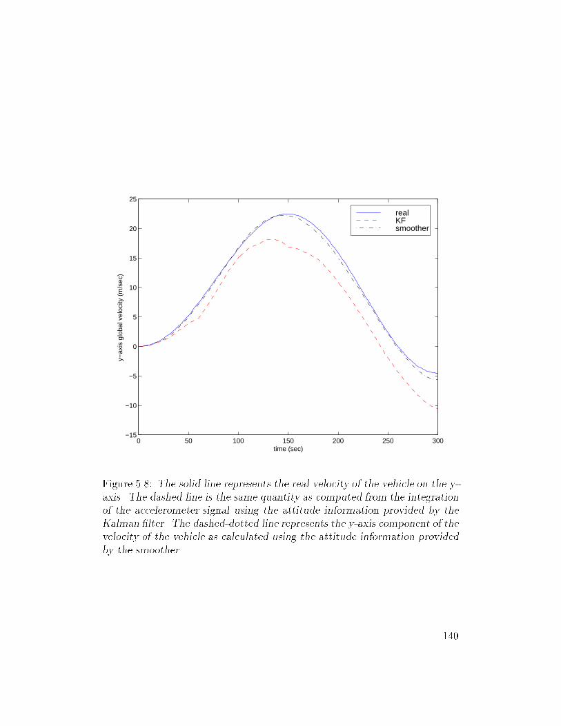
0 50 100 150 200 250 300−15
−10
−5
0
5
10
15
20
25
y−ax
is g
loba
l vel
ocity
(m
/sec
)
time (sec)
realKFsmoother
Figure 5.8: The solid line represents the real velocity of the vehicle on the y-
axis. The dashed line is the same quantity as computed from the integration
of the accelerometer signal using the attitude information provided by the
Kalman lter. The dashed-dotted line represents the y-axis component of the
velocity of the vehicle as calculated using the attitude information provided
by the smoother.
140
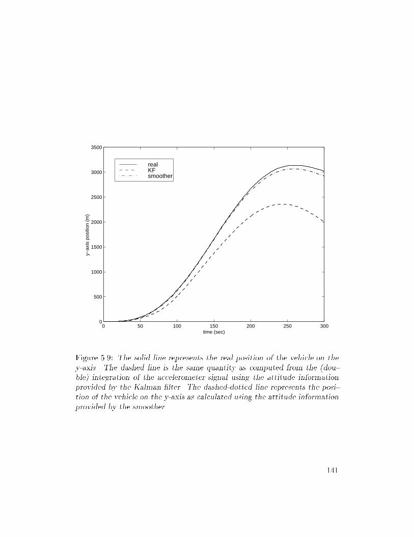
0 50 100 150 200 250 3000
500
1000
1500
2000
2500
3000
3500
y−ax
is p
ositi
on (
m)
time (sec)
realKFsmoother
Figure 5.9: The solid line represents the real position of the vehicle on the
y-axis. The dashed line is the same quantity as computed from the (dou-
ble) integration of the accelerometer signal using the attitude information
provided by the Kalman lter. The dashed-dotted line represents the posi-
tion of the vehicle on the y-axis as calculated using the attitude information
provided by the smoother.
141
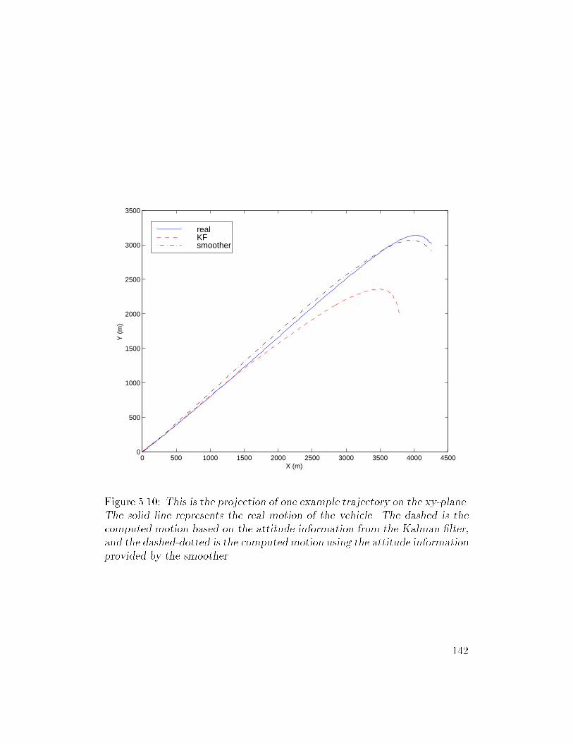
0 500 1000 1500 2000 2500 3000 3500 4000 45000
500
1000
1500
2000
2500
3000
3500
X (m)
Y (
m)
realKFsmoother
Figure 5.10: This is the projection of one example trajectory on the xy-plane.
The solid line represents the real motion of the vehicle. The dashed is the
computed motion based on the attitude information from the Kalman lter,
and the dashed-dotted is the computedmotion using the attitude information
provided by the smoother.
142
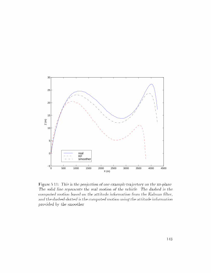
0 500 1000 1500 2000 2500 3000 3500 4000 4500−5
0
5
10
15
20
25
30
X (m)
Z (
m)
realKFsmoother
Figure 5.11: This is the projection of one example trajectory on the xz-plane.
The solid line represents the real motion of the vehicle. The dashed is the
computed motion based on the attitude information from the Kalman lter,
and the dashed-dotted is the computedmotion using the attitude information
provided by the smoother.
143
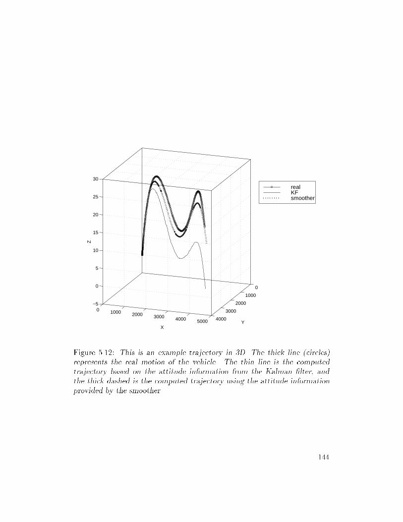
0 1000 2000 3000 4000 5000
0
1000
2000
3000
4000
−5
0
5
10
15
20
25
30
YX
Z
realKFsmoother
Figure 5.12: This is an example trajectory in 3D. The thick line (circles)
represents the real motion of the vehicle. The thin line is the computed
trajectory based on the attitude information from the Kalman lter, and
the thick dashed is the computed trajectory using the attitude information
provided by the smoother.
144
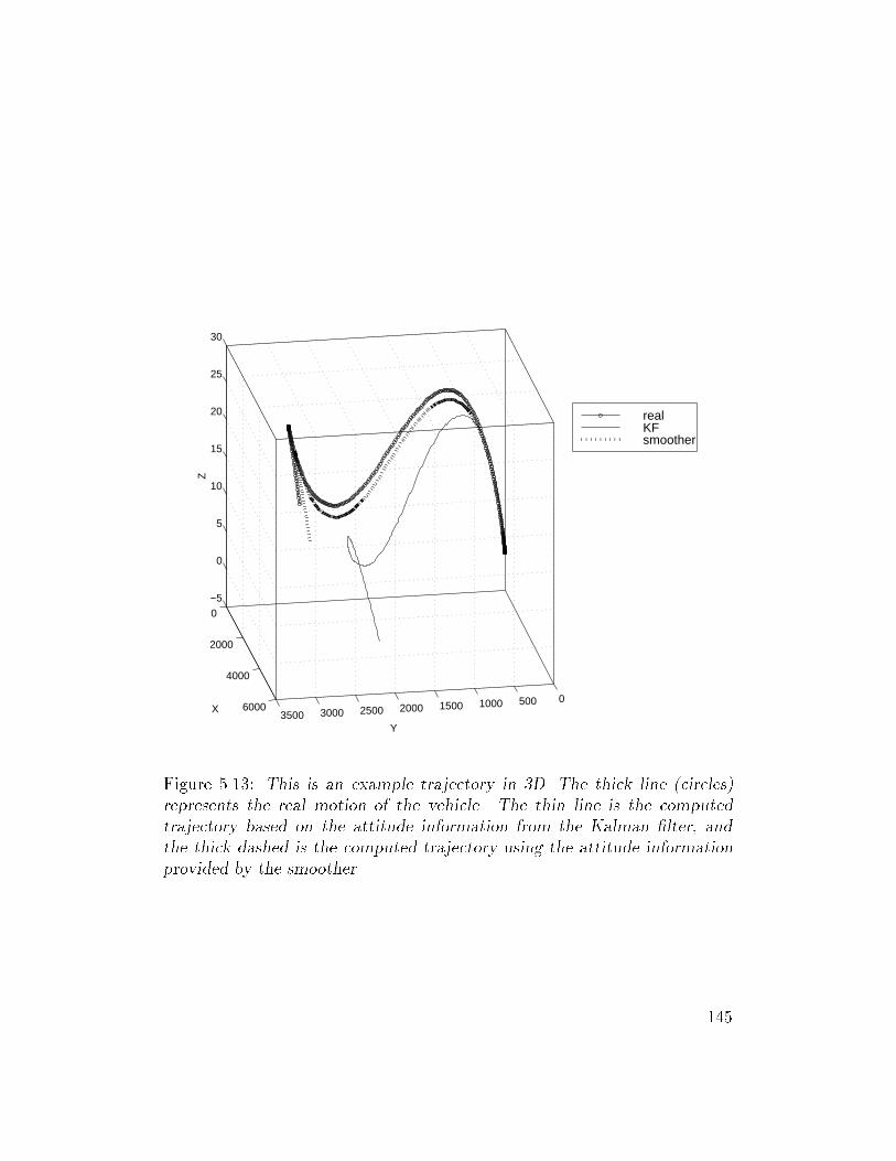
0
2000
4000
60000500100015002000250030003500
−5
0
5
10
15
20
25
30
Y
X
Z
realKFsmoother
Figure 5.13: This is an example trajectory in 3D. The thick line (circles)
represents the real motion of the vehicle. The thin line is the computed
trajectory based on the attitude information from the Kalman lter, and
the thick dashed is the computed trajectory using the attitude information
provided by the smoother.
145
5.4 Extensions
This technique is not limited to the case of Mars rovers. It can be used for
smoothing the orientation estimates and thus improving the localization ac-
curacy for various robotic platforms that carry an equivalent set of sensors.
We cite below a few examples of robotic systems that lack attitude observ-
ability during certain time intervals.
i) Vision, encoders (and gyros) - Outdoor environment: In this scenario
a vision system is used to dene the orientation of the vehicle by calculating
the bearing from a distant object (e.g. the top of a mountain or a build-
ing). While this object is occluded, the robot relies on the encoders (and/or
gyroscopes) to estimate its orientation. When the line of sight is cleared, a
new absolute measurement of the orientation is available and the previous
estimates can be smoothed based on it.
ii) Compass, encoders (and gyros) - Outdoor environment: In this case
the compass signal becomes unreliable when the vehicle moves close to large
metallic objects (e.g. cars) or areas with non-negligible magnetic eld in-
duced by electric wires. The quality of the orientation estimates is poor for
this part of the trajectory. It is substantially improved when the vehicle
leaves this area. Back propagation of the new reliable absolute orientation
measurement will reduce the previous attitude uncertainty. Updating of the
position estimates is then possible.
iii) Encoders (and gyros) - Indoor environment: Here the absolute orien-
tation information is drawn from the structure of the environment. A robot
that moves along a straight wall is able to re-orient every time it aligns itself
with respect to the wall (in a parallel or perpendicular to the wall direction).
The corrected orientation can be used to smooth the previous attitude esti-
mates and enhance the quality of the position tracking.
146
iv) Absolute positioning sensors and INS and/or odometric sensors: In
the previous cases the objective was to apply the presented smoothing tech-
nique to orientation estimates and subsequently to improve the quality of
the position tracking. Another category of problems that this method can
be extended to is position smoothing. In recent years, GPS (Global Posi-
tioning System) based localization has become popular. In addition, other
methods that use the distance from natural or articial landmarks (beacons
instead of satellites) to triangulate the absolute position of the vehicle, have
shown immense potential. Global vision can also be used to globally localize
a vehicle, mainly for indoor applications. These systems fail when the signals
they rely on become unobservable. In the case of GPS for example, this can
happen when the vehicle is in the vicinity of large buildings or indoors. A
similar situation is when one of the (at least three) landmarks required for
triangulation is occluded or cannot be detected, or when the vehicle is out
of the eld of view of the global camera(s). For these parts of the trajectory,
the robots have to rely on odometric and/or INS sensors. When the signal(s)
is (are) available again, the whole trajectory (intermediate positions) can be
reconstructed precisely using a smoother. The resulting accurate path is
particularly useful when mapping is performed or when the robot senses its
environment for certain cues. In the second case the robot uses pictures or
video of the area to locate items of interest (e.g. a bomb or an injured per-
son), or deploys metal detectors to reveal the position of a mine, or radiation
detectors to investigate radiation leakages, to mention a few examples.
147
Chapter 6
Collective Localization for a Group of Mobile
Robots
6.1 Introduction
Many robotic applications require that robots work in collaboration in order
to perform a certain task [27], [54], [64]. Most existing localization approaches
have been developed for the case of a single robot. Even when a group of,
say M , robots is considered, the group localization problem is usually re-
solved by independently solving M pose estimation problems. Each robot
estimates its position based on its individual experience (proprioceptive and
exteroceptive sensor measurements). Knowledge from the dierent entities
of the team is not combined and each member must rely on its own resources
(sensing and processing capabilities). This is a relatively simple approach
since it avoids dealing with the complicated problem of fusing information
from a large number of independent and interdependent sources. On the
other hand, a more coordinated schema for localization has a number of ad-
vantages that can compensate for the added complexity.
First let us consider the case of a homogeneous group of robots. As
we mentioned earlier, robotic sensing modalities suer from uncertainty and
148
noise. When a number of robots equipped with the same sensors detect a
particular feature of the environment, such as a door, or measure a charac-
teristic property of the area, such as the local vector of the earth's magnetic
eld, a number of independent measurements originating from the dierent
members of the group is collected. Properly combining all this information
will result in a single estimate of increased accuracy and reduced uncertainty.
A better estimate of the position and orientation of a landmark can drasti-
cally improve the outcome of the localization process and thus this group of
robots can benet from this collaboration schema.
The advantages stemming from the exchange of information among the
members of a group are more crucial in the case of heterogeneous robotic
colonies. When a team of robots is composed of dierent platforms carrying
dierent proprioceptive and exteroceptive sensors and thus having dier-
ent capabilities for self-localization, the quality of the localization estimates
will vary signicantly across the individual members. For example, a robot
equipped with a laser scanner and expensive INS/GPS modules will outper-
form another member that must rely on wheel encoders and cheap sonars
for its localization needs. Communication and ow of information among
the members of the group constitutes a form of sensor sharing and can im-
prove the overall positioning accuracy. In fact, as will be evident later, if
each robot could sense and communicate with its colleagues at all times then
every member of the group would have less uncertainty about its position
than the robot with the best localization results (if it were to localize itself
without communicating with the rest of the group).
In the following section we will refer to previous approaches to the collab-
oration of robots in order to perform localization and we will state the main
dierences between these approaches and the collective localization scheme.
149
6.2 Previous Approaches
An example of a system that is designed for cooperative localization is pre-
sented in [48]. The authors acknowledge that dead-reckoning is not reliable
for long traverses due to the error accumulation and introduce the concept
of \portable landmarks". A group of robots is divided into two teams in
order to perform cooperative positioning. At each time instant, one team
is in motion while the other remains stationary and acts as a landmark. In
the next phase the roles of the teams are reversed and this process continues
until both teams reach the target. This method can work in unknown envi-
ronments and the conducted experiments suggest accuracies of 0.4% for the
position estimate and 1 degree for the orientation [47]. Improvements over
this system and optimum motion strategies are discussed in [46].
A similar realization is presented in [67], [68]. The authors deal with the
problem of exploration of an unknown environment using two mobile robots.
In order to reduce the odometric error, one robot is equipped with a camera
tracking system that allows it to determine its relative position and orienta-
tion with respect to a second robot carrying a helix target pattern and acting
as a portable landmark.
Both previous approaches have the following limitations: (a) Only one
robot (or team) is allowed to move at any given time, and (b) The two
robots (or teams) must maintain visual contact at all times. Although prac-
tices like those previously mentioned can be supported within the collective
localization framework (Section 6.7), the key dierence is that it provides a
solution to the most general case where all the robots in the group can move
simultaneously while continuous visual contact is not required.
In order to treat the group localization problem, we begin from the rea-
sonable assumptions that the robots within the group can communicate with
each other (at least 1-to-1 communication) and carry two types of sensors:
150
1. Proprioceptive sensors that record the self motion of each robot and allow
for position tracking, 2. Exteroceptive sensors that monitor the environ-
ment for (a) (static) features and identities of the surroundings of the robot
to be used in the localization process, and (b) other robots (treated as dy-
namic features). The goal is to integrate measurements collected by dierent
robots and achieve localization across all the robotic platforms constituting
the group.
The key idea for performing collective localization is that the group of
robots must be viewed as one entity - the \group organism" - with multiple
\limbs" (the individual robots in the group) and multiple virtual \joints"
visualized as connecting each robot with every other member of the team
[79], [81]. The virtual \joints" provide 3 degrees of freedom (x;y;)1
and thus allow the \limbs" to move in every direction within a plane with-
out any limitations. Considering this perspective, the \group organism" has
access to a large number of sensors such as encoders, gyroscopes, cameras
etc. In addition, it \spreads" itself across a large area and thus it can col-
lect far more rich and diverse exteroceptive information than a single robot.
When one robot detects another member of the team and measures its rel-
ative pose, it is equivalent to the \group organism's" joints measuring the
relative displacement of these two \limbs". When two robots communicate
for information exchange, this can be seen as the \group organism" allowing
information to travel back and forth from its \limbs". This information can
be fused by a centralized processing unit and provide improved localization
results for all the robots in the group. At this point we note that a realization
of a two-member \group organism" would resemble the multiple degree of
freedom robot with compliant linkage, which was implemented by J. Boren-
stein [8], [9], [10], and it has been shown to improve localization accuracy.
16 dof in a 3 dimensional space of motion.
151
The main drawback of addressing the cooperative localization problem
as an information combination problem within a single entity (\group or-
ganism") is that it requires centralized processing and communication. The
solution would be to attempt to decentralize the sensor fusion within the
group. The collective localization approach uses the previous analogy as its
starting point and treats the processing and communication needs of the
group in a distributed fashion. This is intuitively desired; since the sensing
modalities of the group are distributed, so should be the processing modules.
In order to deal with the cross-correlation terms (localization interdepen-
dencies) that can alter the localization result (Section 6.3), the data processed
during each collective localization session must be propagated among all the
robots in the group. While this can happen instantly in groups of 2 robots,
in Section 6.4 we will show how this problem can be treated by reformulating
the collective localization approach so it can be applied in groups of 3 or more
robots.
6.3 Group Localization Interdependencies
In order to examine the eect of the interdependencies in the group local-
ization process we study the simple case of two robots constrained to move
in a single dimension and capable of exchanging positioning data. Every
time the two robots meet they have available two independent estimates
of their position. One is the estimate based on their own sensors xA()
(or xB()) and the other is derived from the measurement of their relative
position with respect to the other robot xA(meas) = xA;B + xB() (or
xB(meas) = xB;A+ xA()). The uncertainty of this additional estimate is
152
expressed by its covariance matrix PxA(meas)2 and it can be calculated by the
following equation:
PxA(meas) = PxA;B + PxB() = R + PxB() (6.1)
where:
R = PxA;B = EhnxA;Bn
TxA;B
i(6.2)
is the covariance matrix of the relative position measurement and its value
depends on the noise nxA;B associated with this measurement. From Equa-
tion (6.1), it is obvious that the quality of the additional estimate xA(meas)
depends on the quality of the relative position measurement xA;B and the
position estimate of robot B xB(). Small values of PxA(meas) require precise
localization of robot B (small values of PxB()) and an accurate relative po-
sition measurement (small values of PxA;B ). The two estimates xA() and
xA(meas), assuming that they are independent, can be combined as:
P1xA(+)= P1xA() + P1xA(meas) (6.3)
P1xA(+)xA(+) = P1xA() xA() + P1xA(meas) xA(meas) (6.4)
The previous equation expresses that the location of robot A is the weighted
average of where robot A itself believes it is and where robot B believes that
robot A is.
This combination of positioning information between two robots is valid
only when the robots meet for the rst time. If they meet again later, the
independence assumption is not valid anymore. The new propagated esti-
mates contain information exchanged during their previous rendezvous that
2For this one-dimensional case the covariance matrix is a scalar. Its one element is the
variance of the position estimate.
153
is now shared by both robots.3 The eect of this is explained in the following
numerical example:
Example 1: In this one-dimensional case, let us assume that robots
A and B started from the same point and moved (probably with dierent
speeds) along the same direction for some distance and then meet for the
rst time. In the mean time, the initial uncertainties for A and B have been
propagated and let us assume that their values have become PA(k) = 4 for
A and PB(k) = 4 for B4. In order to simplify the calculations, let us also
assume that the relative position measurement is almost perfect (zero uncer-
tainty associated with it). Applying Equation (6.3), the result of combining
these two independent sources of information would be P+A (k) = P+
B (k) = 2.
The robots move again and we assume that their uncertainty has in-
creased by PA(k; k+1) = PB(k; k+1) = 8. Then each of them will have
total uncertainty PA(k + 1) = P+A (k) +PA(k; k + 1) = 10 and PB(k + 1) =
P+B (k) + PB(k; k + 1) = 10. If the two robots meet again and we as-
sume (falsely) that their current estimates are independent, then their up-
dated covariance estimates according to Equation (6.3) would be: P+A (k +
1) = P+B (k + 1) = 5, which is over-optimistic. The reason is that the
independent part of information now is the one due to the motion after
the rst rendezvous and the associated uncertainty is PA(k; k + 1) and
PB(k; k + 1). Therefore, it is only legitimate to combine these last two
quantities and infer that due to the exchange of information between the
two robots the uncertainty associated with the last part of their motion is
3Another pathological situation would be if one or both of robots A and B which have
initially met, subsequently meet other robots C and D which have no knowledge of A and
B having met in the past. If C and D meet subsequently, their position estimates are not
independent and any exchange of information will produce levels of uncertainty that are
over-optimistic.4If the dimensions of x are meters (m) then the dimensions of the position covariance
matrices are m2.
154
updated to P+A (k; k +1) = P+
B (k; k +1) = 4. The overall position uncer-
tainty would now be: P+A (k + 1) = P+
A (k) + P+A (k; k + 1) = P+
B (k + 1) =
P+B (k) + P+
B (k; k + 1) = 2 + 4 = 6 > 5.
It is obvious that if the cross-correlation terms are not considered prop-
erly in the formulation of the localization information fusion, the resulting
positioning estimates will not be realistic. In the extreme case, if every time
the two robots have moved innitesimal distance they take another snapshot
of each other, their position uncertainty will decrease exponentially (becom-
ing almost half of its previous value during each update).
6.4 Problem Statement
We state the following assumptions:
1. A group of M independent robots move in an N dimensional space.
The motion of each robot is described by its own linear or non-linear
equations of motion,
2. Each robot carries proprioceptive and exteroceptive sensing devices in
order to propagate and update its own position estimate. The mea-
surement equations can dier from robot to robot depending on the
sensors used,
3. Each robot carries exteroceptive sensors that allow it to detect and
identify other robots moving in its vicinity and measure their respective
displacement (relative position and orientation),
4. All the robots are equipped with communication devices that allow
exchange of information within the group.
155
The problem is to determine a principled way to exploit the information
exchanged during the interactions among members of a group taking un-
der consideration possible independencies and interdependencies. It is also
within our focus to formulate the problem in such a way that it will allow
for distributed processing with minimal communication requirements. As we
will see in Sections 6.5 and 6.6, communication among the robots is only nec-
essary during the update cycle of collective localization; that is, only when
two robots meet.
As we mentioned before, our starting point is to consider this group of
robots as a single centralized system composed of each and every individual
robot moving in the area and capable of sensing and communicating with
the rest of the group. In this centralized approach, the motion of the group
is described in an N M -dimensional space and can be estimated by apply-
ing Kalman ltering techniques. The goal now is to treat the Kalman lter
equations of the centralized system so as to distribute the estimation process
among M Kalman lters, each of them operating on a dierent robot. Here
we will derive the equations for a group of M = 3 robots. The same steps
describe the derivation for larger groups.
The trajectory of each of the 3 robots is described by the following equa-
tions:
~xi(tk+1) = i(tk+1; tk)~xi(t
+k ) +Bi(tk)~ui(tk) +Gi(tk)~ni(tk); i = 1::3 (6.5)
where i(tk+1; tk) is the system propagation matrix describing the motion
of vehicle i, Bi(tk) is the control input matrix, ~ui(tk) is the measured con-
trol input, Gi(tk) is the system noise matrix and ~ni(tk) is the system noise
associated with each robot. The system noise covariance is given by:
Qdi(tk) = Gi(tk)Eh~ni(tk)~n
T
i (tk)iGi(tk)
T ; i = 1::3 (6.6)
156
6.5 Introduction of Cross-correlation Terms
At this point we show how the cross-correlation terms are introduced in the
centralized position estimation system and how their calculation can be dis-
tributed. For this purpose we introduce the centralized Kalman lter to be
used for tracking the position of each of the members of the group of robots.
Kalman lter estimation can be divided into two cycles: (a) The Prop-
agation cycle where knowledge about the system is propagated to the next
(time) step based on assumptions about the evolution of the system equa-
tions and the statistical description of the noise driving the system, and (b)
The Update cycle where measurements are used to update the propagated
estimate calculated during the previous cycle.
6.5.1 Propagation
The state propagation equation for the centralized system can now be
written by combining Equations (6.5) as:
2664~x1(t
k+1)
~x2(t
k+1)
~x3(t
k+1)
3775 =
2664
1(tk+1; tk) 0 0
0 2(tk+1; tk) 0
0 0 3(tk+1; tk)
37752664
~x1(t+k)
~x2(t+k)
~x3(t+k )
3775+
2664
B1(tk) 0 0
0 B2(tk) 0
0 0 B3(tk)
37752664
~u1(tk)
~u2(tk)
~u3(tk)
3775+
2664
G1(tk) 0 0
0 G2(tk) 0
0 0 G3(tk)
37752664
~n1(tk)
~n2(tk)
~n3(tk)
3775(6.7)
or
x(tk+1) = (tk+1; tk)x(t+k ) +B(tk)u(tk) +G(tk)n(tk) (6.8)
157
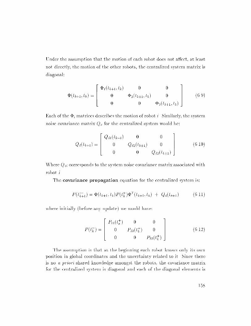
Under the assumption that the motion of each robot does not aect, at least
not directly, the motion of the other robots, the centralized system matrix is
diagonal:
(tk+1; tk) =
266641(tk+1; tk) 0 0
0 2(tk+1; tk) 0
0 0 3(tk+1; tk)
37775 (6.9)
Each of the i matrices describes the motion of robot i. Similarly, the system
noise covariance matrix Qd for the centralized system would be:
Qd(tk+1) =
26664Qd1(tk+1) 0 0
0 Qd2(tk+1) 0
0 0 Qd3(tk+1)
37775 (6.10)
Where Qdi corresponds to the system noise covariance matrix associated with
robot i.
The covariance propagation equation for the centralized system is:
P (tk+1) = (tk+1; tk)P (t+k )
T (tk+1; tk) + Qd(tk+1) (6.11)
where initially (before any update) we would have:
P (t+k ) =
26664P11(t
+k ) 0 0
0 P22(t+k ) 0
0 0 P33(t+k )
37775 (6.12)
The assumption is that at the beginning each robot knows only its own
position in global coordinates and the uncertainty related to it. Since there
is no a priori shared knowledge amongst the robots, the covariance matrix
for the centralized system is diagonal and each of the diagonal elements is
158
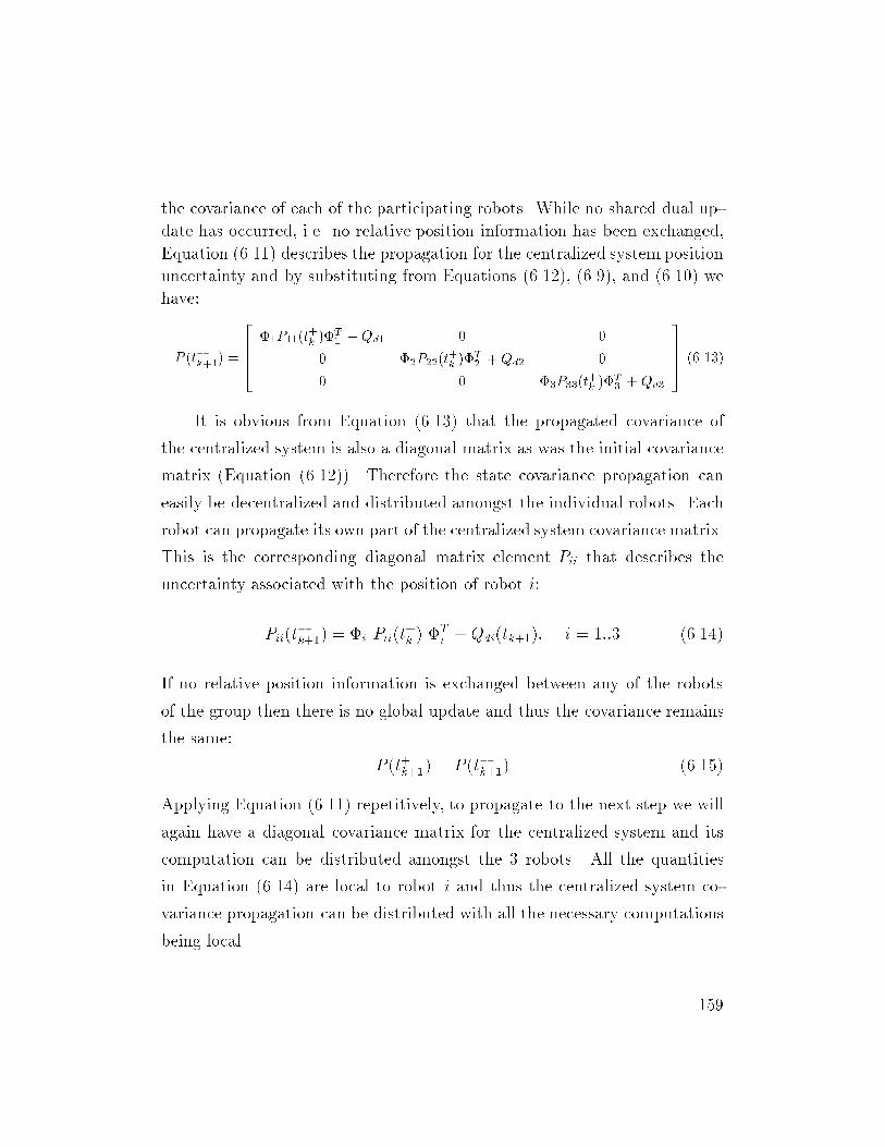
the covariance of each of the participating robots. While no shared dual up-
date has occurred, i.e. no relative position information has been exchanged,
Equation (6.11) describes the propagation for the centralized system position
uncertainty and by substituting from Equations (6.12), (6.9), and (6.10) we
have:
P (tk+1) =
2664
1P11(t+k )
T1 +Qd1 0 0
0 2P22(t+k )
T2 +Qd2 0
0 0 3P33(t+k )
T3 + Qd3
3775 (6.13)
It is obvious from Equation (6.13) that the propagated covariance of
the centralized system is also a diagonal matrix as was the initial covariance
matrix (Equation (6.12)). Therefore the state covariance propagation can
easily be decentralized and distributed amongst the individual robots. Each
robot can propagate its own part of the centralized system covariance matrix.
This is the corresponding diagonal matrix element Pii that describes the
uncertainty associated with the position of robot i:
Pii(tk+1) = i Pii(t
+k )
Ti +Qdi(tk+1); i = 1::3 (6.14)
If no relative position information is exchanged between any of the robots
of the group then there is no global update and thus the covariance remains
the same:
P (t+k+1) = P (tk+1) (6.15)
Applying Equation (6.11) repetitively, to propagate to the next step we will
again have a diagonal covariance matrix for the centralized system and its
computation can be distributed amongst the 3 robots. All the quantities
in Equation (6.14) are local to robot i and thus the centralized system co-
variance propagation can be distributed with all the necessary computations
being local.
159
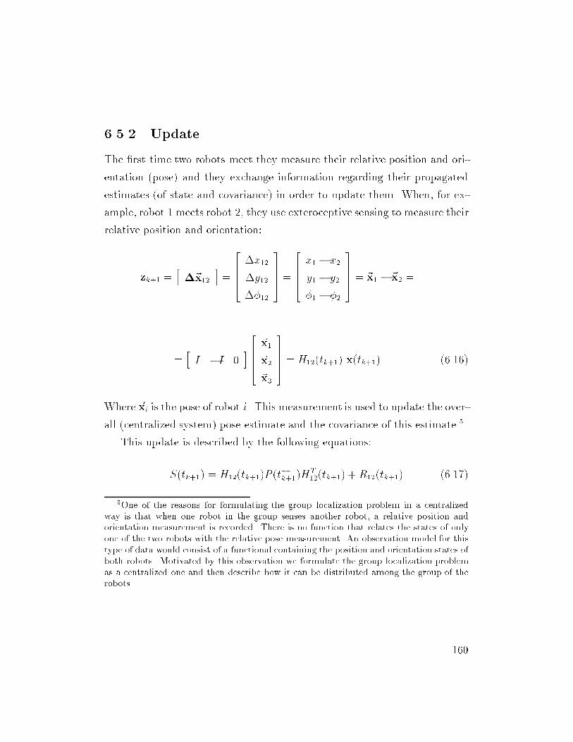
6.5.2 Update
The rst time two robots meet they measure their relative position and ori-
entation (pose) and they exchange information regarding their propagated
estimates (of state and covariance) in order to update them. When, for ex-
ample, robot 1 meets robot 2, they use exteroceptive sensing to measure their
relative position and orientation:
zk+1 =h~x12
i=
26664x12
y12
12
37775 =
26664x1 x2
y1 y2
1 2
37775 = ~x1 ~x2 =
=hI I 0
i26664~x1
~x2
~x3
37775 = H12(tk+1) x(tk+1) (6.16)
Where ~xi is the pose of robot i. This measurement is used to update the over-
all (centralized system) pose estimate and the covariance of this estimate.5
This update is described by the following equations:
S(tk+1) = H12(tk+1)P (tk+1)H
T12(tk+1) +R12(tk+1) (6.17)
5One of the reasons for formulating the group localization problem in a centralized
way is that when one robot in the group senses another robot, a relative position and
orientation measurement is recorded. There is no function that relates the states of only
one of the two robots with the relative pose measurement. An observation model for this
type of data would consist of a functional containing the position and orientation states of
both robots. Motivated by this observation we formulate the group localization problem
as a centralized one and then describe how it can be distributed among the group of the
robots.
160
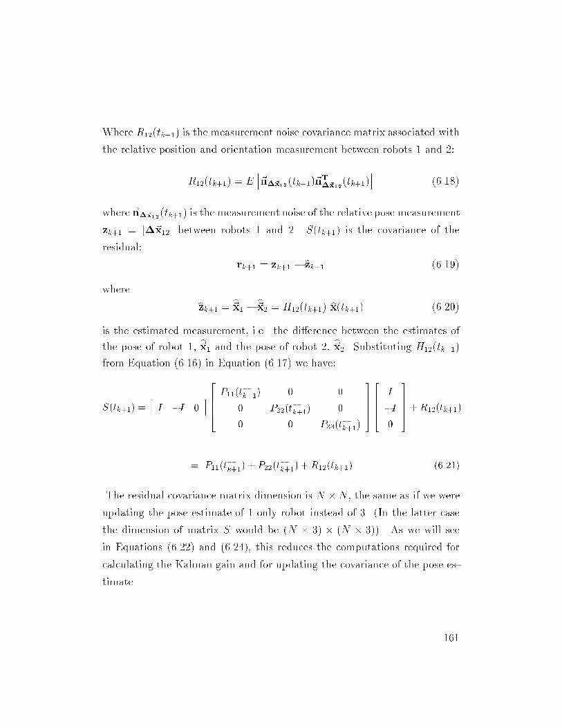
Where R12(tk+1) is the measurement noise covariance matrix associated with
the relative position and orientation measurement between robots 1 and 2:
R12(tk+1) = Eh~n~x12(tk+1)~n
T
~x12(tk+1)
i(6.18)
where ~n~x12(tk+1) is the measurement noise of the relative pose measurement
zk+1 = [~x12] between robots 1 and 2. S(tk+1) is the covariance of the
residual:
rk+1 = zk+1 bzk+1 (6.19)
where
bzk+1 = b~x1 b~x2 = H12(tk+1) bx(tk+1) (6.20)
is the estimated measurement, i.e. the dierence between the estimates of
the pose of robot 1, b~x1 and the pose of robot 2, b~x2. Substituting H12(tk+1)
from Equation (6.16) in Equation (6.17) we have:
S(tk+1) =hI I 0
i26664P11(t
k+1) 0 0
0 P22(tk+1) 0
0 0 P33(tk+1)
3777526664
I
I
0
37775+ R12(tk+1)
= P11(tk+1) + P22(t
k+1) + R12(tk+1) (6.21)
The residual covariance matrix dimension is N N , the same as if we were
updating the pose estimate of 1 only robot instead of 3. (In the latter case
the dimension of matrix S would be (N 3) (N 3)). As we will see
in Equations (6.22) and (6.24), this reduces the computations required for
calculating the Kalman gain and for updating the covariance of the pose es-
timate.
161
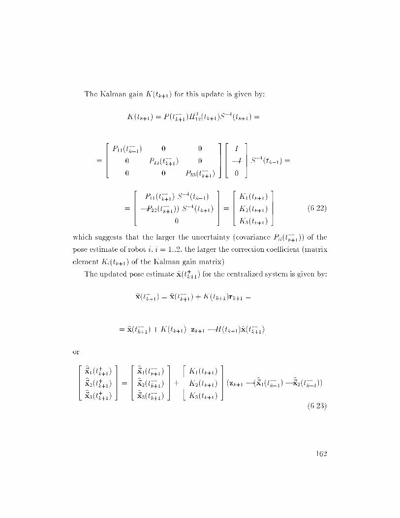
The Kalman gain K(tk+1) for this update is given by:
K(tk+1) = P (tk+1)HT12(tk+1)S
1(tk+1) =
=
26664P11(t
k+1) 0 0
0 P22(tk+1) 0
0 0 P33(tk+1)
3777526664
I
I
0
37775S1(tk+1) =
=
26664
P11(tk+1) S
1(tk+1)
P22(tk+1)) S
1(tk+1)
0
37775 =
26664K1(tk+1)
K2(tk+1)
K3(tk+1)
37775 (6.22)
which suggests that the larger the uncertainty (covariance Pii(tk+1)) of the
pose estimate of robot i, i = 1::2, the larger the correction coecient (matrix
element Ki(tk+1) of the Kalman gain matrix).
The updated pose estimate bx(t+k+1) for the centralized system is given by:
bx(t+k+1) = bx(tk+1) +K(tk+1)rk+1 =
= bx(tk+1) +K(tk+1)hzk+1 H(tk+1)bx(tk+1)i
or
26664b~x1(t+k+1)b~x2(t+k+1)b~x3(t+k+1)
37775 =
26664b~x1(tk+1)b~x2(tk+1)b~x3(tk+1)
37775+
26664K1(tk+1)
K2(tk+1)
K3(tk+1)
37775 (zk+1 (b~x1(tk+1) b~x2(tk+1))
(6.23)
162
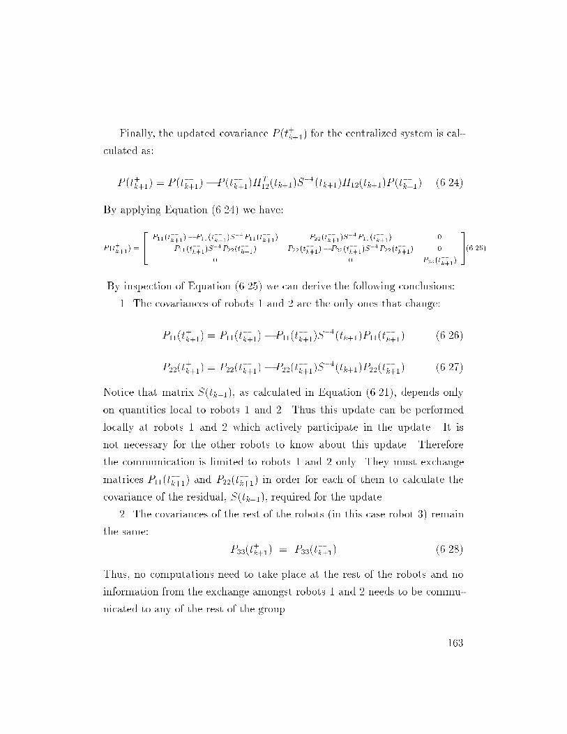
Finally, the updated covariance P (t+k+1) for the centralized system is cal-
culated as:
P (t+k+1) = P (tk+1) P (tk+1)HT12(tk+1)S
1(tk+1)H12(tk+1)P (tk+1) (6.24)
By applying Equation (6.24) we have:
P (t+k+1
) =
24 P11(t
k+1) P11(t
k+1)S1P11(t
k+1) P22(t
k+1)S1P11(t
k+1) 0
P11(t
k+1)S1P22(t
k+1) P22(t
k+1) P22(t
k+1)S1P22(t
k+1) 0
0 0 P33(t
k+1)
35(6.25)
By inspection of Equation (6.25) we can derive the following conclusions:
1. The covariances of robots 1 and 2 are the only ones that change:
P11(t+k+1) = P11(t
k+1) P11(t
k+1)S
1(tk+1)P11(tk+1) (6.26)
P22(t+k+1) = P22(t
k+1) P22(t
k+1)S
1(tk+1)P22(tk+1) (6.27)
Notice that matrix S(tk+1), as calculated in Equation (6.21), depends only
on quantities local to robots 1 and 2. Thus this update can be performed
locally at robots 1 and 2 which actively participate in the update. It is
not necessary for the other robots to know about this update. Therefore
the communication is limited to robots 1 and 2 only. They must exchange
matrices P11(tk+1) and P22(t
k+1) in order for each of them to calculate the
covariance of the residual, S(tk+1), required for the update.
2. The covariances of the rest of the robots (in this case robot 3) remain
the same:
P33(t+k+1) = P33(t
k+1) (6.28)
Thus, no computations need to take place at the rest of the robots and no
information from the exchange amongst robots 1 and 2 needs to be commu-
nicated to any of the rest of the group.
163
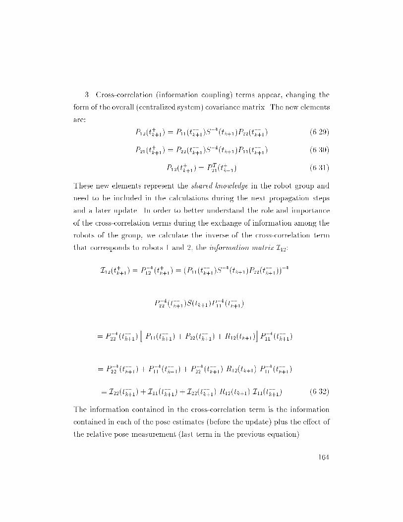
3. Cross-correlation (information coupling) terms appear, changing the
form of the overall (centralized system) covariance matrix. The new elements
are:
P12(t+k+1) = P11(t
k+1)S
1(tk+1)P22(tk+1) (6.29)
P21(t+k+1) = P22(t
k+1)S
1(tk+1)P11(tk+1) (6.30)
P12(t+k+1) = P T
21(t+k+1) (6.31)
These new elements represent the shared knowledge in the robot group and
need to be included in the calculations during the next propagation steps
and a later update. In order to better understand the role and importance
of the cross-correlation terms during the exchange of information among the
robots of the group, we calculate the inverse of the cross-correlation term
that corresponds to robots 1 and 2, the information matrix I12:
I12(t+k+1) = P112 (t+k+1) = (P11(t
k+1)S
1(tk+1)P22(tk+1))
1
= P122 (tk+1)S(tk+1)P
111 (t
k+1)
= P122 (tk+1)
hP11(t
k+1) + P22(t
k+1) +R12(tk+1)
iP111 (t
k+1)
= P122 (tk+1) + P111 (t
k+1) + P122 (t
k+1) R12(tk+1) P
111 (t
k+1)
= I22(tk+1) + I11(tk+1) + I22(t
k+1) R12(tk+1) I11(tk+1) (6.32)
The information contained in the cross-correlation term is the information
contained in each of the pose estimates (before the update) plus the eect of
the relative pose measurement (last term in the previous equation).
164
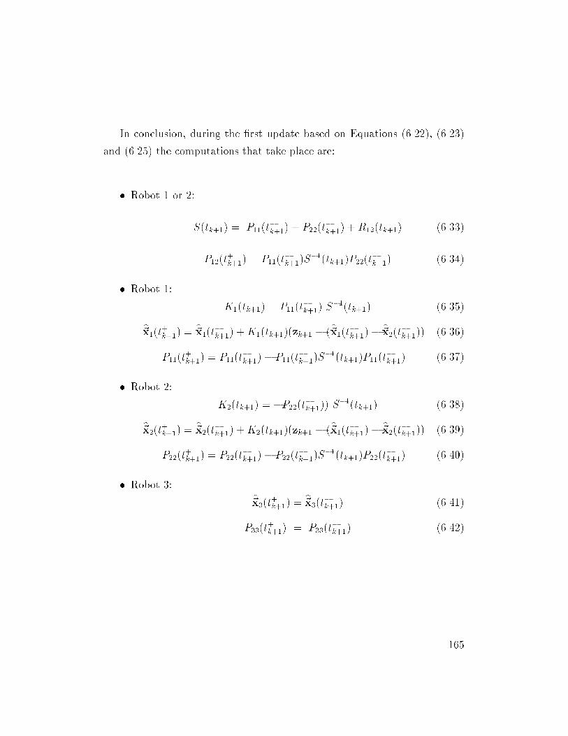
In conclusion, during the rst update based on Equations (6.22), (6.23)
and (6.25) the computations that take place are:
Robot 1 or 2:
S(tk+1) = P11(tk+1) + P22(t
k+1) +R12(tk+1) (6.33)
P12(t+k+1) = P11(t
k+1)S
1(tk+1)P22(tk+1) (6.34)
Robot 1:
K1(tk+1) = P11(tk+1) S
1(tk+1) (6.35)
b~x1(t+k+1) = b~x1(tk+1) +K1(tk+1)(zk+1 (b~x1(tk+1) b~x2(tk+1)) (6.36)
P11(t+k+1) = P11(t
k+1) P11(t
k+1)S
1(tk+1)P11(tk+1) (6.37)
Robot 2:
K2(tk+1) = P22(tk+1)) S
1(tk+1) (6.38)
b~x2(t+k+1) = b~x2(tk+1) +K2(tk+1)(zk+1 (b~x1(tk+1) b~x2(tk+1)) (6.39)
P22(t+k+1) = P22(t
k+1) P22(t
k+1)S
1(tk+1)P22(tk+1) (6.40)
Robot 3: b~x3(t+k+1) = b~x3(tk+1) (6.41)
P33(t+k+1) = P33(t
k+1) (6.42)
165
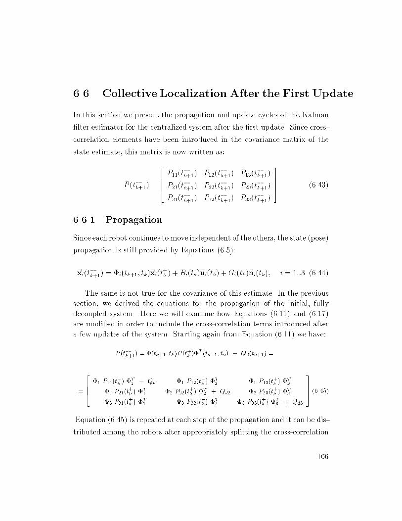
6.6 Collective Localization After the First Update
In this section we present the propagation and update cycles of the Kalman
lter estimator for the centralized system after the rst update. Since cross-
correlation elements have been introduced in the covariance matrix of the
state estimate, this matrix is now written as:
P (tk+1) =
26664P11(t
k+1) P12(t
k+1) P13(t
k+1)
P21(tk+1) P22(t
k+1) P23(t
k+1)
P31(tk+1) P32(t
k+1) P33(t
k+1)
37775 (6.43)
6.6.1 Propagation
Since each robot continues to move independent of the others, the state (pose)
propagation is still provided by Equations (6.5):
~xi(tk+1) = i(tk+1; tk)~xi(t
+k ) +Bi(tk)~ui(tk) +Gi(tk)~ni(tk); i = 1::3 (6.44)
The same is not true for the covariance of this estimate. In the previous
section, we derived the equations for the propagation of the initial, fully
decoupled system. Here we will examine how Equations (6.11) and (6.17)
are modied in order to include the cross-correlation terms introduced after
a few updates of the system. Starting again from Equation (6.11) we have:
P (tk+1) = (tk+1; tk)P (t+k )
T (tk+1; tk) + Qd(tk+1) =
=
2664
1 P11(t+k )
T1 + Qd1 1 P12(t
+k )
T2 1 P13(t
+k )
T3
2 P21(t+k )
T1 2 P22(t
+k )
T2 + Qd2 2 P23(t
+k )
T3
3 P31(t+k )
T1 3 P32(t
+k )
T2 3 P33(t
+k )
T3 + Qd3
3775 (6.45)
Equation (6.45) is repeated at each step of the propagation and it can be dis-
tributed among the robots after appropriately splitting the cross-correlation
166
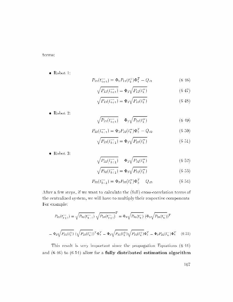
terms:
Robot 1:
P11(tk+1) = 1P11(t
+k )
T1 +Qd1 (6.46)q
P12(tk+1) = 1
qP12(t
+k ) (6.47)q
P13(tk+1) = 1
qP13(t
+k ) (6.48)
Robot 2: qP21(t
k+1) = 2
qP21(t
+k ) (6.49)
P22(tk+1) = 2P22(t
+k )
T2 +Qd2 (6.50)q
P23(tk+1) = 2
qP23(t
+k ) (6.51)
Robot 3: qP31(t
k+1) = 3
qP31(t
+k ) (6.52)q
P32(tk+1) = 3
qP32(t
+k ) (6.53)
P33(tk+1) = 3P33(t
+k )
T3 +Qd3 (6.54)
After a few steps, if we want to calculate the (full) cross-correlation terms of
the centralized system, we will have to multiply their respective components.
For example:
P32(t
k+1) =
qP32(t
k+1)
qP23(t
k+1)T
= 3
qP32(t
+k ) (2
qP23(t
+k ))
T
= 3
qP32(t
+k ) (
qP23(t
+k ))
TT2 = 3
qP32(t
+k )
qP32(t
+k )
T2 = 3P32(t
+k )
T2 (6.55)
This result is very important since the propagation Equations (6.44)
and (6.46) to (6.54) allow for a fully distributed estimation algorithm
167
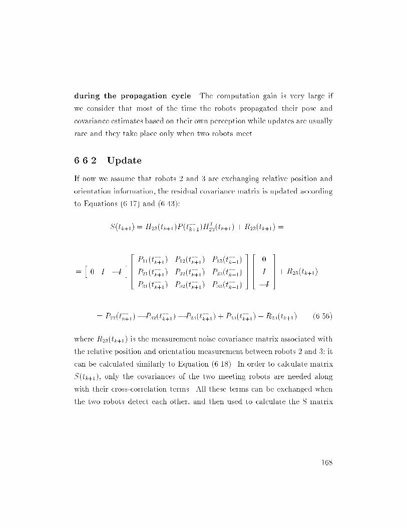
during the propagation cycle. The computation gain is very large if
we consider that most of the time the robots propagated their pose and
covariance estimates based on their own perception while updates are usually
rare and they take place only when two robots meet.
6.6.2 Update
If now we assume that robots 2 and 3 are exchanging relative position and
orientation information, the residual covariance matrix is updated according
to Equations (6.17) and (6.43):
S(tk+1) = H23(tk+1)P (tk+1)H
T23(tk+1) +R23(tk+1) =
=h0 I I
i26664P11(t
k+1) P12(t
k+1) P13(t
k+1)
P21(tk+1) P22(t
k+1) P23(t
k+1)
P31(tk+1) P32(t
k+1) P33(t
k+1)
3777526664
0
I
I
37775+R23(tk+1)
= P22(tk+1) P32(t
k+1) P23(t
k+1) + P33(t
k+1) +R23(tk+1) (6.56)
where R23(tk+1) is the measurement noise covariance matrix associated with
the relative position and orientation measurement between robots 2 and 3; it
can be calculated similarly to Equation (6.18). In order to calculate matrix
S(tk+1), only the covariances of the two meeting robots are needed along
with their cross-correlation terms. All these terms can be exchanged when
the two robots detect each other, and then used to calculate the S matrix
168
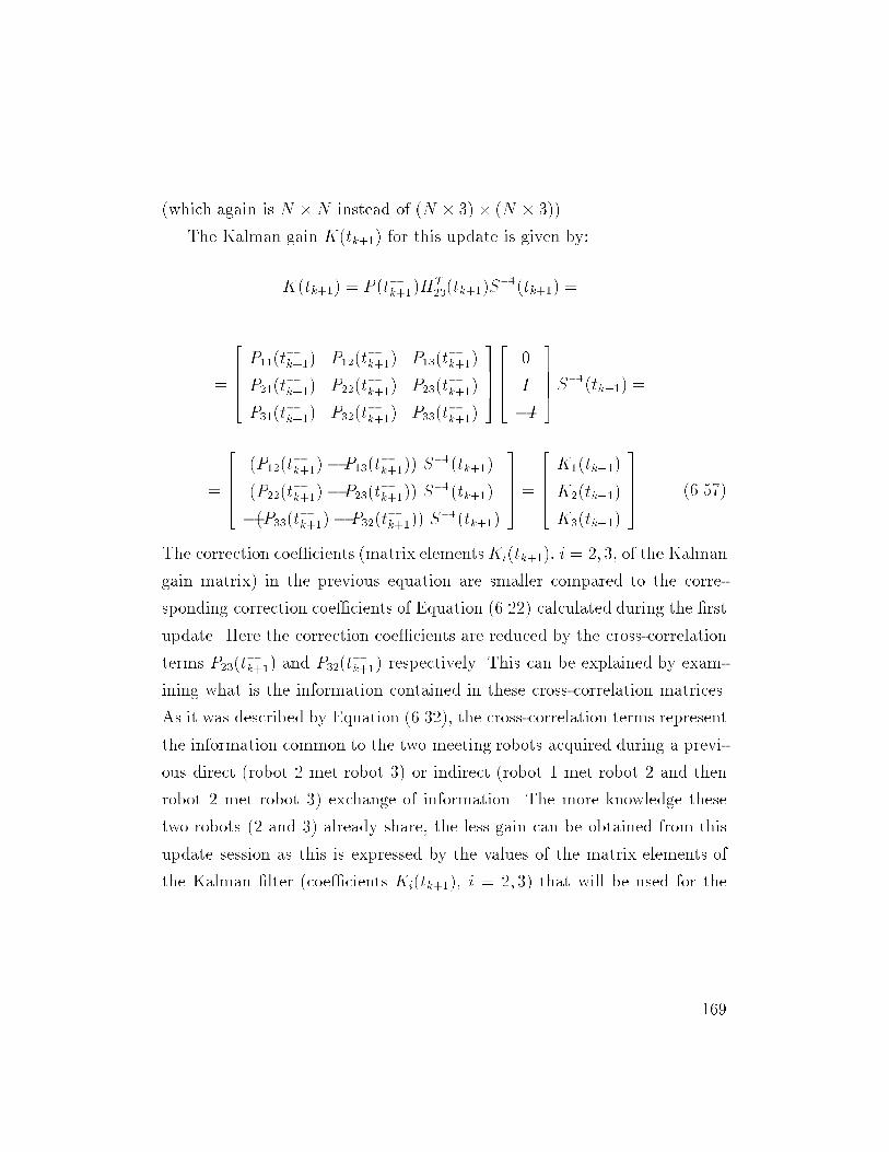
(which again is N N instead of (N 3) (N 3)).
The Kalman gain K(tk+1) for this update is given by:
K(tk+1) = P (tk+1)HT23(tk+1)S
1(tk+1) =
=
26664P11(t
k+1) P12(t
k+1) P13(t
k+1)
P21(tk+1) P22(t
k+1) P23(t
k+1)
P31(tk+1) P32(t
k+1) P33(t
k+1)
3777526664
0
I
I
37775S1(tk+1) =
=
26664
(P12(tk+1) P13(t
k+1)) S
1(tk+1)
(P22(tk+1) P23(t
k+1)) S
1(tk+1)
(P33(tk+1) P32(t
k+1)) S
1(tk+1)
37775 =
26664K1(tk+1)
K2(tk+1)
K3(tk+1)
37775 (6.57)
The correction coecients (matrix elementsKi(tk+1), i = 2; 3, of the Kalman
gain matrix) in the previous equation are smaller compared to the corre-
sponding correction coecients of Equation (6.22) calculated during the rst
update. Here the correction coecients are reduced by the cross-correlation
terms P23(tk+1) and P32(t
k+1) respectively. This can be explained by exam-
ining what is the information contained in these cross-correlation matrices.
As it was described by Equation (6.32), the cross-correlation terms represent
the information common to the two meeting robots acquired during a previ-
ous direct (robot 2 met robot 3) or indirect (robot 1 met robot 2 and then
robot 2 met robot 3) exchange of information. The more knowledge these
two robots (2 and 3) already share, the less gain can be obtained from this
update session as this is expressed by the values of the matrix elements of
the Kalman lter (coecients Ki(tk+1), i = 2; 3) that will be used for the
169
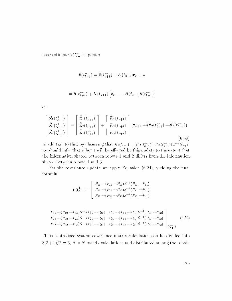
pose estimate bx(t+k+1) update:
bx(t+k+1) = bx(tk+1) +K(tk+1)rk+1 =
= bx(tk+1) +K(tk+1)hzk+1 H(tk+1)bx(tk+1)i
or
26664b~x1(t+k+1)b~x2(t+k+1)b~x3(t+k+1)
37775 =
26664b~x1(tk+1)b~x2(tk+1)b~x3(tk+1)
37775+
26664K1(tk+1)
K2(tk+1)
K3(tk+1)
37775 (zk+1 (b~x2(tk+1) b~x3(tk+1))
(6.58)
In addition to this, by observing that K1(tk+1) = (P12(t
k+1)P13(t
k+1)) S1(tk+1)
we should infer that robot 1 will be aected by this update to the extent that
the information shared between robots 1 and 2 diers from the information
shared between robots 1 and 3.
For the covariance update we apply Equation (6.24), yielding the nal
formula:
P (t+k+1) =
2664
P11 (P12 P13)S1(P21 P31)
P21 (P22 P23)S1(P21 P31)
P31 (P32 P33)S1(P21 P31)
P12 (P12 P13)S1(P22 P32) P13 (P12 P13)S
1(P23 P33)
P22 (P22 P23)S1(P22 P32) P23 (P22 P23)S
1(P23 P33)
P32 (P32 P33)S1(P22 P32) P33 (P32 P33)S
1(P23 P33)
3775(t
k+1)
(6.59)
This centralized system covariance matrix calculation can be divided into
3(3+1)=2 = 6, N N matrix calculations and distributed among the robots
170
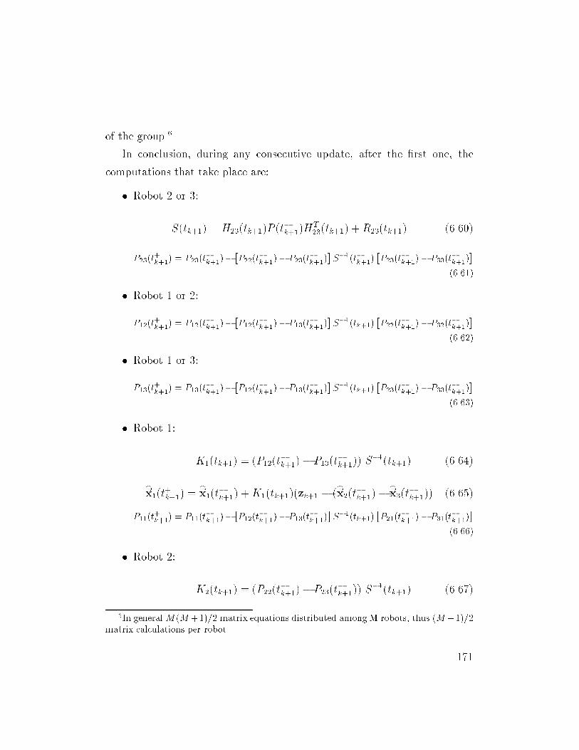
of the group.6
In conclusion, during any consecutive update, after the rst one, the
computations that take place are:
Robot 2 or 3:
S(tk+1) = H23(tk+1)P (tk+1)H
T23(tk+1) +R23(tk+1) (6.60)
P23(t+k+1) = P23(t
k+1)P22(t
k+1) P23(t
k+1)S1(tk+1)
P23(t
k+1) P33(t
k+1)
(6.61)
Robot 1 or 2:
P12(t+k+1) = P12(t
k+1)P12(t
k+1) P13(t
k+1)S1(tk+1)
P22(t
k+1) P32(t
k+1)
(6.62)
Robot 1 or 3:
P13(t+k+1) = P13(t
k+1)P12(t
k+1) P13(t
k+1)S1(tk+1)
P23(t
k+1) P33(t
k+1)
(6.63)
Robot 1:
K1(tk+1) = (P12(tk+1) P13(t
k+1)) S
1(tk+1) (6.64)
b~x1(t+k+1) = b~x1(tk+1) +K1(tk+1)(zk+1 (b~x2(tk+1) b~x3(tk+1)) (6.65)
P11(t+k+1) = P11(t
k+1)P12(t
k+1) P13(t
k+1)S1(tk+1)
P21(t
k+1) P31(t
k+1)
(6.66)
Robot 2:
K2(tk+1) = (P22(tk+1) P23(t
k+1)) S
1(tk+1) (6.67)
6In general M (M +1)=2 matrix equations distributed among M robots, thus (M+1)=2matrix calculations per robot.
171
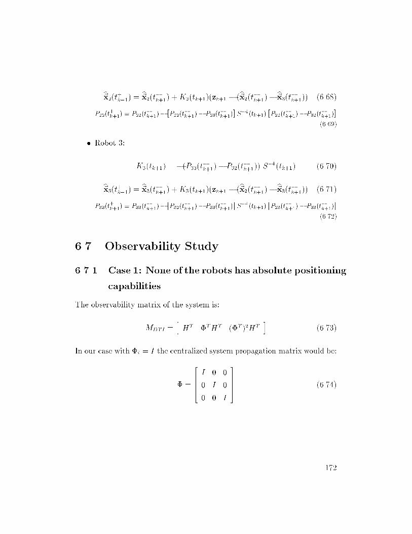
b~x2(t+k+1) = b~x2(tk+1) +K2(tk+1)(zk+1 (b~x2(tk+1) b~x3(tk+1)) (6.68)
P22(t+k+1) = P22(t
k+1)P22(t
k+1) P23(t
k+1)S1(tk+1)
P22(t
k+1) P32(t
k+1)
(6.69)
Robot 3:
K3(tk+1) = (P33(tk+1) P32(t
k+1)) S
1(tk+1) (6.70)
b~x3(t+k+1) = b~x3(tk+1) +K3(tk+1)(zk+1 (b~x2(tk+1) b~x3(tk+1)) (6.71)
P33(t+k+1) = P33(t
k+1)P32(t
k+1) P33(t
k+1)S1(tk+1)
P23(t
k+1) P33(t
k+1)
(6.72)
6.7 Observability Study
6.7.1 Case 1: None of the robots has absolute positioning
capabilities
The observability matrix of the system is:
MDTI =hHT THT (T )2HT
i(6.73)
In our case with i = I the centralized system propagation matrix would be:
=
26664I 0 0
0 I 0
0 0 I
37775 (6.74)
172
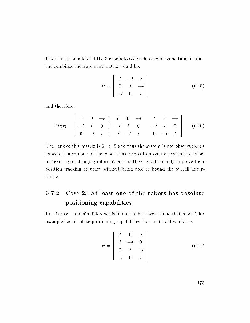
If we choose to allow all the 3 robots to see each other at some time instant,
the combined measurement matrix would be:
H =
26664
I I 0
0 I I
I 0 I
37775 (6.75)
and therefore:
MDTI =
26664
I 0 I j I 0 I j I 0 I
I I 0 j I I 0 j I I 0
0 I I j 0 I I j 0 I I
37775 (6.76)
The rank of this matrix is 6 < 9 and thus the system is not observable, as
expected since none of the robots has access to absolute positioning infor-
mation. By exchanging information, the three robots merely improve their
position tracking accuracy without being able to bound the overall uncer-
tainty.
6.7.2 Case 2: At least one of the robots has absolute
positioning capabilities
In this case the main dierence is in matrix H. If we assume that robot 1 for
example has absolute positioning capabilities then matrix H would be:
H =
26666664
I 0 0
I I 0
0 I I
I 0 I
37777775 (6.77)
173
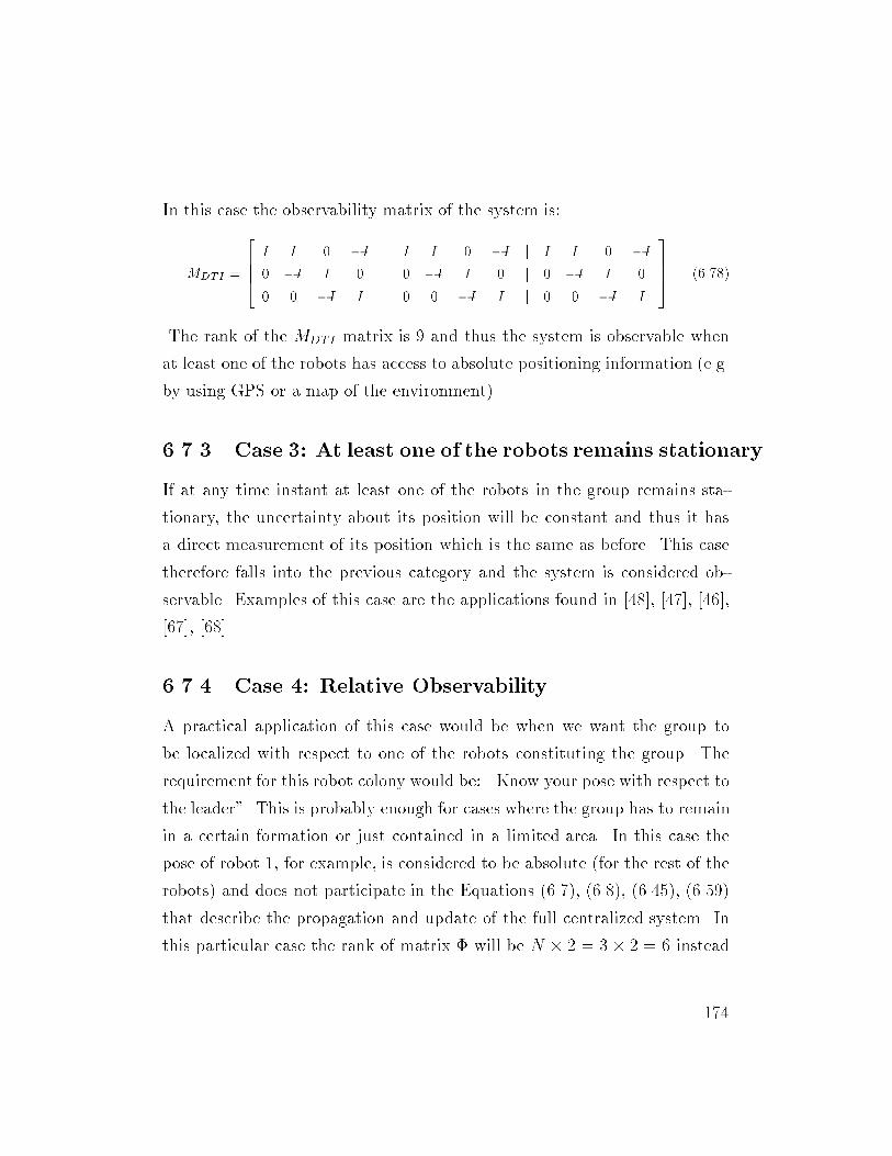
In this case the observability matrix of the system is:
MDTI =
2664
I I 0 I j I I 0 I j I I 0 I
0 I I 0 j 0 I I 0 j 0 I I 0
0 0 I I j 0 0 I I j 0 0 I I
3775 (6.78)
The rank of the MDTI matrix is 9 and thus the system is observable when
at least one of the robots has access to absolute positioning information (e.g.
by using GPS or a map of the environment).
6.7.3 Case 3: At least one of the robots remains stationary
If at any time instant at least one of the robots in the group remains sta-
tionary, the uncertainty about its position will be constant and thus it has
a direct measurement of its position which is the same as before. This case
therefore falls into the previous category and the system is considered ob-
servable. Examples of this case are the applications found in [48], [47], [46],
[67], [68].
6.7.4 Case 4: Relative Observability
A practical application of this case would be when we want the group to
be localized with respect to one of the robots constituting the group. The
requirement for this robot colony would be: \Know your pose with respect to
the leader". This is probably enough for cases where the group has to remain
in a certain formation or just contained in a limited area. In this case the
pose of robot 1, for example, is considered to be absolute (for the rest of the
robots) and does not participate in the Equations (6.7), (6.8), (6.45), (6.59)
that describe the propagation and update of the full centralized system. In
this particular case the rank of matrix will be N 2 = 3 2 = 6 instead
174
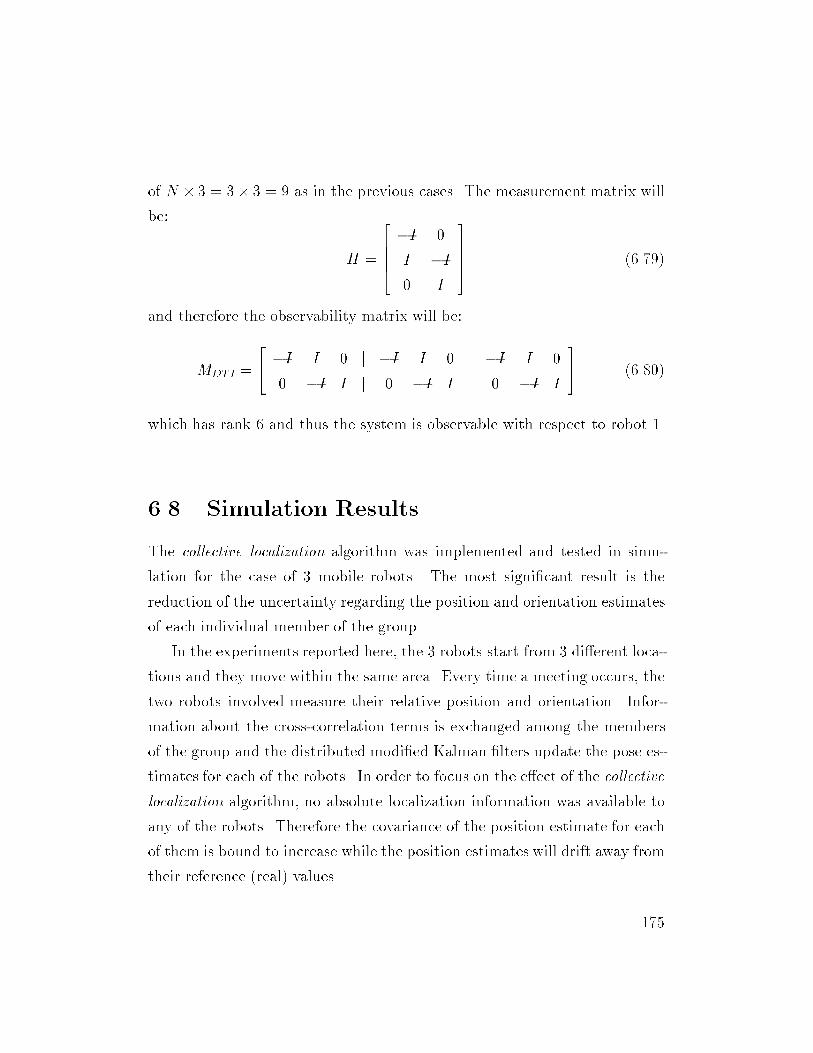
of N 3 = 3 3 = 9 as in the previous cases. The measurement matrix will
be:
H =
26664I 0
I I
0 I
37775 (6.79)
and therefore the observability matrix will be:
MDTI =
24 I I 0 j I I 0 j I I 0
0 I I j 0 I I j 0 I I
35 (6.80)
which has rank 6 and thus the system is observable with respect to robot 1.
6.8 Simulation Results
The collective localization algorithm was implemented and tested in simu-
lation for the case of 3 mobile robots. The most signicant result is the
reduction of the uncertainty regarding the position and orientation estimates
of each individual member of the group.
In the experiments reported here, the 3 robots start from 3 dierent loca-
tions and they move within the same area. Every time a meeting occurs, the
two robots involved measure their relative position and orientation. Infor-
mation about the cross-correlation terms is exchanged among the members
of the group and the distributed modied Kalman lters update the pose es-
timates for each of the robots. In order to focus on the eect of the collective
localization algorithm, no absolute localization information was available to
any of the robots. Therefore the covariance of the position estimate for each
of them is bound to increase while the position estimates will drift away from
their reference (real) values.
175
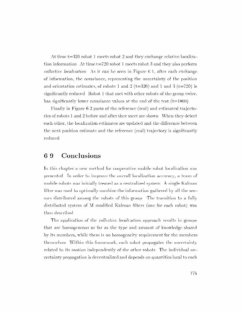
At time t=320 robot 1 meets robot 2 and they exchange relative localiza-
tion information. At time t=720 robot 1 meets robot 3 and they also perform
collective localization. As it can be seen in Figure 6.1, after each exchange
of information, the covariance, representing the uncertainty of the position
and orientation estimates, of robots 1 and 2 (t=320) and 1 and 3 (t=720) is
signicantly reduced. Robot 1 that met with other robots of the group twice,
has signicantly lower covariance values at the end of the test (t=1000).
Finally in Figure 6.2 parts of the reference (real) and estimated trajecto-
ries of robots 1 and 2 before and after they meet are shown. When they detect
each other, the localization estimates are updated and the dierence between
the next position estimate and the reference (real) trajectory is signicantly
reduced.
6.9 Conclusions
In this chapter a new method for cooperative mobile robot localization was
presented. In order to improve the overall localization accuracy, a team of
mobile robots was initially treated as a centralized system. A single Kalman
lter was used to optimally combine the information gathered by all the sen-
sors distributed among the robots of this group. The transition to a fully
distributed system of M modied Kalman lters (one for each robot) was
then described.
The application of the collective localization approach results in groups
that are homogeneous as far as the type and amount of knowledge shared
by its members, while there is no homogeneity requirement for the members
themselves. Within this framework, each robot propagates the uncertainty
related to its motion independently of the other robots. The individual un-
certainty propagation is decentralized and depends on quantities local to each
176
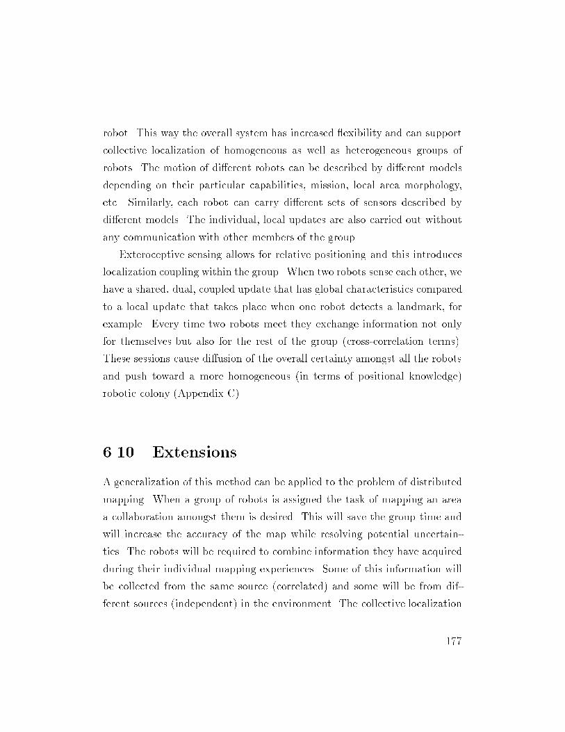
robot. This way the overall system has increased exibility and can support
collective localization of homogeneous as well as heterogeneous groups of
robots. The motion of dierent robots can be described by dierent models
depending on their particular capabilities, mission, local area morphology,
etc. Similarly, each robot can carry dierent sets of sensors described by
dierent models. The individual, local updates are also carried out without
any communication with other members of the group.
Exteroceptive sensing allows for relative positioning and this introduces
localization coupling within the group. When two robots sense each other, we
have a shared, dual, coupled update that has global characteristics compared
to a local update that takes place when one robot detects a landmark, for
example. Every time two robots meet they exchange information not only
for themselves but also for the rest of the group (cross-correlation terms).
These sessions cause diusion of the overall certainty amongst all the robots
and push toward a more homogeneous (in terms of positional knowledge)
robotic colony (Appendix C).
6.10 Extensions
A generalization of this method can be applied to the problem of distributed
mapping. When a group of robots is assigned the task of mapping an area
a collaboration amongst them is desired. This will save the group time and
will increase the accuracy of the map while resolving potential uncertain-
ties. The robots will be required to combine information they have acquired
during their individual mapping experiences. Some of this information will
be collected from the same source (correlated) and some will be from dif-
ferent sources (independent) in the environment. The collective localization
177

methodology can potentially be extended to describe the fusion of informa-
tion collected by the dierent members of the group in order to produce a
combined and uniform map of the area.
178
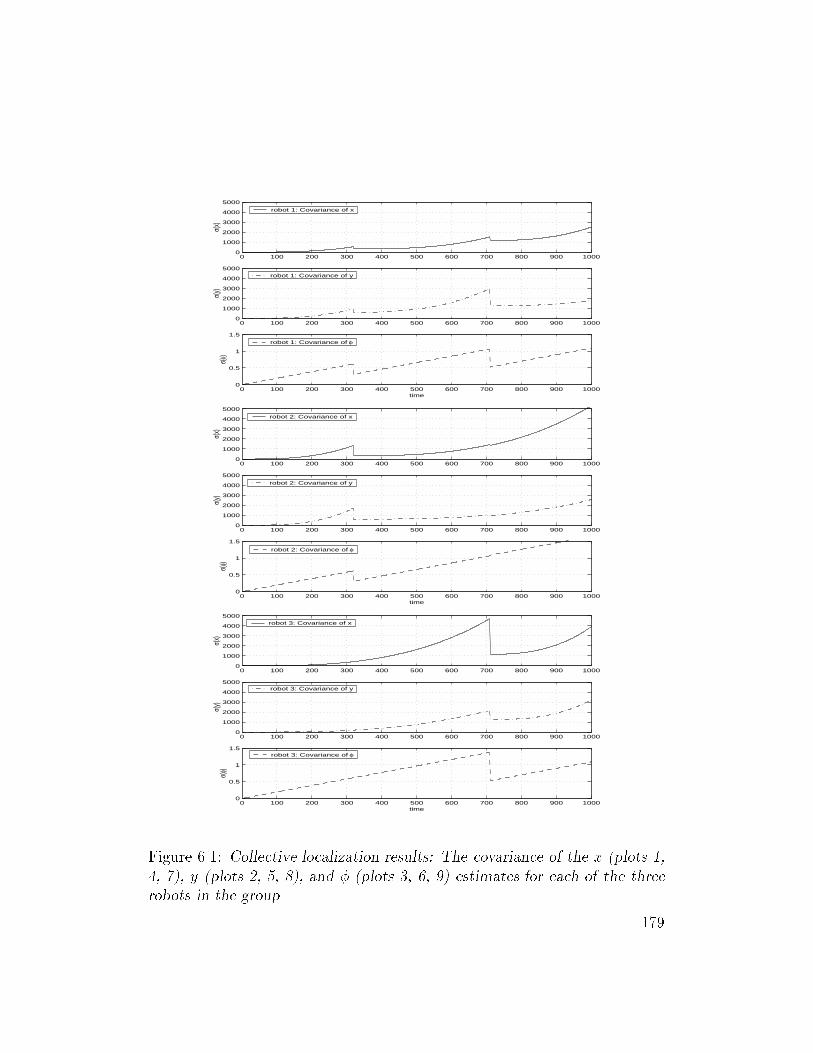
0 100 200 300 400 500 600 700 800 900 10000
1000
2000
3000
4000
5000
σ(x)
robot 1: Covariance of x
0 100 200 300 400 500 600 700 800 900 10000
1000
2000
3000
4000
5000
σ(y)
robot 1: Covariance of y
0 100 200 300 400 500 600 700 800 900 10000
0.5
1
1.5
σ(φ)
time
robot 1: Covariance of φ
0 100 200 300 400 500 600 700 800 900 10000
1000
2000
3000
4000
5000
σ(x)
robot 2: Covariance of x
0 100 200 300 400 500 600 700 800 900 10000
1000
2000
3000
4000
5000
σ(y)
robot 2: Covariance of y
0 100 200 300 400 500 600 700 800 900 10000
0.5
1
1.5
σ(φ)
time
robot 2: Covariance of φ
0 100 200 300 400 500 600 700 800 900 10000
1000
2000
3000
4000
5000
σ(x)
robot 3: Covariance of x
0 100 200 300 400 500 600 700 800 900 10000
1000
2000
3000
4000
5000
σ(y)
robot 3: Covariance of y
0 100 200 300 400 500 600 700 800 900 10000
0.5
1
1.5
σ(φ)
time
robot 3: Covariance of φ
Figure 6.1: Collective localization results: The covariance of the x (plots 1,
4, 7), y (plots 2, 5, 8), and (plots 3, 6, 9) estimates for each of the three
robots in the group.
179
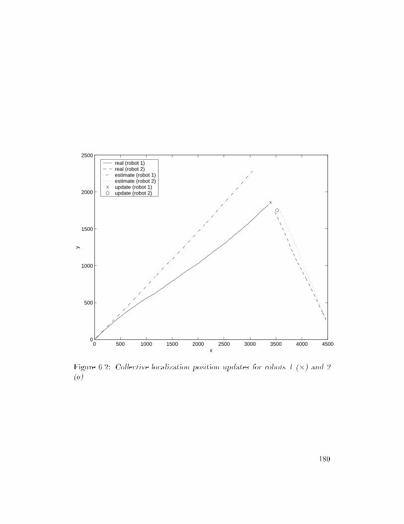
0 500 1000 1500 2000 2500 3000 3500 4000 45000
500
1000
1500
2000
2500
y
x
real (robot 1) real (robot 2) estimate (robot 1)estimate (robot 2)update (robot 1) update (robot 2)
Figure 6.2: Collective localization position updates for robots 1 () and 2
(o).
180
Chapter 7
Reference List
[1] R. O. Allen and D. H. Chang. Performance testing of the Systron Donner
quartz gyro. JPL Engineering Memorandum, EM #343-1297, January
5, 1993.
[2] D. Avis and H. Imai. Locating a robot with angle measurements. Jour-
nal of Symbolic Computation, 10(3-4):311326, Sept.-Oct. 1990.
[3] Y. Bar-Shalom and T. E. Fortmann. Tracking and Data Association.
Academic Press, New York, 1988.
[4] B. Barshan and H. F. Durrant-Whyte. Inertial navigation systems
for mobile robots. IEEE Transactions on Robotics and Automation,
11(3):328342, June 1995.
[5] E. T. Baumgartner and S. B. Skaar. An autonomous vision-based mobile
robot. IEEE Transactions on Automatic Control, 39(3):493501, March
1994.
[6] M. Betke and L. Gurvits. Mobile robot localization using landmarks.
IEEE Transactions on Robotics and Automation, 13(2):251263, April
1997.
[7] Ph. Bonnifait and G. Garcia. A multisensor localization algorithm for
mobile robots and it's real-time experimental validation. In Proceedings
of the 1996 IEEE International Conference on Robotics and Automation,
pages 13951400, 1996.
181
[8] J. Borenstein. Control and kinematic design of multi-degree-of freedom
mobile robots with compliant linkage. IEEE Transactions on Robotics
and Automation, 11(1):2135, Feb. 1995.
[9] J. Borenstein. Internal correction of dead-reckoning errors with a dual-
drive compliant linkage mobile robot. Journal of Robotic Systems,
12(4):257273, April 1995.
[10] J. Borenstein. Experimental results from internal odometry error correc-
tion with the omnimate mobile robot. IEEE Transactions on Robotics
and Automation, 14(6):963969, Dec. 1998.
[11] J. Borenstein and L. Feng. Correction of systematic odometry errors in
mobile robots. In Proceedings of the 1995 IEEE International Confer-
ence on Robotics and Automation, pages 569574, 1995.
[12] J. Borenstein and L. Feng. Gyrodometry: A new method for combining
data from gyros and odometry in mobile robots. In Proceedings of the
1996 IEEE International Conference on Robotics and Automation, pages
423428, 1996.
[13] J. C. K. Chou. Quaternion kinematic and dynamic dierential equa-
tions. IEEE Transactions on Robotics and Automation, 8(1):5364, Feb.
1992.
[14] M. Collett, T. S. Collett, S. Bisch, and R. Wehner. Local and global
vectors in desert ant navigation. Nature, 394(6690):269272, 1998.
[15] S. Cooper and H. F. Durrant-Whyte. A frequency response method for
multi-sensor high-speed navigation systems. In Proceedings of the 1994
IEEE International Conference on Multisensor Fusion and Integration
Systems, pages 18, Las Vegas, NV, 2-5 Oct. 1994.
[16] I. J. Cox and J. J. Leonard. Modeling a dynamic environment us-
ing a Bayesian multiple hypothesis approach. Articial Intelligence,
66(2):311344, April 1994.
182
[17] F. Cozman and E. Krotkov. Robot localization using a computer vi-
sion sextant. In Proceedings of the IEEE International Conference on
Robotics and Automation, pages 106111, Nagoya, Japan, 21-27 May
1995.
[18] F. Cozman and E. Krotkov. Automatic mountain detection and pose
estimation for teleoperation of lunar rovers. In Proceedings of the 1997
IEEE International Conference on Robotics and Automation, volume 3,
pages 24522457, New York, NY, April 1997.
[19] J. J. Craig. Introduction to Robotics, chapter 2, pages 5556. Addison-
Wesley, 2nd edition, 1989.
[20] T. Denmeade. A pioneer's journey into the sarcophagus. Nuclear Engi-
neering International, 43(524):1820, March 1998.
[21] H. F. Durrant-Whyte. Where am I? A tutorial on mobile vehicle local-
ization. Industrial Robot, 21(2):1116, 1994.
[22] A. Dushman. On gyro drift models and their evaluation. IRE Transac-
tions on Aerospace and Navigational Electronics, ANE-9:230234, Dec.
1962.
[23] A. Elfes. Using occupancy grids for mobile robot perception and navi-
gation. Computer, 22(6):4657, June 1989.
[24] R. Epstein and N. Kanwisher. A cortical representation of the local
visual environment. Nature, 392(6676):598601, 1998.
[25] R. L. Farrenkopf. Analytic steady-state accuracy solutions for two com-
mon spacecraft estimators. Journal of Guidance and Control, 1:282284,
July-Aug. 1978.
[26] A.M. Flynn. Combining sonar and infrared sensors for mobile robot
navigation. International Journal of Robotics Research, 7(6):514, Dec.
1988.
[27] M.S. Fontan and M.J. Mataric. Territorial multi-robot task division.
IEEE Transactions on Robotics and Automation, 14(5):815822, Oct.
1998.
183
[28] Y. Fuke and E. Krotkov. Dead reckoning for a lunar rover on uneven
terrain. In Proceedings of the 1996 IEEE International Conference on
Robotics and Automation, pages 411416, 1996.
[29] A. Gelb, editor. Applied Optimal Estimation, chapter 5. M.I.T. Press,
1994.
[30] C. R. Giardina, R. Bronson, and L. Wallen. An optimal normalization
scheme. IEEE Transactions on Aerospace and Electronic Systems, AES-
11:443446, July 1975.
[31] C. H. Greene and R. G. Cook. Landmark geometry and identity controls
spatial navigation in rats. Animal Learning & Behavior, 25(3):312323,
1997.
[32] M. S. Grewal and A. P. Andrews. Kalman Filtering, Theory and Prac-
tice. Prentice Hall, 1993.
[33] W. E. L. Grimson and T. Lozano-Perez. Localizing overlapping parts
by searching the interpretation tree. IEEE Transactions on Pattern
Analysis and Machine Intelligence, PAMI-9(4):469482, July 1987.
[34] J.-S. Gutmann, W. Burgard, D. Fox, and K. Konolige. An experi-
mental comparison of localization methods. In Proceedings of the 1998
IEEE/RSJ International Conference on Intelligent Robots and Systems,
pages 736743, Victoria, BC, Canada, Oct. 13-17 1998.
[35] N. Hager, A. Cypher, and D. C. Smith. Cocoa at the visual program-
ming challenge 1997. Computing, 9(2):151169, April 1998.
[36] W. R. Hamilton. Elements of Quaternions. Longmans, Green and Co.,
London, 1866.
[37] R. L. Hammon. An application of random process theory to gyro drift
analysis. IRE Transactions on Aeronautical and Navigational Electron-
ics, ANE-7:230234, Dec. 1962.
[38] U. D. Hanebeck and G. Schmidt. Set theoretic localization of fast mo-
bile robots using an angle measurement. In Proceedings of the 1996 In-
ternational Conference on Robotics and Automation, pages 13871394,
Minneapolis, MN, April 22-28 1996.
184
[39] S. Hayati, R. Volpe, P. Backes, J. Balaram, and R. Welch. Microrover re-
search for exploration of Mars. In Proceedings of the 1996 AIAA Forum
on Advanced Developments in Space Robotics, University of Wisconsin,
Madison, August 1-2 1996.
[40] P. Jensfelt and S. Kristensen. Active global localisation for a mobile
robot using multiple hypothesis tracking. In RUR-workshop ROB-3:
Reasoning with Uncertainty in Robot Navigation, Sixteenth International
Joint Conference on Articial Intelligence (IJCAI-99), Aug. 1999.
[41] A. Kelly. A 3D state space formulation of a navigation Kalman lter
for autonomous vehicles. Technical report, CMU, CMU-RI-TR-94-19.
[42] A. D. King. Characterization of gyro in run drift. In Proceedings of the
1984 Symposium on Gyro Technology, Sept. 1984.
[43] C. R. Kochakian. Time-domain uncertainty charts (green charts): A
tool for validating the design of IMU/instrument interfaces. Technical
Report P-1154, The Charles Stark Draper Laboratory, Aug. 1980.
[44] E. Krotkov. Mobile robot localization using a single image. In Proceed-
ings of the 1989 IEEE International Conference on Robotics and Au-
tomation, volume 2, pages 978983, Washington, DC, 14-19 May 1989.
[45] R. Kuc and Y.-D. Di. Intelligent sensor approach to dierentiating sonar
re ections from corners and planes. In Proceedings of the International
Conference on Intelligent Autonomous Systems, pages 329333, Ams-
terdam, 8-11 Dec. 1987.
[46] R. Kurazume and S. Hirose. Study on cooperative positioning system:
Optimum moving strategies for CPS-III. In Proceedings of the 1998
IEEE International Conference in Robotics and Automation, volume 4,
pages 28962903, Leuven, Belgium, 16-20 May 1998.
[47] R. Kurazume, S. Hirose, S. Nagata, and N. Sashida. Study on coopera-
tive positioning system (basic principle and measurement experiment).
In Proceedings of the 1996 IEEE International Conference in Robotics
and Automation, volume 2, pages 14211426, Minneapolis, MN, April
22-28 1996.
185
[48] R. Kurazume, S. Nagata, and S. Hirose. Cooperative positioning with
multiple robots. In Proceedings of the 1994 IEEE International Con-
ference in Robotics and Automation, volume 2, pages 12501257, Los
Alamitos, CA, 8-13 May 1994.
[49] E. J. Leerts and F. L. Markley. Dynamics modeling for attitude deter-
mination. AIAA Paper 76-1910, Aug. 1976.
[50] E. J. Leerts, F. L. Markley, and M. D. Shuster. Kalman ltering
for spacecraft attitude estimation. Journal of Guidance, Control, and
Dynamics, 5(5):417429, Sept.-Oct. 1982.
[51] J. J. Leonard and H. F. Durrant-Whyte. Mobile robot localization by
tracking geometric beacons. IEEE Transactions on Robotics and Au-
tomation, 7(3):376382, June 1991.
[52] D. Maksarov and H. Durrant-Whyte. Mobile vehicle navigation in un-
known environments: Amultiple hypothesis approach. IEE Proceedings-
Control Theory and Applications, 142(4):385400, July 1995.
[53] M. J. Mataric. Integration of representation into goal-driven behavior-
based robots. IEEE Transactions on Robotics and Automation,
8(3):304312, 1992.
[54] M.J. Mataric. Coordination and learning in multi-robot systems. IEEE
Intelligent Systems, 13(2):68, March-April 1998.
[55] P. S. Maybeck. Stochastic Models, Estimation and Control, volume 141-
1 of Mathematics in Science and Engineering, chapter 6. Academic
Press, 1979.
[56] P. S. Maybeck. Stochastic Models, Estimation and Control, volume 141-
2 of Mathematics in Science and Engineering. Academic Press, 1982.
[57] J. M. Mendel. Lessons in Digital Estimation Theory, chapter 17.
Prentice-Hall, 1987.
[58] E. E. L. Mitchell and A. E. Rogers. Quaternion parameters in the
simulation of a spinning rigid body. Simulation, pages 390396, June
1965.
186
[59] R. E. Mortenson. Strapdown guidance error analysis. IEEE Transac-
tions on Aerospace and Electronic Systems, AES-10:451457, July 1974.
[60] R. R. Murphy, D. Hershberger, and G. R. Blauvelt. Learning landmark
triples by experimentation. Robotics and Autonomous Systems, 22(3-
4):377392, Dec. 1997.
[61] J. Neira, J. Tardos, J. Horn, and G. Schmidt. Fusing range and intensity
images for mobile robot localization. IEEE Transactions on Robotics
and Automation, 15(1):7684, Feb. 1999.
[62] G. C. Newton. Inertial guidance limitations imposed by uctuation
phenomena in gyroscopes. In Proceedings of the IRE, volume 48, pages
520527, April 1960.
[63] D. C. Pauling, D. B. Jackson, and C. D. Brown. Spars algorithms and
simulation results. In Proceedings of the Symposium on Spacecraft At-
titude Determination, Aerospace Corp. Rept. TR-0066 (6306)-12, vol-
ume 1, pages 293317, Sept-Oct 1969.
[64] P. Pirjanian and M. Mataric. Multi-robot target acquisition using mul-
tiple objective behavior coordination. In Proceedings of the 2000 IEEE
International Conference on Robotics and Automation, pages 26962702,
San Francisco, CA, April 24-28 2000.
[65] J. E. Potter and W. E. Vander Velde. Optimum mixing of gyroscope
and star tracker data. Journal of Spacecraft and Rockets, 5:536540,
May 1968.
[66] D. B. Reid. An algorithm for tracking multiple targets. IEEE Transac-
tions on Automatic Control, AC-24(6):843854, Dec. 1979.
[67] I.M. Rekleitis, G. Dudek, and E.E. Milios. Multi-robot exploration of
an unknown environment, eciently reducing the odometry error. In
M.E. Pollack, editor, Proceedings of the Fifteenth International Joint
Conference on Articial Intelligence (IJCAI-97), volume 2, pages 1340
1345, Nagoya, Japan, 23-29 Aug. 1997.
[68] I.M. Rekleitis, G. Dudek, and E.E. Milios. On multiagent exploration.
In Visual Interface, pages 455461, Vancouver, Canada, June 1998.
187
[69] S. R. Reynolds. Fixed interval smoothing: Revisited. Journal of Guid-
ance, 13(5), Sep.-Oct. 1990.
[70] A. C. Robinson. On the use of quaternions in the simulation of rigid-
body motion. Technical Report 58-17, Wright Air Development Center,
Dec. 1958.
[71] S. I. Roumeliotis and G. A. Bekey. An extended Kalman lter for fre-
quent local and infrequent global sensor data fusion. In Proceedings
of the SPIE (Sensor Fusion and Decentralized Control in Autonomous
Robotic Systems), pages 1122, Pittsburgh, PA, Oct. 1997.
[72] S. I. Roumeliotis, G. S. Sukhatme, and G. A. Bekey. Fault detection
and identication in a mobile robot using multiple-model estimation. In
Proceedings of the 1998 IEEE International Conference in Robotics and
Automation, volume 3, pages 22232228, Leuven, Belgium, 16-20 May
1998.
[73] S. I. Roumeliotis, G. S. Sukhatme, and G. A. Bekey. Sensor fault de-
tection and identication in a mobile robot. In Proceedings of the 1998
IEEE/RSJ International Conference on Intelligent Robots and Systems,
volume 3, pages 13831388, Victoria, BC, Canada, 13-17 Oct. 1998.
[74] S. I. Roumeliotis, G. S. Sukhatme, and G. A. Bekey. Circumventing
dynamicmodeling: Evaluation of the error-state Kalman lter applied to
mobile robot localization. In Proceedings of the 1999 IEEE International
Conference on Robotics and Automation, volume 2, pages 16561663,
Detroit, MI, May 10-15 1999.
[75] S. I. Roumeliotis, G. S. Sukhatme, and G. A. Bekey. Smoother-based
3d attitude estimation for mobile robot localization. In Proceedings of
the 1999 IEEE International Conference on Robotics and Automation,
volume 3, pages 19791986, Detroit, MI, May 10-15 1999.
[76] S.I. Roumeliotis. Reliable mobile robot localization. Technical
Report IRIS-99-374, University of Southern California, April 1999.
(http://iris.usc.edu/ irislib/).
188
[77] S.I. Roumeliotis and G.A. Bekey. 3d localization for a Mars rover pro-
totype. In Proceedings of the 5th International Symposium on Articial
Intelligence, Robotics and Automation in Space (i-SAIRAS'99), pages
19791986, ESTEC, Noordwijk, The Netherlands, June 1-3 1999.
[78] S.I. Roumeliotis and G.A. Bekey. Bayesian estimation and Kalman l-
tering: A unied framework for mobile robot localization. In Proceedings
of the 2000 IEEE International Conference on Robotics and Automation,
pages 29852992, San Francisco, CA, April 24-28 2000.
[79] S.I. Roumeliotis and G.A. Bekey. Collective localization: A distributed
Kalman lter approach to localization of groups of mobile robots. In
Proceedings of the IEEE International Conference on Robotics and Au-
tomation, pages 29582965, San Francisco, CA, April 24-28 2000.
[80] S.I. Roumeliotis and G.A. Bekey. Segments: A layered, dual-Kalman
lter algorithm for indoor feature extraction. In Proceedings of the 2000
IEEE/RSJ International Conference on Intelligent Robots and Systems,
2000. (submitted).
[81] S.I Roumeliotis and G.A. Bekey. Synergetic localization for groups of
mobile robots. In Proceedings of the 5th International Symposium on
Distributed Autonomous Robotic Systems (DARS 2000), Knoxville, Ten-
nessee, Oct. 4-6 2000. (to appear).
[82] R. E. Scheid, D. S. Bayard, J. (Bob) Balaram, and D. B. Gennery. On-
board state estimation for planetary aerobots. In 12th Lighter-Than-
Air Systems Technology Conference, AIAA International Balloon Tech-
nology Conference, 14th Aerodynamic Decelerator Systems Technology
Conference and Seminar, San Francisco, CA, June 3-5 1997. AIAA.
[83] J. Sedlak and D. Chu. Kalman lter estimation of attitude and gyro bias
with the quest observation model. Advances in Astronautical Sciences,
84(1):683696, 1993.
[84] G. M. Siouris. Aerospace Avionics Systems, chapter 5. Academic Press,
Inc., 1993.
[85] H. W. Sorenson. Advances in Control Systems, volume 3, chapter
Kalman Filtering Techniques. Academic Press, 1966.
189
[86] J. Stuelpnagel. On the parameterization of the three-dimensional rota-
tion group. SIAM Rev., 6(4):422430, Oct. 1964.
[87] K. Sugihara. Some location problems for robot navigation using a single
camera. Computer Vision, Graphics, and Image Processing, 42(1):112
129, April 1988.
[88] K. T. Sutherland and W. B. Thompson. Inexact navigation. In Pro-
ceedings of the 1993 IEEE International Conference on Robotics and
Automation, pages 17, Atlanta, GA, May 2-6 1993.
[89] S. Thrun. Bayesian landmark learning for mobile robot localization.
Machine Learning, 33(1):4176, Oct. 1998.
[90] S. Thrun. Learning metric-topological maps for indoor mobile robot
navigation. Articial Intelligence, 99(1):2171, Feb. 1998.
[91] S. Thrun, M. Bennewitz, W. Burgard, A. B. Cremers, F. Dellaert,
D. Fox, D. Hhnel, C. Rosenberg, N. Roy, J. Schulte, and D. Shulz. Min-
erva: A second-generation museum tour-guide robot. In Proceedings of
the 1999 IEEE International Conference in Robotics and Automation,
volume 3, pages 19992005, Detroit, MI, May 1999.
[92] N. F. Toda, J. L. Heiss, and F. H. Schlee. Spars: The system, algorithms,
and test results. In Proceedings of the Symposium on Spacecraft Attitude
Determination, Aerospace Corp. Rept. TR-0066 (6306)-12, volume 1,
pages 361370, Sept-Oct 1969.
[93] J. Vaganay, M. J. Aldon, and A. Fournier. Mobile robot attitude es-
timation by fusion of inertial data. In Proceedings of the 1993 IEEE
International Conference on Robotics and Automation, pages 277282,
1993.
[94] R. Wehner, B. Michel, and P. Antonsen. Visual navigation in insects:
Coupling of egocentric and geocentric information. Journal of Experi-
mental Biology, 199(1):129140, 1996.
[95] J. R. Wertz, editor. Spacecraft Attitude Determination and Control, vol-
ume 73 of Astrophysics and Space Science Library. D. Reidel Publishing
Company, Dordrecht, The Netherlands, 1978.
190
[96] D. Wettergreen, H. Pangels, and J. Bares. Behavior-based gait execution
for the Dante II walking robot. In Proceedings of the 1995 IEEE/RSJ
International Conference on Intelligent Robots and Systems, volume 3,
pages 274279, Pittsburgh, PA, 5-9 Aug. 1995.
[97] J. C. Wilcox. A new algorithm for strapped-down inertial navigation.
IEEE Transactions on Aerospace and Electronic Systems, AES-3:796
802, Sep. 1967.
191
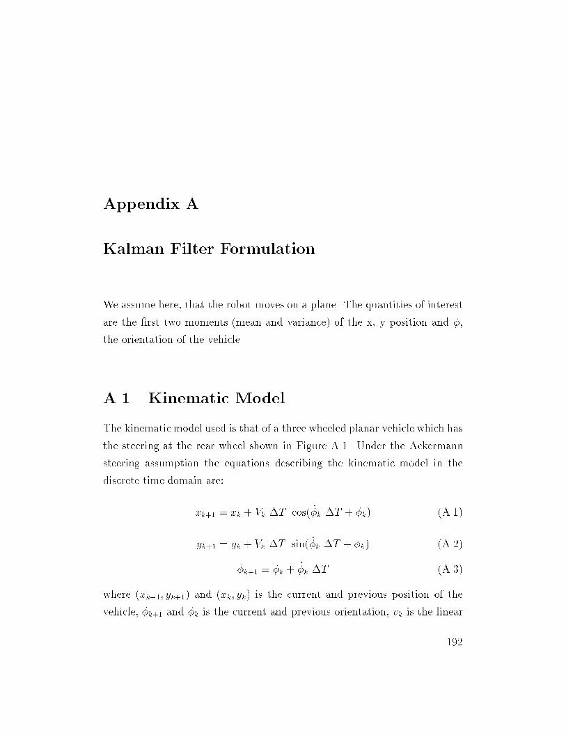
Appendix A
Kalman Filter Formulation
We assume here, that the robot moves on a plane. The quantities of interest
are the rst two moments (mean and variance) of the x, y position and ,
the orientation of the vehicle.
A.1 Kinematic Model
The kinematic model used is that of a three wheeled planar vehicle which has
the steering at the rear wheel shown in Figure A.1. Under the Ackermann
steering assumption the equations describing the kinematic model in the
discrete time domain are:
xk+1 = xk + Vk T cos( _k T + k) (A.1)
yk+1 = yk + Vk T sin( _k T + k) (A.2)
k+1 = k + _k T (A.3)
where (xk+1; yk+1) and (xk; yk) is the current and previous position of the
vehicle, k+1 and k is the current and previous orientation, vk is the linear
192
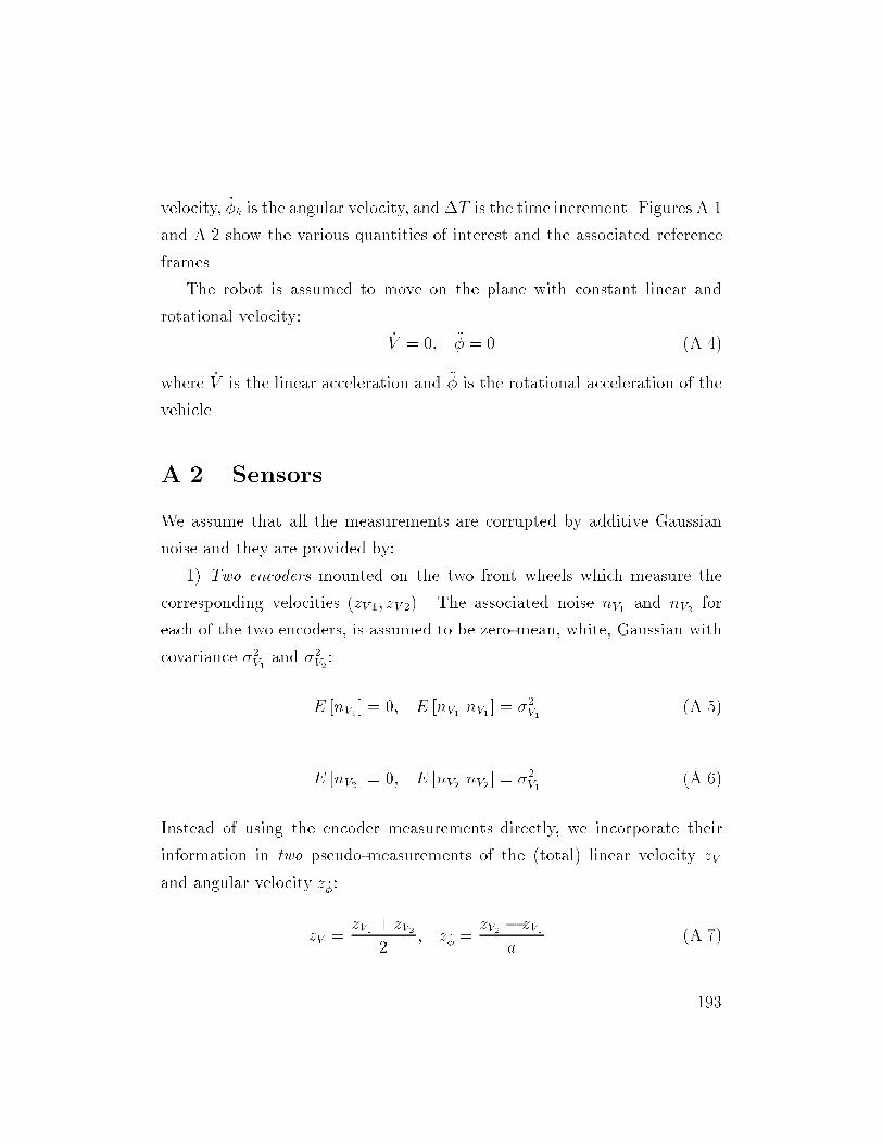
velocity, _k is the angular velocity, and T is the time increment. Figures A.1
and A.2 show the various quantities of interest and the associated reference
frames.
The robot is assumed to move on the plane with constant linear and
rotational velocity:
_V = 0; = 0 (A.4)
where _V is the linear acceleration and is the rotational acceleration of the
vehicle.
A.2 Sensors
We assume that all the measurements are corrupted by additive Gaussian
noise and they are provided by:
1) Two encoders mounted on the two front wheels which measure the
corresponding velocities (zV 1; zV 2). The associated noise nV1 and nV2 for
each of the two encoders, is assumed to be zero-mean, white, Gaussian with
covariance 2V1 and 2V2:
E [nV1] = 0; E [nV1 nV1] = 2V1 (A.5)
E [nV2] = 0; E [nV2 nV2] = 2V1 (A.6)
Instead of using the encoder measurements directly, we incorporate their
information in two pseudo-measurements of the (total) linear velocity zV
and angular velocity z _:
zV =zV1 + zV2
2; z _ =
zV2 zV1a
(A.7)
193
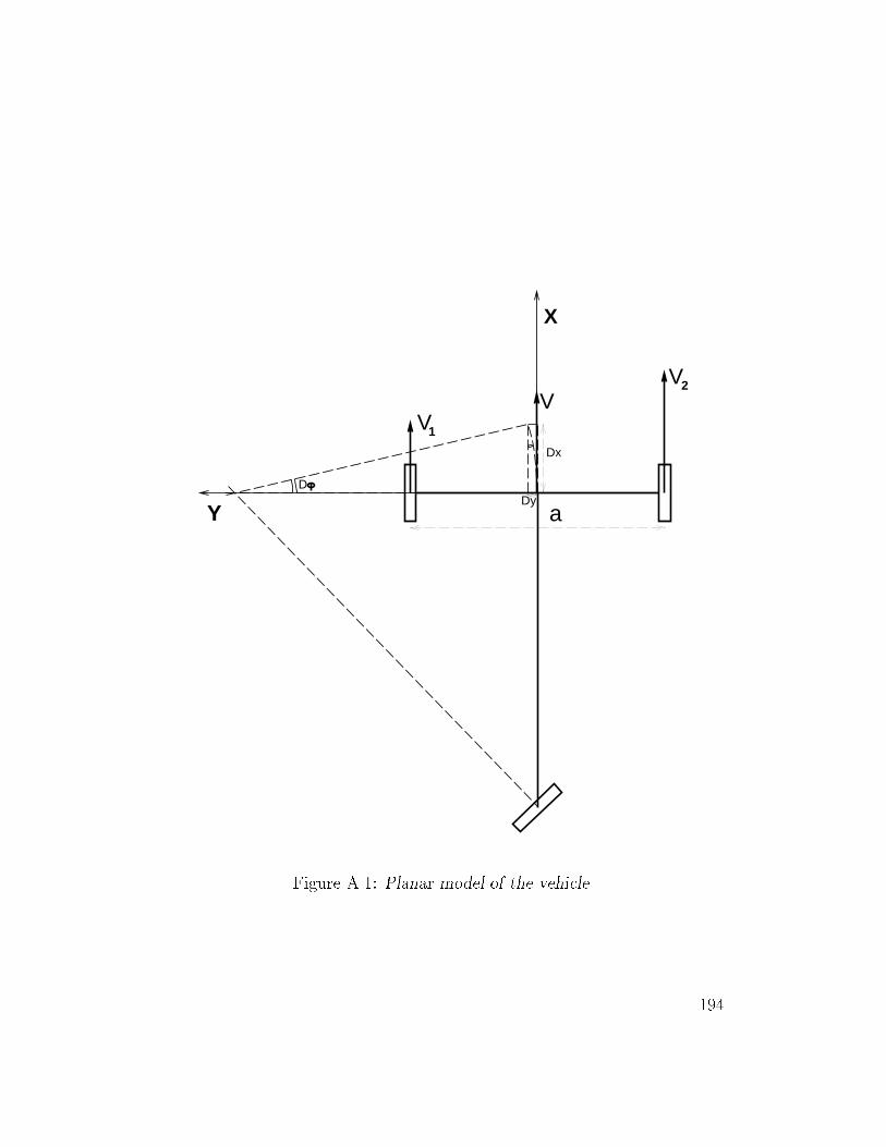
V
a
Dx
Dy
2V
1V
D
X
Y
Figure A.1: Planar model of the vehicle.
194
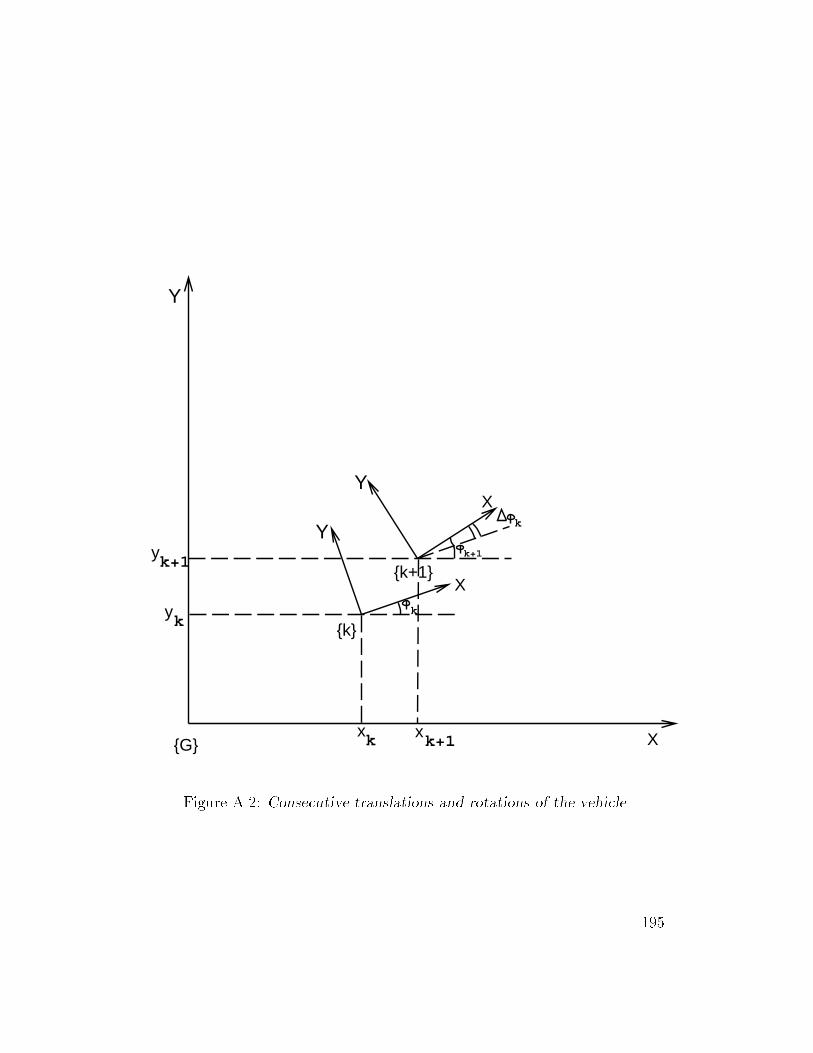
G
k
k+1
X
X
X
xk k+1x
yk
yk+1
k
k+1
k
Y
Y
Y
Figure A.2: Consecutive translations and rotations of the vehicle.
195
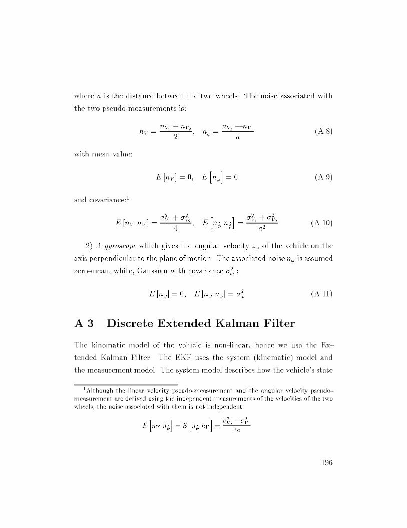
where a is the distance between the two wheels. The noise associated with
the two pseudo-measurements is:
nV =nV1 + nV2
2; n _ =
nV2 nV1a
(A.8)
with mean value:
E [nV ] = 0; Ehn _
i= 0 (A.9)
and covariance:1
E [nV nV ] =2V1 + 2V2
4; E
hn _ n _
i=
2V1 + 2V2a2
(A.10)
2) A gyroscope which gives the angular velocity z! of the vehicle on the
axis perpendicular to the plane of motion. The associated noise n! is assumed
zero-mean, white, Gaussian with covariance 2! :
E [n!] = 0; E [n! n!] = 2! (A.11)
A.3 Discrete Extended Kalman Filter
The kinematic model of the vehicle is non-linear, hence we use the Ex-
tended Kalman Filter. The EKF uses the system (kinematic) model and
the measurement model. The system model describes how the vehicle's state
1Although the linear velocity pseudo-measurement and the angular velocity pseudo-
measurement are derived using the independent measurements of the velocities of the two
wheels, the noise associated with them is not independent:
EhnV n _
i= E
hn _ nV
i=
2V2 2V12a
196
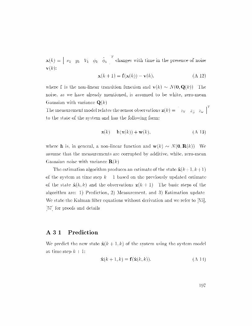
x(k) =hxk yk Vk k _k
iTchanges with time in the presence of noise
v(k):
x(k + 1) = f(x(k)) + v(k); (A.12)
where f is the non-linear transition function and v(k) N(0;Q(k)). The
noise, as we have already mentioned, is assumed to be white, zero-mean
Gaussian with variance Q(k).
The measurementmodel relates the sensor observations z(k) =hzV z _ z!
iTto the state of the system and has the following form:
z(k) = h(x(k)) +w(k); (A.13)
where h is, in general, a non-linear function and w(k) N(0;R(k)). We
assume that the measurements are corrupted by additive, white, zero-mean
Gaussian noise with variance R(k).
The estimation algorithm produces an estimate of the state x(k+1; k+1)
of the system at time step k + 1 based on the previously updated estimate
of the state x(k; k) and the observations z(k + 1). The basic steps of the
algorithm are: 1) Prediction, 2) Measurement, and 3) Estimation update.
We state the Kalman lter equations without derivation and we refer to [55],
[57] for proofs and details.
A.3.1 Prediction
We predict the new state x(k + 1; k) of the system using the system model
at time step k + 1:
x(k + 1; k) = f(x(k; k)): (A.14)
197
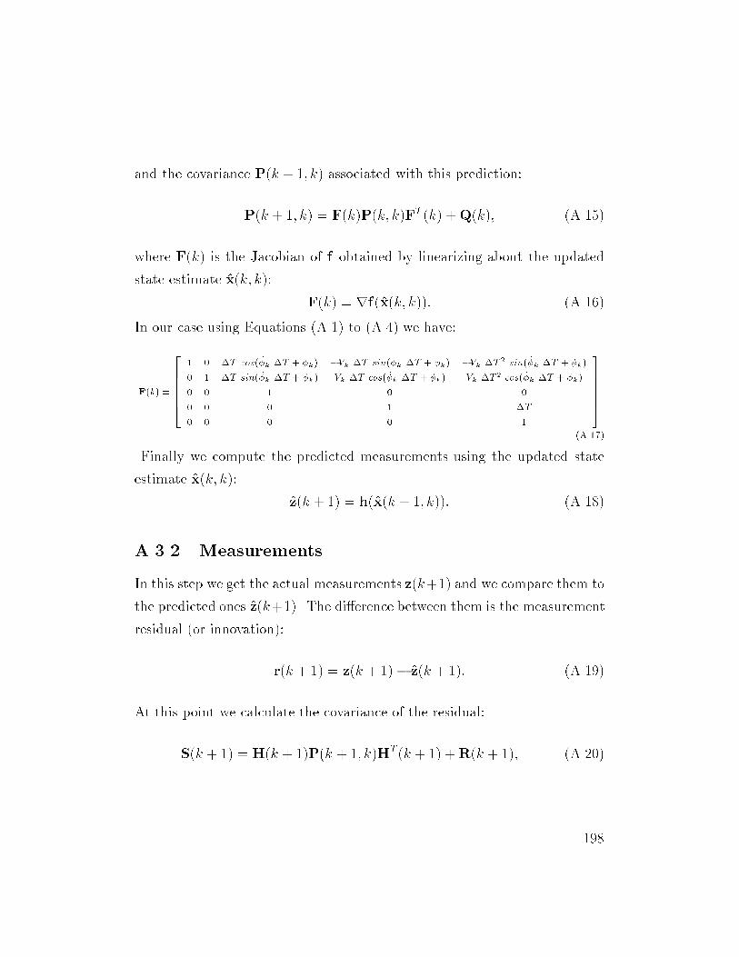
and the covariance P(k + 1; k) associated with this prediction:
P(k + 1; k) = F(k)P(k; k)FT (k) +Q(k); (A.15)
where F(k) is the Jacobian of f obtained by linearizing about the updated
state estimate x(k; k):
F(k) = rf(x(k; k)): (A.16)
In our case using Equations (A.1) to (A.4) we have:
F(k) =
266664
1 0 T cos( _k T + k) Vk T sin( _k T + k) Vk T 2 sin( _k T + k)
0 1 T sin( _k T + k) Vk T cos( _k T + k) Vk T 2 cos( _k T + k)
0 0 1 0 0
0 0 0 1 T
0 0 0 0 1
377775
(A.17)
Finally we compute the predicted measurements using the updated state
estimate x(k; k):
z(k + 1) = h(x(k + 1; k)): (A.18)
A.3.2 Measurements
In this step we get the actual measurements z(k+1) and we compare them to
the predicted ones z(k+1). The dierence between them is the measurement
residual (or innovation):
r(k + 1) = z(k + 1) z(k + 1): (A.19)
At this point we calculate the covariance of the residual:
S(k + 1) =H(k + 1)P(k + 1; k)HT (k + 1) +R(k + 1); (A.20)
198
where H(k + 1) is the Jacobian of h obtained by linearizing about the state
estimate x(k + 1; k):
H(k + 1) = rh(x(k + 1; k)) (A.21)
and which for our case is:
H(k + 1) =
266640 0 1 0 0
0 0 0 0 1
0 0 0 0 1
37775 (A.22)
A.3.3 Estimation update
In the last step of the estimation algorithm we use the measurement residual
r(k + 1) to correct the state prediction x(k + 1; k) and thus compute the
updated state estimate x(k + 1; k + 1). In order to do that we calculate the
Kalman gain:
W(k + 1) = P(k + 1; k)HT (k + 1)S1(k + 1); (A.23)
and then we update the state prediction:
x(k + 1; k + 1) = x(k + 1; k) +W(k + 1)r(k + 1): (A.24)
Finally we compute the associated covariance:
P(k + 1; k + 1) = P(k + 1; k)W(k + 1)S(k + 1)WT (k + 1): (A.25)
This is used as the new state covariance in the next iteration of the estimation
algorithm.
199
Appendix B
Quaternion Equations
B.1 Quaternion Kinematic Equations
In this section we dene:
~_true = ~!m ~btrue ~nr (B.1)
~_i = ~!m ~bi (B.2)
We also repeat Equations (5.15), (5.11) and (5.12):
q = qtrue q1i (B.3)
d
dtA(t) =
hh~!(t)
iiA(t) (B.4)
d
dtq(t) =
1
2(~!(t))q(t) (B.5)
which we use to prove Equation (5.20):
d
dt~q =
hh~!m
ii~q
1
2(~b+ ~nr) (B.6)
200
First we rewrite Equation (B.3) in terms of the corresponding attitude ma-
trices as:
A(q) = A(qtrue q1i ) = A(qtrue)A(q1i ) (B.7)
dierentiating with respect to time we have:
d
dtA(q) =
d
dt(A(qtrue))A(q
1i ) +A(qtrue)
d
dt(A(q1i )) (B.8)
From
1 = qi q1i (B.9)
we have
I33 = A(qi q1i ) = A(qi)A(q1i ) (B.10)
which with dierentiation with respect to time gives:
d
dt(A(qi))A(q
1i ) +A(qi)
d
dt(A(q1i )) = 0 (B.11)
ord
dt(A(q1i )) = A1(qi)
d
dt(A(qi))A(q
1i ) (B.12)
or by using A1(qi) = A(q1i )
d
dt(A(q1i )) = A(q1i )
d
dt(A(qi))A(q
1i ) (B.13)
Substituting in Equation (B.8), Equation (B.13) we have:
d
dtA(q) =
d
dt(A(qtrue))A(q
1i )A(qtrue)A(q
1i )
d
dt(A(qi))A(q
1i ) (B.14)
201
or by using Equation (B.4) with the appropriate rotational velocity vectors:
d
dtA(q) =
~_true
A(qtrue)A(q
1i )A(qtrue)A(q
1i )
~_i
A(qi)A(q
1i )
(B.15)
Combining the matrix products we have:
d
dtA(q) =
~_true
A(qtrue q1i )A(qtrue q1i )
~_i
A(qi q1i )
(B.16)
ord
dtA(q) =
~_true
A(q)A(q)
~_i
(B.17)
The previous equation written in quaternion form is:
d
dtq =
1
2(
24 ~_true
0
35 q q
24 ~_i
0
35) (B.18)
which using Equations (B.1) and (B.2) becomes:
d
dtq =
1
2(
24 ~!m ~btrue ~nr
0
35 q q
24 ~!m ~bi
0
35) (B.19)
or
d
dtq =
1
2(
24 ~!m
0
35 q q
24 ~!m
0
35) 1
2(
24 ~btrue + ~nr
0
35 q q
24 ~bi
0
35)
(B.20)
At this point we need to use a more compact form of combining two quater-
nion vectors. If
a =
24 ~a
a0
35 ; b =
24 ~b
b0
35 ; (B.21)
202
then
a b =
24 a0~b+ b0~a ~a~b
a0b0 ~aT ~b
35 (B.22)
Applying these in the rst term of Equation (B.20) we have:
24 ~!m
0
35
24 ~q
q4
35
24 ~q
q4
35
24 ~!m
0
35 =
24 ~!mq + 0 ~q ~!m ~q
0 q4 ~! Tm ~q
35
24 ~q 0 + q4 ~!m ~q ~!m
q4 0 ~q T ~!m
35 =
2
24 ~!m ~q
0
35 (B.23)
Similarly the second part of Equation (B.20) can be written as:
24 ~btrue + ~nr
0
35
24 ~q
q4
35
24 ~q
q4
35
24 ~bi
0
35 =
24 0 ~q + q4(~btrue + ~nr) (~btrue + ~nr) ~q
0 q4 (~btrue + ~nr)T~q
35
24 q4 ~bi + 0 ~q ~q ~bi
q4 0 ~q T ~bi
35 =
24 q4(~btrue ~bi + ~nr) (~btrue ~bi + ~nr) ~q
(~btrue ~bi + ~nr)T~q
35 =
24 q4 ~! ~! ~q
~! T ~q
35 =
203
=
24 ~!
0
35 q4
24 ~! ~q
~! T ~q
35 (B.24)
where
~! = ~btrue ~bi + ~nr = ~b+ ~nr (B.25)
For very small rotations we can assume that q4 ' 1 and thus Equation
(B.24) can be simplied as:
24 ~btrue + ~nr
0
35
24 ~q
q4
35
24 ~q
q4
35
24 ~bi0
35 '
24 ~!
0
35 (j~!j j~qj) '
24 ~!
0
35
(B.26)
Now substituting Equations (B.23) and (B.26) in Equation (B.20) we have:
d
dt
24 ~q
q4
35 = 1
2(2)
24 ~!m ~q
0
35+ 1
2
24 ~!
0
35 =
24hh
~!mii
~q
0
35+ 1
2
24 ~!
0
35
(B.27)
Separating the vector from the scalar terms the previous equation is described
by:d
dt~q =
hh~!m
ii~q
1
2(~b+ ~nr) (B.28)
andd
dtq4 = 0 (B.29)
204
B.2 Quaternion Dierence Equations
Here we use an equivalent expression for the denition of the quaternion
product (combination). This is:
q q = fqgq0 =
26666664
q4 q3 q2 q1
q3 q4 q1 q2
q2 q1 q4 q3
q1 q2 q3 q4
37777775
26666664
q01
q02
q03
q04
37777775 (B.30)
or
q q = fqgq0 =h(q) q
iq0 (B.31)
It can easily be shown that:
T (q)(q) = jqj2I33 = I33 (B.32)
since jqj2 = 1 for unit quaternions, and that:
(q)T(q) = jqj2I44 qq T (B.33)
T (q)q = 033 (B.34)
Applying Equation (B.31) to the denition of q we have:
qtrue = q qi =h(qi) qi
iq =
h(qi) qi
i 24 ~q
q4
35 (B.35)
or
qtrue = (qi)~q + qiq4 (B.36)
205
Multiplying both sides with T (qi) we have:
T (qi)qtrue = T (qi)(qi)~q+ T (qi)qiq4 (B.37)
Substituting from Equations (B.32) and (B.34) we have:
~q = T (qi)qtrue (B.38)
Now starting from Equations (B.36) and (B.38)
qtrue = (qi)~q+ qiq4 = (qi)T (qi)qtrue + qiq4 (B.39)
and using Equation (B.33)
qtrue = (I44 qiqTi )qtrue + qiq4 = qtrue qiq
Ti qtrue + qiq4 (B.40)
or
qiq4 = qiqTi qtrue (B.41)
from which we conclude that:
q4 = qTi qtrue (B.42)
At this point we augment Equation (B.38) with the bias to get:
24 T (qi) 033
034 I33
3524 qtrue~btrue
35 =
24 ~q
~btrue
35 (B.43)
206
Also from Equation (B.34) we can similarly write:
24 T (qi) 033
034 I33
3524 qi~bi
35 =
24 031
~bi
35 (B.44)
Subtracting the last two equations we have:
24 T (qi) 033
034 I33
3524 qtrue qi~btrue ~bi
35 =
24 ~q
~btrue ~bi
35 (B.45)
or 24 ~q
~b
35 =
24 T (qi) 033
034 I33
3524 q
~b
35 = ST (qi)
24 q
~b
35 (B.46)
where
S(qi) =
24 (qi) 043
033 I33
35 (B.47)
Notice that
S(qi)ST (qi) =
24 (qi) 043
033 I33
3524 T (qi) 033
034 I33
35 =
=
24 (qi)
T (qi) 043
034 I33
35 =
24 I44 043
034 I33
35 (B.48)
or
S(qi)ST (qi) = I77 (B.49)
207

Multiplying both sides of Equation (B.46) with S(qi) and applying Equation
(B.49) we get
S(qi)
24 ~q
~b
35 = S(qi)S
T (qi)
24 q
~b
35 (B.50)
or 24 q
~b
35 = S(qi)
24 ~q
~b
35 (B.51)
In order to compute the relation between the covariances of the (error) quan-
tities x =
24 q
~b
35 and x =
24 ~q
~b
35 we substitute Equations (B.46) and
(B.51) in the following expectations used for their denition:
P77 = Ehx xT
i= E
hS(qi) x xT ST (qi)
i=
= S(qi) Ehx xT
iST (qi) = S(qi) P66 S
T (qi) (B.52)
Similarly
P66 = Ehx xT
i= E
hST (qi) x xT S(qi)
i=
= ST (qi) Ehx xT
iS(qi) = ST (qi) P77 S(qi) (B.53)
208
Appendix C
Perfect Relative Pose Measurement
In this section we examine the case where two robots meet (for example
robots 2 and 3) and measure their relative position and orientation (pose)
using some ideal perfect sensor. In this case, R23(tk+1) in Equation (6.17) is
zero, since the measurement is assumed to be perfect and therefore:
S(tk+1) = H23(tk+1)P (tk+1)H
T23(tk+1) +R23(tk+1) = H23(tk+1)P (t
k+1)H
T23(tk+1)
=h0 I I
i26664P11(t
k+1) P12(t
k+1) P13(t
k+1)
P21(tk+1) P22(t
k+1) P23(t
k+1)
P31(tk+1) P32(t
k+1) P33(t
k+1)
3777526664
0
I
I
37775
= P22(tk+1) P32(t
k+1) P23(t
k+1) + P33(t
k+1) (C.1)
Applying this to the covariance update equation (Equation (6.24)) we have:
P (t+k+1) = P (tk+1) P (tk+1)HT23(tk+1)S
1(tk+1)H23(tk+1)P (tk+1) =
209
= P (tk+1)
26664P11(t
k+1) P12(t
k+1) P13(t
k+1)
P21(tk+1) P22(t
k+1) P23(t
k+1)
P31(tk+1) P32(t
k+1) P33(t
k+1)
3777526664
0
I
I
37775S1(tk+1)
h0 I I
i26664P11(t
k+1) P12(t
k+1) P13(t
k+1)
P21(tk+1) P22(t
k+1) P23(t
k+1)
P31(tk+1) P32(t
k+1) P33(t
k+1)
37775 =
= P (tk+1)
26664P12(t
k+1) P13(t
k+1)
P22(tk+1) P23(t
k+1)
P32(tk+1) P33(t
k+1)
37775S1(tk+1)
h(P21(t
k+1) P31(t
k+1)) (P22(t
k+1) P32(t
k+1)) (P23(t
k+1) P33(t
k+1))
i(C.2)
The previous equation for the centralized system can be decomposed into
the following 9 equations:
P11(t+k+1) = P11(t
k+1)P12(t
k+1) P13(t
k+1)S1(tk+1)
P21(t
k+1) P31(t
k+1)(C.3)
P12(t+k+1) = P12(t
k+1)P12(t
k+1) P13(t
k+1)S1(tk+1)
P22(t
k+1) P32(t
k+1)(C.4)
P13(t+k+1) = P13(t
k+1)P12(t
k+1) P13(t
k+1)S1(tk+1)
P23(t
k+1) P33(t
k+1)(C.5)
P21(t+k+1) = P21(t
k+1)P22(t
k+1) P23(t
k+1)S1(tk+1)
P21(t
k+1) P31(t
k+1)(C.6)
P22(t+k+1) = P22(t
k+1)P22(t
k+1) P23(t
k+1)S1(tk+1)
P22(t
k+1) P32(t
k+1)(C.7)
P23(t+k+1) = P23(t
k+1)P22(t
k+1) P23(t
k+1)S1(tk+1)
P23(t
k+1) P33(t
k+1)(C.8)
210
P31(t+k+1) = P31(t
k+1)P32(t
k+1) P33(t
k+1)S1(tk+1)
P21(t
k+1) P31(t
k+1)(C.9)
P32(t+k+1) = P32(t
k+1)P32(t
k+1) P33(t
k+1)S1(tk+1)
P22(t
k+1) P32(t
k+1)
(C.10)
P33(t+k+1) = P33(t
k+1)P32(t
k+1) P33(t
k+1)S1(tk+1)
P23(t
k+1) P33(t
k+1)
(C.11)
Theorem 1 Consider the previous covariance update equations for the cen-
tralized system (pose estimator) for the 3 robots when two of them meet,
robots 2 and 3, and measure their relative pose perfectly. Assume that P12(tk+1) 6=
P13(tk+1) , P21(t
k+1) 6= P31(t
k+1), P22(t
k+1) 6= P23(t
k+1) , P22(t
k+1) 6=
P32(tk+1), P32(t
k+1) 6= P33(t
k+1) , P23(t
k+1) 6= P33(t
k+1) such that S(tk+1)
in Equation (C.1) is not 0. Then the covariances of the two meeting robots
are equal and they are also equal to their cross-correlation terms. That is:
P22(t+k+1) = P33(t
+k+1) = P23(t
+k+1) = P32(t
+k+1).
We will prove the following:
1. P33(t+k+1) = P32(t
+k+1)
2. P22(t+k+1) = P32(t
+k+1)
3. P22(t+k+1) = P23(t
+k+1)
1.
P33(t+k+1) = P32(t
+k+1),
P33(tk+1)
hP32(t
k+1) P33(t
k+1)
iS1(tk+1)
hP23(t
k+1) P33(t
k+1)
i=
P32(tk+1)
hP32(t
k+1) P33(t
k+1)
iS1(tk+1)
hP22(t
k+1) P32(t
k+1)
i,
211
P32(tk+1) P33(t
k+1) =
hP32(t
k+1) P33(t
k+1)
iS1(tk+1)
hP22(t
k+1) P32(t
k+1) P23(t
k+1) + P33(t
k+1)
i,
P32(tk+1) P33(t
k+1) =
hP32(t
k+1) P33(t
k+1)
iS1(tk+1)S(tk+1),
P32(tk+1) P33(t
k+1) = P32(t
k+1) P33(t
k+1) (C.12)
2.
P22(t+k+1) = P32(t
+k+1),
P22(tk+1)
hP22(t
k+1) P23(t
k+1)
iS1(tk+1)
hP22(t
k+1) P32(t
k+1)
i=
P32(tk+1)
hP32(t
k+1) P33(t
k+1)
iS1(tk+1)
hP22(t
k+1) P32(t
k+1)
i,
P22(tk+1) P32(t
k+1) =
hP22(t
k+1) P23(t
k+1) P32(t
k+1) + P33(t
k+1)
iS1(tk+1)
hP22(t
k+1) P32(t
k+1)
i,
P22(tk+1) P32(t
k+1) = S(tk+1)S
1(tk+1)hP22(t
k+1) P32(t
k+1)
i,
P22(tk+1) P32(t
k+1) = P22(t
k+1) P32(t
k+1) (C.13)
212
3.
P22(t+k+1) = P23(t
+k+1), P T
22(t+k+1) = P T
23(t+k+1), P22(t
+k+1) = P32(t
+k+1)
(C.14)
Theorem 2 Consider the previous covariance update equations for the cen-
tralized system (pose estimator) for the 3 robots when two of them meet,
robots 2 and 3, and measure their relative pose perfectly. Assume that P12(tk+1) 6=
P13(tk+1) , P21(t
k+1) 6= P31(t
k+1), P22(t
k+1) 6= P23(t
k+1) , P22(t
k+1) 6=
P32(tk+1), P32(t
k+1) 6= P33(t
k+1) , P23(t
k+1) 6= P33(t
k+1) such that S(tk+1)
in Equation (C.1) is not 0. Then the cross-correlation terms between the third
robot and the two meeting robots are equal. That is: P21(t+k+1) = P31(t
+k+1)
and P12(t+k+1) = P13(t
+k+1).
1.
P21(t+k+1) = P31(t
+k+1),
P21(tk+1)
hP22(t
k+1) P23(t
k+1)
iS1(tk+1)
hP21(t
k+1) P31(t
k+1)
i=
= P31(tk+1)
hP32(t
k+1) P33(t
k+1)
iS1(tk+1)
hP21(t
k+1) P31(t
k+1)
i,
P21(tk+1) P31(t
k+1) =
hP22(t
k+1) P23(t
k+1) P32(t
k+1) + P33(t
k+1)
iS1(tk+1)
hP21(t
k+1) P31(t
k+1)
i,
P21(tk+1) P31(t
k+1) = S(tk+1)S
1(tk+1)hP21(t
k+1) P31(t
k+1)
i,
213

P21(tk+1) P31(t
k+1) = P21(t
k+1) P31(t
k+1) (C.15)
2.
P12(t+k+1) = P13(t
+k+1), P T
12(t+k+1) = P T
13(t+k+1), P21(t
+k+1) = P31(t
+k+1)
(C.16)
214