Observational Tests of World Models - Caltech …george/ay21/readings/... · radiation itself, ... the observed World picture to the World map ... and ~. ~ ~ = = OBSERVATIONAL TESTS

Ann. Rev. Astron. Astrophys. 1988. 26: 561~530Copyright © 1988 by Annual Reviews Inc. All rights reserved

OBSERVATIONAL TESTS OFWORLD MODELS

Allan Sandage

Department of Physics and Astronomy, The Johns Hopkins University,Baltimore, Maryland 21218 and Space Telescope Science Institute,3700 San Martin Drive, Baltimore, Maryland 212181

1. THE ELEMENTS OF PRACTICAL COSMOLOGY

The standard model of cosmology, based on what has come to be calledthe Friedmann-Lemaitre-Robertson-Walker (FLRW) model (hereinaftersimply the Friedmann model), is now part of scientific culture. The mostpopular current version leads to the hot big bang (HBB) description events near the beginning of the cosmic expansion, which has often beencalled a creation2 moment at the beginning of physical time. In this reviewa prejudice in favor of the HBB [in contrast to cold beginnings discussed,for example, by Layzer (1987) in his remarkable book on the growth order in the Universe] can hardly be suppressed, successful as the modelhas become in providing an understanding of the abundance of He4 andthe 3-K radiation. Nevertheless, if a description of beginnings in this senseis to be confined within the methods of science rather than to be coloredby teleological metaphysics, the model must pass the tests normal toscience rather than to be accepted as revealed truth. The purpose of this

~ Presently at Mount Wilson Observatory of the Carnegie Institution of Washington, 813Santa Barbara Street, Pasadena, California 91101.

~ Creation is a flammable word that triggers responses often not intended by writers whouse it. Gamow, in reply to a critic who complained about the title of his famous book "TheCreation of the Universe," advised his reader to interpret creation as something similar to alady’s fashion rather than to misinterpret it as a theological statement. If it were the latter,the inquiry would be removed from the possibility of using the scientific method to discover,rather than some other method to reveal. When creation is used in this review, its meaningis in the Gamow sense. Nevertheless, the subject is possibly as close as science can come tothe questions of origins--hence its enormous appeal.

5610066-4146/88/0915-0561 $02.00

www.annualreviews.org/aronlineAnnual Reviews

Ann

u. R

ev. A

stro

. Ast

roph

ys. 1

988.

26:5

61-6

30. D

ownl

oade

d fr

om a

rjou

rnal

s.an

nual

revi

ews.

org

by C

alif

orni

a In

stitu

te o

f T

echn

olog

y on

04/

10/0

9. F

or p

erso

nal u

se o

nly.

http://www.annualreviews.org/aronline

562 SANDAGE

review is to discuss the direct tests of observation that lead to the viewthat a hot beginning to a current universe of finite age did occur.

Reviews of the theoretical aspects of the FLRW standard model fromvarious viewpoints have appeared previously in this series. Novikov &Zeldovich (1967) surveyed the physical aspects of the HBB early Universe.Harrison (1973) summarized and discussed the various chemical eras,starting from a presumed initial singularity of very high temperature tothe time of decoupling of matter and radiation, with the consequent for-mation of atoms some 30,000 yr after the Creation. Steigrnan (1976)reviewed the evidence and the reason(s) for the present matter-antimatterasymmetry. Boesgaard & Steigrnan (1985) discussed the theory and com-pared its predictions with observations of big bang nucleosynthesis. Thiscomparison of the observed abundances of H, D, He3, He4, and Li7 withthe calculations provides one of the two most powerful proofs of the HBBmodel. The other, of course, is the 3-K microwave background (MWB)radiation itself, discussed in these Reviews by Sunyaev & Zeldovich (1980)from the theoretical standpoint, and by Thaddeus (1972) and Weiss (1980)from the observational. The spectrum of the radiation resembles closelythat of a blackbody. This is an important argument supporting a relicorigin for the radiation, although alternate explanations have been pro-posed (Hoyle et al. 1968, Layzer & Hively 1973, Rana 1981, and referencestherein).

Other theoretical aspects of the standard model have been developed inthese pages by Gould (1968) and Field (1972) in their reviews of intergalactic medium, by Gott (1977) in his discussion of galaxy formation,and by Ellis (1984) in his survey of alternatives to the HBB standardmodel.

Particularly useful among the many workshop and conference pro-ceedings that give entrance to the extensive archive literature are PhysicalCosrnolo~Ty (Balian et al. 1979), Astrophysical CosmolotTy (Bruck et al.1982), Proyress in CosmolotTy (Wolfendale 1981), Cosmoloyy and Fun-damental Physics (Setti & Van Hove 1983), and Inner Space/Outer Space(Kolb et al. 1986).

Most of these discussions center on theoretical consequences of the HBBmodel. There have been only a few systematic reviews of results of theseveral direct (mostly geometrical) tests of the model. To be sure, impor-tant expositions of the principles of some of the classical tests are containedin discussions of the general properties of the models, such as the foun-dational reviews by Robertson (1933, 1955), the comprehensive summaryby Zeldovich (1965), the lectures by Gunn (1978), and the textbooksby McVittie (1965), Peebles (1971), Weinberg (1972), Rowan-Robinson(1981), Narlikar (1983), and Zeldovich & Novikov (1983). But in


Ann

u. R

ev. A

stro

. Ast

roph

ys. 1

988.

26:5

61-6

30. D

ownl

oade

d fr

om a

rjou

rnal

s.an

nual

revi

ews.

org

by C

alif

orni

a In

stitu

te o

f T

echn

olog

y on

04/

10/0

9. F

or p

erso

nal u

se o

nly.


OBSERVATIONAL TESTS OF WORLD MODELS 563

these accounts, details of the practical methods of the subject are kept asa black art, taken to be known, and therefore not set out in detail.

The present review is concerned with the observational aspects of thesubject. This is because no textbook now exists on what every studentshould know if practical cosmology--the linchpin of the laboratory partof the subject--is to become their way of life. The emphasis is on thedetails of the calculations (i.e. the equations) that are necessary to makecomparisons between the models and the data. My aim is to assess criticallyif the model does in fact have experimental verification beyond the admit-tedly very powerful tests of the Gamow, Alpher, and Herman 3-Kradiation, and the consequent predictions of baryon and nucleosynthesisout of the HBB.

The most satisfactory outcome of any such test would be some directverification of the curvature of space by an experimental 9eometricalmeasurement similar to those proposed by Gauss and by Karl Schwarz-schild. Spatial curvature is required by the foundation of the theory, deeplyburied as it is in the covering theory of general relativity (Section 2).Barring such a test (none has yet been successful), a direct verification thatthe redshift is due to a true expansion of the geometrical manifold wouldbe most helpful, but again such a demonstration is not quite available yet(see Section 8).

One precise prediction of the theory is that the form of the redshift-distance relation [observed at fixed cosmic time--i.e, found by reducingthe observed World picture to the World map (in the language of Milne)to account for the light travel time] be strictly linear, not exponential asin a "tired light" theory, nor in any other form as in some nonstandardmodels. Tests of the linearity of the redshift vector field are singularlyrobust and are featured later in this review.

One of the central requirements of the standard model is that the timesince the Creation (defined here as the beginning of physical time) related to the observed Hubble expansion rate Hb-1 by a factor thatdepends on the density parameter f~0 (in principle observable) via theconnection (dictated by relativity) between the matter density and thespace-time curvature. This relation is kc2/R2= H~o(f~o- 1) if the cos-mological constant A is zero. Otherwise, the curvature has the additionalterm of Ac2/3 added. This test of the time scale, made by comparing thetheoretical value of the age of the Universe, To = H~- ~f(D,0, A), with otherclocks set ticking at the singularity, must work if the standard model is tobe an adequate description. Because the test is so powerful, it has achance to give a bona fide scientific judgment, if the relevant times can beaccurately measured. We consider this test at length later in this review.

Finally, it is a commonplace that if any model is correct, it must have


Ann

u. R

ev. A

stro

. Ast

roph

ys. 1

988.

26:5

61-6

30. D

ownl

oade

d fr

om a

rjou

rnal

s.an

nual

revi

ews.

org

by C

alif

orni

a In

stitu

te o

f T

echn

olog

y on

04/

10/0

9. F

or p

erso

nal u

se o

nly.


564 SANDAGE

verifiable predictive power. The HBB ideas would seem to have alreadypassed the high hurdle of the 3-K MWB radiation first predicted byGamow (1946, 1948) and his fellow "originalists" (Alpher 1948, Alpheret al. 1948, 1953, Alpher & Herman 1948, 1950) and later required byPeebles (1986), Wagoner et al. (1967), Wagoner (1973), and now so others. The radiation was subsequently discovered by Penzias & Wilson0965). At the time, Dicke et al. 0965) were engaged in a search whosepurpose was in fact to verify their independent prediction as a requirementof a hot big bang.

The most elementary prediction of any model that does not postulatecontinuous creation is that the mean contents of the Universe (suitablyspatially averaged) were once younger than they are now. Verification ofthis required evolution in the look-back time is yet nascent. The variety ofobservational tests using galaxies at different redshifts, i.e. at differentlook-back times, give suggestive but not yet quite overwhelming evidencefor evolution with time (see Section 7).

In the sections that follow I assume no detailed familiarity with thetheoretical literature, nor familiarity at all with the observations. Wedevelop the necessary apparatus for the tests as we need them so as to laybare the assumptions upon which they rest. The level is aimed at first-year graduate students to provide them entrance to the literature for thenecessary data, equations, and correction tables.

The menu for this journey through the test maze begins with the simplestgeometrical predictions of curved space. Here the galaxy number count-distance test is set out in its most direct form of the volume V(r) enclosedwithin the "distance" l between us and coordinate point r in the comovingmanifold (defined in the next section). Because the l distances are neededbut are not themselves measured by rigid rods (suitably defined), introduce next the distance-redshift relation that follows from the require-ments of homogeneity and isotropy of the Roberts0n-Walker spaces. Thisleads naturally to the line element with its magic of accounting for thelight-travel-time effects by using the null geodesic equation for light rays.This, in turn, permits direct entry to the redshift-distance equations, andtherefrom to the redshift-luminosity (Mattig) relations for standardcandles. This is the Hubble diagram straightaway. The practical details ofcorrections for aperture effect, K dimming, cluster richness, and the Bautz-Morgan contrast correlation are then set out. It is from the Hubble diagramfor cluster galaxies that the linearity test for the form of the velocity fieldis most directly made.

Armed now with the re(z, qo) Mattig equation, the N(z, qo) count-redshiftrelation (as a function of space curvature) can be transformed to theobserved N(m, qo) predictions, integrating over the luminosity function. It


Ann

u. R

ev. A

stro

. Ast

roph

ys. 1

988.

26:5

61-6

30. D

ownl

oade

d fr

om a

rjou

rnal

s.an

nual

revi

ews.

org

by C

alif

orni

a In

stitu

te o

f T

echn

olog

y on

04/

10/0

9. F

or p

erso

nal u

se o

nly.



is the comparison of this prediction with the observed N(m) relationthat motivated Hubble to claim a geometrical measurement of the spacecurvature (Section 5).

These developments dispose, then, of the N(m, qo) and the 0/(2, q0) tests,which are half of the four classical hopes (Sandage 1961a) to find the oneWorld model.

The remaining two tests are the angular size-redshift relation, and thetime-scale comparison. The angular size variation with redshift shouM bethe most direct way to sample the geometry (Hoyle 1959). The theory this test leads to the surface brightness ~ (1 +z)-4 relation, which must bevalid if the expansion is real. Success in performing the experiment centersabout the use of metric rather than isophotal galaxy diameters. The searchfor a suitable measure of a metric size is the present stumbling block, oneyet to be adequately dislodged, but progress has been made (Section 8).

The time-scale test depends on the value of the Hubble expansion rateH0. The problems of its determination in the presence of observationalbias in the data samples are set out in Section 9, where evidence favoringthe long distance scale, which requires a low value of H0, is discussed.

2. EXPERIMENTAL GEOMETRY

2.1 The Necessity for Space Curvature

Is space curvature real? As an experimental problem, it becomes an epis-temological question because of ambiguities in the definitions concerningthe nature of the measuring rods and the character of the distancesobtained with them (Section 2.2). As a theoretical problem, the reality ofthe formalism in the present physics (Einstein’s theory of gravity) must sought.

The non-Euclidean geometry, foreshadowed by Saccheri3 and inventedby Gauss, Bolyai, and Lobachevski, was largely a curiosity for mostscientists in the mid-nineteenth century, despite its central importance inthis century, lying at the root of our present understanding of space-time.Unlike Saccheri, Gauss believed in its reality and proposed methods to

3 The grip that our intuition holds on the mind concerning the unreality of non-Euclideangeometry prevented Saccheri from believing what his reason had discovered. E. T. Bell, inhis book Development of Mathematics, writes, "[Saccheri’s] brilliant failure is one of themost remarkable instances in the history of inathematical thought of the mental inertiainduced by an education in obedience and orthodoxy, confirmed in mature life by an excessivereverence for the perishable works of the immortal dead [Euclid]. With two geometries, eachas valid as Euclid’s in his hand, Saccheri threw both away because he was willfully determinedto continue in the obstinate worship of his idol, despite the insistent promptings of his ownsane reason."


Ann

u. R

ev. A

stro

. Ast

roph

ys. 1

988.

26:5

61-6

30. D

ownl

oade

d fr

om a

rjou

rnal

s.an

nual

revi

ews.

org

by C

alif

orni

a In

stitu

te o

f T

echn

olog

y on

04/

10/0

9. F

or p

erso

nal u

se o

nly.


566 SAbIDAGE

measure the spatial curvature. K. $chwarzschild began such measurementsby putting limits on the value of the curvature using the distribution ofstellar parallaxes.

The intuitive geometry that is fixed on the senses by that outside spatialframe which gives us our ordinary experience seems Euclidean. Areasincrease strictly as r~, volumes as r3, using the apparently common-sensedefinition of r. The concept of spatial curvature is foreign to the intuitionand unreal to the nonscientist.

Nevertheless, if we take the structure of general relativity as definin9reality, matter really does curve space. Particles move on straight lines incurved space instead of on curved paths in straight space. To be sure, wetrade one mystery for another. The 9~’s of the geometrical metric aredetermined by the distribution of matter, replacing Newton’s force at adistance with geodesics in curved space. It is in this sense that generalrelativity has geometrized dynamics. The question remains, Is the cur-vature "real?" But what is reality? Indeed, has the question any verifiablemeaning?

As an arguable definition, we could try "for X to be real requires thatX have effects. ’’4 If we observe unmistakable effects we would say the thing"causing them" is real. It was the absence of predicted effects that removedthe ether from reality. It was the verification of many predictions ofits consequences that made the Lorentz transformation "real." Yet theFitzgerald contraction as one "explanation" of the transformation is notreal in this sense, but the time dilatation debatably is (Kennedy & Thorn-dike 1932), because it is observed, making the relativity of space-timeequally real as long as no other explanation is possible.

On this definition space-time curvature is real. The predictions of itseffects via Einstein’s equations are well verified [see Will (1981) and Backer& Hellings (1986) for recent reviews]. The curvature is measured by thenon-Euclidean tT~’s. Yet areas and volumes are not measured. What actu-ally is verified is that the formalism of the equations works in certainexperimental circumstances (advance of Mercury’s perihelion, timedilatation, a ray bending about the Sun, gravitational radiation, and per-haps even gravitational lensing).

However, the presence of space curvature would be more convincing ifwe had a simple direct proof that volumes fail to increase as r3, or that the

4 This is similar to but not identical with a wider definition often used that "X is real if it

is an essential element of a strongly confirmed theory." However, with both these definitions,a reality of this kind is ephemeral. If the theory is later found to be inadequate and must bereplaced, the "reality" associated with it must also be replaced, and hence was not real inthe ordinary usage of that word.


Ann

u. R

ev. A

stro

. Ast

roph

ys. 1

988.

26:5

61-6

30. D

ownl

oade

d fr

om a

rjou

rnal

s.an

nual

revi

ews.

org

by C

alif

orni

a In

stitu

te o

f T

echn

olog

y on

04/

10/0

9. F

or p

erso

nal u

se o

nly.



angular sizes of rods fail to decrease as r-1 in circumstances where theRiemann-Gauss scalar curvature, kc2/R2, is expected to be nonzero. Thefull problem of defining relevant distances in the cosmology of ideal(congruent) spaces then becomes the central point in deciding the realityof space curvature.

2.2 The Idea of Geometrical Experiments

How then are we to measure deviations from Euclidean predictions? Whatrules concerning the properties of measuring rods do we adopt, and bywhat rules do we assess whether an experiment has given a non-Euclideanresult? Early on, Poincar6 denied the reality of actual curved space bystating that in any measurement that appeared to give a non-Euclideanresult, one is at liberty to redefine the properties of the measuring rods insuch a way as to recover a Euclidean prediction. A particularly interestingexample of this, involving nonuniformly heated metal measuring rods, isgiven by Robertson (1949). Poincar6’s point has been variously debated(cf. Whittaker 1958, Reichenbach 1958) with the consensus opinion beingthat contrived (unreasonable) explanations of changes in the measuringrods, if they are required to save the Euclidean case, are less desirable thana real Riemann-Lobachevski geometry. The debate then changes to themeaning of contrived and unreasonable. Consider again the Fitzgeraldcontraction of fast-moving measuring rods, and ultimately the reality ofthe Lorentz transformation. The issue is now resolved in Einstein’s (1905)favor in that his deeper interpretation of space-time is viewed as morereasonable than the Fitzgerald explanation, which is now viewed as con-trived.

In cosmology we are faced with similar problems. We cannot measuredistances by placing rigid rods end to end. Rather, operational definitionsof distance "by angular size," "by apparent luminosity," "by light traveltime," or "by redshift" are perforce employed. Their use then requires atheory that connects the observables (luminosity, redshift, angular size)with the various notions of distances (McVittie 1974). One of the greatinitial surprises is that these distances differ from one another at largeredshift, yet all have clear operational definitions. Which distance is "cor-rect?" All are correct, of course, each consistent with their definition.Clearly, then, distance is a construct in the sense of Margenau (1950),operationally defined entirely by its method of measurement.

The best that astronomers can do is to connect the observables by atheory and test predictions of that theory when the equations are writtenin tcrms of thc observables alone. To this end, the concept of distancebecomes of heuristic value only. It is simply an auxiliary parameter thatmust drop from the final predictive equations.


Ann

u. R

ev. A

stro

. Ast

roph

ys. 1

988.

26:5

61-6

30. D

ownl

oade

d fr

om a

rjou

rnal

s.an

nual

revi

ews.

org

by C

alif

orni

a In

stitu

te o

f T

echn

olog

y on

04/

10/0

9. F

or p

erso

nal u

se o

nly.


568 SANDAGE

But spatial curvature appears on a different footing. Although it toocannot be directly measured without a covering theory of "luminositydistance" or "redshift distance" to relate "volumes" to "distance," thecurvature does enter as a primary parameter (not to be dropped from theequations) in the predictive relations between the observables (luminosity,angular diameter, and redshift). The curvature is

kc2

~- = H~(2qo- 1) --= Ho~(~o- l) 1.

if A = 0. The parameter qo (or f~o) enters into all the equations connectingredshift, luminosity, angular size, and number counts. In this sense, thecurvature is measurable and therefore is "real," because it has observableeffects on the m(z), O(z), and N(z) relations.

Direct experimental geometry is then a possibility, provided that we arewilling to accept the equations that connect the q0 measure of curvaturewith angles, areas, volumes, and redshifts--equations derived from someadopted cosmology.

2.3 Line Lengths and Areas on a Sphere of

Constant Curvature

Experimental geometry can be illustrated by showing how the radius (ofcurvature) of a sphere can be found by measurements of line lengths,areas, and angles made entirely on its surface. The curvature K = 1/R~R2is the product of the reciprocals of the radii of the two osculating circlesto the geodesics drawn on the surface at any particular point P, put in thedirections of maximum and minimum descent. Examples of surfaces ofconstant curvature are the sphere (where K is positive) and the pseudo-sphere (where K is negative).

Consider the experimental determination of the radius R (i.e. K- ~/2) a sphere found by measuring lengths, areas, or angles on its surface. Fromany point P on the surface, proceed a distance r from P and draw a circleabout P of radius r (along the surface). The .length of this circle is

l = 2~zR sin (r/R), 2.

which for r small compared with R is, to second order,

l = 2nr 1- ~ -~ d-O -~ . 3.

This differs from 2rcr for a Euclidean plane (K--- 0), permitting a deter-mination of R once l and r are measured on the surface itselfl.


Ann

u. R

ev. A

stro

. Ast

roph

ys. 1

988.

26:5

61-6

30. D

ownl

oade

d fr

om a

rjou

rnal

s.an

nual

revi

ews.

org

by C

alif

orni

a In

stitu

te o

f T

echn

olog

y on

04/

10/0

9. F

or p

erso

nal u

se o

nly.



In a similar way, the areas of a spherical cap drawn about a point Pwith radius r along the surface is

A(r)= 2~tR2 (1-cos 4.

For small r/R, Equation 4 can be expanded to

A(r)=xr 2 1 12R 2+O ~ , 5.

which again differs from rcr2 for a space of zero curvature.The deviation from Euclidean geometry is small. At the enormous

distance of r = R, along the surface, Equation 4 shows that the area is0.92nrz, differing from the Euclidean case by only 8%. This special caseillustrates the general proposition that one must sample a very large frac-tion (i.e. of the order of curvature radius R) of any non-Euclidean spacebefore deviations from the geometry of the Euclidean tangent spacebecome measurable.

Besides lines and areas, the sum of the angles of triangles placed on thesurface also measures the curvature. It can be shown that the differenceof the angle sum from 180° for any triangle is the curvature times the areaof the triangle, i.e.

~+/~+6-r~ = KA 6.

where ~, /~, and 6 are the interior angles of the triangle, and K is thecurvature of the surface at the triangle. The special case of a hemisphereillustrates the theorem. The area of the hemisphere is 2nRz. The sum ofthe angles of the spherical triangle that forms the hemisphere is2z+n/2+~/2 = 3re. The angular excess of 3rc-~c divided by the area isR-~, which is the curvature K as stated by Equation 6. It can be shownthat this equation holds for any surface of constant Gaussian curvature.

Note that Equations 2, 4, and 6, which measure different aspects of thegeometry (lines, areas, and angles), all contain the common term R- 2 = K.A case for the reality of space curvature would be strong if the measure-ments of quite a different nature that are required to test each of the threeequations would give the same value ofR-2. In a similar way in cosmology,some confidence in the value of the geometrical parameter q0, which isrelated to the curvature via Equation 1, would obtain if multiple experi-ments of different kinds gave the same result. This congruence of answersis the goal of the observational quest.

Now to the details of the standard model.


Ann

u. R

ev. A

stro

. Ast

roph

ys. 1

988.

26:5

61-6

30. D

ownl

oade

d fr

om a

rjou

rnal

s.an

nual

revi

ews.

org

by C

alif

orni

a In

stitu

te o

f T

echn

olog

y on

04/

10/0

9. F

or p

erso

nal u

se o

nly.


570 SANDAGE

2.4 The Volume V(r) in Robertson-Walker SpacesOne supposes that the space that describes any real universe must behomogeneous and isotropic. Otherwise, the notion of extension as appliedto material bodies would have a complicated meaning. By this is meantthat any material body, transported to any region of the space, mustbe transformed into itself without tearing or buckling. Such spaces arecongruent. They can be rotated into themselves by a coordinate trans-formation without shear. This is not true for nonhomogeneous, non-isotropic spaces.

Robertson (1929, 1935) and Walker (1936) verified that the most generalexpression for the geometrical interval dl~ between two points in a spaceof constant curvature with coordinates r, 0, ¢, and r+dr, O+dO, and¢+d¢is

dl~ = R~(t) [_I -kr 2 +r2(dO~ +sin~ Odd~) 7.

where k is the sign of the space curvature (+ 1 for k > 0, 0 for k = 0, - 1for k < 0). Various coordinate transformations give a variety of equivalentforms (e.g. Mc¥ittie 1956, 1965, Misner et al. 1973). Equation 7 is par-ticularly convenient in deriving the various relations between the observ-able parameters and the geometry in the standard model.

The r, 0, q~ numbers in Equation 7 are comovin9 coordinates. They arefixed (constant) for all time for a given galaxy. They are also dimensionless.The factor R(t) is a scale factor (dimensions of length) that is a functionof time in an expanding or contracting manifold. R(t) is independent of r,0, and ~b in a congruent space (one of constant curvature).

The volume enclosed within the space from the origin (r = 0, put at theobserver) and the coordinate value r is

;o ; foV = 2~rR3 r2 dr /2 2~x//~_~Sr ~ sin 0 dO ddp. 8.

For k = 1 this integrates to

Vi (r) - r3 2 r 2 _]’

fork= -1 to

4~r(Rr)3[~l+r 2 3 sinh-~ r]V_ I (r) -

r2 2 r3 ;

and for k = 0 to


Ann

u. R

ev. A

stro

. Ast

roph

ys. 1

988.

26:5

61-6

30. D

ownl

oade

d fr

om a

rjou

rnal

s.an

nual

revi

ews.

org

by C

alif

orni

a In

stitu

te o

f T

echn

olog

y on

04/

10/0

9. F

or p

erso

nal u

se o

nly.



4~zR3r311.Vo(r) -

Note that r is not the interval distance from the origin to the point r, 0,~b. The manifold distance in the space described by Equation 7 is

(Rsin- ~r fork= +1,

l_=fr=0 dl=e(t) x//1 dr -le t"fork=0, 12.

--~kr2 Rsinh- 1 r fork---l,

without loss of generality by rotating the coordinate system into the0 = ~b = 0 plane. Hence, the coordinate r in Equations 9-1l is given interms of the ratio of the measured distance l to the scale factor R (i.e. l/R),just as in Equations 2 and 4. (There should be no confusion about thechanged definitions of I and r between Equations 2, 4, and 8-12). Explicitly,

~sin I/R for k = + 1,

r = ~I/R for k = 0, 13.

(sinh I/R for k = - 1.

Substituting Equation 13 into Equations 9, 10, and 11, and expanding forclarity to appreciate the dependence on the curvature, gives

4~,3[ k l2V(/)=~- 1--~+0 ~ 14.

By analogy with Equations 2 and 4, kR-2 is called the curvature of thespace. Note that if k = 0, Equation 14 (i.e. Equation 11 also) gives theEuclidean volume.

The series expansion in Equation 14 illustrates the principle of the galaxycount-volume test. (In practice, of course, the exact equations are used.)If the distances l to a sample of galaxies were known and if a completecount of galaxies within this distance could be obtained, the curvaturekR-2 could be measured by the excess (or deficiency) of the counts froman l 3 dependence. The distance l and hence the coordinate value of r (fromEquation 13) are related to the redshift via the standard theory, to bedeveloped in the next sections.

3. COUNT-REDSHIFT RELATION

3.1 The Coordinate r as a Function of Redshift

The relation between time and distance for a light ray is given by the nullgeodesic of the space-time interval whose metric is


Ann

u. R

ev. A

stro

. Ast

roph

ys. 1

988.

26:5

61-6

30. D

ownl

oade

d fr

om a

rjou

rnal

s.an

nual

revi

ews.

org

by C

alif

orni

a In

stitu

te o

f T

echn

olog

y on

04/

10/0

9. F

or p

erso

nal u

se o

nly.


572 SANDAGE

ds~ = c~ dt~-R~(t) i i_kr ~ +r~(dO~ +sin~Od4~) . 15.

Orienting the axes so that 0 = ~b = 0 and putting ds = 0 gives the basicequation of the problem as

f2 dr fro dt--C

v/i_kr~ , R(t)"16.

Using Equation 12, we finally obtain

= c R(t)(sinh- ~ ’

(fork = +1,0,-1), 17.

which if R(t) is a known function of time will give r(t). This is related the redshift z --- A2/20 by the Lemaitre Equation

R0l+z = --

Rl’18.

where R0 and R1 are the scale factors at the times of light reception andlight emission, respectively.

The time variation of R is given by the solution of the dynamicalFriedmann equation

( ~1’ 2_~kc2

-~ -t--~= - R~,19.

which is fundamental to the standard model. Integration of this equationgives R(t), which when put in Equation 17 gives the r(z) connection viaEquation 18. This in turn, when put in Equations 9-11 gives V(z), whichsolves the problem in closed form.

Two special cases illustrate the method. Consider first the Euclideancase of k -- 0. The well-known solution of Equation 19 for R(ti) at time t~is

R(ti) = R(to)(ti/to)2/3. 20.

When this is put into the right side of Equation 17 and integrated, usingEquation 18 to relate z with the ratio of the scale factors, we obtain


Ann

u. R

ev. A

stro

. Ast

roph

ys. 1

988.

26:5

61-6

30. D

ownl

oade

d fr

om a

rjou

rnal

s.an

nual

revi

ews.

org

by C

alif

orni

a In

stitu

te o

f T

echn

olog

y on

04/

10/0

9. F

or p

erso

nal u

se o

nly.


OBSERVATIONALTESTSOFWORLDMODELS 573

r=~o 1 , 21.

which, with to --- 2/3H~ t, where Ho = R/R, gives

This, put into Equation 11, gives

32~c3 l-

~1--]3

v(z) [1 23.for the volume enclosed in redshift distance z for the Euclidean case(k = 0).

Consider next an empty universe (no mass). In this case, K = 0, k = - and Equation 19 integrates directly to

R(t,) = Ro(to)(t,/to). 24.

Equation 24 put into the right side of Equation 17 gives

Ctosinh-tr = -n-- In(1 +z). 25.

Noting that to = Hff i in this case, we obtain, after reduction,.

Ror=~ V~ + .26.

Using Equation 1, and remembering that q0 = --ff, o/RoH~ = 0 in this case,gives R0 = c/Ho, hence

r= ~ + . 27.

Equations 26 and 27, substituted into Equation I0, give V(z) for an emptyuniverse explicitly.

We have now introduced the dimensionless deceleration parameter qo,which is convenient in expressing the general case. This parameter firstarose in the literature via series expansions of the relevant observationalequations (Heckmann 1942, Robertson 1955, McVittie 1956, Davidson1959), where no recourse to the solution of l~he Friedmann equation wasneeded. Before Mattig’s (1958, 1959) exact (closed) solutions were known,Taylor expansions of R(t) were made backward in time starting with thetime of observation to. This required no knowledge of the Friedmann soluo


Ann

u. R

ev. A

stro

. Ast

roph

ys. 1

988.

26:5

61-6

30. D

ownl

oade

d fr

om a

rjou

rnal

s.an

nual

revi

ews.

org

by C

alif

orni

a In

stitu

te o

f T

echn

olog

y on

04/

10/0

9. F

or p

erso

nal u

se o

nly.


57,~ SANDAGE

tion but merely an assumption that R(t) is well enough behaved for aTaylor series to exist. These series expressions for the V(z), m(z), and O(z)tests sufficed for small redshifts, but not for redshifts of arbitrarily largesize. In contrast, Equations 21, 22, 26, 27 are exact for all values of z. Itfollows that their use in Equations 9 and l0 for the volumes also apply toany value of the redshift. The reason is that we have used the completesolution for R(t) from Equation 19 in Equation 17 rather than a Taylorseries.

The value of q0 determines the size of the space curvature via Equation 1.This, in turn, is related to the matter density (Hoyle & Sandage 1956)

3H2

P = 4~ q0. 28.

For any arbitrary p value (hence q0 value) we seek general formulae forr(z) and Rr(z). Equations 21, 22, 26, and 27 are special cases of theseformulae. We need the general solution of the Friedmann equation (Equa-tion 19) for any arbitrary value of the curvature kc2/R2.

Mattig (1958) shows that this solution

(2q0 - I)~/2r - q02(1 + z) [zqo + (qo 1){ - 1 + (2q0z+ 1)1/ 29.

and

Ror - H0q~(1 + z) [zqo + (qo- 1){- 1 + (2q0z+ 1)’/2}] 30.

for all values of q0. A transparent derivation of these equations in termsof the parametric cycloid and hypercycloid development angle was givenby Sandage (1961b).

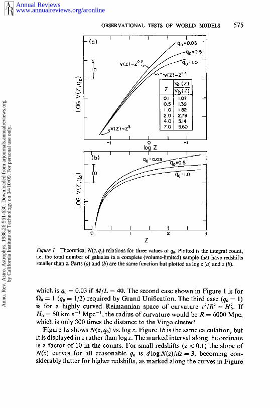
3.2 The Predicted N(z, qo) RelationCombining Equations 9-11 with Equations 29 and 30 gives the exactN(z, qo) relation, calculated therefrom directly in parametric form. A cal-culation via this route shows the dependence of N(z) on curvature forthree q0 values in Figure 1. The normalization of the volume is arbitraryin this diagram; N(z) is proportional to V(z), the proportionality factorbeing the volume density of galaxies,

The lowest value of q0 shown in Figure 1 is that which is required byadding the luminosity density of galaxies obtained from the observed N(m)data. As discussed by Binggeli et al. (1988) in their review of the luminosityfunction in this volume, this minimum permissible value of qo is

2q0 = 1.5 × IO-3(M/L), 31.


Ann

u. R

ev. A

stro

. Ast

roph

ys. 1

988.

26:5

61-6

30. D

ownl

oade

d fr

om a

rjou

rnal

s.an

nual

revi

ews.

org

by C

alif

orni

a In

stitu

te o

f T

echn

olog

y on

04/

10/0

9. F

or p

erso

nal u

se o

nly.



- (a)//qo=O.O$ -

/~..~qo=°’’5

-~o.v, z ,_ z~.~/./"~.~~’~.q.o- ,.o-

/// Vo

~0~ ~0 ~0

-I 0 ÷1log Z

I I I I I I _(b) qo=O~

(_9

0 I ~’

ZFigure 1 Theoretical N(z, qo) relations for three values of q0- Plotted is the integral count,i.e. the total number of galaxies in a complete (volume-limited) sample that have redshiftssmaller than z. Parts (a) and (b) are the same function but plotted as log z (a) and

which is q0 = 0.03 if M/L = 40. The second case shown in Figure 1 is forD.0 = 1 (q0 = 1/2) required by Grand Unification. The third case (q0 -- is for a highly curved Reimannian space of curvature c2/R2= H~. IfHo = 50 km s-1 Mpc-1, the radius of curvature would be R = 6000 Mpc,which is only 300 times the distance to the Virgo cluster!

Figure la shows N(z, qo) vs. log z. Figure lb is the same calculation, butit is displayed in z rather than log z. The marked interval along the ordinateis a factor of 10 in the counts. For small redshifts (z < 0.1) the slope N(z) curves for all reasonable q0 is dlogN(z)/dz = 3, becoming con-siderably flatter for higher redshifts, as marked along the curves in Figure


Ann

u. R

ev. A

stro

. Ast

roph

ys. 1

988.

26:5

61-6

30. D

ownl

oade

d fr

om a

rjou

rnal

s.an

nual

revi

ews.

org

by C

alif

orni

a In

stitu

te o

f T

echn

olog

y on

04/

10/0

9. F

or p

erso

nal u

se o

nly.


576 SANDAGE

la. For large redshifts, the volume becomes much smaller than the z3

Euclidean case for q0 > 1/2, but larger for the hyperbolic geometry ofqo < 0.5. The ratio of the volumes encompassed from the observer toredshift z for q0 = 0 compared with q0 = 0.5 is shown as a function ofz inthe table in Figure la.

4. THE REDSHIFT-MAGNITUDE EQUATION

4.1 The Predicted Hubble Diagram With No LuminosityEvolution

The N(z, q0) volume-redshift relation of the last section is very difficult apply in practice because complete galaxy counts in redshift space requireredshift measurements of every galaxy (of all types and surface brightness)in the volume, or else a correction for sample incompleteness in a redshiftsurvey that is complete to a given magnitude limit (Loh & Spillar 1986,Loh 1986). These corrections must be highly precise if the small differencesin the N(m, qo) curves in Figure 1 are to be measured. For this reason, thevalue of q0 via this route is quite uncertain at the moment.

The easier test observationally is the count-magnitude relation, N(m, qo),used in its most elementary form by Hubble (1936b), following the theoryset out by Hubble & Tolman (1935) for N(r). We now cast their discussioninto modern form by using the closed equation for the apparent mag-nitude-redshift relation via the Mattig equations and thereby changingN(z, qo) into the N(m, qo) count-magnitude prediction.

The apparent bolometric fluxf~ received at Earth from a galaxy recedingwith redshift z whose absolute flux (at the source) is Fb was shown Robertson (1938) (after some debate) to

Fb 32.f~ = 4n(R0r)2(1 +z)z"

For an appreciation of this equation, consider a sphere of interval radius1 (Equations 12, 13) centered on the source, over which the flux of a lightpulse is spread at the time of light reception, to, at the Earth. The area ofthis sphere is not 4nF if the geometry is non-Euclidean but is, rather,4n(R0r)~, where R0r = R0 sin l/R using Equation 12 for k = + 1. As in thecase of the spherical cap of Equation 5, this area is smaller than 4gl2 owingto the spatial curvature if k = + 1, or larger if k = - 1:

A(/) = 4rd 2 1- ~-~0~ +O ¯

The difference in the area compared with the Euclidean case is accounted


Ann

u. R

ev. A

stro

. Ast

roph

ys. 1

988.

26:5

61-6

30. D

ownl

oade

d fr

om a

rjou

rnal

s.an

nual

revi

ews.

org

by C

alif

orni

a In

stitu

te o

f T

echn

olog

y on

04/

10/0

9. F

or p

erso

nal u

se o

nly.


OBSERVATIONAL TEST8 OF WORLD MODELS 577

for in Equation 32 by the (Ror)2 factor rather than by simply using theinterval distance l, which would be incorrect. The (1 +z)2 term accountsfor the energy depletion and dilution factors of the radiation due to theredshift. One factor arises because each photon is decreased in energy by(1 +z), and hence the entire ensemble is depleted by the same factor. Thesecond factor of (1 +z) is present if the redshift is due to true expansion.It is caused by the increased path length, with the consequent decrease inthe energy density. If the Universe is not expanding, the second (1 +z)factor would not be present, a crucial point for the surface brightness testdiscussed in Section 8.

Converting Equation 32 into magnitudes and using Equation 30 for(R0r)2 gives the theoretical re(z, qo) equation for the Hubble diagram interms of the bolometric magnitude:

mbo~ = Mbo~+51ogq~2[zqo+(qo--1){--l+(2qoz+l)l/2}]+C, 33.

where the constant C is 2.5 log 4n + 5 log c/Ho. Note that the factor (1 + z)2

of Equation 32 is incorporated in Equation 33 as part of the theory. Someearlier writers, following Hubble, included the --5 log (1 ÷ z) factor as correction term to the observed magnitudes (as part of a generalized term). This is not the modern practice, however, which, as done here,carries this factor into Equation 33 via Equation 32. This point is veryimportant if the reader is to understand Hubble’s (1936b) method correction, which differs fundamentally from the modern practice, basedon the equations given here.

Series expansion of Equation 33 gives the well-known equation (e.g.Robertson 1955, McVittie 1956)

mboI = 5 log Z + 1.086(1 -- qO)Z + O(Z2) 34.

used by Humason et al. (1956; hereinafter HMS) in their early analysis cluster data. Although adequate to z ,-~ 0.3, the deviations of Equation 34from Equation 33 for larger z become inadequately large (cf. Mattig 1958,his Figure 1).

4.2 Conversion of Observed Heterochromatic Apparent

Magnitude to the Apparent Bolometric Scale:

The K Correction

The shift of the spectrum toward the red causes observed apparent mag-nitudes to differ from those that would have been observed at zero redshift.The correction is due to the fixed detector effective wavelength and thefinite detector bandwidth. As defined in current usage (HMS, appendix B;Oke & Sandage 1968), it is composed of two terms. The effective bandwidth


Ann

u. R

ev. A

stro

. Ast

roph

ys. 1

988.

26:5

61-6

30. D

ownl

oade

d fr

om a

rjou

rnal

s.an

nual

revi

ews.

org

by C

alif

orni

a In

stitu

te o

f T

echn

olog

y on

04/

10/0

9. F

or p

erso

nal u

se o

nly.


578 SANDAGE

in the rest frame of the source is smaller than in the rest frame of theobserver because the source spectrum is stretched upon redshift. Each rest-frame wavelength 20 appears to the observer at 20(1 +z), whereas thedetector bandwidth A20 is generally fixed. The bandwidth term due to thisstretching is 2.51og (l +z) magnitudes, in the sense that the correctedmagnitude must be brighter than the observed. The color-selective term isthe ratio of the flux of the redshifted spectrum to the unshifted spectrumthat is accepted by the detector. The term can be calculated by quadratureonce the rest-frame spectral energy distribution (SED) of the source known (the second term in Equation B7 of HMS).

Lack of accurate knowledge of the K correction was a stumbling blockin the early interpretations of (a) the galaxy counts (Hubble 1936b,Greenstein 1938), (b) the re(z) magnitude-redshift relation (Hubble 1953,HMS), and (c) the color evolution (Stebbins & Whitford 1948). Becauseof its crucial role in the interpretation of these cosmological test data, greateffort was made from 1960 to 1975 to measure the SED of galaxies ofvarious Hubble types. Early emphasis was put on E and SO galaxiesbecause of their dominance as first-ranked cluster galaxies. However, forthe galaxy count problem in the field, K(z) values for spirals of all Hubbleclasses (Sa, Sb, Sc, Sd, Sm, Im) are also required, together with knowledgeof the fractional morphological-mix of the sample.

Following Stebbins & Whitford~s (1948) early six-color broadbandmeasurements that gave highly smoothed 1(2) distributions (see also Whit-ford 1954), Code (1959) and Oke & Sandage (1968) obtained spectrumscanner data at 50 and 25/~ resolution of bright E galaxies. A study usingintermediate-band photometry was also made by Lasker (1970). Thesegave the first modern K corrections during the 1970s, although the datareferred only to the central ~ 15-arcsec regions of E galaxies in the Leoand Virgo clusters. Because the centers of E and SO galaxies are redder thanthe outer regions (de Vaucouleurs 1960, Tifft 1963, 1969, de Vaucouleurs de Vaucouleurs 1972, Sandage & Visvanathan 1978), these nuclear K(z)values were too large by progressive factors that reach ~ 0.1 mag at z -~ 0.3(Whitford 1971, his Figure 2). Schild & Oke (1971) and Whitford (1971)then used very large aperture photometry to account for the color gradient.From their integrated SEDs they calculated K(z) values in the B, V, andR photometric bands to redshifts of z = 0.28 for B and of z = 0.60 for Vand R, but again only for E and SO galaxies. Oke (1971~ then obtainedspectral scans of three distant (at that time) first-ranked cluster galaxiesat redshifts of z = 0.2, z = 0.38, and z -~ 0.46, giving usable SEDs for Egalaxies to 20 = 2700 /~ in the rest frame. This permitted K(B) to becalculated to z = 0.52 and K(V) and K(R) to z = 0.72 on the assumptionof no color evolution.


Ann

u. R

ev. A

stro

. Ast

roph

ys. 1

988.

26:5

61-6

30. D

ownl

oade

d fr

om a

rjou

rnal

s.an

nual

revi

ews.

org

by C

alif

orni

a In

stitu

te o

f T

echn

olog

y on

04/

10/0

9. F

or p

erso

nal u

se o

nly.



Wells (1972) measured I(2) from 3500 to 5500 ,~ for a range of galaxytypes. Using these data, to which OAO-2 data (Code et al. 1972) wereadded in the near-UV, Pence (1976) calculated K corrections for all galaxytypes to large redshifts, giving very useful comprehensive tables. FurtherUV data were added by Ellis et al. (1977). Using the final reduced datafrom the OAO-2, Code & Welch (1979) calculated new K corrections redshifts ofz = 1. Using these data, together with new observations madewith the ANS satellite, Coleman et al. 0980) calculated 1(2) energy dis-tributions for old stellar populations and for Sbc, Sod, and Im galaxies to20 = 1400 ,~ and gave comprehensive Kcorrections in the U, B, ~’, and Rphotometric bands to z -- 2. These data are the most extensive K cor-rections now available in the standard broadband photometric system,providing an enormous advance in this crucial problem since the earlyanalysis by HMS. Sebok (1986), using the energy distributions of Wells,listed K(z) for all morphological types for the Thuan-Gunn red system.Schneider et al. (1983a) list K(z) for the Thuan-Gunn g, r, i~ and z bandsfor giant E and SO galaxies.

A summary of the SEDs in the archive literature that have been used tocalculate K and the color variations with z is given by Yoshii & Takahara(1988) in their valuable review of cosmological tests.

4.3 The Predicted Hubble Dia#ram With Correctionfor Luminosity Evolution

In an evolving universe, the mean age of galaxies decreases with increasingredshift simply because we sample earlier times as we look out in distance.A first estimate of the expected change of E galaxy luminosities with look-back time, based on the change of the turnoffluminosity in the HR diagramfor an old coeval population, gave a mean evolutionary rate of L ~ t-4/3

for a flat luminosity function at the main sequence turnoff (Sandage1961b). Because the luminosity function is not flat but rises for faintmagnitudes below the turnoff, this is an upper limit, overestimating theluminosity rate by about 30%.

Call the change of magnitude due to evolution E(t)~ Equation 33, trans-formed to heterochromatic magnitudes, then becomes

m~ = M~--K~(z)--E~(t)+ 51ogq~2

x [zqo+(qo-- 1) {-- 1 +(2q0z+ 1)~/2}]+C,

which is a basic equation that is used extensively in the following sections.As for the size of E(t), the simple evolution rate for an old coeval

population of L ~ t -4/~ quoted above would give a magnitude variationof A mag = --2.5 log to/t~, where to and t~ are the ages of the source at light


Ann

u. R

ev. A

stro

. Ast

roph

ys. 1

988.

26:5

61-6

30. D

ownl

oade

d fr

om a

rjou

rnal

s.an

nual

revi

ews.

org

by C

alif

orni

a In

stitu

te o

f T

echn

olog

y on

04/

10/0

9. F

or p

erso

nal u

se o

nly.


580 SANDAGE

reception at the Earth and at light emission from the source, respectively.If t0 = 15 x 109 yr and we inquire for the case of a look-back time of 109

yr, then A mag = --2.5 log (15/14)4/3 = 0.10 mag for small toil. The senseof the correction is that galaxies were brighter in the past. If this rate is~ 30% too high (Tinsley & Gunn 1976), the rough estimate of E(t) is ~0.07 mag per 109 yr.

Elaborate calculations of E(t) form the subject of galaxy evolution viastellar population synthesis, pioneered by Tinsley (1968, 1972a,b, 1976,1977a,b, 1980, and references therein) and her colleagues. The exact ratedepends on the various assumptions of star formation rates over time andon the slope of the main sequence luminosity function. However, order-of-magnitude corrections, changing t to z via equations in the next section,give Am ~ -2.5 log (1 d-z). For small z the correction again is approxi-mately 0.07 mag per l0 9 yr on a time scale of to "~ 15 x 109 yr for the ageof the Universe--nearly the same as the early, quite elementary estimates.

For very large redshifts, where the look-back times are of the order ofthe age of the Universe, much more elaborate evolutionary models arerequired than simple main sequence burn-down rates near the presentmain sequence termination point. The philosophy by which the rates canbe calculated near the beginning of galaxy formation was first set out byTinsley (1968). Modern calculations include those of Bruzual & Kron(1980), Bruzual 0981, 1983a,b), and Arimoto & Yosh~i 0986, 1987). summary of E(t) over the age range of l07 to 1.5 × l0~° yr is given byYoshii & Takahara 0988, their Figure 2) for E/S0 and Sdm galaxies inthe UBVRIJK photometric bands.

4.4 The Look-Back Time as a Function of.4 and qo

To use Equation 35 we must change E(t) into E(z) by the relation betweenthe look-back time z = t0-tl and the redshift as a function of q0. Thegeneral case requires the closed solution of R(t) from the Friedmannequation. Before setting down this general solution, it is instructive toconsider again the simple cases of q0 -- 0 and q0 -- 1/2 for empty space andfor flat space-time, respectively.

Recall that R(t) ,,~ for q0= 0and R(t)t2/3 for q0 = 1/2. Using thesedependencies and the Lemaitre equation of Ro/RI = 1 ~-z gives the fol-lowing relations for the look-back time:

¯ =-~H;-~ 1 for q.-- 1/2. 37.


Ann

u. R

ev. A

stro

. Ast

roph

ys. 1

988.

26:5

61-6

30. D

ownl

oade

d fr

om a

rjou

rnal

s.an

nual

revi

ews.

org

by C

alif

orni

a In

stitu

te o

f T

echn

olog

y on

04/

10/0

9. F

or p

erso

nal u

se o

nly.



The general case for any q0 is found by combining the age equations(Sandage 1961a, Equations 61 and 65) of To=f(qo, Ho) with theRo/Rl = q(z, qo) Friedmann solution, together with Ro/R~ -- 1 + z. Tablesare given in Sandage (1961b).

5. PREDICTED AND OBSERVED COUNT-

MAGNITUDE RELATION

5.1 Method of Predicting N(m, qo, E) for an InfinitelyNarrow Luminosity Function

The necessary apparatus is now in place to predict the expected N(m)relation for any assumed q0 value and luminosity evolution rate E(z). TheN(z) relation calculated by the method of Section 3.2 can be transformedto N(m, qo, E) using Equation 35. The conversion is trivial if M is assumedto be a fixed number, (M), with no dispersion (i.e. if the luminosityfunction is a spike). In this case, for computational purposes the equationsare easiest used progressively in parametric form with the following steps,once q0 has been fixed for a particular geometry.

1. For any particular redshift z, calculate r and rRo from Equations 29and 30.

2, Use Equations 9, 10, or 11 (depending on the value of k) to calculateV(z), which aside from a normalization factor is the N(z, qo) of Section3.2.

3. For any z and q0 use Equation 35 to calculate m for an assumed absolutemagnitude (M), using the K(z) and E(z) corrections.

4. Repeat for a variety of z and q0 values, producing the predicted familyof N(m, qo) curves.

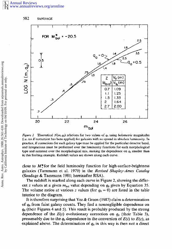
These steps are the method that was used to show numerically thedegeneracy of N(m) to q0 to first order in z (Sandage 1961 a, his Figures and 5) if E(z) = 0, despite the nondegeneracy to q0 in N(z). The sameresult that N(m) is less sensitive to q0 than is N(z) was shown analyticallyby Robertson & Noonan (1968), Misner et al. (1973), and Brown & Tinsley(1974) using series expansions. The reason for the near-degeneracy of theN(m) counts to q0 is that although the N(z) relation is relatively sensitiveto q0, its dependence on q0 appears with the opposite sign from the variationof m(z) with q0 in Equation 35. This nearly cancels the curvature depen-dence of N(m, qo). The calculated N(m, qo) curves with no K correction(i.e. using the m~o~ magnitude scale) are shown in Figure 2 for q0 = 0 andqo = 0.5. For this idealized calculation, all galaxies were assumed to havethe same absolute magnitude of gbot ----- --20.5; this is a reasonable value,


Ann

u. R

ev. A

stro

. Ast

roph

ys. 1

988.

26:5

61-6

30. D

ownl

oade

d fr

om a

rjou

rnal

s.an

nual

revi

ews.

org

by C

alif

orni

a In

stitu

te o

f T

echn

olog

y on

04/

10/0

9. F

or p

erso

nal u

se o

nly.


582 SANDAGE

i I I i I I I [

FOR M=v~,,I = - 20.52.5

-- -- ,,., 1.4 J~.5 --

~.5 =

.1,5 L33.52 1.64~ 2.7 2.oo

.2

I I I I I I I I ,20 22 24 26

m bol

Figure 2 ~eoretica[ N(m, qo) relations for two values of qo using bo[ometric ~a~itudes(i,¢.. ~o K ¢oE¢¢tio~ has been applied) for gala~es with ~o spread in absolute lu~nosity. prattle, Kcorr¢ctions for each galaxy type must be app~cd for the pa~i¢ular det~tor band,and int¢~atioBs m~st be perfo~ over the l~osity functions for eaCht~¢ and su~¢d over the mo~holo~l ~x, making the dependen~ on q0 smaller than

close to M~*for the field luminosity function for high-surface-brightnessgalaxies (Tammann et al. 1979) in the Revised Shapley-Ames Catalog(Sandage & Tammann 1981; hereinafter RSA).

The redshift is marked along each curve in Figure 2, showing the differ-ent z values at a given rnbo~ value depending on q0 given by Equation 35.The volume ratios at various z values (for q0 = 0) are listed in the tableinterior to the diagram.

It is therefore surprising that Yee & Green 0987) claim a determinationof q0 from faint galaxy counts. They find a nonnegligible dependence onq0 (their Figures 4 and 5). This result is probably produced by the strongdependence of the E(z) evolutionary correction on qo (their Table 3),presumably due to the q0 dependence in the conversion of E(t) to E(z), asexplained above. The determination of q0 in this way is then not a direct


Ann

u. R

ev. A

stro

. Ast

roph

ys. 1

988.

26:5

61-6

30. D

ownl

oade

d fr

om a

rjou

rnal

s.an

nual

revi

ews.

org

by C

alif

orni

a In

stitu

te o

f T

echn

olog

y on

04/

10/0

9. F

or p

erso

nal u

se o

nly.



test of different volumes of a non-Euclidean geometry (i.e. the direct volumetest) but rather a much more indirect route that connects secular luminosityevolution with a time scale that does depend on H0 and q0 (Section 9).

5.2 The Full Complication of the N(m, qo, E) Prediction,Given E(z) and the Luminosity Function gO (M,

For the real case we must integrate over the luminosity function. Becausethis function changes in shape and normalization with galaxy type (Bing-geli 1987, Binggeli et al. 1988) and because K(z) in Equation 35 is also astrong function of type, separate integrations are required for each Hubblemorphological class. The results for a given type are then summed overall types using an assumed galaxy mix.

The integration over absolute luminosity, and over the sheets and voidsof the galaxy distribution, is done by the usual equation of stellar statistics:

A(m, T) = C ~ D(z, T)dp(M, T) dr(z, qo), 38.

where A(m, T) is the number of galaxies of type T per unit area at m ininterval dm, C is a normalization factor used to convert the absolutedensity (in number of galaxies of type T per cubic parsec) to units number of galaxies per unit area, D(z, T) is the density at distance z oftype T, ~b(M, T) is the luminosity function read at M in interval dM forgalaxies of type T, and dV(z, qo) is the volume element between redshiftz~ and z2 corresponding to the magnitude interval between m-dm andrn + dm.

The total number of galaxies brighter than m is

N(m, qo)=frffA(m,T)dTdm, 39.

i.e. A (m, T) summed over type and magnitude.To apply Equation 38 we must use Equations 9-11, 29, and 30 for

V(z, qo), together with the m(M, z, qo, E) relation of Equation 35. In thisway, all variables in Equation 38 can be related to each other, albeit in amultiparametric way.

The simplest practical method for solving Equation 38 is to replace theintegral by a summation over shells bounded by redshifts zl and z2, suchthat the apparent magnitude [for fixed M- K(z) -- E(z) values] at z2 differsby one magnitude from that at zl. An m, log g-like table can then beconstructed by the method of Kapteyn (cf. Bok 1931, 1937, Mihalas Binney 1981). Such a table has cells separated by a unit apparent mag-nitude interval along the top of each column and by z~ and z2 boundaries


Ann

u. R

ev. A

stro

. Ast

roph

ys. 1

988.

26:5

61-6

30. D

ownl

oade

d fr

om a

rjou

rnal

s.an

nual

revi

ews.

org

by C

alif

orni

a In

stitu

te o

f T

echn

olog

y on

04/

10/0

9. F

or p

erso

nal u

se o

nly.


584 SANDAGE

for the rows. In each (m, Zl-z2) cell a particular M-K(z)-E(z) applies via Equation 35. The volume element in each row, given by Equa-tions 9-1 l, 29, and 30, can be multiplied by the (M, T) and D(z) applies to each cell [i.e. at a given (z) = 1/2(z~+z2)]. The sum of column is the A(rn) value for a given type. The process is then repeatedfor each type, and the A(m) values are summed via Equation 38 to giveN(m, qo).

This, or an equivalent method, has presumably been used by thosewho compare galaxy counts with predictions of the models, although themethods have not been described in detail in any of the original archivepapers in the literature, now to be discussed.

5.3 Observations

5.3.1 RESULTS BEFORE ~ 1970 Galaxy counts were used near the beginningof this century to study the surface distribution of nebulae in efforts toestablish their nature. Seares’ (1925) definitive paper (a) established latitude dependence, (b) emphasized the zone of avoidance, and (c) redis-covered the north Galactic pole anomaly [following Humboldt (1866)(quoted by Zwicky 1957)], a feature now called the Local Supercluster (deVaucouleurs 1956). Scares’ work, following that of Proctor (1869), Hinks(1911), Fath (1914), Hardcastle (1914), and Reynolds (1920, 1923a,b),struck at the heart of these surface distribution problems, solving them inprinciple and preceding Hubble’s (1931, 1934) massive study with itsstraightforward definitive presentation.

Shortly after his discovery of Cepheids in M31 and NGC 6822 (Hubble1925a,b), Hubble (1926) wrote his central paper on the general propertiesof galaxies. As part of the discussion, he analyzed galaxy number countsover the magnitude range mpg = 8.5-16.7 from various earlier sources.These data provided the first reliable N(m) relation, showing thatlogN(m) = 0.6m+constant. The coefficient for m was 0.6 to within theerror, showing beyond doubt (and for the first time) that nebulae aredistributed homogeneously in the lar~te (i.e. when averaged over an appreci-able solid angle). The same conclusion was reached by Shapley & Ames(1932, their Figure 6) from counts brighter than mpg = 13. The slopecoefficient of log N(m) is 0.6 for any homogeneously distributed luminoussources, no matter what their luminosity distribution, provided only thatthe geometry is at least approximately Euclidean (vonder Pahlen 1937,Bok 1937).

Hubble’s demonstration that log N(m) varies as 0.6m was a crucial proofthat galaxies provide a fair sample with which to study the large-scalematter distribution of the Universe. Galaxies are not merely a localphenomenon as part of a larger hierarchy. To be sure, larger structures of


Ann

u. R

ev. A

stro

. Ast

roph

ys. 1

988.

26:5

61-6

30. D

ownl

oade

d fr

om a

rjou

rnal

s.an

nual

revi

ews.

org

by C

alif

orni

a In

stitu

te o

f T

echn

olog

y on

04/

10/0

9. F

or p

erso

nal u

se o

nly.



clusters of galaxies and clusters of clusters do exist. Shapley (1932), Bok(1934), and Hubble (1934, his Figure 7) did discuss the clustering tendency.Nevertheless, grand averages at various distances, taken over large-enoughsolid angles, show no sign of progressive diminution from homogeneity(Sandage et al. 1972) as would be present ins Charlier-like hierarchy [butsee de Vaucouleurs (1970) for an opposite opinion].

Galaxy counts to magnitudes fainter than 16.7 were made by Hubble(1934), Mayall (1934), and again by Hubble (1936b), giving five additionalpoints for N(m) at m -- 18.1, 18.8, 19.1, 20.0, and 21.0 on the magnitudescale extant in 1936.

Analyzing these data, Hubbl¢ (1936b, 1937) concluded that the spatialcurvature had been robustly detected. But its radius of curvature was sosmall, if the magnitude correction terms due to redshift were correct, tocause him to question if the redshift was due to a true expansion. Hisanalysis followed the formalism developed by Hubble & Tolman (1935),applying the K(z) correction and also the (1 + z) ~ term of Equation 32 tothe data. Hubble stated that the unbelievably small radius of curvaturecould be avoided if only one factor of (1 +z) were to be used rather thantwo, from which it would follow that the number effect in the path-lengthdilution of the photons would not occur, meaning no expansion.

This astonishing conclusion would not be reached today even using thesame observational N(m) data, i.e. even if it were assumed that the 1934apparent magnitude scale was correct. First, Hubble’s K(z) correction wasbased on a blackbody spectrum of temperature 6000 K, whereas the realenergy distribution is not a blackbody, and further the color temperatureis much smaller (Greenstein 1938). In addition, Hubble mistakenly hadno bandwidth term [2.5 log (1 +z)] in his K(z) correction. Second, Figure2 shows that the correct m(z) equation put into the V(z) relations givesmuch too small a dependence of N(m) on q0 to measure the space curvaturein this way. Although an adequate comparison of Hubble’s (1936b) analy-sis with the modern theory of the standard model has not yet appeared,it is believed that even the sign of his correction term to remove theuncomfortably small radius of curvature is opposite to what we wouldapply today. A rediscussion of Hubble’s analysis in modern terms wouldbe of considerable historical interest.

5.3.2 RECENT GALAXY COUNT DATA AND ANALYSIS The extensive LickSurvey by Shane & Wirtanen (1950, 1967, and prior references), sum-marized by Shane (1975), began the modern work on the surface galaxydistribution. This survey added a point at mpg = 19.0 to the N(m) data,but most importantly it began to show the true fine structure of the surfacedistribution. The first striking evidence for filaments (anticipated, to be


Ann

u. R

ev. A

stro

. Ast

roph

ys. 1

988.

26:5

61-6

30. D

ownl

oade

d fr

om a

rjou

rnal

s.an

nual

revi

ews.

org

by C

alif

orni

a In

stitu

te o

f T

echn

olog

y on

04/

10/0

9. F

or p

erso

nal u

se o

nly.


586 SANDAGE

sure, by Shapley’s extensive Bruce telescope survey to 17 mag discussed inmany issues of the Harvard Circulars and Bulletins in the 1930s and 1960s)was found by Seldner et al. (1977, Plate I). This was the beginning of thecurrent emphasis on sheets and voids in the three-dimensional spatialgalaxy distribution, discovered by Tifft & Gregory (1976), Chincarini Rood (1976), and especially Gregory & Thompson (1978, their Figure These early results are reviewed in these volumes by Oort (1983).

The existence of the sheets and voids (cf. Kirshner et al. 1981, Haynes& Giovanelli 1986, de Lapparent et al. 1986) calls into question the veryvalidity of the count-volume test for measuring the spatial curvature. Onthe scale of 100 Mpc, the distribution of galaxies is clearly not homo-geneous in detail. However, it is precisely the necessity of this exact detailthat is important if the slight deviations of V(z) from Euclidean volumescan, even in principle, be found.

The existence of local inhomogeneities at all redshifts is demonstratedby pencil-beam surveys of redshift distributions, i.e. the number of galaxies¯ in a complete sample at redshift z in dz in the magnitude interval dm at m.The theoretical expectation of this distribution is predicted directly by theappropriate sums in the m, log r~ table solutions of Equation 38, asdescribed in Section 5.2 and by Binggeli et al. (1988, Section 1.2.2) in thisvolume. Preliminary observational data from two independent pencil-beam redshift studies by Ellis (1987, his Figure 6) and by Koo & Kron(1987, their Figure 1), although clearly showing the voids, have upper-envelope distributions N(z) that are well defined for each data set. Thismight be used to justify a belief that if averages are taken over sufficientlylarge areas, the small-scale sheet and void fluctuation distribution willcancel out exactly, leaving only a spatial curvature signal. This optimisticview keeps alive the hope for a geometrical solution to the Gauss-Schwarz-schild experimental methods to find kc~/R2 that we have been discussing.Yet it seems that this approach, in view of the very great inhomogeneitieson 100-Mpc scales, is looking more and more like an optimistic climb tothe summit of Everest without proper equipment. Yet to remain in thevalley is to miss the chance to view the ineffable scene from the summit,on the off chance of reaching it.

In this spirit, first results of many deep-count surveys are now in theliterature. Ellis (1987) has reviewed the counts in the (near) B photometricband determined by seven research groups. Differences in the absolutevalue of N(m) between these various independent surveys exist at the levelof a factor of about 2 at m -~ 21 and fainter. It is not yet known if this isdue to differences (errors) in the magnitude scales used by the variousobservers or to real differences between the regions surveyed. To date, the


Ann

u. R

ev. A

stro

. Ast

roph

ys. 1

988.

26:5

61-6

30. D

ownl

oade

d fr

om a

rjou

rnal

s.an

nual

revi

ews.

org

by C

alif

orni

a In

stitu

te o

f T

echn

olog

y on

04/

10/0

9. F

or p

erso

nal u

se o

nly.



areas in each survey have necessarily been very small owing to the enor-mous problem of data reduction of charge-coupled device (CCD) framesbetween B ~ 23 and 26.

On the assumption that the grand average will produce an adequateapproximation to homogeneity, so that the data can be compared with theN(m, qo, E) predictions of the last section, Yoshii & Takahara (1988, theirFigure 8) combined the seven surveys [Jarvis & Tyson (1981), Shanks al (1984), Peterson et al. (1979), Kirshner et al. (1979), Kron (1980a,b),to which can be added Ciardullo (1986), as in Ellis (1987, his Figure and Yce & Green (1987)]. Their diagram showing the differential A(m)counts is reproduced here as Figure 3. Superimposed are the theoreticalA(m, qo, E) curves as calculated by Yoshii & Takahara by a method’ onlybriefly explained, but one that appears to be equivalent to what we havegiven in the last section. In their calculations they used the luminosityevolution function E(t) (their Figure 2) derived by Arimoto & Yoshii(1986, 1987), together with a galaxy morphological r~ix by Tinsley (I 980),similar to that adopted by Pence (1976) and by Ellis (1983).

The most important and best-established result of the major surveys todate is that each data sample shows that dlog N(m)/dm = 0.6 for B brighterthan 16. This was also shown in detail by Sandage et al. (1972), whosummarized earlier data in regions far from the north Galactic anomaly,confirming Hubble and Mayall’s (Hubble 1934, 1936b, Mayall 1934) priorcentral result obtained in the mid-1930s, mentioned earlier. Also highlysatisfactory is the observed decrease of the slope for B > 18, reachingdlogA(m)/dm 0.4 atB =20, which is t he predicted valu e as shown bythe theoretical lines in Figure 3. Except for the faint AAT points, whichshow a factor of 2 excess over the other surveys, the counts and the theoryagree moderately well using q0 ~ 0.02 and a galaxy formation redshift ofzr ~ 5. This conclusion is the same as that which can be made from Figure2 of Ellis (1987), where the no-luminosity evolution line lies far below theobservations, showing that appreciable luminosity evolution is requiredeven at z ~ 0.4 to fit the faint count data. The conclusion for luminosityevolution depends, however, on the explicit assumption that the standardmodel is correct.

It is important to emphasize that no check on the direct predictions ofthe standard model is available from this test, or indeed from any of thefollowing tests (except for that of the time scale; see Section 9), unless priori assumptions are made concerning .the evolution. It is this aspect ofobservational cosmology that is so fragile and that poses the most seriousquestions at the moment concerning the efficacy of the standard tests--with the sole exceptions of (a) the time-scale test, (b) the several inde-


Ann

u. R

ev. A

stro

. Ast

roph

ys. 1

988.

26:5

61-6

30. D

ownl

oade

d fr

om a

rjou

rnal

s.an

nual

revi

ews.

org

by C

alif

orni

a In

stitu

te o

f T

echn

olog

y on

04/

10/0

9. F

or p

erso

nal u

se o

nly.

iOs

104

IO¯ Jorvis ~ Tyson (1981),) UKST

/ ShonP.s et ol. (1984)AATUKST I"

~ Peferson ef o1.(1976)

~, OARS+ KOS

I I I I I I, I I ! ,,t 4 t 6 18 2Q 2.2 24 ~6 28 :50

8~ (mog)

Figure 3 Comparison of predicted A(m, qo) functions with the observed differential counts(i.e. number at magnitude Bj in magnitude interval --+0.25 mag) from various surveys. Thefour heavy lines to the left are for the marked values of q0 and the redshift of galaxyformation, with luminosity evolution included. The four light lines to the right are the samebut with zero luminosity evolution. The relations depend on Ho only to set the time scale forthe galaxy luminosity evolution correction (from Yoshii & Takahara 1988).


Ann

u. R

ev. A

stro

. Ast

roph

ys. 1

988.

26:5

61-6

30. D

ownl

oade

d fr

om a

rjou

rnal

s.an

nual

revi

ews.

org

by C

alif

orni

a In

stitu

te o

f T

echn

olog

y on

04/

10/0

9. F

or p

erso

nal u

se o

nly.



pendent predictions and later discovery of the 3-K Gamow, Alpher, andHerman radiation, and (c) the predictions of nucleosynthesis in the veryearly phases of the standard model (Boesgaard & Steigrnan 1985).

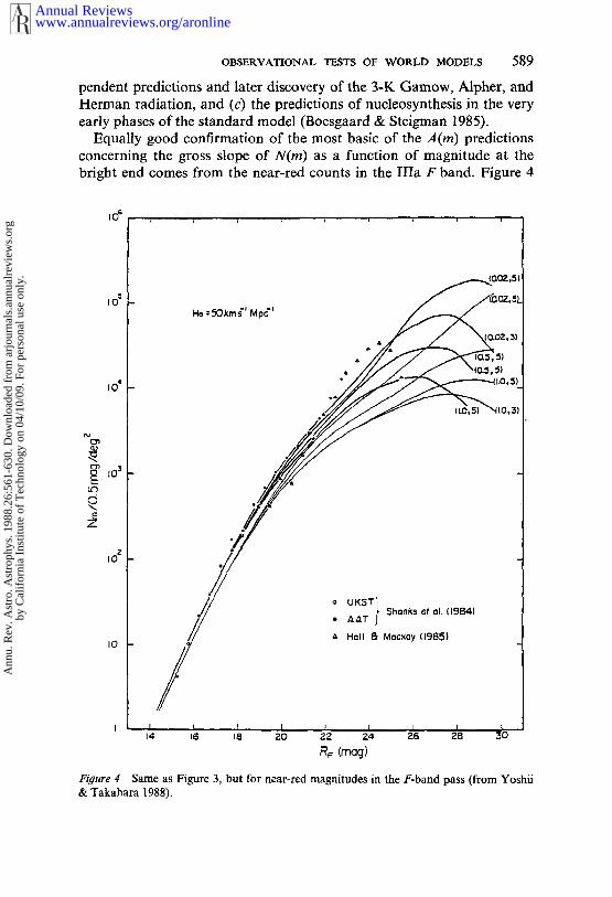
Equally good confirmation of the most basic of the A(m) predictionsconcerning the gross slope of N(m) as a function of magnitude at thebright end comes from the near-red counts in the IIIa F band. Figure 4

I0

Fi#ure 4

UKST~’i Shanks ¢t ol. 11984]

Hall 8i Mackay 11985)

~ 4 ~6 ~ 8 20 22 24 26 28

Same as Figure 3, but for near-red magnitudes in the F-band pass (from Yoshii

& Takahara 1988).


Ann

u. R

ev. A

stro

. Ast

roph

ys. 1

988.

26:5

61-6

30. D

ownl

oade

d fr

om a

rjou

rnal

s.an

nual

revi

ews.

org

by C

alif

orni

a In

stitu

te o

f T

echn

olog

y on

04/

10/0

9. F

or p

erso

nal u

se o

nly.


590 SANDAGE

(taken from Figure 9 of Yoshii & Takahara 1988) shows the comparisonbetween observations and the model. The data are from Shanks et al.(1984) and Hall & Mackay (1984).

Aside from the gross agreement of slopes, Figures 3 and 4 show againthe chief result expected earlier (Brown & Tinsley 1974) that the/l(m, qo, E)differential test, or the N(m, q0, E) integral test, has little hope of findingq0 because of (a) the first-order insensitivity to the curvature, and (b) lack of detailed homogeneity due to the sheet and void properties of thedistribution, making the test probably impossible even in principle.

The m(z) test (i.e. the Hubble diagram) entirely avoids this latter prob-lem as long as the inhomogeneifies do not induce large velocity per-turbations on the Hubble flow at high z, which they certainly do not. Theupper limit to such perturbations is of the order ,~ 500 km s- 1 given bythe noncosmological motion of the Local Sul~rcluster relative to themicrowave background [see Tammann & Sandage (1985) for a review];this is a subject for which a large literature now exists (cf. Dressler et al.1987). Such perturbations at redshifts z ~ 0.5 give velocity perturbationsAv/v ,~ 0.0003, which have negligible effect on re(z), as we now show.

6. THE m(z) HUBBLE DIAGRAM

6.1 Local Tests for Linearity of the Redshift-

Distance Relation

6.1.1 ~ PREDICTIO~q If redshift is due to a real expansion of thegeometrical manifold carrying the galaxies with it, the form of the velocityfield must be isotropic and linear if space is isotropic and homogeneous.There are many ways to prove this. One of the most straightforward is toconsider a triangle. If, upon expansion, the triangle is to be similar to itself,it follows directly that the velocity vi of any number of points along thesides of the triangle at distances ri from any arbitrary point must be

Vi = H(t)ri. 40.

Otherwise the sides of the triangle will not expand with the same propor-tionality ratio. The factor H(t) sets the scale of the velocity field at time t.

A linear velocity field has two fundamental properties:

1. The form and the scale of the field are invariant to position, i.e. Equation40 holds for every point in the manifold upon transferring the originto it. Hence, the velocity field looks the same from every vantage point,i.e. the ultimate democracy.

2. Upon reversing direction of the velocity vectors to form a contractingfield, all points arrive at the origin at the same time, i.e~ points twice as


Ann

u. R

ev. A

stro

. Ast

roph

ys. 1

988.

26:5

61-6

30. D

ownl

oade

d fr

om a

rjou

rnal

s.an

nual

revi

ews.

org

by C

alif

orni

a In

stitu

te o

f T

echn

olog

y on

04/

10/0

9. F

or p

erso

nal u

se o

nly.



far away as others have twice the velocity, hence equal travel time toany arbitrary point. And because all points are equivalent, all pointsarrive at all other points together. There is no center of the expansion.All points have always been the center.

From these two properties it was early expected that the velocity-dis-tance relation for any reasonable model of an isotropic, homogeneousuniverse (in the large) must be linear if redshift is a true expansion of themanifold. Note also that the direct prediction of the m(2) relation in thestandard model (Equations 33 and 34), using m-M+5 = 5log r, givescz = Hor in the z-~ 0 limit, which is Equation 40; this provides anotherway to prove that linearity is a prediction of the standard model.

6.1.2 THE DATA FOR SMALL z For light travel times that are smallcompared with the age of the Universe, the World picture is nearly thesame as the World map, in Milne’s (1935) useful language. The light traveltime can be neglected for small-enough redshifts.

In the search for the fo~m of the expansion law, the relevant redshiftregime in which to exploit this circumstance unencumbered by the non-simultaneity of the observations is z _< 0.2.

Four claims are extant in the literature concerning the dependence ofredshifts on distance in the World map. Only one of the following iscorrect.

1. The relation is linear everywhere, at all distances and at all times. Thestandard model requires it. We argue herein that the data demand it.

2. The relation is approximately quadratic locally (i.e. to cz ~ 4000 kms-l); thereafter it becomes linear (de Vaucouleurs 1958, 1972, de Vau-couleurs & Peters 1986, their Figures 2a,b; Giraud 1985, 1986a,b, 1987).

3. The relation is quadratic everywhere (Segal 1975, 1981).4. The relation is exponential as 1 + z = exp (HrR/c) in the speculation of

tired light [LaViolette 1986; see also Pecker & Vigier (1987) for review].

In his discovery paper, Hubble (1929) claimed a linear relation onlyquite locally, being aware of de Sitter’s (1917) quadratic prediction [cf.Sandage (1975b) for a history]. Hubble’s final sentence of this first paperwas a cautious "and in this connection it may be emphasized that thelinear relation found in the present discussion is a first approximationrepresenting a restricted range in distance." His idea evidently was that hemight only be observing a linear (tangent) approximation at very small to the de Sitter v ~ r~ prediction, which might become evident at larger

¯ distances.To test this, Humason (1931) began redshift rneasurements at Mount


Ann

u. R

ev. A

stro

. Ast

roph

ys. 1

988.

26:5

61-6

30. D

ownl

oade

d fr

om a

rjou

rnal

s.an

nual

revi

ews.

org

by C

alif

orni

a In

stitu

te o

f T

echn

olog

y on

04/

10/0

9. F

or p

erso

nal u

se o

nly.


592 SANDAGE

Wilson of bright E galaxies in clusters and found, even at this early date,values as large as cz ,~ 20,000 km s-i for a cluster in Leo. With thesenew data, combined with estimates of apparent magnitude, Hubble &Humason (1931) extended the original velocity-apparent magnituderelation approximately twentyfold in distance within two years of theinitial discovery.

The slope of the redshift-magnitude relation was found to be 5 to withinthe errors, proving beyond doubt that the velocity-distance law is linear.However, in 1931 there were only 8 dusters involved in the test. By 1936,Hubble (1936a) and Humason (1936) had increased the data base to dusters reaching cz = 42,000 km s- ~, with the same result. Hubble’s (1953)last discussion, in his Darwin lecture, still had only 11 clusters, but thedata now reached to z = 0.2, which was the largest redshift Humasoncould measure, even with the early use of the Palomar 200-inch reflectorwith photographic detection. The result again proved linearity, but thedata sample was still small and the photometric measurements had beenmade using only photographic techniques. The final phase of the initialproof of linearity was the summary paper of HMS, which used new dataon 18 clusters. However, the universality of the phenomenon was moreinferred than established because there were still so few clusters.

Early claims of nonlinearity (cf. Hawkins 1962) used the HMS data field galaxies taken from flux-limited samples and failed to correct forsample bias. Modern discussions of local nonlinearity, some of whichare referenced earlier in this section, also use field galaxies. Because theluminosity function of field galaxies is considerably broader than for first-ranked cluster galaxies, some conclusions from these field galaxy studieshave been criticized as due to insufficient corrections for the selection bias.Discussions of the bias have been given by Teerikorpi (1975a,b, 1984,1987), Bottinelli et al. (1986, 1987, 1988), and Sandage (1988a,b). principal consequences of bias neglect have been (a) an incorrectly highvalue of the Hubble constant and (b) a false belief that the consequentcalculated variation of H0 with distance, increasing outward, is real (Sec-tion 9).

Discussion of the bias effects in the flux-limited RSA catalog becamepossible when the redshift coverage of that catalog became complete,following the finalization (Sandage 1978) of the Humason & Mayall(HMS) redshift program. The bias in the field galaxy sample was showndirectly (Sandage et al. 1979), and the apparent increase of H0 with distancewas demonstrated to be an artifact, caused by assigning a fixed (M) valueto all galaxies in the flux-limited sample. These selection effects are severeenough that study of the form of the redshift-distance relation using fieldgalaxies is dangerous owing to the necessary corrections that are difficult


Ann

u. R

ev. A

stro

. Ast

roph

ys. 1

988.

26:5

61-6

30. D

ownl

oade

d fr

om a

rjou

rnal

s.an

nual

revi

ews.

org

by C

alif

orni

a In

stitu

te o

f T

echn

olog

y on

04/

10/0

9. F

or p

erso

nal u

se o

nly.



to make accurately. For this reason, study of the re(z) relation to test forlinearity was begun in the early 1970s using cluster and group samples.The photometry in these studies was done by photoelectric techniques; theresults, reported in a series of papers (Sandage 1972a,b,c, 1973a,b, 1975a,1986, Sandage et al. 1972, Sandage & Hardy 1973), again confirmed thelinearity of the local velocity-distance relation.

The principal conclusion of the work was that the leading term of5 log cz in the theoretical prediction of Equation 34 is fully confirmed. Thestandard model does, then, pass this most elementary of its predictions.

6.2 The Hubble Diagram at Large Redshifts

Determination of the second term involving q0 in Equations 33-35 was theprincipal motivation for extending the Hubbl¢ rn(z) diagram to the largestpossible redshifts. The correction is of first order in z (cf. Equation 34)and hence is a large effect. To see how large, recall the special cases of

q0 = 0 and q0 = 1/2 for Rro of Equations 22 and 26, which (when put intoEquation 32 for the flux) give the closed expressions

mbo~=51og 2 1+ +constant for qo=0, 41.

and

mbo~ = 51og[2(l+z--x//~+z)]+constant for q0 = 1/2, 42.

where the constant is the same in both equations. These are special casesof the general equation (Equation 33). If, then, we could observe to z = 1 anddetermine rnbo~, the magnitude difference between the q0 = 0 and q0 = 1/2cases would be Ambol = 0.54 mag, the qo = 1/2 case being brighter,assuming no luminosity evolution in the look-back time.

Early studies aimed to determine qo this way were reviewed by Peach(1970, 1972). Special programs to extend the Hubble diagram to verylarge redshifts were begun by Gunn & Oke (1975), Sandage et al. (1976),Kristian et al. (1978), Hoessel (1980), and Schneider et al. (1983a,b), these studies reached redshifts of z = 0.5 (excluding the radio galaxies).Very much larger redshifts for cluster galaxies have become available byincluding radio sources in the sample [see Spinrad (1986, and referencestherein) for a review].

6.2.1 COP.~CT~ONS TO TI4E MAGNITUDES FOR THE I-IUBBLE DIAGRAMSeveral technical corrections are needed before Equation 35 can be usedto obtain q0.

1. The aperture correction must b~ made to reduce the photometric


Ann

u. R

ev. A

stro

. Ast

roph

ys. 1

988.

26:5

61-6

30. D

ownl

oade

d fr

om a

rjou

rnal

s.an

nual

revi

ews.

org

by C

alif

orni

a In

stitu

te o

f T

echn

olog

y on

04/

10/0

9. F

or p

erso

nal u

se o

nly.


594 SANDAGE

measurements to either a standard isophote (Sandage 1975a, Table B l) to a standard metric diameter (Sandage 1972a, Table 3). The first methodrequires knowledge of the isophotal radius such as that of Holmberg(1958), or the Ds of HMS (appendix A) estimated from the originalPalomar Sky Survey blue plates, or D(0) of de Vaucouleurs et al. (1977;hereinafter RC2). The argument of the generally adopted standard curve(Sandage 1975a, Table B1) is 0/2.5 D(0). The second method, using standard metric diameter, depends on q0, because the space curvature isneeded to calculate the r(z) function (Equations 29 and 30 of Section 3.1),but the q0 dependence of the final magnitude correction is nearly negligible,provided that the chosen standard radius is large enough. This is shownby the metric aperture corrections calculated by Kristian et al. (1978) for

q0 = 0 and q0 = ÷ 1 separately. The final magnitudes differ by less than0.1 mag between the two q0 models, even for z = 0.5, belying the criticismof Segal (1976) concerning a circular argument that he implies leads to lack of convergence of the method and therefore to an incorrect conclusionconcerning the linearity of the velocity field.

Gunn & Oke (1975) use the same precept for their aperture correctionsby reducing their data to a standard aperture that corresponds to a metricradius of ~ 16 kpc (for H0 = 60, q0 ~- 1/2). That of Sandage is at ,,~ 86 kpc(H0 = 50). The Oke-Gunn radius is so small, however, that the dependenceof their aperture corrections on q0, done this way, is much larger than forthe correction used by Sandage (1975a) and by Kristian et al. 0978).

2. Galactic absorption corrections are controversial, depending on theassumption of either large (de Vaucouleurs & Malik 1969) or near-zero(Sandage 1972b, Section III) absorption at the Galactic pole. Gal~ixycounts have always been interpreted as requiring absorption at the pole,even as high as AB ~ 0.5 mug (Hubble 1934, Shane & Wirtanen 1954,1967, Noonan 1971, Holmberg 1974, Heilcs 1976), but Noonan makes thepoint that counts below b = 45° need not be related to counts at the poleif the Galactic absorption is patchy [small clouds, such as scattered summercumulus, with which the zenith is mostly clear but the horizon is not dueto the highly nonlinear areas (on the sky) at equal intervals of the zenithangle intervals].

The absorption-free polar cap model of McClure & Crawford (1971) consistent with galaxy colors as a function of latitude (Sandage 1973a,Sandage & Visvanathan 1978¢ Section VI), leading to the absorptioncorrection ofAa = 0.13 (csc b- 1) for Ibl < ° and AB= 0for Ibl > 60°,

but smoothed for Ibl = 50-60° to avoid a step. This correction was usedin the Mount Wilson series of papers on the m(z) Hubble diagram men-tioned in Section 6.1.2.

3. A cluster richness correction has been derived by correlating the


Ann

u. R

ev. A

stro

. Ast

roph

ys. 1

988.

26:5

61-6

30. D

ownl

oade

d fr

om a

rjou

rnal

s.an

nual

revi

ews.

org

by C

alif

orni

a In

stitu

te o

f T

echn

olog

y on

04/

10/0

9. F

or p

erso

nal u

se o

nly.



population of clusters with the magnitude deviations of individual first-ranked cluster galaxies from the re(z) ridge line. Early indications that thechange in Mv (brightest) with cluster richness was negligible at the _ 0.1mag level (Peach 1969, Sandage 1972b, his Figure 8) had to be modifiedwhen a prior correction was made for contrast effect (Section 6.2.2); thiscorrection gave a measurable trend of My with a range of 0.4 mag overthe Abell richness classes from 0 to 4 (Sandage & Hardy 1973). Morecomplete data (Sandage et al. 1976, their Figure 3; Schneider et al. 1983b,their Figure 3) reduce the amplitude of the effect for first-ranked galaxiesto ,-~0.3 mag over the same richness range. This is so small as to keep theproblem unsolved as to whether the AM = f(richness) data are consistentwith (a) a stochastic sampling of the luminosity function or (b) specialformation conditions of brightest cluster galaxies. A large literature existson each side of the issue. Early papers by Peebles (1968, 1969), Peach(1969), and Peterson (1970a,b) came to different conclusions. New on sparse groups (Sandage 1976), when combined with all existing dataon great clusters, showed that the variation of the absolute magnitudes offirst-, second-, and third-ranked cluster galaxies with richness was tooshallow to be explained by the bright-end slope to ~b(M). The oppositeconclusion was stated by Geller & Peebles (1976), although their calcu-lations clearly do not fit the data (their Figure 9). Schechter & Peebles(1976), admitting this, then attributed the lack of agreement between statistical theory and the data to a Malmqui.st-like selection effect if thesparse groups were chosen from flux-limited catalogs. Nevertheless, theirFigure 5 is an important one for practical cosmology, showing that therichness correction is, in fact, small for rich clusters (log N~48 > 1.4). Thismakes the observed correction (Sandage et al. 1976, their Figure 3) valid,even neglecting the supposed bias that results from using flux-limitedsamples.

The discussion took on new life with Tremaine & Richstone’s (1977)conclusions from the data on the first three ranked galaxies that the specialformation condition is marginally favored over the statistical theory.Geller & Postman (1983) concluded the opposite. Hence, the explanationof the Mi = f(richness) correlation appears not yet to be satisfactory. Newdata are needed on sparse groups, chosen from fainter flux-limited catalogsthan those used by Sandage (1975a) or by Huchra & Geller (1982) Geller & Huchra (1983). Despite this, as just mentioned, the richness cor-relation for the rich clusters, as determined directly from the observations[by either Sandage et al. (1976) or Schneider et al. (1983b)], does give aquite adequate correction of magnitudes to a standard cluster richness.

4. Bautz & Morgan (1970) devised a classification system for clustersand groups of galaxies based on the contrast in brightness of the first-


Ann

u. R

ev. A

stro

. Ast

roph

ys. 1

988.

26:5

61-6

30. D

ownl

oade

d fr

om a

rjou

rnal

s.an

nual

revi

ews.

org

by C

alif

orni

a In

stitu

te o

f T

echn

olog

y on

04/

10/0

9. F

or p

erso

nal u

se o

nly.

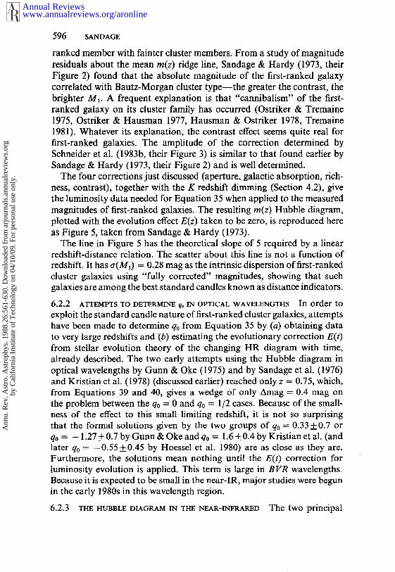
596 SANDAGE

ranked member with fainter cluster members. From a study of magnituderesiduals about the mean re(z) ridge line, Sandage & Hardy (1973, theirFigure 2) found that the absolute magnitude of the first-ranked galaxycorrelated with Bautz=Morgan cluster type--the greater the contrast, thebrighter M~. A frequent explanation is that "cannibalism" of the first-ranked galaxy on its cluster family has occurred (Ostriker & Tremaine1975, Ostriker & Hausman 1977, Hausman & Ostriker 1978, Tremaine1981). Whatever its explanation, the contrast effect seems quite real forfirst-ranked galaxies. The amplitude of the correction determined bySchneider et al. (1983b, their Figure 3) is similar to that found earlier Sandage & Hardy (1973, their Figure 2) and is well determined.

The four corrections just discussed (aperture, galactic absorption, rich-ness, contrast), together with the K redshift dimming (Section 4.2), givethe luminosity data needed for Equation 35 when applied to the measuredmagnitudes of first-ranked galaxies. The resulting re(z) Hubble diagram,plotted with the evolution effect E(z) taken to be zero, is reproduced hereas Figure 5, taken from Sandage & Hardy (1973).

The line in Figure 5 has the theoretical slope of 5 required by a linearredshift-distance relation. The scatter about this line is not a function ofredshift. It has a(M1) = 0.28 mag as the intrinsic dispersion of first-rankedcluster galaxies using "fully corrected" magnitudes, showing that suchgalaxies are among the best standard candles known as distance indicators.

6.2.2 ATTEMPTS TO DETERMINE q0 IN OPTICAL WAVELENGTHS In order toexploit the standard candle nature of first-ranked cluster galaxies, attemptshave been made to determine qo from Equation 35 by (a) obtaining datato very large redshifts and (b) estimating the evolutionary correction E(t)from stellar evolution theory of the changing HR diagram with time,already described. The two early attempts using the Hubble diagram inoptical wavelengths by Gunn & Oke (1975) and by Sandage et al. (1976)and Kristian et al. (1978) (discussed earlier) reached only z = 0.75, which,from Equations 39 and 40, gives a wedge of only Amag = 0.4 mag onthe problem between the q0 = 0 and q0 = 1/2 cases. Because of the small-ness of the effect to this small limiting redshift, it is not so surprisingthat the formal solutions given by the two groups of q0 = 0.33_+0.7 orq0 = -- 1.27 ___ 0.7 by Gunn & Oke and q0 = 1.6 ± 0.4 by Kristian et al. (andlater q0 -- -0.55_+0.45 by Hoessel et al. 1980) are as close as they are.Furthermore, the solutions mean nothing until the E(t) correction forluminosity evolution is applied. This term is large in BVR wavelengths.Because it is expected to be small in the near-IR, major studies were begunin the early 1980s in this wavelength region.

6.2.3 THE F1UBBLE DIAGRAM IN THE NEAR-INFRARED The two principal


Ann

u. R

ev. A

stro

. Ast

roph

ys. 1

988.

26:5

61-6

30. D

ownl

oade

d fr

om a

rjou

rnal

s.an

nual

revi

ews.

org

by C

alif

orni

a In

stitu

te o

f T

echn

olog

y on

04/

10/0

9. F

or p

erso

nal u

se o

nly.



PAST PROPER TIME SAMPLEDt UNIT" I HUBBLE TIME )

0.01 0.02 CLOS 0.10 0.20 0.30

¯ BRIGHTEST GALAXY (83)IN GREAT CLUSTERS

o BRIGHTEST GALAXY (14)iN HMS GROUPS

20l I I I I l8 12 ~6

v£r’_= 48VsM-Kv -/~,v- (BM)- f ( IogNc

F~qure 5 The re(z) fully corrected Hubble diagram for first-ranked E galaxies in clusters.Corrections to magnitudes are made for K dimming, absorption due to the Galaxy, theBautz-Morgan contrast effect, and cluster richness (from Sandage & Hardy 1973).

advantages of observations in the near-IR for large redshifts are (a) thatthe K correction is appreciably smaller than in the B and V wavelengths,and (b) that the E(O evolution term is insensitive to starburst evolution(termed active evolution by Lilly & Longair ! 984). Furthermore, its ampli-tude for passive evolution (i.e. the gradual evolution of the HR diagramof an old coveal population with time) is also much smaller in the K bandthan in the UBV or R bands.

A pioneering advance in K-band photometry was made by Grasdalen(1980) and by Lebofsky (1980), who gave the first re(z) Hubble IRdiagram. Lebofsky (1981), by including radio galaxies, reached z = 1.18and obtained a value of q0 = -0.05+0.30 for z < 0.5, where the E~:(Oevolution term was taken to be zero. A hint for mild evolution for z > 0.5was found even in these early data. More extensive observations (Lebofsky& Eisenhardt 1986) continued to show evidence for mild luminosity evo-lution, consistent with Tinsley’s (1978) predictions.


Ann

u. R

ev. A

stro

. Ast

roph

ys. 1

988.

26:5

61-6

30. D

ownl

oade

d fr

om a

rjou

rnal

s.an

nual

revi

ews.

org

by C

alif

orni

a In

stitu

te o

f T

echn

olog

y on

04/

10/0

9. F

or p

erso

nal u

se o

nly.


598 SANDAGE

Lilly & Longair (1982, 1984) greatly extended the sample using radiogalaxies, reaching z > 1 with a substantial number of objects. They con-cluded that q0 ~ 0.5 if EK(z = 1) = 1 mag, obtained from the (apparent)value of q0 = 3.7 (their Figure 8). They countered a criticism concerningthe use of radio galaxies for their survey by showing no difference in them(z) relation between strong radio sources (using 3C sources, and hencewith radio flux greater than 9 janskys) and weaker 1-jansky sources (Lillyet al. 1985).

These near-IR data gave the first convincing evidence for luminosityevolution in the look-back time to z = 1. A summary of the K data, withthe m(z, E) model lines superposed, is given by Yoshii & Takahara (1988,their Figure 4), shown here as Figure 6. The conclusion from these datais that no model with E = 0 for q0 < 1 fits the near-IR Hubble diagramdata, and therefore that evolution is required, taking the data as theystand.

6.2.zt EVrDENCE FOR LUMINOSITY EVOLUTION FROM THE V-BAND HUBBLE

DIAGRAM Even more powerful evidence that the evolution term E(z) hasbeen detected comes from the work at very large redshifts by Djorgovskiet al. (1985), summarized by Spinrad (1986) and by Spinrad & Djorgovski(1987) using radio galaxies, reaching z = 1.8. Figure 7 is their summaryl-/ubble diagram in V, in which data from a number of authors arecombined. The V magnitudes are as observed, corrected only for apertureeffect (no K correction). Theoretical lines from Equation 35 are shown K term and E(t) evolution according to various Bruzual models are putinto the theoretical model lines, rather than corrections to the obser-vations]. The conclusion is that the data for z > 0.8 cannot be fit by anyq0 value in the no-evolution case [i.e. E(t) = 0], whereas a good fit isobtained with a Bruzual evolving model with qo = 0 and Ho = 50.

A different representation of a subset of these data is shown in Figure8, again taken from Yoshii & Takahara (1988, their Figure 3). As before,the V magnitude is corrected only to the standard metric size for apertureeffect. Again the K redshift dimming and E(t) corrections are put into thetheoretical lines that show q0 and the redshift of galaxy formation in theevolving models; these are shown as the four heavy lines to the left (Ho -- 50km s-1 Mpc-~ is assumed so as to set the time scale of the evolution inthe look-back time). The three lighter lines to the right are for no evolutionfor the q0 = 1, 0.5, and 0.02 cases, none of which fit the data for z > 0.5.The assumed E(t) evolution, as explained earlier, is that given in Figure 2of Yoshii & Takahara (1988), based on work by Arimoto & Yoshii (1986,1987).

The conclusion from Figures 7 and 8 is that evolution must be invoked


Ann

u. R

ev. A

stro

. Ast

roph

ys. 1

988.

26:5

61-6

30. D

ownl

oade

d fr

om a

rjou

rnal

s.an

nual

revi

ews.

org

by C

alif

orni

a In

stitu

te o

f T

echn

olog

y on

04/

10/0

9. F

or p

erso

nal u

se o

nly.


6.0

5.5

5.0

4.5

4.0

3.5


I I I ~ I I I ’ I 5.0

. l,~//. ,.o

O.5

o Lilly ~ ~ngair 119841

~ * Lebofsky (1981} 0.05

~ & Gra~alen

x F~el et al. (19781

8 I0 12 14 IG 18 ~ 220.01

Figure 6 The near-lR Hubble re(z) diagram using K-band magnitudes corrected to a"standard metric" aperture size. The three left-hand theoretical curves are the expectedrelations (Equation 35) for q0 = 1.0 and q0 = 0.5 using the relevant E(t) evolution corrections.The redshift of galaxy formation is marked (z = 3, 5, and 5). The three right-hand curvesare for the marked qo values with no evolution correction. K redshift corrections have been

applied to the theoretical curves rather than the magnitudes (from Yoshii & Takahara 1988).

if the prediction of the standard model (Equation 35) is to be claimed be verified. This is a second demonstration (the first being the observedexcess number counts over the predictions in Figures 3 and 4) that theobservations cannot be used to confirm the simplest standard modelbecause we must "save the phenomenon" by adding evolution. Of course,evolution is expected and, indeed, must be found if the standard model isto be correct because the mean age of the galaxies is required to be afunction of redshift. However, it is important to note that the argument is


Ann

u. R

ev. A

stro

. Ast

roph

ys. 1

988.

26:5

61-6

30. D

ownl

oade

d fr

om a

rjou

rnal

s.an

nual

revi

ews.

org

by C

alif

orni

a In

stitu

te o

f T

echn

olog

y on

04/

10/0

9. F

or p

erso

nal u

se o

nly.


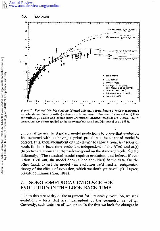
SANDAGE

" ,-’; .............22 I ,~.,i - --.

¯ This work -

m Lilly (~96a)

~ vmd Kri~t.ian ~t a/. (1971~) ._~

¯ ~chneidar ~i sl.¯ H~gs~] {1980)

.2 .4 ~ .8 1 i .2 1.4 1.6 1 .fl ~ ~.2 2 4

Figure 7 The m(z) Hubble diagram (plotted differently from Figure 5, with V ~nagnitudeas ordinate and linearly with z) extended to large redshift. Predicted theoretical re(z) linesfor various q0 values and evolutionary corrections (Bruzual models) are shown. The corrections have been applied to the theoretical curves (from Djorgovski et al. 1985).

circular if we use the standard model predictions to prove that evolutionhas occurred without having a priori proof that the standard model iscorrect. It is, then, incumbent on the claimer to show a consistent series ofneeds for look-back time evolution, independent of the N(m) and re(z)theoretical relations that themselves depend on the standard model. Stateddifferently, "The standard model requires evolution; and indeed, if evo-lution is left out, the model doesn’t [and shouldn’t] fit the data. On theother hand, to test the model with evolution we’d need an independenttheory of the effects of evolution, which we don’t yet have" (D. Layzer,private communication, 1988).

7. NONGEOMETRICAL EVIDENCE FOREVOLUTION IN THE LOOK-BACK TIME

Due to this circularity of the argument for luminosity evolution, we seekevolutionary tests that are independent of the geometry, i.e. of q0-Currently, such tests are of two kinds. In the first we look for changes in


Ann

u. R

ev. A

stro

. Ast

roph

ys. 1

988.

26:5

61-6

30. D

ownl

oade

d fr

om a

rjou

rnal

s.an

nual

revi

ews.

org

by C

alif

orni

a In

stitu

te o

f T

echn

olog

y on

04/

10/0

9. F

or p

erso

nal u

se o

nly.


OBSERVATIONAL TESTS OF WORLD MODELS

Ho = 5Okras=I Mpc"I

MV= -?.3.2 mag

601

5.0

N

o C)jorcjovsky 8= Spinrod (1986)

¯ Kristian et oL (1978)

0.05

3.5 0.01I0 12 14 IG 18 20 22 24 26 28

Vsu(mag)

Figure 8 Same as Figure 6, but for V-band magnitudes (summary diagram from Yoshii Takahara 1988).

the shape of the spectral energy distribution for "standard" galaxies (i.e.of particular Hubble types) at different redshifts. In the second, differencesin the expected morphological mix in particular environments at differentredshifts are queried for possible evolutionary information. A compre-hensive review is given by Kron (1982).

7.1 Changes in Spectral Energy Distribution With Redshift

7.1.1 BROADBAND COLORS Calculations of time-variable evolution werepossible as soon as it was realized that the HR diagram could be explainedby evolutionary tracks off the main sequence rather than up it, andespecially that the Trumpler (1925) cluster classification was an age


Ann

u. R

ev. A

stro

. Ast

roph

ys. 1

988.

26:5

61-6

30. D

ownl

oade

d fr

om a

rjou

rnal

s.an

nual

revi

ews.

org

by C

alif

orni

a In

stitu

te o

f T

echn

olog

y on

04/

10/0

9. F

or p

erso

nal u

se o

nly.


602 SANDAGE

sequence (Sandage 1953, 1957, 1958). Empirical evidence for the changeof color with time of stellar systems that had coeval star formation wasset out from galactic cluster data (Sandage 1963, his Figure 7). The B- colors of the integrated light from any given cluster was found to correlatewell with its age over the age range from 106 to 101° yr.

The effect was successfully modeled by Searle et al. (1973) in what wasone of the first papers on theoretical galaxy evolution, a subject that hasdeveloped into the current flood of detailed studies, often reviewed [e.g.IAU Symposia Nos. 79, 92, 104, and 124, and the Erice workshop ongalaxies at high redshift (Kron & Renzini 1988)].

A principal result of the early work was to show how very slow the colorevolution is with time for old stellar systems. The "observed" rate fromgalactic clusters is A(B- l~)/At _~ 0.03 mag per 109 yr at age ~ 101° yr(Sandage 1963, his Figure 7). This observational result is the same as thetheoretical calculation given earlier by Crampin & Hoyle (1961), whoasked what the colors of M67 would be at earlier ages. The very shallowcolor dependence with old age is also a characteristic of all subsequentreasonable galaxy evolution models, no matter what their level of sophis-tication (cf. Quirk & Tinsley 1973, their Figure 1; Huchra 1977, Larson Tinsley 1978, their Figure 2; Bruzual & Kron 1980, and references therein).

This expected rate of B-- I/change (in the rest wavelength frame) withlook-back time can be transformed into a function of z using Equations36 and 37, which relate z with the evolutionary time for the special casesof q0 = 0 and q0 = 1/2. The age of the q0 = 1/2 model is 13 × 109 yr ifH0 = 50. Redshifts of 0.2, 0.5, and 1.0 have look-back times of 3.1 x 109,

5.9 × 109, and 8.4 x 109 yr, respectively, in this case. Hence, no colorevolution larger than A(B-- 1/) ~_ 0.1 mag is expected for E galaxies untilz > 0.2, after which color effects larger than this should appear.

This expectation is confirmed. Figure 9 shows the observed B-//colorsof first-ranked E galaxies to redshifts as large as z = 0.2 compared withthe predicted color of a standard E galaxy redshifted through the B and//photometric bands. No color evolution has yet occurred. Only afterextension to larger redshifts and to the I~-R color does some colorevolution begin to occur, as expected (Kristian et al. 1978, Djorgovski etal. 1985). The available //-R data are shown in Figure 10. The no-evolution case (the simple Kcorrection applied alone as described in Section4.2) does not fit the data.

These first attempts to find color evolution used broadband photometryof first-ranked cluster E galaxies. In the work of Kristian et al. (1978) thecluster sample was taken from the list of classical clusters known to HMSand from the Abell (1958) catalog, to which they added their sample large-redshift clusters (z ,-~ 0.2-0.7) found in a special search using IIIaJ


Ann

u. R

ev. A

stro

. Ast

roph

ys. 1

988.

26:5

61-6

30. D

ownl

oade

d fr

om a

rjou

rnal

s.an

nual

revi

ews.

org

by C

alif

orni

a In

stitu

te o

f T

echn

olog

y on

04/

10/0

9. F

or p

erso

nal u

se o

nly.



I [ I ~ I ] II

h6-

1.4

o.o 0.08.... 0.,6 0.24L~A/A 0

Figure 9 Observed and predicted B-- I,’, redshift relation for first-rankcd E galaxies (fromOke & Sandage 1968).

Djorgovs~i ~ Spinrad (1986)o Kristion et al. (1978)

O.O 0.2 ~4 0,6 Q8

ZFigure I0 Same as Figure 9 for V-R colors. The theoretical cu~es are for various q0 andredshift fo~ation values using adopted luminosity evolutionary corr~tions. ~e uppercurve is for no evolution of the spectral energy dist~butJon. Evolution Js clearly required bythe data at ~gh redshift (from Yos~i & Takahara 1988).


Ann

u. R

ev. A

stro

. Ast

roph

ys. 1

988.

26:5

61-6

30. D

ownl

oade

d fr

om a

rjou

rnal

s.an

nual

revi

ews.

org

by C

alif

orni

a In

stitu

te o

f T

echn

olog

y on

04/

10/0

9. F

or p

erso

nal u

se o

nly.


604 SANDAGE

photography with the Palomar 48-inch Schmidt telescope (unpublished).A deeper special search by Gunn et al. (1986) lists the most distant clustercandidates yet known, found in a similar survey employing both theSchmidt and the 200-inch Hale reflector.

From an intensive study of Kron’s distant cluster 0016 + 16 (z = 0.54),Koo (1981) used UBVI broadband photometry to demonstrate the exis-tence of many red galaxies that have the nearly normal colors of nearbyE/S0 galaxies, redshifted without appreciable color evolution. Koo citedthe results as a counterexample of the Butcher-Oemler effect (Section7.2.1). However, he later joined with Ellis et al. (1985) to show fromintermediate-band six-color photometry that the mean energy distributionof the E/S0 candidates in this cluster was "significantly bluer than thepresent day equivalent (galaxies) at ultraviolet wavelengths," and thereforethat passive evolution of the spectral energy distribution probably hadoccurred over this look-back time.

However, the effects are small. Contradictory evidence in the field (Koo& Kron 1988a,b) and in other clusters suggests that the rate of evolutionmay not be the same in all E/S0 galaxies in all environments at any givenredshift (Ellis 1988). If so, the evolutionary term E(t) in Equation 35 wouldnot be a unique function of look-back time, even for any given Hubble type.This evolutionary correction to the m(z) Hubble diagram would then bea stochastic variable, and the hope to find q0 by this direct route wouldagain recede as it has so often before.

7.1.2 DETAILED SPECTRAL ENERGY DISTRIBUTIONS Broadband colors dis-advantageously integrate over important details of the spectra that shouldbetray any evolution more sensitively. Oke (1971) obtained spectra three moderately high-redshift galaxies (z = 0.20, 0.38, 0.46) and foundno evidence for evolution in the green and red, but he had no fiducialspectrum in the UV with which to compare over this more sensitive region.Wilkinson & Oke (1978) extended the sample to 56 galaxies and againfound no effect larger than A(B-- V) = 0.04 mag (if that) to the look-backtime corresponding to z = 0.46. They attributed their failure to detect evena small expected effect to variations in the intrinsic properties of the samplegalaxies--they are not all perfect templates of an ideal standard.

The large sample size of the Wilkerson-Oke study gives considerableweight to their conclusions. However, there are hints of evolution in theSEDs of specially selected samples. Spinrad (1986, his Figures 12 and 13)shows that the mean SED of two giant E galaxies at z = 0,2 is redder thanSchild & Oke’s (1971) standard SED for first-ranked E galaxies. He alsofinds that the mean spectra of three giant E’s at z = 0.75 is substantiallybluer in the more sensitive ultraviolet than is the standard. But again,


Ann

u. R

ev. A

stro

. Ast

roph

ys. 1

988.

26:5

61-6

30. D

ownl

oade

d fr

om a

rjou

rnal

s.an

nual

revi

ews.

org

by C

alif

orni

a In

stitu

te o

f T

echn

olog

y on

04/

10/0

9. F

or p

erso

nal u

se o

nly.



contradictory evidence in field galaxy samples [see Koo (1988b) for review] is that little or no color evolution exists in average samples toz ~, 0.4. However, evidence discussed in the next two sections suggests thatthe presence or absence of evolution may depend on the nature of thesample, and that the effects (if present) are likely to be hidden amongstronger selection biases.

7.1.3 THE 4000-h BREAK Bruzual (1983a, his Figure 4), following Spinrad(1977, 1980), presented observational evidence and theoretical models the change in the 4000-/~ spectral discontinuity with time for different starformation rates. The size of this spectral "break" is a moderately sensitivefunction of the spectral type of the mairr sequence termination point(Bruzual 1983a, his Figure 3; Hamilton 1985, his Figure 6). It is alsoknown to be sensitive to metallicity at a given temperature, being the chiefblanketing index for the UV excess given by 6(U- B) (or ml) that measures[Fe/H] for F and G subdwarfs (Roman 1954, Sandage & Eggen 1959,Str6mgren 1966). For these two reasons (age and metallicity) the breakstrength is expected to change with look-back time in some models ofevolution of standard galaxies of a given Hubble type.

Spinrad’s (1986, his Figure 15) data show a pronounced change of breakstrength with redshift for E galaxies in clusters chosen without regard togalaxy color, i.e. simply an "average" galaxy, wherever it could be found.The break change with z observed by Spinrad agrees well with one of thecalculated models by Bruzual.

However, in a remarkable development, Hamilton (1985) applied a rigidcolor selection criterion for a galaxy sample that he used to study theredshift dependence of the break amplitude. In a massive four-color surveythat covered 4 square degrees, composed of eight high-latitude fields,Hamilton picked the reddest galaxies in the sample, using color-colorplots. There was no appeal in the selection to cluster membership becausethe selection criterion was blind to any fact but reddest color. The redshiftrange of Hamilton’s sample was z = 0-0.8. No change of break amplitudewas detected at least to z = 0.6, in contrast to Spinrad’s result for his more"average" sample.

Hamilton’s result shows that very old galaxies exist at z = 0.8 that areat least 2 x 109 yr older than the look-back time of z = 8.7 × 109 yr (ifH0 = 50, q0 = 0). He finds no evidence for either recent star formation orfor passive evolution of the stellar content of this sample. Hamilton’sobserved lack of passive evolution is consistent with his models, but it isnot in agreement with the models of Bruzual. The data prove that at leastsome normal, nonstarbursting E galaxies e~ist at large redshift, and thatthey are old.


Ann

u. R

ev. A

stro

. Ast

roph

ys. 1

988.

26:5

61-6

30. D

ownl

oade

d fr

om a

rjou

rnal

s.an

nual

revi

ews.

org

by C

alif

orni

a In

stitu

te o

f T

echn

olog

y on

04/

10/0

9. F

or p

erso

nal u

se o

nly.


606 SANDAGE

Does Spinrad’s result require evolution for his sample? There is no proofin Spinrad’s data that his sample is composed of normal ellipticals, ratherthan Sa, Sb, or Sc galaxies. It is known that these later types have sys-tematically smaller breaks in local galaxies than in local elliptieals[Hamilton 1985, his Table 2 (from the data of Heckman et al. 1980)].Spinrad’s sample of not necessarily first-ranked cluster galaxies maycontain these later types. The same reason of mixed morphology mightexplain the larger dispersion in break amplitude at a given absolutemagnitude that was found by Dressier & Shectman (1987) in galaxiesin moderately distant clusters but not by Kimble et al. (1987) in localE and SO galaxies in the Virgo cluster,

The conclusion is that secular spectral evolution in the look-back timeto z = 0.8 has not been shown, beyond doubt, from the break data. Aswith the broadband data the results are, as yet, marginal, but the potentialof the method is great.

7.2 Changes in Morphological Mix

7.2.1 rim BUa~CrmR-OEML~R ~r~Eca" A new direction for tests of evo-lution in the look-back time was set out by Butcher & Oemler (1978a,b,1984a,b) in their studies of the fraction of blue galaxies to the total popu-lation of clusters as a function of redshift. They maintain that there isevidence for secular morphologicalevolution in the cores of clusters becausethe blue to red ratio is a progressive function of redshift, starting at thevery low redshift of z -~ 0.15! A large literature has grown covering theeffect, coming down on both sides of the issue. The criticisms that seemedmost serious to Butcher & Oemler were made by Mathieu & Spinrad(1981) and Dressier & Gunn (1982, 1983) concerning cluster membership,and by Wirth & Gallagher (1980) concerning the proper normalization the blue-red ratio in nearby clusters. On the other side, confirmationsupport was given by Couch & Newell (1984), who expanded the sample.These authors also answered a criticism concerning a color bias effect withredshift caused by different Kcorrections for different morphological types(Section 4), a problem raised by DeGioia-Eastwood & Grasdalen (1980).Furthermore, the effect appears not to be present in every cluster; a notableexample is the very compact cluster 0016 ÷ 16 found by Kron (z = 0.54), discussed by Koo (1981). A comprehensive discussion of various selectioneffects that cloud the issue of the reality of the effect is given by Koo(1988a).

7.2.2 7a-m DRESSLER-GUNN EFFECT In a spectroscopic study of theButcher-Oemler effect, Dressier & Gunn (1982, 1983) discovered that thepercentage of emission-line galaxies in distant clusters was higher than in


Ann

u. R

ev. A

stro

. Ast

roph

ys. 1

988.

26:5

61-6

30. D

ownl

oade

d fr

om a

rjou

rnal

s.an

nual

revi

ews.

org

by C

alif

orni

a In

stitu

te o

f T

echn

olog

y on

04/

10/0

9. F

or p

erso

nal u

se o

nly.



control fields at low rcdshift. A literature has also grown on this subjectboth for cluster galaxies and now, with the great recent emphasis, for thefield [scc Ellis (1988) for a review]. Drcssler & Gunn’s discovery has beeninterpreted (Dressier & Gunn 1982, 1983, Drcsslcr 1984) as evidence forrecent (last ~2 × 109 yr) star formation in otherwise "dead" E galaxies.This active evolution is different from the slow passive evolution of oldstellar systems mentioned before. If the abnormal activity occurs in other-wise dead E galaxies, bursts of star formation must be postulated at therelevant look-back time.

But a word of caution is in order. No morphological information ongalaxy types is yet available for the galaxies with active spectra found byDrcsslcr & Gunn. As pointed out by Koo (1988a), Ostcrbrock’s (1984)bias caution may hold the key to explaining the Dresslcr-Gunn statisticsas a selection effect giving a false imprcssion of an emission-line excess inthe field. Scyfcrt galaxies arc among the brightest and bluest galaxies inany volume of space. Hence, in any surveys that arc flux limited, they willdominate the statistics in numbers appearing to increase in percentageover intrinsically fainter galaxies at faint apparent magnitudes. It remainsa problem to determine if this selection bias can affect Dressier and Gunn’sconclusion concerning the unexpectedly strong spectral activity as a func-tion of redshift for field galaxies.

However, much additional work supports the reality of the Dressler-Gunn interpretation of recent starburst activity in some, but not all, other-wise dead ellipticals in clusters with z > 0.3. Ellis (1988) reviews the situ-ation as it appeared in mid-1987. Observations of ,-~ 100 galaxies in Abcllcluster 370 (2 = 0.37) by McLarcn et al. 0988) suggest that UV light fromyoung blue stars has bccn added recently to only 15% of the E galaxies[the remaining 85% remaining normal, reminiscent of Hamilton’s (1985)result]; but in this 15% this is a phenomenon of starbursting that isunknown in local E galaxies observed so far with the IUE satellite, whichagain suggests evolution in the look-back time.

7.3 Reassessment of the N(m) Count Evidence forLuminosity Evolution at z > 0.5 ~-

Faint multicolor photometry of survey fields for the galaxy number countdata is beginning to produce data that will eventually tell if the N(m, qo, E)excess for m > 21 is due to luminosity evolution, i.e. to the E(z) term inEquation 35. Ellis (1988) reviews the enigma that the colors becomesignificantly bluer than expected at magnitude fainter than mj ~ 21 (seealso Kron 1980a, Hamilton 1985), where mj is the J-band magnitude.Furthermore, this is just brightward of where the N(m) counts begin toshow an excess from the predicted curves (Figure 2), an excess that grows


Ann

u. R

ev. A

stro

. Ast

roph

ys. 1

988.

26:5

61-6

30. D

ownl

oade

d fr

om a

rjou

rnal

s.an

nual

revi

ews.

org

by C

alif

orni

a In

stitu

te o

f T

echn

olog

y on

04/

10/0

9. F

or p

erso

nal u

se o

nly.


608 SANDAGE

to a factor of ~ 10 over the model at m~ ~ 26. Recall that this excess hasbeen considered to be strong evidence for luminosity evolution.

However, the mean redshift at mj ,-~ 21 forfield galaxies is only z ~ 0.4,which is so small that no appreciable luminosity evolution is expected inany reasonable galaxy evolution model. This circumstance gives a clue towhat is happening. Spectroscopy is not yet available for complete galaxysamples in the critical magnitude range of rn~ > 21.5 so as to determinethe redshift distribution. However, in an initial redshift survey that iscomplete between 20.0 < mj < 21.5, Broadhurst et al. 0987, as sum-marized by Ellis 1987) found a subset of the complete 200 field galaxysample that was blue and had strong emission lines. A further subset ofthese blue galaxies has a slope of d log N(m)/dm = 0.6 _+ 0.2 for the counts,suggesting that they are nearby and intrinsically faint. If the blue galaxiesare removed from the complete sample, the slope for the remainder of thecounts is dlog N(m)/dm = 0.34 rather than 0.44, causing the excess countsat faint magnitudes in Figure 3 to disappear. Clearly redshifts for the entireblue subset are .required to make a stronger case. However, these datasuggest that luminosity evolution for field galaxies at z "~ 0.4 may not beneeded to explain the N(m) counts. But if so, one of the stronger cases forevolution would disappear.

7.4 Evolution Inferred From Quasar Counts

Two aspects Qf the quasar distribution functions N(m) and N(z) give thestrongest geometrical evidence for evolution.

7.4.1 SLOPE OF THE COUNT-BRIGI-ITNESS RELATION The first evidencefor evolution using optically selected quasars was the pronounced non-Euclidean slope to log N(m) for quasars in the magnitude interval18.1 < B < 21.4 (Sandage & Luyten 1969). The three N(m), mag datapoints of (0.4, 18.1), (5, 19.4), and (100, 21.4) set out by these authors dlogN(m)/dm = 0.75. This is much steeper than 0.6 for nonexpandingEuclidean space. The redshift K correction to the observed magnitude isclose to zero, appropriate for a mean quasar spectrum of v-~ (Sandage1966). The observed slope is steeper than the N(m) relation appropriateto expanding spaces, where dlog N(rn)/dm ,~ 0.4 is predicted from Figure2.

Modern quasar counts, summarized by (among others) Mitchell et al.(1984) at the bright end and by Koo et al (1986, their Figure 7), Koo Kron (1988b), and Boyle et al. (1987, their Figure 1) at the faint confirm these early numbers.

From the count data alone one cannot decide if the evolution is due toluminosity brightening with look-back time or to increased number of


Ann

u. R

ev. A

stro

. Ast

roph

ys. 1

988.

26:5

61-6

30. D

ownl

oade

d fr

om a

rjou

rnal

s.an

nual

revi

ews.

org

by C

alif

orni

a In

stitu

te o

f T

echn

olog

y on

04/

10/0

9. F

or p

erso

nal u

se o

nly.



objects (density evolution). Entrance to the large literature on this problemcan be achieved from Schmidt & Green (1983) and from the review Boyle et al. 0987). The 1987 consensus opinion is that the steep quasarcount-magnitude distribution is due mainly to luminosity evolution.

7.4.2 DECREASE OF dN(z)/dz AT HIGH z The possibility ofa redshift cutoffathigh z (_> 3) was identified early in the analysis of radio quasars listed the 3C Cambridge catalog. Observational selection effects in this radio-selected sample were assessed (Sandage 1972c), and none were found thatcould artificially produce the apparent cutoff, whose cause could be thefirst light from galaxies at high look-back times, i.e. from galaxy creationitself.

In" the ensuing years, the reality of the quasar cutoff has been widelydebated, usually by analyzing optically selected samples that have multipleselection effects not present in the radio samples. A number of deep surveyswere begun early in quest of a cutoff. A review by Smith (1978) of the firstphases of this activity sets the stage for Osmer’s (1982) convincing studyusing optically selected quasars, where he concludes that "the apparentspace density must decrease significantly at 3.7 < z < 4.7."

In an independent deep survey using CCD detection with the Hale200-inch reflector, Schmidt et al. (1986) concur. Their conclusion is that"quasars with an absolute magnitude of MB ~ -- 25 suffer a redshift cutoffnear or below a redshift of 3," A contrary discussion is given by Koo &Kron (1988b), who find no evidence for a redshift cutoff.

Any such large variation (if real) of any property of any type of objectat large redshift is, of course, evidence for secular evolution of meanparameter values with look-back time. Convincing proof would be evi-dence for an evolving rather than a steady-state universe. If indeed evo-lution does occur, it is a most powerful, albeit elementary, verification ofthe most important prediction of the standard model--that the presentUniverse is of finite age. However, if secular evolution cannot be foundwhere it should occur,.the standard model fails. Although there are strongarguments in favor of evolution [Butcher-Oemler, Dressler-Gunn, quagarN(m) slope, perhaps a redshift cutoff for quasars], the data in 1987 arenot yet quite overwhelming.

8. ANGULAR DIAMETER OF RIGID RODS

8.1 The Standard ModelThe theory of the angular diameter of a rigid rod at different distances inan expanding manifold was first worked out by Tolman (1930); it wasdiscussed at greater length in his textbook (Tolman 1934) and also


Ann

u. R

ev. A

stro

. Ast

roph

ys. 1

988.

26:5

61-6

30. D

ownl

oade

d fr

om a

rjou

rnal

s.an

nual

revi

ews.

org

by C

alif

orni

a In

stitu

te o

f T

echn

olog

y on

04/

10/0

9. F

or p

erso

nal u

se o

nly.


610 SANDAGE

Hubble & Tolman (1935) and was put into modern notation by Sandage(1972a), who emphasized the difference between galaxy metric and iso-photal diameters.

Let rR~ be the coordinate interval between the observer and a galaxy atlight emission. Because light rays travel along null geodesics in the expand-ing manifold, the angle 0 between the rays from the extremities of thesource is constant along the light path (neglecting the very small gravi-tational scattering due to intcrvening matter; cL Gunn 1967, Kantowski1969). Hence, upon reception, the angular size of a source of intrinsic sizey (which does not expand with the manifold) is

0 = ~Y~, 43.

or, because Ro = Rt(1 +z),

y(1 +z)0---- 44.

Ror ’

where R0r is the coordinate interval of the source at the time of lightreception given by Equation 30. Hence

0(metric) = (~)q~(1 +z)2

45.qoz + (qo - 1) [- 1 + (1 + 2q0z)

Consider again the two instructive cases of q0 = 1/2 and q0 = 0, whoseR0r values are given by Equations 22 and 26, respectively. Hence, forqo = 1/2,

(~) \(YH°’~2c (1+z)3’246.0 q0-- ;

r./i+z-l~’and for q0 = 0,

0(q0 = 0)= (-~)(1 +z)2 47.

z 1+

Galaxies do not have sharp edges; thus, measurements usually giveisophotal diameters rather than metric. The two are not the same becausein an expanding manifold, surface brightness is not constant with distance.The measured surface brightness is the received (apparent) ttux divided the apparent area, obtained by combining Equations 32 and 44, whichgives


Ann

u. R

ev. A

stro

. Ast

roph

ys. 1

988.

26:5

61-6

30. D

ownl

oade

d fr

om a

rjou

rnal

s.an

nual

revi

ews.

org

by C

alif

orni

a In

stitu

te o

f T

echn

olog

y on

04/

10/0

9. F

or p

erso

nal u

se o

nly.



fb (1 ~_Z)_4, 48.bzindependent of R0r. This means that Equation 48 is model independent,and therefore it does not depend on q0- This famous theorem was firstproved by Tolman (1930). Note that if the manifold is not expanding,Equation 32 has but one (1 +z) factor, and, since R0 = Rj,

SB(nonexpanding) ~ (1 + z)- 49.

The difference between Equations 48 and 49 afford the well-known test (yetto be carried out properly) as to whether the manifold is truly expanding.Because isophotal diameters of galaxies differ from metric as a consequenceof Equation 48, measurement of apparent diameters of galaxies to a givensurface brightness cannot afford a test of Equation 48 (Sandage 1972a,Petrosian 1976, Tinsley 1976).

Suppose, in fact, that the manifold is not expanding and that the redshiftis caused by some sort of energy decay of photons in the path to theobserver. Although no mechanism has yet been proposed to avoid scat-tering of the photon beams in transit, and hence a blurring of distantimages (not observed), nevertheless the predictions of this tired-lighthypothesis are of interest.

Consider that the effect is linear with path length. Obviously then

HRr1 +z = exp --, 50.

C

from which

¢Rr =/_/In (1 +z) 51.

as a guess for flat space. In curved space the distance traveled is not Rrbut rather R sin (HRr/c) for k = + 1 and R sinh (HRr/c) for k = --1.Hence, in the case where the curvature factor is set to HR/c = 1 we havethe possibilities

O= yH°-[ln(l+z)]-I for k=0, 52.C

o=YH°--{sin[ln(l+z)]}-I for k= +1, 53.

o=YH°{sinh[ln(l+z)]}-I for k=--l. 54.


Ann

u. R

ev. A

stro

. Ast

roph

ys. 1

988.

26:5

61-6

30. D

ownl

oade

d fr

om a

rjou

rnal

s.an

nual

revi

ews.

org

by C

alif

orni

a In

stitu

te o

f T

echn

olog

y on

04/

10/0

9. F

or p

erso

nal u

se o

nly.


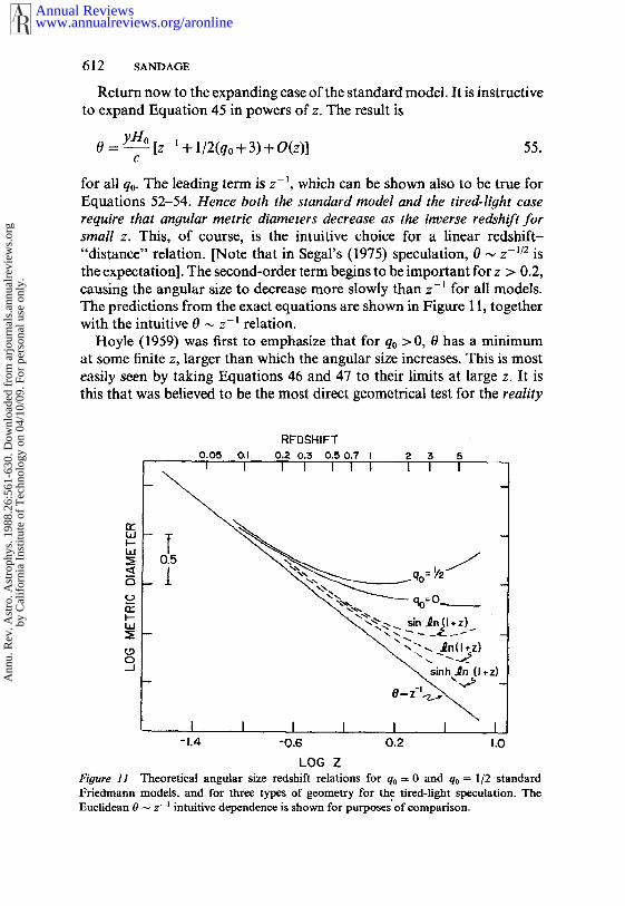
612 SANDAGE

Return now to the expanding case of the standard model. It is instructiveto expand Equation 45 in powers of z. The result is

0 = yH___~o [z- ~ + 1/2(q0 + 3) + O(z)] 55.c

for all q0- The leading term is z 1, which can be shown also to be true forEquations 52-54. Hence both the standard model and the tired-light caserequire that angular metric diameters decrease as the inverse redshift forsmall z. This, of course, is the intuitive choice for a linear redshift-"distance" relation. [Note that in Segal’s (1975) speculation, 0 ,,~ z-1/2 isthe expectation]. The second-order term begins to be important for z > 0.2,causing the angular size to decrease more slowly than z-~ for all models.The predictions from the exact equations are shown in Figure 11, togetherwith the intuitive 0 ,-~ z-~ relation.

Hoyle (1959) was first to emphasize that for q0 >0, 0 has a minimumat some finite z, larger than which the angular size increases. This is mosteasily seen by taking Equations 46 and 47 to their limits at large z. It isthis that was believed to be the most direct geometrical test for the reality

REDSHIFTo.o5 o.I o.z 0.3 0.5 0.7 ~ 2 3 5~ I I I I I I I I I

Ld

Ld

_~ _

--I nh~n (I ~z)

-1.4 -0.6 0,2 1.0LOGZ

Fit~ure ]1 Theoretical angular size-redshiftrelations for q0 = 0 and q0 = 1/2 standardFriedmann models, and for three types of geometry for the tired-light speculation. TheEuclidean 0 ~ z-~ intuitive dependence is shown for purposes of comparison.


Ann

u. R

ev. A

stro

. Ast

roph

ys. 1

988.

26:5

61-6

30. D

ownl

oade

d fr

om a

rjou

rnal

s.an

nual

revi

ews.

org

by C

alif

orni

a In

stitu

te o

f T

echn

olog

y on

04/

10/0

9. F

or p

erso

nal u

se o

nly.



ofexpandin# space. The effect has been sought in many observational tests(Section 8.3) but has not been found, raising what is the most seriousdoubt to date about the standard model because it questions whether theredshift is due to real expansion. Again, to save the phenomenon we mustinvoke evolution of the size of the standard rod in the look-back time.Before discussing the data at large look-back times, consider first the dataat low redshift to test the leading term in the series expansions of Equations45-47 and 52-54.

8.2 Diameters of First-Ranked ClusterGalaxies at Low Redshift

To test the 2-~ dependence of Equation 45 at low redshift requires onlya crude experiment. Furthermore, in this regime, isophotal and metricdiameters are nearly the same. A photographic test made in 1970-71 usingeye estimates of the angular diameters from Palomar Schmidt and 200-inch plates (Sandag¢ 1972a) was sufficient to show that the dependenceon _7 is Z-I, as in Equation 55. The data, set out in Figure 12, range inredshift from 2 -- 0.0023 for the Leo group to 2 = 0.46 for 3C 295. Overthis range, the isophotal diameters (to an isophote of ,-~ 23 mag arcsec-2)

range from ~ 250 arcsec to ~ 2 arcsec.

5.0

4.5

o 4.00

3.5

3" I0" 30" I00" 300"I

0.333

~ 0.100

Z0.033

0.010

0.003

I i [ i1.2 2.0

LOG 8 (sec)

o 200- INCH

3.0 -- ¯ 48- INCH

0.4

Figure 12 The observed O(z) relation for low-redshift, first-ranked E cluster galaxies

obtained by eye estimates from a homogeneous set of photographic plates. The line is the

0 ~ z-l Euclidean expectation (from Sandage 1972a).


Ann

u. R

ev. A

stro

. Ast

roph

ys. 1

988.

26:5

61-6

30. D

ownl

oade

d fr

om a

rjou

rnal

s.an

nual

revi

ews.

org

by C

alif

orni

a In

stitu

te o

f T

echn

olog

y on

04/

10/0

9. F

or p

erso

nal u

se o

nly.


614 SANDAGE

This test of the linearity of the redshift-distancc relation is independentof the re(z) test of Section 4, although it is related to re(z) under theassumption that all first-ranked E galaxies have only a small dispersion insurface brightness about a mean value. In the quoted paper, I called thispremise the "constant" surface brightness condition, to which Gudehus0975) pointed out the more proper statement now given--to wit, that stable mean surface brightness with small dispersion exists that is inde-pendent of rcdshift at low rcdshift.

8.3 High-Redshift Data

8.3.1 RADIO SOURCES Hoyle’s (1959) prediction of a minimum in 0 at redshift of z = 5/4 for q0 = 1/2 (and similar m~nima for other q0 > 0) hasbeen searched for extensively. Miley 0968, 1971) was among the first toapply the test to double-lobe radio sources, showing that they obey a z-1relation over the entire rcdshift range that reaches z = 2. Selection cffcctswere invoked to explain the lack of turnup of O(z). Because the radiosources are from a catalog that is limited to a given (bright) radio fluxlevel, there is a strong variation of absolute radio power with redshift(Sandage 1972c, his Figure 7). Hence, if the linear separation of the radiolobes varics with power, the observed z might bc explained. Note thatbecause O(z) is smaller than expected at large redshift, such an explanationrequires that ~he more powerful radio emitters have the smaller lineardimensions. (Those at largest z have the highest power due to the fluxlimitation of the source catalog.)

Following Miley 0968, 1971), the data discussed by Lcgg (1970),Wardle & Miley (1974), Swarup (1975), and Kapahi (1975, 1985) tinued to show the same problem. Kapahi’s 0987, his Figure 7) compre-hcnsivc revicw of the most recent data again shows the nccd for size evo-lution of the sources, probably with look-back time rather than withradio power, to save the standard model.

8.3.2 CLUSTERS OF GALAXIES The variation with rcdshift of a charac-teristic angular size of clusters of galaxies has been sought. Various defi-nitions of "size" have been proposed. The most complete study is that byHickson (1977a,b), who used the harmonic mean separation of the bright-cst 40 galaxies within a specified radius from the center. The problem withthis definition is that the specified radius of 3 Mpc depends on q0 at largercdshift. Bruzual & Spinrad 0978) show the partial degeneracy of thisaperture-size problem to the galaxy selection with which to form theharmonic mean. Hickson (1977b; see also Hickson & Adams 1979) correctsfor this effect by using the results of Monte Carlo simulations in thepresence of field galaxies of given surface density, but the correction is


Ann

u. R

ev. A

stro

. Ast

roph

ys. 1

988.

26:5

61-6

30. D

ownl

oade

d fr

om a

rjou

rnal

s.an

nual

revi

ews.

org

by C

alif

orni

a In

stitu

te o

f T

echn

olog

y on

04/

10/0

9. F

or p

erso

nal u

se o

nly.



model dependent. Bruzual & Spinrad choose to analyze their independentdata by fitting a theoretical density profile to galaxy counts so as todetermine a core radius for each cluster, a method similar to that used byBahcall [see Bahcall (1977) for a review].

In an analysis of both sets of data, Hickson & Adams (1979) concludethat "evolution in the linear cluster sizes is required for agreement with[the] models. Unless q0 is considerably greater than 1, the mean clustersize is decreasing (i.e. evolving) at present with a time scale comparableto Hb- ~." The combined data from the two studies, uncorrected for evo-lution, are shown in Figure 13 as set out by Hickson & Adams (1979, theirTable 1). The data of Bruzual & Spinrad are closer to the Friedmann linesof q0 = 0 and q0 = 1/2 than those ofHickson & Adams (note the systematicdifference of the two data sets at large redshift).

To first order, the z-1 dependence at small redshifts is again clearlyevident in the data. However, for the second-order effect (i.e. the q0 depen-dence) it is less certain that the data can even be meanit~gful because of thegrowing suspicion that clusters are not well-defined structures that havereached dynamic equilibrium. Most clusters appear to be young aggregates,still in the process of formation. The evidence comes from data on theVirgo cluster (Tully & Shaya 1984, Binggeli et al. 1987) and from thepresence of substructure (multiple condensations) in most clusters studiedin detail [Geller & Beers E$82, Baier 1983 (with many references to theearlier observational data), Beers & Tonry 1986]. Most important is theDressier (1980) morphology-density effect within a given cluster, showingthat virial mixing has not occurred.

With such pronounced subclustering, the meaning of the core radius orany other similar parameter becomes vague, depending on details of theforming cluster clumps. Measurement of the second-order curvature effect(i.e. q0) using such an evolving metric rod must be questioned, despite itspower to determine the gross first-order term.

8.3.3 METRIC DIAMETERS OF FIRST-RANKED CLUSTER GALAXIES It can beargued that the diameters of the brightest E galaxies in clusters are morestable than the sizes of the radio lobes of active galaxies or the sizes ofclusters that are just forming. The evidence is the tightness of the m(z)Hubble diagram (Figure 5) despite the question of cannibalism (Section6.2.1), unless the cannibals operate with an effect that has an almostdispersionless progression with redshift. (In principle, cannibalism can bestudied by finding different cannibal rates in clusters of different density.)

Metric diameters must be used in a test of Equation 48. Petrosian’s(1976) definition of a metric diameter (his ~/index) has many advantages,such as its being nearly independent of luminosity evolution, of K correc-


Ann

u. R

ev. A

stro

. Ast

roph

ys. 1

988.

26:5

61-6

30. D

ownl

oade

d fr

om a

rjou

rnal

s.an

nual

revi

ews.

org

by C

alif

orni

a In

stitu

te o

f T

echn

olog

y on

04/

10/0

9. F

or p

erso

nal u

se o

nly.

616 SANDAGE


Ann

u. R

ev. A

stro

. Ast

roph

ys. 1

988.

26:5

61-6

30. D

ownl

oade

d fr

om a

rjou

rnal

s.an

nual

revi

ews.

org

by C

alif

orni

a In

stitu

te o

f T

echn

olog

y on

04/

10/0

9. F

or p

erso

nal u

se o

nly.



tion, and of the wavelength of observation. It is defined as the radius inthe image at which the ratio of surface brightness, averaged over the areainterior to that radius, to the SB at that radius is an adopted fixed number.Because it is a ratio, many corrections cancel.

Other examples of metric measures of size are the radius that containshalf the light (called the "effective radius" in the literature); the Hubble radius, where the SB falls to one fourth its "central" value; and the Kingcore radius, where the SB is one half the "central" value. Central SB isnever measured because of finite seeing disks, but a fitting parameter (I0)can be inferred from global fits of the intermediate profile (i.e. for radiiappropriately larger than the seeing disk).

A literature exists (cf. Oemler 1976, Kormendy 1977, Schombert 1986,Hoessel et al. 1987) on how some of these measures of radii vary with MBof the parent galaxy and of the dispersion about the mean correlation, butno large study yet exists of the stability of the Petrosian ~/index for localgalaxies. If it proves to b¢ stable at some optimum SB ratio, the way wouldbe open to test Equation 48 at large rcdshift. This is the only known testfor the reality of the redshift, hence its extreme importance. The test hasbeen tried by Geller & Peebles (1972), but it can be argued that they usedisophotal rather than metric diameters, and further that they had onlyfour data points.

Progress toward practical use of the Petrosian size has been reported byDjorgovski & Spinrad (1981). They measured the diameters of distantgalaxies up to z = 1.17, but with only a few clusters to define the brightend. Their preliminary result is that the data, as measured, do not fit anypart of the standard model parameter space (with A = 0), and that to so again requires application of an evolutionary correction to the first-ranked galaxy sizes as a function of redshift. If the evolution is due tocannibalism, it can in principle be corrected by making the measurementson lower-ranked (fainter) cluster members that have not partaken of thecannibal’s feast.

The chief observational problem at the moment is that the angulardiameter where r/= 2 mag is ~ 2 arcsee at z = 1; this is subject then toseeing corrections from the ground in order to obtain a proper r/value atthis redshift.

9. TIME-SCALE TEST

9.1 The Standard Model Prediction

The value of the redshift-distance ratio (i.e. the Hubble constant) was firstset at H0 = 558 +__ 10% km s-~ Mpc-1 (Hubble & Humason 1931). Usingthis determination it was soon evident that the redshift of the galaxies is


Ann

u. R

ev. A

stro

. Ast

roph

ys. 1

988.

26:5

61-6

30. D

ownl

oade

d fr

om a

rjou

rnal

s.an

nual

revi

ews.

org

by C

alif

orni

a In

stitu

te o

f T

echn

olog

y on

04/

10/0

9. F

or p

erso

nal u

se o

nly.


618 SANDAGE

a characteristic of the Universe itself, rather than being simply a localphenomenon. The evidence is the order-of-magnitude agreement betweenthe expansion time scale associated with Hff~ (which is 1.7 x 109 yr forH0 = 558) and the age of the Earth, known even at the beginning of thiscentury to be of order l09 yr [Holmes (1913), and many times thereafterfollowing Boltwood (1907); cf. Holmes 0946, 1947, 1949) and Jeffreys(1924, 1948, 1949) for the early literature].

The conclusion was strengthened when the age of the oldest stars in theGalaxy was shown to be of the same order (Sandage & Schwarzschild1952). This followed the earlier, several-decade debate on two time scalesfor the Galaxy. Bok (1946) reviewed the multiple evidence for the longand short time scale. Note from his review that even in 1946, evolution ofstars was considered to be up rather than offthe main sequence, giving nocharacteristic signal in the HR diagram by which to date the stars. Thisdifficulty prevailed until Trumpler’s 0925, 1928) discovery of mainsequence termination points was theoretically understood in the early1950s with the introduction of chemically inhomogeneous stellar models.

A third time scale was proposed by Rutherford (1929) that permittedage dating oi~ the chemical elements. Ages of several times 109 yr foruranium was close enough to the Hubble time to be startling. In moderntimes the theme has been integrated into a general history of events thathave spread the elements made in stars everywhere that there is matter(Hoyle 1946, 1947, 1954, Burbridge et al. 1957), setting the foundationsfor the study of the chemical evolution of galaxies.

Although order-of-magnitude agreement of the three cosmic clocksdraws attention to the significance of the time-scale coincidence, a moredetailed inquiry requires precision in the measurements. The standardmodel predicts the relation between the age of the Universe To, the Hubbleconstant H0, and cosmological parameters q0 (or fl0) and A. Many rep-resentations of this parameter space exist, such as that of Robcrtson(1955, 1963) for a specific value of H0; of Fowler (1987), who generalizedRobertson’s parametrization by using D.o and HoTo as axes; or of Stabell& Refsdal (1966, their Figure 5) in the density, q0 plane with HoTo asparameter.

Figure 14 (from Sandage & Tammann 1986) is a diagram in the HoTo, Aplane with f~0 as parameter, plotted from the tables of Refsdal et al. (1967)following Mattig (1958) and Solheim (1966). The well-known conditionthat To = 2/3H~ ~ if fl0 = 1 and A = 0 is marked by a crossed circle. Twoother data points are marked by filled circles at values of H0 and Tothought, in various past discussions, to be appropriate. The point to noteabout Figure 14 is that HoTo, which is in principle observable, permits O-oto be determined if A is known (or assumed); conversely, it permits A


Ann

u. R

ev. A

stro

. Ast

roph

ys. 1

988.

26:5

61-6

30. D

ownl

oade

d fr

om a

rjou

rnal

s.an

nual

revi

ews.

org

by C

alif

orni

a In

stitu

te o

f T

echn

olog

y on

04/

10/0

9. F

or p

erso

nal u

se o

nly.



4

3

2

!

-!

I I I I I I I

POSSIBLEI-Io=50TO = 24 x 109y,0,0=0.15

c~’,6. =0.9 H0 = 50

TO =18.3 xlOs

,0.0= 0.15

I t t I I I I I I ~2.0 1.8 1.6 ! .4 1.2 t.0 0.8 0.6 0.4 0.2

HoTo

Figure 14 The time-scale test displayed in the HoTo, A plane with ~0 as parameter. The flatspace-time condition of Ac~ = 3Ho~(1-D~) is shown by the heavy line marked K= 0. Thespecial case of D~ = l, A = 0, HoTo = 2/3 is marked by a crossed circle (from Sandage Tammann 1986).

be found if HoT0 and D-0 are known. The special cut at A = 0 in the diagramgives the D.0 =f(HoTo) relation calculated earlier (Sandage 1961a, Table8).

9.2 The Value of To From the Chemical Elementsand From the Oldest StarsTo use Figure 14 requires a knowledge of H0 and the age of the Universe,found independently of the expansion data. The two methods to measureTo are (a) use of the age of the oldest stars in the Galaxy (to which gestation time of galaxies is added), and (b) a determination of the age the chemical elements. Entrance to the large literature on the second


Ann

u. R

ev. A

stro

. Ast

roph

ys. 1

988.

26:5

61-6

30. D

ownl

oade

d fr

om a

rjou

rnal

s.an

nual

revi

ews.

org

by C

alif

orni

a In

stitu

te o

f T

echn

olog

y on

04/

10/0

9. F

or p

erso

nal u

se o

nly.


620 SANDAGE

problem is available in Burbidge et al. (1957), Dicke (1969), Cameron(1982), Fowler (1984), Thielemann & Truran (1986), Butcher (1987),Clayton (1987), and Cowan et al. (1987). The range in age in these erences is wide, between ~9 x 109 and ~25 x 109 yr depending onassumptions such as sudden synthesis or gradual enrichment. Strongerstatements on narrower limits enhance the literature, but no one has deniedthat the problem is model dependent in a way that is difficult to check. Aforceful review that favors the short end of this range can be enjoyed fromFowler (1987).

The astronomical age dating of the Galaxy comes from measured globu-lar cluster main sequence termination points, combined with stellar evo-lutionary model calculations for various helium and metal chemical com-positions. Age estimates became stabilized in the early 1980s near 17 × 109yr, based on generally accepted values of the chemical composition, theabsolute magnitude Mv of the horizontal branches to set the terminationluminosity, and models calculated by three principal groups (cf. Iben Rood 1970, Ciardullo & Demarque 1977, VandenBerg 1983). The meanage of ,-~ 17 Gyr from the Yale (or VandenBerg) isochrones was based distance moduli that use My = 0.63 mag for P,R Lyrae stars of O~terhoffgroup II globular clusters and My = 0.80 mag for those of group I (Sandage1982).

In a new development, observational evidence is becoming persuasivethat the O/Fe chemical abundance ratio does not track with the Fe/H ratioin field subdwarfs of various Fe/H metallicities. An extensive review of theevidence is found in the ESO 1985 Workshop on Production and DistributionofC, N,O Elements, edited by Danziger et al. (1985). Following Simoda Iben (1970), recent analyses by VandenBerg (1987), P. Demarque (privatecommunication, 1987), and Rood & Crocker (1985) have independentlyshown that if the oxygen abundance remains high as the Fe/H ratiodecreases, the age for a given turnoff luminosity decreases in the sameway it would have decreased if Fe/H were increased. VandenBerg (1987)estimates that ages of globular clusters must be decreased by ,~ 15% fromthe earlier values due to this effect of enhanced oxygen abundance inotherwise metal-poor stars if the effect in field subdwarfs occurs in globularcluster main sequence stars (but see Pilachowski 1988).

From this evidence and from a precision measurement of the age of 47Tuc (Hesser et al. 1987), and adding 1.4 Gyr for the gestation time of theGalaxy, Sandage (1988a) adopted

To = 14.9___2Gyr

for the age of the Universe from the age dating of stars.


Ann

u. R

ev. A

stro

. Ast

roph

ys. 1

988.

26:5

61-6

30. D

ownl

oade

d fr

om a

rjou

rnal

s.an

nual

revi

ews.

org

by C

alif

orni

a In

stitu

te o

f T

echn

olog

y on

04/

10/0

9. F

or p

erso

nal u

se o

nly.



9.3 Value of rio

In these pages Hodge (1981) reviewed the debate up to ~ 1980 on thevalue of the Hubble constant, giving extensive references. Since that timeattempts have been made to discover the source of the factor of 2 differencein H0 between the long- and the short-distance scale workers. A factor of2 in distance at a given redshift is equivalent to 1.5 magnitude (factorof 4 in luminosity). The source of the discrepancy must be sought andconvincingly found if the matter is to be put to rest while members of thepresent generation are still active.

The factor of 2 is not in the local calibrators (Tammann 1987a,b), whereat most only ~0.3 mag separates the various adopted calibrations. Theexplanation is almost certainly to be found as bias effects in the analysisof data from flux-limited catalogs, no matter what distance indicator isadopted, if that indicator is anything other than redshift. The proof of thisstatement is the apparent increase ofH o with redshift, ranging from 50 kms-1 Mpc-1 locally to > 100 at ~4 times the Virgo cluster, obtained in allof the analyses by the advocates of the short scale (cf. de Vaucouleurs Peters 1986, their Figure 2; Giraud 1986a,b, 1987). Discussions of this biasand why the apparent increase of H0 with distance is an artifact includethose by Teerikorpi (1975a,b, 1984, 1987), Sandage et al. (1979), Bottinelliet al. (see their 1987 and 1988 papers for a review), Kraan-Korteweg al. (1986, 1988), and Sandage (1988a,b).

There have been many ways to discuss this type of Malmquist bias influx-limited samples, most of which are complicated enough to be butdimly understood except, perhaps, by their authors. Figure 15 illustratesstill another discussion of the effect and its consequences. Shown is aschematic re(z) Hubble diagram using objects that have a spread in abso-lute magnitude M. Parallel envelope lines drawn to encompass the sampledefine the loci of absolute magnitudes M1 and M2. (For a linear velocity-distance relation, recall that the slope of these lines is dm/dlogz = 5.)Divide the data into redshift zones, labeled 1-10 and shown hatched inFigure 15. If the sample is taken from a magnitude-limited catalog, therewill be a limit line as shown, for which no objects in the sample are fainter.Consider now the mean (ridge) line of the data sample in the z,m plane.The true mean (M.r) value is seen in the data up to distance interval 4--5,but beyond that the data begin to be systematically too bright comparedwith the true value of

What are the consequences? Suppose we assign an absolute magnitude(My) to each galaxy in the sample. For those closer than distance interval5-6 we will make as many positive as negative errors in the correct m- Mdistance modulus due to the luminosity spread in M. This part of the


Ann

u. R

ev. A

stro

. Ast

roph

ys. 1

988.

26:5

61-6

30. D

ownl

oade

d fr

om a

rjou

rnal

s.an

nual

revi

ews.

org

by C

alif

orni

a In

stitu

te o

f T

echn

olog

y on

04/

10/0

9. F

or p

erso

nal u

se o

nly.


622 SANDAGE

EFFECT OF CATALOGFLUX LIMITATION

ON

Mz

DENIED

3ATALOGLIMIT

APPARENT MAGNITUDE

Figure 15 Illustration of the Malmquist bias as it affects the m(z) Hubble diagram. Upper-and lower-envelope lines are shown that enclose the sample. The absolute magnitude Mt isbrighter than M2. The mean absolute magnitudes of the subsamples (crosses indicated ateach distance interval) become progressively brighter with distance than the (M) value thatapplies to a complete (volume-limited) sample, valid for the data closer than distance limitnumber 5,

sample is distance limited. However, the flux limitation of the faintersample progressively removes fainter absolute magnitudes from theremaining set as the true distance increases, giving false (biased) meanm-M values. The inferred distances are too small in the mean for thissubsample (because the (M~r~ used is too faint to apply to it, as shown the position of the crosses). By using these incorrect inferred photometricdistances to obtain Ho, progressively larger (incorrect) values of H0 wouldbe obtained as an artifact. Note that the correct value of H0 is that obtainedonly in the distance interval closer than 5-6.

Detailed analysis of actual data (Sandage 1988a,b) has shown this biasexplicitly in samples of ScI galaxies and in galaxies used for the Tully-Fisher distance scale method. By reading the data in the redshift limit ofz -~ 0, low values of H0 have been obtained using the local calibratorswith Cepheid distances. This is equivalent to the method of Richter &Huchtmeier (1984), who restrict their sample to the distance-limited listof Kraan-Korteweg & Tammann (1979) and obtain a low value of directly (cf. Sandage 1988b).


Ann

u. R

ev. A

stro

. Ast

roph

ys. 1

988.

26:5

61-6

30. D

ownl

oade

d fr

om a

rjou

rnal

s.an

nual

revi

ews.

org

by C

alif

orni

a In

stitu

te o

f T

echn

olog

y on

04/

10/0

9. F

or p

erso

nal u

se o

nly.



From these studies, together with a cluster data analysis with the Tully-Fisher method (Kraan-Korteweg et al. 1988), the value of the Hubbleconstant has been found to be in the range

42 _< H0 ~< 57kms-1Mpc- l,

where the formal error is adopted to be ~ + 10% from individual studies.The value found from supernovae of type Ia, using both an empirical(Sandage & Tammann 1982) and a theoretical calibration (Sutherland Wheeler 1984, Arnett et al. 1985) of the absolute magnitude, gives(Cadonau et al. 1985)

H0 -- 43 _+ 10km s- 1 Mpc- 1, 56.

which in turn gives a Hubble time of Hfft --- 22.7 + 5.5 Gyr.

9.4 The Time Test of the Standard Model

of the four tests discussed earlier IN(z), N(m), m(z), 0(z)], the time testfor q0 is the only experiment devoid of direct evolutionary effects, makingit the most promising (at the moment) to find q0 (or D,0 ifA = 0). AdoptingHo = 42-t- 11 km s-1 Mpc-1 and To = 14.9_+2 Gyr (Sandage 1988a) gives

ToHo -- 0.64_+0.19,

which is the close to the required 2/3 if f2o = 4-1. The formal solution is

~q0 1 -~+ 3.0 57.~ .~-- 0.9,

where the formal errors depend mostly on the large assigned error to Ho.If we assign a smaller error and adopt H0 = 42_+ 6, then

~0 1 2+ 1.6~ ¯ -I).7

Although the errors are still very large, there is now, for the first time, theastronomical possibility that D.0 = 1 exactly, required by the inflationarycosmology of Grand Unification. It must be emphasized, however, thatno claim is made here from the available data that fl0 is 1, only that it isnow possible that it could be so if H0 can be reduced, as here, to 42 andTo shortened by ,-, 15% below 17 Gyr. This does give agreement withthe inflationary prediction from the time-scale test, whereas the earlierliterature values on ages did not.

Equation 31 shows that the price to be paid is to believe that at least99% of the matter in the Universe is dark. Such dark matter has not yetbeen detected, and its existence must remain an article of faith for thetrue believer in the standard model and its covering theory of GrandUnification.


Ann

u. R

ev. A

stro

. Ast

roph

ys. 1

988.

26:5

61-6

30. D

ownl

oade

d fr

om a

rjou

rnal

s.an

nual

revi

ews.

org

by C

alif

orni

a In

stitu

te o

f T

echn

olog

y on

04/

10/0

9. F

or p

erso

nal u

se o

nly.


624 SANDAGE

ACKNOWLEDGMENTS

This review is partially based on class notes from a lecture series on

cosmology given at The Johns Hopkins University in the spring of 1987.

It is a pleasure to thank the Department of Physics and Astronomy at

JHU for the opportunity to lecture and to organize this work. JanetKrupsaw of JHU prepared an early version of part of the manuscript with

her usual enthusiasm and skill. It is also a pleasure to thank Susan Drescher

of the Mount Wilson and Las Campanas Observatories for her cheerful

and careful preparation of so many drafts of the final manuscript. Special

thanks are due David Layzer, who carefully read an early draft and madea number of suggestions to modify parts of the philosophical framework,

and who also corrected misstatements of principle. Not all of his sugges-

tions were taken, and remaining errors are claimed here by their owner.

It is again a pleasure to acknowledge and to thank Keith Dodson ofAnnual Reviews for his careful, sensitive, and excellent job of textual

editing.

Literature Cited

Abell, G. 1958. Ap. J. Suppl. 3:211Alpher, R. A. 1948. Phys. Rev. 74:1577Alpher, R. A., Bethe, H. A., Gamow, G.

1948. Phys. Rev. 73:803Alpher, R. A., Folin, J. W., Herman, R. C.

1953. Phys. Re~. 92:1347Alpher, R. A., Herman, R. C. 1948. Phys.

Re~. 74:1737Alpher, R. A., Herman, R. C. 1950. Rev.

Mod. Phys. 22:153Arimoto, N., Yoshii, Y. 1986. Astron. Astro-

phys. 164:260Admoto, N., Yoshii, Y. 1987. Astron. Astro-

phys. 173:23Arnett, W. D., Branch, D., Wheeler, J, C.

1985. Nature 314:337Backer, D. C., Hellings, R. W. 1986. Ann.

Rev. ,4stron. Astrophys. 24:537Bahcall, N. 1977. Ann. Rev. Astron. Astro-

phys. 15:505Baier, F. W. 1983. Astron. Nachr. 304:211Balian, R., Audouze, J., Schramm, D. N.,

eds. 1979. Physical Cosmology. Les Hou-ches Summer Sch. No. 22. Amsterdam:North-Holland

Bautz, L. P., Morgan, W. W. 1970. Ap. J.Lett. 162:L149

Beers, T. C., Tonry, J. L. 1986. Ap. J. 300:557

Binggeli, B. 1987. In Nearly Normal Gabaxles, ed. S. Faber, p. 195. New York:Springer-Verlag

Binggeti, B., Sandage, A., Tam_mann, G. A.1988. Ann. Rev. Astron. Astrophys. 26:509

Binggeli, B., Tammann, (3. A., Sandage, A.1987. Astron. J. 94:251

Boesgaard, A. M., Steigman, G. 1985. Ann.Rev. Astron. Astrophys, 23:319

Bok, B. J. 1931. Harvard Circ. No. 371Bok, B. J. 1934. Harvard Bull. No. 895Bok, B. J. 1937. Distribution of Stars in

Space, p. 26-37. Chicago: Univ. ChicagoPress

Bok, B. J. 1946. MNRAS 106:61Boltwood, B. B. 1907. Am. J. Sci. 23:77¯ Bottinelli, L., Fougue, P., Gouguenheirn, L.,

Paturel, G, Teerikorpi, P. 1987. Astron.Astrophys. 181:1

Bottinelli, L., Gouguenheim, L., Paturel, G.,Teerikorpi, P. 1986. Astron. Astrophys.156:157

Bottinelli, L., Gouguenheim, L., Paturel, G.,Teerikorpi, P. 1988. Ap. J. 328:4

Boyle, B. J., Shanks, T., Fong, R., Peterson,B. A. 1987. In Observational Cosmology,1AU Syrup. No. 124, ed. A, Hewitt, G.Burbidge, L.-Z. Fang, p. 643. Dordrecht:Reidel

Broadhurst, T. J., Ellis, R. S., Shanks, T.1987. MNRAS. In press

Brown, (3. S., Tinsley, B. M. 1974. Ap. J.194:555

Bruck, FI. A., Coyne, G. V., Longair, M.


Ann

u. R

ev. A

stro

. Ast

roph

ys. 1

988.

26:5

61-6

30. D

ownl

oade

d fr

om a

rjou

rnal

s.an

nual

revi

ews.

org

by C

alif

orni

a In

stitu

te o

f T

echn

olog

y on

04/

10/0

9. F

or p

erso

nal u

se o

nly.



S., eds. 1982. Astrophysical Cosmology. deSitter, W. 1917. MNRAS78:3Pontif. Acad. Sci. Scr. Varia. No. 48

Bruzual, A. G. 1981. Rev. Mex. Astron.Astrofis. 6:19

Bruzual, A. G. 1983a. Ap. J. 273:105BruzuaL A. G. 1983b. Rev. Mex. Astron.

Aslrofis. 8:63Bruzual, A. G., Kron, R. G. 1980. Ap. J.

241:25Bruzual, A. G., Spinrad, H. 1978. Ap. J. 220:

IBurbidge, E. M., Burbidge, G. R., Fowler,

W. A., Hoyle, F. 1957. Rev. Mod. Phys.29:547

Butcher, H. 1987. Nature 328:127Butcher, H., Oemler, A. 1978a. Ap. J. 219:

18Butcher, H., Oemler, A. 1978b. Ap. J. 226:

559Butcher, H., Oemler, A. 1984a. Ap. J. 285:

426Butcher, H., Oemler, A. 1984b. Nature 310:

31Cadonau, R., Sandage, A., Tammann, C~.

A. 1985. In Supernovae as DistanceIndicators, Lect. Notes Phys., ed. N.Barrel, 224:151. Berlin: Springer-Verlag

Cameron, A. G. W. 1982. In Essays inNuclear Astrophysics, ed. C. A. Barnes,D. D. Clayton, D. N. Schramm, p. 23.Cambridge: Cambridge Univ. Press

Chincarini, G., Rood, H. J. 1976. Ap. J, 206:30

Ciardullo, R. 1986. Phi) thesis. Yale Univ.,New Haven, Conn.

Ciardullo, R., Demarque, P. I977. Trans.Yale Univ. Obs., Vol. 33

Clayton, D. D. 1987. Nature 329:397Code, A. 1959. Publ. Astron. Soc. Pac. 71:

118Code, A. D., Welch, G. A. 1979. Ap. J. 228:

95-Code, A. D., Welch, G. A:, Page, T. L. 1972.

In The Scientific Results From lhe OrbitingAstronomical Observatory, ed. A. D. Code,p. 559. Washington, DC: NASA

Coleman, G. D., Wu, C. C., Weedman, D.W. 1980. Ap. J. SuppL 43:393

Couch, W. J:, Newell, E. B. 1984. Ap. J.Suppl. 56:143

Cowan, J. J., Thielemann, F.-K., Truran, J.W. 1987. Ap. J. 323:543

Crampin, J., Hoyle, F. 1961. MNRAS 122:27

Danziger, I. J., Matteucci, F., Kj/ir, K., eds.1985. ESO Workshop on Production andDistribution of C, N, 0 Elements. (3ar-ching: ESO

Davidson, W. 1959. MNRAS 119:54DeGioia-Eastwood, K., Grasdalen, G. L.

1980. Ap. J. Left. 239:L1de Lapparent, V., Gellcr, M., Huehra, J.

1986. Ap. J. Lett. 302:L1

625

de Vaucouleurs, (i. 1956. Vistas Astron. 2:1584

de Vaucouleurs, G. 1958. Astron. J. 63:253de Vaueouleurs, G. 1960. Ap. J. Suppl. 5:

233de Vaucouleurs, G. 1970. Science 167:1203de Vaucouleurs, G. 1972. In External Gal-

axies and Quasistellar Objects, 1A U Syrup.No. 44, ed. D. S. Evans, p. 353. Dordrecht:Reidel

de Vaucouleurs, G., Malik, G. M. 1969.MNRAS 142:387

de Vaucouleurs, G., Peters, W. L. 1986. Ap.J. 303:19

de Vaucouleurs, G., de Vaucouleurs, A.1972. Mere. R. Astron. Soc. 77:1

de Vaueouleurs, G., de Vaucouleurs, A.,Corwin, H. G. 1977. Second ReferenceCatalog of Bright Galaxies. Austin: Univ.Tex. Press (RC2)

Dieke, R. H. 1969. Ap. J. 155:123Dicke, R. H., Peebles, P. J. E., Roll, P.

G., Wilkinson, D. T. 1965. Ap. J. 142:414

Djorgovski, $., Spinrad, H. 1981. Ap, J. 251:417

Djorgovski, S., Spinrad, H, 1986. In prep-aration

Djorgovski, S., Spinrad, H., Maar, J. 1985.In New Aspects of Galaxy Photometry.Lect. Notes Phys., ed. J. L. Nieto, 232:193. Berlin: Springer-Verlag

Dressier, A. 1980. Ap. J. 236:351Dressier, A. 1984. Ann. Rev. Astron. Astro-

phys. 22:185Dressier, A., Faber, S. M., Burstein, D.,

Davies, R. L., Lynden-Bell, D. et al. 1987.Ap. J. Lett. 313:L37

Dressier, A., Gunn, J. E. 1982. Ap. J. 263:533

Dressier, A., Gunn, J. E. 1983. Ap. J. 270:7Dressier, A., Shectman, S. A. 1987. Astron.

J. 94:899Einstein, A. 1905. Ann. Phys. (4) 17:891Ellis, G. F, 1~. 1984. Ann. Rev. Astron. Astro-

phys. 22:157Ellis, R. S. 1983. In The Origin and Evolution

of Galaxies. NA TO Adv. Study Inst., ed. B..1. T. Jones, J. E. Jones, p. 255. Dordrecht:Reidel

Ellis, R, S. 1987. In Observational Cosmology,IAU Syrup. No 124, ed. A. Hewitt,G. Burbidge, L.-Z. Fang, p. 367. Dor-drecht: Reidel

Ellis, R. S. 1988. In Towards UnderstandingGalaxies at Large Redshift, ed. R. Kron,A. Renzini. Dordrecht: Reidel. In press

Ellis, R. S., Couch, W. J., MacLaren, I.,Koo, D. C. 1985. MNRAS217: 239

Ellis, R. S., Fong, R., Phillipps, S. 1977.Nature 265:313

Fath, E. A. 1914. Astron. J. 28:75


Ann

u. R

ev. A

stro

. Ast

roph

ys. 1

988.

26:5

61-6

30. D

ownl

oade

d fr

om a

rjou

rnal

s.an

nual

revi

ews.

org

by C

alif

orni

a In

stitu

te o

f T

echn

olog

y on

04/

10/0

9. F

or p

erso

nal u

se o

nly.


626 SANDAGE

Field, G. B. 1972. Ann. Rev. Astron. Astro-phys. I0:227

Fowler, W. A. 1984. Rev. Mod. Phys. 56:149

Fowler, W. A. 1987. Q. J. R. Astron. Soc.28:87

Frogel, J. A., Persson, S. E., Aaronson, M.,Matthews, K. 1978. Ap. J. 220:75

Gamow, G. 1946. Phys. Re~. 70:572Gamow, G. 1948. Phys. Rev. 74:505Geller, M. J., Beers, T. C. 1982. Publ. Astron.

Soc. Pac. 94:421Geller, M. J., Huchra, J. P. 1983. Ap. J.

Suppl. 52:61Geller, M. J., Peebles, P. J. E. 1972. ,4p. J.

174:1Geller, M. J., Peebles, P. J. E. 1976. Ap. J.

206:939Geller, M. J., Postman, M. 1983. Ap. J, 274:

31Giraud, E. 1985. Astron. Astrophys. 153:125Giraud, E. 1986a. Ap. J. 301:7Giraud, E. 1986b. Ap. J. 309:512Giraud, E. 1987. Astron. Astrophys. 174:23Gott, J. R. 1977. Ann. Rev. Astron. Astro-

phys. 15:235Gould, R. J. 1968. Ann. Rev. Astron. Astro-

phy.~. 6:195Grasdalen, G. L. 1980. In Objects oftIigh

Redshift, IAU Syrup. No. 92, ed. G. O.Abell, P. J. E. Peebles, p. 269, Dordreeht:Reidel

Greenstein, J. L. 1938. Ap. J. 88:605Gregory, S. A., Thompson, L. A. 1978.

J. 222:784Gudehus, D. H. 1975. Publ. Astron. Soe.

Pac. 87:763Gunn, J. E. 1967. Ap. J. 147:61Gunn, J. E, 1978. In The Friedmann Models

and Optical Observations in Cosmology(Sos Fee Summer Seh.), ed. A. Maeder,L. Martinet, G. A. Tammann, p. I. Sau-verny: Geneva Obs.

Gunn, J. E., Hoessel, J. G., Oke, J. B. 1986.Ap, J. 306:30

Gunn, J. E., Oke, J. B. 1975. Ap. J. 195:255Hall, P., Mackay, C. D. 1984. MNRAS210:

979Hamilton, D. 1985. Ap. J. 297:371Hardeastle, J. A. 1914. MNRAS 74:699Harrison, E. R. 1973. Ann. Rev. Astron.

Astrophys. 11: 155Hausman, M. A., Ostriker, J. P. 1978. Ap. J.

224:320Hawkins, G. 1962. Nature 194:563Haynes, M. P., Giovanelli, R. 1986. Ap. J.Lett. 306:L55

Heckman, T., Balick, B., Crane, P. 1980.Astron. Astrophys. Suppl. 40:295

Heekmann, O. 1942. Theorien der Kosmo-logic, Berlin: Springer-Veriag

Heiles, C. 1976. ,4p. J. 204:379Hess~r, J. E., Harris, W. E., VandenBerg, D.

A., Allwright, J. W. B., Shott, P., Stetson,P. 1987. Publ. Astron. Soc. Pac. 99:739

Hickson, P. 1977a. Ap. J. 217:16Hickson, P. 1977b. Ap. J. 217:964Hickson, P., Adams, P. J. 1979. Ap. J. Lett.

234:L91Hinks, A. R. 1911. MNRASTI: 588Hodge, P. M. 1981. Ann. Rev. Astron. ,4stro-

phys. 19:357Hoessel, J. G. 1980. Ap. J. 241:493Hoessel, J. G., Gunn, J. E., Thuan, T. X.

1980. Ap. J. 241:486Hoessel, J. G., Oegerle, W. R., Schneider, D.

P. 1987. Astron. J. 94:1111Holmberg, E. 1958. Medd. Lund Obs., Ser.

1I, No. 136Holmberg, E. 1974. Astron. Astrophys. 35:

121Holmes, A. 1913. The ,4ge of the Earth. New

York: Harper BrothersHolmes, A. 1946. Nature 157:680Holmes, A. 1947. Nature 159:127Holmes, A. 1949. Nature 163:453Hoyle, F. 1946. MNRAS 106:343Hoyle, F. 1947. Proc. Phys. Soc. London 59:

972Hoyle, F. 1954. Ap. J. SuppL 1:121Hoyle, F. 1959. In Radio ,4stronomy, 1,4U

Symp. No. 9, ed. R. N. Bracewell, p. 529.Stanford, Calif: Stanford Univ. Press

Hoyle, F., Sandage, A. 1956. Publ. Astron.Soc. Pac. 68:301

Hoyle, F., Wickramasinghe, N. C., Reddish,V. C. 1968. Nature218:1124

Hubble, E. 1925a. Observatory 48:139Hubble, E. 1925b. Ap. J. 62:409Hubble, E. 1926. Ap. J. 64:321Hubble, E. 1929. Proc. Natl. ,4cad. Sci. 15:

168Hubble, E. 1931. Publ. Astron. Soc. Pac. 43:

282Hubble, E. 1934. ,4p. J. 79:8Hubble, E. 1936a. Ap. J. 84:270Hubble, E. 1936b. Ap. J. 84:517Hubble, E. 1937. The Observational Approach

to Cosmology. Oxford: ClarendonHubble, E. 1953. MNRAS 113:658Hubble, E., Humason, M. L. 1931. ,4p. J.

74:43Hubble, E., Tolman, R. C. 1935. Ap. J. 82:

302Huchra, J. P. 1977. Ap. J. 217:928Huchra, J. P., Geller, M, J. 1982. Ap. J. 257:

423Humason, M. L. 1931. Ap. J. 74:35Humason, M. L. 1936. Ap. J. 83:10Humason, M. L., Mayall, N. U., Sandage,

A. 1956. Astron. J. 61:97 (HMS)Humboldt, A. V. 1866. Cosmos, 4: 25. New

York: Harper BrothersIben, I., Rood, R. T. 1970. Ap. J. 159:605Jarvis, J. E., Tyson, J. A. 1981. Astron. J. 86:

476


Ann

u. R

ev. A

stro

. Ast

roph

ys. 1

988.

26:5

61-6

30. D

ownl

oade

d fr

om a

rjou

rnal

s.an

nual

revi

ews.

org

by C

alif

orni

a In

stitu

te o

f T

echn

olog

y on

04/

10/0

9. F

or p

erso

nal u

se o

nly.



Jeffreys, H. 1924. The Earth, p. 61. Cam-bridge: Cambridge Univ. Press

Jeffreys, H. 1948. Nature 162:822Jeffreys, H. 1949. Nature 164:1046Kantowski, R. 1969. Ap. J. 155:89Kapahi, V, K. 1975. MNRAS 172:513Kapahi, V. K. 1985. MNRAS 214: 19PKapahi, V. K. 1987. In Observational Cos-

moloyy, 1AU Syrup. No. 124, ed, A.Hewitt, G. Burbidge, L.-Z. Fang, p. 251.Dordrecht: Reidel

Kennedy, F. J., Thorndike, E. M. 1932.Phys. Rev. 42:400

Kimble, R,, Davidsen, A., Sandage, A. 1987.Bull. Am. Astron. Soc. 19:1062

Kirshner, R. P., Oemler, A., Schechter, P. L.1979. Astron. J. 84:951

Kirshner, R, P., Oemler, A., Schechter, P.L., Schectman, S. A. 1981. Ap. J. Left.248:L57

Kolb, E. W., Turner, M. S., Lindley, D.,Olive, K., Seekel, D., eds. 1986. InnerSpace/Outer Space. Chicago: Univ.Chicago Press

Koo, D. C. 1981. Ap. J. Lett. 251:L75Koo, D. C. 1988a. In Towards Understanding

Galaxies at Large Redshift, ed. R. G.Kron, A. Renzini. Dordrecht: ReideL Inpress

Koo, D. C. 1988b. In Evolution of LargeScale Structures in the Universe, DIUSyrup. No. 130, ed. J. Audouze, A. S.Szalay. Dordrecht: Reidel

Koo, D. C., Kron, R. (3. 1987. In Obser-vational Cosmolotly, 1,4 U Syrup. No. 124,ed. A. Hewitt, G. Burbidge, L.-Z. Fang,p. 383. Dordrecht: Reidel

Koo, D. C., Kron, R. G. 1988a. In TowardsUnderstandin,q Galaxies at Lar#e Redshif t,ed. R. G. Kron, A. Renzini. Dordreeht:Reidel. In press

Koo, D. C., Kron, R. C. 1988b. dp. J. Inpress

Koo, D. C., Kron, R. C., Cudworth, K. M.1986. Publ. Astron. Soc. Pac. 98:285

Kormendy, J. 1977. Ap. J. 218:333Kraan-Korteweg, R. C., Cameron, L. M.,

Tammann, G. A. 1986. In Galaxy Distanceand Deviations from Universal Expansion,ed. B. F. Madore, R. B. Tully, p. 65. Dor-dreeht: Reidel

Kraan-Korteweg, R. C., Cameron, L. M.,Tammann, G. A. 1988. Ap. J. In press

Kraan-Korteweg, R. C., Tammann, G. A.1979. dstron. Nachr. 300:181

Kristian, J., Sandage, A., Westphal, J. 1978.dp. J. 221:383

Kron, R. G. 1980a. Ap. d. Suppl. 43:305Kron, R. G. 198019. Phys. Set. 21:652Kron, R. G. 1982. Vistas Astron. 26:37Kron, R. G., Renzini, A., eds. 1988. Towards

Understandin9 Galaxies at Large Redshift.Dordrecht: Reidel. In press

627Larson, R. E., Tinsley, B. M. 1978. Ap. J.

219:46Lasker, B. M. 1970. Astron. J. 75:21LaViolette, P. 1986. Ap. J. 301:544Layzer, D. 1987. PreprintLayzer, D., Hively, R. 1973. Ap. J. 179:361Lebofsky, M. J. 1980. In Objects of High

Redshift, 1AU Syrup. No. 92, ed. G. O.Abell, P. J. E. Peebles, p. 257. Dordrecht:Reidel

Lebofsky, M. J. 1981. Ap. J. Lett. 245:L59Lebofsky, M. J., Eisenhardt, P. R. M. 1986.

Ap. J. 300:151Legg, T. H. 1970. Nature 226:65Lilly, S. J. 1983. PhD thesis. Univ. Edin-

burgh, ScotlandLilly, S. J., Longair, M. S. 1982. MNRAS

199:1053Lilly, S. J., Longair, M. S. 1984. MNRAS

211:833Lilly, S. J., Longair, M. S., Allington-Smith,

J. R. 1985, MNRAS 215:37Lob, E. D. 1986. Phys. Rev. Left. 57:2865Loh, E. D., Spillar, E, J. 1986. Ap. J. Lett.

307:L1MacLaren, I., Ellis, R. S., Couch, W. J. 1988.

MNRAS 230:249Margenau, H. 1950. The Nature of Physical

Reality. New York: McGraw-HillMathieu, R. D., Spinrad, H. 1981. Ap. J.

251:485Mattig, W. 1958. Astron. Nachr. 284:109Mattig, W. 1959. Astron. Nachr. 285: IMayall, N. U. 1934. Lick Obs. Bull. 16:177

(No. 458)McClure, R. D., Crawford, D. L. 1971.

Astron. J. 76:31MeVittie, G. C. 1956. General Relativity and

Cosmology. London: Chapman & Hall,1st ed.

McVittie, G. C. 1965. General Relativity andCosmoloyy, London: Chapman & Hall.2nd ed.

McVittie, G. C. 1974. Q. J. R. -4stron. Soc.15:246

Mihalas, D., Binney, J. 1981. GalacticAstronomy, Chap. 4. San Francisco: Free-man

Miley, G. 1968. Nature 218:933Miley, G. K. 1971. MNRAS 152:477Milne, E. A. 1935. Relativity, Gravitation and

World-Structure. Oxford: ClarendonMisner, C. W., Thorne, K. S., Wheeler, J. A.

1973. Gravitation. San Francisco: Free-man

Mitclaell, K. J., Warnock, A., Usher, P. D.1984. Ap. J. Left. 287:L3

Nadikar, J. V. 1983. Introduction to Cos-mology. Boston: Jones & Bartlett

Noonan, T. W. 1971. Astron. J. 76:190Novikov, I. D., Zeldovieh, Ya, B. 1967. Ann.

Rev. Astron. Astrophys. 5:627Oemler, A. 1976. Ap. J. 209:693


Ann

u. R

ev. A

stro

. Ast

roph

ys. 1

988.

26:5

61-6

30. D

ownl

oade

d fr

om a

rjou

rnal

s.an

nual

revi

ews.

org

by C

alif

orni

a In

stitu

te o

f T

echn

olog

y on

04/

10/0

9. F

or p

erso

nal u

se o

nly.


628 SANDAGE

Oke, J. B. 1971. Ap. J. 170:193Oke, J. B., Sandage, A. 1968. Ap. J. 154:21Oort, J. H. 1983. Ann. Rev. Astron. Astro-

phys. 21:373Osmer, P. S. 1982. Ap. £ 253:28Osterbrock, D. E. 1984. Ap. J. Left. 280:Ostriker, J. P., Hausman, M. A. 1977. Ap.Lett. 217:L125

Ostriker, J. P., Tremaine, S. D. 1975. Ap. Y.Lett. 202:LII3

Peach, ,I. V. 1969. Nature 223:1140Peach, J. V. 1970. Ap. d. 159:753Peach, J. V. 1972. In External Galaxies and

Quasistellar Objects, IAU Syrup. No. 44,ed. D. S. Evans, p. 314. Dordrecht: Reidel

Pecker, J.-C., Vigier, J.-P. 1987. in Obser-vational Cosmotoay, IAU Syrup. No. 124,ed. A. Hewitt, G. Burbidge, L.-A. Fang,p. 507. Dordrecht: Reidel

Peebles, P. J. E. 1966. Ap. d. 146:542Peebles, P. J. E. 1968. Ap. J. 153:13l~eebles, P. J. E. 1969. Nature 224:1093Peebles, P. J, E. 1971. Physical Cosmology.

Princeton: Princeton Univ. PressPence, W. 1976. Ap. J. 203:39Penzias, A. A., Wilson, R. W. 1965. Ap. J.

142:419Peter~on, B. A. 1970a. Ap, J. 159:333Peterson, B. A. 1970b. Nature 227:54Peterson, B. A., Ellis, R. S,, Kibblewhite, E.

J., Bridgeland, M. T., Hooley, T., Home,D. 1979. Ap. d. Left. 233:LI09

Petrosian, V. 1976. Ap. J. Lett. 209:L1Pilachowski, C. A. 1988. Ap. J. Lett. 326:

L57Proctor, R, A. 1869. MNRAS 29:337Quirk, W. J., Tinsley, B. M. 1973. Ap. d. 170:

69Rana, N. C. 1981. MNRAS 197:1125Refsdal, S., Stabell, R., deLange, F.-G. 1967.

Mere. R. Astron. Soe. 71:143Reichenbach, H. 1958. The Philosophy of

Space and Time. New York: DoverReynolds, J. H. 1920. MNRAS 81: 129, 598Reynolds, J. H. 1923a. MNRAS 83:147Reynolds, J. H. 1923b. MNRAS 84:76Richter, O.-G., Huchtmeier, W. K. 1984.

Astron, Astrophys. 132:253Rieke, M. 1984. Private communication (to

Djorkovski & Spinrad)Robertson, H. P. 1929. Proc. Natl. Acad.

Sei. USA 15:822Robertson, H, P, 1933. Rev. Mod, Phys. 5:

62Robertson, H. P. 1935. Ap. J, 82:284Robertson, H. P. 1938. Z. Astrophys. 15:69Robertson, H. P. 1949. In Albert Einstein:

Philosopher-Scientist, ed. P. A. Schilpp, p,313. New York: Tudor

Robertson, H. P. 1955. Publ. Astron. Soc.Pac. 67:82

Robertson, H. P. 1963. Cosmology. Encyclo-pedia Britannica. Vol. 6, p. 582

Robertson, H. P,, Noonan, T. 1968. Rela-tivity and Cosmology, p. 359. Philadelphia:Saunders

Roman, N. G. 1954. Astron. J, 59:307Rood, R, T., Crocker, D, A. 1985. See Dan-

ziger et al. 1985, p. 61Rowan-Robinson, M. 1981. Cosmology.

Oxford: Clarendon (2nd ed.)Rutherford, E. 1929. Nature 123:313Sandage, A. 1953. In Les Processus Nucl~-

aires dans les Astres, Liege Syrup. Vol.,p. 254. Louvain: Inst. Astrophys. Univ.Li4ge

Sandage, A. 1957. Ap. d. 126:326Sandage, A. 1958. Vatican Conf Stellar

Populations. Specola Vaticana 5:41Sandage, A. 1961a. Ap. J, 133:355Sandage, A. 1961b. Ap. J. 134:916Sandage, A. 1963. dp. J. 138:863Sandage, A. 1966. Ap. J. 146:13Sandage, A. 1972a. Ap. J. 173:485Sandage, A. 1972b. Ap. J. 178:1SatMage, A. 1972c. Ap, d. 178:25Sandage, A. 1973a. Ap. d. 183:711Sandage, A. 1973b. Ap. J. 183:731Sandage, A. 1975a. Ap. J. 202:563Sandage, A. 1975b. In Galaxies and the Uni,

~erse (Stars and Stellar Systems, Vol, 9),ed. A, Sandage, M. gandage, J. Krisfian,Chap. 19. Chicago: Univ. Chicago Press

Sandage, A. 1976. Ap. J. 205:6Sandage, A. 1978. Astron. J. 83:904Sandage, A. 1982. Ap. J. 252:553Sandage, A. 1986. Ap. J. 307:1Sandage, A. 1988a. Ap. J. In pressSandage, A. 1988b. Ap. J. In pressSandage, A., Eggen, O. J. 1959. MNRAS

119:278Sandage, A., Hardy, E. 1973. ~4p. J. 183:

743Sandage, A., Kristian, J., Westphal, J. A,

1976. Ap. J. 205:688Sandage, A., Luyten, W. J. 1969. dp. J. 155:

913Sandage, A., Schwarzschild, M. 1952. Ap. ,L

116:463Sandage, A., Tammann, G. A. 1981. A

Revised Shapley-Ames Catalog of BrightGalaxies. Carnegie Inst. Washington Publ.635 (RSA)

Sandage, A., Tammann, G. A. 1982. Ap. J.256:339

Sandage, A., Tammann, G. A. 1986. SeeKolb et al. 1986, p. 41

Sandage, A., Tammann, G. A., Hardy, E.1972. Ap. d. 172:253

Sandage, A., Tammann, G. A., Yahil, A.1979. Ap. d. 232:352

Sandage, A., VisVanathan, N. 1978. Ap. d.223:707

Schechter, P., Peeble~, P. J. E. 1976. Ap. J,209:670

Schild, R., Oke, J. B. 1971. Ap. J. 169:209


Ann

u. R

ev. A

stro

. Ast

roph

ys. 1

988.

26:5

61-6

30. D

ownl

oade

d fr

om a

rjou

rnal

s.an

nual

revi

ews.

org

by C

alif

orni

a In

stitu

te o

f T

echn

olog

y on

04/

10/0

9. F

or p

erso

nal u

se o

nly.



Schmidt, M., Green, R. F. 1983. Ap. J. 269:352

Schmidt, M., Schneider, D. P., Gunn, J. E.1986. Ap. J. 306:411

Schneider, D. P., Gunn, J. E., Hoessel, J. G,1983a. Ap. J. 264:337

Schneider, D. P., (3unn, J. E., Hoessel, J. G.1983b. Ap. J. 268:476

Schombert, J. M. 1986. Ap. J. Suppl. 60:603

Seares, F. 1925. Ap. J. 62:168Searle, L., Sargent, W. L. W., Bagnuolo, W.

G. 1973. Ap. J. 179:427Sebok, W. L. 1986, Ap. d. Suppl. 62:301Segal, I. 1975. Proc. Nail Acad. Sci. 72:2473Segal, I. E. 1976. Mathematical Cosmology

and Extragalactic Astronomy, p. 104. NewYork: Academic

Segal, I. 1981. Proc. Natl. Acad. Sci. USA77:I0

Seldner, M., Siebers, B., Groth, E. J.,Peebles, P. J. E. 1977. Astron. J. 82:249

Setti, G., Van Hove, L., eds. 1983. Cosmologyand Fundamental Physics. ESO/CERNWorkshop, 1st. Geneva: CERN

Shane, C. D. 1975. In Galaxies and the Uni-verse (Stars and Stellar Systems, Vol. 9),ed. A. Sandage, M. Sandage, J. Kristian,Chap. 16. Chicago: Univ. Chicago Press

Shane, C. D., Wirtanen, C. A. 1950. Proc.Am. Philos. Soc. 94:13

Shane, C. D., Wirtanen, C. A. 1954. Astron.J. 59:285

Shane, C. D., Wirtanert, C. A. 1967. Publ.Lick Obs. 22:1

Shanks, T., Stevenson, P. R, F., Fong, R.,Mac(3illivray, H. T. 1984. MNRAS 206:767

Shapley, H. 1932. Hart. Bull. No. 890Shapley, H., Ames, A. 1932. Harvard Ann.

88. No. 2Simoda, M., Iben, I. 1970. Ap. J. Suppl. 22:

81Smith, M. G. 1978. Vistas Astron. 22:321Solheim, J.-E. 1966. MNRAS 133:321Spinrad, H. 1977. In The Evolution of Gal-

axies and Stellar Populations, ed. B. M.Tinsley, R. B. Larson, p. 301. New Haven,Corm: Yale Univ. Press

Spinrad, H. 1980. In Objects of HighRedshift, 1AU Syrup. No. 92, ed. G. O.Abell, P. J. E. Peebles, p. 39. Dordrecht:Reidel

Spinrad, H. 1986. Publ. Astron. Soc. Pac. 98:269

Spinrad, H., Djorgovski, S. 1987. In Obser-vational Cosmology, IAU Syrup. No. 124,ed. A. Hewitt, (3. Burbidge, L.-Z. Fang,p. 129. Dordrecht: Reidel

Stabell, R., Refsdal, S. 1966. MNRAS 132:379

Stebbins, J., Whitford, A. E. 1948. Ap. J.108:413

629Steignaan, (3. 1976. Ann. Rev. Astron. Astro-

phys. 14:339Str/Smgren, B. 1966. Ann. Rev. Astron. Astro-

phys. 4:433Sunyaev, R, A., Zeldovich, Ya. B. 1980. Ann.

Rev. Astron. Astrophys. 18:537Sutherland, P. G., Wheeler, J. C. 1984. Ap.

J. 280:282Swarup, G. 1975. MNRAS 172:501Tammann, G. A. 1987a. Tex. Syrup. Relativ.

Astrophys., 13thTammann, G. A. 1987b. In Observational

Cosmology, IA U Symp. No. 124, ed. A.Hewitt, G. Burbidge, L.-Z. Fang, p. 151.Dordrecht: Reidel

Tammann, (3. A., Sandage, A. 1985. Ap. J.294:81

Tammann, G. A., Yahil, A., Sandage, A.1979. Ap. J. 234:775

Teerikorpi, P. 1975a. Astron. Astrophys. 45:117

Teerikorpi, P. 1975b. Observatory 95:105Teerikorpi, P. 1984. Astron. Astrophys. 141:

407Teerikorpi, P. 1987. Astron. Astrophys. 173:

39Thaddeus, P. 1972. Ann. Rev. Astron. Astro-

phys. 10:305Thielemann, F.-K., Truran, J. W. 1986. In

Galaxy Distances and Deviations FromUniversal Expansion, ed. B. F. Madore, R.B. Tully, p. 185. Dordreeht: Reidel

Tifft, W. G. 1963. Astron. J. 68:302Tifft, W. G. 1969. Astron. J. 74:354Tifft, W. G., (3regory, S. A. 1976. Ap. J. 205:

696Tinsley, B. M. 1968. Ap. J. 151:547Tinsley, B. M. 1972a. Ap. J. Lett. 173:L93Tinsley, B. M. 1972b. Astron. Astrophys. 20:

383Tinsley, B. M. 1976. Ap. J. 203:63Tinsley, B. M. 1977a. In The Expansion of

the Universe, 1AU Colloq. No. 37, ed. C.Balkowski, B. E. Westerlund, p. 223.Paris: CNRS

Tinsley, B. M. 1977b~ Ap. J. 211:621"finsley, B. M. 1978. Ap. J, 222:14Tinsley, B. M. 1980. Ap. J. 241:41Tinsley, B. M., Gunn, J, E. 1976. Ap. J. 203:

52Tolman, R. C. 1930. Proe. Natl. Acad. Sci.

USA 16:511Tolman, R. C. 1934. Relativity, Thermody-

namics, and Cosmology, p. 467. Oxford:Clarendon

Tremaine, S. D. 1981. In The Structure andEvolution of Normal Galaxies, ed. S. M.Fall, D. Lynden-Bell, p. 67. Cambridge:Univ. Cambridge Press

Tremaine, S. D., Riehstone, D. O. 1977. Ap.J. 212:311

Trumpler, R. J. 1925. Publ. Astron. Soc. Pae.37:307


Ann

u. R

ev. A

stro

. Ast

roph

ys. 1

988.

26:5

61-6

30. D

ownl

oade

d fr

om a

rjou

rnal

s.an

nual

revi

ews.

org

by C

alif

orni

a In

stitu

te o

f T

echn

olog

y on

04/

10/0

9. F

or p

erso

nal u

se o

nly.


630 SANDAGE

Trumpler, R. J. 1928. Publ. Astron. Soc. Pac.40:265

Tully, R. B., Shaya, J. 1984. Ap. J. 281:31VandenBerg, D. 1983. Ap. J. Suppl. 51:29VandenBerg, D, 1987. In Globular Cluster

Systems Around Galaxies, IA U Syrup. No.126, ed. J. Grindlay, A. G. D. Philip, p.107. Dordreeht: Reidel

yon der Pahlen 1937. Lehrbuch der Stel-larstatistik No. 428. Leipzig: Barth

Wagoner, R. V. 1973. Ap. J. 179:343Wagoner, R. V., Fowler, W. A., Hoyle, F.

1967. Ap. J. 148:3Walker, A. G. 1936. Proc. London Math.

Soc. 2rid Ser. 42:90Wardle, J. F. C., Miley, G. K. 1974. Astron.

Astrophys. 30:305Weinberg, S. E. 1972. Gravitation and Cos-

molo#y. New York: WileyWeiss, R. 1980. Ann. Rev. Astron. Astrophys.

18:489Wells, D. C. 1972. Univ. Tex. Publ. No. 13Whitford, A. E. 1954. Ap. J. 120:599

Whitford, A. E. 1971. Ap. J. 169:215Whittaker, E. T. 1958. From Euclid to

Eddington. New York: DoverWilkinson, A., Oke, J. B. 1978. Ap. J. 220:

376Will, C. M. 1981. Theory and Experiment in

Gravitational Physics. Cambridge: Cam-bridge Univ. Press

Wirth, A., Gallaglaer, J. S. 1980. Ap. J. 242:469

Wolfendale, A. W., ed. 1981. Progress inCosmoloyy Symposium, Proceedin~Ts, Vol.99. Dordreeht: Reidel

Yee, H. K. D., Green, R. F. 1987. Ap. J. 319:28

Yoshii, Y., Takahara, F. 1988. Ap. J. 326:1Zeldovich, Ya. B. 1965. Adv. Astron. Astro-

phys. 3:241Zeldovich, Ya. B., Novikov, I. D. 1983. Rela-

tivistic Astrophysics, Vol. 2. Chicago:Univ. Chicago Press

Zwicky, F. 1957. Morphological Astronomy,p. 81. Berlin: Springer-Verlag


Ann

u. R

ev. A

stro

. Ast

roph

ys. 1

988.

26:5

61-6

30. D

ownl

oade

d fr

om a

rjou

rnal

s.an

nual

revi

ews.

org

by C

alif

orni

a In

stitu

te o

f T

echn

olog

y on

04/

10/0

9. F

or p

erso

nal u

se o

nly.


Ann

u. R

ev. A

stro

. Ast

roph

ys. 1

988.

26:5

61-6

30. D

ownl

oade

d fr

om a

rjou

rnal

s.an

nual

revi

ews.

org

by C

alif

orni

a In

stitu

te o

f T

echn

olog

y on

04/

10/0

9. F

or p

erso

nal u

se o

nly.

Documents

Observational Tests of World Models - Caltech …george/ay21/readings/... · radiation itself, ... the observed World picture to the World map ... and ~. ~ ~ = = OBSERVATIONAL TESTS