06/04/2015

1

General Linear Model for fMRI: bases of statistical analyses

SPM beginner's course – April 2015

Cyril Pernet, PhD University of Edinburgh

Objectives

Intuitive understanding of the GLM

Get an idea how t-tests, ANOVA, regressions, etc .. are instantiation of the GLM

Learn key concepts: linearity, model, design matrix, contrast, colinearity, orthogonalization

06/04/2015

2

Overview

•What is linearity?

•Why do we speak of models?

•A simple fMRI model

•Contrasts

•Issues with regressors

What is linearity?

06/04/2015

3

Linearity

Means created by lines

In maths it refers to equations or functions that satisfy 2 properties: additivity (also called superposition) and homogeneity of degree 1 (also called scaling)

Additivity → y = x1 + x2 (output is sum of inputs)

Scaling → y = βx1 (output is proportional to input)

http://en.wikipedia.org/wiki/Linear

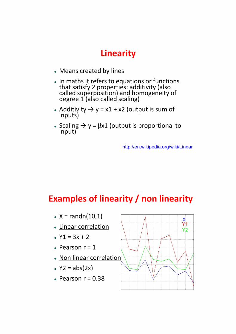
Examples of linearity / non linearity

X = randn(10,1)

Linear correlation

Y1 = 3x + 2

Pearson r = 1

Non linear correlation

Y2 = abs(2x)

Pearson r = 0.38

X Y1

Y2

06/04/2015

4

What is a linear model?

What is a linear model?

An equation or a set of equations that models data and which corresponds geometrically to straight lines, plans, hyperplans and satisfy the properties of additivity and scaling.

Simple regression: y = β1x1+ β2 + ε

Multiple regression: y = β1x1+ β2x2+ β3+ ε

One way ANOVA: y = µ + αi + ε

Repeated measure ANOVA: y= u + Si+ αi + ε

…

06/04/2015

5

A regression is a linear model

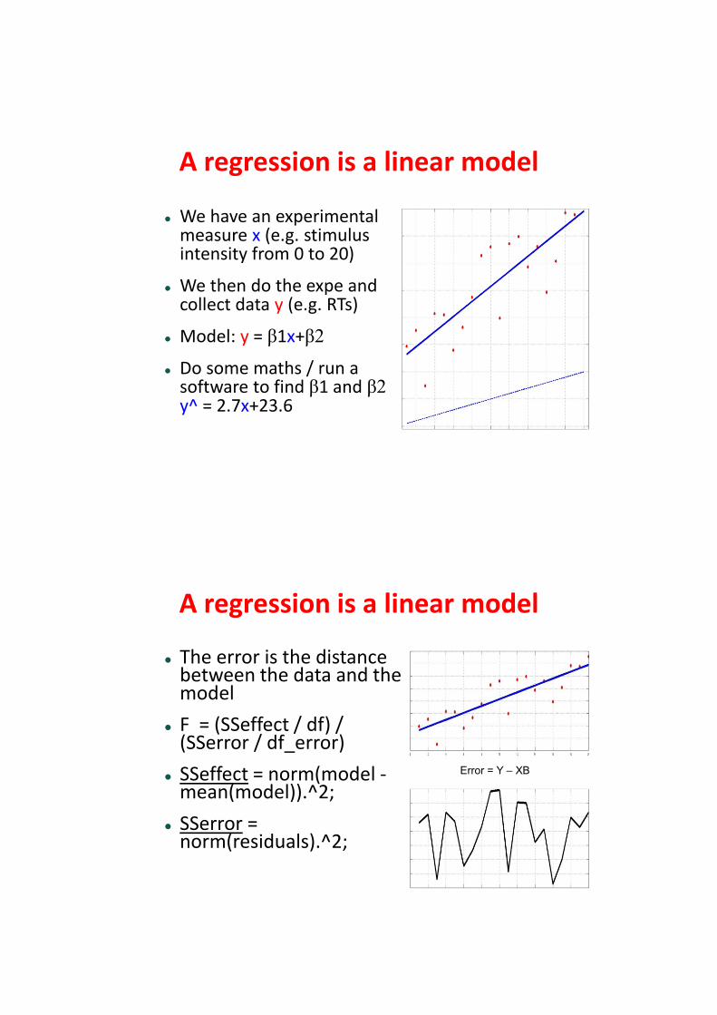
We have an experimental measure x (e.g. stimulus intensity from 0 to 20)

We then do the expe and collect data y (e.g. RTs)

Model: y = β1x+β2

Do some maths / run a software to find β1 and β2 y^ = 2.7x+23.6

A regression is a linear model

The error is the distance between the data and the model

F = (SSeffect / df) / (SSerror / df_error)

SSeffect = norm(model - mean(model)).^2;

SSerror = norm(residuals).^2;

Error = Y – XB

06/04/2015

6

Summary

Linear model: y = β1x1+ β2x2 (output = additivity and scaling of input)

A simple fMRI model

http://www.fil.ion.ucl.ac.uk/spm/data/auditory/

06/04/2015

7

FMRI experiment

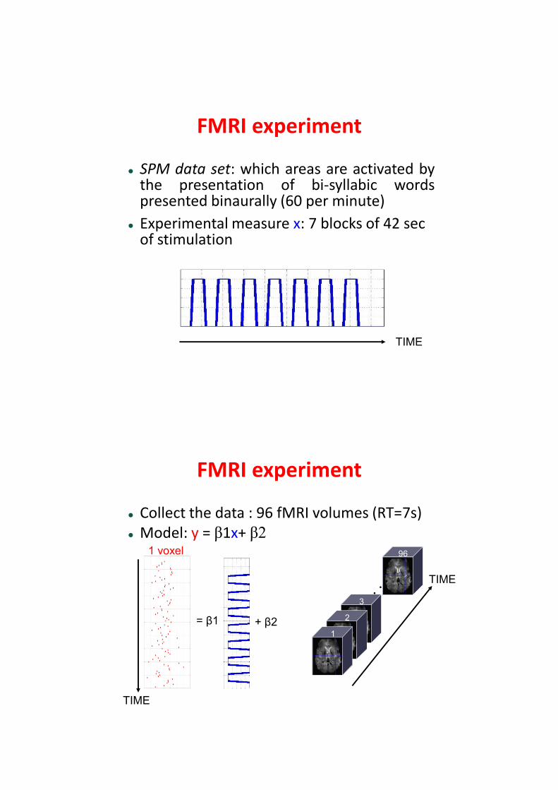
SPM data set: which areas are activated by the presentation of bi-syllabic words presented binaurally (60 per minute)

Experimental measure x: 7 blocks of 42 sec of stimulation

TIME

FMRI experiment

Collect the data : 96 fMRI volumes (RT=7s)‏ Model: y = β1x+ β2

96

1

2

3

TIME

1 voxel

β2‏+ β1‏=

TIME

06/04/2015

8

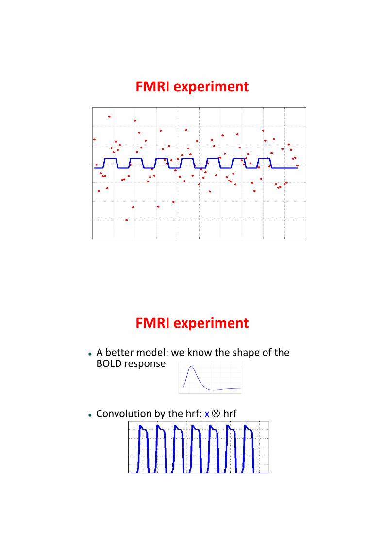
FMRI experiment

FMRI experiment

A better model: we know the shape of the BOLD response

Convolution by the hrf: x hrf

06/04/2015

9

FMRI experiment

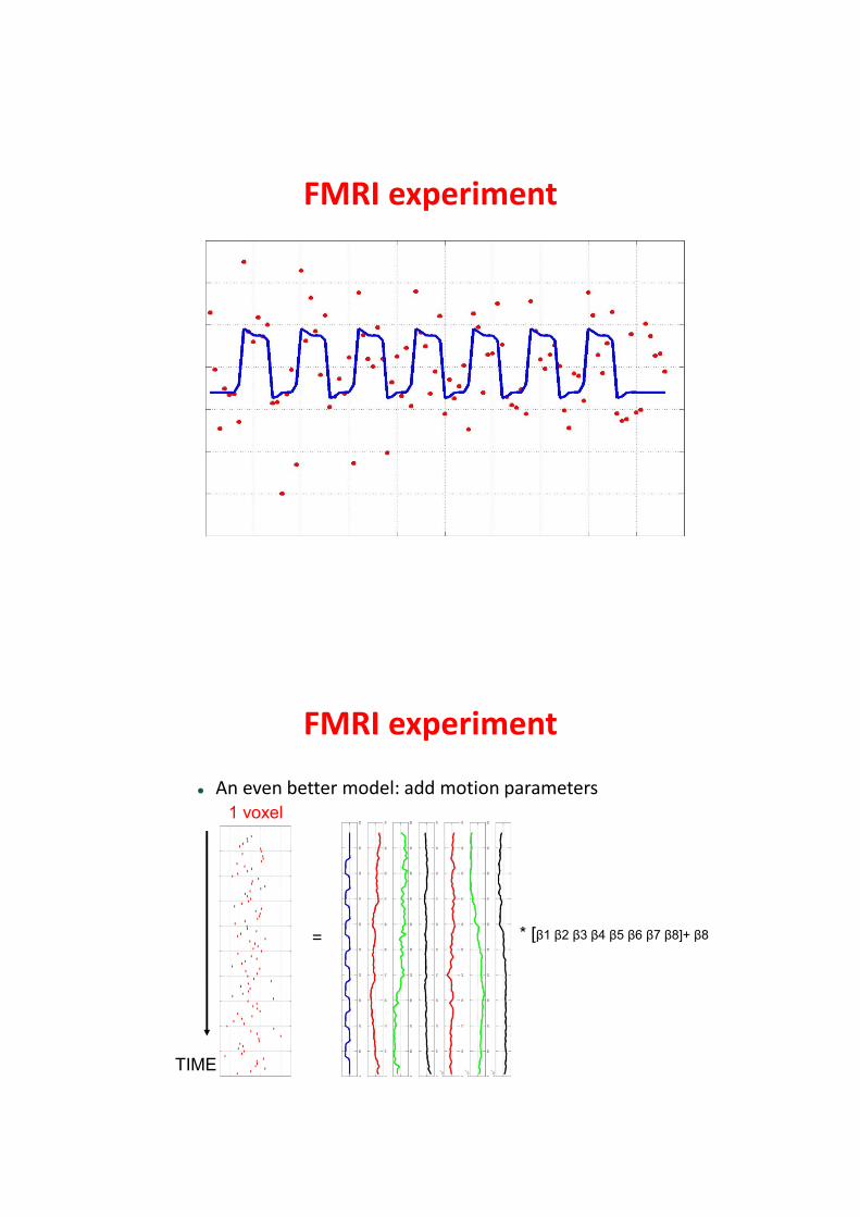
FMRI experiment

An even better model: add motion parameters

TIME

1 voxel

= * [β1 β2 β3 β4 β5 β6 β7 β8]+‏β8

06/04/2015

10

FMRI experiment

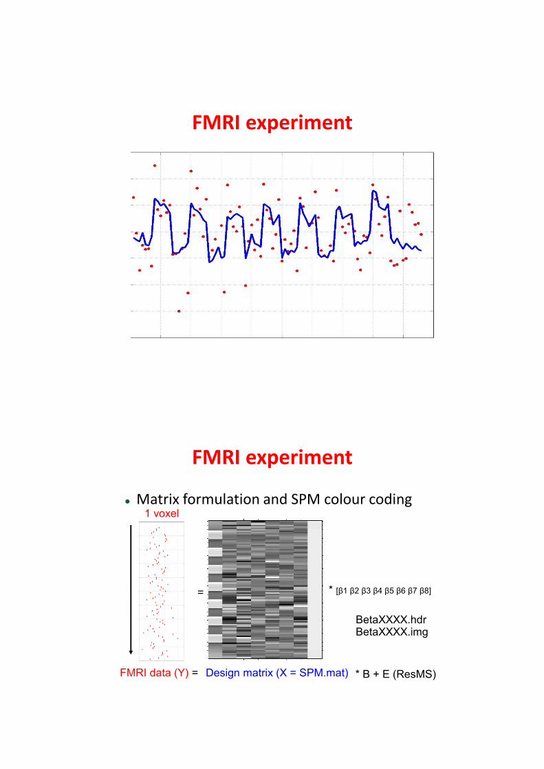
FMRI experiment

Matrix formulation and SPM colour coding

FMRI data (Y) =

1 voxel

= * [β1 β2 β3 β4 β5 β6 β7 β8]

Design matrix (X = SPM.mat)‏

BetaXXXX.hdr BetaXXXX.img

* B + E (ResMS)

06/04/2015

11

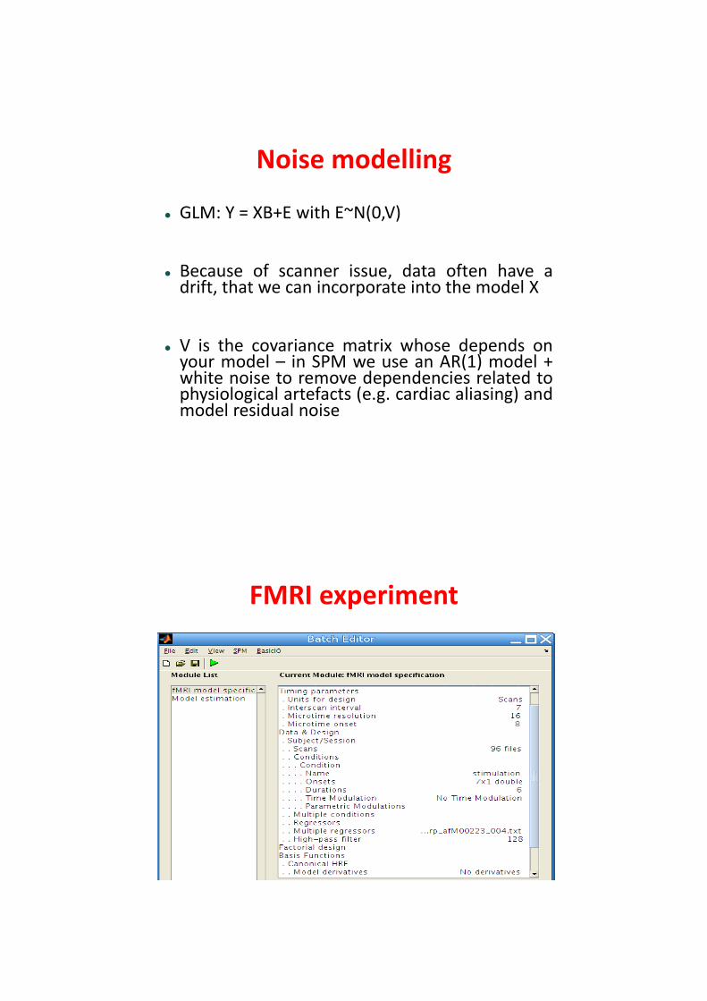
Noise modelling

GLM: Y = XB+E with E~N(0,V)

Because of scanner issue, data often have a drift, that we can incorporate into the model X

V is the covariance matrix whose depends on your model – in SPM we use an AR(1) model + white noise to remove dependencies related to physiological artefacts (e.g. cardiac aliasing) and model residual noise

FMRI experiment

06/04/2015

12

Summary

Linear model: y = β1x1+ β2x2 (output = additivity and scaling of input)

GLM: Y = XB+E (matrix formulation, works for any statistics, express the data Y as a function of the design matrix X)

Contrasts

06/04/2015

13

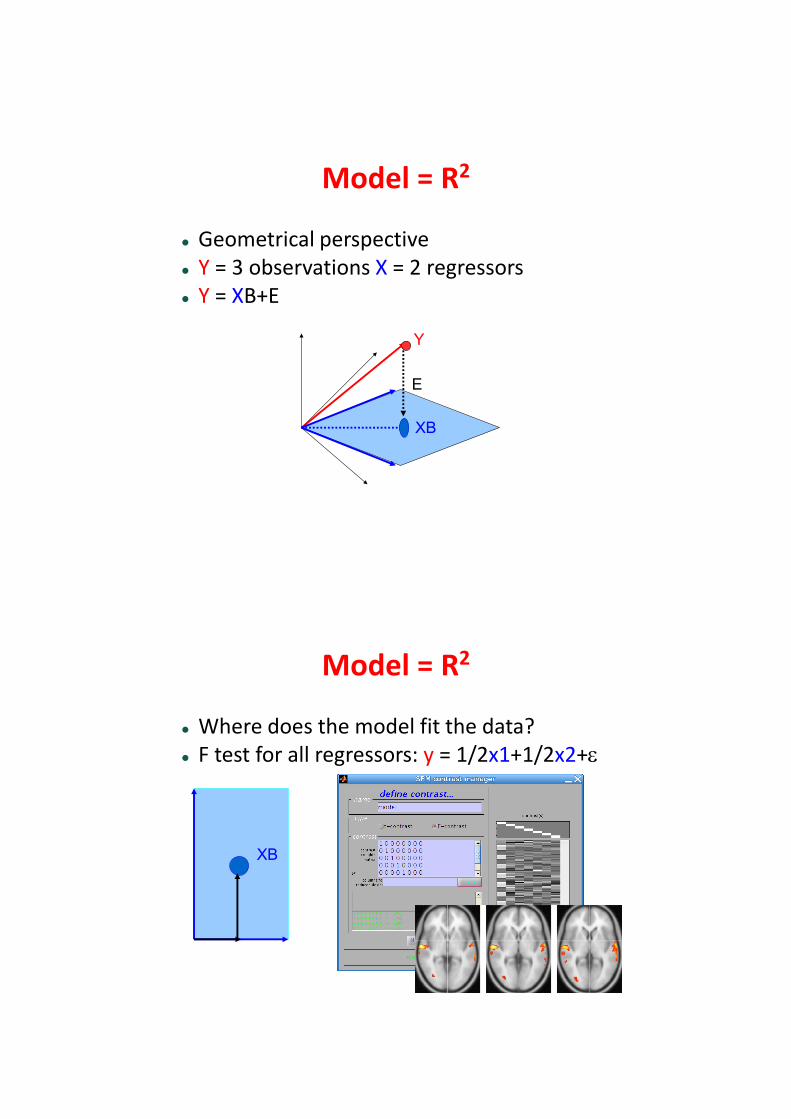
Model = R2

Geometrical perspective Y = 3 observations X = 2 regressors Y = XB+E

Y

XB

E

Model = R2

Where does the model fit the data? F test for all regressors: y = 1/2x1+1/2x2+

XB

06/04/2015

14

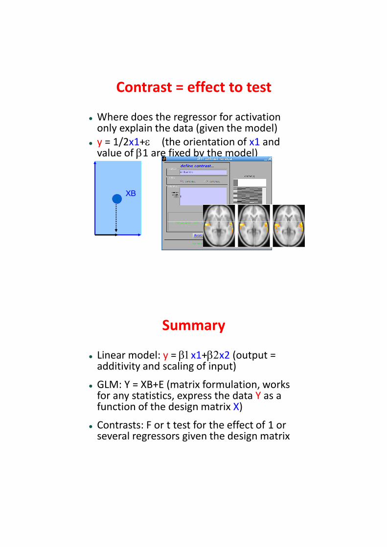
Contrast = effect to test

Where does the regressor for activation only explain the data (given the model)

y = 1/2x1+(the orientation of x1 and value of 1 are fixed by the model)

XB

Summary

Linear model: y = x1+x2 (output = additivity and scaling of input)

GLM: Y = XB+E (matrix formulation, works for any statistics, express the data Y as a function of the design matrix X)

Contrasts: F or t test for the effect of 1 or several regressors given the design matrix

06/04/2015

15

Issues with regressors

More contrasts

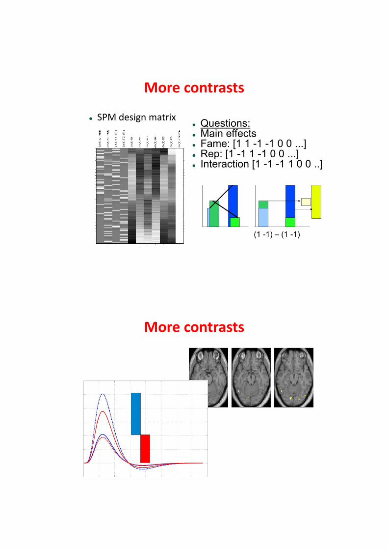
New experiment: (Famous vs. Nonfamous) x (1st vs 2nd presentation) of faces against baseline of chequerboard

2 presentations of 26 Famous and 26 Nonfamous Greyscale photographs, for 0.5s, randomly intermixed, for fame judgment task (one of two right finger key presses).

http://www.fil.ion.ucl.ac.uk/spm/data/face_rep/face_rep_SPM5.htm

06/04/2015

16

More contrasts

SPM design matrix Questions: Main effects Fame: [1 1 -1 -1 0 0 ...] Rep: [1 -1 1 -1 0 0 ...] Interaction [1 -1 -1 1 0 0 ..]

‏(1- 1) – ‏(1- 1)

More contrasts

06/04/2015

17

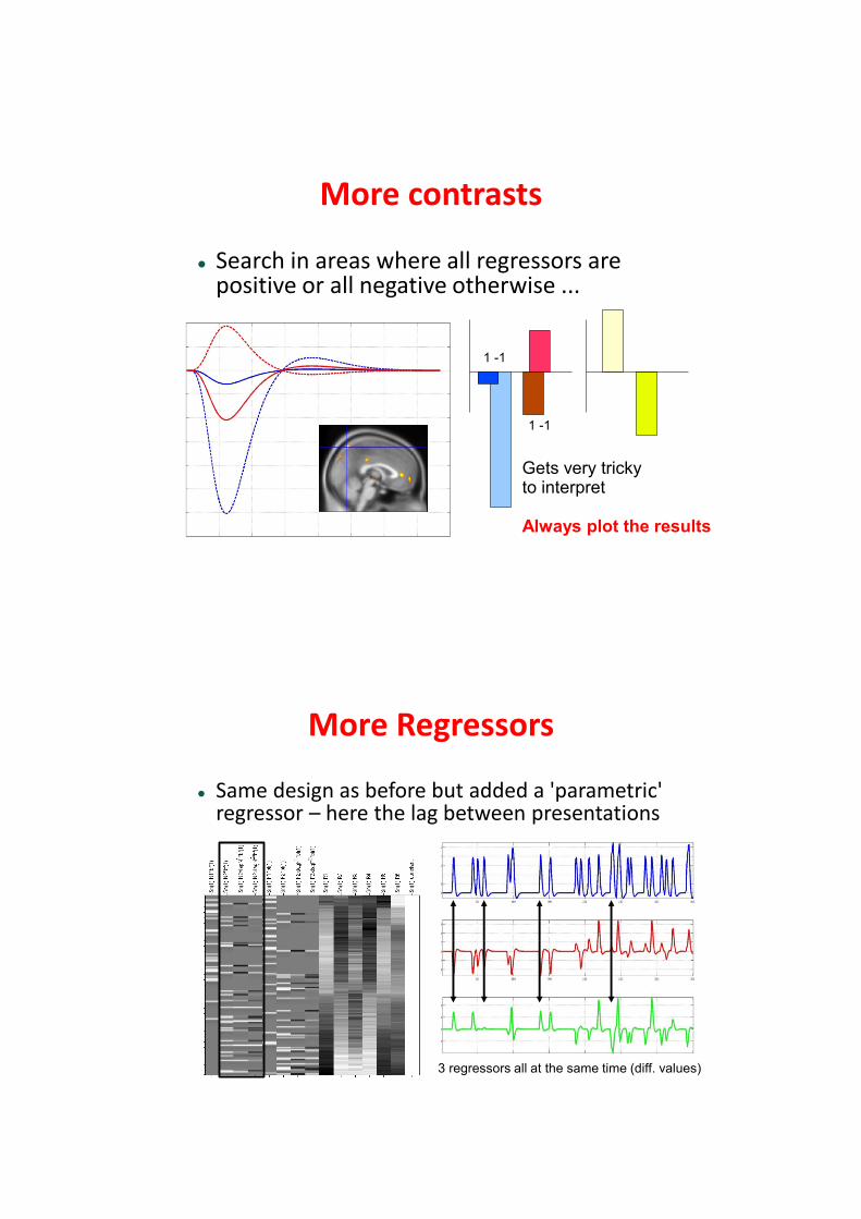
More contrasts

Search in areas where all regressors are positive or all negative otherwise ...

1 -1

1 -1

Gets very tricky to interpret Always plot the results

More Regressors

Same design as before but added a 'parametric' regressor – here the lag between presentations

3 regressors all at the same time (diff. values)‏

06/04/2015

18

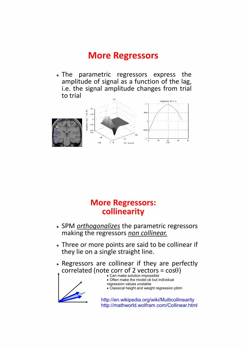
More Regressors

The parametric regressors express the amplitude of signal as a function of the lag, i.e. the signal amplitude changes from trial to trial

More Regressors: collinearity

SPM orthogonalizes the parametric regressors making the regressors non collinear.

Three or more points are said to be collinear if they lie on a single straight line.

Regressors are collinear if they are perfectly correlated (note corr of 2 vectors = cos)

http://en.wikipedia.org/wiki/Multicollinearity http://mathworld.wolfram.com/Collinear.html

Can make solution impossible Often make the model ok but individual regression values unstable Classical height and weight regression pblm

06/04/2015

19

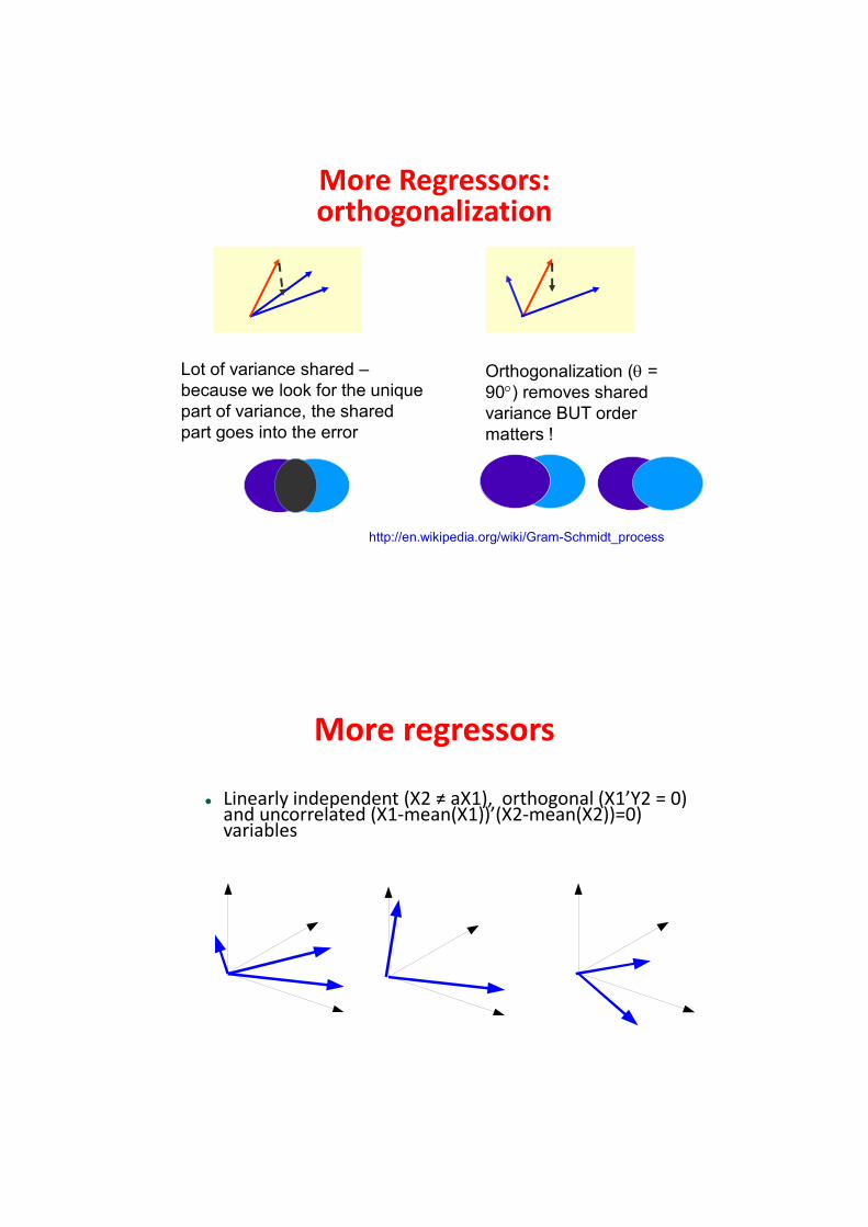
More Regressors: orthogonalization

Lot of variance shared –

because we look for the unique

part of variance, the shared

part goes into the error

Orthogonalization ( =

90) removes shared

variance BUT order

matters !

http://en.wikipedia.org/wiki/Gram-Schmidt_process

More regressors

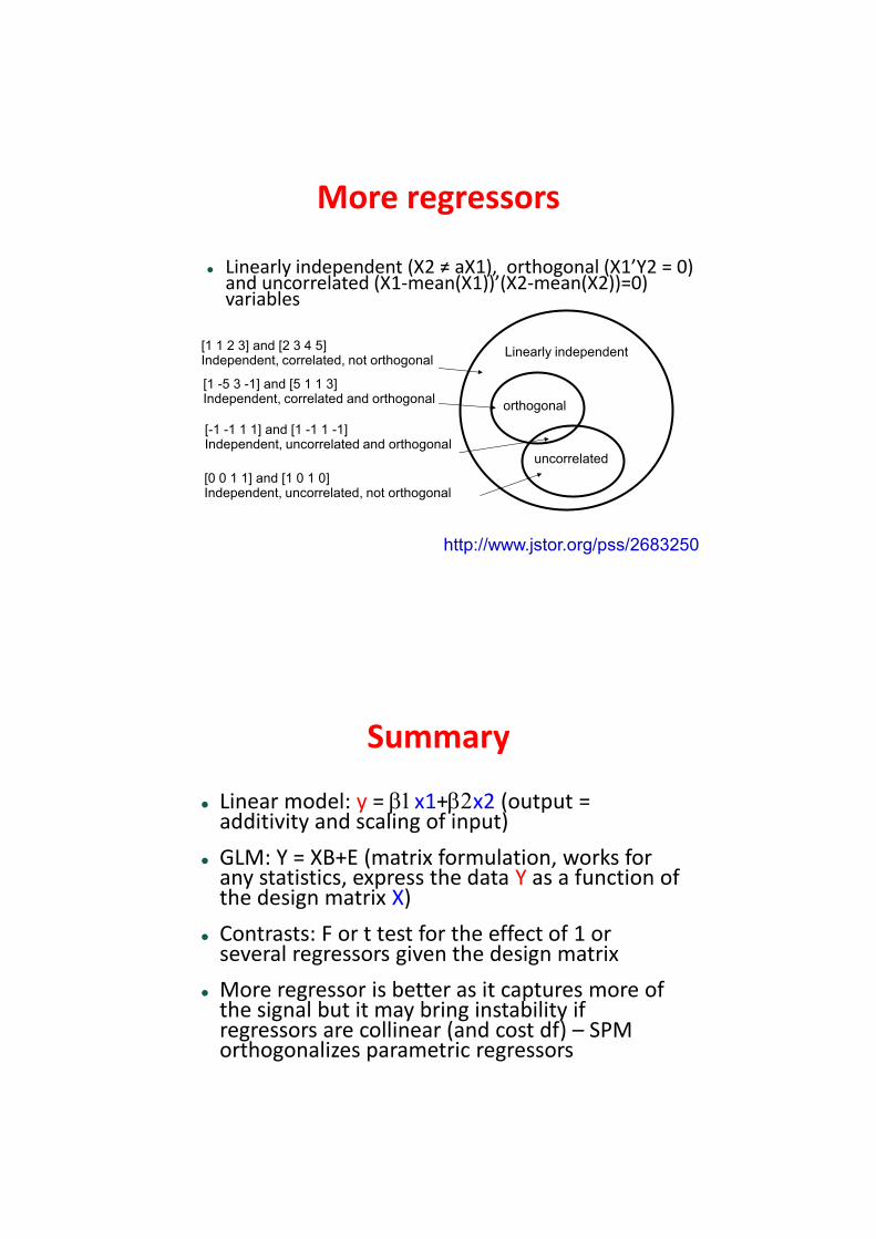
Linearly independent (X2 ≠ aX1), orthogonal (X1’Y2 = 0) and uncorrelated (X1-mean(X1))’(X2-mean(X2))=0) variables

06/04/2015

20

More regressors

Linearly independent (X2 ≠ aX1), orthogonal (X1’Y2 = 0) and uncorrelated (X1-mean(X1))’(X2-mean(X2))=0) variables

Linearly independent [1 1 2 3] and [2 3 4 5] Independent, correlated, not orthogonal

[1 -5 3 -1] and [5 1 1 3] Independent, correlated and orthogonal

orthogonal

uncorrelated

[-1 -1 1 1] and [1 -1 1 -1] Independent, uncorrelated and orthogonal

[0 0 1 1] and [1 0 1 0] Independent, uncorrelated, not orthogonal

http://www.jstor.org/pss/2683250

Summary

Linear model: y = x1+x2 (output = additivity and scaling of input)

GLM: Y = XB+E (matrix formulation, works for any statistics, express the data Y as a function of the design matrix X)

Contrasts: F or t test for the effect of 1 or several regressors given the design matrix

More regressor is better as it captures more of the signal but it may bring instability if regressors are collinear (and cost df) – SPM orthogonalizes parametric regressors