STOCK INDEX FUTURES MARKETS:STOCHASTIC VOLATILITY MODELS AND SMILES†

Robert G. TompkinsVisiting Professor, Department of Finance

Vienna University of Technology* andPermanent Visiting Professor, Department of Finance

Institute for Advanced Studies

† This piece of research was partially supported by the Austrian Science Foundation(FWF) under grant SFB#10 (Adaptive Information Systems and Modelling in Economicsand Management Science). This paper has benefited from comments by Stewart Hodges,Walter Schachermayer, Friedrich Hubalek, Stephan Pichler, Ole Barndorff-Nielsen, NeilShephard and attendees at the University of Aarhus mini-symposium on volatility and theAustrian Working Group on Banking and Finance. The author would also like to thank theeditor of this journal and the two referees for extremely helpful suggestions forimprovements. As always, I am responsible for all remaining errors.

* Böcklinstrasse 7/1/7, A-1020 Wien, Austria, Phone: +43-1-726-0919, Fax: +43-1-729-6753, Email: rtompkins@ins.at

1

STOCK INDEX FUTURES MARKETS:STOCHASTIC VOLATILITY MODELS AND SMILES

ABSTRACT

This paper examines whether the inclusion of an appropriate stochastic volatility that captureskey distributional and volatility facets of Stock Index Futures is sufficient to explain impliedvolatility smiles for options on these markets.

Two variants of stochastic volatility models related to the Heston (1993) are considered. Thesemodels are differentiated by alternative normal or non-normal processes driving log-priceincrements. For four stock index futures markets examined, models including a negativelycorrelated stochastic volatility process with non-normal price innovations perform best withinthe total sample period and for sub-periods.

Using these optimal stochastic volatility models, prices of European options are determined.Comparisons of simulated and actual options prices for these markets find substantialdifferences. This suggests that the inclusion of a stochastic volatility process consistent withthe objective process alone is insufficient to explain the existence of smiles.

JEL classifications: C15, G13

Keywords: Stochastic Volatility, Normal Inverse Gaussian Distributions, Methods ofMoments Estimation, Implied Volatility Smiles.

2

1. INTRODUCTION

Soon after the publication of the Black-Scholes (1973) paper on option pricing, Black

(1975) pointed out that the constant volatility assumption may be incorrect; noting that the

volatility may be a function of the underlying price level. Subsequent research has identified

the existence of different volatilities implied from option prices for different strike prices and

terms to maturity [see Jackwerth and Rubinstein (1996) for a review of this literature]. This

effect has been commonly referred to as the implied volatility smile (for options with the same

term to expiration) and the term structure of volatility (for options with different terms to

expiration).

Broadly speaking, two possible reasons have been proposed to explain these effects.

The first approach assumes that market imperfections exist that systematically prevent option

prices from taking their true Black-Scholes values. Such market imperfections include the

introduction of errors associated with discrete hedging, transactions costs, incomplete markets

and heterogeneous market agents with diverse expectations. Alternatively, a number of papers

have examined the implications for option prices when the underlying asset price process

differs from the lognormal diffusion process and/or the volatility is neither constant [as in

Black-Scholes (1973)] nor a deterministic function [as in Merton (1973)]. Mayhew (1995)

provides a brief review of both approaches. This research examines the latter hypothesis.

This paper examines the nature of the objective dispersion processes for stock index

futures and proposes the inclusion of stochastic volatility to explain these empirical facets of

the objective price processes. Once this is done, the implications for option pricing are

considered. Previous research has examined the effects of stochastic volatility (in the

underlying objective price process) on option pricing [see Johnson & Shanno (1987), Hull &

White (1987), Scott (1987), Wiggins (1987), Melino and Turnbull (1990), Stein & Stein

(1991) and Heston (1993)]. This paper extends this line of research.

3

The models considered include non-normality in the underlying log-price process and

correlated price and volatility processes. Due to the rich nature of these models, they do not

lend themselves to parameterisation using standard methods (such as maximum likelihood

methods) and a simulated method of moments approach was utilised. The choice of target

empirical moments was done to address most stylised results previously pointed out in the

literature. Specifically, higher moments of the return series were consided, as were dynamics

of the volatility process and leverage effects. Once suitable parameter values for alternative

models were found and a feasible risk-neutral drift adjustment was derived, options prices

were determined numerically assuming the drift adjustment was unique1.

To allow comparisons between the simulated and actual option prices, all prices were

re-expressed as standardised implied volatilities and plotted as surfaces. Substantial

differences between these surfaces were found for the S&P 500 futures market and this

suggests that the inclusion of stochastic volatility for the objective process alone is insufficient

to explain the existence of implied volatility smiles. However, consistent divergences between

simulated and actual implied volatility surfaces were found across for four markets and this

may provide insights into the nature of market imperfections and risk premia. Scott (1987)

completed similar research on stock options and found similar results. He suggested that

further research should test the effects of stochastic volatility on the pricing of options for a

larger sample. This paper achieves this by examination of four stock index futures and options

markets for a period encompassing the decade of the 1990s.

The paper is organised as follows: the first part briefly reviews previously presented

empirical evidence, which indicates that stock index futures prices do not follow an

independent and identically distributed (i.i.d.) Geometric Brownian Motion (GBM) process.

Two possible models, which have been proposed in the literature to explain these results, were

considered. Seven empirical attributes were selected to capture key aspects of non-normality

and inter-dependence. A description of the data sources used for this research follows. After

this, both possible models were examined using a simulated method of moments approach to

assess their ability to explain the key attributes. Having determined the best model, option

prices were estimated consistent with these processes and were then expressed as implied

volatilities using the Black (1976) formula. These simulated implied volatility surfaces were

compared to the implied volatility surfaces from traded options on the S&P 500 futures

markets. Finally, conclusions and suggestions for further research appear.

4

2. PRICE PROCESSES FOR STOCK INDEX FUTURES

UNDER THE 'EMPIRICAL' MEASURE

It is well established that the unconditional return series for individual stocks, stock indices

and Stock Index Futures do not conform to the assumptions of an i.i.d. lognormal dispersion

process [see Stoll & Whaley (1990)]. Returns for stock index futures usually display excess

kurtosis and (for many periods) significantly negative skewness compared to a normal

distribution. Returns for futures also display inter-temporal dependence. In the examination of

absolute returns for Stock Index markets, significant positive autocorrelations have been

found. This result has led Ding, Granger and Engle (1993) to conclude, "It is clear that the

S&P 500 stock market return process is not an i.i.d. process" (page 87).

Another line of empirical research has examined the unconditional volatility series

directly. A typical approach to better understand the volatility process is to examine the

statistical moments of the process. Burghardt and Lane (1990) examined the variability of the

unconditional volatility process using a volatility cone approach. We extended this by looking

at the sampling properties (restricted to the standard deviation) of the unconditional volatility

measured at a 20-day time horizon. Using non-overlapping data, we obtained an average

estimate of the unconditional volatility and the standard deviation of this average. Under the

assumption that an i.i.d. price process is generating these volatilities, the expected coefficient

of variation of the 20-day volatility is known. This measures the variability of volatility for a

given time horizon.

However, the time varying dynamics of the variability of volatility as the time

horizon of estimation is extended, is of additional interest. A simple log-linear form was

chosen to capture these dynamics. The rate of decay in the standard deviation of volatility

implies that the maturity structure of historical volatility experiences long-term memory

(interdependence). This can be seen as complimentary to long-term memory effects for

absolute returns identified by Ding, Granger and Engle (1993). An additional and important

feature of these price processes is the leverage effect pointed out by Christie (1982) among

others.

While a number of theories have been proposed to explain these results, three

alternative hypotheses will be examined here. The Constant Elasticity of Variance (CEV)

model of Cox and Ross (1976), a non-GBM price process model [such as the Jump diffusion

model proposed by Merton (1976)] and Stochastic Volatility Models were considered. These

5

three models can be nested within a stochastic volatility model. Given the wide range of

stochastic volatility models proposed in the literature [see Taylor (1994)], it was not obvious

which model to select. As models with correlated processes were considered, the Heston

(1993) model was the obvious choice. This model has the additional benefit of having a closed

form solution for the pricing of options [see Heston (1993), Bakshi, Cao and Chen (1997) and

Bates (2000)]. Variants of the Heston (1993) model proposed by Barndorff-Nielsen (1997) and

Barndorff-Nielsen and Shephard (1999) are also considered.

Specifically, the following three models were:

MODEL 1 )(tFdZFdtdF σµ += (1)

Where Z(t) is a standard Wiener Process and µ and σ are constants, the return series rt is

normally distributed with tt Zr σµ += and tZ ~ N(0,1). This is the assumption of the Black

(1976) model of i.i.d. Geometric Brownian Motion and will be referred to as GBM.

It is clear that Model 1 is a straw man, given the well-known results that Stock Index

futures returns display both non-normality and inter-dependence. However, this can serve as a

benchmark for the relative effectiveness of the alternative models and is used to assess the

sampling properties of the evaluation approach. Subsequent models will consider stochastic

volatility ( σ̂ ) which will be evaluated in terms of a stochastic variance process ( V ).

MODEL 2 1ˆFdZFdtdF σµ += (2.1)

With the variance process defined by:

2)( dZVdtVdV ξθκ +−= (2.2)

Where Z1 and Z2 are standard Wiener processes with correlation ρ. The term κ indicates the

rate of mean reversion of the variance, θ is the long-term variance and ξ indicates the volatility

of the variance. The terms V and √V represent the variance and the volatility of the process,

respectively. This model will be referred to as SV in this paper.

MODEL 3 Ν+= FdFdtdF σµ ˆ (3.1)

With the variance process defined by:

dZVdtVkdV ξθ +−= )( (3.2)

where Ν represents a non-normal price process for the underlying price series and in this

research is the Normal Inverse Gaussian distribution (NIG). This model is related to that of

6

Barndorff-Nielsen (1997) who was the first to propose a stochastic volatility model of this

form [subsequently extended by Andersson (1999a)]. This approach extends the findings of

Bates (1996, 2000) and Ho, Perraudin and Sørensen (1996), who assumed the volatility

process is subordinated in a non-normal price process. In this model, the stochastic variance

process is assumed to follow a standard Wiener Processes, Z, with correlation ρ existing

between the two processes.2 When correlated processes are considered, this variant of model 3

is related to the model for incorporating a leverage effect in a stochastic volatility model

proposed by Barndorff-Nielsen and Shephard (1999). This model will be referred to a NIGSV

in this paper. The CEV model of Cox and Ross (1976) which allows for the inclusion of

negative correlations between the two stochastic processes is nested in both Models 2 and 3.

This allows the leverage effect to be captured.

3. CHOICE OF ATTRIBUTES AND FITTING PARAMETER VALUES

A key problem in the empirical testing of stochastic volatility models is the estimation of

optimal input parameters into the model. Andersen, Chung and Sørensen (1999) provide a

good review of the approaches used to parameterise stochastic volatility models. Many of the

models considered here do not lend themselves to estimation by traditional maximum

likelihood methods. Andersen, Chung and Sørensen (1999) propose the use of the efficient

method of moments approach suggested by Gallant and Tauchen (1996). Their primary

contributions are to understand the sample properties of this estimator and show that the

method is robust in larger sample sizes. Recently, Andersson (1999b) also examined the

maximum likelihood estimator of the NIGSV model of Barndorff-Nielsen (1997) and by

Monte Carlo simulation demonstrated that a simulated method of moments approach is

equally robust. Due to the complexities of our models, it is not clear whether estimation of

parameter inputs by maximum likelihood techniques is feasible. Given that these papers have

demonstrated that parameter estimation via simulation can be equally robust and this approach

may provide a better intuitive understanding of the estimation procedure, a simulated method

of moments approach similar in spirit to General Method of Moments (GMM) was utilised.

This research uses a hybrid between the Generalised Method of Moments (GMM)

approach of Melino and Turnbull (1990) and the Simulated Method of Moments (SMM)

approach of Duffie and Singleton (1993). This approach subjectively selects essential

attributes, simulates price processes consistent with the alternative models and assesses the

sum of squared errors between simulated and empirical attributes. Alternative parameterisation

of the models was examined and optimised. Similar to Andersen, Chung and Sørensen (1999),

7

we investigated the sample properties of this estimator technique (using Model 1). This

allowed comparisons to be made between the attributes of each market and the models and

conclusions to be drawn regarding the overall fit of each model.

At the heart of this estimation technique is the judicious choice of key attributes. It is

crucial that the choice of the attributes jointly considers the relevant elements of empirical

interdependence and non-normality and provides a means by which the salient features of the

alternative models can be captured. Given that both alternative price process (to GBM) and

stochastic volatility models have been proposed to explain excess kurtosis in returns, the

unconditional kurtosis for daily returns is a logical attribute to choose. Furthermore, some

research has indicated that negative skewness is an important attribute for describing the

returns of stock indices and stock index futures. Both Theodossiou (1998) and Harvey and

Siddique (1998) chose to examine the skewness in addition to the excess kurtosis. This

attribute would provide evidence for the existence of asymmetric jumps and/or leverage

effects.

To examine both of these moments, price changes were estimated based upon

continuously compounded returns in the standard manner (using log-price increments).

Extreme care was taken to assure that returns were estimated using only futures prices with the

same expiration date. With this time series of daily returns, the unconditional skewness and

kurtosis statistics were determined.

Clearly, given that this research examined two variants of a stochastic volatility

model, attributes had to be selected that would allow the salient features of these models to be

captured. This required attributes capturing the volatility of volatility parameter, the rate of

mean reversion and the correlation between the processes. For this research, the estimation of

the standard deviation of the returns was determined using squared returns and these results

were annualised (assuming 252 trading days in a year). A number of attributes were selected

in order to capture critical dynamics of the volatility process.

The first attribute examines the volatility of volatility. A time series of unconditional

volatilities was estimated on a daily basis for a time horizon of 20 days (using non-overlapping

data). From this series, the average and standard deviation were estimated. Given widely

different levels of these sample statistics, a coefficient of variation statistic was chosen as the

key attribute. As a basis for comparison, the coefficient of variation of volatility measured at

8

the 20th lag would be approximately equal to 0.1622 if the underlying return series were

independent and identically distributed [1/√(2*19)].

While this measured the variability of volatility at a single time horizon, the time

varying dynamics of the standard deviation of volatility could not be captured. This was

achieved by the estimation of the coefficient of variation of volatility with time horizons from

20 days to 200 days in 20-day increments.3 From statistical theory, the expected decay in the

standard deviation of a volatility estimate ( *σ ) is a square root function of the number of

observations used for estimation ( NSE 2/*σ= ). Given that the average level of volatility

remains constant (which was found empirically for these four markets), the decay in the

coefficient of variation should follow the same functional form. If the first volatility

observation is at the 20-day horizon, the decay in the standard deviation of volatility from that

point forward can be expressed as 1+

⋅N

NNσ . In this formula, Nσ is the standard deviation of

the volatility at the Nth observation and N+1 is the number of observations in the next time

horizon (initially N=20 and N+1=40). The functional form of this decay can be expressed as a

power function of the form 5.0*

2−×= NSE σ . A linear regression of (the natural logarithms of) the

time horizon of estimation regressed upon the levels of the coefficient of variation was used to

capture the empirical rate in decay. This can be expressed as:

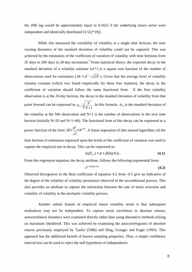
))(ln()ˆln( NN βασ += . (4.1)

From this regression equation, the decay attribute, follows the following exponential form:

))(ln( Ne βα + (4.2)

Observed divergences in the Beta coefficient of equation 4.2 from -0.5 give an indication of

the degree of the volatility of volatility persistence observed in the unconditional process. This

also provides an attribute to capture the interaction between the rate of mean reversion and

volatility of volatility in the stochastic volatility process.

Another salient feature of empirical return volatility series is that subsequent

realisations may not be independent. To capture serial correlation in absolute returns,

autocorrelation dynamics were examined directly rather than using alternative methods relying

on maximum likelihood. This was achieved by examining the autocorrelograms of absolute

returns previously employed by Taylor (1986) and Ding, Granger and Engle (1993). This

approach has the additional benefit of known sampling properties. Thus, a simple confidence

interval test can be used to reject the null hypothesis of independence.

9

For the purposes of this research, composite measures of the autocorrelations are

required. Given that the markets differ in the manner that the autocorrelations decay, the

averages of the autocorrelations from lag 1 to 20 and from lag 51 to 70 were both selected.

The first average represents the short-term autocorrelation. The medium-term average

provides an indication of how quickly the autocorrelations die out. Unfortunately, such

measures may no longer have known sampling properties allowing for a simple parametric

confidence interval test. Therefore, to assess the sample characteristics of these composite

measures, nonparametric confidence intervals were determined via simulation. These two

attributes provide additional information relevant to the calibration of a stochastic volatility

model, as they capture both short-term and medium-term evidence of volatility clustering.

The final attribute must measure the leverage effect and provide a means for a

correlation between the stochastic processes to be captured. There is, however, one problem

with the determination of the leverage effect: Even if the volatility is a stationary series, the

prices are not. To solve this problem, a new variable was constructed which measures recent

price movements and is stationary.4 This variable is an exponentially weighted return series,

which indicates whether recent price movements are relatively high or low. It can be shown

that given some exponential weighting scheme: where θ−=1W and tWe ∆−≈θ , we can define

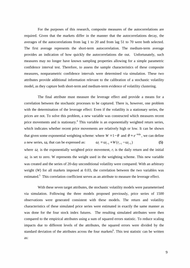
a new series, ωi, that can be expressed as: )( 111 −−− −+= iiii rW ωωω (5)

where iω is the exponentially weighted price movement, ri is the daily return and the initial

iω is set to zero. W represents the weight used in the weighting scheme. This new variable

was created and the series of 20-day unconditional volatility were compared. With an arbitrary

weight (W) for all markets imposed at 0.03, the correlation between the two variables was

estimated.5 This correlation coefficient serves as an attribute to measure the leverage effect.

With these seven target attributes, the stochastic volatility models were parameterised

via simulation. Following the three models proposed previously, price series of 1500

observations were generated consistent with these models. The return and volatility

characteristics of these simulated price series were estimated in exactly the same manner as

was done for the four stock index futures. The resulting simulated attributes were then

compared to the empirical attributes using a sum of squared errors statistic. To reduce scaling

impacts due to different levels of the attributes, the squared errors were divided by the

standard deviation of the attributes across the four markets6. This test statistic can be written

as:

10

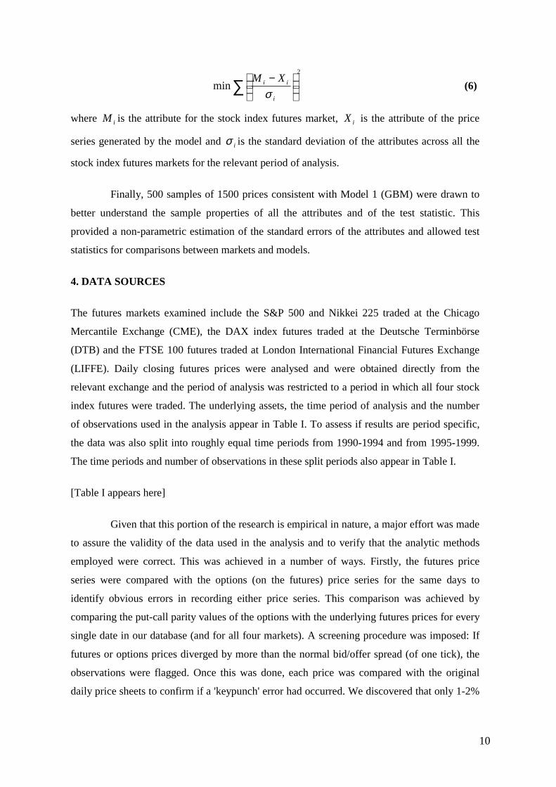
2

min∑

−

i

ii XMσ

(6)

where iM is the attribute for the stock index futures market, iX is the attribute of the price

series generated by the model and iσ is the standard deviation of the attributes across all the

stock index futures markets for the relevant period of analysis.

Finally, 500 samples of 1500 prices consistent with Model 1 (GBM) were drawn to

better understand the sample properties of all the attributes and of the test statistic. This

provided a non-parametric estimation of the standard errors of the attributes and allowed test

statistics for comparisons between markets and models.

4. DATA SOURCES

The futures markets examined include the S&P 500 and Nikkei 225 traded at the Chicago

Mercantile Exchange (CME), the DAX index futures traded at the Deutsche Terminbörse

(DTB) and the FTSE 100 futures traded at London International Financial Futures Exchange

(LIFFE). Daily closing futures prices were analysed and were obtained directly from the

relevant exchange and the period of analysis was restricted to a period in which all four stock

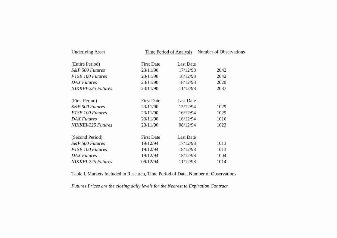
index futures were traded. The underlying assets, the time period of analysis and the number

of observations used in the analysis appear in Table I. To assess if results are period specific,

the data was also split into roughly equal time periods from 1990-1994 and from 1995-1999.

The time periods and number of observations in these split periods also appear in Table I.

[Table I appears here]

Given that this portion of the research is empirical in nature, a major effort was made

to assure the validity of the data used in the analysis and to verify that the analytic methods

employed were correct. This was achieved in a number of ways. Firstly, the futures price

series were compared with the options (on the futures) price series for the same days to

identify obvious errors in recording either price series. This comparison was achieved by

comparing the put-call parity values of the options with the underlying futures prices for every

single date in our database (and for all four markets). A screening procedure was imposed: If

futures or options prices diverged by more than the normal bid/offer spread (of one tick), the

observations were flagged. Once this was done, each price was compared with the original

daily price sheets to confirm if a 'keypunch' error had occurred. We discovered that only 1-2%

11

of the data had such errors. Nevertheless, these errors were of a sufficient magnitude that they

did influence the results and therefore required correction.

The most arduous of the data cleaning process was the ongoing examination of the

data as results of the analysis were obtained. One reason why four stock index futures and

options markets were examined was to allow a cross-sectional comparison. Apart from the

benefit of assessing general tendencies across markets, it is also possible to use anomalous

results as an additional check on data validity. This assured that the data series employed in

this research was as accurate as is humanly possible.

5. ATTRIBUTES FOR INDIVIDUAL MARKETS

For each market, the return statistics for daily returns were determined for the entire period of

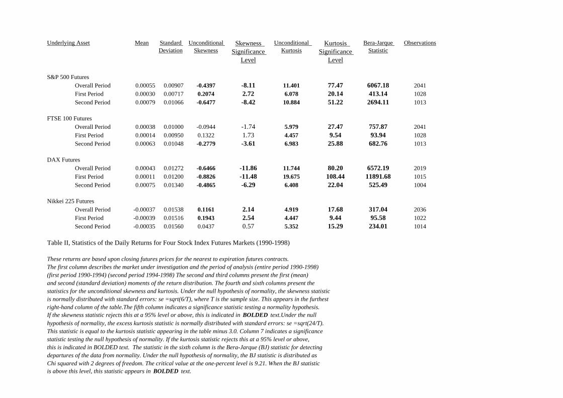
analysis and for each sub-period. The results of these analyses can be seen in Table II.

[Table II appears here]

The first column describes the market under investigation and indicates the time

period examined. The second and third columns present the mean and standard deviation of

the return distribution. The fourth and fifth columns present the statistics for the unconditional

skewness and these provide a significance level relative to a null hypothesis of normality.7 All

skewness significance statistics that are significantly different from the normal assumption at a

95% level (±1.96) appear in bold type. In the sixth and seventh columns, the unconditional

kurtosis statistic and the significance level relative to a null hypothesis of normality appear.8

When this statistic does not reject the null hypothesis of normality at the 95% level or above,

the statistic and the significance levels are in bolded type. The statistic in the eighth column is

the Bera-Jarque (BJ) statistic for detecting departures of the data from normality. Under the

null hypothesis of normality, the BJ statistic is distributed as χ2 with 2 degrees of freedom.

The critical value at the one-percent level is 9.21. When the BJ statistic exceeds this level, this

statistic also appears in bolded type.

For all four markets, the dispersion of returns is not well described by a normal

distribution. For many of the four markets, the skewness statistic tends to be significantly

different than that of a normal distribution. However, the skewness is neither consistently

negative for all markets nor always significant. On the other hand, for all four markets (and for

all time periods), the daily returns always display significant excess kurtosis. These two

12

factors lead to all BJ values exceeding their critical values. These results are consistent with

previous empirical examination of return series for stock markets by Theodossiou (1998) and

Harvey & Siddique (1998).

As the remaining attributes all capture characteristics of the volatility process, these

will be summarised in a single table, Table III.

[Table III appears here]

In this table, the first column describes the individual market examined and the time

period of the analysis. The next three columns display the average annualised volatility

measured at a 20-day time horizon. At the bottom of these columns are the expected attributes

from a GBM dispersion process with constant variance. The attribute of interest to this

research is the Coefficient of Variation statistic. For all four markets and for all time periods,

we can compare this measure of the volatility of volatility to what would be expected under

the GBM assumption. By determining a standard error of this attribute by simulation, we can

reject the hypothesis that the volatility process conforms to the GBM i.i.d. assumption.

In the fifth column appears the beta of the regression of the relationship between the

[natural logarithms of the] time horizon of the estimation period against the coefficient of

variation of volatility. If markets conform to a GBM i.i.d. process, a decay coefficient of -.50

(seen at the bottom of the column) would be observed. For each market, the rate of decay is

(statistically) significantly less that this decay function (the standard error of this attribute is

estimated in a non-parametric manner by simulation). In Column six, the leverage correlation

coefficient appears. This measures the relationship between the 20-day unconditional volatility

and the recent relative prices. Consistent with the negative leverage effects Christie (1982)

pointed out for individual stocks, stock index futures markets also seem to have a significant

negative leverage effect. The exceptions are the FTSE 100 and S&P 500 Futures over the first

period (1990-1994). These results should be interpreted with care given that the simulated

standard error of this attribute is fairly high (at 0.0999). While these effects remain significant,

it is only (barely) at the 95% level.

The final two columns represent the average autocorrelations of absolute returns for

lagged periods from 1-20 days and 51-70 days. Underlying the assumption of an i.i.d. price

process, these have a prior expectation of zero. For all four markets and for all time periods,

these averaged autocorrelations are statistically significantly positive. However, the degree of

autocorrelations seems to be higher in the second period relative to the first period.

13

The results from both tables II and III indicate that both the return series and the

volatility process are significantly divergent from a prior assumption of a GBM i.i.d. process.

With these attributes as target conditions, the proposed alternative models were examined.

6. FITTING ALTERNATIVE MODELS

In previous sections the models to be tested were presented. It only remains to discuss

technical issues in the simulation process and the parameterisation of the stochastic volatility

models before proceeding directly to the results.

The simulated method of moment’s approach was done in a two-stage process. The

first stage was to determine representative distributions for the later simulations. Specifically,

this entailed the generation of 500 samples of 1500 draws from an independent normal

distribution. According to standard procedures, the random number generation process used a

standard Box-Muller method and the anti-thetic approach suggested by Boyle (1977). With

these 500 samples, price series were constructed that conformed to GBM with constant

variance (using equation 1). The distributional and time series attributes of each series were

assessed and compared to the theoretical moments of an i.i.d. GBM process. Utilising formula

6, the sum of squared errors between each of the 500 samples and the true attributes of an i.i.d.

GBM process were determined. The two distributions with the lowest sums of squared errors

relative to the priors were selected as representative normal distributions. For the sake of

convenience, the normal disturbances for the underlying price process will be referred to as Z1

and the normal disturbances for the volatility process will be referred to as Z2. These two

series were uncorrelated. Thereafter, whenever simulation used either of these distributional

forms, the same sets of random numbers were used (to reduce errors introduced by the

selection of random numbers). Table IV details the results of the simulated GBM price series

and provides the sample standard deviation of the 500 simulated series.

[Table IV appears here]

In this table, the theoretical attribute values for a GBM process are listed as are the

average attribute values and the standard deviations of the attributes across the 500

simulations. Of crucial interest are the sampling properties of the attributes and especially the

sum of squared errors (SSE) statistic. The standard deviation of this statistic was found to be

equal to 4.5646 and will be used subsequently as a means to establish confidence intervals for

14

the comparison of the alternative models. Finally, the characteristics of the two representative

draws of the GBM process appear in the bottom two rows.

To generate the NIG distributions, random numbers were generated using the method

suggested by Rydberg (1997). These simulations required the input of the four moments of the

distribution. The first moment (mean) was set to 0.0 and the second moment (variance) to 1.0.

The third (skew) and fourth (excess kurtosis) moments were chosen to be less than the

observed moments for daily returns in Table III. This was done, due to the fact that the

stochastic volatility will interact with the NIG distribution and yield simulated moments that

are amplified compared to the NIG moments. Given these effects could not be ascertained

prior to the simulation, four NIG distributions were simulated and all were examined as

potential candidates for the underlying price process. These four possible NIG distributions

appear in Table V as NIG#1 to NIG#4.

[Table V appears here]

This approach contains an apparent inconsistency: while the random numbers

estimated conform to a NIG distribution, prices were simulated assuming that a risk-neutrality

condition exists. When the underlying price process follows an alternative process, such as a

NIG distribution, a correction to the drift term is required to allow risk neutral evaluation. An

appropriate risk-neutral drift adjustment is:

tt

ta t

tt ∆⋅

−

−−∆⋅+−∗

∆= −

−1222

122 )(

σµβασβαδ

(7)

Where at is the risk neutral adjusted drift, the Greek letters, α, β, δ, and µ are the parameters

of the NIG distribution and σt-1 is the random volatility (from stochastic volatility process in

equation 3.2) for the previous discrete observation. A complete proof of the derivation of this

drift adjustment appears in Appendix 1.9 This drift is then used in equation 3.1 with the drift

term (µ) equal to at-1 from equation 7 and the disturbances are drawn from the NIG

distribution.

Finally, to simulate correlated processes, we estimated a new set of random numbers

(Z') for the volatility process using the usual method for drawing samples from a standardised

bivariate distribution: 22 )1( ZZ ⋅−+⋅Ζ=′ ρρ (8)

Where Ζ represents the random disturbances for the underlying price process (in the case of

GBM, the Z1 set of normal draws, in the case of a NIG process, the draws from one of the four

15

samples). The term, Z2, refers to the representative normal distribution selected for the

volatility process and the term, ρ, refers to the correlation coefficient between the two

processes.

Once the distributions were drawn, the second stage of the simulated method of

moment’s approach was done in three steps. The first step was to simulate price and volatility

series that were consistent with the proposed models and secondly, determine the attribute

values for this simulated series. The third step entailed varying the paramater inputs into the

models to minimise the sum of squared errors relative to the observed empirical attributes. To

efficiently perform the third step, a starting point was to examine the sensitivities of the

overall sum of squared errors to a small incremental change in each of the parameter inputs

(holding the other parameters constant). Of the four variables in both of the stochastic

volatility models, it was found that only three of the factors were critical. For a given long-

term volatility, θ (taken as the average 20-day volatility in Table III), the crucial factors are the

rate of mean reversion, κ, the volatility of the volatility, ξ and the correlation between the

price and volatility process, ρ. It was found that small changes in the level of the long-term

volatility had almost no effect on the sum of squared errors. Given that only three parameters

needed to be varied, the parameterisation simply compared the sum of the squared errors using

the initial seeded parameter values to the sum of squared errors for the same model (and

random numbers) but varying the three critical parameters (κ,ξ and ρ). By varying only three

parameters both up and down, thus, only eight alternatives to the original results had to be

compared. If one of the new combinations of parameters achieved a lower sum of squared

errors, this model would replace the previous model. The search routine continued to search

the "cube" of eight adjacent alternative parameter combinations until no new combination

yielded better results. The initial search procedure first used fairly high increments in the

adjacent corner search (for example 1.0 for κ and 0.1 for ξ and ρ). When optimal parameters

were found, the increments for the search was progressively reduced (for example, as low as

0.01 for κ and 0.0001 for ξ and ρ) until no further reduction in the sum of squared errors was

achieved. When no further improvement in the sum of squared errors is possible, the final

combination of parameter values is deemed the optimal estimation of the alternative stochastic

volatility models.

Tables VIa, VIb, VIc and VId display the empirical attributes (taken from Tables II

and III) and the results of the models for each of the stock index futures markets. These results

are split into the three periods of analysis. In each of these tables, the three time periods of

16

analysis appear. On the left-hand side, the parameterisation of each of the three models

appears. Only the parameter values and the NIG distribution that has the lowest SSE are

presented. On the right-hand side, the simulated attributes of each model appear with the

empirical attributes directly above for comparison's sake. In the column immediately to the

right of this the sum of squared errors (SSE) for each model appears. The final column

indicates a T-test statistic comparing models 2 and 3 to the GBM assumption. This is

computed by taking the difference in the SSE for the models compared to the GBM case and

dividing this by the simulated standard error of the SSE statistic found in Table IV.

[Tables VIa, VIb, VIc and VId appear here]

As was expected, the GBM model with constant variance is rejected in favour of

models 2 and 3. The T-statistics indicate a rejection at well above a 99% confidence interval.

If we assume that the model with the lowest SSE is optimal, of twelve data sets, Model 3

(NIGSV) is the best in nine and Model 2 (SV) is the best for the remaining three. For all

twelve data sets, correlated processes were indicated.

These comparisons provide insights into which attributes are addressed by the facets

of the proposed models. The pure stochastic volatility model (SV) addresses the volatility

clustering effects measured by the two autocorrelation attributes as well as other volatility

dynamics [the volatility of volatility (CoV attribute) and the decay of this over time (Line fit)].

The inclusion of correlated processes allows the leverage effect and the negative skewness in

the returns to be captured. However, this model still fails to generate sufficient excess kurtosis.

Model 3 (NIGSV) is able to capture all seven attributes.

Comparisons between Models 2 and 3 can be made by examination of the T-test

statistics in Tables VIa to VId. As the T-test statistics provide an indication of the

improvement in these models relative to the GBM case, taking the differences between these

statistics provides insights into marginal improvement of Model 3 to Model 2. In nine of the

twelve cases, Model 3 has a higher T-statistic. However, the differences are small. For all

attributes except the excess kurtosis, both models perform equally well. What appears to be

most critical is the inclusion of correlations between the underlying price and volatility

processes. These capture the leverage and a portion of the skewness effect.

17

7. IMPLICATIONS FOR OPTION PRICING

From the preceding section, a more realistic price process for the four stock index futures

markets has thus been uncovered. This will serve as a prior process for the estimation of

option values. The next step is to examine the implications for options based upon these assets.

Given that the parameter estimation of the stochastic volatility models relies upon simulation,

it is a simple matter to use a similar simulation technique to estimate option prices. This

simulation approach determines European call and put options numerically (a Monte Carlo

approach) over a variety of strike prices and times to expiration. This is similar in spirit to the

approach used by Johnson and Shanno (1987).

In the immediately preceding section, it was demonstrated that in almost all instances

Model 3 (NIGSV) was optimal, therefore, only this was considered for the estimation of

option values.10 The choice of the appropriate input parameters for this model is taken from

the previous section and is based on the results for the entire period of analysis.

An apparent inconsistency for this approach is that the use of Monte Carlo

simulations to price options assumes that a risk-neutrality condition exist. This suggests that

the state space is continuous and spanned across that space by existing securities. However,

for the model examined, stochastic volatility, correlated processes and (negative) jumps have

been introduced into the state space. Given that no securities exist allowing the state space to

be spanned when the volatility displays such dynamics, these models do not permit us (in the

strictest sense) to use the risk-neutrality argument to price the options. This is an apparent

theoretical inconsistency. However, the determination of the risk-neutral drift adjustment for

the NIGSV process in equation 7 does allow limited comparisons of the simulated options

prices to be made actual option prices, which are evaluated under the risk neutral measure.

While, the equivalent risk-neutral measure in equation 7 is certainly feasible, it may not be

unique. This research examines whether this measure is unique by first assuming that both

simulated and actual option prices are evaluated under an equivalent risk-neutral measure. If

this is case, we can assess if this alternative price process alone is sufficient to explain the

existence of implied volatility smiles. If this is not the case, this may suggest that the

equivalent risk-neutral measure is not unique and markets are incomplete.

In this simulation, price series of three months in length were determined. Given that

the estimation of the unconditional (historical) dispersion processes was completed for trading

days, options were also priced using trading time instead of calendar time. The assumed

18

number of trading days in a year is 252. Option prices were estimated at time horizons from

one week (five trading days) to three months (in 5-day increments). Such options would

correspond to typical terms to maturity of actively traded options on Stock Index Futures.

To gain a better understanding of the impacts of the alternative models across strike

prices, fifteen strike prices were examined. The median strike price was centred at the starting

value of the simulation and was equal to 100. As the assumed underlying assets were futures

or forward contracts, the interest rate was assumed to zero. This corresponds to an at-the-

money option relative to the forward price.

The impacts of the model on options with different strike prices were of additional

interest. The analysis was restricted solely to out-of-the-money strike prices. Thus, when the

strike price was equal to or below the starting value of 100, the option evaluated was an

European put and when the strike price was above 100, the option evaluated was an European

call. A non-trivial problem is the choice of strike prices so that as maturities of options vary,

meaningful comparisons can be drawn. In previous papers on the impacts of stochastic

volatility on option prices, strike price determination has taken one of two forms. Authors

have either chosen to fix a single maturity and vary the strike prices in terms of "moneyness"

[see Hull & White (1988)] or fixed the degree of moneyness (or strike prices) and examined

the impacts across different maturities [see Henker and Kazemi (1998)].

Unfortunately, both methods do not allow meaningful conclusions to be drawn

regarding the impacts of the models on option prices across time and a consistent measure of

moneyness. Natenberg (1994) and Tompkins (1997) have proposed a more consistent measure

of strike price. This was slightly modified to: 252/

)/ln(τσ

ττ FX (9)

where X is the strike price of the option, F is the underlying futures price and the square root

of time factor reflects the percentage in a trading year of the remaining time until the

expiration of the option. The sigma (σ) is the at-the-money volatility.

This adjustment notes that the distance of an option strike price to the level of the

underlying asset is relative, both in respect to the current price of the underlying, the time to

expiration and the level of expected volatility. This adjustment converts all strike prices into a

metric that can be interpreted as a standard deviation. Thus, in this analysis, strike price ranges

± 3.5 standard deviations away from the at-the-money level in 0.5 standard deviation

increments were examined. This change in measure will allow more direct comparison of

19

model impacts on option prices where the time to maturity varies but the relative strike prices

remain the same. 11

For the simulations, the volatility parameter chosen was equal to the level of

volatility used in the parameter determination of all models for each of the four markets for the

entire period of analysis. Given the extremely wide range of volatilities across the four

markets, the standardisation of the strike prices allows direct comparisons to be made and

allows subsequent comparisons to be made with actual implied volatility surfaces.

For the Monte Carlo simulation, random numbers consistent with a GBM process

were determined using a Box-Muller technique and employed the anti-thetic approach

suggested by Boyle (1977) for both. This series was later used to determine the bivariate

distribution used to estimate the stochastic volatilities. This series of random numbers were

stored and used for all subsequent estimations of stochastic volatility. For each of the three

NIG distributions, 10000 were drawn using the method suggested by Rydberg (1997). The

same approach was used for the estimation of the optimal stochastic volatility parameters in

the previous section. These were also stored and used for all analysis using that particular NIG

distribution. Then, the bivariate distribution was estimated for the volatility series using

formula 7 and the optimal parameters of Model 3 for each stock index futures in Tables VIa,

VIb, VIc, and VId (for the entire period of analysis).

With the appropriate NIG distribution and the estimated bivariate distribution for the

stochastic volatility, volatilities and prices were estimated using an Euler approach (discrete

form of formula 3.1 and 3.2). With the prices of each model estimated, the payoffs of the

fifteen options (at each point in time) were determined and the result averaged. As interest

rates were assumed to be zero, there is no need to discount the result to present value.

In parallel, we estimated the prices of all the options for each market using the Black

(1976) model with the same strike prices as the simulation, the same term to expiration and the

volatility equal to the same long-term volatility used in the simulations. The underlying futures

prices used in the determination of the Black (1976) price were equal to the average futures

price in the simulation at the same point in time. Given that the underlying asset is a futures

contract, the interest rate and dividend yield was set to zero (the same assumptions were made

when estimating the Model 3 option prices).

Although, standardisation of the strike prices simplifies comparisons between the

four markets, the sheer amount of information makes such comparisons cumbersome. Thus,

20

only the results for a single market, the S&P 500, are presented. Furthermore, to simplify

comparisons between simulated and actual implied volatility surfaces; the simulated option

prices were expressed as implied volatilities. These implied volatilities were further

standardised by indexing them to the constant volatility assumed in the Black (1976) model

(dividing each of the implied volatilities by the assumed constant volatility and multiplying by

100). The indexed implied volatilities are then presented as a continuous surface relative to the

standardised strike prices and time to expiration. This surface for the S&P 500 futures appears

in the middle panel of Figure 1 and is titled: Simulated Implied Volatility Surface. This figure

has been scaled to allow direct comparison to actual implied volatility surfaces of options on

the S&P 500 futures (which appears in the upper panel).

[Figure 1 appears here]

The simulated implied volatility surface for the S&P 500 appears to display some of

the features reported by Derman & Kani (1994), and Corrado & Su (1996). The characteristic

curvature of volatility smiles is found and there is some degree of negative skewness

(especially for longer maturity options). While we have not explicitly discussed the impacts of

this model across a cross-section of option prices, this figure implicitly displays these impacts.

For all the markets, the Black (1976) pricing model overvalues options that are at-the-money

and within a significant range around (and above) the at-the-money level. The shaded areas

below 100 represent this in the graphs. For out-of-the-money options, the Black (1976) model

tends to undervalue option prices (especially for options with lower strike prices) and the

overpricing bias tends to increase the longer the term to expiration. These results are consistent

with the biases of stochastic volatility on option prices found elsewhere [Hull & White

(1988)]. Similar results are found for the other three stock index futures markets

In the top panel of Figure 1, the actual implied volatility surface associated with

options on S&P 500 futures appears. To construct this surface, implied volatilities were

estimated using the Black (1976) model for all (out of the money) options on the S&P 500

futures. The period of analysis was from November 1990 to December 1998

(contemporaneous with the period of analysis of the S&P 500 Futures). Analysis was

restricted solely to options with the same terms to expiration as were used for the simulated

option prices (5 days to 3 months in 5-day increments) and excluded all options prices

allowing arbitrage [see Jackwerth & Rubinstein (1996)]. The strike prices were then

converted to the same standardised form as was done for the simulated implied volatility

surfaces (using formula 9) and the levels of implied volatility were indexed to the level of the

21

at-the-money implied volatility. Then, the indexed implied volatilities were grouped by the

same term to expiration. Finally, for each term to expiration, a polynomial fitting procedure

[see Shimko (1993) and Tompkins (1999)] was implemented to yield an implied volatility

smile. These were then combined and the volatility surface was drawn.12

For the actual implied volatility surface associated with options on the S&P 500, it is

clear that the degree of curvature is most extreme when the options are closest to expiration

and becomes more linear with longer expirations. For the simulated surfaces, the effect is the

opposite. Furthermore, the implied volatility surfaces for the actual options market are much

more curved that for the simulated surfaces.

Another important difference is that the actual implied volatility surface displays

much greater asymmetry than the simulated surface. Options with strike prices below the

current futures price have higher implied volatilities than options with higher strike prices.

Similar results are found for the other three markets.

These differences are a consequence of the model chosen under the objective

measure. Let us consider each facet of the NIGSV model separately. The NIG process for

returns captures the effects of non-normality in daily returns. Therefore, if subsequent

disturbances are independent, this process will rapidly approach that of a normal distribution

from the Central Limit Theorem. If the higher moments of the chosen NIG process were

sufficiently extreme, a more curved (and skewed) shape would be observed for options with

short terms to expiration; becoming more linear as the time horizon of the option were

extended. In the instance of S&P 500 futures, the optimal NIG price process for the S&P 500

(NIG #1) was insufficiently non-normal to produce the biases found with actual smiles. One

interpretation of this result is that the higher moments from the risk-neutral process are

different (more extreme) than those for the (risk-neutral adjusted) objective process.

The positive relationship between the degree of curvature in the simulated implied

volatility surfaces and the time to expiration is most probably due to the inclusion of the

stochastic volatility process. As was pointed out by Hull & White (1988), the degree of bias in

option pricing increases with the time to expiration of the option. This would produce an

implied volatility surface that would display more curvature the longer the term to expiration.

As the volatility process in equation 3.2 assumes a Gauss-Wiener process, this effect should be

symmetrical. However, the simulated surface displays an asymmetry relationship with the time

to expiration. This asymmetry is due to effects of the negative correlation between the

22

processes. Clearly, the longer the period, the greater the impact of the negative correlation.

Similar results are found for the other three stock index options markets.

The divergence between the patterns of implied volatility surfaces suggests that the

inclusion of our proposed stochastic volatility models in option pricing is insufficient to

explain the existence of implied volatility smiles. The most obvious conclusion is that we have

the wrong model and that some alternative approach may better describe the unconditional

price process for the underlying futures. However, it is unclear what the alternative approaches

would be. The models tested here included non-normality in the return process, stochastic

volatility and correlated processes. Most models proposed in the literature to explain the

objective price and volatility processes are nested in the model examined here.

A second possibility is that models we have examined are correct, but that our

method of parameter estimation has yielded incorrect model inputs. The potential problems

with parameter estimation could be due either to inadequacies of the simulated method of

moments approach or the selection of inappropriate (or incomplete) target moments. As the

former has been extensively examined in the literature and dismissed, this is unlikely. The

choice of target moments was determined including all relevant facets of non-normality and

volatility that have been pointed out in the empirical literature; it is unclear what additional

attributes would be included.

The third possibility is even if the price process of the underlying asset was correctly

modelled, it is not obvious that option prices would conform to this process. The Cox & Ross

(1976) link between the objective and risk-neutral processes would be incomplete in the

presence of non-traded sources of risk. For the models examined here, the introduction into

the state space of non-constant volatility, jump-processes and correlations between the two

processes would introduce just such non-traded sources of risk. Thus, it is clear that our

assumption of a unique martingale measure is incorrect. Given this is the case, a logical next

step would be to better understand the nature of this risk. Scott (1987) explicitly examined the

dynamics of the risk premium when volatility is stochastic and is not a traded security. We

will examine the nature of the risk premium implicitly by examination of the differences in the

simulated and actual implied volatility surfaces.

The simple difference between these two surfaces appears in the bottom panel of

Figure 1. Standardisation of both surfaces simplifies interpretation: as the percentage

difference in the (standardised) level of implied volatility. The actual implied volatilities are

23

between 10% and 70% higher than those associated with the implied volatilities consistent

with the objective price process. For the shortest to expiration options, almost none of the

curvature in the actual implied volatility surface is explained by model of the objective

process. Even so, the divergences between the surfaces are relatively symmetrical relative to

the ATM level for options with a short time period to expiration (out to 15 days to expiration).

One possible interpretation of this is that the skew effect for options on stock index futures

with short time periods to expiration might be due primarily to an alternative price process (a

NIG process with negative skewness). For longer terms to expiration, approximately one half

of the curvature in the actual implied volatility surface is addressed by the objective price

process model. However, for longer dated options the divergence in the surfaces is

asymmetric. The inclusion of correlated processes should address this. Even so (and using an

appropriate measure of the objective leverage effect), this appears insufficient to completely

explain this effect. For options with higher strike prices and a longer term to expiration (35

days to 90 days), the divergence between the two surfaces is small. However, the fact that

everywhere the difference between the surfaces is positive could be interpreted as evidence for

the existence of a risk premia. Alternatively this difference could be associated with

transaction costs or could be caused by other sources of market imperfections or frictions. For

the other three stock index futures markets, the differences in the simulated and actual implied

volatility surfaces display similar patterns. With the exception that for two of the other

markets, the divergence seems relatively time invariant (Nikkei and FTSE 100 Futures).

8. SUMMARY AND SUGGESTIONS FOR FUTURE RESEARCH

This paper examines the nature of the objective dispersion processes, which can be observed

for futures contracts on four stock indices. To capture the multi-faceted non-normality and

inter-dependence of the empirical dispersion processes, seven attributes were identified. With

these attributes for each of the four markets, two alternative stochastic volatility models were

examined. It was found that all four markets are best understood with a model which assumes

the price process follows a Normal Inverse Gaussian process and the stochastic process

driving volatilities is negatively correlated to this NIG process.

Based upon an optimal parameterisation of this model, European options were

determined numerically for each market. Significant divergences from the Black (1976) values

were observed. For all markets, this option pricing model tended to increase the prices of

options with lower strike prices relative to Black (1976) prices and decrease the value of ATM

and higher strike price options. This research points out for the first time the relative biases

24

associated with the option pricing model proposed by Barndorff-Nielsen and Shephard (1999).

This extends the research of Hull & White (1988) to consider a richer class of stochastic

volatility models.

Option prices consistent with the model were then expressed as standardised implied

volatility surfaces and compared to actual implied volatility surfaces from options on the S&P

500. While the simulated implied volatility surfaces display some stylised facts similar to

actual surfaces, differences are observed that are similar across all four markets. For the entire

surfaces, the actual option prices have higher implied volatilities than for option prices

consistent with the model. Therefore, we reject the hypothesis that the stochastic volatility

models proposed are sufficient to explain the existence of implied volatility smiles. Of interest

is that the differences between the implied volatility surfaces consistent with the objective and

risk-neutral processes appear to display similar dynamics for all four markets. The nature of

this difference should provide a useful starting point for future research into the nature of the

risk premium in options prices and provide insights into the relationship between the objective

and risk-neutral processes.

25

REFERENCES:

Andersen, T.G., Chung, H-J & Sørensen, B.E.(1999). Efficient method of moments estimationof a stochastic volatility model: A Monte Carlo study. Journal of Econometrics, 91, 61-87.

Andersson, J. (1999a). On the normal inverse Gaussian stochastic volatility model. Essays onFinancial Time Series Models, Stochastic Volatility and Long Memory, Acta UniversitatisUpsaliensis. Comprehensive Summaries of Uppsala Dissertations from the Faculty of SocialSciences, 82, 1-10.

Andersson, J. (1999b). Maximum Likelihood estimation of the normal inverse Gaussianstochastic volatility model. Comprehensive Summaries of Uppsala Dissertations from theFaculty of Social Sciences, 82. 1-11.

Barndorff-Nielsen, O.E. (1997). Normal Inverse Gaussian Distributions and StochasticVolatility Modelling. Scandinavian Journal of Statistics, 24, 1-13.

Barndorff-Nielsen, O.E. & N. Shephard (1999). Incorporation of a Leverage Effect in aStochastic Volatility Model. Working Paper, University of Aarhus.

Bates, D.S. (1996). Jumps and Stochastic Volatility: Exchange Rate Process Implicit in PHLXForeign Currency Options. Review of Financial Studies, 9, 69-107.

Bates, D.S. (2000). Post-'87 Crash Fears in the S&P 500 Futures Options Markets. Journal ofEconometrics, 94, 181-238.

Black, F. & Scholes, M. (1973). The Pricing of Options and Corporate Liabilities. Journal ofPolitical Economy, 81, 637-654.

Black, F. (1975). Fact and Fantasy in the Use of Options. Financial Analysts Journal, 31, 36-41,61-72.

Black, F. (1976). The Pricing of Commodity Contracts. Journal of Financial Economics, 3,167-179.

Burghardt,G. & Lane, M. (1990). How to Tell if Options are Cheap. Journal of PortfolioManagement, 16, 72-78.

Boyle, P.P.. (1977). Options: A Monte Carlo Approach. Journal of Financial Economics, 4,323-338.

Bakshi, G., Cao, C. & Chen, Z. (1997). Empirical Performance of Alternative Option PricingModels. Journal of Finance, 52, 2003-2049.

Christie, A.A., (1982). The Stochastic Behaviour of Common Stock Variances. Journal ofFinancial Economics, 10, 407-432.

Corrado, C.J. & Su, T. (1996). Skewness and kurtosis in S&P 500 Index returns implied byoption prices. Journal of Financial Research, 19, 175-192.

Cox, J.C. & Ross, C.A. (1976). The Valuation of Options for Alternative Stochastic Processes.Journal of Financial Economics, 3, 145-166.

26

Derman, E. & Kani, I. (1994). Riding on the Smile. RISK, 7 (2). 32-39.

Ding, Z., Granger, C.W.J. & Engle, R.F. (1993). A long memory property of stock returns anda new model. Journal of Empirical Finance, 1, 83-106.

Duffie, D., & Singleton, K.J. (1993). Simulated moments estimation of Markov models ofasset prices. Econometrica, 50, 929-952.

Gallant, A.R. & Tauchen, G. (1996). Which Moments to Match?. Econometric Theory, 12,657-681.

Garman, M. & Klass, M. (1980). On the Estimation of Security Price Volatilities fromHistorical Data. Journal of Business, 53, 67-78.

Harvey, C.R. & Siddique, A. (1998). Conditional Skewness in Asset Pricing Tests. WorkingPaper (June 4, 1998 version). Duke University, Durham North Carolina.

Henker, T. & Kazemi, H.B. (1998). The Impact of Deviations from Random Walk inSecurity Prices on Option Prices. Working Paper University of Massachusetts, Amherst.

Heston, S.L. (1993). A Closed-Form Solution for Options with Stochastic Volatility withApplications to Bond and Currency Options. Review of Financial Studies, 6, 327-343.

Ho, M.S., Perraudin, W.R.M. & Sørensen, B.E. (1996). A Continuous-Time Arbitrage-PricingModel with Stochastic Volatility and Jumps. Journal of Business & Economic Statistics, 14,31-43.

Hodges, S. & Tompkins, R. (2000). The Sampling Properties of Volatility Cones, FORC Pre-print 00/103, Financial Options Research Centre, University of Warwick.

Hull, J. & White, A. (1987). Hedging the Risks from Writing Foreign Currency Options. Journalof International Money and Finance, 6, 131-152.

Hull, J. & White, A. (1988). An Analysis of the Bias in Option Pricing Caused by a StochasticVolatility. Advances in Futures and Options Research, 3, 29-61.

Jackwerth, J.C. & Rubinstein, M. (1996). Recovering Probability Distributions from OptionPrices. The Journal of Finance, 51, 1611-1631.

Johnson, H. & Shanno, D. (1987). Option Pricing When the Variance is Changing. Journal ofFinancial and Quantitative Analysis 22, 143-152.

Mayhew, S. (1995). Implied Volatility. Financial Analysts Journal, 51 (4), 8-20.

Melino, A., & Turnbull, S.M. (1990). Pricing foreign currency options with stochasticvolatility. Journal of Econometrics, 45, 239-265.

Merton, R. (1973). The Theory of Rational Option Pricing. Bell Journal of Economics, 4, 141-183.

Merton, R. (1976). Options pricing when Underlying Stock Returns are Discontinuous.Journal of Financial Economics, 3, 125-144.

27

Natenberg, S. (1994). Option Volatility and Pricing: Advanced Trading Strategies andTechniques, Chicago, Illinois: Probus Publishing Company.

Parkinson, M. (1980). The Extreme Value Method for Estimating the Variance of the Rate ofReturn. Journal of Business, 53, 61-66.

Rydberg, T.H. (1997). The Normal Inverse Gaussian Lévy Process: Simulation andApproximation. Commun. Stat., Stochastic Models, 13, 887-910.

Scott, L.O. (1987). Option Pricing when the Variance Changes Randomly: Theory, Estimationand an Application. Journal of Financial and Quantitative Analysis, 22, 419-438.

Shimko, D. (1993). Bounds of Probability, RISK, 6, Number 4, 33-37.

Stein, E.M. & Stein, J.C. (1991) Stock Price Distributions with Stochastic Volatility: AnAnalytic Approach,” Review of Financial Studies, 4, 727-752.

Stoll, H.R. & Whaley, R.E. (1990). The Dynamics of Stock Index and Stock Index FuturesReturns. Journal of Financial and Quantitative Analysis, 25, 441-468.

Taylor, S.J. (1986). Modelling Financial Time Series, New York: John Wiley & Sons.

Taylor, S.J. (1994). Modelling Stochastic Volatility: A Review and Comparative Study.Mathematical Finance, 4, 183-204.

Theodossiou, P. (1998). Financial Data and The Skewed Generalized T Distribution.forthcoming in Management Science.

Tompkins, R.G. (1997). Measuring Equity Volatilities. in Equity Derivatives, London,England, RISK Publications.

Tompkins, R.G. (1999). Implied Volatility Surfaces: Uncovering Regularities for Options ofFinancial Futures. FORC Pre-print 98/93, Financial Options Research Centre, University ofWarwick, Coventry, England.

Wiggins, J.B. (1987). Option Values Under Stochastic Volatility: Theory and EmpiricalEstimates. Journal of Financial Economics, 19, 351-372.

28

FOOTNOTES:

1 A number of previous papers have made similar assumptions. Scott (1987), Hull & White (1987), andJohnson and Shanno (1987) either assumed the market price of volatility risk was zero or the existence of amarketable asset perfectly correlated to volatility.2 Barndorff-Nielsen (1997) actually assumed that the underlying price process follows GBM and the volatilityprocess follows an Inverse Gaussian distribution. However, it can be shown that this is equivalent to theunderlying price process following a NIG distribution and the volatility process follows GBM.3 The estimation of the volatilities was done using overlapping data. This introduces a bias in the estimation ofthe standard deviation of volatility. This bias was corrected using the Hodges and Tompkins (2000) approach.4 The author would like to thank Stewart Hodges (University of Warwick) for suggested the use of this variable.5 To simplify the selection of the attribute, a fixed weight of 0.03 was applied to all markets and for all periodsof analysis, to allow the leverage correlation factor to not be subject to differing weights. This was found to beclose to the optimal weights for each market using a maximum likelihood estimation procedure.6 In addition, the natural logarithm of the unconditional kurtosis was examined rather than the absolute levels.This was done due to wide variations in this statistic across the four markets. However, all results are presentedas absolute levels.7 Under the null hypothesis of normality, the skewness statistic is asymptotically normally distributed withstandard errors: se =√(6/T), where T is the sample size.8 Under the null hypothesis of normality, the excess kurtosis statistic is asymptotically normally distributed withstandard errors: se =√(24/T), where T is the sample size. This statistic is equal to the kurtosis statistic appearingin the table minus 3.0.9 In Appendix 1, it is noted there that this is only one manner to adjust this drift to achieve risk-neutrality.Given that this model implies markets are incomplete, there may not exist a unique martingale measure.However, this is certainly a feasible adjustment and will allow relative comparisons to be drawn.10 While for three of the twelve data sets, the SV model was marginally superior to the NIGSV model, thisdifference was found statistically significant.11 This manner of expressing the strike price is similar to the d2 term that appears in the Black Scholes formula.It is common market practice in the currency options market to express strike prices in terms of the delta[N(d2)] and quote implied volatilities relative to this. This approximately expresses equation 1 as a probability.12 Tompkins (1999) used a model expanding Shimko (1993) to include higher moments and time/strike priceinteractions. When implied volatility surfaces were standardised (relative to the ATM volatility). This modelwas able to explain 95% of the variance in the implied volatility surface of the S&P 500 and Tompkins (1999)demonstrated that this degree of explanatory power is retained outside of sample.

i

APPENDIX 1

Derivation of the Risk Neutral Drift Adjustment for aNormal Inverse Gaussian Process.

The process S, generated by the NIG distribution should be a martingale. In the discrete time setting thismeans:

[ ]11

|−−

=ℑjjj ttt SSE , j = 1,2,3,…,n 1.1

with 1−

ℑjt denoting the information at time tj-1. Since both the drift term, a, and the volatility, σ, are known at

time tj-1 , and the variance of the series Vj is independent from the history leading up until tj-1, this is equivalentto:

( ) ,11

1 =∆−

− ∆ tmej

jt

tta σ 1.2

where m(x) = E[exVj] is the moment generating function of the NIG(µ,δ,α,β) distribution.

This function is:

)))((exp()( 2222 xxxm µβαβαδ ++−−−= 1.3

So the appropriate choice of drift is:

( )

∆∆=

−

− tmta

j

j

tt

1

1

1ln1σ

1.4

Combining equations 1.3 and 1.4 leads to

tt

ta t

tt ∆⋅

−

−−∆⋅+−∗

∆= −

−1222

122 )(

σµβασβαδ

1.5

As a final note, adjusting the drift is only one way to obtain a martingale (for risk-neutral valuation). Given themodels examining suggest an incomplete market, there are alternative approaches. For example, for theconstant volatility NIG process in continuous time, the natural approach would be to estimate the parameters,µ,δ,α andβ from the observations of S and adjust β to obtain a risk neutral valuation.

Underlying Asset Number of Observations

(Entire Period) First Date Last DateS&P 500 Futures 23/11/90 17/12/98 2042FTSE 100 Futures 23/11/90 18/12/98 2042DAX Futures 23/11/90 18/12/98 2020NIKKEI-225 Futures 23/11/90 11/12/98 2037

(First Period) First Date Last DateS&P 500 Futures 23/11/90 15/12/94 1029FTSE 100 Futures 23/11/90 16/12/94 1029DAX Futures 23/11/90 16/12/94 1016NIKKEI-225 Futures 23/11/90 08/12/94 1023

(Second Period) First Date Last DateS&P 500 Futures 19/12/94 17/12/98 1013FTSE 100 Futures 19/12/94 18/12/98 1013DAX Futures 19/12/94 18/12/98 1004NIKKEI-225 Futures 09/12/94 11/12/98 1014

Table I, Markets Included in Research, Time Period of Data, Number of Observations

Futures Prices are the closing daily levels for the Nearest to Expiration Contract

Time Period of Analysis

Mean Standard Deviation

Unconditional Skewness

Skewness Significance

Level

Unconditional Kurtosis

Kurtosis Significance

Level

Bera-Jarque Statistic

Observations

S&P 500 FuturesOverall Period 0.00055 0.00907 -0.4397 -8.11 11.401 77.47 6067.18 2041First Period 0.00030 0.00717 0.2074 2.72 6.078 20.14 413.14 1028Second Period 0.00079 0.01066 -0.6477 -8.42 10.884 51.22 2694.11 1013

FTSE 100 FuturesOverall Period 0.00038 0.01000 -0.0944 -1.74 5.979 27.47 757.87 2041First Period 0.00014 0.00950 0.1322 1.73 4.457 9.54 93.94 1028Second Period 0.00063 0.01048 -0.2779 -3.61 6.983 25.88 682.76 1013

DAX FuturesOverall Period 0.00043 0.01272 -0.6466 -11.86 11.744 80.20 6572.19 2019First Period 0.00011 0.01200 -0.8826 -11.48 19.675 108.44 11891.68 1015Second Period 0.00075 0.01340 -0.4865 -6.29 6.408 22.04 525.49 1004

Nikkei 225 FuturesOverall Period -0.00037 0.01538 0.1161 2.14 4.919 17.68 317.04 2036First Period -0.00039 0.01516 0.1943 2.54 4.447 9.44 95.58 1022Second Period -0.00035 0.01560 0.0437 0.57 5.352 15.29 234.01 1014

Table II, Statistics of the Daily Returns for Four Stock Index Futures Markets (1990-1998)

These returns are based upon closing futures prices for the nearest to expiration futures contracts.The first column describes the market under investigation and the period of analysis (entire period 1990-1998)(first period 1990-1994) (second period 1994-1998) The second and third columns present the first (mean) and second (standard deviation) moments of the return distribution. The fourth and sixth columns present the statistics for the unconditional skewness and kurtosis. Under the null hypothesis of normality, the skewness statistic is normally distributed with standard errors: se =sqrt(6/T), where T is the sample size. This appears in the furthestright-hand column of the table.The fifth column indicates a significance statistic testing a normality hypothesis. If the skewness statistic rejects this at a 95% level or above, this is indicated in BOLDED text.Under the null hypothesis of normality, the excess kurtosis statistic is normally distributed with standard errors: se =sqrt(24/T).This statistic is equal to the kurtosis statistic appearing in the table minus 3.0. Column 7 indicates a significancestatistic testing the null hypothesis of normality. If the kurtosis statistic rejects this at a 95% level or above,this is indicated in BOLDED text. The statistic in the sixth column is the Bera-Jarque (BJ) statistic for detectingdepartures of the data from normality. Under the null hypothesis of normality, the BJ statistic is distributed as Chi squared with 2 degrees of freedom. The critical value at the one-percent level is 9.21. When the BJ statisticis above this level, this statistic appears in BOLDED text.

Underlying Asset

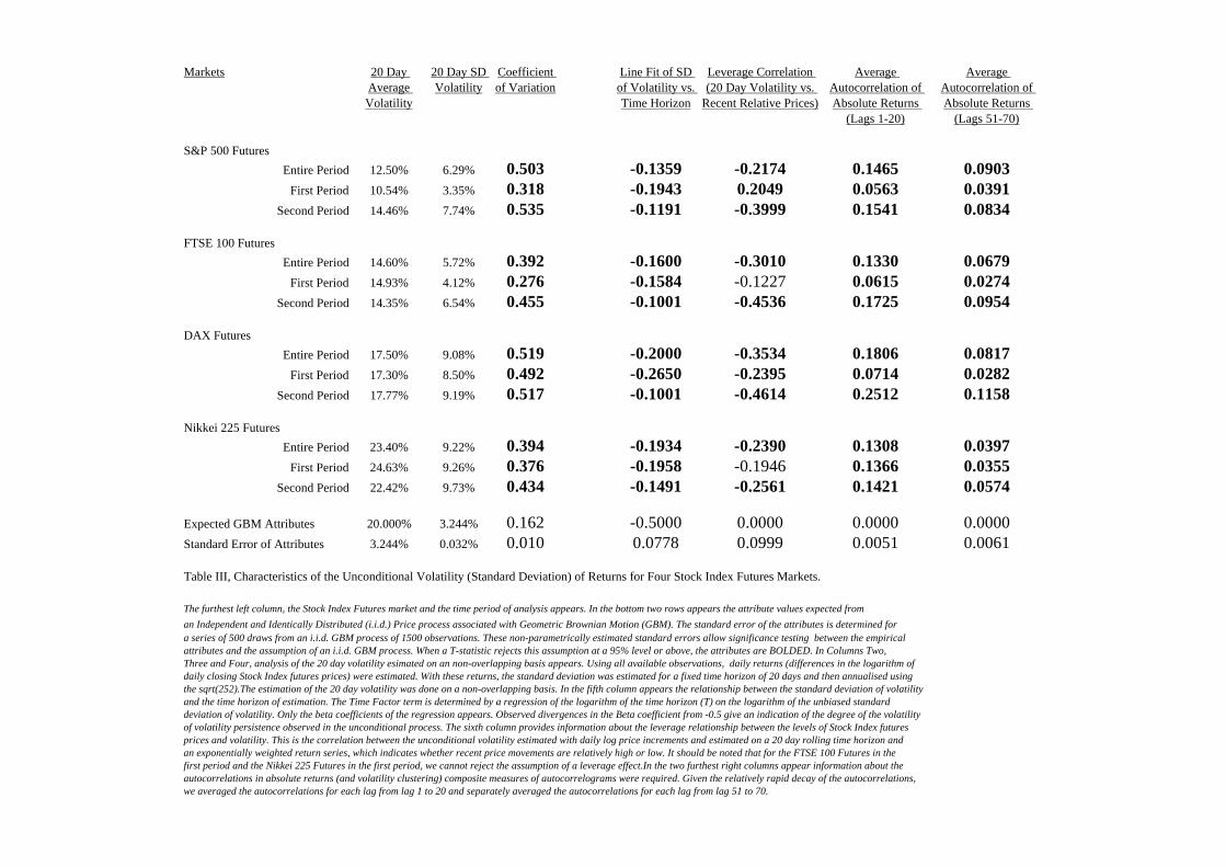
Markets 20 Day Average Volatility

20 Day SD Volatility

Coefficient of Variation

Line Fit of SD of Volatility vs. Time Horizon

Leverage Correlation (20 Day Volatility vs.

Recent Relative Prices)

Average Autocorrelation of Absolute Returns

(Lags 1-20)

Average Autocorrelation of Absolute Returns

(Lags 51-70)

S&P 500 FuturesEntire Period 12.50% 6.29% 0.503 -0.1359 -0.2174 0.1465 0.0903

First Period 10.54% 3.35% 0.318 -0.1943 0.2049 0.0563 0.0391Second Period 14.46% 7.74% 0.535 -0.1191 -0.3999 0.1541 0.0834

FTSE 100 FuturesEntire Period 14.60% 5.72% 0.392 -0.1600 -0.3010 0.1330 0.0679

First Period 14.93% 4.12% 0.276 -0.1584 -0.1227 0.0615 0.0274Second Period 14.35% 6.54% 0.455 -0.1001 -0.4536 0.1725 0.0954

DAX FuturesEntire Period 17.50% 9.08% 0.519 -0.2000 -0.3534 0.1806 0.0817

First Period 17.30% 8.50% 0.492 -0.2650 -0.2395 0.0714 0.0282Second Period 17.77% 9.19% 0.517 -0.1001 -0.4614 0.2512 0.1158

Nikkei 225 FuturesEntire Period 23.40% 9.22% 0.394 -0.1934 -0.2390 0.1308 0.0397

First Period 24.63% 9.26% 0.376 -0.1958 -0.1946 0.1366 0.0355Second Period 22.42% 9.73% 0.434 -0.1491 -0.2561 0.1421 0.0574

Expected GBM Attributes 20.000% 3.244% 0.162 -0.5000 0.0000 0.0000 0.0000Standard Error of Attributes 3.244% 0.032% 0.010 0.0778 0.0999 0.0051 0.0061

Table III, Characteristics of the Unconditional Volatility (Standard Deviation) of Returns for Four Stock Index Futures Markets.

The furthest left column, the Stock Index Futures market and the time period of analysis appears. In the bottom two rows appears the attribute values expected from an Independent and Identically Distributed (i.i.d.) Price process associated with Geometric Brownian Motion (GBM). The standard error of the attributes is determined fora series of 500 draws from an i.i.d. GBM process of 1500 observations. These non-parametrically estimated standard errors allow significance testing between the empiricalattributes and the assumption of an i.i.d. GBM process. When a T-statistic rejects this assumption at a 95% level or above, the attributes are BOLDED. In Columns Two, Three and Four, analysis of the 20 day volatility esimated on an non-overlapping basis appears. Using all available observations, daily returns (differences in the logarithm of daily closing Stock Index futures prices) were estimated. With these returns, the standard deviation was estimated for a fixed time horizon of 20 days and then annualised using the sqrt(252).The estimation of the 20 day volatility was done on a non-overlapping basis. In the fifth column appears the relationship between the standard deviation of volatility and the time horizon of estimation. The Time Factor term is determined by a regression of the logarithm of the time horizon (T) on the logarithm of the unbiased standard deviation of volatility. Only the beta coefficients of the regression appears. Observed divergences in the Beta coefficient from -0.5 give an indication of the degree of the volatility of volatility persistence observed in the unconditional process. The sixth column provides information about the leverage relationship between the levels of Stock Index futures prices and volatility. This is the correlation between the unconditional volatility estimated with daily log price increments and estimated on a 20 day rolling time horizon andan exponentially weighted return series, which indicates whether recent price movements are relatively high or low. It should be noted that for the FTSE 100 Futures in the first period and the Nikkei 225 Futures in the first period, we cannot reject the assumption of a leverage effect.In the two furthest right columns appear information about the autocorrelations in absolute returns (and volatility clustering) composite measures of autocorrelograms were required. Given the relatively rapid decay of the autocorrelations, we averaged the autocorrelations for each lag from lag 1 to 20 and separately averaged the autocorrelations for each lag from lag 51 to 70.

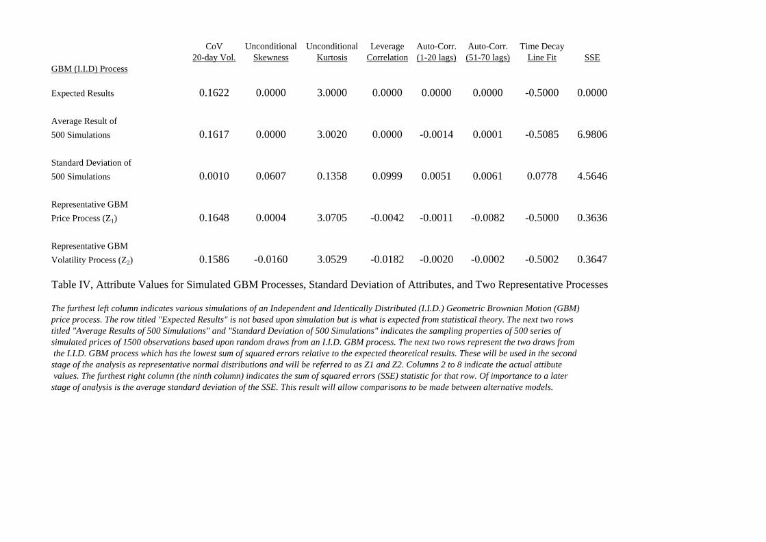
CoV Unconditional Unconditional Leverage Auto-Corr. Auto-Corr. Time Decay20-day Vol. Skewness Kurtosis Correlation (1-20 lags) (51-70 lags) Line Fit SSE

GBM (I.I.D) Process

Expected Results 0.1622 0.0000 3.0000 0.0000 0.0000 0.0000 -0.5000 0.0000

Average Result of500 Simulations 0.1617 0.0000 3.0020 0.0000 -0.0014 0.0001 -0.5085 6.9806

Standard Deviation of500 Simulations 0.0010 0.0607 0.1358 0.0999 0.0051 0.0061 0.0778 4.5646

Representative GBMPrice Process (Z1) 0.1648 0.0004 3.0705 -0.0042 -0.0011 -0.0082 -0.5000 0.3636

Representative GBMVolatility Process (Z2) 0.1586 -0.0160 3.0529 -0.0182 -0.0020 -0.0002 -0.5002 0.3647

Table IV, Attribute Values for Simulated GBM Processes, Standard Deviation of Attributes, and Two Representative Processes

The furthest left column indicates various simulations of an Independent and Identically Distributed (I.I.D.) Geometric Brownian Motion (GBM)price process. The row titled "Expected Results" is not based upon simulation but is what is expected from statistical theory. The next two rowstitled "Average Results of 500 Simulations" and "Standard Deviation of 500 Simulations" indicates the sampling properties of 500 series of simulated prices of 1500 observations based upon random draws from an I.I.D. GBM process. The next two rows represent the two draws from the I.I.D. GBM process which has the lowest sum of squared errors relative to the expected theoretical results. These will be used in the second stage of the analysis as representative normal distributions and will be referred to as Z1 and Z2. Columns 2 to 8 indicate the actual attibute values. The furthest right column (the ninth column) indicates the sum of squared errors (SSE) statistic for that row. Of importance to a later stage of analysis is the average standard deviation of the SSE. This result will allow comparisons to be made between alternative models.

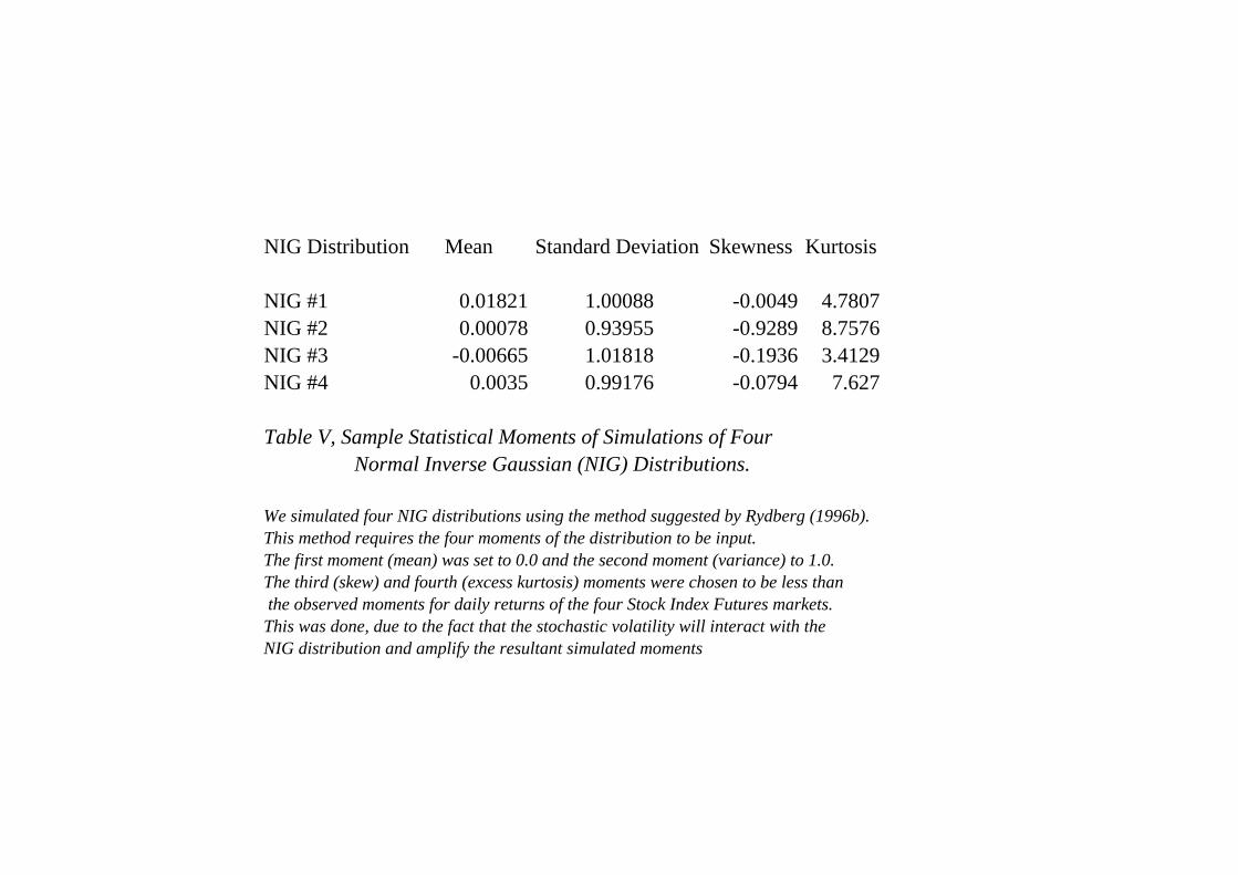
NIG Distribution Mean Standard Deviation Skewness Kurtosis

NIG #1 0.01821 1.00088 -0.0049 4.7807NIG #2 0.00078 0.93955 -0.9289 8.7576NIG #3 -0.00665 1.01818 -0.1936 3.4129NIG #4 0.0035 0.99176 -0.0794 7.627

Table V, Sample Statistical Moments of Simulations of FourNormal Inverse Gaussian (NIG) Distributions.

We simulated four NIG distributions using the method suggested by Rydberg (1996b). This method requires the four moments of the distribution to be input. The first moment (mean) was set to 0.0 and the second moment (variance) to 1.0. The third (skew) and fourth (excess kurtosis) moments were chosen to be less than the observed moments for daily returns of the four Stock Index Futures markets. This was done, due to the fact that the stochastic volatility will interact with the NIG distribution and amplify the resultant simulated moments

Models (Parameters) Empirical and Simulated Attributes

Empirical AttributesS&P 500 (Whole Period) CoV Skewness Kurtosis Leverage Corr(1-20) Corr(51-70) Line FitFutures 0.5033 -0.4397 11.4006 -0.2174 0.1465 0.0903 -0.1359

Distribution LTV K VoV Correl Simulated Attributes SSE T-StatisticModel 1 GBM 0.125 0.00 0.000 0 0.1648 0.0004 3.0705 -0.0042 -0.0011 -0.0082 -0.5000 255.781

Model 2 GBM 0.125 3.10 0.890 -0.25 0.4471 -0.4685 5.9502 -0.2742 0.1763 0.0765 -0.1086 6.571 54.651

Model 3 NIG-T1 0.125 1.80 0.380 -0.35 0.5239 -0.3702 9.6509 -0.2165 0.1597 0.0759 -0.1819 3.387 55.349

Empirical AttributesS&P 500 (First Period) CoV Skewness Kurtosis Leverage Corr(1-20) Corr(51-70) Line FitFutures 0.3180 0.2074 6.0778 0.2049 0.0563 0.0391 -0.1943

Distribution LTV K VoV Correl Simulated Attributes SSE T-StatisticModel 1 GBM 0.105 0.00 0.000 0 0.1648 0.0004 3.0705 -0.0042 -0.0011 -0.0082 -0.5000 123.538

Model 2 GBM 0.105 2.39 0.172 0.035 0.2928 0.0161 3.5894 0.1824 0.0852 0.0371 -0.1456 2.686 26.503

Model 3 NIG-T3 0.105 2.05 0.170 -0.09 0.2961 -0.1488 4.2690 0.1607 0.0701 0.0377 -0.1875 1.020 26.868

Empirical AttributesS&P 500 (Second Period) CoV Skewness Kurtosis Leverage Corr(1-20) Corr(51-70) Line FitFutures 0.5350 -0.6206 11.2081 -0.3999 0.1541 0.0834 -0.1191

Distribution LTV K VoV Correl Simulated Attributes SSE T-StatisticModel 1 GBM 0.145 0.00 0.000 0 0.1648 0.0004 3.0705 -0.0042 -0.0011 -0.0082 -0.5000 393.627

Model 2 GBM 0.145 4.00 0.700 -0.4 0.5072 -0.6220 6.5818 -0.3921 0.2139 0.0796 -0.1171 4.899 85.247

Model 3 NIG-T1 0.145 1.99 0.495 -0.61 0.5769 -0.5503 10.6853 -0.4214 0.1833 0.0872 -0.1568 2.885 85.689

Table VI a, Empirical Attributes of S&P 500 Futures and Attributes of Five Alternative ModelsThis table displays the empirical attributes (taken from Tables II and III) and the results of the models for the S&P 500 Futures. These results are split into the three periods of analysis. In each of these tables, the three time periods of analysis appear. On the left-hand side, the parameterisation of each of the three models appears. Only the parameter values and the NIG distribution that has the lowest SSE are presented. On the right-hand side, the simulated attributes of each model appear with the empirical attributes directly above for comparison's sake. In the column immediately to the right of this the sum of squared errors (SSE) for each model appears. The final column indicates a T-test statistic comparing models 2 and 3 to the GBM assumption. This is computed by taking the difference in the SSE for the models compared to the GBM case and dividing this by the simulated standard error of the SSE statistic found in Table IV.

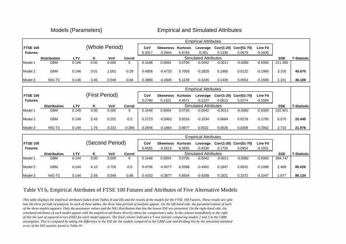
Models (Parameters) Empirical and Simulated Attributes

Empirical AttributesFTSE 100 (Whole Period) CoV Skewness Kurtosis Leverage Corr(1-20) Corr(51-70) Line FitFutures 0.3917 -0.0944 5.9793 -0.301 0.1330 0.0679 -0.1600

Distribution LTV K VoV Correl Simulated Attributes SSE T-StatisticModel 1 GBM 0.146 0.00 0.000 0 0.1648 0.0004 3.0705 -0.0042 -0.0011 -0.0082 -0.5000 211.355

Model 2 GBM 0.146 3.01 1.001 -0.29 0.4858 -0.4720 5.7005 -0.2829 0.1965 0.0122 -0.1969 3.100 45.670

Model 3 NIG-T3 0.148 3.45 0.549 -0.64 0.3869 -0.2845 5.1239 -0.3226 0.1439 0.0553 -0.1599 1.101 46.108

Empirical AttributesFTSE 100 (First Period) CoV Skewness Kurtosis Leverage Corr(1-20) Corr(51-70) Line FitFutures 0.2760 0.1322 4.4571 -0.1227 0.0615 0.0274 -0.1584

Distribution LTV K VoV Correl Simulated Attributes SSE T-StatisticModel 1 GBM 0.149 0.00 0.000 0 0.1648 0.0004 3.0705 -0.0042 -0.0011 -0.0082 -0.5000 102.921

Model 2 GBM 0.149 2.43 0.251 -0.2 0.2723 -0.0962 3.5016 -0.1034 0.0684 0.0278 -0.1795 0.570 22.445

Model 3 NIG-T3 0.149 1.76 0.223 -0.266 0.2646 -0.1864 3.9877 0.0522 0.0526 0.0308 -0.2062 2.710 21.976

Empirical AttributesFTSE 100 (Second Period) CoV Skewness Kurtosis Leverage Corr(1-20) Corr(51-70) Line FitFutures 0.4555 -0.2613 6.5835 -0.4536 0.1725 0.0954 -0.1001

Distribution LTV K VoV Correl Simulated Attributes SSE T-StatisticModel 1 GBM 0.144 0.00 0.000 0 0.1648 0.0004 3.0705 -0.0042 -0.0011 -0.0082 -0.5000 394.747

Model 2 GBM 0.144 4.10 0.750 -0.5 0.4706 -0.6577 6.5588 -0.4462 0.1847 0.0832 -0.1088 2.468 86.026

Model 3 NIG-T3 0.144 2.59 0.549 -0.86 0.4253 -0.3877 4.8504 -0.4268 0.1821 0.1072 -0.1047 1.977 86.134

Table VI b, Empirical Attributes of FTSE 100 Futures and Attributes of Five Alternative Models

This table displays the empirical attributes (taken from Tables II and III) and the results of the models for the FTSE 100 Futures. These results are split into the three periods of analysis. In each of these tables, the three time periods of analysis appear. On the left-hand side, the parameterisation of each of the three models appears. Only the parameter values and the NIG distribution that has the lowest SSE are presented. On the right-hand side, the simulated attributes of each model appear with the empirical attributes directly above for comparison's sake. In the column immediately to the right of this the sum of squared errors (SSE) for each model appears. The final column indicates a T-test statistic comparing models 2 and 3 to the GBM assumption. This is computed by taking the difference in the SSE for the models compared to the GBM case and dividing this by the simulated standard error of the SSE statistic found in Table IV.

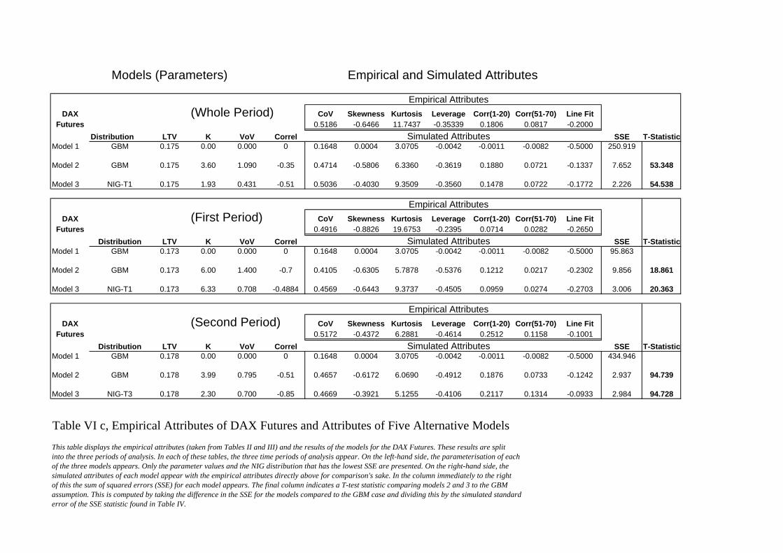
Models (Parameters) Empirical and Simulated Attributes

Empirical AttributesDAX (Whole Period) CoV Skewness Kurtosis Leverage Corr(1-20) Corr(51-70) Line Fit

Futures 0.5186 -0.6466 11.7437 -0.35339 0.1806 0.0817 -0.2000Distribution LTV K VoV Correl Simulated Attributes SSE T-Statistic

Model 1 GBM 0.175 0.00 0.000 0 0.1648 0.0004 3.0705 -0.0042 -0.0011 -0.0082 -0.5000 250.919

Model 2 GBM 0.175 3.60 1.090 -0.35 0.4714 -0.5806 6.3360 -0.3619 0.1880 0.0721 -0.1337 7.652 53.348

Model 3 NIG-T1 0.175 1.93 0.431 -0.51 0.5036 -0.4030 9.3509 -0.3560 0.1478 0.0722 -0.1772 2.226 54.538

Empirical AttributesDAX (First Period) CoV Skewness Kurtosis Leverage Corr(1-20) Corr(51-70) Line Fit

Futures 0.4916 -0.8826 19.6753 -0.2395 0.0714 0.0282 -0.2650Distribution LTV K VoV Correl Simulated Attributes SSE T-Statistic

Model 1 GBM 0.173 0.00 0.000 0 0.1648 0.0004 3.0705 -0.0042 -0.0011 -0.0082 -0.5000 95.863

Model 2 GBM 0.173 6.00 1.400 -0.7 0.4105 -0.6305 5.7878 -0.5376 0.1212 0.0217 -0.2302 9.856 18.861

Model 3 NIG-T1 0.173 6.33 0.708 -0.4884 0.4569 -0.6443 9.3737 -0.4505 0.0959 0.0274 -0.2703 3.006 20.363

Empirical AttributesDAX (Second Period) CoV Skewness Kurtosis Leverage Corr(1-20) Corr(51-70) Line Fit

Futures 0.5172 -0.4372 6.2881 -0.4614 0.2512 0.1158 -0.1001Distribution LTV K VoV Correl Simulated Attributes SSE T-Statistic

Model 1 GBM 0.178 0.00 0.000 0 0.1648 0.0004 3.0705 -0.0042 -0.0011 -0.0082 -0.5000 434.946

Model 2 GBM 0.178 3.99 0.795 -0.51 0.4657 -0.6172 6.0690 -0.4912 0.1876 0.0733 -0.1242 2.937 94.739

Model 3 NIG-T3 0.178 2.30 0.700 -0.85 0.4669 -0.3921 5.1255 -0.4106 0.2117 0.1314 -0.0933 2.984 94.728

Table VI c, Empirical Attributes of DAX Futures and Attributes of Five Alternative ModelsThis table displays the empirical attributes (taken from Tables II and III) and the results of the models for the DAX Futures. These results are split into the three periods of analysis. In each of these tables, the three time periods of analysis appear. On the left-hand side, the parameterisation of each of the three models appears. Only the parameter values and the NIG distribution that has the lowest SSE are presented. On the right-hand side, the simulated attributes of each model appear with the empirical attributes directly above for comparison's sake. In the column immediately to the right of this the sum of squared errors (SSE) for each model appears. The final column indicates a T-test statistic comparing models 2 and 3 to the GBM assumption. This is computed by taking the difference in the SSE for the models compared to the GBM case and dividing this by the simulated standard error of the SSE statistic found in Table IV.

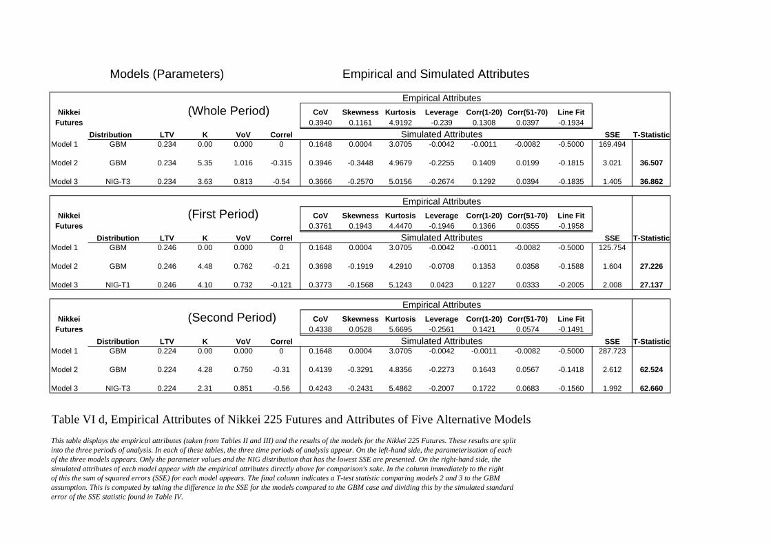
Models (Parameters) Empirical and Simulated Attributes

Empirical AttributesNikkei (Whole Period) CoV Skewness Kurtosis Leverage Corr(1-20) Corr(51-70) Line Fit

Futures 0.3940 0.1161 4.9192 -0.239 0.1308 0.0397 -0.1934Distribution LTV K VoV Correl Simulated Attributes SSE T-Statistic

Model 1 GBM 0.234 0.00 0.000 0 0.1648 0.0004 3.0705 -0.0042 -0.0011 -0.0082 -0.5000 169.494

Model 2 GBM 0.234 5.35 1.016 -0.315 0.3946 -0.3448 4.9679 -0.2255 0.1409 0.0199 -0.1815 3.021 36.507

Model 3 NIG-T3 0.234 3.63 0.813 -0.54 0.3666 -0.2570 5.0156 -0.2674 0.1292 0.0394 -0.1835 1.405 36.862

Empirical AttributesNikkei (First Period) CoV Skewness Kurtosis Leverage Corr(1-20) Corr(51-70) Line Fit

Futures 0.3761 0.1943 4.4470 -0.1946 0.1366 0.0355 -0.1958Distribution LTV K VoV Correl Simulated Attributes SSE T-Statistic

Model 1 GBM 0.246 0.00 0.000 0 0.1648 0.0004 3.0705 -0.0042 -0.0011 -0.0082 -0.5000 125.754

Model 2 GBM 0.246 4.48 0.762 -0.21 0.3698 -0.1919 4.2910 -0.0708 0.1353 0.0358 -0.1588 1.604 27.226

Model 3 NIG-T1 0.246 4.10 0.732 -0.121 0.3773 -0.1568 5.1243 0.0423 0.1227 0.0333 -0.2005 2.008 27.137

Empirical AttributesNikkei (Second Period) CoV Skewness Kurtosis Leverage Corr(1-20) Corr(51-70) Line Fit

Futures 0.4338 0.0528 5.6695 -0.2561 0.1421 0.0574 -0.1491Distribution LTV K VoV Correl Simulated Attributes SSE T-Statistic

Model 1 GBM 0.224 0.00 0.000 0 0.1648 0.0004 3.0705 -0.0042 -0.0011 -0.0082 -0.5000 287.723

Model 2 GBM 0.224 4.28 0.750 -0.31 0.4139 -0.3291 4.8356 -0.2273 0.1643 0.0567 -0.1418 2.612 62.524

Model 3 NIG-T3 0.224 2.31 0.851 -0.56 0.4243 -0.2431 5.4862 -0.2007 0.1722 0.0683 -0.1560 1.992 62.660

Table VI d, Empirical Attributes of Nikkei 225 Futures and Attributes of Five Alternative ModelsThis table displays the empirical attributes (taken from Tables II and III) and the results of the models for the Nikkei 225 Futures. These results are split into the three periods of analysis. In each of these tables, the three time periods of analysis appear. On the left-hand side, the parameterisation of each of the three models appears. Only the parameter values and the NIG distribution that has the lowest SSE are presented. On the right-hand side, the simulated attributes of each model appear with the empirical attributes directly above for comparison's sake. In the column immediately to the right of this the sum of squared errors (SSE) for each model appears. The final column indicates a T-test statistic comparing models 2 and 3 to the GBM assumption. This is computed by taking the difference in the SSE for the models compared to the GBM case and dividing this by the simulated standard error of the SSE statistic found in Table IV.

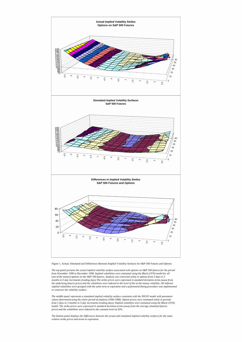
Figure 1, Actual, Simulated and Differences Between Implied Volatility Surfaces for S&P 500 Futures and Options

The top panel presents the actual implied volatility surface associated with options on S&P 500 futures for the period from November 1990 to December 1998. Implied volatilities were estimated using the Black (1976) model for all (out of the money) options on the S&P 500 futures. Analysis was restricted solely to options from 5 days to 3 months in 5-day increments (trading days) The strike prices were expressed in standard deviation terms (away from the underlying futures price) and the volatilities were indexed to the level of the at-the-money volatility. All indexed implied volatilities were grouped with the same term to expiration and a polynomial fitting procedure was implemented to construct the volatility surface.

The middle panel represents a simulated implied volatility surface consistent with the NIGSV model with parameter values determined using the entire period of analysis (1990-1998). Option prices were estimated solely to periods from 5 days to 3 months in 5-day increments (trading days). Implied volatilties were estimated using the Black (1976)model. The strike prices were expressed in standard deviation terms (away from the average simulated futuresprice) and the volatilities were indexed to the constant level of 20%.

The bottom panel displays the differences between the actual and simulated implied volatility surfaces for the same relative strike prices and terms to expiration.

-3.5 -3

-2.5 -2

-1.5 -1

-0.5 0

0.5 1

1.5 2

2.5 3

3.5

5

15

25

35455580

708090

100110120130140150160170180190

Simulated Implied Volatility SurfacesS&P 500 Futures

-3.5 -3

-2.5 -2

-1.5 -1

-0.5 0

0.5 1

1.5 2

2.5 3

3.5

5

15

25

35455580

0

20

40

60

80

Differences in Implied Volatility SmilesS&P 500 Futures and Options

-3.5 -3

-2.5 -2

-1.5 -1

-0.5 0

0.5 1

1.5 2

2.5 3

3.5

5

15

25

35455580

708090

100110120130140150160170180190

Actual Implied Volatility SmilesOptions on S&P 500 Futures