Objective Identification of Annular Hurricanes

Objective Identification of Annular Hurricanes

JOHN A. KNAFF

NOAA/NESDIS/Center for Satellite Applications and Research, Fort Collins, Colorado

THOMAS A. CRAM

Department of Atmospheric Science, Colorado State University, Fort Collins, Colorado

ANDREA B. SCHUMACHER

Cooperative Institute for Research in the Atmosphere, Colorado State University, Fort Collins, Colorado

JAMES P. KOSSIN

Cooperative Institute for Meteorological Satellite Studies, University of Wisconsin—Madison, Madison, Wisconsin

MARK DEMARIA

NOAA/NESDIS/Center for Satellite Applications and Research, Fort Collins, Colorado

(Manuscript received 26 March 2006, in final form 21 June 2007)

ABSTRACT

Annular hurricanes are a subset of intense tropical cyclones that have been shown in previous work to besignificantly stronger, to maintain their peak intensities longer, and to weaken more slowly than averagetropical cyclones. Because of these characteristics, they represent a significant forecasting challenge. Thispaper updates the list of annular hurricanes to encompass the years 1995–2006 in both the North Atlanticand eastern–central North Pacific tropical cyclone basins. Because annular hurricanes have a unique ap-pearance in infrared satellite imagery, and form in a specific set of environmental conditions, an objectivereal-time method of identifying these hurricanes is developed. However, since the occurrence of annularhurricanes is rare (�4% of all hurricanes), a special algorithm to detect annular hurricanes is developed thatemploys two steps to identify the candidates: 1) prescreening the data and 2) applying a linear discriminantanalysis. This algorithm is trained using a dependent dataset (1995–2003) that includes 11 annular hurri-canes. The resulting algorithm is then independently tested using datasets from the years 2004–06, whichcontained an additional three annular hurricanes. Results indicate that the algorithm is able to discriminateannular hurricanes from tropical cyclones with intensities greater than 84 kt (43.2 m s�1). The probabilityof detection or hit rate produced by this scheme is shown to be �96% with a false alarm rate of �6%, basedon 1363 six-hour time periods with a tropical cyclone with an intensity greater than 84 kt (1995–2006).

1. Introduction

A subset of tropical cyclones, referred to as annularhurricanes, were introduced and diagnosed in an obser-vational study (Knaff et al. 2003, hereafter K03). An

annular hurricane (AH), as observed in infrared (IR)imagery, has a larger-than-average size eye, symmetri-cally distributed cold brightness temperatures associ-ated with eyewall convection, and few or no rainbandfeatures. K03 used these features to subjectively iden-tify six AHs in the Atlantic and eastern–central NorthPacific tropical cyclone basins. Findings of K03 showthat AH formation was systematic, resulting from whatappeared to be asymmetric mixing of eye and eyewallcomponents of the storms that involved one or twopossible mesovortices—a contention supported by lim-ited aircraft reconnaissance data and satellite imagery.

Corresponding author address: John Knaff, NOAA/NESDIS/Office of Research and Applications, CIRA/Colorado State Uni-versity, Foothills Campus Delivery 1375, Fort Collins, CO 80523-1375.E-mail: [email protected]

FEBRUARY 2008 K N A F F E T A L . 17

DOI: 10.1175/2007WAF2007031.1

© 2008 American Meteorological Society

WAF2007031

The AHs were also shown to exist and develop in spe-cific environmental conditions that are characterized by1) relatively weak easterly or southeasterly verticalwind shear, 2) easterly winds and colder-than-averagetemperatures at 200 hPa, 3) a specific range (25.4°–28.5°C) of sea surface temperatures (SSTs) with smallvariations along the storm track, and 4) a lack of 200-hPa relative eddy flux convergence due to interactionswith the environmental flow. Weak easterly shear ishypothesized to promote the symmetric nature of AHsby canceling the effect of vertical wind shear induced bythe vortex interacting with gradients of planetary vor-ticity. With respect to maximum wind speed, AHs weresignificantly stronger, maintained their peak intensitieslonger, and weakened more slowly, than the averagetropical cyclone in these basins (see Fig. 3 in K03). Asa result, average official forecast intensity errors forthese types of tropical cyclones were 10%–30% largerthan the 5-yr (1995–99) mean official errors during thesame period with pronounced negative biases (e.g.,�17.1 kt for the 48-h forecast).

Since the formal documentation of AHs, also re-ferred to as “truck tire” or “doughnut” tropical cy-clones by some forecasters, there have been a few ide-alized numerical modeling studies that examine thecombined effect of environmental and beta-vortex-induced shear or “beta shear.” The beta shear resultsfrom the differential advection of planetary vorticitywithin the tropical cyclone with height and weakeningof the beta gyres (Chan and Williams 1987; Fiorino andElsberry 1989) as a result of the cyclone’s warm corestructure (Wang and Holland 1996a,b,c; Bender 1997;Peng et al. 1999; Wu and Braun 2004; Ritchie and Frank2007). The majority of previous idealized numericalstudies of tropical cyclones were conducted on an fplane, primarily to keep the influence of planetary vor-ticity and its influences on motion and vertical windshear separate from other processes of interest. In gen-eral, f-plane simulations result in quite symmetric simu-lated tropical cyclones in the absence of vertical windshear, but the occurrence or development of AH-typestructures (i.e., symmetric with a large, temporally in-variant radius of maximum winds) to our knowledgehas not been explicitly reported or examined. However,it has been established that rather small magnitudes(��3 m s�1) of vertical wind shear lead to convectiveasymmetries and corresponding weakening of the vor-tex in such simulations (e.g., Ritchie and Frank 2007).

Recently, there has been renewed interest in the ef-fect of the advection of planetary vorticity on the evo-lution of tropical cyclone structure. The inclusion ofthese effects, in an environment at rest, has also pro-duced a more asymmetric and slightly larger tropical

cyclone that intensifies slightly slower than its f-planecounterpart in terms of minimum sea level pressure(MSLP) (Ritchie and Frank 2007). Wu and Braun(2004) produced similar results in tropical cyclonesimulations where the inclusion of beta shear results inmore asymmetries and a weaker tropical cyclone. Inanother study, Kwok and Chan (2005) found that uni-form westerly steering flow in variable-f simulationspartially cancels the beta shear, while easterly uniformsteering flow enhances it—findings that confirm earlierresults presented in Peng et al. (1999). The greaterasymmetry in tropical cyclone (TC) structure in theseTC simulations is in a large part due to the vertical windshear variations that result from the inclusion of theplanetary vorticity advection. Simulations of tropicalcyclones using environmental conditions similar tothose documented in K03 have also been shown to re-sult in a more axisymmetric tropical cyclone (Ritchie2004). One can interpret these results as implying thatbeta shear in these simulations produces greater TCasymmetries, and if the environmental wind shear op-poses the beta shear, these asymmetries are reduced.Furthermore, if the environmental conditions nearlycancel the beta shear, the TC can be axisymmetric,which supports the suggestions made in K03 that annu-lar hurricanes form in environments where the environ-mental vertical wind shear nearly cancels the beta shearand further intensification is limited by less than idealthermodynamic conditions (i.e., atypically low SSTsconditions).

AHs are intense tropical cyclones with average in-tensities greater than 100 kt (or 51 m s�1)—major hur-ricanes, and, despite their less-than-optimal thermody-namic conditions (i.e., SSTs � �28.5°C), they maintainintensities close to their maximum potential intensitywith respect to SST (e.g., DeMaria and Kaplan 1994b).Because of this intensity change behavior, intensities ofpast AHs have been consistently underforecast. Themean intensity of AHs makes them potentially high-impact events when they affect coastal areas. Objectiveidentification of AHs in an operational setting couldhelp forecasters better predict future intensity changesfor these tropical cyclones, and likely reduce the overallintensity forecast errors. This could be accomplished bysubjectively forecasting slower weakening or no weak-ening while AH conditions exist. K03 recognized theneed for better identification of AHs and suggestedmethods that used environmental conditions and IRimagery separately to identify, in a dependent manner,the six AHs that occurred in the Atlantic and eastern–central North Pacific during 1995–99. This paper ex-pands on those ideas and the results of recent modelingstudies to create a method to objectively identify AHs.

18 W E A T H E R A N D F O R E C A S T I N G VOLUME 23

This objective method, which uses information aboutthe storm’s environmental conditions, intensity, and ap-pearance in IR satellite imagery, is described in thefollowing sections.

2. Data and approach

In K03 the developmental data for the StatisticalHurricane Intensity Prediction Scheme (SHIPS; De-Maria and Kaplan 1994a, 1999; DeMaria et al. 2005)were used to determine the environmental conditionsassociated with AHs. Following the logic of K03, theSHIPS developmental data (SDD) are used in a similarway in this study, but the calculations used to create theSDD have continued to evolve. The largest changes tothe SDD involve how vertical wind shear was calcu-lated. The vertical shear calculation used in K03 wasaveraged in a circular area within a radius of 600 kmfollowing a Laplacian filtering procedure that was usedto remove the effects of the TC vortex as described inDeMaria and Kaplan (1999). In the current version ofSDD, no attempt is made to remove the storm vortexand an annular average (200–800 km) is used to esti-mate the environmental vertical wind shear. The cur-rent SDD also uses the National Centers for Environ-mental Prediction–National Center for AtmosphericResearch (NCEP–NCAR) reanalyses (Kalnay et al.1996) prior to 2001 and the NCEP Global Forecast Sys-tem (GFS; Lord 1993) analyses thereafter. SST esti-mates are still estimated from Reynolds’s (1988) weeklySST fields. The position of the tropical cyclone and itsintensity come from the National Hurricane Center(NHC) best track (Jarvinen et al. 1984). Note that be-cause tropical cyclone intensity is reported and ar-chived in units of knots (kt; 1 kt � 0.51 m s�1), this unitwill be used for intensity throughout this manuscript.Because of these changes, the latest version of the SDD(see DeMaria et al. 2005) at 6-h intervals for 1995–2006is used for this study, where the period 1995–2003 isused as a dependent dataset and 2004–06 are retainedfor independent testing.

In addition to the SDD, Geostationary OperationalEnvironmental Satellite (GOES) IR imagery withwavelengths centered near 10.7 �m is used in the formof 4-km Mercator projections during the period 1995–2006. The GOES IR imagery is taken from the Coop-erative Institute for Research in the Atmosphere(CIRA) Tropical Cyclone IR Archive (Mueller et al.2006; Kossin et al. 2007). Individual images wererenavigated to storm-centric coordinates using cubic-spline interpolated best-track positions (Kossin 2002).The time interval between images is generally 30 min,with the exception of the satellite “eclipse” periods oc-

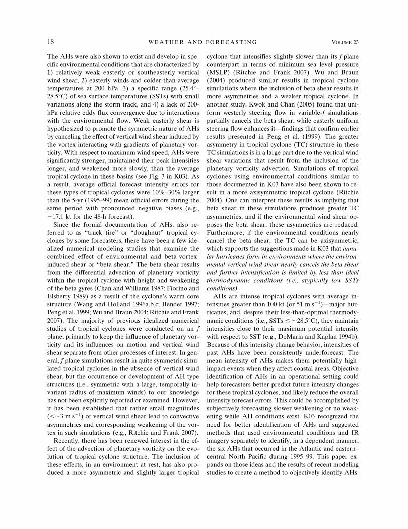
curring within approximately a month of the autumnalequinox and the last 1–3 h. In this study IR brightnesstemperature (TB) is azimuthally averaged about thestorm center and time averaged over a 6-h time period,corresponding to the 6 h prior to the analysis time. Thistime interval corresponds to the times in the NHC besttrack and the times in SDD. Figure 1 shows an IRimage of eastern North Pacific Hurricane Daniel on 27July 2001 at 2200 UTC, and the corresponding radialprofiles azimuthal mean and standard deviation of TB.Some of the characteristics of annular hurricanes can bequantified directly from these data (e.g., the existenceof large warm eye features or the relative lack of rain-band activity).

Changes in how environmental conditions have beenderived in the updated SDD require that the statisticsof the environmental conditions associated with theoriginal six AHs be recalculated. Using the most recentSDD and the IR image archive, statistics of key envi-ronmental conditions and IR imagery characteristics as-sociated with the six AHs described in K03 are shownin Table 1. Thirty-six 6-h time periods make up eachaverage. The average quantities calculated from the IRimagery and shown in Table 1 include the radius ofcoldest azimuthally averaged TB (Rc) as illustrated inFig. 1, the azimuthal standard deviation at Rc (�c) alsoshown in Fig. 1, the variance of the azimuthally aver-aged temperatures from the TC center to 600 km(VAR), and the maximum difference between TB atRc and any azimuthally averaged TB at smaller radii(�Teye). Table 1 also includes the statistics associatedwith the SSTs interpolated to the TC center (SST), themagnitude of the 200–850-hPa wind shear vector(SHRD), the magnitude of the 500–850-hPa wind shear(SHRS) vector, the zonal wind component at 200 hPa(U200), the temperature at 200 hPa (T200), the relativeeddy flux convergence (REFC; see K03), and the best-track value of maximum wind speed (Vmax). TheSHRD, SHRS, U200, and T200 parameters were calcu-lated in a 200–800-km annulus centered on the TC andthe REFC was calculated within 600 km of the TC cen-ter as described in DeMaria et al. (2005). These statis-tics are consistent with the environmental and visualcharacteristics of annular hurricanes (i.e., K03, theirTable 3 and Fig. 7). Small differences do occur due tothe differences in how the SDD parameters are calcu-lated, and the use of 6-h versus the 12-h time-averagingperiods used in K03. These new statistics are used as astarting point to develop an objective identificationtechnique discussed in the next section.

Since the publication of K03, a few more annularcases have occurred in the Atlantic and eastern NorthPacific. There has also been an opportunity to examine


some IR imagery prior to 1997 in the eastern Pacific.The expanded list of subjectively identified AHs for theperiod 1995–2006 is shown in Table 2. Eight cases, sev-eral short lived (i.e., Erin in 2001, Kate in 2003, andFrances in 2004 in the Atlantic, and Daniel in 2000 andBud in 2006 in the eastern Pacific) were added to thelist. However, since 2000, there have been a couple ofexceptional AH cases. Hurricanes Isabel (2003) andDaniel (2006) were both spectacular examples of AHs.Hurricane Isabel had four distinct periods with AHcharacteristics, each following a rearrangement of theeye, and Hurricane Daniel (2006) exhibited classic AHformation with eye-to-eyewall mixing, indicated by oneor more mesovortices seen in the IR imagery, followedby the formation of a large warm eye and diminishedrainband activity that lasted over 30 h.

The GOES IR satellite imagery associated with these14 subjectively identified AH cases for 1995–2006 (Fig.2) shows a large variety of sizes. The Atlantic AHs(yellow text), in general, appear larger than the east-ern–central North Pacific AHs (cyan text). In fact, the

average 34-kt wind radius is 109 n mi (202 km) and 135n mi (250 km) for the eastern–central North Pacific andAtlantic cases, respectively. These results are consistentwith the tropical cyclone size climatology of these ba-sins (Knaff et al. 2007) and cyclone sizes reported inKnaff and Zehr (2007), where 25 n mi (46 km) separatethe average 34-kt wind radius between the East Pacificand Atlantic basins. One could speculate that environ-mental conditions in the eastern–central North Pacificare less conducive for TC growth because upper-leveltrough interaction, and extratropical transition, both re-lated to TC growth (Maclay 2006; Maclay et al. 2007,manuscript submitted to Mon. Wea. Rev.), occur lessfrequently in that basin. The average AH intensity is110 kt (56.6 m s�1) and ranged from a low of 90 kt (46m s�1) to a high of 140 kt (72 m s�1). From the subjec-tively determined time periods in Table 2, the averageduration of an AH is approximately 18 h with a maxi-mum of 57 h associated with Hurricane Howard in1999. There also appears to be a preferred climatologi-cal time for formation. Eastern–central North Pacific

FIG. 1. (left) Storm-centered IR image of east Pacific Hurricane Daniel at 2200 UTC 27 Jul 2000 and (top right) the correspondingradial profiles of azimuthally averaged brightness temperatures with an arrow pointing to the radius of coldest average brightnesstemperature indicated as Rc and (bottom right) the azimuthal std devs with an arrow pointing to the value of the std dev at Rc andidentified as �c. The yellow circle centered within the image has a radius of 300 km for reference.


Fig 1 live 4/C

AHs tend to form from mid-July to late Augustwhereas Atlantic AH occurrence seems to be from mid-August to mid-October. Figure 3 shows the tracks as-sociated with the 14 AHs listed in Table 2. Thesestorms are not typically a threat to the U.S. mainland,but rather may be more of a concern for the Windward,Leeward, and Hawaiian Islands. There appears to be a

preferred location near 15°N and 125°W in the easternNorth Pacific while Atlantic AHs show greater variabil-ity in their locations. It is also important to note that theinclusion of the new cases does not change the findingsof K03 related to AH intensity behavior. The AHs werestill found to be significantly stronger, maintained theirpeak intensities longer, and weakened more slowlythan the average of all hurricanes.

3. Algorithm development

As described in K03, AHs occur in specific environ-mental conditions, characterized by a combination ofweak easterly or southeasterly vertical wind shear indeep-layer mean easterlies and relatively cold tempera-tures at 200 hPa, moderate SST, and relatively small200-hPa relative eddy flux convergence (REFC) due toenvironmental interactions. The AHs also appear dis-tinctly more axisymmetric in IR satellite imagery withlarge circular eyes surrounded by a nearly uniform ringof convection and a relative lack of deep convectivefeatures, including rainbands outside that ring. Fromresults presented in K03, it also appears that the envi-ronmental conditions can be combined with the IR sat-ellite imagery–derived characteristics of AHs to sepa-rate the population of annular hurricanes from thelarger population of nonannular hurricanes. At firstglance, this process would seem straightforward, butAHs are also rare events that occur in less than 4% ofall hurricane cases, which makes many standard statis-tical identification algorithms impractical.

TABLE 2. List of the 14 AH cases identified in the Atlantic and east Pacific Hurricane basins (1995–2006). Listed are the storm, basin,the times associated with the AH phase, the number of hours that each AH phase lasted, and the intensity range associated with thestorm.

Storm Basin Annular period Duration (h) Intensity range (kt)

Luis 1995 Atlantic 1800 UTC 3 Sep–0400 UTC 4 Sep 10 120–125Edouard 1996 Atlantic 0000 UTC 25 Aug–0000 UTC 26 Aug 24 120–125Erin 2001 Atlantic 0400 UTC 10 Sep–0900 UTC 10 Sep 6 100–105Isabel 2003 Atlantic 0700 UTC 11 Sep–2100 UTC 11 Sep 14 135–145

1000 UTC 12 Sep–2200 UTC 12 Sep 12 1401400 UTC 13 Sep–0200 UTC 14 Sep 12 135–1400700 UTC 14 Sep–2000 UTC 14 Sep 14 135–140

Kate 2003 Atlantic 1700 UTC 03 Oct–0000 UTC 4 Oct 5 1000400 UTC 04 Oct–1300 UTC 4 Oct 10 100–105

Frances 2004 Atlantic 2100 UTC 28 Aug–0200 UTC 29 Aug 6 115Barbara 1995 East Pacific 0500 UTC 14 Jul–1400 UTC 14 Jul 10 115–120Darby 1998 East Pacific 1200 UTC 26 Jul–1800 UTC 27 Jul 30 90–100Howard 1998 East Pacific 1800 UTC 24 Aug–0300 UTC 27 Aug 57 115–85Beatriz 1999 East Pacific 1800 UTC 12 Jul–1800 UTC 13 July 24 100–105Dora 1999 East Pacific 1800 UTC 10 Aug–0300 UTC 12 Aug 33 115–120

0300 UTC 15 Aug–0300 UTC 16 Aug 24 90–95Daniel 2000 East Pacific 2000 UTC 27 Jul–0400 UTC 28 Jul 9 95Bud 2006 East Pacific 0700 UTC 13 Jul–1300 UTC 13 Jul 6 100Daniel 2006 East Pacific 1400 UTC 21 Jul–2200 UTC 22 Jul 33 120–130

TABLE 1. Statistics of the important environmental conditionsand IR imagery–derived characteristics related to AHs. Statisticsare shown for the radius of coldest azimuthally averaged TB (Rc),the azimuthal standard deviation at Rc (�c), the variance of theazimuthally averaged temperatures from the TC center to 600 km(VAR), the maximum difference between Rc and any azimuthallyaveraged TB at smaller radii (�Teye), the SSTs interpolated tothe TC center (SST), the magnitude of the 200–850-hPa windshear vector (SHRD), the magnitude of the 500–850-hPa windshear (SHRS) vector, the zonal wind component at 200 hPa(U200), the temperature at 200 hPa (T200), the relative eddy fluxconvergence (REFC), and the best-track value of maximum windspeed (Vmax).

Quantity (units) Mean Std dev Min Max

Rc (km) 80.9 19.7 62.0 128.0�c (°C) 3.0 1.1 1.5 5.8VAR (°C2) 712.1 141.3 391.2 978.6�Teye (°C) 69.3 13.5 19.6 79.9SST (°C) 26.7 0.7 25.4 28.4SHRD (m s�1) 4.0 1.5 1.2 8.1SHRS (m s�1) 3.2 1.2 0.7 6.0U200 (m s�1) �4.8 2.3 �7.2 0T200 (°C) �52.2 0.9 �53.4 �50.1REFC (m s�1 day�1) 0.2 1.2 �4.0 4.0Vmax (kt) 107.2 12.8 85.0 125.0


To find the relatively rare occurrences of AHs in thecombined Atlantic and eastern–central North PacificTC sample, a two-step algorithm is developed. The firststep is to prescreen the SDD and IR satellite data forcases when the environmental conditions and IR satel-lite TB distribution are unfavorable for AHs. The sec-ond step is to apply a statistical technique called linear

discriminant analysis (LDA; see Wilks 2006) to theSSD and IR satellite dataset that remains after thescreening step. LDA is a formal technique that dis-criminates between two or more populations using lin-ear combinations of a set of discriminators. To test theability of this two-step algorithm to discriminate eventsfrom nonevents, we use the hit rate and the false alarm

FIG. 2. Color-enhanced GOES IR satellite imagery of the 14 annular hurricane cases at or near peak visual annular characteristics.Storm names, dates, and times are given at the bottom of each individual image panel. In addition, storm names and years are listedin the upper left of each image panel with North Atlantic and eastern–central North Pacific storm names indicated by yellow and cyantext, respectively.

FIG. 3. Map of the tracks of the 14 annular hurricane cases used in this study. The time periods when thesehurricanes were subjectively identified to be annular hurricanes are indicated by the thick black portion of thetrack.


Fig 2 live 4/C

rate (Mason and Graham 1999). The hit rate is thenumber of correctly identified AH cases divided by thenumber of AHs observed and the false alarm rate isthe number of incorrectly identified AH cases dividedby the total number of nonannular hurricane (NAH)cases observed, which for this study includes allstorms that passed the screening and were not AHs.One caveat to this study is that the subjectively identi-fied AH cases are used to develop and then indepen-dently test this objective technique, which is far fromideal and will likely degrade the final algorithm (sec-tion 4).

For the screening step, a set of “selection” rules aredetermined to eliminate cases where AHs are very un-likely to occur given the environmental conditions andIR characteristics. These criteria are listed in Table 3.To be as inclusive as possible, the environmental dis-criminators were set to values that capture the 54 six-hour time periods associated with the 11 AHs that oc-curred during 1995–2003. The thresholds for storm in-tensity, �Teye and Rc, which are far from normallydistributed, are set to values slightly less than theminima of the AH sample. The SST is used as anothercriterion to eliminate NAH cases since AHs are ob-served to occur in a distinct range of SST values. TheSST thresholds are based on the mean �3 standarddeviations of the annular group sample. The selectionrules were applied to the original data sample (1995–2003) that contained 976 six-hour tropical cyclone caseswith intensities greater than 84 kt. After the selectionrules were applied, there were 241 remaining 6-h cases,of which 53 were objectively identified and subjectivelyconfirmed as being AHs (1 case was missing quality IRsatellite imagery). Thus, the prescreening of the depen-dent dataset had a 100% hit rate, but a false alarm rateof 19%, given the 972 cases that passed the screening.Using LDA, we hope to improve the false alarm rate.

LDA is then used to take advantage of differencesbetween the AH and NAH samples. From the 1995–2003 cases, the environmental factors that had signifi-cant annular versus nonannular differences were used

as discriminators in the LDA. Results show that anenvironment characterized by lower SSTs and easterlyzonal 200-hPa winds and IR imagery depicting warmeyes, a radius of the coldest pixel (i.e., inner-core con-vection) with little azimuthal variability, and a less vari-able radial profile of brightness temperatures (i.e.,fewer rainbands) form the basis for discriminating AHsfrom NAHs in the screened sample. The environmentaldiscriminators therefore are 1) SST and 2) U200. Simi-larly, the IR-based discriminators used are 1) �c, 2)VAR, and 3) �Teye. All of the above discriminatorswere chosen based on their statistical significance (i.e.,exceeding the 95% significance level using a two-tailedStudent’s t test) between the sample data means of theAH and NAH cases that passed the prescreening pro-cess. The storm cases chosen to belong to the group ofAHs in the LDA development are the 11 cases with 53six-hour periods subjectively determined to be AHslisted in Table 1 for the period 1995–2003.

The prescreened data have been normalized prior tocarrying out the LDA by subtracting the sample meanand then dividing by the sample standard deviation foreach discriminator. Standardizing the input data allowsone to estimate the relative importance of each param-eter in the LDA. LDA then provides the normalizedweights for the linear combination of the input vari-ables that best differentiates between AH and NAHcases. Table 4 shows the normalized discriminantweights produced by the LDA. Also shown in Table 4are the means and standard deviations associated withthe parameter calculated from the 241 prescreenedcases, which are used for parameter normalization.When the discriminant vector is applied, positive valuesare indicative of AHs. Noting that the prescreening re-quires a large eye and a low vertical shear environment,Table 4 indicates that the largest contribution to thediscrimination comes from the factors associated withSST, and VAR (i.e., variance of the radial profile ofazimuthal mean brightness temperatures), which is ameasure of significant rainband activity.

TABLE 3. Summary of selection rules used to prescreen the in-put data and remove cases when an AH event is unlikely. Vari-ables as in Table 1.

Parameter Source Prescreening criterion

Rc IR satellite imagery �50 km�Teye IR satellite imagery �15°CSHRD NCEP–NCAR analysis 11.3 m s�1

U200 NCEP–NCAR analysis ��11.8 or 1.5 m s�1

REFC NCEP–NCAR analysis ��9 or 11 m s�1 day�1

SST Reynolds SST �24.3 or 29.1°CIntensity NHC best track �85 kt

TABLE 4. Normalized coefficients of the AH discriminant vec-tor based upon the 1995–2002 AH cases. Variables as in Table 1.Note the discriminant divider is a unitless number that causes thediscriminant function values to be centered about a zero value.

Discriminator Mean Std devNormalizedcoefficient

�c 4.21 2.56 �0.40VAR 552.73 215.10 0.79�Teye 59.67 20.99 0.50U200 �3.72 2.88 �0.11SST 27.58 1.08 �0.61Discriminant divider 0.53


The linear combination of the normalized discrimi-nant weights and the standardized input variables forboth AH and NAH cases are then calculated to deter-mine the value of the discriminant function at eachanalysis time. Although the LDA is designed to pro-duce a yes–no answer, the range of values of the dis-criminant function performed on the dependent datasample allows us to assign a normalized annular hurri-cane index value to each case. The relative magnitudeof the discriminant value is an indicator of how “annu-lar” a particular case is.

The results from the linear discriminant function,however, are not perfect and misidentified 56 of 188NAH cases as being annular and 7 of the 53 AH casesas being NAH. Using the dependent sample and com-bining the two steps (i.e., prescreening and LDA)shows that the algorithm identified 46 of the 53 six-hourperiods when AH existed and had a hit rate of 87%,while only falsely identifying 56 cases as AH out of 923eighty-four-kt or greater 6-h NAH cases resulting in afalse alarm rate of �6%. The seven false negatives oc-curred with 1) short-lived annular hurricanes (Luis in1995, Erin in 2001, and Kate in 2003), which accountedfor four cases, and 2) cases associated the first 6-h pe-riod in the annular phase. These false negative caseshad an average discriminant value of 0.39 and only onecase (Beatriz) had a value greater than 1.25, which wasdue to the rapid evolution of Beatriz and the time av-eraging applied to the IR TB data. Most of the falsepositives were associated with AHs but at times before

or after their subjectively determined annular phase(s).The average of the discriminant value for these 56 caseswas �0.76. Other false positives that were never AHsinclude the east Pacific Hurricanes Felicia (1997),Guillermo (1997), Georgette (1998), Adolf (2001), Her-nan (2002), and Jimena (2003) with two, one, three,one, two, and two 6-hourly time periods misidentified,respectively. Similarly Atlantic Hurricanes Georges(1998), Alberto (2000), Isidore (2000), and Fabian(2003) had two, one, one, and one 6-h time periods thatwere misidentified, respectively. Figure 4 shows the cu-mulative probability diagrams for the AH and NAHcases as a function of the discriminant value, whichshows the LDA properly discriminating the majority ofthe cases with a larger probability of false identificationthan of false alarm rate. For the final algorithm (section4), it will be desirable to maximize the hit rate whileminimizing the false alarms through scaling of the dis-criminant function values using information in such dia-grams.

It is interesting to examine what the LDA is actuallydiscriminating. To briefly show what the LDA algo-rithm determines as an AH case versus a NAH case,four time periods of Hurricane Isabel with varying de-grees of AH characteristics are examined. Figure 5shows IR imagery of Hurricane Isabel and correspond-ing discriminant value at 0345 UTC 11 September, 1145UTC 12 September, 0345 UTC 14 September, and 1145UTC 18 September. The 0345 UTC time is the lastimage used for the annular index estimation at 0600

FIG. 4. The cumulative probability distributions associated with the dependent data (1995–2003) as a function of binned discriminant function values created by the LDA. The dashedline is for the NAH cases and the solid line is for the AH cases.


UTC due to satellite eclipse times.1 Notice that as Isa-bel changes from an asymmetric hurricane on 11 Sep-tember to an AH on 12 September, the discriminantvalue goes from negative to positive. On 14 September

at 0345 UTC, following a separate annular period on 13September through early on 14 September (not shown),the storm displays a distinct banding structure in theenhanced temperatures that wraps around the storm,instead of a more continuous ring of nearly constanttemperatures, and thus is a NAH. The image on 18September shows an example of an extreme NAH case.For these four images the environment is also varying,which also contributes to the estimate of the discrimi-

1 Note that some recently launched operational geostationarysatellites (i.e., GOES-13, Meteosat-8, and Meteosat-9) operatethrough the eclipse periods.

FIG. 5. Examples of GOES IR satellite imagery from Hurricane Isabel (2003) and corresponding discriminantfunction values (dv) shown in the upper center of each panel. Results are based upon dependent data and negativevalues of dv discriminate AH cases. Imagery times are (top left) 0345 UTC 11 Sep, (top right) 1145 UTC 12 Sep,(bottom left) 0345 UTC 14 Sep, and (bottom right) 1145 UTC 18 Sep, and are also shown at the bottom of eachpanel.


Fig 5 live 4/C

nant value. The 200-hPa zonal winds were �6.7, �3.0,0.7, and �1.5 m s�1 and the SSTs were 28.4, 28.2, 28.4,and 27.5°C, in these images, respectively. During theperiod between 11 and 18 September, the algorithmproperly (improperly) identified 8 (8) of the AH peri-ods and 12 (0) of the NAH periods as Isabel wentthrough four separate 12–14-h subjectively identifiedAH periods.

In summary, an algorithm to detect AHs is createdusing a two-step process. The first step is to prescreenthe data using known environmental and storm-scalefactors that are indicative of AHs. This step reduces thesample from 976 hurricane 6-h cases that have intensi-ties greater than or equal to 85 kt to 241 cases thatcould be AHs. The second step is to create an LDAalgorithm to identify AHs using the period 1995–2003,incorporating those remaining 241 six-hour cases. Theoutput of the LDA, the discriminator function, is anobjective measure of whether a storm is or is not an AHand how “annular” a particular case is. This two-stepalgorithm is illustrated schematically in Fig. 6 and isapplied to independent data and tested in the next sec-tion.

4. Independent testing and final algorithm

The algorithm discussed in the previous section istested using independent datasets collected during2004–06. This involves applying the LDA coefficientsshown in Table 4 to the SDD and IR satellite imageryresults during those seasons, to objectively identify theAH periods shown in Table 2. During the years 2004–06 there were 2424 total 6-h cases of which 387 hadintensities greater than 84 kt and 82 passed the pre-screening process. Of these remaining 82 cases, 21 caseswere objectively identified as AHs and 61 cases wereidentified as NAHs. Of the objectively identified AHcases, seven were associated with times listed in Table2. Of the subjectively identified times 7 out 7 wereproperly identified, leaving 14 false positive cases. Ofthe 14 false positive 6-h cases, only 3 were associatedwith Hurricane Jova of 2005, which never became anAH. The result of the 3-yr independent test is that thetwo-step objective AH identification scheme identified100% of the AH cases with a false alarm rate of �4%,noting that there were 380 NAHs.

The results of the independent and dependent testingof the two-step objective AH identification schemeshow that AHs can be identified objectively and in areal-time manner. With a goal of creating a real-timeAH identification index, the next step is to use theentire dataset to estimate a final set of LDA coeffi-cients. There were 1363 six-hour cases that had inten-sities greater than 84 kt, and screening produced 323cases for the LDA. Table 5 shows the normalized pa-rameter weights determined by the LDA, and themeans and standard deviations of the 323 screenedcases in the 12-yr sample (1995–2006). ComparingTables 4 and 5, the addition of the 2004–06 cases haschanged the weights in such a way that all of the vari-ables except VAR have a larger influence on the dis-criminant function.

To more easily interpret the discriminant function,the discriminant values for annular hurricanes are

FIG. 6. Schematic of the two-step procedure used to objectivelyidentify AHs.

TABLE 5. Normalized coefficients of the AH discriminant vec-tor based upon the 1995–2006 AH cases. Variables as in Table 1.Note the discriminant divider is a unitless number that causes thediscriminant function values to be centered about a zero value.

Discriminator Mean Std devNormalizedcoefficient

�c 4.23 2.45 �0.44VAR 558.21 218.52 0.61�Teye 56.73 21.61 0.81U200 �4.55 2.89 �0.15SST 27.68 1.04 �0.80Discriminant divider 0.76


scaled from 0 to 100 so that a value of 0 indicates theanswer “not an AH,” a value of 1 indicates the possi-bility of a AH with the least likelihood, and a value of100 indicates an AH with the greatest likelihood. Dis-criminant values of �0.3 and 2.3 correspond to scaledindex values of 1 and 100, respectively, and scaled indexvalues are also set to 0 and to 100 for discriminantfunction values less than (greater than) than �0.3 and2.3, respectively. These values represent an objectivedegree of AH characteristics that are satisfied andshould not be attributed to a probability. These thresh-old values were chosen to maximize the hit rate andminimize the false alarm rate based on informationcontained in the cumulative probability distributions ofthe dependent discriminant function values for theyears 1995–2006. These values correspond to a �96%hit rate and a �6% false alarm rate in the developmen-tal data, considering there are 1363 possible cases.Many (�47%) of the false alarm cases were associatedwith storms that either were becoming AHs or had re-cently been AHs.

5. Summary and future plans

Annular hurricanes (AHs) are intense tropical cy-clones with average intensities of approximately 110 ktand are potentially high-impact events when affectingcoastal areas. With respect to intensity, AHs also aresignificantly stronger, maintain their peak intensitieslonger, and weaken more slowly than the average tropi-cal cyclone. As a result, average official forecast inten-sity errors for these types of tropical cyclones were10%–30% larger than the 5-yr (1995–99) mean officialerrors during the same period. While forecast errorsassociated with AHs have improved since 1999, under-forecasting the intensity (i.e., too rapidly forecastingweakening) of these systems is still common. For thesereasons, the identification of AHs in an operationalsetting could help improve tropical cyclone intensityforecasts by alerting forecasters that slower-than-aver-age weakening of the current TC is likely to occur,especially if environmental conditions are forecast toremain fairly constant. Fortunately, the climatologicaldistribution of AHs suggests that they are more likelyin the tropics and well away from the U.S. mainlandand may be more of a threat to the Windward, Lee-ward, and Hawaiian Islands; however, there is evidencethat one case that is not included in this study, Hurri-cane Hugo, which made landfall near Charleston, SouthCarolina, in 1989, may have been an AH just before itwent inland. Datasets to examine the Hurricane Hugo(1989) case are currently being collected.

This paper uses the information contained within

Knaff et al. (2003) and new knowledge about the struc-ture of AHs gained from both idealized numericalsimulations and new observations of tropical cyclones,to create an objective method of identifying AHs. Theobjective method uses information about the storm’senvironmental conditions, intensity, and appearance inIR satellite imagery via a two-step algorithm (see Fig.6). The first step, prescreening, removes all cases thatdo not have the intensity and environmental character-istics associated with tropical cyclones. If the casepasses the prescreening, it is then passed to a lineardiscriminant function, which uses five factors to esti-mate the degree to which a specific case is annular. Togo one step further, the resulting linear discriminantvalue is then scaled from 0 to 100, where 0 indicates“not an annular hurricane” and values 1 to 100 indicatethat the case is likely an AH, with larger values indi-cating greater confidence.

The algorithm described here was tested in a real-time operational setting at the National Hurricane Cen-ter during the 2007 hurricane season. Since then thisalgorithm has been operationally implemented withinthe SHIPS model framework and the AH index is pro-vided as part of the text output of that model.

Although this algorithm is now available to hurricaneforecasters, there are several research and product de-velopment studies that remain. Using past AH hurri-cane cases, an objective correction to the SHIPS andStatistical Typhoon Intensity Prediction Scheme (Knaffet al. 2005) intensity forecast models can be developed.Also, since AHs do exist in other basins [e.g., TyphoonJelawat (2000) and Typhoon Saomai (2006) in the west-ern North Pacific and Tropical Cyclone Dora (2007) inthe South Indian Ocean], IR satellite imagery of tropi-cal cyclones (e.g., Knapp and Kossin 2007) and high-quality reanalysis datasets could be used to objectivelyidentify and document the climatology of AHs globally.Finally, since the environmental conditions of AHs,save the SST conditions, are also conducive for verystrong tropical cyclones, research could be pursued toidentify not only AHs but also those tropical cyclonesthat are likely to form secondary eyewalls, which is alsoa forecast problem. Secondary eyewall formation willmore heavily utilize microwave imagery from low earthorbiting satellites to identify those time periods andstorms that experience such events. This research hasbegun and results will be reported in due course.

Acknowledgments. This research is supported byNOAA Grant NA17RJ1228 through supplemental hur-ricane funding made available following the 2004 At-lantic hurricane season. The authors would also like tothank the three anonymous reviewers for their con-


structive and helpful comments. The views, opinions,and findings in this paper are those of the authors andshould not be construed as an official NOAA and/orU.S. government position, policy, or decision.

REFERENCES

Bender, M. A., 1997: The effects of relative flow on asymmetricstructures in hurricanes. J. Atmos. Sci., 54, 703–724.

Chan, J. C. L., and R. T. Williams, 1987: Analytical and numericalstudies of the beta-effect in tropical cyclone motion. Part I:Zero mean flow. J. Atmos. Sci., 44, 1257–1265.

DeMaria, M., and J. Kaplan, 1994a: A Statistical Hurricane In-tensity Prediction Scheme (SHIPS) for the Atlantic basin.Wea. Forecasting, 9, 209–220.

——, and ——, 1994b: Sea surface temperature and the maximumintensity of Atlantic tropical cyclones. J. Climate, 7, 1324–1334.

——, and ——, 1999: An updated Statistical Hurricane IntensityPrediction Scheme (SHIPS) for the Atlantic and easternNorth Pacific basins. Wea. Forecasting, 14, 326–337.

——, M. Mainelli, L. K. Shay, J. A. Knaff, and J. Kaplan, 2005:Further improvement to the Statistical Hurricane IntensityPrediction Scheme (SHIPS). Wea. Forecasting, 20, 531–543.

Fiorino, M., and R. L. Elsberry, 1989: Some aspects of vortexstructure related to tropical cyclone motion. J. Atmos. Sci.,46, 975–990.

Jarvinen, C., J. Neumann, and M. A. S. Davis, 1984: A tropicalcyclone data tape for the North Atlantic basin, 1886–1983:Contents, limitations and uses. NOAA Tech Memo. NWSNHC 22, Coral Gables, FL, 21 pp. [Available from NTIS,5285 Port Royal Rd., Springfield, VA 22161.]

Kalnay, E., and Coauthors, 1996: The NCEP/NCAR 40-Year Re-analysis Project. Bull. Amer. Meteor. Soc., 77, 437–471.

Knaff, J. A., and R. M. Zehr, 2007: Reexamination of tropicalcyclone wind–pressure relationships. Wea. Forecasting, 22,71–88.

——, J. P. Kossin, and M. DeMaria, 2003: Annular hurricanes.Wea. Forecasting, 18, 204–223.

——, R. M. Zehr, and M. DeMaria, 2005: An operational Statis-tical Typhoon Intensity Prediction Scheme for the westernNorth Pacific. Wea. Forecasting, 20, 688–699.

——, ——, ——, T. P. Marchok, J. M. Gross, and C. J. McAdie,2007: Statistical tropical cyclone wind radii prediction usingclimatology and persistence. Wea. Forecasting, 22, 781–791.

Knapp, K. R., and J. P. Kossin, 2007: A new global tropical cy-clone data set from ISCCP B1 geostationary satellite obser-vations. J. Appl. Remote Sens., 1, 013 505.

Kossin, J. P., 2002: Daily hurricane variability inferred fromGOES infrared imagery. Mon. Wea. Rev., 130, 2260–2270.

——, J. A. Knaff, H. I. Berger, D. C. Herndon, T. A. Cram, C. S.Velden, R. J. Murnane, and J. D. Hawkins, 2007: Estimatinghurricane wind structure in the absence of aircraft reconnais-sance. Wea. Forecasting, 22, 89–101.

Kwok, J. H. Y., and J. C. L. Chan, 2005: The influence of uniformflow on tropical cyclone intensity change. J. Atmos. Sci., 62,3193–3212.

Lord, S. J., 1993: Recent developments in tropical cyclone trackforecasting with the NMC Global Analysis and Forecast Sys-tem. Preprints, 20th Conf. on Hurricanes and Tropical Me-teorology, San Antonio, TX, Amer. Meteor. Soc., 290–291.

Maclay, K. S., 2006: A study of tropical cyclone structural evolu-tion. M.S. thesis, Dept. of Atmospheric Sciences, ColoradoState University, 110 pp. [Available from AtmosphericBranch, Morgan Branch, Colorado State University, FortCollins, CO 80523.]

Mason, S. J., and N. E. Graham, 1999: Conditional probabilities,relative operating characteristics, and relative operating lev-els. Wea. Forecasting, 14, 713–725.

Mueller, K. J., M. DeMaria, J. A. Knaff, J. P. Kossin, and T. H.Vonder Haar, 2006: Objective estimation of tropical cyclonewind structure from infrared satellite data. Wea. Forecasting,21, 990–1005.

Peng, M. S., B.-F. Jeng, and R. T. Williams, 1999: A numericalstudy on tropical cyclone intensification. Part I: Beta effectand mean flow effect. J. Atmos. Sci., 56, 1404–1423.

Reynolds, R. W., 1988: A real-time global sea surface temperatureanalysis. J. Climate, 1, 75–86.

Ritchie, E. A., 2004: Tropical cyclones in complex vertical windshears. Preprints, 26th Conf. on Hurricanes and Tropical Me-teorology, Miami, FL, Amer. Meteor. Soc., 88–89.

——, and W. M. Frank, 2007: Interactions between simulatedtropical cyclones and an environment with a variable Coriolisparameter. Mon. Wea. Rev., 135, 1889–1905.

Wang, Y., and G. J. Holland, 1996a: The beta drift of baroclinicvortices. Part I: Adiabatic vorticies. J. Atmos. Sci., 53, 411–427.

——, and ——, 1996b: The beta drift of baroclinic vortices. Part II:Diabatic vortices. J. Atmos. Sci., 53, 3737–3756.

——, and ——, 1996c: Tropical cyclone motion and evolution invertical shear. J. Atmos. Sci., 53, 3313–3332.

Wilks, D. S., 2006: Statistical Methods in the Atmospheric Sciences.2nd ed. Academic Press, 467 pp.

Wu, L., and S. A. Braun, 2004: Effect of convective asymmetrieson hurricane intensity: A numerical study. J. Atmos. Sci., 61,3065–3081.


Documents

Objective Identification of Annular Hurricanes