Embed Size (px)
Citation preview

“Techno-economic assessment studies”
D5.3
OASE_D5.3_WP5_TUM_220113v1.0.docx
Version: v1.0
Last Update: 22/01/2013
Distribution Level: PU=Public
Distribution level
PU = Public,
RE = Restricted to a group of the specified Consortium, PP = Restricted to other program participants (including Commission Services),
CO= Confidential, only for members of the OASE Consortium (including the Commission Services)
The following Partners have contributed to WP5 D5.3:
Partner Name Short name Country
DEUTSCHE TELEKOM AG DTAG D
INTERDISCIPLINARY INSTITUTE FOR BROADBAND
TECHNOLOGY
IBBT B
TECHNISCHE UNIVERSITAET MUENCHEN TUM D
KUNGLIGA TEKNISKA HOEGSKOLAN KTH S
ACREO AB. ACREO S
MAGYAR TELEKOM TAVKOZLESI NYILVANOSAN
MUKODO RESZVENYTARSASAG
MAGYAR
TELEKOM
RT
H
UNIVERSITY OF ESSEX UESSEX UK
Abstract: This deliverable provides an overview of the cost assessment performed for the Next
Generation Optical Access Networks proposed in the OASE project. The cost assessment
includes both Capital and Operational expenditures of different implementation scenarios
(from greenfield to migration; with and without node consolidation; with and without
protection). The cost assessment could be used as a basis by operators by using the scenario
most suitable to their case study. Furthermore, the key cost factors have been identified based
on the cost assessment and a detailed sensitivity analysis and gives important feedback to
operators and manufacturers on which parameters should be carefully considered when
planning networks and developing components.
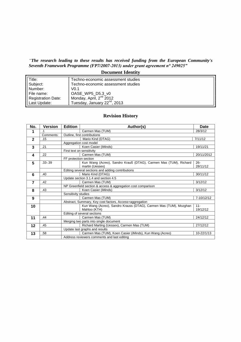
“The research leading to these results has received funding from the European Community's
Seventh Framework Programme (FP7/2007-2013) under grant agreement n° 249025”
Document Identity
Title: Techno-economic assessment studies Subject: Techno-economic assessment studies Number: V0.1 File name: OASE_WP5_D5.3_v0 Registration Date: Monday, April, 2
nd 2012
Last Update: Tuesday, January 22nd
, 2013
Revision History
No. Version Edition Author(s) Date
1 .1 Carmen Mas (TUM) 28/3/12
Comments: Outline, first contributions
2 .15 Mario Kind (DTAG) 7/11/12
Aggregation cost model
3 .21 Koen Casier (iMinds) 19/11/21
First text on sensitivity
4 .22 Carmen Mas (TUM) 20/11/2012
FF protection section
5 .33-.39 Kun Wang (Acreo), Sandro Krauß (DTAG), Carmen Mas (TUM), Richard martin (Uessex)
26-28/11/12
Editing several sections and adding contributions
6 .40 Mario Kind (DTAG) 30/11/12
Update section 3.1.4 and section 4.5
7 .42 Carmen Mas (TUM) 3/12/12
NP Greenfield section & access & aggregation cost comparison
8 .43 Koen Casier (iMinds) 3/12/12
Sensitivity studies
9 Carmen Mas (TUM) 7-10/12/12
Abstract, Summary, Key cost factors, Access+aggregation
10 Kun Wang (Acreo), Sandro Krauss (DTAG), Carmen Mas (TUM), Mozghan Mahloo (KTH)
11-19/12/12
Editing of several sections
11 .44 Carmen Mas (TUM) 24/12/12
Merging two parts into single document
12 .45 Richard Marting (Uessex), Carmen Mas (TUM) 27/12/12
Update last graphs and results
13 .58 Carmen Mas (TUM), Koen Casier (iMinds), Kun Wang (Acreo) 10-22/1/13
Address reviewers comments and last editing
Techno-economic assessment studies OASE_D5.3_WP5_TUM_220113v1.0
OASE FP7 – ICT– GA 249025
Page: 4 of 92
Table of Contents
EXECUTIVE SUMMARY ..................................................................................................................................... 6
REFERRED DOCUMENTS ................................................................................................................................. 8
LIST OF FIGURES AND TABLES...................................................................................................................... 9
ABBREVIATIONS .............................................................................................................................................. 12
1. INTRODUCTION ...................................................................................................................................... 14
2. TCO MODELLING .................................................................................................................................... 16
2.1. TCO BUILDING BLOCKS ...................................................................................................................... 16 2.2. DEMAND SCENARIO ............................................................................................................................ 17 2.3. AGGREGATION NETWORK MODEL ....................................................................................................... 18
3. CASE STUDIES ......................................................................................................................................... 20
3.1. NETWORK SCENARIOS ........................................................................................................................ 20 3.1.1. AREAS ................................................................................................................................................ 20 3.1.2. NODE CONSOLIDATION ....................................................................................................................... 20 3.1.3. PIP AND NP PENETRATION CURVES .................................................................................................... 21 3.1.4. DUCT AVAILABILITY IN FIRST MILE INFRASTRUCTURE SEGMENT ........................................................ 21 3.2. TECHNOLOGIES ................................................................................................................................... 22 3.2.1. GPON AND XGPON .......................................................................................................................... 22 3.2.2. AON HOMERUN AND ACTIVE STAR ..................................................................................................... 23 3.2.3. WAVELENGTH-ROUTED WDM PON (WR WDM PON) ..................................................................... 24 3.2.4. WAVELENGTH-SELECTIVE WDM PON (WS WDM PON) ................................................................. 25 3.2.5. UDWDM ........................................................................................................................................... 26 3.2.6. PASSIVE HYBRID PON ........................................................................................................................ 27 3.2.7. WDM PON BACKHAULING AON ....................................................................................................... 27 3.2.8. TWO-STAGE WDM PON .................................................................................................................... 28 3.3. PROTECTION SCENARIOS ..................................................................................................................... 28 3.3.1. FEEDER FIBRE PROTECTION ................................................................................................................ 28 3.3.2. DISTRIBUTION FIBRE PROTECTION ..................................................................................................... 29 3.4. OPEN ACCESS ..................................................................................................................................... 31
4. NGOA COST ASSESSMENT: MIGRATION: NP BROWNFIELD ....................................................... 33
4.1. INTRODUCTION: MIGRATION: NP BROWNFIELD ................................................................................. 33 4.1.1. MIGRATION SCENARIO – BASE ASSUMPTIONS ..................................................................................... 34 2.1.1. NGOA CUSTOMER MIGRATION ........................................................................................................... 35 4.2. COST ASSESSMENT ANALYSIS ............................................................................................................. 37 4.3. NGOA COST ASSESSMENT: NON-NODE CONSOLIDATION ................................................................... 40 4.3.1. DENSE URBAN AREA ........................................................................................................................... 40 4.3.2. RURAL AREA ....................................................................................................................................... 43 4.4. NGOA COST ASSESSMENT: AGGRESSIVE NODE CONSOLIDATION ....................................................... 46 4.4.1. DENSE URBAN AREA ........................................................................................................................... 47 4.4.2. RURAL AREA ....................................................................................................................................... 50 4.5. NON-NODE CONSOLIDATION VS. AGGRESSIVE NODE CONSOLIDATION ................................................ 54 4.6. IMPACT OF FEEDER FIBRE PROTECTION .............................................................................................. 56 4.6.1. DENSE URBAN AREA ........................................................................................................................... 56 4.6.2. RURAL AREA ....................................................................................................................................... 58
5. NGOA COST ASSESSMENT: MIGRATION: NP GREENFIELD ........................................................ 61
5.1. DENSE URBAN AREAS ......................................................................................................................... 61 5.2. RURAL AREAS ..................................................................................................................................... 62
6. NGOA COST ASSESSMENT: MIGRATION: PURE GREENFIELD ................................................... 64
7. FURTHER STUDIES ON “MIGRATION: NP BROWNFIELD” COST ASSESSMENT..................... 66
7.1. IDENTIFICATION OF COST KEY PARAMETERS ....................................................................................... 66
Techno-economic assessment studies OASE_D5.3_WP5_TUM_220113v1.0
OASE FP7 – ICT– GA 249025
Page: 5 of 92
7.2. COST EVALUATION OF THE EQUIPMENT PURELY USED FOR MIGRATION .............................................. 67 7.3. IMPACT OF MIGRATION TIME DURATION ON THE COST ASSESSMENT ................................................... 67 7.4. IMPACT OF MIGRATION STARTING TIME ON THE COST ASSESSMENT .................................................... 69
8. SENSITIVITY ANALYSIS ........................................................................................................................ 71
8.1. IMPACT OF LOOSENING THE OASE REQUIREMENTS ............................................................................ 72 8.2. REGIONAL DIFFERENCES .................................................................................................................... 75 8.3. IMPACT OF EQUIPMENT COSTS ............................................................................................................ 80 8.4. IMPACT OF ADOPTION RATE ................................................................................................................ 82
9. CONCLUSION AND GUIDELINES ........................................................................................................ 84
APPENDIX: URBAN COST ASSESSMENT ..................................................................................................... 86
APPENDIX B: ASSUMPTIONS OF COST ASSESSMENT ............................................................................ 92
Techno-economic assessment studies OASE_D5.3_WP5_TUM_220113v1.0
OASE FP7 – ICT– GA 249025
Page: 6 of 92
Executive summary
One of the objectives of the OASE project is to propose architectures able to guarantee the
requirements for next generation optical access networks. However, operators and
manufacturers are interested to evaluate the cost of each architecture in different scenarios and
to identify the cost drivers and key cost parameters.
Traditional optical access networks have been modelled based on the household concentration
of each area, which were classified as rural, urban and dense urban. However, operators are
playing with the possibility to change the scenario and reduce the number of central offices,
aiming at reducing costs, but also increasing the distance to users significantly and changing
the user distribution. The impact of the reduction of central offices, referred in this document
as node consolidation has been evaluated.
The cost evaluation is based on the extended TONIC tool, which has been implemented
within Task 5.2. The TONIC tool is able to dimension and evaluate cost of different
architectures (GPON, XGPON, Hybrid PON, WS WDM PON, WR WDM PON, AON +
WDM Backhaul) for different areas (dense urban, urban, rural) and different network
consolidation scenarios (non-node consolidation, conservative node consolidation, and
aggressive node consolidation). The dimensioning is done based on the selected penetration
curve (chosen among 7), the PIP penetration curve (either Greenfield in 2010 or in 2020) and
the assumed duct availability (5 available alternatives). The cost assessment comprises
infrastructure and equipment cost evaluation as well as fault management, service
provisioning, energy, floor space and maintenance required for each year based on the number
of connected users. Moreover, the tool is able to distinguish physical infrastructure provider
(PIP) costs from the network provider costs. The cost assessment considers the increase of
salaries and energy cost per year and provides non-discounted and discounted costs.
The proposed architectures are compared from the cost point of view under different
deployment assumptions:
- Migration from an existing traditional optical access network such as GPON or AON.
In this migration scenario, the investments in terms of infrastructure and equipment
are considered assuming an existing optical distribution network (ODN). This ODN
can be used for the NGOA from the migration starting time on.
The cost assessment shows that for all the architectures have higher OPEX than
CAPEX costs when summing the costs from 2020 to 2030 (NGOA operational time)
for any type of area (i.e. DU, U and R). The most costly architecture is the UDWDM
for any area, whereas the less costly solutions is to keep existing optical access
networks: upgrade existing GPON by reducing the splitting ration from 32 to 8 so that
the bandwidth increases or to keep the AON as it is. The CAPEX key cost factors of
these architectures differ: for UDWDM is NP and CPE equipment, for AON is the NP
equipment and in-house infrastructure, whereas for the GPON upgrade is CPE and in-
house infrastructure. Regarding OPEX, the most important factor is the service
provisioning. The impact of energy and FM differs significantly on the architecture
(e.g. UDWDM has high energy and FM but relatively low CPE energy cost; AON has
Techno-economic assessment studies OASE_D5.3_WP5_TUM_220113v1.0
OASE FP7 – ICT– GA 249025
Page: 7 of 92
low CPE related costs; whereas GPON has lower values but slightly higher CPE
energy cost).
When considering node consolidation, more architectures have been evaluated since
they can offer the long reach requirements while keeping the high bandwidth per user.
In this scenario, it can be observed that the upgrade of GPON by reducing the splitting
ratio is not an option due to the high costs related to the new LL5 links (increases
more than 1 CU/year per user). Some architectures keep and even decrease their
average TCO per user per year when applied to aggressive node consolidation
scenarios: e.g. HPON40 (for any area) and WSWDM PON (for DU) solutions.
Furthermore, the options to connect AON AS with a WDM Backhaul, or migrate from
GPON to HPON architecture are the most effective solutions for any type of area
applying node consolidation.
- Migration from a non-optical access network towards an NGOA. This migration
scenario considers a network provider greenfield scenario where some ducts can be
used to install the optical fiber. The impact of an NP greenfield is mostly on the
increase of service provisioning costs due to the higher effort required to connect all
users, as well as on the infrastructure cost (especially in rural areas where the distances
are significantly longer).
- The impact of the ducts availability on the total cost is given by comparing the
previous results with a pure greenfield scenario as well as with a higher availability
scenario. The impact of duct availability on the infrastructure cost differs on the
architecture and on the area: higher for DU than rural areas, higher for AON P2P and
WRWDM PON than HPON solutions.
- A higher fanout will for all architectures lead to a lower cost per home passed and to a
lower overall cost. Cost reductions up to 30% and more are reachable by increasing
the fanout substantially. It should be noted that the higher fanout cases might conflict
with the consolidation possibilities – as a higher fanout will reduce the reach – and
maximum dedicated bandwidth – as with a higher fanout, more customers are sharing
the same OLT port. Relaxing the OASE requirements – for instance only in an initial
phase – could as such reduce the upfront costs substantially
- Regional differences could lead to a very different cost of deployment. Especially in
those European countries with lower average salaries, the costs could be much lower.
Next to the salary, the adoption is the most important impacting factor and a higher
adoption will lead to a lower cost per customer in the end.
- The impact of costs of the ONT and OLT equipment behaves more or less linear for
all architectures and has a rather limited impact up to resp. ~5% or ~2% for an
increase up to 50% of its original cost.
- Adoption has most probably the highest impact of all factors and has been split into
initial adoption effect (e.g. by means of presubscriptions) and the steepness of the
adoption curve. Increases in the initial adoption lead to the most substantial decrease
in the cost per subscription year. Still the effect of having a faster adoption is certainly
very important
Techno-economic assessment studies OASE_D5.3_WP5_TUM_220113v1.0
OASE FP7 – ICT– GA 249025
Page: 8 of 92
Referred documents
[1] OASE Deliverable D2.2 “Consolidated requirements for European next-generation optical
access networks” June 2012
[2] OASE Deliverable D5.2 “Process modeling and first version of TCO evaluation tool”
December 2011
[3] OASE Deliverable D5.1 “Overview of Methods and Tools” October 2010.
[4] OASE Deliverable D6.3 “Value network evaluation” December 2012
[5] OASE Deliverable D3.2 “Description and assessment of the architecture options”
September 2012
[6] OASE Deliverable D4.2.2 “Technical assessment and comparison of next-generation
optical access system concepts” March 2012
[7] OASE Deliverable D6.2 “Market Demands and Revenues” June 2012.
Techno-economic assessment studies OASE_D5.3_WP5_TUM_220113v1.0
OASE FP7 – ICT– GA 249025
Page: 9 of 92
List of figures and tables
Figure 1 Overview of the required TCO input data ................................................................. 14 Figure 2 Building blocks of the TCO model ............................................................................ 16 Figure 3 Penetration evolution ................................................................................................. 17 Figure 4 Evolution of sustainable traffic per user .................................................................... 18 Figure 5 Aggregation cost model ............................................................................................. 19
Figure 6 Non-node consolidation reaches up to the local exchange (PCP5), whereas node
consolidation reaches the central access node (PCP6) ............................................................. 20 Figure 7 Network Provider (NP) penetration curves ............................................................... 21 Figure 8 OASE considered NGOA technologies ..................................................................... 22 Figure 9 GPON architecture ..................................................................................................... 23
Figure 10 AON P2P, reference scenario, non-node consolidation .......................................... 23
Figure 11 AON active star, reference scenario, non-node consolidation ................................. 24 Figure 12 AON active star with extensive use of the aggregation network. ............................ 24
Figure 13 Wavelength Routed WDM-PON architecture ......................................................... 25 Figure 14 Tunable-based WS-WDM-PON: assignment to PCP sites (D4.2.2 [6]) ................. 25 Figure 15 The UDWDM System Concept ............................................................................... 26
Figure 16 HPON architecture in case of node consolidation ................................................... 27 Figure 17 WDM PON backhauling AON ................................................................................ 27 Figure 18 Two-stage WDM PON ............................................................................................ 28
Figure 19 Feeder Fiber (FF) protection for HPON architecture .............................................. 29 Figure 20 Additional trenching required on top of the original structure in order to get a fully
resilient network. ...................................................................................................................... 30 Figure 21 Detailed view of the upper half of the resiliency structure for evaluating the
analytical calculation structure and formula. ........................................................................... 30
Figure 22 Additional cost estimated for installation of a fully resilient distribution network as
a factor of the size (in customers) of each separated distribution section. ............................... 31 Figure 23 Considered general migration steps ......................................................................... 34 Figure 24 Example HPON migration versus GPON reference in node consolidation ........... 35
Figure 25 WP6 likely penetration evolution and migration numbers ..................................... 36
Figure 26 Non discounted TCO in DU area ............................................................................. 40 Figure 27 Total CAPEX [CU] on the left axis and CAPEX per user [CU/user] on the right
axis of different NGOAs in Dense Urban area with non-node consolidation .......................... 41 Figure 28 Total OPEX [CU] (left axis) and OPEX per user (right axis) in Dense Urban areas
with non-node consolidation .................................................................................................... 41
Figure 29 Non discounted TCO [CU] per year in DU areas with non-node consolidation ..... 42 Figure 30 Discounted TCO [CU] per year in DU areas with non-node consolidation ............ 42 Figure 31 Average non discounted TCO (CAPEX components in blue and OPEX
components in red) per connected user per year in DU areas .................................................. 43 Figure 32 Non discounted TCO in rural area ........................................................................... 44 Figure 33 CAPEX [CU] on the left axis and CAPEX per user [CU/user] on the right axis of
different NGOAs in rural areas with non-node consolidation ................................................. 44
Figure 34 Total OPEX [CU] (left axis) and OPEX per user (right axis) in rural areas with non-
node consolidation .................................................................................................................... 45 Figure 35 TCO [CU] per year in rural areas with non-node consolidation .............................. 45 Figure 36 Discounted TCO [CU] in rural areas with non-node consolidation ........................ 46 Figure 37 Average non discounted TCO (CAPEX components in blue and OPEX components
in red) per connected user per year in rural areas .................................................................... 46
Techno-economic assessment studies OASE_D5.3_WP5_TUM_220113v1.0
OASE FP7 – ICT– GA 249025
Page: 10 of 92
Figure 38 Non discounted TCO in DU with aggressive node consolidation ........................... 47
Figure 39 CAPEX [CU] on the left axis and CAPEX per user [CU/user] on the right axis of
different NGOAs in dense urban areas with aggressive node consolidation ........................... 48 Figure 40 OPEX [CU] (left axis) and OPEX per user [CU/user] (right axis) of different
NGOA solutions in dense urban areas with aggressive node consolidation ............................ 49 Figure 41 Non discounted TCO [CU] per year in DU areas aggressive consolidation scenario
.................................................................................................................................................. 49 Figure 42 Discounted TCO [CU] per year in DU areas aggressive consolidation scenario .... 50 Figure 43 Average non discounted TCO per connected user per year ..................................... 50
Figure 44 Non discounted TCO in rural areas with aggressive node consolidation ................ 51 Figure 45 CAPEX [CU] on the left axis and CAPEX per user [CU/user] on the right axis of
different NGOAs in rural areas with aggressive node consolidation ....................................... 52 Figure 46 Total OPEX [CU] (left axis) and OPEX per user [CU/user] (right axis) of different
NGOA solutions in rural areas with aggressive node consolidation scenario ......................... 52
Figure 47 TCO [CU] per year in Rural areas with aggressive consolidation scenario ............ 53 Figure 48 Discounted TCO [CU] in Rural areas with aggressive node consolidation ............ 53
Figure 49 Average non discounted TCO per connected user per year for Rural areas ............ 54 Figure 50 Access NP and aggregation cost per user [CU/user] for active and passive
architectures with and without node consolidation .................................................................. 55 Figure 51 Cost per user [CU/user] savings when implementing node consolidation .............. 55
Figure 52 Increase of CAPEX when offering FF protection ................................................... 57 Figure 53 Increase of accumulated OPEX when offering FF protection ................................. 57 Figure 54 TCO for unprotected and FF protected solutions in DU areas ................................ 58
Figure 55 Increase of CAPEX when offering FF protection in Rural areas ............................ 59 Figure 56 Increase of OPEX when offering FF protection in rural areas ................................ 59
Figure 57 TCO for unprotected and FF protected solutions in rural areas .............................. 60 Figure 58 NP Greenfield: Total CAPEX for DU areas ............................................................ 61
Figure 59 NP Greenfield: Total OPEX for DU areas ............................................................... 62 Figure 60 NP Greenfield: Total CAPEX for rural areas .......................................................... 62
Figure 61 NP Greenfield: Total OPEX for rural areas ............................................................. 63 Figure 62 Non-node consolidation: Infrastructure cost of different architectures taking into
account different duct availability assumptions: Greenfield "GF", partial "S" and extended
"XL" ......................................................................................................................................... 64 Figure 63 Aggressive node consolidation: Infrastructure costs of different architectures for
different duct availability degrees: "GF", "S" and "XL" (refer to Section 3.1.4 ). .................. 65 Figure 64 Cost evolution for 1 (top) and 3 (bottom) year migration duration ......................... 68 Figure 65 Cost evolution for migration starting in 2020 (top) or 2023 (bottom) ..................... 69 Figure 66: Cumulative non discounted cost as a function of the fanout, averaged over all
variations in a 7500 node consolidation scenario ..................................................................... 73
Figure 67: Cumulative non discounted cost as a function of the fanout, averaged over all
variations in a 1000 node consolidation scenario ..................................................................... 74
Figure 68 Increase in average costs of different architectures in function of fanout and relative
to the average cost of GPON 64 (asymptotical minimum) ...................................................... 74 Figure 69: cumulative costs over the period 2020-2030 for the different architectures and
regions with relation to the OASE project. (Top) Total cumulative (Bottom) relative to
HPON40-1:32 ........................................................................................................................... 77
Figure 70: cumulative costs over the period 2020-2030 for the different architectures and
regions with relation to the OASE project (Top) Total Cumulative (Bottom) relative to the
base case TONIC ...................................................................................................................... 78
Techno-economic assessment studies OASE_D5.3_WP5_TUM_220113v1.0
OASE FP7 – ICT– GA 249025
Page: 11 of 92
Figure 71: costs per subscription year over the period 2020-2030 for the different
architectures and regions with relation to the OASE project. .................................................. 79 Figure 72: impact of the cost per customer for differences in CPE cost, relative on a per
architecture basis to the situation with the original CPE cost. ................................................. 80
Figure 73: impact of the cost per customer for differences in OLT cost, relative on a per
architecture basis to the situation with the original OLT cost.................................................. 81 Figure 74 Expected revenues per subscription to reach breakeven PIP+NP ........................... 82 Figure 75 Expected revenues per subscription to reach breakeven PIP (left) and NP (right) .. 82 Figure 76 Expected subscription rate scaling to the initial adoption rate (left) and adoption
rate (right) ................................................................................................................................. 83 Figure 78 Non discounted TCO in urban areas (non-node consolidation) .............................. 86 Figure 79 Total CAPEX [CU] of the left axis and CAPEX per user [CU/user] on the right axis
of different NGOAs in urban area with non-node consolidation ............................................. 86 Figure 80 Total OPEX [CU] (left axis) and OPEX per user (right axis) in urban areas with
non-node consolidation ............................................................................................................ 87 Figure 81 Non discounted TCO [CU] per year in urban areas with non node consolidation .. 87
Figure 82 Discounted TCO[CU] per year in urban areas with non-node consolidation .......... 88 Figure 83 Average TCO (CAPEX components in blue and OPEX components in red) per
connected user per year in urban areas) ................................................................................... 88 Figure 84 Non discounted TCO for urban areas with aggressive node consolidation ............. 89
Figure 85 Total CAPEX [CU] of the left axis and CAPEX per user [CU/user] on the right axis
of different NGOAs in urban area with aggressive node consolidation .................................. 89 Figure 86 Total OPEX [CU] of the left axis and OPEX per user [CU/user] on the right axis of
different NGOAs in urban area with aggressive node consolidation ....................................... 90 Figure 87 Non discounted TCO [CU] per year in urban areas with aggressive node
consolidation ............................................................................................................................ 90 Figure 88 Discounted TCO [CU] per year in urban areas with aggressive node consolidation
.................................................................................................................................................. 91 Figure 89 Average TCO (CAPEX components in blue and OPEX components in red) per
connected user per year in urban areas). .................................................................................. 91
Table 1 Evaluated NGOA architectures ................................................................................... 33 Table 2 Migration specific efforts per architecture .................................................................. 36 Table 3 TCO cost in 2010 for the different scenarios .............................................................. 37 Table 4 Key cost factors (as % of the TCO) in the aggressive node consolidation scenario ... 66
Table 5 Key cost factors in the non-node consolidation scenario ............................................ 67 Table 6 Migration dedicated equipment cost [CU] .................................................................. 67 Table 7 Sum of costs 2020-2030 when the duration of the migration is one and three years.. 68
Table 8 Sum of costs 2020-2030 when starting the migration in 2020 and in 2023 ................ 70 Table 9: Set of parameters influenced by the regional differences, applied to the set of
considered regions and their extremes ..................................................................................... 75 Table 10: Reduced set of parameters for the regional differences which can be used directly in
TONIC and have been related to the original values in TONIC. ............................................. 76
Techno-economic assessment studies OASE_D5.3_WP5_TUM_220113v1.0
OASE FP7 – ICT– GA 249025
Page: 12 of 92
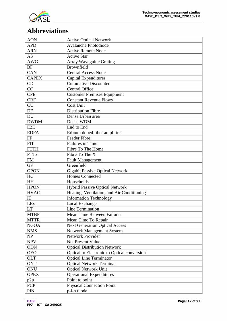
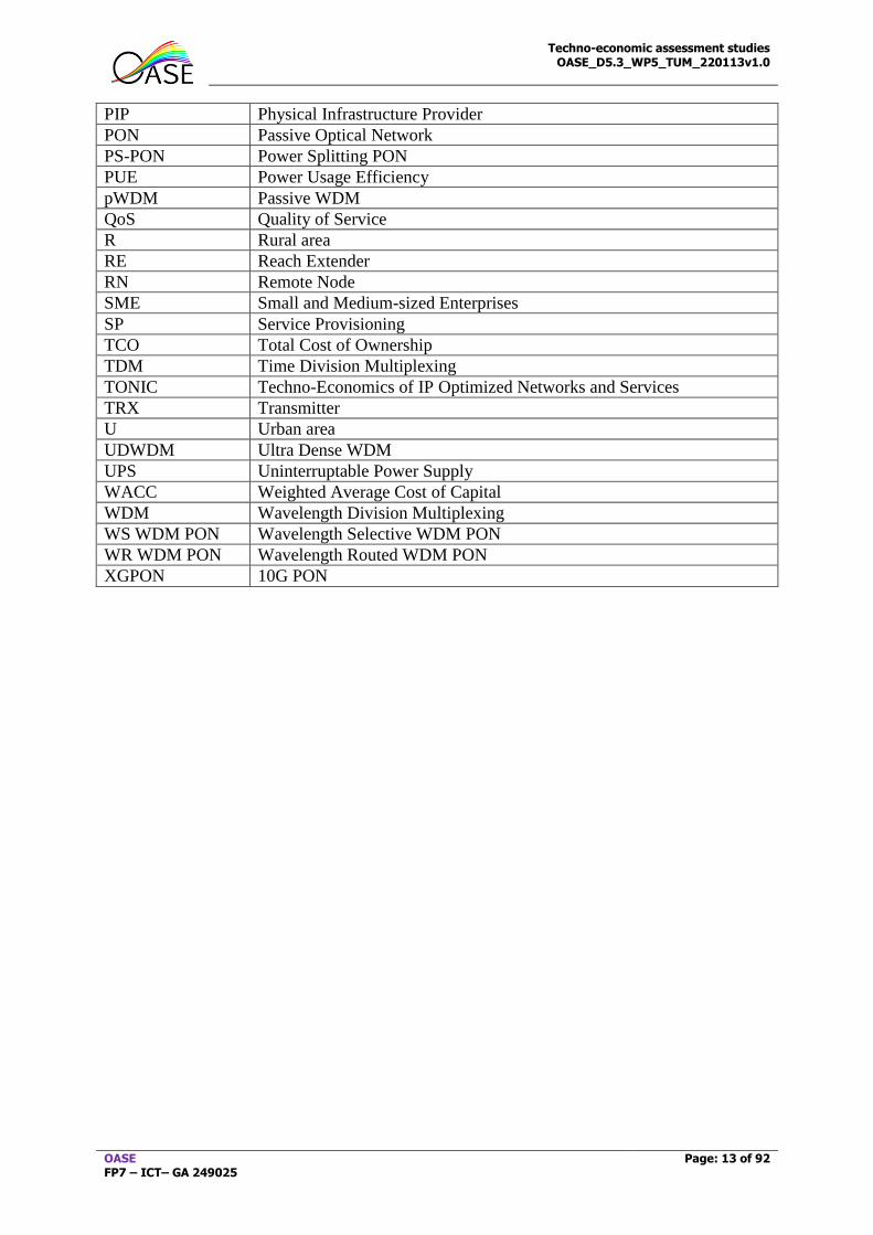
Abbreviations
AON Active Optical Network APD Avalanche Photodiode
ARN Active Remote Node
AS Active Star
AWG Array Waveguide Grating
BF Brownfield
CAN Central Access Node
CAPEX Capital Expenditures
CD Cumulative Discounted
CO Central Office
CPE Customer Premises Equipment
CRF Constant Revenue Flows
CU Cost Unit
DF Distribution Fibre
DU Dense Urban area
DWDM Dense WDM
E2E End to End
EDFA Erbium doped fiber amplifier
FF Feeder Fibre
FIT Failures in Time
FTTH Fibre To The Home
FTTx Fibre To The X
FM Fault Management
GF Greenfield
GPON Gigabit Passive Optical Network
HC Homes Connected
HH Households
HPON Hybrid Passive Optical Network
HVAC Heating, Ventilation, and Air Conditioning
IT Information Technology
LEx Local Exchange
LT Line Termination
MTBF Mean Time Between Failures
MTTR Mean Time To Repair
NGOA Next Generation Optical Access
NMS Network Management System
NP Network Provider
NPV Net Present Value
ODN Optical Distribution Network
OEO Optical to Electronic to Optical conversion
OLT Optical Line Terminator
ONT Optical Network Terminal
ONU Optical Network Unit
OPEX Operational Expenditures
p2p Point to point
PCP Physical Connection Point
PIN p-i-n diode
Techno-economic assessment studies OASE_D5.3_WP5_TUM_220113v1.0
OASE FP7 – ICT– GA 249025
Page: 13 of 92
PIP Physical Infrastructure Provider
PON Passive Optical Network
PS-PON Power Splitting PON
PUE Power Usage Efficiency
pWDM Passive WDM
QoS Quality of Service
R Rural area
RE Reach Extender
RN Remote Node
SME Small and Medium-sized Enterprises
SP Service Provisioning
TCO Total Cost of Ownership
TDM Time Division Multiplexing
TONIC Techno-Economics of IP Optimized Networks and Services
TRX Transmitter
U Urban area
UDWDM Ultra Dense WDM
UPS Uninterruptable Power Supply
WACC Weighted Average Cost of Capital
WDM Wavelength Division Multiplexing
WS WDM PON Wavelength Selective WDM PON
WR WDM PON Wavelength Routed WDM PON
XGPON 10G PON
Techno-economic assessment studies OASE_D5.3_WP5_TUM_220113v1.0
OASE FP7 – ICT– GA 249025
Page: 14 of 92
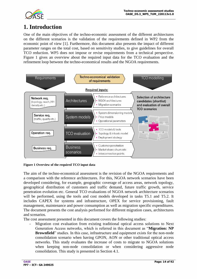
1. Introduction
One of the main objectives of the techno-economic assessment of the different architectures
on the different scenarios is the validation of the requirements defined in WP2 from the
economic point of view [1]. Furthermore, this document also presents the impact of different
parameter ranges on the total cost, based on sensitivity studies, to give guidelines for overall
TCO reduction. WP5 does not impose or revise requirements from a technical perspective.
Figure 1 gives an overview about the required input data for the TCO evaluation and the
refinement loop between the techno-economical results and the NGOA requirements.
Figure 1 Overview of the required TCO input data
The aim of the techno-economical assessment is the revision of the NGOA requirements and
a comparison with the reference architectures. For this, NGOA network scenarios have been
developed considering, for example, geographic coverage of access areas, network topology,
geographical distribution of customers and traffic demand, future traffic growth, service
penetration evolution etc. General TCO evaluations of NGOA network architecture scenarios
will be performed, using the tools and cost models developed in tasks T5.1 and T5.2. It
includes CAPEX for systems and infrastructure, OPEX for service provisioning, fault
management, maintenance and power consumption as well as migration specific expenditures.
The document presents the cost analysis performed for different migration cases, architectures
and scenarios.
The cost assessment presented in this document covers the following studies:
- Migration cost evaluation from existing traditional optical access solutions to Next
Generation Access networks, which is referred in this document as “Migration: NP
Brownfield” studies. In this case, infrastructure and equipment exists for the non-node
consolidation scenario when having GPON, AON or other traditional optical access
networks. This study evaluates the increase of costs to migrate to NGOA solutions
when keeping non-node consolidation or when considering aggressive node
consolidation. This study is presented in Section 4.1.
Techno-economic assessment studies OASE_D5.3_WP5_TUM_220113v1.0
OASE FP7 – ICT– GA 249025
Page: 15 of 92
- Migration cost evaluation from non-optical access networks (e.g. copper network)
where some ducts may be available to be used by optical cables. This case is referred
as “NP Greenfield” and is presented in Section 4.2.
- Furthermore, it may require the cost evaluation from a pure Greenfield scenario, that
is, no NP or PIP available. The cost difference of this solution versus the “NP
Greenfield” is presented in Section 4.3.
The impact of some aspects such as migration duration, protection, and migration starting
time, is also stated. Furthermore a complete sensitivity analysis showing the impact that the
variation of some parameters (due to regional location, time dependence or wrong
estimations) have on the cost assessment is also provided in this deliverable.
The cost assessment also aims at identifying the key cost drivers and evaluating the impact
that different input parameters and the targeted European region will have on the results.
The document is structured as follows: Section 1 provides a general description. In Section 2
the general cost model is described. Section 3 presents the case studies in terms of network
scenarios (including type of area, node aggregation degree, penetration curves and duct
availability), technologies, protection and open access. Section 4 presents the whole cost
assessment for the different migration cases. In Section 5 some more specific cost studies are
presented, which includes the impact of protection on the cost, cost evaluation of specific
equipment required for the migration or the impact of the migration duration on the cost.
Section 6 is devoted to all the sensitivity studies performed such as the impact that regional
parameters have on the cost assessment. Finally Section 7 concludes the deliverable.
Techno-economic assessment studies OASE_D5.3_WP5_TUM_220113v1.0
OASE FP7 – ICT– GA 249025
Page: 16 of 92
2. TCO Modelling
This section gives an overview of the relevant input parameters and boundary conditions of
the study, comprising TCO building blocks, deployment conditions, demand scenario and
aggregation cost model.
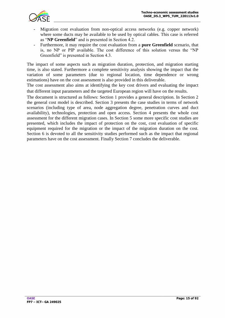
2.1. TCO building blocks
The TCO model comprises investments for all active and passive system and infrastructure
components, expenditures for network operations and location infrastructure as well as
migration related cost. Figure 2 shows the considered building blocks of the TCO model,
which is based on the process modelling, proposed in D5.2 [2].
Figure 2 Building blocks of the TCO model
The business case has a time horizon for the NGOA deployment and operation from 2020-
2030. For simplification, 100% of the FTTH network basic rollout has been considered in the
first deployment year, even if this does probably not reflect the reality of what is likely to
occur. No significant difference is expected for the system architecture comparison as
compared to a delayed deployment, e.g. by over 3 years. In order to cover the varying
infrastructure and topology requirements (e.g. available ducts, reach etc.) of different access
areas, three Geo-type clusters: Dense Urban, Urban and Rural have been compared. The TCO
modelling is performed for one typical/traditional service access area of each Geo-cluster. The
passive fibre infrastructure deployment of the PIP takes into account existing free duct
infrastructure (Brownfield), but no potentially existing spare fibres. For the NGOA system
deployment of the NP, a Greenfield scenario in areas without existing FTTH and a migration
scenario in areas with existing FTTH deployment (e.g. GPON or P2P) have been evaluated.
In the migration scenarios, two FTTH initial architectures are considered from 2010-2019, in
Techno-economic assessment studies OASE_D5.3_WP5_TUM_220113v1.0
OASE FP7 – ICT– GA 249025
Page: 17 of 92
order to cover the upfront ODN deployment cost and to estimate the proper migration start
point in 2019/20.
2.2. Demand scenario
Major drivers for optical network deployments are market demands and competition. The
network design and dimensioning depends primary on the evolution forecast of service
penetration and sustainable traffic per user as well as the requested access peak bandwidths.
These dimensioning parameters are basically influenced by the offered service portfolio and
competition situation in an access area.
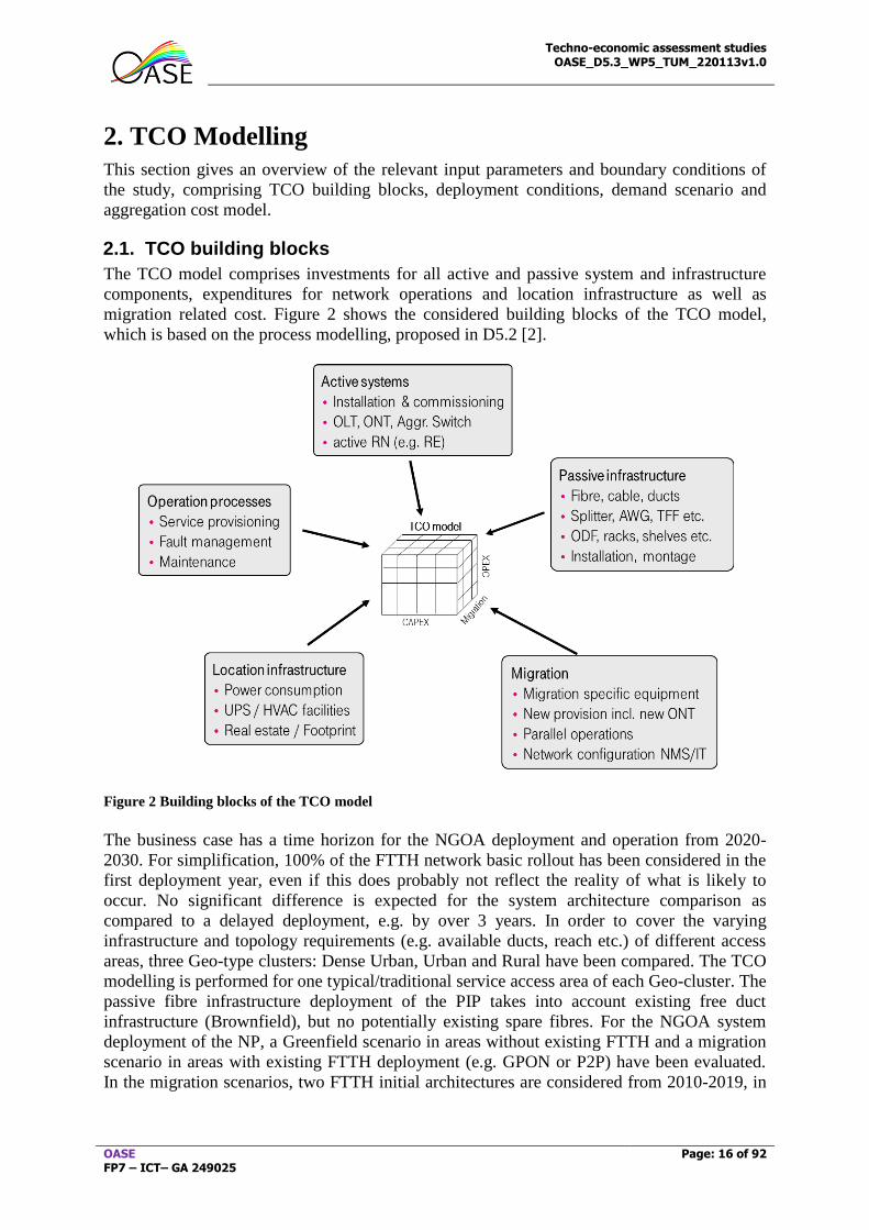
Figure 3 shows an example penetration forecast for Germany for a time horizon till 2030,
obtained from WP6. It reflects the average FTTH penetration of all deployed access areas.
The migration strategy may depend on the reached penetration level in the migration start
year (e.g. in 2020). In case of a relatively low customer penetration in 2020 on the existing
FTTH platform, a “forced” migration with a completely switchover of all existing customers
may come in the game instead of an “overlay” migration over several years in order to avoid
parallel platform operations.
Figure 3 Penetration evolution
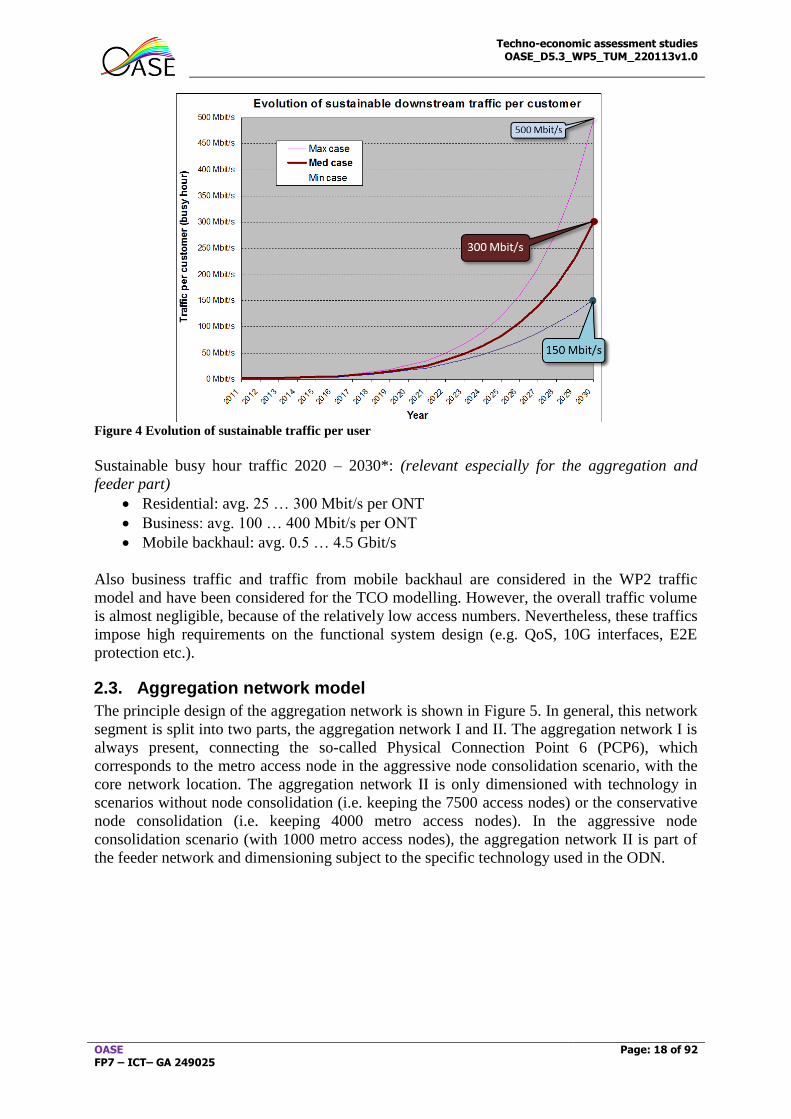
Figure 4 shows the WP2 requirement on the evolution of the sustainable traffic per customer.
A Medium traffic case with 300 Mbit/s per customer (in 2030) has been considered out of the
spanned traffic corridor for the TCO base scenarios. The sustainable traffic evolution is
especially relevant for the aggregation and OLT switch dimensioning and in TDM based
architectures also for the feeder dimensioning. The Max traffic case determines the system
minimum requirement (i.e. NGOA systems have to support it) and will be considered as a
sensitivity study.
Peak access bandwidths:
Residential: 1G per ONT
Business: 70% 1G and 30% 10G per ONT
Mobile backhaul: 10G per Base station
Techno-economic assessment studies OASE_D5.3_WP5_TUM_220113v1.0
OASE FP7 – ICT– GA 249025
Page: 18 of 92
Figure 4 Evolution of sustainable traffic per user
Sustainable busy hour traffic 2020 – 2030*: (relevant especially for the aggregation and
feeder part)
Residential: avg. 25 … 300 Mbit/s per ONT
Business: avg. 100 … 400 Mbit/s per ONT
Mobile backhaul: avg. 0.5 … 4.5 Gbit/s
Also business traffic and traffic from mobile backhaul are considered in the WP2 traffic
model and have been considered for the TCO modelling. However, the overall traffic volume
is almost negligible, because of the relatively low access numbers. Nevertheless, these traffics
impose high requirements on the functional system design (e.g. QoS, 10G interfaces, E2E
protection etc.).
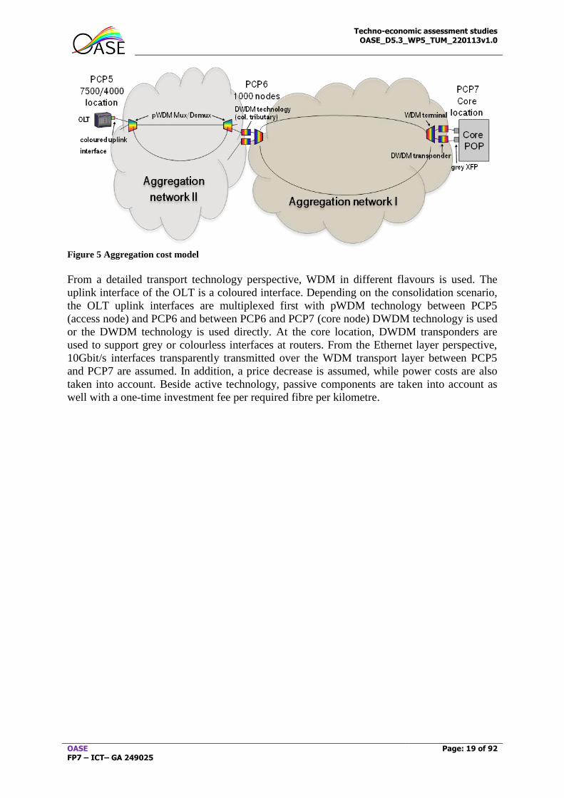
2.3. Aggregation network model
The principle design of the aggregation network is shown in Figure 5. In general, this network
segment is split into two parts, the aggregation network I and II. The aggregation network I is
always present, connecting the so-called Physical Connection Point 6 (PCP6), which
corresponds to the metro access node in the aggressive node consolidation scenario, with the
core network location. The aggregation network II is only dimensioned with technology in
scenarios without node consolidation (i.e. keeping the 7500 access nodes) or the conservative
node consolidation (i.e. keeping 4000 metro access nodes). In the aggressive node
consolidation scenario (with 1000 metro access nodes), the aggregation network II is part of
the feeder network and dimensioning subject to the specific technology used in the ODN.
Techno-economic assessment studies OASE_D5.3_WP5_TUM_220113v1.0
OASE FP7 – ICT– GA 249025
Page: 19 of 92
Figure 5 Aggregation cost model
From a detailed transport technology perspective, WDM in different flavours is used. The
uplink interface of the OLT is a coloured interface. Depending on the consolidation scenario,
the OLT uplink interfaces are multiplexed first with pWDM technology between PCP5
(access node) and PCP6 and between PCP6 and PCP7 (core node) DWDM technology is used
or the DWDM technology is used directly. At the core location, DWDM transponders are
used to support grey or colourless interfaces at routers. From the Ethernet layer perspective,
10Gbit/s interfaces transparently transmitted over the WDM transport layer between PCP5
and PCP7 are assumed. In addition, a price decrease is assumed, while power costs are also
taken into account. Beside active technology, passive components are taken into account as
well with a one-time investment fee per required fibre per kilometre.
Techno-economic assessment studies OASE_D5.3_WP5_TUM_220113v1.0
OASE FP7 – ICT– GA 249025
Page: 20 of 92
3. Case Studies
This section introduces the characteristics defining each case study of the cost assessment,
which are:
Network scenario: Area, node consolidation degree, penetration curve and duct availability
Technology
Protection (Feeder fibre or end-to-end protection)
Open Access
3.1. Network scenarios
3.1.1. Areas
In OASE, three types of area have been studied as proposed in Deliverable D5.1 [3]:
Dense Urban areas: these are the most populated areas that have thousands of
households per square kilometre.
Urban areas: these areas have an average of hundreds of households per square
kilometre.
Rural areas are the less populated areas with tens of households per square kilometre.
Any area or region of Europe can be associated to one of these three areas depending on the
household density.
3.1.2. Node consolidation
As introduced in D5.1 [3], traditional access areas (whose central office is referred as access
node) can be grouped into larger areas so that the total number of central offices can be
reduced, expecting also a reduction of the associated costs. The larger areas tend to be called
NGOA service areas, and their central offices are labelled as metro access nodes.
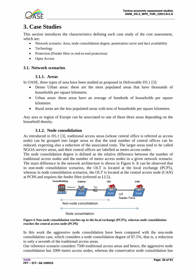
The node consolidation degree is defined as the relative difference between the number of
traditional access nodes and the number of metro access nodes in a given network scenario.
The main difference in the network architecture is shown in Figure 6. It can be observed that
in non-node consolidation scenarios, the OLT is located at the local exchange (PCP5),
whereas in node consolidation scenarios, the OLT is located at the central access node (CAN)
at PCP6 and requires the feeder fibre (referred as LL5).
Figure 6 Non-node consolidation reaches up to the local exchange (PCP5), whereas node consolidation
reaches the central access node (PCP6)
In this work the aggressive node consolidation have been compared with the non-node
consolidation case, which considers a node consolidation degree of 87.5%, that is, a reduction
to only a seventh of the traditional access areas.
Our reference scenario considers 7500 traditional access areas and hence, the aggressive node
consolidation has 1000 metro access nodes, whereas the conservative node consolidation has
Techno-economic assessment studies OASE_D5.3_WP5_TUM_220113v1.0
OASE FP7 – ICT– GA 249025
Page: 21 of 92
4000 metro access nodes. However, any area of Europe can be mapped to one of these
scenarios, which were described in D5.1 [3].
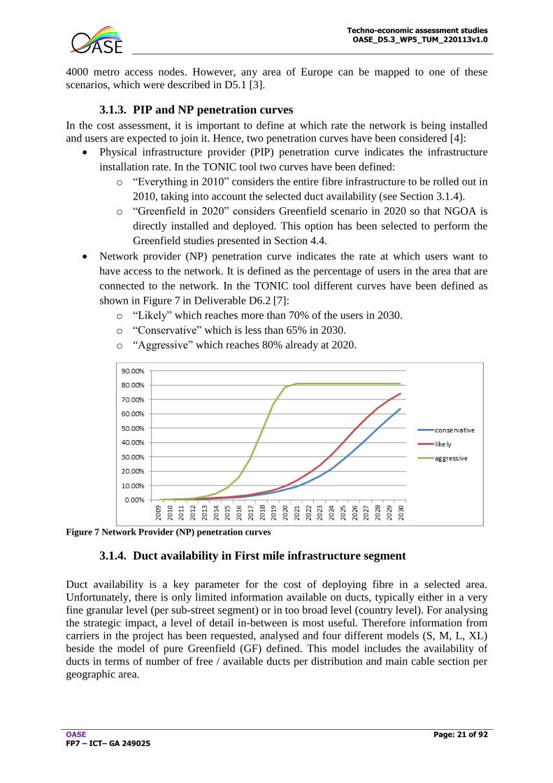
3.1.3. PIP and NP penetration curves
In the cost assessment, it is important to define at which rate the network is being installed
and users are expected to join it. Hence, two penetration curves have been considered [4]:
Physical infrastructure provider (PIP) penetration curve indicates the infrastructure
installation rate. In the TONIC tool two curves have been defined:
o “Everything in 2010” considers the entire fibre infrastructure to be rolled out in
2010, taking into account the selected duct availability (see Section 3.1.4).
o “Greenfield in 2020” considers Greenfield scenario in 2020 so that NGOA is
directly installed and deployed. This option has been selected to perform the
Greenfield studies presented in Section 4.4.
Network provider (NP) penetration curve indicates the rate at which users want to
have access to the network. It is defined as the percentage of users in the area that are
connected to the network. In the TONIC tool different curves have been defined as
shown in Figure 7 in Deliverable D6.2 [7]:
o “Likely” which reaches more than 70% of the users in 2030.
o “Conservative” which is less than 65% in 2030.
o “Aggressive” which reaches 80% already at 2020.
Figure 7 Network Provider (NP) penetration curves
3.1.4. Duct availability in First mile infrastructure segment
Duct availability is a key parameter for the cost of deploying fibre in a selected area.
Unfortunately, there is only limited information available on ducts, typically either in a very
fine granular level (per sub-street segment) or in too broad level (country level). For analysing
the strategic impact, a level of detail in-between is most useful. Therefore information from
carriers in the project has been requested, analysed and four different models (S, M, L, XL)
beside the model of pure Greenfield (GF) defined. This model includes the availability of
ducts in terms of number of free / available ducts per distribution and main cable section per
geographic area.
Techno-economic assessment studies OASE_D5.3_WP5_TUM_220113v1.0
OASE FP7 – ICT– GA 249025
Page: 22 of 92
Overall 15 different parameter combinations for the areas exist, but the analysis is limited to
the brownfield scenarios “S” (small duct space availability) and “XL” (extra-large duct space
availability) reflecting some kind of extreme case analysis and pure Greenfield as the
potential upper end of costs. Some basic information on the scenarios:
“Greenfield”: as the name indicates, it corresponds to the Greenfield scenario where
no duct is available and hence, all infrastructures should be installed.
“S” refers to the brownfield scenario (it corresponds to the “-“ option of Figure 23 in
D5.2 [1]). In this scenario, only a limited percentage of ducts (between 1 and 3 empty
ducts) is available (main cable section between 50% in dense urban, 28% in urban and
10% in rural; distribution cable section between 12% for dense urban, 8% in urban and
1% in rural).
“XL” refers to the brownfield scenario (it corresponds to the “++“ option of Figure 23
in D5.2). In this scenario, a high percentage of ducts (between 1 and 3 empty ducts) is
available (main cable section between 94% in dense urban, 73% in urban and 55% in
rural; distribution cable section between 70% for dense urban, 30% in urban and 15%
in rural).
More details on the different models are presented in Section 4.1 of D5.2 [1].
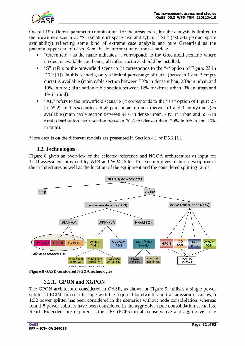
3.2. Technologies
Figure 8 gives an overview of the selected reference and NGOA architectures as input for
TCO assessment provided by WP3 and WP4 [5,6]. This section gives a short description of
the architectures as well as the location of the equipment and the considered splitting ratios.
Figure 8 OASE considered NGOA technologies
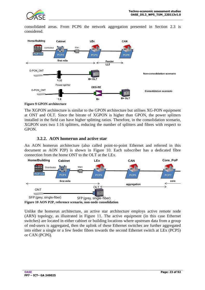
3.2.1. GPON and XGPON
The GPON architecture considered in OASE, as shown in Figure 9, utilises a single power
splitter at PCP4. In order to cope with the required bandwidth and transmission distances, a
1:32 power splitter has been considered in the scenarios without node consolidation, whereas
four 1:8 power splitters have been considered in the aggressive node consolidation scenarios.
Reach Extenders are required at the LEx (PCP5) in all conservative and aggressive node
Techno-economic assessment studies OASE_D5.3_WP5_TUM_220113v1.0
OASE FP7 – ICT– GA 249025
Page: 23 of 92
consolidated areas. From PCP6 the network aggregation presented in Section 2.3 is
considered.
Figure 9 GPON architecture
The XGPON architecture is similar to the GPON architecture but utilises XG-PON equipment
at ONT and OLT. Since the bitrate of XGPON is higher than GPON, the power splitters
installed in the field can have higher splitting ratios. Therefore, in the consolidation scenario,
XGPON uses two 1:16 splitters, reducing the number of splitters and fibres with respect to
GPON.
3.2.2. AON homerun and active star
An AON homerun architecture (also called point-to-point Ethernet and referred in this
document as AON P2P) is shown in Figure 10. Each subscriber has a dedicated fibre
connection from the home ONT to the OLT at the LEx.
Figure 10 AON P2P, reference scenario, non-node consolidation
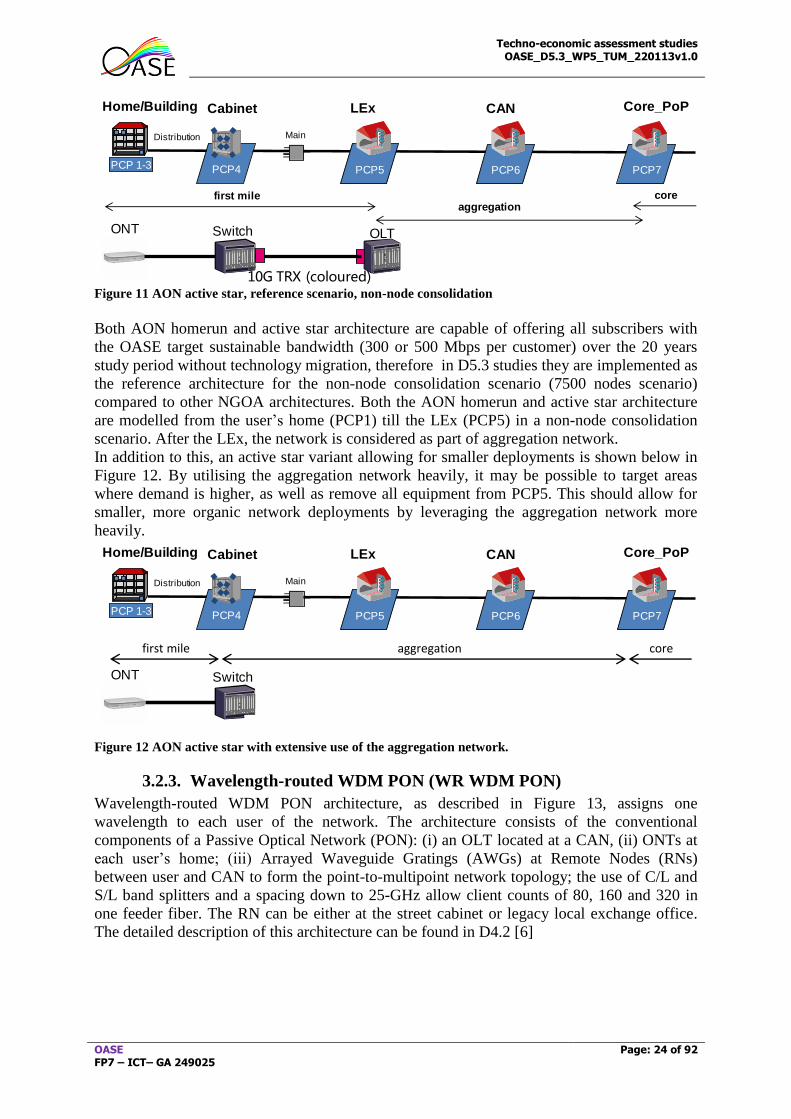
Unlike the homerun architecture, an active star architecture employs active remote node
(ARN) topology, as illustrated in Figure 11. The active equipment (in this case Ethernet
switches) are located in either cabinet or building locations where upstream data from a group
of end-users is aggregated, then the uplink of these Ethernet switches are further aggregated
into either a single or a few feeder fibres towards the second Ethernet switch at LEx (PCP5)
or CAN (PCP6).
1:32
first mile core
1 2
3
PCP4 PCP5 PCP6 PCP7
Distribution Main
PCP 1-3
Home/Building Cabinet LEx CAN Core_PoP
aggregation
SFP (grey, single-fiber)SFP (grey, single-fiber)
ONTOLT
Techno-economic assessment studies OASE_D5.3_WP5_TUM_220113v1.0
OASE FP7 – ICT– GA 249025
Page: 24 of 92
Figure 11 AON active star, reference scenario, non-node consolidation
Both AON homerun and active star architecture are capable of offering all subscribers with
the OASE target sustainable bandwidth (300 or 500 Mbps per customer) over the 20 years
study period without technology migration, therefore in D5.3 studies they are implemented as
the reference architecture for the non-node consolidation scenario (7500 nodes scenario)
compared to other NGOA architectures. Both the AON homerun and active star architecture
are modelled from the user’s home (PCP1) till the LEx (PCP5) in a non-node consolidation
scenario. After the LEx, the network is considered as part of aggregation network.
In addition to this, an active star variant allowing for smaller deployments is shown below in
Figure 12. By utilising the aggregation network heavily, it may be possible to target areas
where demand is higher, as well as remove all equipment from PCP5. This should allow for
smaller, more organic network deployments by leveraging the aggregation network more
heavily.
Figure 12 AON active star with extensive use of the aggregation network.
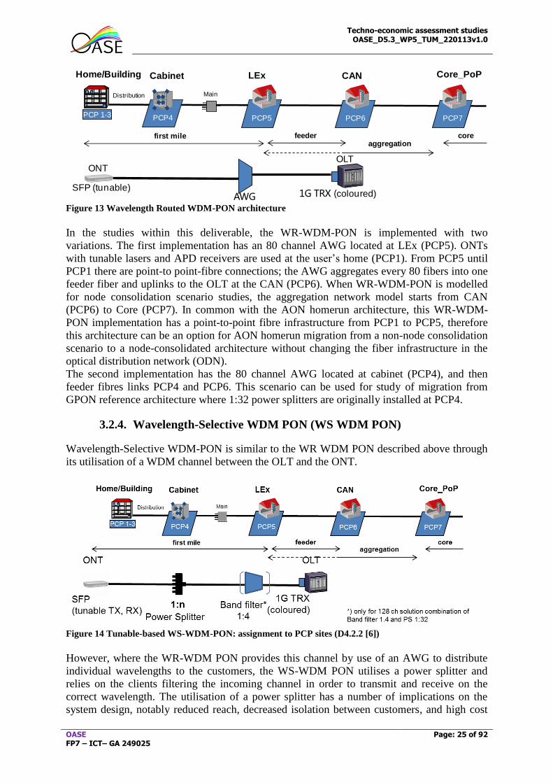
3.2.3. Wavelength-routed WDM PON (WR WDM PON)
Wavelength-routed WDM PON architecture, as described in Figure 13, assigns one
wavelength to each user of the network. The architecture consists of the conventional
components of a Passive Optical Network (PON): (i) an OLT located at a CAN, (ii) ONTs at
each user’s home; (iii) Arrayed Waveguide Gratings (AWGs) at Remote Nodes (RNs)
between user and CAN to form the point-to-multipoint network topology; the use of C/L and
S/L band splitters and a spacing down to 25-GHz allow client counts of 80, 160 and 320 in
one feeder fiber. The RN can be either at the street cabinet or legacy local exchange office.
The detailed description of this architecture can be found in D4.2 [6]
first mile core
1 2
3
PCP4 PCP5 PCP6 PCP7
Distribution Main
PCP 1-3
Home/Building Cabinet LEx CAN Core_PoP
aggregation
ONT Switch OLT
10G TRX (coloured)
first mile core
1 2
3
PCP4 PCP5 PCP6 PCP7
Distribution Main
PCP 1-3
Home/Building Cabinet LEx CAN Core_PoP
aggregation
ONT Switch OLT
10G TRX (coloured)
core first mile
aggregation
Techno-economic assessment studies OASE_D5.3_WP5_TUM_220113v1.0
OASE FP7 – ICT– GA 249025
Page: 25 of 92
Figure 13 Wavelength Routed WDM-PON architecture
In the studies within this deliverable, the WR-WDM-PON is implemented with two
variations. The first implementation has an 80 channel AWG located at LEx (PCP5). ONTs
with tunable lasers and APD receivers are used at the user’s home (PCP1). From PCP5 until
PCP1 there are point-to point-fibre connections; the AWG aggregates every 80 fibers into one
feeder fiber and uplinks to the OLT at the CAN (PCP6). When WR-WDM-PON is modelled
for node consolidation scenario studies, the aggregation network model starts from CAN
(PCP6) to Core (PCP7). In common with the AON homerun architecture, this WR-WDM-
PON implementation has a point-to-point fibre infrastructure from PCP1 to PCP5, therefore
this architecture can be an option for AON homerun migration from a non-node consolidation
scenario to a node-consolidated architecture without changing the fiber infrastructure in the
optical distribution network (ODN).
The second implementation has the 80 channel AWG located at cabinet (PCP4), and then
feeder fibres links PCP4 and PCP6. This scenario can be used for study of migration from
GPON reference architecture where 1:32 power splitters are originally installed at PCP4.
3.2.4. Wavelength-Selective WDM PON (WS WDM PON)
Wavelength-Selective WDM-PON is similar to the WR WDM PON described above through
its utilisation of a WDM channel between the OLT and the ONT.
Figure 14 Tunable-based WS-WDM-PON: assignment to PCP sites (D4.2.2 [6])
However, where the WR-WDM PON provides this channel by use of an AWG to distribute
individual wavelengths to the customers, the WS-WDM PON utilises a power splitter and
relies on the clients filtering the incoming channel in order to transmit and receive on the
correct wavelength. The utilisation of a power splitter has a number of implications on the
system design, notably reduced reach, decreased isolation between customers, and high cost
1:32
AWG
first mile feeder core
1 2
3
PCP4 PCP5 PCP6 PCP7
Distribution Main
PCP 1-3
Home/Building Cabinet LEx CAN Core_PoP
aggregation
ONTOLT
1G TRX (coloured)SFP (tunable)
Techno-economic assessment studies OASE_D5.3_WP5_TUM_220113v1.0
OASE FP7 – ICT– GA 249025
Page: 26 of 92
through necessitating the usage of expensive tuneable filters. However, these issues are offset
by its inherent potential for simple migration from GPON by utilising the already-deployed
optical splitters in the passive infrastructure. One of the interesting assessments will be the
trade-off between higher system cost and cost savings through passive infrastructure re-use.
WS-WDM PON exists in three variants, based around the number of wavelengths per fibre.
The 32 channel system provides the best alignment with GPON optical splitter deployments,
while the 64 channel system offers the possibility of higher fan out with associated reach
penalty. Finally, a 128 wavelength system is available, utilising a DWDM band splitter
located in PCP5 to create 4 32 way splits. This offers the highest fan-out while still retaining
compatibility with the conventional GPON passive infrastructure, but requires the use of
EDFA boosters/pre-amplifiers co-located with the line cards with corresponding increase in
system cost.
Further information about this architecture variant may be found in D4.2 [6].
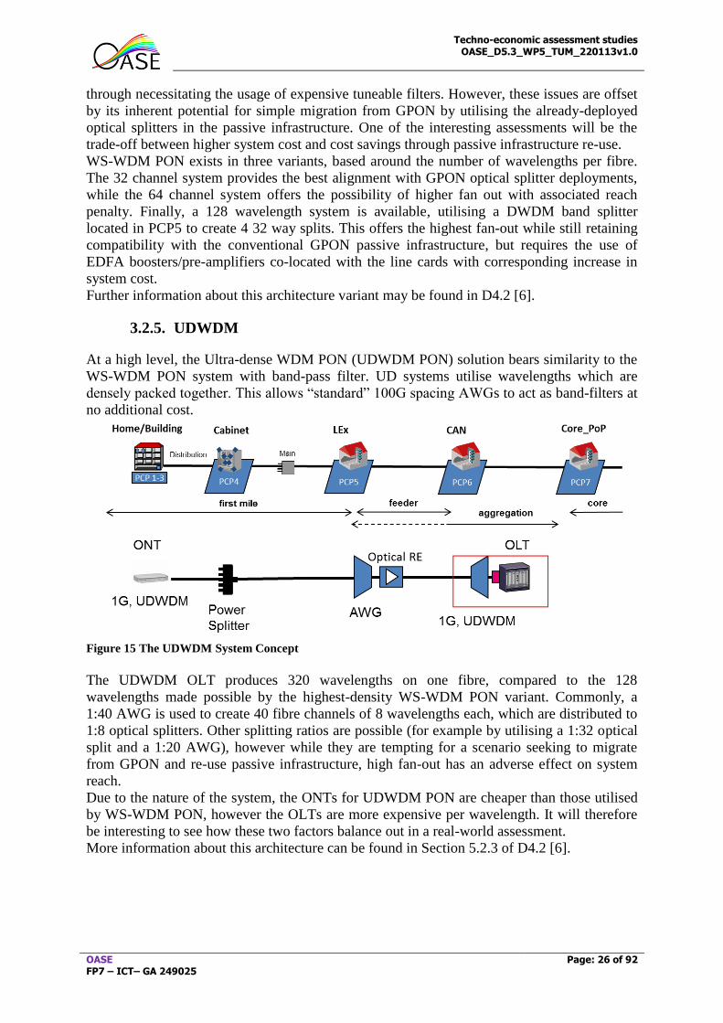
3.2.5. UDWDM
At a high level, the Ultra-dense WDM PON (UDWDM PON) solution bears similarity to the
WS-WDM PON system with band-pass filter. UD systems utilise wavelengths which are
densely packed together. This allows “standard” 100G spacing AWGs to act as band-filters at
no additional cost.
Figure 15 The UDWDM System Concept
The UDWDM OLT produces 320 wavelengths on one fibre, compared to the 128
wavelengths made possible by the highest-density WS-WDM PON variant. Commonly, a
1:40 AWG is used to create 40 fibre channels of 8 wavelengths each, which are distributed to
1:8 optical splitters. Other splitting ratios are possible (for example by utilising a 1:32 optical
split and a 1:20 AWG), however while they are tempting for a scenario seeking to migrate
from GPON and re-use passive infrastructure, high fan-out has an adverse effect on system
reach.
Due to the nature of the system, the ONTs for UDWDM PON are cheaper than those utilised
by WS-WDM PON, however the OLTs are more expensive per wavelength. It will therefore
be interesting to see how these two factors balance out in a real-world assessment.
More information about this architecture can be found in Section 5.2.3 of D4.2 [6].

Techno-economic assessment studies OASE_D5.3_WP5_TUM_220113v1.0
OASE FP7 – ICT– GA 249025
Page: 27 of 92
3.2.6. Passive Hybrid PON
The passive Hybrid PON (HPON) considered in these studies is shown in Figure 16. It
consists of two splitting points: the power splitter located at PCP4 and the wavelength splitter
(Array Waveguide: AWG) at PCP5. The OLT is located at PCP5 for the non-node
consolidation studies and at PCP6 for the consolidation studies. Two different splitting ratios
have been considered:
“HPON40”: considers an AWG with 40 channels, and a 1:32 power splitter. APD
receivers are considered at the ONT.
“HPON80” considers an AWG with 80 channels and a 1:16 power splitter. PIN
receivers are assumed to be used at the ONTs and hence, reach extenders may be
needed at PCP5.
Figure 16 HPON architecture in case of node consolidation
Both architectures have the same client count but HPON80 offers higher bandwidth than
HPON40.
3.2.7. WDM PON backhauling AON
A WDM PON backhauling solution can be adopted in order to migrate AON active star
architectures from a non-node consolidation scenario to a node consolidation scenario by
replacing the active equipment previously located at PCP5 with passive AWGs, meanwhile a
WDM OLT is placed at the CAN (PCP6), thus the access network is extended, and the
aggregation network starts from PCP6 to PCP7.
Figure 17 WDM PON backhauling AON
first mile feeder core
1 2
3
PCP4 PCP5 PCP6 PCP7
Distribution Main
PCP 1-3
Home/Building Cabinet LEx CAN Core_PoP
aggregation
ONT LEx SwitchOLT
10G TRX (coloured) AWG 10G TRX(coloured)AWG
Techno-economic assessment studies OASE_D5.3_WP5_TUM_220113v1.0
OASE FP7 – ICT– GA 249025
Page: 28 of 92
The migration from the reference AON active star outlined in the sections above to WDM
PON backhauling architecture can be done smoothly without changing the fibre infrastructure
in the ODN from PCP1 to PCP5, the ONTs at PCP1 and switches at PCP4 can be reused as
well.
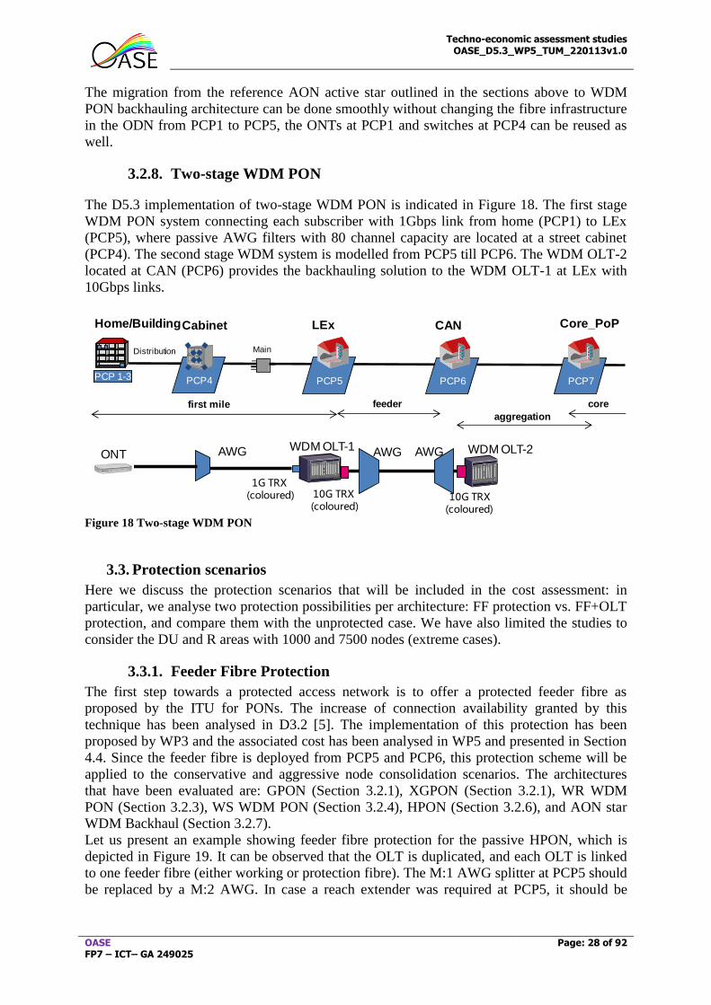
3.2.8. Two-stage WDM PON
The D5.3 implementation of two-stage WDM PON is indicated in Figure 18. The first stage
WDM PON system connecting each subscriber with 1Gbps link from home (PCP1) to LEx
(PCP5), where passive AWG filters with 80 channel capacity are located at a street cabinet
(PCP4). The second stage WDM system is modelled from PCP5 till PCP6. The WDM OLT-2
located at CAN (PCP6) provides the backhauling solution to the WDM OLT-1 at LEx with
10Gbps links.
Figure 18 Two-stage WDM PON
3.3. Protection scenarios
Here we discuss the protection scenarios that will be included in the cost assessment: in
particular, we analyse two protection possibilities per architecture: FF protection vs. FF+OLT
protection, and compare them with the unprotected case. We have also limited the studies to
consider the DU and R areas with 1000 and 7500 nodes (extreme cases).
3.3.1. Feeder Fibre Protection
The first step towards a protected access network is to offer a protected feeder fibre as
proposed by the ITU for PONs. The increase of connection availability granted by this
technique has been analysed in D3.2 [5]. The implementation of this protection has been
proposed by WP3 and the associated cost has been analysed in WP5 and presented in Section
4.4. Since the feeder fibre is deployed from PCP5 and PCP6, this protection scheme will be
applied to the conservative and aggressive node consolidation scenarios. The architectures
that have been evaluated are: GPON (Section 3.2.1), XGPON (Section 3.2.1), WR WDM
PON (Section 3.2.3), WS WDM PON (Section 3.2.4), HPON (Section 3.2.6), and AON star
WDM Backhaul (Section 3.2.7).
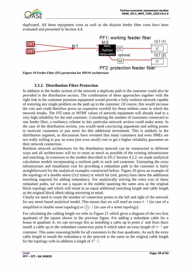
Let us present an example showing feeder fibre protection for the passive HPON, which is
depicted in Figure 19. It can be observed that the OLT is duplicated, and each OLT is linked
to one feeder fibre (either working or protection fibre). The M:1 AWG splitter at PCP5 should
be replaced by a M:2 AWG. In case a reach extender was required at PCP5, it should be
first mile feeder core
1 2
3
PCP4 PCP5 PCP6 PCP7
Distribution Main
PCP 1-3
Home/BuildingCabinet LEx CAN Core_PoP
aggregation
ONTWDM OLT-1 WDM OLT-2
10G TRX(coloured)
AWG
10G TRX (coloured)
AWGAWG
1G TRX(coloured)
Techno-economic assessment studies OASE_D5.3_WP5_TUM_220113v1.0
OASE FP7 – ICT– GA 249025
Page: 29 of 92
duplicated. All these equipment costs as well as the disjoint feeder fibre costs have been
evaluated and presented in Section 4.4.
Figure 19 Feeder Fiber (FF) protection for HPON architecture
3.3.2. Distribution Fibre Protection
In addition to the feeder section of the network a duplicate path to the customer could also be
provided in the distribution section. The combination of these approaches together with the
right link in the customer premises equipment would provide a fully resilient network capable
of restoring any single problem on the path up to the customer. Of course, this would increase
the cost and could therefore prove an expensive overkill for those seldom cases in which the
network breaks. The FIT-rates or MTBF values of network equipment will already lead to a
very high reliability for the end customer. Considering the number of customers connected to
one feeder fibre, a resiliency scheme in this particular network section could make sense. In
the case of the distribution section, you would need convincing arguments and selling points
to motivate customers to pay more for this additional investment. This is unlikely in the
distribution segment, as discussions have revealed that many customers and even SMEs are
not really willing to pay an extra (not even small) cost to get a higher reliability guarantee on
their network connection.
Resilient network architectures for the distribution network can be constructed in different
ways and all architectures will try to reuse as much as possible of the existing infrastructure
and trenching. In extension to the models described in D5.2 Section 4.2.2, we made analytical
calculation models incorporating a resilient path to each end customer. Estimating the extra
infrastructure and installation cost for providing a redundant path to the customer is fairly
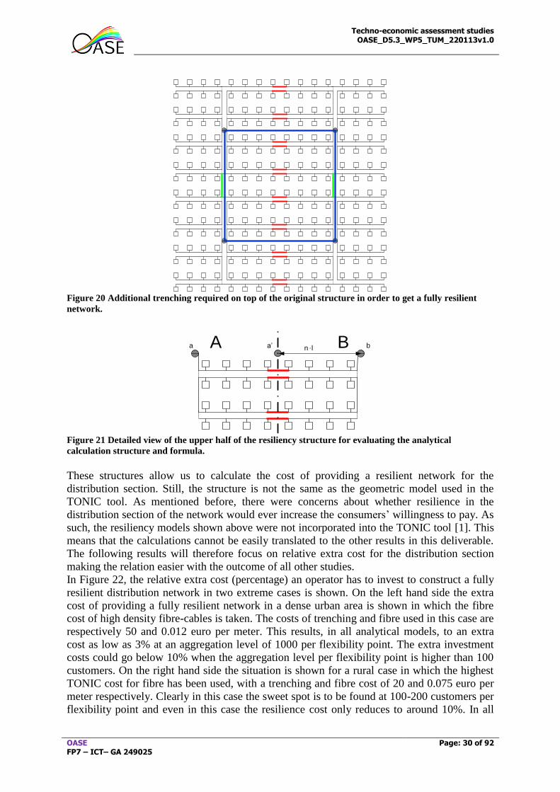
straightforward for the analytical examples constructed before. Figure 20 gives an example of
the topology of a double street (2x2 times) in which fat (red, green) lines show the additional
trenching required for adding redundancy. For analytically solving the extra cost of these
redundant paths, we cut out a square in the middle spanning the same area as the original
block topology and which will result in an equal additional trenching length and cable length
as the original block albeit taking mirroring in mind.
Clearly we need to count the number of connection points to the left and right of the network
for any street based analytical model. This means that we will need an extra (in case of a
simplified or double street topology) or (in case of a street topology).
For calculating the cabling length we refer to Figure 21 which gives a diagram of the two first
quadrants of the square shown in the previous figure. For adding a redundant cable for a
house in quadrant A, we can envisage this as installing a cable up to point a’ and from there
install a cable up to the redundant connection point b which takes an extra length of per
customer. This same reasoning holds for all customers in the four quadrants. As such the extra
cable length to install the redundancy in the network is the same as the original cable length
for the topology with in addition a length of .
Techno-economic assessment studies OASE_D5.3_WP5_TUM_220113v1.0
OASE FP7 – ICT– GA 249025
Page: 30 of 92
Figure 20 Additional trenching required on top of the original structure in order to get a fully resilient
network.
Figure 21 Detailed view of the upper half of the resiliency structure for evaluating the analytical
calculation structure and formula.
These structures allow us to calculate the cost of providing a resilient network for the
distribution section. Still, the structure is not the same as the geometric model used in the
TONIC tool. As mentioned before, there were concerns about whether resilience in the
distribution section of the network would ever increase the consumers’ willingness to pay. As
such, the resiliency models shown above were not incorporated into the TONIC tool [1]. This
means that the calculations cannot be easily translated to the other results in this deliverable.
The following results will therefore focus on relative extra cost for the distribution section
making the relation easier with the outcome of all other studies.
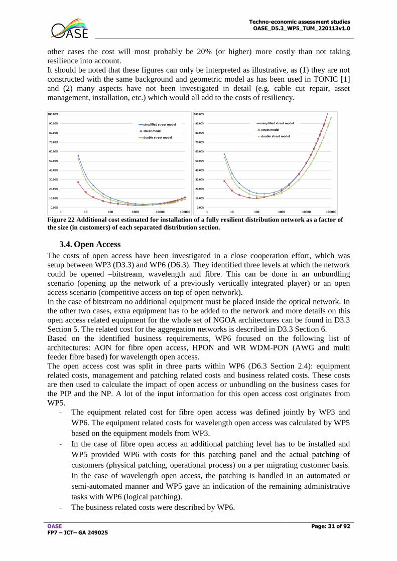
In Figure 22, the relative extra cost (percentage) an operator has to invest to construct a fully
resilient distribution network in two extreme cases is shown. On the left hand side the extra
cost of providing a fully resilient network in a dense urban area is shown in which the fibre
cost of high density fibre-cables is taken. The costs of trenching and fibre used in this case are
respectively 50 and 0.012 euro per meter. This results, in all analytical models, to an extra
cost as low as 3% at an aggregation level of 1000 per flexibility point. The extra investment
costs could go below 10% when the aggregation level per flexibility point is higher than 100
customers. On the right hand side the situation is shown for a rural case in which the highest
TONIC cost for fibre has been used, with a trenching and fibre cost of 20 and 0.075 euro per
meter respectively. Clearly in this case the sweet spot is to be found at 100-200 customers per
flexibility point and even in this case the resilience cost only reduces to around 10%. In all
A Ba ba’ n l.
Techno-economic assessment studies OASE_D5.3_WP5_TUM_220113v1.0
OASE FP7 – ICT– GA 249025
Page: 31 of 92
other cases the cost will most probably be 20% (or higher) more costly than not taking
resilience into account.
It should be noted that these figures can only be interpreted as illustrative, as (1) they are not
constructed with the same background and geometric model as has been used in TONIC [1]
and (2) many aspects have not been investigated in detail (e.g. cable cut repair, asset
management, installation, etc.) which would all add to the costs of resiliency.
Figure 22 Additional cost estimated for installation of a fully resilient distribution network as a factor of
the size (in customers) of each separated distribution section.
3.4. Open Access
The costs of open access have been investigated in a close cooperation effort, which was
setup between WP3 (D3.3) and WP6 (D6.3). They identified three levels at which the network
could be opened –bitstream, wavelength and fibre. This can be done in an unbundling
scenario (opening up the network of a previously vertically integrated player) or an open
access scenario (competitive access on top of open network).
In the case of bitstream no additional equipment must be placed inside the optical network. In
the other two cases, extra equipment has to be added to the network and more details on this
open access related equipment for the whole set of NGOA architectures can be found in D3.3
Section 5. The related cost for the aggregation networks is described in D3.3 Section 6.
Based on the identified business requirements, WP6 focused on the following list of
architectures: AON for fibre open access, HPON and WR WDM-PON (AWG and multi
feeder fibre based) for wavelength open access.
The open access cost was split in three parts within WP6 (D6.3 Section 2.4): equipment
related costs, management and patching related costs and business related costs. These costs
are then used to calculate the impact of open access or unbundling on the business cases for
the PIP and the NP. A lot of the input information for this open access cost originates from
WP5.
- The equipment related cost for fibre open access was defined jointly by WP3 and
WP6. The equipment related costs for wavelength open access was calculated by WP5
based on the equipment models from WP3.
- In the case of fibre open access an additional patching level has to be installed and
WP5 provided WP6 with costs for this patching panel and the actual patching of
customers (physical patching, operational process) on a per migrating customer basis.
In the case of wavelength open access, the patching is handled in an automated or
semi-automated manner and WP5 gave an indication of the remaining administrative
tasks with WP6 (logical patching).
- The business related costs were described by WP6.
0.00%
10.00%
20.00%
30.00%
40.00%
50.00%
60.00%
70.00%
80.00%
90.00%
100.00%
1 10 100 1000 10000 100000
simplified street model
street model
double street model
0.00%
10.00%
20.00%
30.00%
40.00%
50.00%
60.00%
70.00%
80.00%
90.00%
100.00%
1 10 100 1000 10000 100000
simplified street model
street model
double street model
Techno-economic assessment studies OASE_D5.3_WP5_TUM_220113v1.0
OASE FP7 – ICT– GA 249025
Page: 32 of 92
As mentioned for all details on the architectures we refer to D3.3 and for further analysis of
the impact on the costs of introducing open access, we refer to D6.3.
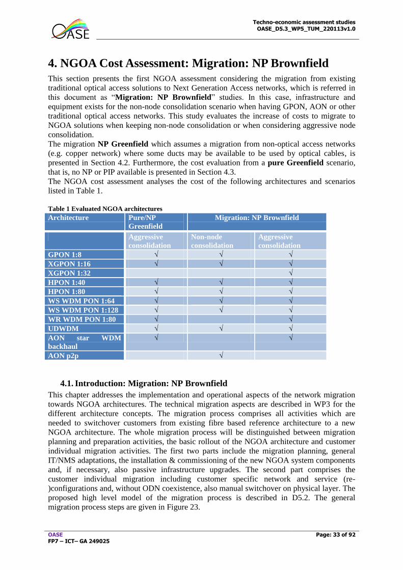
Techno-economic assessment studies OASE_D5.3_WP5_TUM_220113v1.0
OASE FP7 – ICT– GA 249025
Page: 33 of 92
4. NGOA Cost Assessment: Migration: NP Brownfield
This section presents the first NGOA assessment considering the migration from existing
traditional optical access solutions to Next Generation Access networks, which is referred in
this document as “Migration: NP Brownfield” studies. In this case, infrastructure and
equipment exists for the non-node consolidation scenario when having GPON, AON or other
traditional optical access networks. This study evaluates the increase of costs to migrate to
NGOA solutions when keeping non-node consolidation or when considering aggressive node
consolidation.
The migration NP Greenfield which assumes a migration from non-optical access networks
(e.g. copper network) where some ducts may be available to be used by optical cables, is
presented in Section 4.2. Furthermore, the cost evaluation from a pure Greenfield scenario,
that is, no NP or PIP available is presented in Section 4.3.
The NGOA cost assessment analyses the cost of the following architectures and scenarios
listed in Table 1.
Table 1 Evaluated NGOA architectures
Architecture Pure/NP
Greenfield
Migration: NP Brownfield
Aggressive
consolidation
Non-node
consolidation
Aggressive
consolidation
GPON 1:8 √ √ √
XGPON 1:16 √ √ √
XGPON 1:32 √
HPON 1:40 √ √ √
HPON 1:80 √ √ √
WS WDM PON 1:64 √ √ √
WS WDM PON 1:128 √ √ √
WR WDM PON 1:80 √ √
UDWDM √ √ √
AON star WDM
backhaul
√ √
AON p2p √
4.1. Introduction: Migration: NP Brownfield
This chapter addresses the implementation and operational aspects of the network migration
towards NGOA architectures. The technical migration aspects are described in WP3 for the
different architecture concepts. The migration process comprises all activities which are
needed to switchover customers from existing fibre based reference architecture to a new
NGOA architecture. The whole migration process will be distinguished between migration
planning and preparation activities, the basic rollout of the NGOA architecture and customer
individual migration activities. The first two parts include the migration planning, general
IT/NMS adaptations, the installation & commissioning of the new NGOA system components
and, if necessary, also passive infrastructure upgrades. The second part comprises the
customer individual migration including customer specific network and service (re-
)configurations and, without ODN coexistence, also manual switchover on physical layer. The
proposed high level model of the migration process is described in D5.2. The general
migration process steps are given in Figure 23.
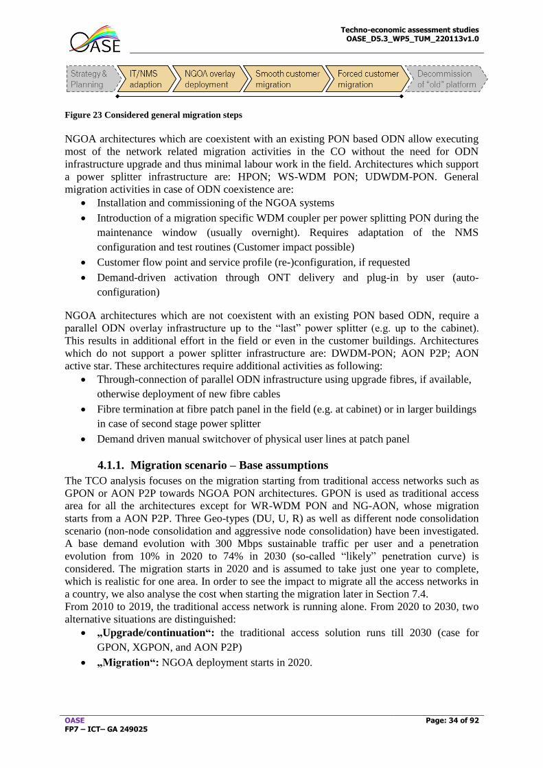
Techno-economic assessment studies OASE_D5.3_WP5_TUM_220113v1.0
OASE FP7 – ICT– GA 249025
Page: 34 of 92
Figure 23 Considered general migration steps
NGOA architectures which are coexistent with an existing PON based ODN allow executing
most of the network related migration activities in the CO without the need for ODN
infrastructure upgrade and thus minimal labour work in the field. Architectures which support
a power splitter infrastructure are: HPON; WS-WDM PON; UDWDM-PON. General
migration activities in case of ODN coexistence are:
Installation and commissioning of the NGOA systems
Introduction of a migration specific WDM coupler per power splitting PON during the
maintenance window (usually overnight). Requires adaptation of the NMS
configuration and test routines (Customer impact possible)
Customer flow point and service profile (re-)configuration, if requested
Demand-driven activation through ONT delivery and plug-in by user (auto-
configuration)
NGOA architectures which are not coexistent with an existing PON based ODN, require a
parallel ODN overlay infrastructure up to the “last” power splitter (e.g. up to the cabinet).
This results in additional effort in the field or even in the customer buildings. Architectures
which do not support a power splitter infrastructure are: DWDM-PON; AON P2P; AON
active star. These architectures require additional activities as following:
Through-connection of parallel ODN infrastructure using upgrade fibres, if available,
otherwise deployment of new fibre cables
Fibre termination at fibre patch panel in the field (e.g. at cabinet) or in larger buildings
in case of second stage power splitter
Demand driven manual switchover of physical user lines at patch panel
4.1.1. Migration scenario – Base assumptions
The TCO analysis focuses on the migration starting from traditional access networks such as
GPON or AON P2P towards NGOA PON architectures. GPON is used as traditional access
area for all the architectures except for WR-WDM PON and NG-AON, whose migration
starts from a AON P2P. Three Geo-types (DU, U, R) as well as different node consolidation
scenario (non-node consolidation and aggressive node consolidation) have been investigated.
A base demand evolution with 300 Mbps sustainable traffic per user and a penetration
evolution from 10% in 2020 to 74% in 2030 (so-called “likely” penetration curve) is
considered. The migration starts in 2020 and is assumed to take just one year to complete,
which is realistic for one area. In order to see the impact to migrate all the access networks in
a country, we also analyse the cost when starting the migration later in Section 7.4.
From 2010 to 2019, the traditional access network is running alone. From 2020 to 2030, two
alternative situations are distinguished:
„Upgrade/continuation“: the traditional access solution runs till 2030 (case for
GPON, XGPON, and AON P2P)
„Migration“: NGOA deployment starts in 2020.
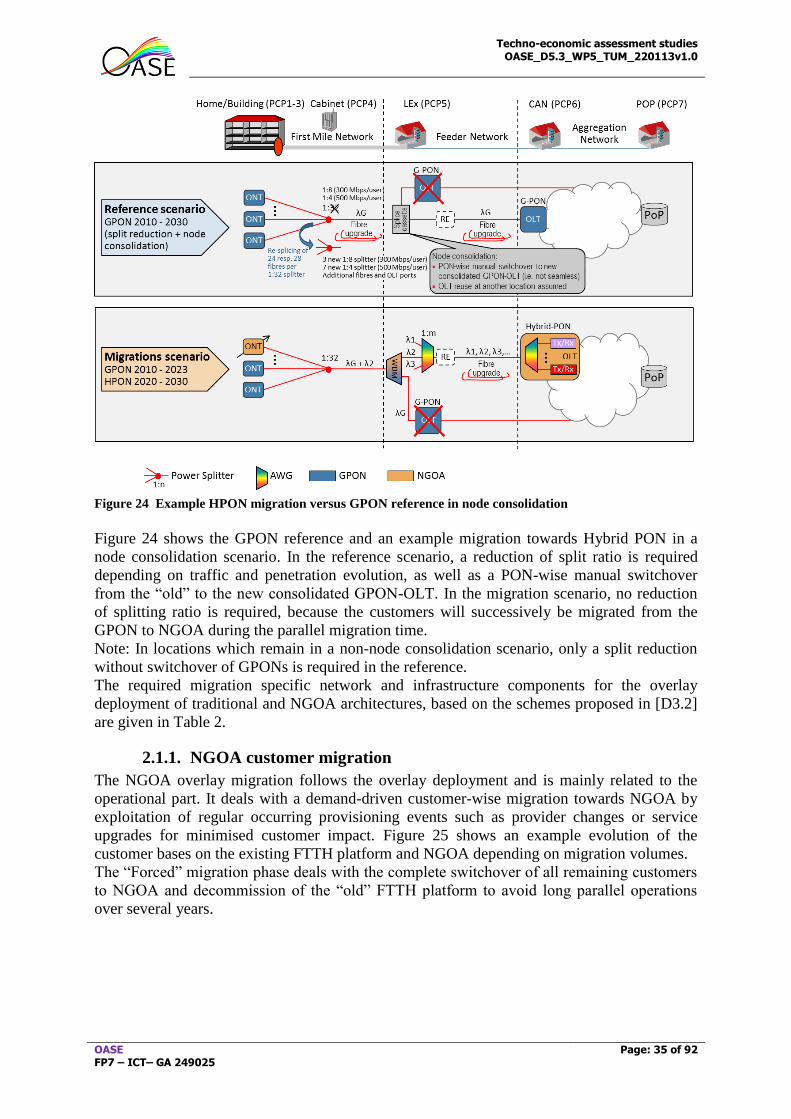
Techno-economic assessment studies OASE_D5.3_WP5_TUM_220113v1.0
OASE FP7 – ICT– GA 249025
Page: 35 of 92
Figure 24 Example HPON migration versus GPON reference in node consolidation
Figure 24 shows the GPON reference and an example migration towards Hybrid PON in a
node consolidation scenario. In the reference scenario, a reduction of split ratio is required
depending on traffic and penetration evolution, as well as a PON-wise manual switchover
from the “old” to the new consolidated GPON-OLT. In the migration scenario, no reduction
of splitting ratio is required, because the customers will successively be migrated from the
GPON to NGOA during the parallel migration time.
Note: In locations which remain in a non-node consolidation scenario, only a split reduction
without switchover of GPONs is required in the reference.
The required migration specific network and infrastructure components for the overlay
deployment of traditional and NGOA architectures, based on the schemes proposed in [D3.2]
are given in Table 2.
2.1.1. NGOA customer migration
The NGOA overlay migration follows the overlay deployment and is mainly related to the
operational part. It deals with a demand-driven customer-wise migration towards NGOA by
exploitation of regular occurring provisioning events such as provider changes or service
upgrades for minimised customer impact. Figure 25 shows an example evolution of the
customer bases on the existing FTTH platform and NGOA depending on migration volumes.
The “Forced” migration phase deals with the complete switchover of all remaining customers
to NGOA and decommission of the “old” FTTH platform to avoid long parallel operations
over several years.
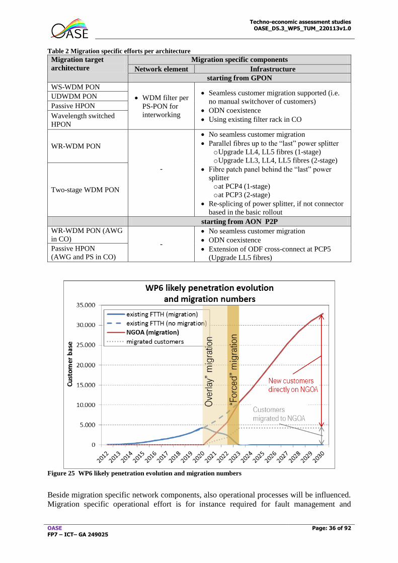
Techno-economic assessment studies OASE_D5.3_WP5_TUM_220113v1.0
OASE FP7 – ICT– GA 249025
Page: 36 of 92
Table 2 Migration specific efforts per architecture
Migration target
architecture
Migration specific components
Network element Infrastructure
starting from GPON
WS-WDM PON
WDM filter per
PS-PON for
interworking
Seamless customer migration supported (i.e.
no manual switchover of customers)
ODN coexistence
Using existing filter rack in CO
UDWDM PON
Passive HPON
Wavelength switched
HPON
WR-WDM PON
-
No seamless customer migration
Parallel fibres up to the “last” power splitter
o Upgrade LL4, LL5 fibres (1-stage)
o Upgrade LL3, LL4, LL5 fibres (2-stage)
Fibre patch panel behind the “last” power
splitter
o at PCP4 (1-stage)
o at PCP3 (2-stage)
Re-splicing of power splitter, if not connector
based in the basic rollout
Two-stage WDM PON
starting from AON P2P
WR-WDM PON (AWG
in CO) -
No seamless customer migration
ODN coexistence
Extension of ODF cross-connect at PCP5
(Upgrade LL5 fibres) Passive HPON
(AWG and PS in CO)
Figure 25 WP6 likely penetration evolution and migration numbers
Beside migration specific network components, also operational processes will be influenced.
Migration specific operational effort is for instance required for fault management and
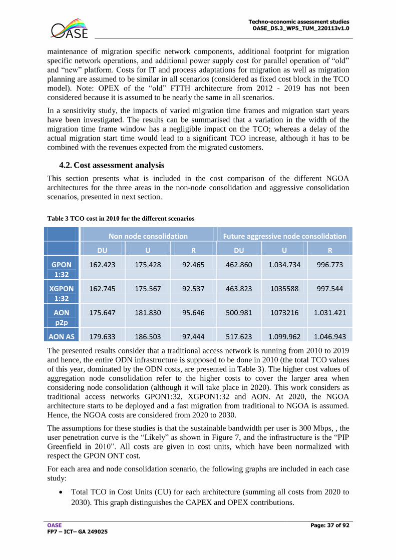
Techno-economic assessment studies OASE_D5.3_WP5_TUM_220113v1.0
OASE FP7 – ICT– GA 249025
Page: 37 of 92
maintenance of migration specific network components, additional footprint for migration
specific network operations, and additional power supply cost for parallel operation of “old”
and “new” platform. Costs for IT and process adaptations for migration as well as migration
planning are assumed to be similar in all scenarios (considered as fixed cost block in the TCO
model). Note: OPEX of the “old” FTTH architecture from 2012 - 2019 has not been
considered because it is assumed to be nearly the same in all scenarios.
In a sensitivity study, the impacts of varied migration time frames and migration start years
have been investigated. The results can be summarised that a variation in the width of the
migration time frame window has a negligible impact on the TCO; whereas a delay of the
actual migration start time would lead to a significant TCO increase, although it has to be
combined with the revenues expected from the migrated customers.
4.2. Cost assessment analysis
This section presents what is included in the cost comparison of the different NGOA
architectures for the three areas in the non-node consolidation and aggressive consolidation
scenarios, presented in next section.
Table 3 TCO cost in 2010 for the different scenarios
The presented results consider that a traditional access network is running from 2010 to 2019
and hence, the entire ODN infrastructure is supposed to be done in 2010 (the total TCO values
of this year, dominated by the ODN costs, are presented in Table 3). The higher cost values of
aggregation node consolidation refer to the higher costs to cover the larger area when
considering node consolidation (although it will take place in 2020). This work considers as
traditional access networks GPON1:32, XGPON1:32 and AON. At 2020, the NGOA
architecture starts to be deployed and a fast migration from traditional to NGOA is assumed.
Hence, the NGOA costs are considered from 2020 to 2030.
The assumptions for these studies is that the sustainable bandwidth per user is 300 Mbps, , the
user penetration curve is the “Likely” as shown in Figure 7, and the infrastructure is the “PIP
Greenfield in 2010”. All costs are given in cost units, which have been normalized with
respect the GPON ONT cost.
For each area and node consolidation scenario, the following graphs are included in each case
study:
Total TCO in Cost Units (CU) for each architecture (summing all costs from 2020 to
2030). This graph distinguishes the CAPEX and OPEX contributions.
Non node consolidation Future aggressive node consolidation
DU U R DU U R
GPON 1:32
162.423 175.428 92.465 462.860 1.034.734 996.773
XGPON 1:32
162.745 175.567 92.537 463.823 1035588 997.544
AON p2p
175.647 181.830 95.646 500.981 1073216 1.031.421
AON AS 179.633 186.503 97.444 517.623 1.099.962 1.046.943
Techno-economic assessment studies OASE_D5.3_WP5_TUM_220113v1.0
OASE FP7 – ICT– GA 249025
Page: 38 of 92
Total CAPEX in cost units [CU] and CAPEX per users connected in 2030 [CU/user]
gives for each architecture the sum of the non-discounted CAPEX which include:
o PIP Infrastructure (PIP Infra) such as distribution fibre, distribution duct,
installation costs, cabinet, etc.
o PIP Equipment (PIP Equip) such as power splitters, wavelength splitters, etc.
o In house infrastructure (In house Infra) such as in house cabling and its
installation costs
o CPE Equipment (CPE Equip) includes the ONT cost as well as its installation
cost
o Network Provider costs (NP) includes OLT and any active equipment in the
field such as reach extenders, Ethernet switches, etc.
Total OPEX in cost units [CU] and OPEX per user [CU/user] gives for each
architecture the sum of the non-discounted OPEX which include:
o Fault Management (FM) which is the fault management costs associated to the
failures in any equipment and infrastructure expect the CPE.
o Fault Management of the CPE (CPE FM)
o Energy gives the energy cost of the power consumed by any equipment except
the CPE
o CPE Energy is the energy cost of the power consumed by the CPE
o Service Provisioning (SP) is the cost associated to any physical installation,
service connection and service disconnection required by the users.
o Floor space includes the cost of the floor space required by the OLT at the
operator premises as well as any active component required in the field.
Non-discounted TCO [CU] gives the non-discounted TCO per year excluding the
2010 as previously mentioned.
Discounted TCO [CU] gives for comparative reasons, the discounted TCO per year. In
this study, 5% and 10% discount rates [7] have been considered for physical
infrastructure and equipment respectively.
Finally, the average TCO per connected user per year shows the average over the
years 2020-2030 of the TCO per users, taking into account the users which are
connected in each year (based on the penetration curve).
All graphs on the CAPEX and OPEX show the costs in a non-discounted manner. In this way,
the real cost is shown as experienced in the given years. While this gives a very good view on
when to expect which costs in both investments (CAPEX) as well as operations (OPEX), it
gives no information on the relation between both in terms of a business case. Typically the
weight of an investment on a business case will diminish with a later investment time due to
the effect this cost has on the risk of the business case. A company would want a return at
least equal to its Weighted Average Cost of Capital (WACC), which represents the percentage
costs a company incurs for lending or freeing this amount of money. This has been taken into
account in the discounted TCO.
For each scenario covered in Sections 4.3 and 4.4, a graph showing the average non
discounted TCO per connected user per year is also given. In this case it reflects the
undiscounted cost spread over all subscription years and this can be interpreted as the fee that
a customer should be paying in order to have a break-even for the network infrastructure. A
note of warning should be given with this though. The costs of the network represent actually
Techno-economic assessment studies OASE_D5.3_WP5_TUM_220113v1.0
OASE FP7 – ICT– GA 249025
Page: 39 of 92
only the costs for deploying an FTTH network up to the customer and providing the customer
with a CPE to connect on this network. It does not take into account the additional costs
required for providing services such as IPTV over this network, not from software and
management point of view, nor from content point of view. It does also not take into account
any costs for selling the services to the customer and marketing the network services. Taking
both these notes into account, it could still prove very meaningful for an operator to get an
idea of the cost-portion to spend per subscription for the network side. Operators will have a
means of comparing to more detailed cost figures enabling them to find out whether
deploying and maintaining such NGOA network could be more profitable than the current
network infrastructure.
Still one additional note of advice will be required. The current presentation of the costs on a
per subscription base are calculated without taking discounting into account. As most of the
costs are probably incurred during the first year, this will be almost the same as the discounted
costs per subscription. Taking discounting into account, this does not directly translate into
the subscription rate, as this subscription rate should be taking the same discounting into
account as well. In order to get a view on the subscription price to charge in order to get a
positive NPV, the following formula should be used:
With NPV = total calculated NPV
years = 0 .. planning horizon (here 0-20)
i = discount rate (often the same as WACC)
CF = cash flow for a given year
We want to know how much a customer subscription should generate to get break even
(considering the given discount rate of course). This means that we should change NPV by
the NPV per subscription year. We should cover the costs which are now the only component
in the cash flows by constant revenue flows (CRF) per customer subscription year (CRF
later). This makes the formula into the formula below:
The first term comes as a result from TONIC and we are interested in the value of CRF in the
first term. We will work with this in the further analysis:
This last term can be reduced analytically (is the sum of a geometric series) into
In which a = 1, r = (1+i)-1
and the years are running from 0 till 19 (inclusive)
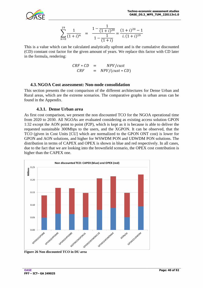
Techno-economic assessment studies OASE_D5.3_WP5_TUM_220113v1.0
OASE FP7 – ICT– GA 249025
Page: 40 of 92
This is a value which can be calculated analytically upfront and is the cumulative discounted
(CD) constant cost factor for the given amount of years. We replace this factor with CD later
in the formula, rendering:
4.3. NGOA Cost assessment: Non-node consolidation
This section presents the cost comparison of the different architectures for Dense Urban and
Rural areas, which are the extreme scenarios. The comparative graphs in urban areas can be
found in the Appendix.
4.3.1. Dense Urban area
As first cost comparison, we present the non discounted TCO for the NGOA operational time
from 2020 to 2030. All NGOAs are evaluated considering as existing access solution GPON
1:32 except the AON point to point (P2P), which is kept as it is because is able to deliver the
requested sustainable 300Mbps to the users, and the XGPON. It can be observed, that the
TCO (given in Cost Units [CU] which are normalized to the GPON ONT cost) is lower for
GPON and AON solutions, and higher for WSWDM PON and UDWDM PON solutions. The
distribution in terms of CAPEX and OPEX is shown in blue and red respectively. In all cases,
due to the fact that we are looking into the brownfield scenario, the OPEX cost contribution is
higher than the CAPEX one.
Figure 26 Non discounted TCO in DU area
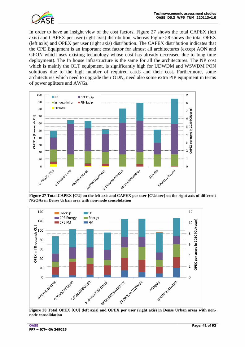
Techno-economic assessment studies OASE_D5.3_WP5_TUM_220113v1.0
OASE FP7 – ICT– GA 249025
Page: 41 of 92
In order to have an insight view of the cost factors, Figure 27 shows the total CAPEX (left
axis) and CAPEX per user (right axis) distribution, whereas Figure 28 shows the total OPEX
(left axis) and OPEX per user (right axis) distribution. The CAPEX distribution indicates that
the CPE Equipment is an important cost factor for almost all architectures (except AON and
GPON which uses existing technology whose cost has already decreased due to long time
deployment). The In house infrastructure is the same for all the architectures. The NP cost
which is mainly the OLT equipment, is significantly high for UDWDM and WSWDM PON
solutions due to the high number of required cards and their cost. Furthermore, some
architectures which need to upgrade their ODN, need also some extra PIP equipment in terms
of power splitters and AWGs.
Figure 27 Total CAPEX [CU] on the left axis and CAPEX per user [CU/user] on the right axis of different
NGOAs in Dense Urban area with non-node consolidation
Figure 28 Total OPEX [CU] (left axis) and OPEX per user (right axis) in Dense Urban areas with non-
node consolidation
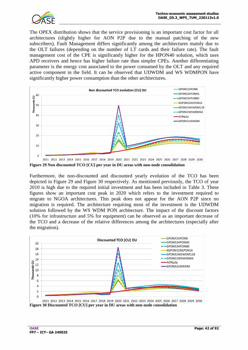
Techno-economic assessment studies OASE_D5.3_WP5_TUM_220113v1.0
OASE FP7 – ICT– GA 249025
Page: 42 of 92
The OPEX distribution shows that the service provisioning is an important cost factor for all
architectures (slightly higher for AON P2P due to the manual patching of the new
subscribers). Fault Management differs significantly among the architectures mainly due to
the OLT failures (depending on the number of LT cards and their failure rate). The fault
management cost of the CPE is significantly higher for the HPON40 solution, which uses
APD receivers and hence has higher failure rate than simpler CPEs. Another differentiating
parameter is the energy cost associated to the power consumed by the OLT and any required
active component in the field. It can be observed that UDWDM and WS WDMPON have
significantly higher power consumption than the other architectures.
Figure 29 Non discounted TCO [CU] per year in DU areas with non-node consolidation
Furthermore, the non-discounted and discounted yearly evolution of the TCO has been
depicted in Figure 29 and Figure 30 respectively. As mentioned previously, the TCO of year
2010 is high due to the required initial investment and has been included in Table 3. These
figures show an important cost peak in 2020 which refers to the investment required to
migrate to NGOA architectures. This peak does not appear for the AON P2P since no
migration is required. The architecture requiring most of the investment is the UDWDM
solution followed by the WS WDM PON architecture. The impact of the discount factors
(10% for infrastructure and 5% for equipment) can be observed as an important decrease of
the TCO and a decrease of the relative differences among the architectures (especially after
the migration).
Figure 30 Discounted TCO [CU] per year in DU areas with non-node consolidation
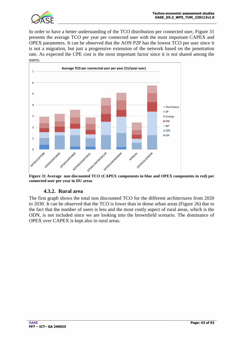
Techno-economic assessment studies OASE_D5.3_WP5_TUM_220113v1.0
OASE FP7 – ICT– GA 249025
Page: 43 of 92
In order to have a better understanding of the TCO distribution per connected user, Figure 31
presents the average TCO per year per connected user with the most important CAPEX and
OPEX parameters. It can be observed that the AON P2P has the lowest TCO per user since it
is not a migration, but just a progressive extension of the network based on the penetration
rate. As expected the CPE cost is the most important factor since it is not shared among the
users.
Figure 31 Average non discounted TCO (CAPEX components in blue and OPEX components in red) per
connected user per year in DU areas
4.3.2. Rural area
The first graph shows the total non discounted TCO for the different architectures from 2020
to 2030. It can be observed that the TCO is lower than in dense urban areas (Figure 26) due to
the fact that the number of users is less and the most costly aspect of rural areas, which is the
ODN, is not included since we are looking into the brownfield scenario. The dominance of
OPEX over CAPEX is kept also in rural areas.
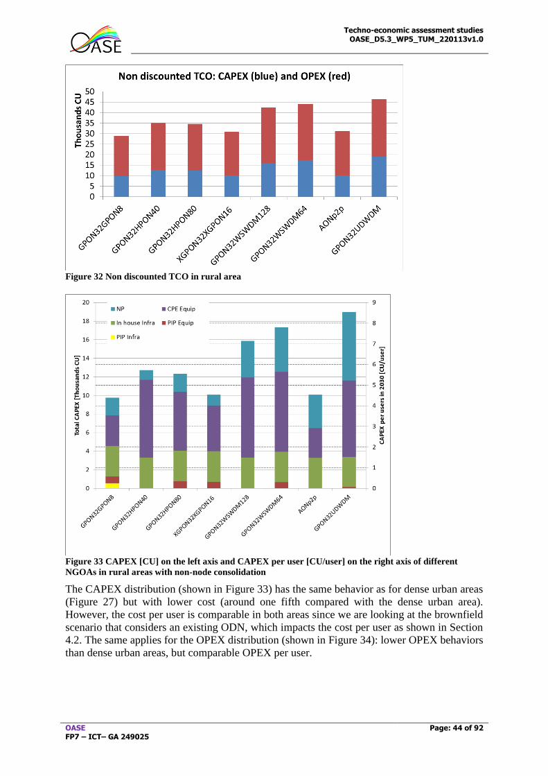
Techno-economic assessment studies OASE_D5.3_WP5_TUM_220113v1.0
OASE FP7 – ICT– GA 249025
Page: 44 of 92
Figure 32 Non discounted TCO in rural area
Figure 33 CAPEX [CU] on the left axis and CAPEX per user [CU/user] on the right axis of different
NGOAs in rural areas with non-node consolidation
The CAPEX distribution (shown in Figure 33) has the same behavior as for dense urban areas
(Figure 27) but with lower cost (around one fifth compared with the dense urban area).
However, the cost per user is comparable in both areas since we are looking at the brownfield
scenario that considers an existing ODN, which impacts the cost per user as shown in Section
4.2. The same applies for the OPEX distribution (shown in Figure 34): lower OPEX behaviors
than dense urban areas, but comparable OPEX per user.
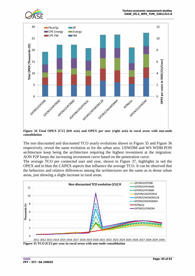
Techno-economic assessment studies OASE_D5.3_WP5_TUM_220113v1.0
OASE FP7 – ICT– GA 249025
Page: 45 of 92
Figure 34 Total OPEX [CU] (left axis) and OPEX per user (right axis) in rural areas with non-node
consolidation
The non discounted and discounted TCO yearly evolutions shown in Figure 35 and Figure 36
respectively, reveal the same evolution as for the urban area. UDWDM and WS WDM PON
architecture keep being the architecture requiring the highest investment at the migration.
AON P2P keeps the increasing investment curve based on the penetration curve.
The average TCO per connected user and year, shown in Figure 37, highlights in red the
OPEX and in blue the CAPEX aspects that influence the average TCO. It can be observed that
the behaviors and relative differences among the architectures are the same as in dense urban
areas, just showing a slight increase in rural areas.
Figure 35 TCO [CU] per year in rural areas with non-node consolidation
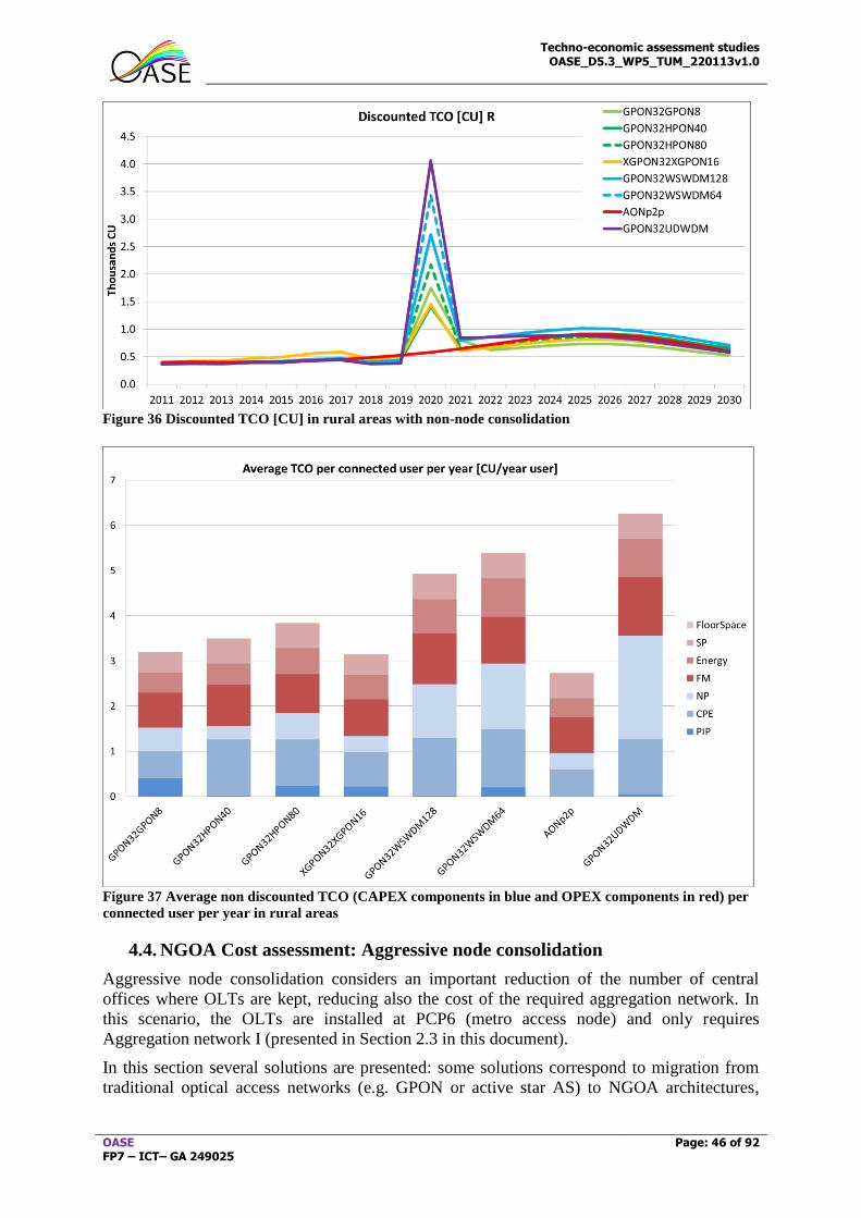
Techno-economic assessment studies OASE_D5.3_WP5_TUM_220113v1.0
OASE FP7 – ICT– GA 249025
Page: 46 of 92
Figure 36 Discounted TCO [CU] in rural areas with non-node consolidation
Figure 37 Average non discounted TCO (CAPEX components in blue and OPEX components in red) per
connected user per year in rural areas
4.4. NGOA Cost assessment: Aggressive node consolidation
Aggressive node consolidation considers an important reduction of the number of central
offices where OLTs are kept, reducing also the cost of the required aggregation network. In
this scenario, the OLTs are installed at PCP6 (metro access node) and only requires
Aggregation network I (presented in Section 2.3 in this document).
In this section several solutions are presented: some solutions correspond to migration from
traditional optical access networks (e.g. GPON or active star AS) to NGOA architectures,
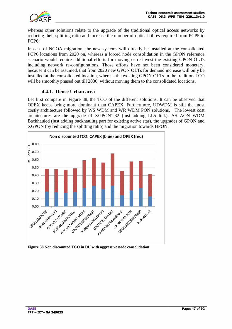
Techno-economic assessment studies OASE_D5.3_WP5_TUM_220113v1.0
OASE FP7 – ICT– GA 249025
Page: 47 of 92
whereas other solutions relate to the upgrade of the traditional optical access networks by
reducing their splitting ratio and increase the number of optical fibres required from PCP5 to
PCP6.
In case of NGOA migration, the new systems will directly be installed at the consolidated
PCP6 locations from 2020 on, whereas a forced node consolidation in the GPON reference
scenario would require additional efforts for moving or re-invest the existing GPON OLTs
including network re-configurations. Those efforts have not been considered monetary,
because it can be assumed, that from 2020 new GPON OLTs for demand increase will only be
installed at the consolidated location, whereas the existing GPON OLTs in the traditional CO
will be smoothly phased out till 2030, without moving them to the consolidated locations.
4.4.1. Dense Urban area
Let first compare in Figure 38, the TCO of the different solutions. It can be observed that
OPEX keeps being more dominant than CAPEX. Furthermore, UDWDM is still the most
costly architecture followed by WS WDM and WR WDM PON solutions. The lowest cost
architectures are the upgrade of XGPON1:32 (just adding LL5 link), AS AON WDM
Backhauled (just adding backhauling part for existing active star), the upgrades of GPON and
XGPON (by reducing the splitting ratio) and the migration towards HPON.
Figure 38 Non discounted TCO in DU with aggressive node consolidation
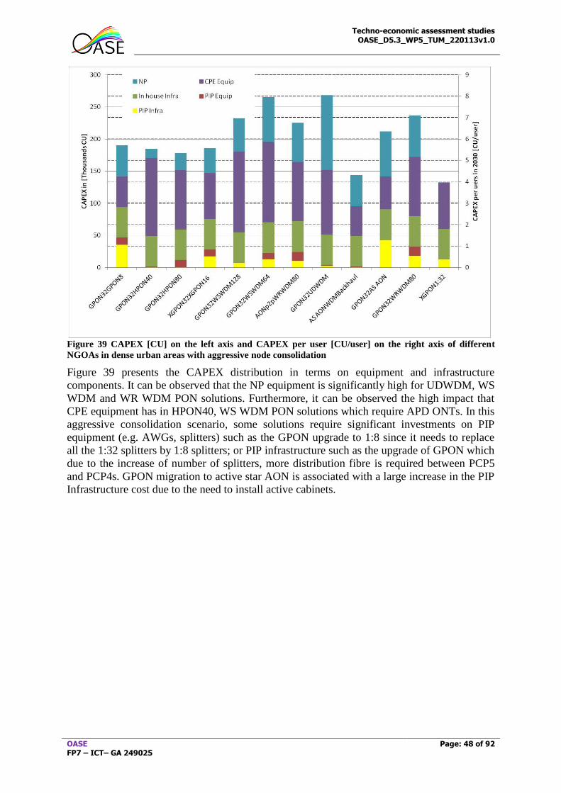
Techno-economic assessment studies OASE_D5.3_WP5_TUM_220113v1.0
OASE FP7 – ICT– GA 249025
Page: 48 of 92
Figure 39 CAPEX [CU] on the left axis and CAPEX per user [CU/user] on the right axis of different
NGOAs in dense urban areas with aggressive node consolidation
Figure 39 presents the CAPEX distribution in terms on equipment and infrastructure
components. It can be observed that the NP equipment is significantly high for UDWDM, WS
WDM and WR WDM PON solutions. Furthermore, it can be observed the high impact that
CPE equipment has in HPON40, WS WDM PON solutions which require APD ONTs. In this
aggressive consolidation scenario, some solutions require significant investments on PIP
equipment (e.g. AWGs, splitters) such as the GPON upgrade to 1:8 since it needs to replace
all the 1:32 splitters by 1:8 splitters; or PIP infrastructure such as the upgrade of GPON which
due to the increase of number of splitters, more distribution fibre is required between PCP5
and PCP4s. GPON migration to active star AON is associated with a large increase in the PIP
Infrastructure cost due to the need to install active cabinets.
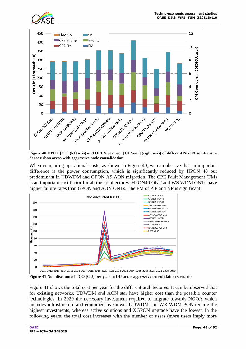
Techno-economic assessment studies OASE_D5.3_WP5_TUM_220113v1.0
OASE FP7 – ICT– GA 249025
Page: 49 of 92
Figure 40 OPEX [CU] (left axis) and OPEX per user [CU/user] (right axis) of different NGOA solutions in
dense urban areas with aggressive node consolidation
When comparing operational costs, as shown in Figure 40, we can observe that an important
difference is the power consumption, which is significantly reduced by HPON 40 but
predominant in UDWDM and GPON AS AON migration. The CPE Fault Management (FM)
is an important cost factor for all the architectures: HPON40 ONT and WS WDM ONTs have
higher failure rates than GPON and AON ONTs. The FM of PIP and NP is significant.
Figure 41 Non discounted TCO [CU] per year in DU areas aggressive consolidation scenario
Figure 41 shows the total cost per year for the different architectures. It can be observed that
for existing networks, UDWDM and AON star have higher cost than the possible counter
technologies. In 2020 the necessary investment required to migrate towards NGOA which
includes infrastructure and equipment is shown: UDWDM and WR WDM PON require the
highest investments, whereas active solutions and XGPON upgrade have the lowest. In the
following years, the total cost increases with the number of users (more users imply more
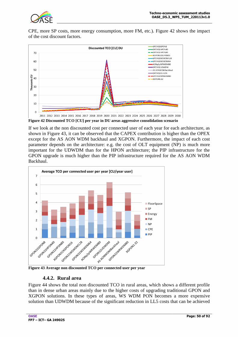
Techno-economic assessment studies OASE_D5.3_WP5_TUM_220113v1.0
OASE FP7 – ICT– GA 249025
Page: 50 of 92
CPE, more SP costs, more energy consumption, more FM, etc.). Figure 42 shows the impact
of the cost discount factors.
Figure 42 Discounted TCO [CU] per year in DU areas aggressive consolidation scenario
If we look at the non discounted cost per connected user of each year for each architecture, as
shown in Figure 43, it can be observed that the CAPEX contribution is higher than the OPEX
except for the AS AON WDM backhaul and XGPON. Furthermore, the impact of each cost
parameter depends on the architecture: e.g. the cost of OLT equipment (NP) is much more
important for the UDWDM than for the HPON architecture; the PIP infrastructure for the
GPON upgrade is much higher than the PIP infrastructure required for the AS AON WDM
Backhaul.
Figure 43 Average non discounted TCO per connected user per year
4.4.2. Rural area
Figure 44 shows the total non discounted TCO in rural areas, which shows a different profile
than in dense urban areas mainly due to the higher costs of upgrading traditional GPON and
XGPON solutions. In these types of areas, WS WDM PON becomes a more expensive
solution than UDWDM because of the significant reduction in LL5 costs that can be achieved
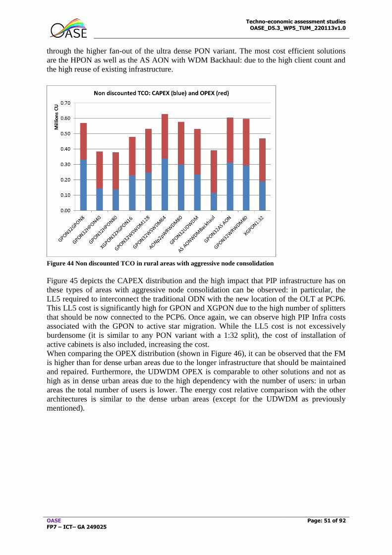
Techno-economic assessment studies OASE_D5.3_WP5_TUM_220113v1.0
OASE FP7 – ICT– GA 249025
Page: 51 of 92
through the higher fan-out of the ultra dense PON variant. The most cost efficient solutions
are the HPON as well as the AS AON with WDM Backhaul: due to the high client count and
the high reuse of existing infrastructure.
Figure 44 Non discounted TCO in rural areas with aggressive node consolidation
Figure 45 depicts the CAPEX distribution and the high impact that PIP infrastructure has on
these types of areas with aggressive node consolidation can be observed: in particular, the
LL5 required to interconnect the traditional ODN with the new location of the OLT at PCP6.
This LL5 cost is significantly high for GPON and XGPON due to the high number of splitters
that should be now connected to the PCP6. Once again, we can observe high PIP Infra costs
associated with the GPON to active star migration. While the LL5 cost is not excessively
burdensome (it is similar to any PON variant with a 1:32 split), the cost of installation of
active cabinets is also included, increasing the cost.
When comparing the OPEX distribution (shown in Figure 46), it can be observed that the FM
is higher than for dense urban areas due to the longer infrastructure that should be maintained
and repaired. Furthermore, the UDWDM OPEX is comparable to other solutions and not as
high as in dense urban areas due to the high dependency with the number of users: in urban
areas the total number of users is lower. The energy cost relative comparison with the other
architectures is similar to the dense urban areas (except for the UDWDM as previously
mentioned).
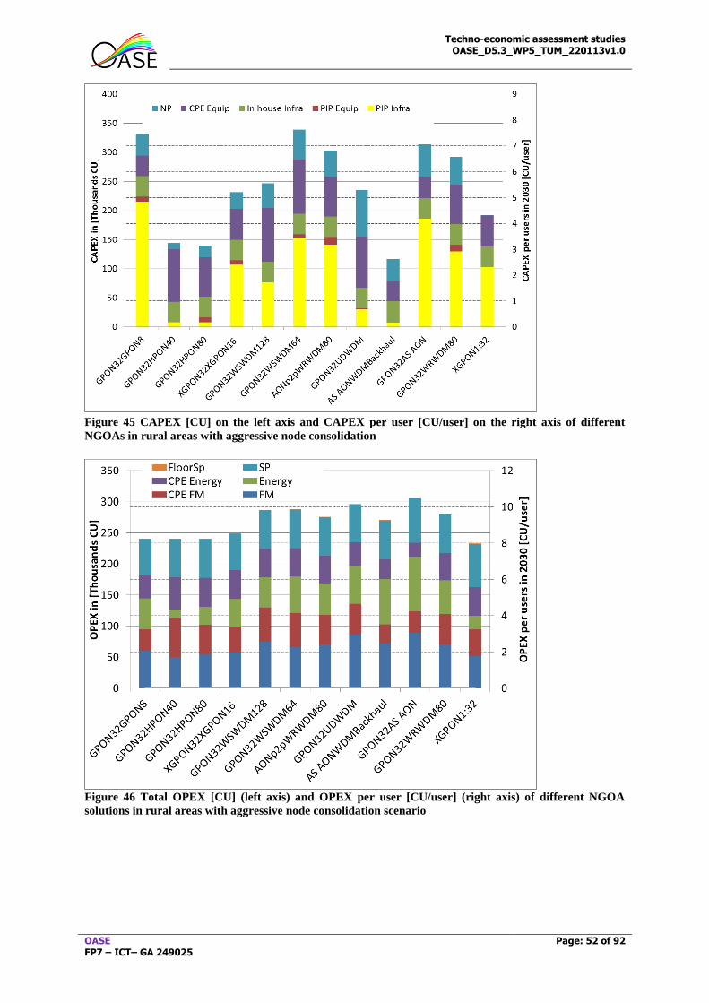
Techno-economic assessment studies OASE_D5.3_WP5_TUM_220113v1.0
OASE FP7 – ICT– GA 249025
Page: 52 of 92
Figure 45 CAPEX [CU] on the left axis and CAPEX per user [CU/user] on the right axis of different
NGOAs in rural areas with aggressive node consolidation
Figure 46 Total OPEX [CU] (left axis) and OPEX per user [CU/user] (right axis) of different NGOA
solutions in rural areas with aggressive node consolidation scenario
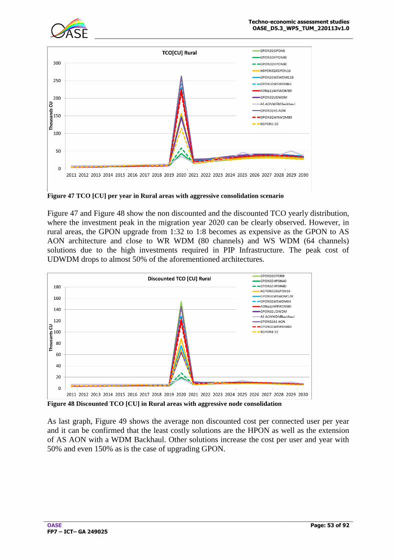
Techno-economic assessment studies OASE_D5.3_WP5_TUM_220113v1.0
OASE FP7 – ICT– GA 249025
Page: 53 of 92
Figure 47 TCO [CU] per year in Rural areas with aggressive consolidation scenario
Figure 47 and Figure 48 show the non discounted and the discounted TCO yearly distribution,
where the investment peak in the migration year 2020 can be clearly observed. However, in
rural areas, the GPON upgrade from 1:32 to 1:8 becomes as expensive as the GPON to AS
AON architecture and close to WR WDM (80 channels) and WS WDM (64 channels)
solutions due to the high investments required in PIP Infrastructure. The peak cost of
UDWDM drops to almost 50% of the aforementioned architectures.
Figure 48 Discounted TCO [CU] in Rural areas with aggressive node consolidation
As last graph, Figure 49 shows the average non discounted cost per connected user per year
and it can be confirmed that the least costly solutions are the HPON as well as the extension
of AS AON with a WDM Backhaul. Other solutions increase the cost per user and year with
50% and even 150% as is the case of upgrading GPON.
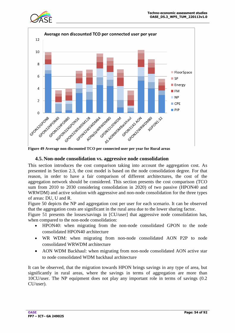
Techno-economic assessment studies OASE_D5.3_WP5_TUM_220113v1.0
OASE FP7 – ICT– GA 249025
Page: 54 of 92
Figure 49 Average non discounted TCO per connected user per year for Rural areas
4.5. Non-node consolidation vs. aggressive node consolidation
This section introduces the cost comparison taking into account the aggregation cost. As
presented in Section 2.3, the cost model is based on the node consolidation degree. For that
reason, in order to have a fair comparison of different architectures, the cost of the
aggregation network should be considered. This section presents the cost comparison (TCO
sum from 2010 to 2030 considering consolidation in 2020) of two passive (HPON40 and
WRWDM) and active solution with aggressive and non-node consolidation for the three types
of areas: DU, U and R.
Figure 50 depicts the NP and aggregation cost per user for each scenario. It can be observed
that the aggregation costs are significant in the rural area due to the lower sharing factor.
Figure 51 presents the losses/savings in [CU/user] that aggressive node consolidation has,
when compared to the non-node consolidation:
HPON40: when migrating from the non-node consolidated GPON to the node
consolidated HPON40 architecture
WR WDM: when migrating from non-node consolidated AON P2P to node
consolidated WRWDM architecture
AON WDM Backhaul: when migrating from non-node consolidated AON active star
to node consolidated WDM backhaul architecture
It can be observed, that the migration towards HPON brings savings in any type of area, but
significantly in rural areas, where the savings in terms of aggregation are more than
10CU/user. The NP equipment does not play any important role in terms of savings (0.2
CU/user).
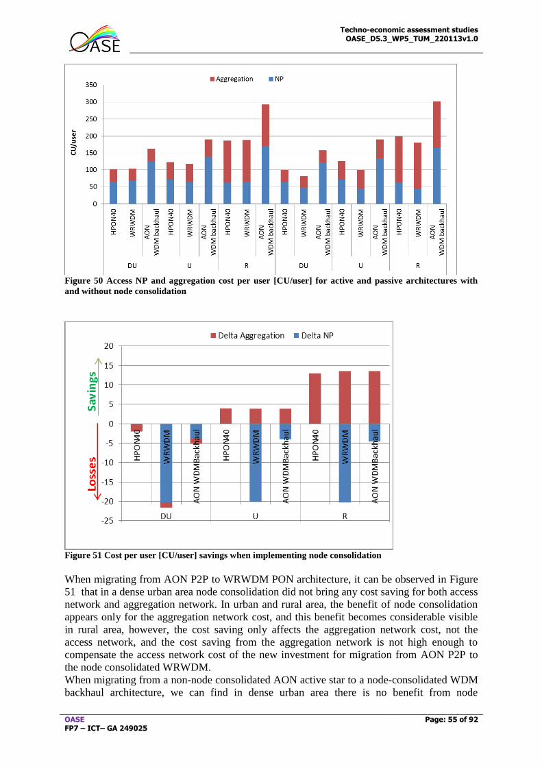
Techno-economic assessment studies OASE_D5.3_WP5_TUM_220113v1.0
OASE FP7 – ICT– GA 249025
Page: 55 of 92
Figure 50 Access NP and aggregation cost per user [CU/user] for active and passive architectures with
and without node consolidation
Figure 51 Cost per user [CU/user] savings when implementing node consolidation
When migrating from AON P2P to WRWDM PON architecture, it can be observed in Figure
51 that in a dense urban area node consolidation did not bring any cost saving for both access
network and aggregation network. In urban and rural area, the benefit of node consolidation
appears only for the aggregation network cost, and this benefit becomes considerable visible
in rural area, however, the cost saving only affects the aggregation network cost, not the
access network, and the cost saving from the aggregation network is not high enough to
compensate the access network cost of the new investment for migration from AON P2P to
the node consolidated WRWDM.
When migrating from a non-node consolidated AON active star to a node-consolidated WDM
backhaul architecture, we can find in dense urban area there is no benefit from node
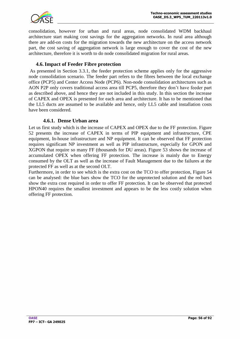
Techno-economic assessment studies OASE_D5.3_WP5_TUM_220113v1.0
OASE FP7 – ICT– GA 249025
Page: 56 of 92
consolidation, however for urban and rural areas, node consolidated WDM backhaul
architecture start making cost savings for the aggregation networks. In rural area although
there are add-on costs for the migration towards the new architecture on the access network
part, the cost saving of aggregation network is large enough to cover the cost of the new
architecture, therefore it is worth to do node consolidated migration for rural areas.
4.6. Impact of Feeder Fibre protection
As presented in Section 3.3.1, the feeder protection scheme applies only for the aggressive
node consolidation scenario. The feeder part refers to the fibres between the local exchange
office (PCP5) and Center Access Node (PCP6). Non-node consolidation architectures such as
AON P2P only covers traditional access area till PCP5, therefore they don’t have feeder part
as described above, and hence they are not included in this study. In this section the increase
of CAPEX and OPEX is presented for each area and architecture. It has to be mentioned that
the LL5 ducts are assumed to be available and hence, only LL5 cable and installation costs
have been considered.
4.6.1. Dense Urban area
Let us first study which is the increase of CAPEX and OPEX due to the FF protection. Figure
52 presents the increase of CAPEX in terms of PIP equipment and infrastructure, CPE
equipment, In-house infrastructure and NP equipment. It can be observed that FF protection
requires significant NP investment as well as PIP infrastructure, especially for GPON and
XGPON that require so many FF (thousands for DU areas). Figure 53 shows the increase of
accumulated OPEX when offering FF protection. The increase is mainly due to Energy
consumed by the OLT as well as the increase of Fault Management due to the failures at the
protected FF as well as at the second OLT.
Furthermore, in order to see which is the extra cost on the TCO to offer protection, Figure 54
can be analysed: the blue bars show the TCO for the unprotected solution and the red bars
show the extra cost required in order to offer FF protection. It can be observed that protected
HPON40 requires the smallest investment and appears to be the less costly solution when
offering FF protection.
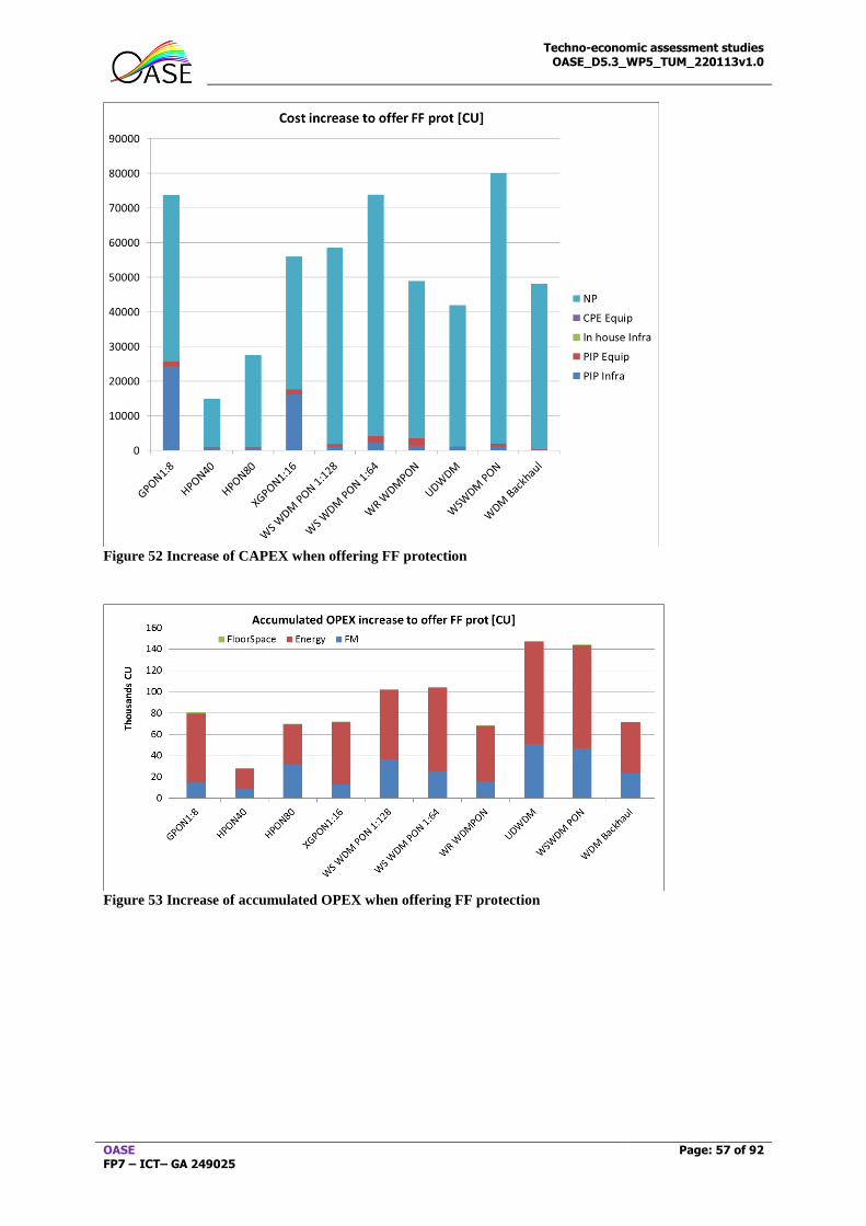
Techno-economic assessment studies OASE_D5.3_WP5_TUM_220113v1.0
OASE FP7 – ICT– GA 249025
Page: 57 of 92
Figure 52 Increase of CAPEX when offering FF protection
Figure 53 Increase of accumulated OPEX when offering FF protection
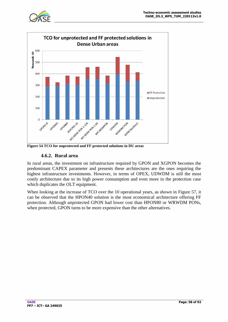
Techno-economic assessment studies OASE_D5.3_WP5_TUM_220113v1.0
OASE FP7 – ICT– GA 249025
Page: 58 of 92
Figure 54 TCO for unprotected and FF protected solutions in DU areas
4.6.2. Rural area
In rural areas, the investment on infrastructure required by GPON and XGPON becomes the
predominant CAPEX parameter and presents these architectures are the ones requiring the
highest infrastructure investments. However, in terms of OPEX, UDWDM is still the most
costly architecture due to its high power consumption and even more in the protection case
which duplicates the OLT equipment.
When looking at the increase of TCO over the 10 operational years, as shown in Figure 57, it
can be observed that the HPON40 solution is the most economical architecture offering FF
protection. Although unprotected GPON had lower cost than HPON80 or WRWDM PONs,
when protected, GPON turns to be more expensive than the other alternatives.
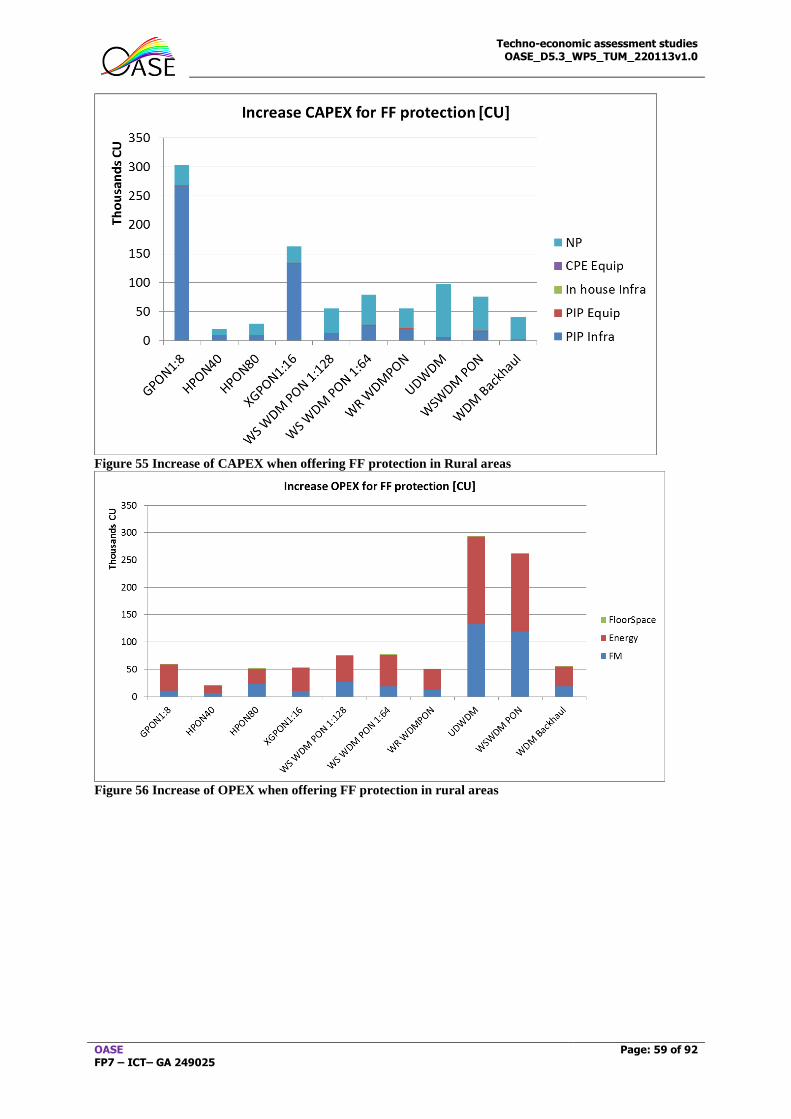
Techno-economic assessment studies OASE_D5.3_WP5_TUM_220113v1.0
OASE FP7 – ICT– GA 249025
Page: 59 of 92
Figure 55 Increase of CAPEX when offering FF protection in Rural areas
Figure 56 Increase of OPEX when offering FF protection in rural areas
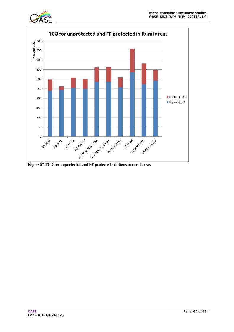
Techno-economic assessment studies OASE_D5.3_WP5_TUM_220113v1.0
OASE FP7 – ICT– GA 249025
Page: 60 of 92
Figure 57 TCO for unprotected and FF protected solutions in rural areas
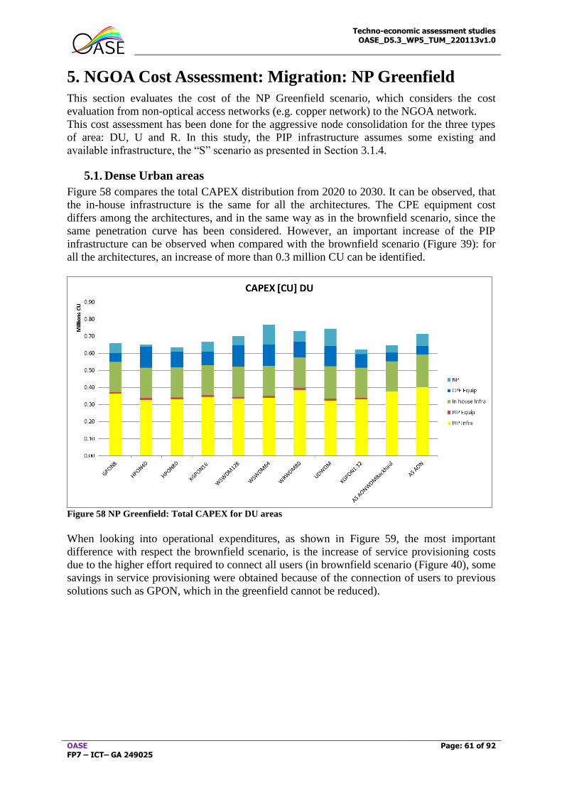
Techno-economic assessment studies OASE_D5.3_WP5_TUM_220113v1.0
OASE FP7 – ICT– GA 249025
Page: 61 of 92
5. NGOA Cost Assessment: Migration: NP Greenfield
This section evaluates the cost of the NP Greenfield scenario, which considers the cost
evaluation from non-optical access networks (e.g. copper network) to the NGOA network.
This cost assessment has been done for the aggressive node consolidation for the three types
of area: DU, U and R. In this study, the PIP infrastructure assumes some existing and
available infrastructure, the “S” scenario as presented in Section 3.1.4.
5.1. Dense Urban areas
Figure 58 compares the total CAPEX distribution from 2020 to 2030. It can be observed, that
the in-house infrastructure is the same for all the architectures. The CPE equipment cost
differs among the architectures, and in the same way as in the brownfield scenario, since the
same penetration curve has been considered. However, an important increase of the PIP
infrastructure can be observed when compared with the brownfield scenario (Figure 39): for
all the architectures, an increase of more than 0.3 million CU can be identified.
Figure 58 NP Greenfield: Total CAPEX for DU areas
When looking into operational expenditures, as shown in Figure 59, the most important
difference with respect the brownfield scenario, is the increase of service provisioning costs
due to the higher effort required to connect all users (in brownfield scenario (Figure 40), some
savings in service provisioning were obtained because of the connection of users to previous
solutions such as GPON, which in the greenfield cannot be reduced).
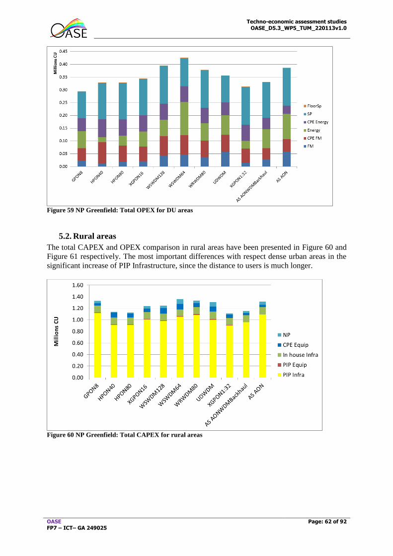
Techno-economic assessment studies OASE_D5.3_WP5_TUM_220113v1.0
OASE FP7 – ICT– GA 249025
Page: 62 of 92
Figure 59 NP Greenfield: Total OPEX for DU areas
5.2. Rural areas
The total CAPEX and OPEX comparison in rural areas have been presented in Figure 60 and
Figure 61 respectively. The most important differences with respect dense urban areas in the
significant increase of PIP Infrastructure, since the distance to users is much longer.
Figure 60 NP Greenfield: Total CAPEX for rural areas
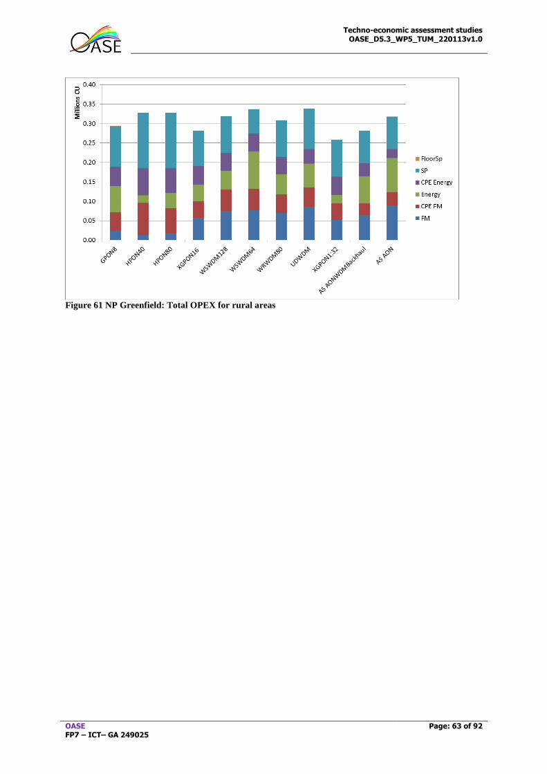
Techno-economic assessment studies OASE_D5.3_WP5_TUM_220113v1.0
OASE FP7 – ICT– GA 249025
Page: 63 of 92
Figure 61 NP Greenfield: Total OPEX for rural areas
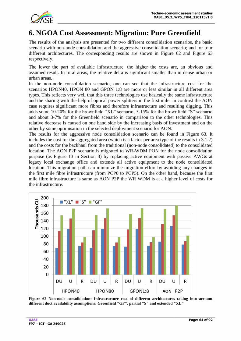
Techno-economic assessment studies OASE_D5.3_WP5_TUM_220113v1.0
OASE FP7 – ICT– GA 249025
Page: 64 of 92
6. NGOA Cost Assessment: Migration: Pure Greenfield
The results of the analysis are presented for two different consolidation scenarios, the basic
scenario with non-node consolidation and the aggressive consolidation scenario; and for four
different architectures. The corresponding results are shown in Figure 62 and Figure 63
respectively.
The lower the part of available infrastructure, the higher the costs are, an obvious and
assumed result. In rural areas, the relative delta is significant smaller than in dense urban or
urban areas.
In the non-node consolidation scenario, one can see that the infrastructure cost for the
scenarios HPON40, HPON 80 and GPON 1:8 are more or less similar in all different area
types. This reflects very well that this three technologies use basically the same infrastructure
and the sharing with the help of optical power splitters in the first mile. In contrast the AON
case requires significant more fibres and therefore infrastructure and resulting digging. This
adds some 10-20% for the brownfield “XL” scenario, 5-15% for the brownfield “S” scenario
and about 3-7% for the Greenfield scenario in comparison to the other technologies. This
relative decrease is caused on one hand side by the increasing basis of investment and on the
other by some optimisation in the selected deployment scenario for AON.
The results for the aggressive node consolidation scenario can be found in Figure 63. It
includes the cost for the aggregated area (which is a factor per area type of the results in 3.1.2)
and the costs for the backhaul from the traditional (non-node consolidated) to the consolidated
location. The AON P2P scenario is migrated to WR-WDM PON for the node consolidation
purpose (as Figure 13 in Section 3) by replacing active equipment with passive AWGs at
legacy local exchange office and extends all active equipment to the node consolidated
location. This migration path can minimize the migration effort by avoiding any changes in
the first mile fibre infrastructure (from PCP0 to PCP5). On the other hand, because the first
mile fibre infrastructure is same as AON P2P the WR WDM is at a higher level of costs for
the infrastructure.
Figure 62 Non-node consolidation: Infrastructure cost of different architectures taking into account
different duct availability assumptions: Greenfield "GF", partial "S" and extended "XL"
AON
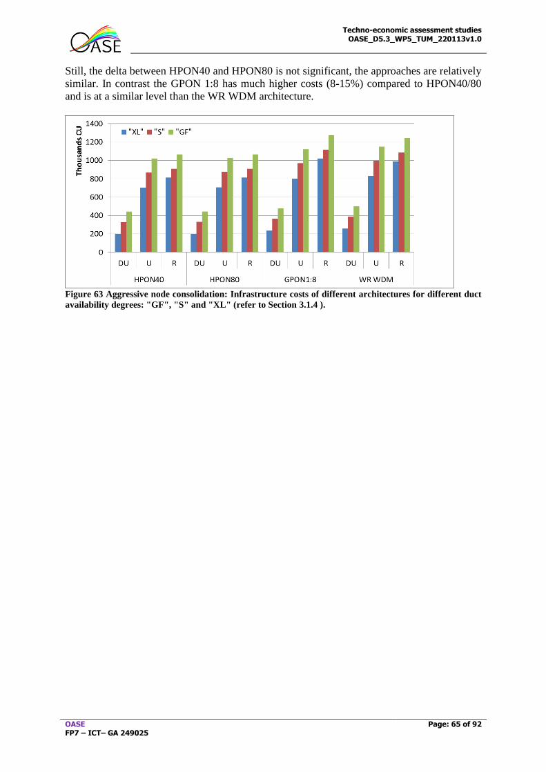
Techno-economic assessment studies OASE_D5.3_WP5_TUM_220113v1.0
OASE FP7 – ICT– GA 249025
Page: 65 of 92
Still, the delta between HPON40 and HPON80 is not significant, the approaches are relatively
similar. In contrast the GPON 1:8 has much higher costs (8-15%) compared to HPON40/80
and is at a similar level than the WR WDM architecture.
Figure 63 Aggressive node consolidation: Infrastructure costs of different architectures for different duct
availability degrees: "GF", "S" and "XL" (refer to Section 3.1.4 ).
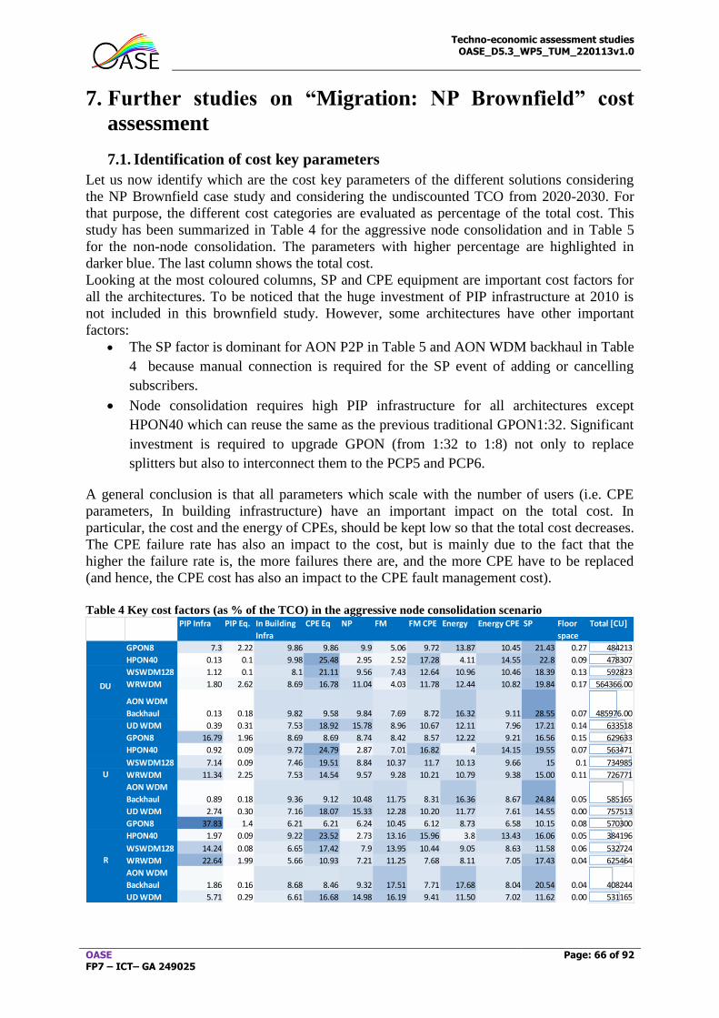
Techno-economic assessment studies OASE_D5.3_WP5_TUM_220113v1.0
OASE FP7 – ICT– GA 249025
Page: 66 of 92
7. Further studies on “Migration: NP Brownfield” cost
assessment
7.1. Identification of cost key parameters
Let us now identify which are the cost key parameters of the different solutions considering
the NP Brownfield case study and considering the undiscounted TCO from 2020-2030. For
that purpose, the different cost categories are evaluated as percentage of the total cost. This
study has been summarized in Table 4 for the aggressive node consolidation and in Table 5
for the non-node consolidation. The parameters with higher percentage are highlighted in
darker blue. The last column shows the total cost.
Looking at the most coloured columns, SP and CPE equipment are important cost factors for
all the architectures. To be noticed that the huge investment of PIP infrastructure at 2010 is
not included in this brownfield study. However, some architectures have other important
factors:
The SP factor is dominant for AON P2P in Table 5 and AON WDM backhaul in Table
4 because manual connection is required for the SP event of adding or cancelling
subscribers.
Node consolidation requires high PIP infrastructure for all architectures except
HPON40 which can reuse the same as the previous traditional GPON1:32. Significant
investment is required to upgrade GPON (from 1:32 to 1:8) not only to replace
splitters but also to interconnect them to the PCP5 and PCP6.
A general conclusion is that all parameters which scale with the number of users (i.e. CPE
parameters, In building infrastructure) have an important impact on the total cost. In
particular, the cost and the energy of CPEs, should be kept low so that the total cost decreases.
The CPE failure rate has also an impact to the cost, but is mainly due to the fact that the
higher the failure rate is, the more failures there are, and the more CPE have to be replaced
(and hence, the CPE cost has also an impact to the CPE fault management cost).
Table 4 Key cost factors (as % of the TCO) in the aggressive node consolidation scenario
PIP Infra PIP Eq. In Building
Infra
CPE Eq NP FM FM CPE Energy Energy CPE SP Floor
space
Total [CU]
GPON8 7.3 2.22 9.86 9.86 9.9 5.06 9.72 13.87 10.45 21.43 0.27 484213
HPON40 0.13 0.1 9.98 25.48 2.95 2.52 17.28 4.11 14.55 22.8 0.09 478307
WSWDM128 1.12 0.1 8.1 21.11 9.56 7.43 12.64 10.96 10.46 18.39 0.13 592823
WRWDM 1.80 2.62 8.69 16.78 11.04 4.03 11.78 12.44 10.82 19.84 0.17 564366.00
AON WDM
Backhaul 0.13 0.18 9.82 9.58 9.84 7.69 8.72 16.32 9.11 28.55 0.07 485976.00
UD WDM 0.39 0.31 7.53 18.92 15.78 8.96 10.67 12.11 7.96 17.21 0.14 633518
GPON8 16.79 1.96 8.69 8.69 8.74 8.42 8.57 12.22 9.21 16.56 0.15 629633
HPON40 0.92 0.09 9.72 24.79 2.87 7.01 16.82 4 14.15 19.55 0.07 563471
WSWDM128 7.14 0.09 7.46 19.51 8.84 10.37 11.7 10.13 9.66 15 0.1 734985
WRWDM 11.34 2.25 7.53 14.54 9.57 9.28 10.21 10.79 9.38 15.00 0.11 726771
AON WDM
Backhaul 0.89 0.18 9.36 9.12 10.48 11.75 8.31 16.36 8.67 24.84 0.05 585165
UD WDM 2.74 0.30 7.16 18.07 15.33 12.28 10.20 11.77 7.61 14.55 0.00 757513
GPON8 37.83 1.4 6.21 6.21 6.24 10.45 6.12 8.73 6.58 10.15 0.08 570300
HPON40 1.97 0.09 9.22 23.52 2.73 13.16 15.96 3.8 13.43 16.06 0.05 384196
WSWDM128 14.24 0.08 6.65 17.42 7.9 13.95 10.44 9.05 8.63 11.58 0.06 532724
WRWDM 22.64 1.99 5.66 10.93 7.21 11.25 7.68 8.11 7.05 17.43 0.04 625464
AON WDM
Backhaul 1.86 0.16 8.68 8.46 9.32 17.51 7.71 17.68 8.04 20.54 0.04 408244
UD WDM 5.71 0.29 6.61 16.68 14.98 16.19 9.41 11.50 7.02 11.62 0.00 531165
DU
U
R
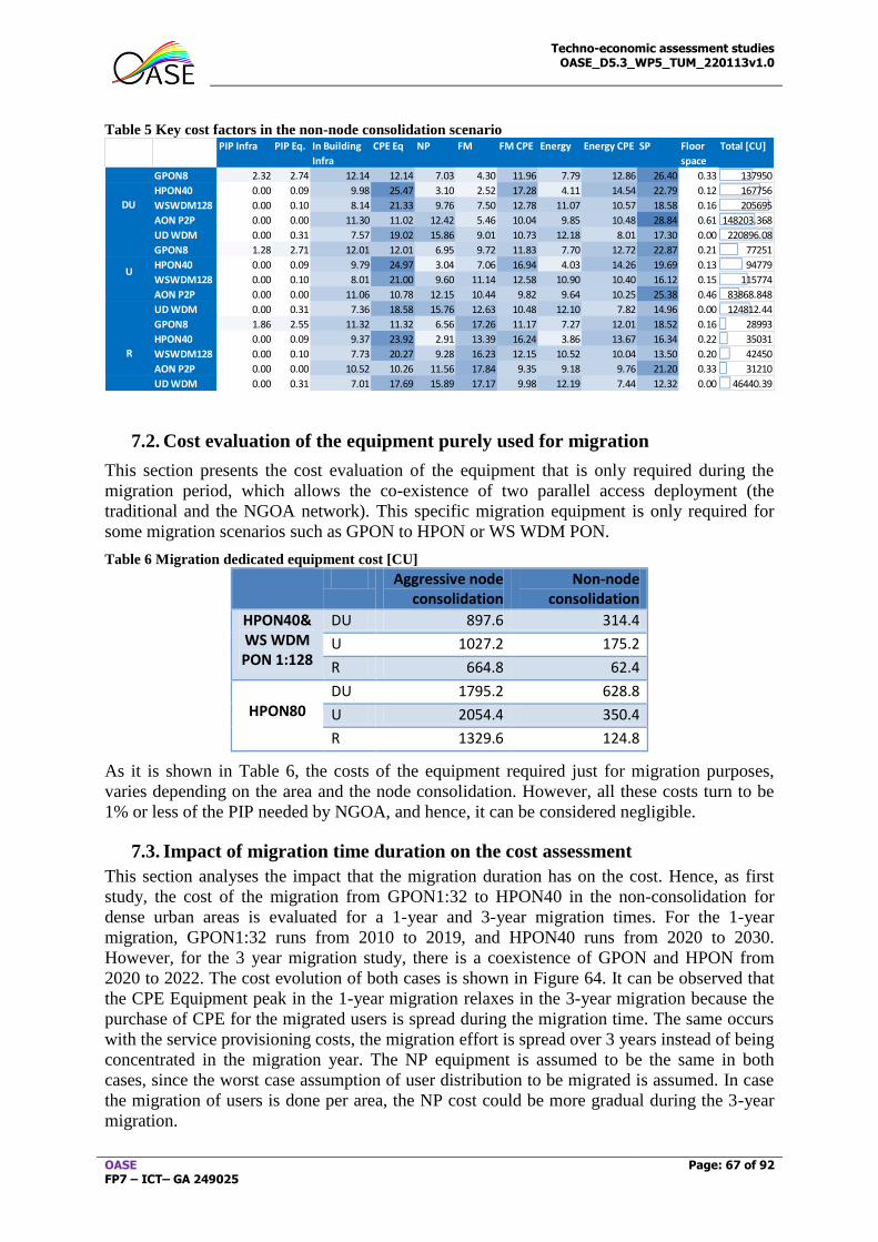
Techno-economic assessment studies OASE_D5.3_WP5_TUM_220113v1.0
OASE FP7 – ICT– GA 249025
Page: 67 of 92
Table 5 Key cost factors in the non-node consolidation scenario
7.2. Cost evaluation of the equipment purely used for migration
This section presents the cost evaluation of the equipment that is only required during the
migration period, which allows the co-existence of two parallel access deployment (the
traditional and the NGOA network). This specific migration equipment is only required for
some migration scenarios such as GPON to HPON or WS WDM PON.
Table 6 Migration dedicated equipment cost [CU]
Aggressive node consolidation
Non-node consolidation
HPON40& WS WDM PON 1:128
DU 897.6 314.4
U 1027.2 175.2
R 664.8 62.4
HPON80
DU 1795.2 628.8
U 2054.4 350.4
R 1329.6 124.8
As it is shown in Table 6, the costs of the equipment required just for migration purposes,
varies depending on the area and the node consolidation. However, all these costs turn to be
1% or less of the PIP needed by NGOA, and hence, it can be considered negligible.
7.3. Impact of migration time duration on the cost assessment
This section analyses the impact that the migration duration has on the cost. Hence, as first
study, the cost of the migration from GPON1:32 to HPON40 in the non-consolidation for
dense urban areas is evaluated for a 1-year and 3-year migration times. For the 1-year
migration, GPON1:32 runs from 2010 to 2019, and HPON40 runs from 2020 to 2030.
However, for the 3 year migration study, there is a coexistence of GPON and HPON from
2020 to 2022. The cost evolution of both cases is shown in Figure 64. It can be observed that
the CPE Equipment peak in the 1-year migration relaxes in the 3-year migration because the
purchase of CPE for the migrated users is spread during the migration time. The same occurs
with the service provisioning costs, the migration effort is spread over 3 years instead of being
concentrated in the migration year. The NP equipment is assumed to be the same in both
cases, since the worst case assumption of user distribution to be migrated is assumed. In case
the migration of users is done per area, the NP cost could be more gradual during the 3-year
migration.
PIP Infra PIP Eq. In Building
Infra
CPE Eq NP FM FM CPE Energy Energy CPE SP Floor
space
Total [CU]
GPON8 2.32 2.74 12.14 12.14 7.03 4.30 11.96 7.79 12.86 26.40 0.33 137950
HPON40 0.00 0.09 9.98 25.47 3.10 2.52 17.28 4.11 14.54 22.79 0.12 167756
WSWDM128 0.00 0.10 8.14 21.33 9.76 7.50 12.78 11.07 10.57 18.58 0.16 205695
AON P2P 0.00 0.00 11.30 11.02 12.42 5.46 10.04 9.85 10.48 28.84 0.61 148203.368
UD WDM 0.00 0.31 7.57 19.02 15.86 9.01 10.73 12.18 8.01 17.30 0.00 220896.08
GPON8 1.28 2.71 12.01 12.01 6.95 9.72 11.83 7.70 12.72 22.87 0.21 77251
HPON40 0.00 0.09 9.79 24.97 3.04 7.06 16.94 4.03 14.26 19.69 0.13 94779
WSWDM128 0.00 0.10 8.01 21.00 9.60 11.14 12.58 10.90 10.40 16.12 0.15 115774
AON P2P 0.00 0.00 11.06 10.78 12.15 10.44 9.82 9.64 10.25 25.38 0.46 83868.848
UD WDM 0.00 0.31 7.36 18.58 15.76 12.63 10.48 12.10 7.82 14.96 0.00 124812.44
GPON8 1.86 2.55 11.32 11.32 6.56 17.26 11.17 7.27 12.01 18.52 0.16 28993
HPON40 0.00 0.09 9.37 23.92 2.91 13.39 16.24 3.86 13.67 16.34 0.22 35031
WSWDM128 0.00 0.10 7.73 20.27 9.28 16.23 12.15 10.52 10.04 13.50 0.20 42450
AON P2P 0.00 0.00 10.52 10.26 11.56 17.84 9.35 9.18 9.76 21.20 0.33 31210
UD WDM 0.00 0.31 7.01 17.69 15.89 17.17 9.98 12.19 7.44 12.32 0.00 46440.39
U
DU
R
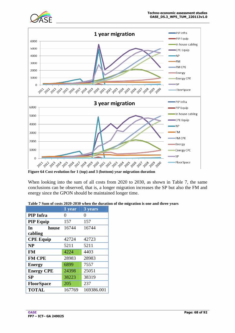
Techno-economic assessment studies OASE_D5.3_WP5_TUM_220113v1.0
OASE FP7 – ICT– GA 249025
Page: 68 of 92
Figure 64 Cost evolution for 1 (top) and 3 (bottom) year migration duration
When looking into the sum of all costs from 2020 to 2030, as shown in Table 7, the same
conclusions can be observed, that is, a longer migration increases the SP but also the FM and
energy since the GPON should be maintained longer time.
Table 7 Sum of costs 2020-2030 when the duration of the migration is one and three years
1 year 3 years
PIP Infra 0 0
PIP Equip 157 157
In house
cabling
16744 16744
CPE Equip 42724 42723
NP 5211 5211
FM 4224 4403
FM CPE 28983 28983
Energy 6899 7557
Energy CPE 24398 25051
SP 38223 38319
FloorSpace 205 237
TOTAL 167769 169386.001
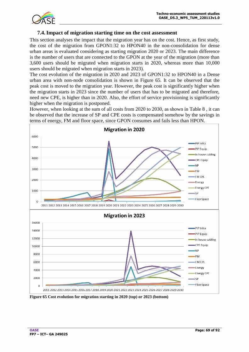
Techno-economic assessment studies OASE_D5.3_WP5_TUM_220113v1.0
OASE FP7 – ICT– GA 249025
Page: 69 of 92
7.4. Impact of migration starting time on the cost assessment
This section analyses the impact that the migration year has on the cost. Hence, as first study,
the cost of the migration from GPON1:32 to HPON40 in the non-consolidation for dense
urban areas is evaluated considering as starting migration 2020 or 2023. The main difference
is the number of users that are connected to the GPON at the year of the migration (more than
3,600 users should be migrated when migration starts in 2020, whereas more than 10,000
users should be migrated when migration starts in 2023).
The cost evolution of the migration in 2020 and 2023 of GPON1:32 to HPON40 in a Dense
urban area with non-node consolidation is shown in Figure 65. It can be observed that the
peak cost is moved to the migration year. However, the peak cost is significantly higher when
the migration starts in 2023 since the number of users that has to be migrated and therefore,
need new CPE, is higher than in 2020. Also, the effort of service provisioning is significantly
higher when the migration is postponed.
However, when looking at the sum of all costs from 2020 to 2030, as shown in Table 8 , it can
be observed that the increase of SP and CPE costs is compensated somehow by the savings in
terms of energy, FM and floor space, since GPON consumes and fails less than HPON.
Figure 65 Cost evolution for migration starting in 2020 (top) or 2023 (bottom)
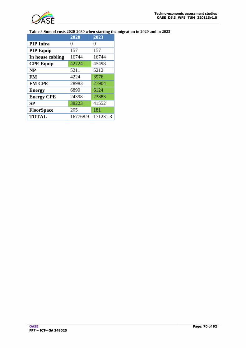
Techno-economic assessment studies OASE_D5.3_WP5_TUM_220113v1.0
OASE FP7 – ICT– GA 249025
Page: 70 of 92
Table 8 Sum of costs 2020-2030 when starting the migration in 2020 and in 2023
2020 2023
PIP Infra 0 0
PIP Equip 157 157
In house cabling 16744 16744
CPE Equip 42724 45498
NP 5211 5212
FM 4224 3976
FM CPE 28983 27904
Energy 6899 6124
Energy CPE 24398 23883
SP 38223 41552
FloorSpace 205 181
TOTAL 167768.9 171231.3
Techno-economic assessment studies OASE_D5.3_WP5_TUM_220113v1.0
OASE FP7 – ICT– GA 249025
Page: 71 of 92
8. Sensitivity analysis
In this deliverable different estimations and predictions have been shown for the total cost of
ownership of an NGOA network. These figures are the results from using the TCO tool
developed within WP5 taking into account the requirements as described in WP2, the
architectures as described in WP3 and the components in WP4. Results from the calculations
in this tool will flow to WP6 for further analysis. Clearly the reliability of the TCO tool
should be investigated and in extension the effect of potential changes in the input parameters
on the outcome total cost of ownership is very important.
In order to test the tool and get a better feeling of its input parameters and the effect on the
outcome a set of sensitivity analysis studies have been performed. In discussion with the other
work packages – in their interest and from their background – the following studies have been
defined:
1. Impact of the requirements from WP2 on the outcome of the total cost of ownership.
The main requirements of OASE have been to provide a sustainable bandwidth of 500
Mbps or higher over a distance of 100km and with a fanout of 1000 customers per
feeder fibre. Clearly loosening one of these requirements will have an impact on the
other. In this study we increased the fanout in order to check the gains by better
multiplexing and equipment with a higher aggregation factor.
2. Impact of regional differences from WP6 on the outcome of the total cost of
ownership. The TCO tool has been constructed with predefined values for several
parameters inherently giving it a country bias. Different sets for these parameters –
e.g. loans, floor space, energy, etc. – have been constructed in cooperation with WP6
and have been calculated for the different architectures in one sensitivity study.
3. Impact of the relation of the CPE price and the OLT price. When looking at the impact
of the installation of an NGOA, typically both the CPE and the OLT will take the
largest part of the costs. This is even more the case when analyzing the business case
and taking discounting into account, as investment costs are coming early in the
project and will weigh more on the discounted outcome. In this study the impact of
changes in the CPE price on the TCO outcome for the HPON 40 and the HPON 80
architecture will be analyzed.
4. Impact of the adoption rate on the total cost of ownership and especially on the non-
discounted and discounted cost per customer subscription year have been taken into
account.
All studies as described in this list have been conducted and the input and outcome results are
discussed in more detail in the following subsections.
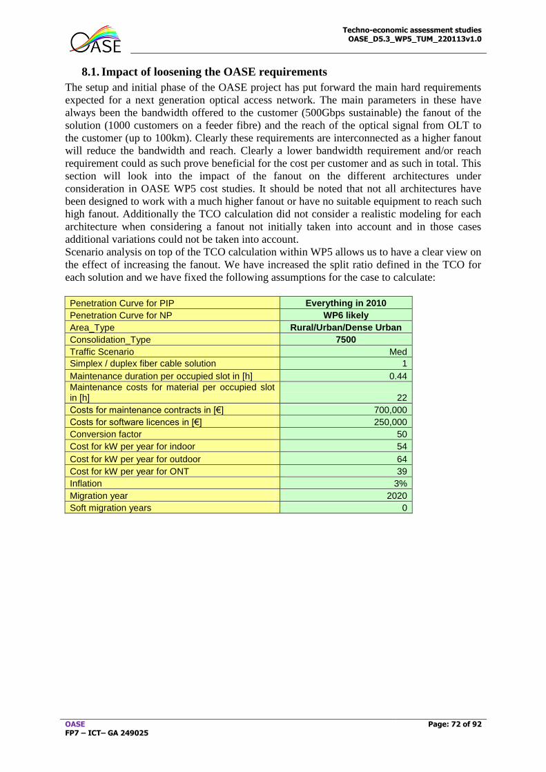
Techno-economic assessment studies OASE_D5.3_WP5_TUM_220113v1.0
OASE FP7 – ICT– GA 249025
Page: 72 of 92
8.1. Impact of loosening the OASE requirements
The setup and initial phase of the OASE project has put forward the main hard requirements
expected for a next generation optical access network. The main parameters in these have
always been the bandwidth offered to the customer (500Gbps sustainable) the fanout of the
solution (1000 customers on a feeder fibre) and the reach of the optical signal from OLT to
the customer (up to 100km). Clearly these requirements are interconnected as a higher fanout
will reduce the bandwidth and reach. Clearly a lower bandwidth requirement and/or reach
requirement could as such prove beneficial for the cost per customer and as such in total. This
section will look into the impact of the fanout on the different architectures under
consideration in OASE WP5 cost studies. It should be noted that not all architectures have
been designed to work with a much higher fanout or have no suitable equipment to reach such
high fanout. Additionally the TCO calculation did not consider a realistic modeling for each
architecture when considering a fanout not initially taken into account and in those cases
additional variations could not be taken into account.
Scenario analysis on top of the TCO calculation within WP5 allows us to have a clear view on
the effect of increasing the fanout. We have increased the split ratio defined in the TCO for
each solution and we have fixed the following assumptions for the case to calculate:
Penetration Curve for PIP Everything in 2010
Penetration Curve for NP WP6 likely
Area_Type Rural/Urban/Dense Urban
Consolidation_Type 7500
Traffic Scenario Med
Simplex / duplex fiber cable solution 1
Maintenance duration per occupied slot in [h] 0.44
Maintenance costs for material per occupied slot in [h] 22
Costs for maintenance contracts in [€] 700,000
Costs for software licences in [€] 250,000
Conversion factor 50
Cost for kW per year for indoor 54
Cost for kW per year for outdoor 64
Cost for kW per year for ONT 39
Inflation 3%
Migration year 2020
Soft migration years 0
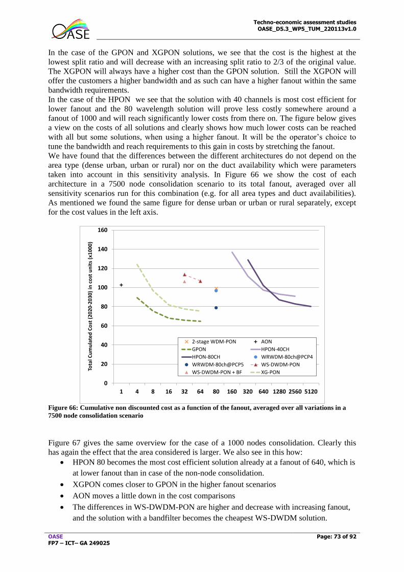
Techno-economic assessment studies OASE_D5.3_WP5_TUM_220113v1.0
OASE FP7 – ICT– GA 249025
Page: 73 of 92
In the case of the GPON and XGPON solutions, we see that the cost is the highest at the
lowest split ratio and will decrease with an increasing split ratio to 2/3 of the original value.
The XGPON will always have a higher cost than the GPON solution. Still the XGPON will
offer the customers a higher bandwidth and as such can have a higher fanout within the same
bandwidth requirements.
In the case of the HPON we see that the solution with 40 channels is most cost efficient for
lower fanout and the 80 wavelength solution will prove less costly somewhere around a
fanout of 1000 and will reach significantly lower costs from there on. The figure below gives
a view on the costs of all solutions and clearly shows how much lower costs can be reached
with all but some solutions, when using a higher fanout. It will be the operator’s choice to
tune the bandwidth and reach requirements to this gain in costs by stretching the fanout.
We have found that the differences between the different architectures do not depend on the
area type (dense urban, urban or rural) nor on the duct availability which were parameters
taken into account in this sensitivity analysis. In Figure 66 we show the cost of each
architecture in a 7500 node consolidation scenario to its total fanout, averaged over all
sensitivity scenarios run for this combination (e.g. for all area types and duct availabilities).
As mentioned we found the same figure for dense urban or urban or rural separately, except
for the cost values in the left axis.
Figure 66: Cumulative non discounted cost as a function of the fanout, averaged over all variations in a
7500 node consolidation scenario
Figure 67 gives the same overview for the case of a 1000 nodes consolidation. Clearly this
has again the effect that the area considered is larger. We also see in this how:
HPON 80 becomes the most cost efficient solution already at a fanout of 640, which is
at lower fanout than in case of the non-node consolidation.
XGPON comes closer to GPON in the higher fanout scenarios
AON moves a little down in the cost comparisons
The differences in WS-DWDM-PON are higher and decrease with increasing fanout,
and the solution with a bandfilter becomes the cheapest WS-DWDM solution.
0
20
40
60
80
100
120
140
160
1 4 8 16 32 64 80 160 320 640 1280 2560 5120
Tota
l Cu
mu
late
d C
ost
(2
02
0-2
03
0)
in c
ost
un
its
(x1
00
0)
2-stage WDM-PON AON
GPON HPON-40CH
HPON-80CH WRWDM-80ch@PCP4
WRWDM-80ch@PCP5 WS-DWDM-PON
WS-DWDM-PON + BF XG-PON
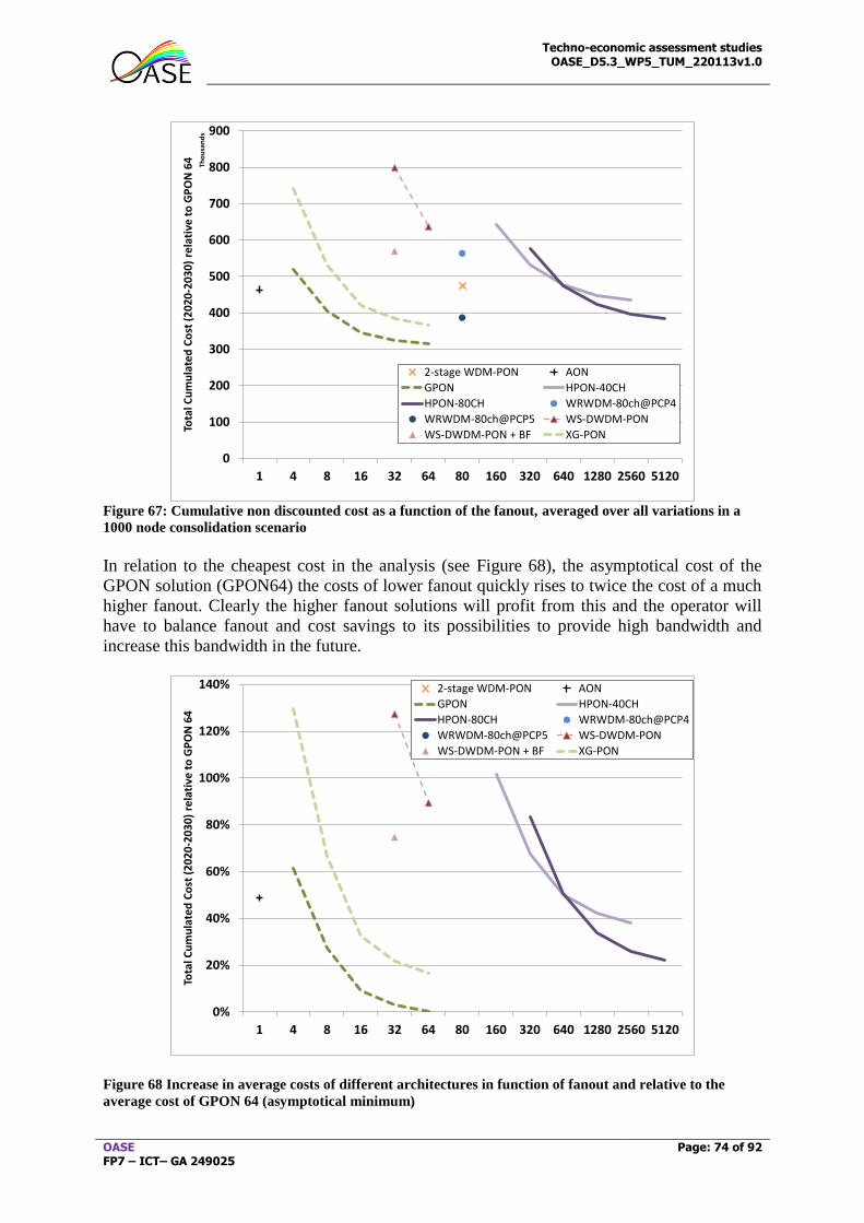
Techno-economic assessment studies OASE_D5.3_WP5_TUM_220113v1.0
OASE FP7 – ICT– GA 249025
Page: 74 of 92
Figure 67: Cumulative non discounted cost as a function of the fanout, averaged over all variations in a
1000 node consolidation scenario
In relation to the cheapest cost in the analysis (see Figure 68), the asymptotical cost of the
GPON solution (GPON64) the costs of lower fanout quickly rises to twice the cost of a much
higher fanout. Clearly the higher fanout solutions will profit from this and the operator will
have to balance fanout and cost savings to its possibilities to provide high bandwidth and
increase this bandwidth in the future.
Figure 68 Increase in average costs of different architectures in function of fanout and relative to the
average cost of GPON 64 (asymptotical minimum)
0
100
200
300
400
500
600
700
800
900
1 4 8 16 32 64 80 160 320 640 1280 2560 5120
Tota
l Cu
mu
late
d C
ost
(2
02
0-2
03
0)
rela
tive
to
GP
ON
64
Th
ou
san
ds
2-stage WDM-PON AON
GPON HPON-40CH
HPON-80CH WRWDM-80ch@PCP4
WRWDM-80ch@PCP5 WS-DWDM-PON
WS-DWDM-PON + BF XG-PON
0%
20%
40%
60%
80%
100%
120%
140%
1 4 8 16 32 64 80 160 320 640 1280 2560 5120
Tota
l Cu
mu
late
d C
ost
(2
02
0-2
03
0)
rela
tive
to
GP
ON
64
2-stage WDM-PON AON
GPON HPON-40CH
HPON-80CH WRWDM-80ch@PCP4
WRWDM-80ch@PCP5 WS-DWDM-PON
WS-DWDM-PON + BF XG-PON
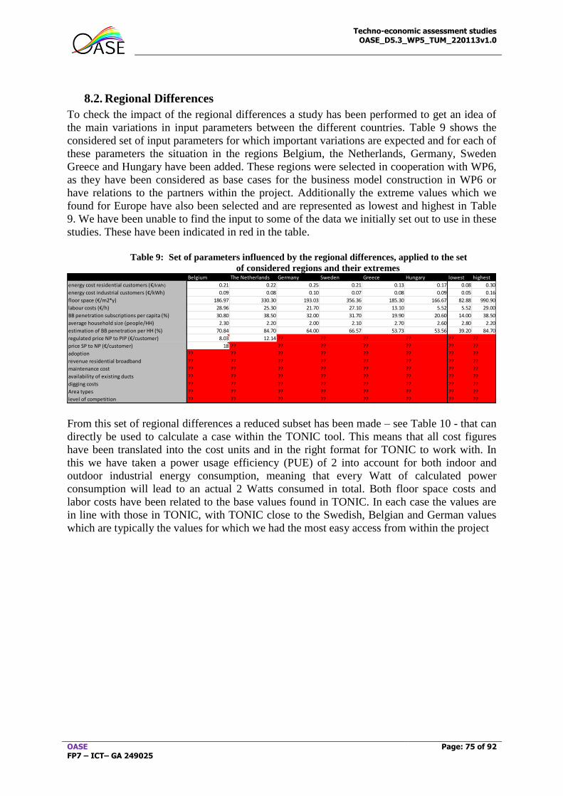
Techno-economic assessment studies OASE_D5.3_WP5_TUM_220113v1.0
OASE FP7 – ICT– GA 249025
Page: 75 of 92
8.2. Regional Differences
To check the impact of the regional differences a study has been performed to get an idea of
the main variations in input parameters between the different countries. Table 9 shows the
considered set of input parameters for which important variations are expected and for each of
these parameters the situation in the regions Belgium, the Netherlands, Germany, Sweden
Greece and Hungary have been added. These regions were selected in cooperation with WP6,
as they have been considered as base cases for the business model construction in WP6 or
have relations to the partners within the project. Additionally the extreme values which we
found for Europe have also been selected and are represented as lowest and highest in Table
9. We have been unable to find the input to some of the data we initially set out to use in these
studies. These have been indicated in red in the table.
Table 9: Set of parameters influenced by the regional differences, applied to the set
of considered regions and their extremes
From this set of regional differences a reduced subset has been made – see Table 10 - that can
directly be used to calculate a case within the TONIC tool. This means that all cost figures
have been translated into the cost units and in the right format for TONIC to work with. In
this we have taken a power usage efficiency (PUE) of 2 into account for both indoor and
outdoor industrial energy consumption, meaning that every Watt of calculated power
consumption will lead to an actual 2 Watts consumed in total. Both floor space costs and
labor costs have been related to the base values found in TONIC. In each case the values are
in line with those in TONIC, with TONIC close to the Swedish, Belgian and German values
which are typically the values for which we had the most easy access from within the project
Belgium The Netherlands Germany Sweden Greece Hungary lowest highest
energy cost residential customers (€/kWh) 0.21 0.22 0.25 0.21 0.13 0.17 0.08 0.30
energy cost industrial customers (€/kWh) 0.09 0.08 0.10 0.07 0.08 0.09 0.05 0.16
floor space (€/m2*y) 186.97 330.30 193.03 356.36 185.30 166.67 82.88 990.90
labour costs (€/h) 28.96 25.30 21.70 27.10 13.10 5.52 5.52 29.00
BB penetration subscriptions per capita (%) 30.80 38.50 32.00 31.70 19.90 20.60 14.00 38.50
average household size (people/HH) 2.30 2.20 2.00 2.10 2.70 2.60 2.80 2.20
estimation of BB penetration per HH (%) 70.84 84.70 64.00 66.57 53.73 53.56 39.20 84.70
regulated price NP to PIP (€/customer) 8.03 12.14 ?? ?? ?? ?? ?? ??
price SP to NP (€/customer) 18 ?? ?? ?? ?? ?? ?? ??
adoption ?? ?? ?? ?? ?? ?? ?? ??
revenue residential broadband ?? ?? ?? ?? ?? ?? ?? ??
maintenance cost ?? ?? ?? ?? ?? ?? ?? ??
availability of existing ducts ?? ?? ?? ?? ?? ?? ?? ??
digging costs ?? ?? ?? ?? ?? ?? ?? ??
Area types ?? ?? ?? ?? ?? ?? ?? ??
level of competition ?? ?? ?? ?? ?? ?? ?? ??
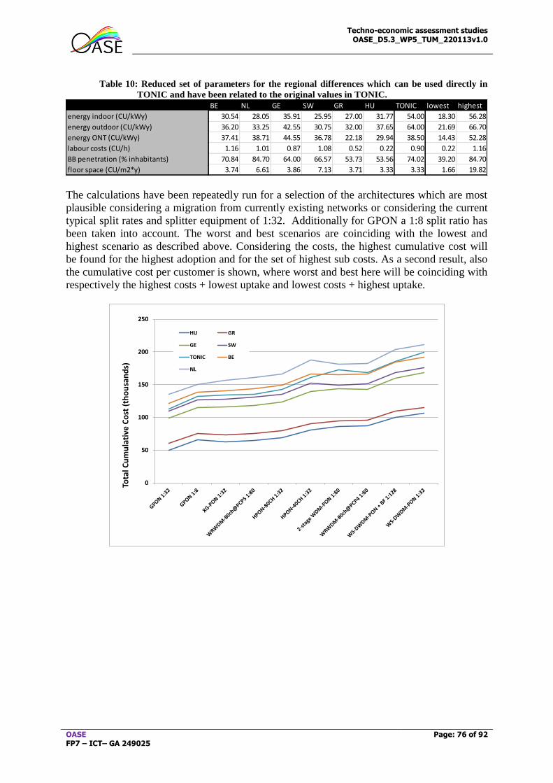
Techno-economic assessment studies OASE_D5.3_WP5_TUM_220113v1.0
OASE FP7 – ICT– GA 249025
Page: 76 of 92
Table 10: Reduced set of parameters for the regional differences which can be used directly in
TONIC and have been related to the original values in TONIC.
The calculations have been repeatedly run for a selection of the architectures which are most
plausible considering a migration from currently existing networks or considering the current
typical split rates and splitter equipment of 1:32. Additionally for GPON a 1:8 split ratio has
been taken into account. The worst and best scenarios are coinciding with the lowest and
highest scenario as described above. Considering the costs, the highest cumulative cost will
be found for the highest adoption and for the set of highest sub costs. As a second result, also
the cumulative cost per customer is shown, where worst and best here will be coinciding with
respectively the highest costs + lowest uptake and lowest costs + highest uptake.
BE NL GE SW GR HU TONIC lowest highest
energy indoor (CU/kWy) 30.54 28.05 35.91 25.95 27.00 31.77 54.00 18.30 56.28
energy outdoor (CU/kWy) 36.20 33.25 42.55 30.75 32.00 37.65 64.00 21.69 66.70
energy ONT (CU/kWy) 37.41 38.71 44.55 36.78 22.18 29.94 38.50 14.43 52.28
labour costs (CU/h) 1.16 1.01 0.87 1.08 0.52 0.22 0.90 0.22 1.16
BB penetration (% inhabitants) 70.84 84.70 64.00 66.57 53.73 53.56 74.02 39.20 84.70
floor space (CU/m2*y) 3.74 6.61 3.86 7.13 3.71 3.33 3.33 1.66 19.82
0
50
100
150
200
250
Tota
l Cu
mu
lati
ve C
ost
(th
ou
san
ds)
HU GR
GE SW
TONIC BE
NL
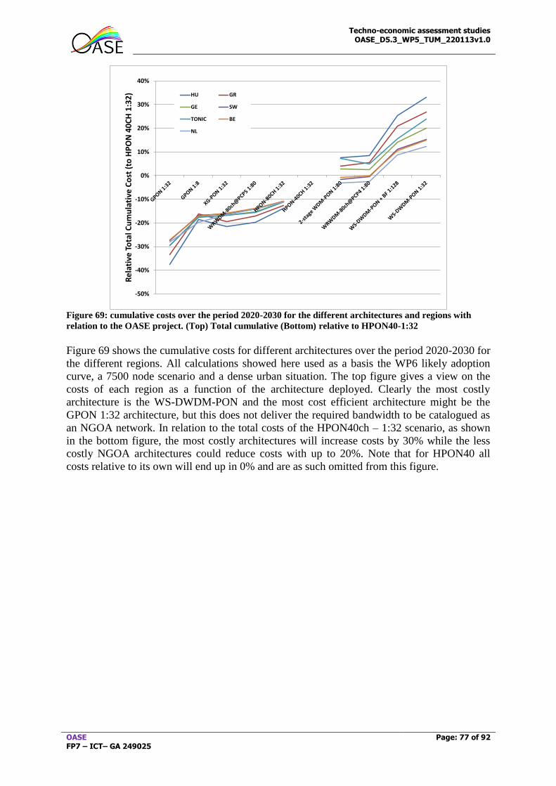
Techno-economic assessment studies OASE_D5.3_WP5_TUM_220113v1.0
OASE FP7 – ICT– GA 249025
Page: 77 of 92
Figure 69: cumulative costs over the period 2020-2030 for the different architectures and regions with
relation to the OASE project. (Top) Total cumulative (Bottom) relative to HPON40-1:32
Figure 69 shows the cumulative costs for different architectures over the period 2020-2030 for
the different regions. All calculations showed here used as a basis the WP6 likely adoption
curve, a 7500 node scenario and a dense urban situation. The top figure gives a view on the
costs of each region as a function of the architecture deployed. Clearly the most costly
architecture is the WS-DWDM-PON and the most cost efficient architecture might be the
GPON 1:32 architecture, but this does not deliver the required bandwidth to be catalogued as
an NGOA network. In relation to the total costs of the HPON40ch – 1:32 scenario, as shown
in the bottom figure, the most costly architectures will increase costs by 30% while the less
costly NGOA architectures could reduce costs with up to 20%. Note that for HPON40 all
costs relative to its own will end up in 0% and are as such omitted from this figure.
-50%
-40%
-30%
-20%
-10%
0%
10%
20%
30%
40%
Re
lati
ve T
ota
l Cu
mu
lati
ve C
ost
(to
HP
ON
40
CH
1:3
2) HU GR
GE SW
TONIC BE
NL
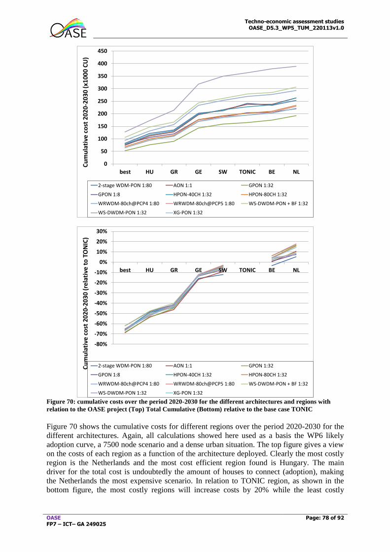
Techno-economic assessment studies OASE_D5.3_WP5_TUM_220113v1.0
OASE FP7 – ICT– GA 249025
Page: 78 of 92
Figure 70: cumulative costs over the period 2020-2030 for the different architectures and regions with
relation to the OASE project (Top) Total Cumulative (Bottom) relative to the base case TONIC
Figure 70 shows the cumulative costs for different regions over the period 2020-2030 for the
different architectures. Again, all calculations showed here used as a basis the WP6 likely
adoption curve, a 7500 node scenario and a dense urban situation. The top figure gives a view
on the costs of each region as a function of the architecture deployed. Clearly the most costly
region is the Netherlands and the most cost efficient region found is Hungary. The main
driver for the total cost is undoubtedly the amount of houses to connect (adoption), making
the Netherlands the most expensive scenario. In relation to TONIC region, as shown in the
bottom figure, the most costly regions will increase costs by 20% while the least costly
0
50
100
150
200
250
300
350
400
450
best HU GR GE SW TONIC BE NL
Cu
mu
lati
ve c
ost
20
20
-20
30
(x1
00
0 C
U)
2-stage WDM-PON 1:80 AON 1:1 GPON 1:32
GPON 1:8 HPON-40CH 1:32 HPON-80CH 1:32
WRWDM-80ch@PCP4 1:80 WRWDM-80ch@PCP5 1:80 WS-DWDM-PON + BF 1:32
WS-DWDM-PON 1:32 XG-PON 1:32
-80%
-70%
-60%
-50%
-40%
-30%
-20%
-10%
0%
10%
20%
30%
best HU GR GE SW TONIC BE NL
Cu
mu
lati
ve c
ost
20
20-
20
30
(re
lati
ve t
o T
ON
IC)
2-stage WDM-PON 1:80 AON 1:1 GPON 1:32
GPON 1:8 HPON-40CH 1:32 HPON-80CH 1:32
WRWDM-80ch@PCP4 1:80 WRWDM-80ch@PCP5 1:80 WS-DWDM-PON + BF 1:32
WS-DWDM-PON 1:32 XG-PON 1:32
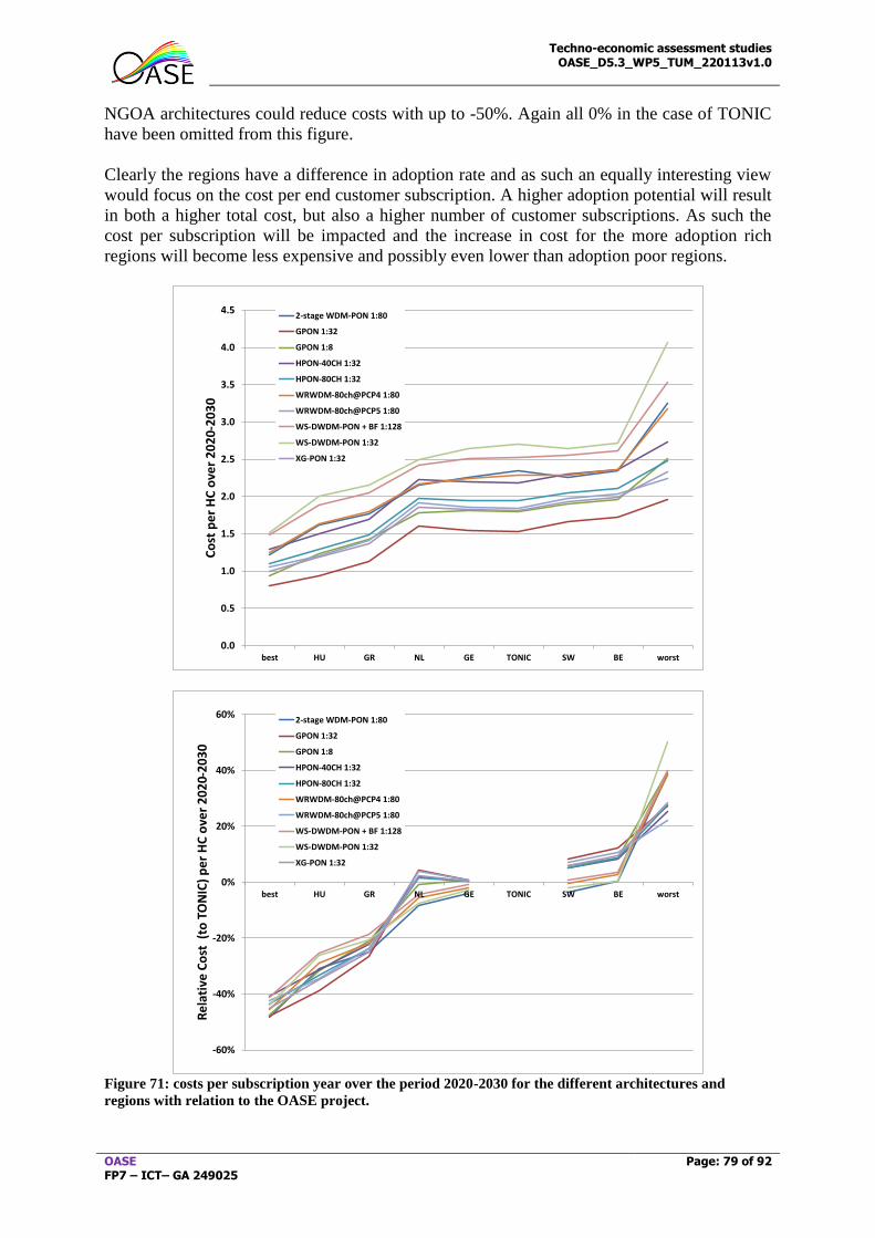
Techno-economic assessment studies OASE_D5.3_WP5_TUM_220113v1.0
OASE FP7 – ICT– GA 249025
Page: 79 of 92
NGOA architectures could reduce costs with up to -50%. Again all 0% in the case of TONIC
have been omitted from this figure.
Clearly the regions have a difference in adoption rate and as such an equally interesting view
would focus on the cost per end customer subscription. A higher adoption potential will result
in both a higher total cost, but also a higher number of customer subscriptions. As such the
cost per subscription will be impacted and the increase in cost for the more adoption rich
regions will become less expensive and possibly even lower than adoption poor regions.
Figure 71: costs per subscription year over the period 2020-2030 for the different architectures and
regions with relation to the OASE project.
0.0
0.5
1.0
1.5
2.0
2.5
3.0
3.5
4.0
4.5
best HU GR NL GE TONIC SW BE worst
Co
st p
er
HC
ove
r 2
02
0-2
03
0
2-stage WDM-PON 1:80
GPON 1:32
GPON 1:8
HPON-40CH 1:32
HPON-80CH 1:32
WRWDM-80ch@PCP4 1:80
WRWDM-80ch@PCP5 1:80
WS-DWDM-PON + BF 1:128
WS-DWDM-PON 1:32
XG-PON 1:32
-60%
-40%
-20%
0%
20%
40%
60%
best HU GR NL GE TONIC SW BE worst
Re
lati
ve C
ost
(to
TO
NIC
) p
er
HC
ove
r 2
02
0-2
03
0
2-stage WDM-PON 1:80
GPON 1:32
GPON 1:8
HPON-40CH 1:32
HPON-80CH 1:32
WRWDM-80ch@PCP4 1:80
WRWDM-80ch@PCP5 1:80
WS-DWDM-PON + BF 1:128
WS-DWDM-PON 1:32
XG-PON 1:32
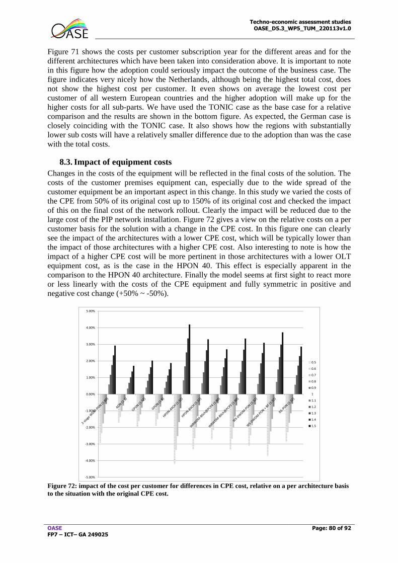
Techno-economic assessment studies OASE_D5.3_WP5_TUM_220113v1.0
OASE FP7 – ICT– GA 249025
Page: 80 of 92
Figure 71 shows the costs per customer subscription year for the different areas and for the
different architectures which have been taken into consideration above. It is important to note
in this figure how the adoption could seriously impact the outcome of the business case. The
figure indicates very nicely how the Netherlands, although being the highest total cost, does
not show the highest cost per customer. It even shows on average the lowest cost per
customer of all western European countries and the higher adoption will make up for the
higher costs for all sub-parts. We have used the TONIC case as the base case for a relative
comparison and the results are shown in the bottom figure. As expected, the German case is
closely coinciding with the TONIC case. It also shows how the regions with substantially
lower sub costs will have a relatively smaller difference due to the adoption than was the case
with the total costs.
8.3. Impact of equipment costs
Changes in the costs of the equipment will be reflected in the final costs of the solution. The
costs of the customer premises equipment can, especially due to the wide spread of the
customer equipment be an important aspect in this change. In this study we varied the costs of
the CPE from 50% of its original cost up to 150% of its original cost and checked the impact
of this on the final cost of the network rollout. Clearly the impact will be reduced due to the
large cost of the PIP network installation. Figure 72 gives a view on the relative costs on a per
customer basis for the solution with a change in the CPE cost. In this figure one can clearly
see the impact of the architectures with a lower CPE cost, which will be typically lower than
the impact of those architectures with a higher CPE cost. Also interesting to note is how the
impact of a higher CPE cost will be more pertinent in those architectures with a lower OLT
equipment cost, as is the case in the HPON 40. This effect is especially apparent in the
comparison to the HPON 40 architecture. Finally the model seems at first sight to react more
or less linearly with the costs of the CPE equipment and fully symmetric in positive and
negative cost change (+50% ~ -50%).
Figure 72: impact of the cost per customer for differences in CPE cost, relative on a per architecture basis
to the situation with the original CPE cost.
-5.00%
-4.00%
-3.00%
-2.00%
-1.00%
0.00%
1.00%
2.00%
3.00%
4.00%
5.00%
0.5
0.6
0.7
0.8
0.9
1
1.1
1.2
1.3
1.4
1.5
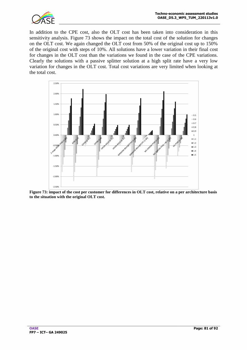
Techno-economic assessment studies OASE_D5.3_WP5_TUM_220113v1.0
OASE FP7 – ICT– GA 249025
Page: 81 of 92
In addition to the CPE cost, also the OLT cost has been taken into consideration in this
sensitivity analysis. Figure 73 shows the impact on the total cost of the solution for changes
on the OLT cost. We again changed the OLT cost from 50% of the original cost up to 150%
of the original cost with steps of 10%. All solutions have a lower variation in their final cost
for changes in the OLT cost than the variations we found in the case of the CPE variations.
Clearly the solutions with a passive splitter solution at a high split rate have a very low
variation for changes in the OLT cost. Total cost variations are very limited when looking at
the total cost.
Figure 73: impact of the cost per customer for differences in OLT cost, relative on a per architecture basis
to the situation with the original OLT cost.
-2.50%
-2.00%
-1.50%
-1.00%
-0.50%
0.00%
0.50%
1.00%
1.50%
2.00%
2.50%
0.5
0.6
0.7
0.8
0.9
1
1.1
1.2
1.3
1.4
1.5
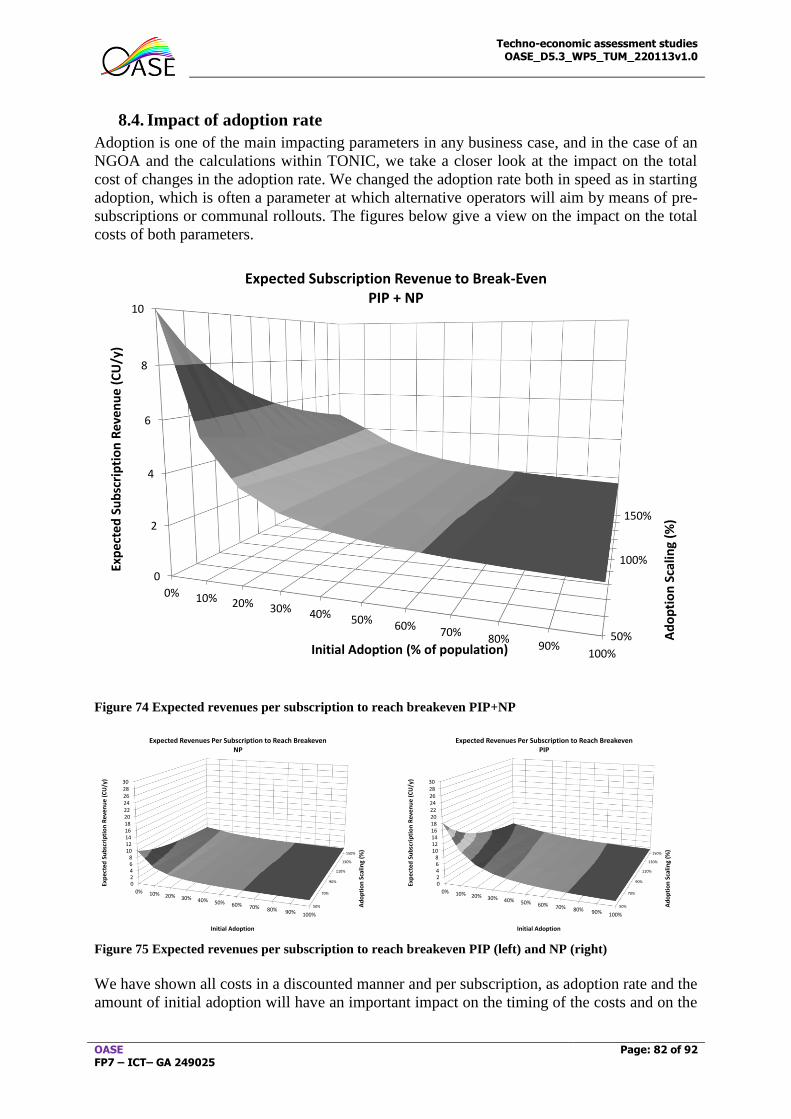
Techno-economic assessment studies OASE_D5.3_WP5_TUM_220113v1.0
OASE FP7 – ICT– GA 249025
Page: 82 of 92
8.4. Impact of adoption rate
Adoption is one of the main impacting parameters in any business case, and in the case of an
NGOA and the calculations within TONIC, we take a closer look at the impact on the total
cost of changes in the adoption rate. We changed the adoption rate both in speed as in starting
adoption, which is often a parameter at which alternative operators will aim by means of pre-
subscriptions or communal rollouts. The figures below give a view on the impact on the total
costs of both parameters.
Figure 74 Expected revenues per subscription to reach breakeven PIP+NP
Figure 75 Expected revenues per subscription to reach breakeven PIP (left) and NP (right)
We have shown all costs in a discounted manner and per subscription, as adoption rate and the
amount of initial adoption will have an important impact on the timing of the costs and on the
50%
100%
150%
0
2
4
6
8
10
0% 10% 20% 30% 40% 50% 60%70%
80%90%
100%
Ad
op
tio
n S
calin
g (%
)
Exp
ect
ed
Su
bsc
rip
tio
n R
eve
nu
e (
CU
/y)
Initial Adoption (% of population)
Expected Subscription Revenue to Break-EvenPIP + NP
50%
70%
90%
110%
130%
150%
02468
1012141618202224262830
0% 10% 20% 30% 40% 50% 60% 70% 80% 90% 100%
Ad
op
tio
n S
calin
g (%
)
Exp
ect
ed
Su
bsc
rip
tio
n R
eve
nu
e (
CU
/y)
Initial Adoption
Expected Revenues Per Subscription to Reach BreakevenNP
50%
70%
90%
110%
130%
150%
02468
1012141618202224262830
0% 10% 20% 30% 40% 50% 60% 70% 80% 90% 100%
Ad
op
tio
n S
calin
g (%
)
Exp
ect
ed
Su
bsc
rip
tio
n R
eve
nu
e (
CU
/y)
Initial Adoption
Expected Revenues Per Subscription to Reach BreakevenPIP
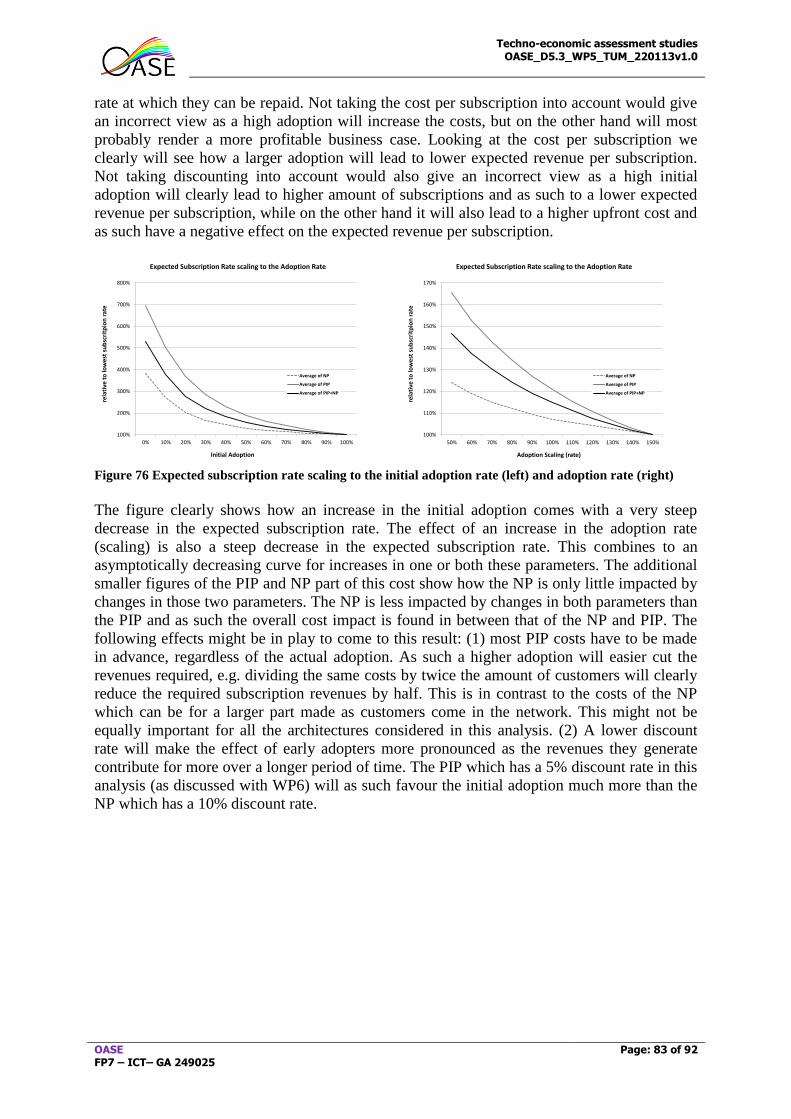
Techno-economic assessment studies OASE_D5.3_WP5_TUM_220113v1.0
OASE FP7 – ICT– GA 249025
Page: 83 of 92
rate at which they can be repaid. Not taking the cost per subscription into account would give
an incorrect view as a high adoption will increase the costs, but on the other hand will most
probably render a more profitable business case. Looking at the cost per subscription we
clearly will see how a larger adoption will lead to lower expected revenue per subscription.
Not taking discounting into account would also give an incorrect view as a high initial
adoption will clearly lead to higher amount of subscriptions and as such to a lower expected
revenue per subscription, while on the other hand it will also lead to a higher upfront cost and
as such have a negative effect on the expected revenue per subscription.
Figure 76 Expected subscription rate scaling to the initial adoption rate (left) and adoption rate (right)
The figure clearly shows how an increase in the initial adoption comes with a very steep
decrease in the expected subscription rate. The effect of an increase in the adoption rate
(scaling) is also a steep decrease in the expected subscription rate. This combines to an
asymptotically decreasing curve for increases in one or both these parameters. The additional
smaller figures of the PIP and NP part of this cost show how the NP is only little impacted by
changes in those two parameters. The NP is less impacted by changes in both parameters than
the PIP and as such the overall cost impact is found in between that of the NP and PIP. The
following effects might be in play to come to this result: (1) most PIP costs have to be made
in advance, regardless of the actual adoption. As such a higher adoption will easier cut the
revenues required, e.g. dividing the same costs by twice the amount of customers will clearly
reduce the required subscription revenues by half. This is in contrast to the costs of the NP
which can be for a larger part made as customers come in the network. This might not be
equally important for all the architectures considered in this analysis. (2) A lower discount
rate will make the effect of early adopters more pronounced as the revenues they generate
contribute for more over a longer period of time. The PIP which has a 5% discount rate in this
analysis (as discussed with WP6) will as such favour the initial adoption much more than the
NP which has a 10% discount rate.
100%
200%
300%
400%
500%
600%
700%
800%
0% 10% 20% 30% 40% 50% 60% 70% 80% 90% 100%
rela
tive
to
low
est
su
bsc
ritp
ion
rat
e
Initial Adoption
Expected Subscription Rate scaling to the Adoption Rate
Average of NP
Average of PIP
Average of PIP+NP
100%
110%
120%
130%
140%
150%
160%
170%
50% 60% 70% 80% 90% 100% 110% 120% 130% 140% 150%
rela
tive
to
low
est
su
bsc
ritp
ion
rat
e
Adoption Scaling (rate)
Expected Subscription Rate scaling to the Adoption Rate
Average of NP
Average of PIP
Average of PIP+NP
Techno-economic assessment studies OASE_D5.3_WP5_TUM_220113v1.0
OASE FP7 – ICT– GA 249025
Page: 84 of 92
9. Conclusion and guidelines
This deliverable presents the cost analysis of different NGOA architectures.
The first cost assessment has been performed considering a migration from an existing
traditional optical access solution (such as GPON or AON) in a non-node consolidation
scenario. The cost assessment shows that the architectures have higher a OPEX than CAPEX
when summing the costs from 2020 to 2030 (NGOA operational time) for any type of area
(i.e. DU, U and R). The most costly architecture is the UDWDM for any area, whereas the
less costly solution is to keep existing optical access networks and upgrade existing GPON by
reducing the splitting ration from 32 to 8 so that the bandwidth increases or to keep the AON
as it is. The CAPEX key cost factors of these architectures differ: for UDWDM is NP and
CPE equipment, for AON is the NP equipment and in-house infrastructure, whereas for the
GPON upgrade is CPE and in-house infrastructure. Regarding OPEX, the most important
factor is the service provisioning. The impact of energy and FM differs significantly on the
architecture (e.g. UDWDM has high energy and FM but relatively low CPE energy cost;
AON has low CPE related costs; whereas GPON has lower values but slightly higher CPE
energy cost).
When considering node consolidation, multiple architectures have been evaluated since they
can offer the long reach requirements while keeping the high bandwidth per user. In this
scenario, it can be observed that the upgrade of GPON by reducing the splitting ratio is not an
option due to the high costs related to the new LL5 links (increases more than 1 CU/year per
user). Some architectures keep and even decrease their average TCO per user per year when
applied to aggressive node consolidation scenarios: e.g. HPON40 (for any area) and
WSWDM PON (for DU) solutions. Furthermore, the options to connect AON AS with a
WDM Backhaul, or migrate from GPON to HPON architecture are the most effective
solutions for any type of area applying node consolidation. It has to be mentioned that extra
savings could be expected on the reduction of cost due to liberation of central offices as well
as on the concentration of A/C and Power systems, which have not been included in the study
due to missing data.
In an NP brownfield scenario, the cost key factors that have been identified are: the SP and
any related CPE parameter such as cost, energy consumption (and failure rate which is related
to the FM that includes the replacement of the CPE).
The migration for most of the studies has been assumed to start in 2020 and last one year,
which is a realistic for one area and cost estimations can be extracted when no discounted
values are considered. However, the impact of the duration of the migration has been
evaluated by comparing the results with a longer migration of 3 years for the particular case
of GPON to HPON migration scenario. The conclusion is that a longer migration process
softens the cost peaks of ONT cost and SP, while having small impact to the other cost
parameters. Furthermore, a later migration impacts significantly the ONT and SP cost since
the later the migration starts, the more users need to be migrated and hence, higher investment
in terms of CPE and SP.
The impact of duct availability (related to the possibility to have a greenfield or more
brownfield PIP) on the infrastructure cost differs on the architecture and on the area: higher
for DU than rural areas, higher for AON P2P and WRWDM PON than HPON solutions.
Finally the sensitivity analysis has rendered us with a more detailed view on what happens
when the main influencing aspects in the context of the network rollout are changed. These
led to the following results:

Techno-economic assessment studies OASE_D5.3_WP5_TUM_220113v1.0
OASE FP7 – ICT– GA 249025
Page: 85 of 92
- A higher fanout will for all architectures lead to a lower cost per home passed and to a
lower overall cost. Cost reductions up to 30% and more are reachable by increasing the
fanout substantially. It should be noted that the higher fanout cases might conflict with the
consolidation possibilities – as a higher fanout will reduce the reach – and maximum
dedicated bandwidth – as with a higher fanout, more customers are sharing the same OLT
port. Relaxing the OASE requirements – for instance only in an initial phase – could as
such reduce the upfront costs substantially
- Regional differences could lead to a very different cost of deployment. Especially in those
European countries with lower average salaries, the costs could be much lower. Next to
the salary, the adoption is the most important impacting factor and a higher adoption will
lead to a lower cost per customer in the end.
- The impact of costs of the ONT and OLT equipment behaves more or less linear for all
architectures and has a rather limited impact up to resp. ~5% or ~2% for an increase up to
50% of its original cost.
- Adoption has most probably the highest impact of all factors and has been split into initial
adoption effect (e.g. by means of presubscriptions) and the steepness of the adoption
curve. Increases in the initial adoption lead to the most substantial decrease in the cost per
subscription year. Still the effect of having a faster adoption is certainly very important.
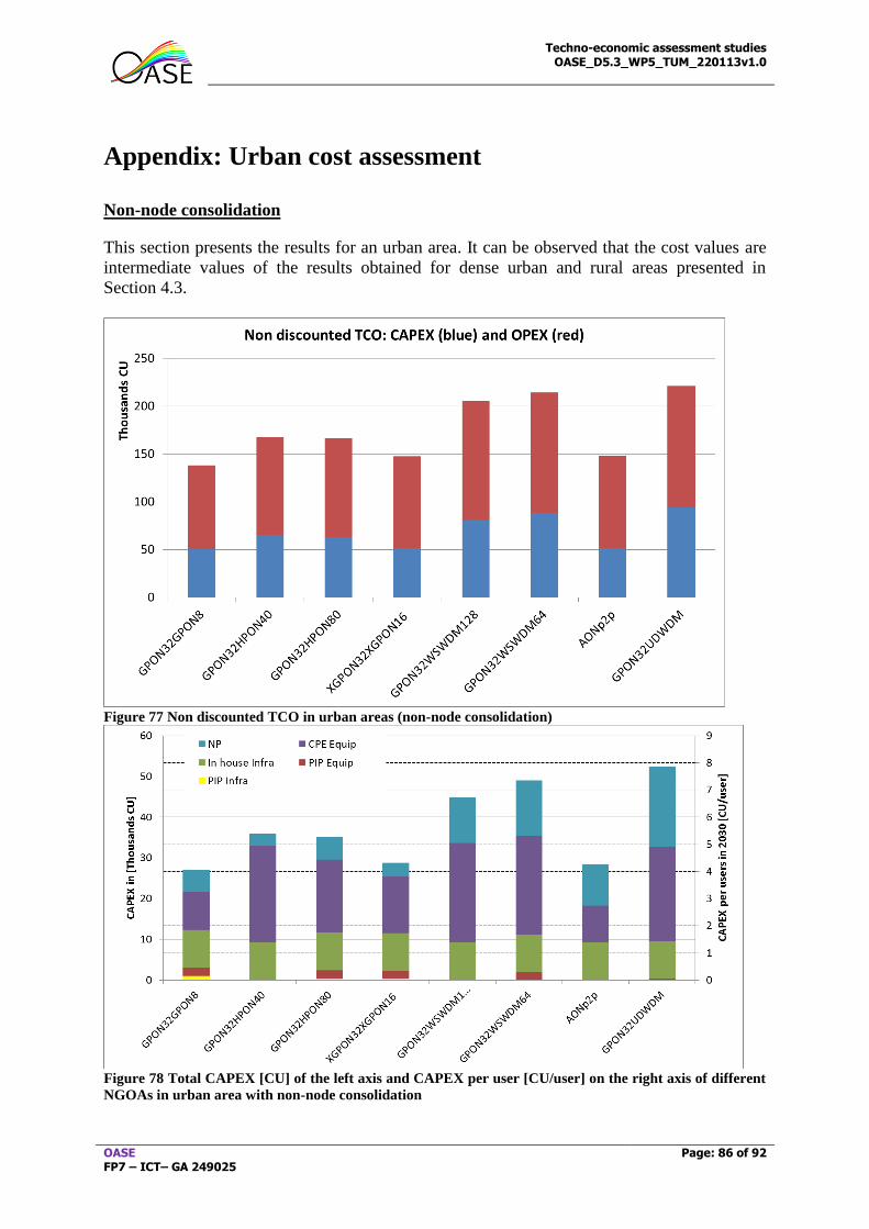
Techno-economic assessment studies OASE_D5.3_WP5_TUM_220113v1.0
OASE FP7 – ICT– GA 249025
Page: 86 of 92
Appendix: Urban cost assessment
Non-node consolidation
This section presents the results for an urban area. It can be observed that the cost values are
intermediate values of the results obtained for dense urban and rural areas presented in
Section 4.3.
Figure 77 Non discounted TCO in urban areas (non-node consolidation)
Figure 78 Total CAPEX [CU] of the left axis and CAPEX per user [CU/user] on the right axis of different
NGOAs in urban area with non-node consolidation
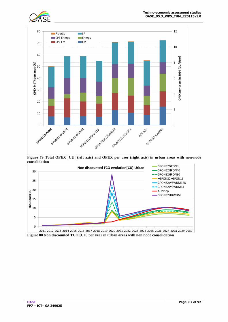
Techno-economic assessment studies OASE_D5.3_WP5_TUM_220113v1.0
OASE FP7 – ICT– GA 249025
Page: 87 of 92
Figure 79 Total OPEX [CU] (left axis) and OPEX per user (right axis) in urban areas with non-node
consolidation
Figure 80 Non discounted TCO [CU] per year in urban areas with non node consolidation
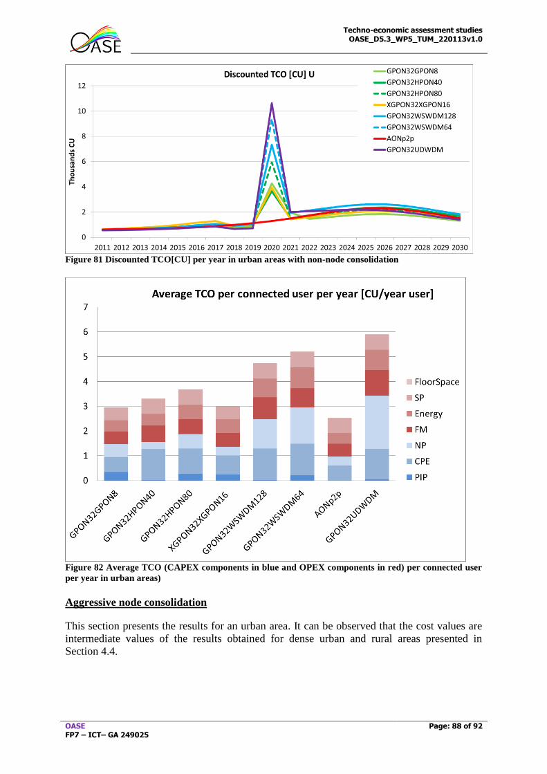
Techno-economic assessment studies OASE_D5.3_WP5_TUM_220113v1.0
OASE FP7 – ICT– GA 249025
Page: 88 of 92
Figure 81 Discounted TCO[CU] per year in urban areas with non-node consolidation
Figure 82 Average TCO (CAPEX components in blue and OPEX components in red) per connected user
per year in urban areas)
Aggressive node consolidation
This section presents the results for an urban area. It can be observed that the cost values are
intermediate values of the results obtained for dense urban and rural areas presented in
Section 4.4.
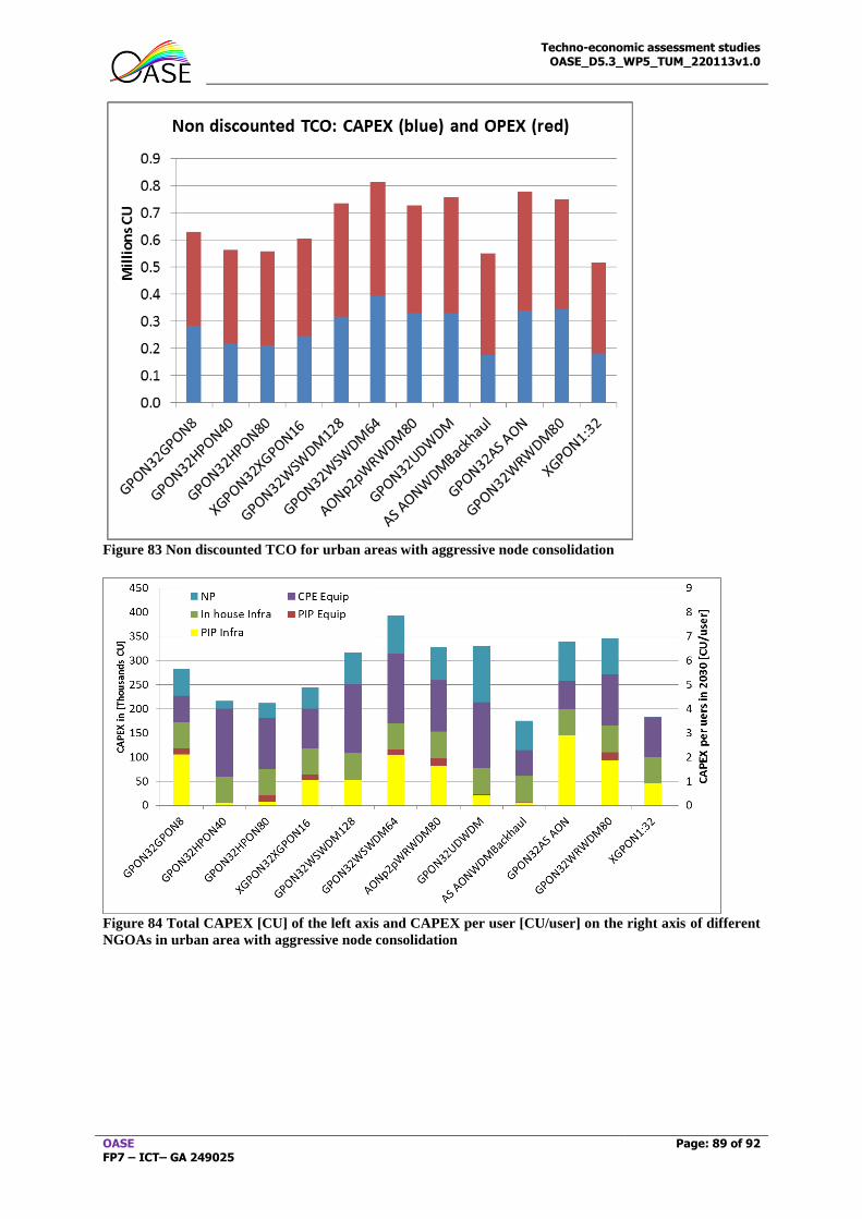
Techno-economic assessment studies OASE_D5.3_WP5_TUM_220113v1.0
OASE FP7 – ICT– GA 249025
Page: 89 of 92
Figure 83 Non discounted TCO for urban areas with aggressive node consolidation
Figure 84 Total CAPEX [CU] of the left axis and CAPEX per user [CU/user] on the right axis of different
NGOAs in urban area with aggressive node consolidation
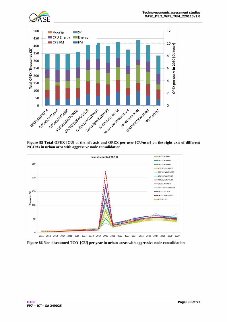
Techno-economic assessment studies OASE_D5.3_WP5_TUM_220113v1.0
OASE FP7 – ICT– GA 249025
Page: 90 of 92
Figure 85 Total OPEX [CU] of the left axis and OPEX per user [CU/user] on the right axis of different
NGOAs in urban area with aggressive node consolidation
Figure 86 Non discounted TCO [CU] per year in urban areas with aggressive node consolidation
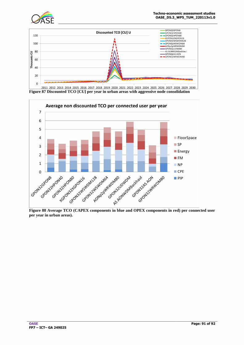
Techno-economic assessment studies OASE_D5.3_WP5_TUM_220113v1.0
OASE FP7 – ICT– GA 249025
Page: 91 of 92
Figure 87 Discounted TCO [CU] per year in urban areas with aggressive node consolidation
Figure 88 Average TCO (CAPEX components in blue and OPEX components in red) per connected user
per year in urban areas).

Techno-economic assessment studies OASE_D5.3_WP5_TUM_220113v1.0
OASE FP7 – ICT– GA 249025
Page: 92 of 92
Appendix B: Assumptions of cost assessment
This section summarizes some assumptions considered in the cost assessment:
Fault Management
As presented in D5.2, the fault management process consists of three main parts: pre-
processing of the failure, failure reparation and post-processing of the reparation. The fault
management process is triggered by the number of expected failures of any of the network
components (either equipment or infrastructure), which is given as FIT rate.
The pre-processing includes the detection, help desk, opening TT, etc. and has been assumed
to the same for all failures.
The reparation of the failure depends on the network component that has failed. Each network
component has associated an average reparation time (MTTR), a travelling time to the failure
location and the number of required technicians. The only exceptions are the ONTs since in
these cases, no technician is associated to the ONT reparation, but rather a new ONT is
shipped to the user.
The post processing of the reparation, which includes any required test and the TT closing is
also assumed to the same for all failures.
Aggressive node consolidation
When applying the network dimensioning to the aggressive node consolidation, the required
LL5 is computed considering that 50% of the trenching and duct is required. The number of
LL5 fibres is calculated based on the number of PCP5s that have to be connected to the new
OLT location (PCP6). However, these LL5 fibres are grouped into different ducts based on
the aggregation factor of each case (i.e. how many traditional access areas are grouped into
one new consolidated area).