Embed Size (px)
Citation preview
NWChem User Documentation
Release 4.0.1
High Performance Computational Chemistry GroupW.R. Wiley Environmental Molecular Sciences Laboratory
Pacific Northwest National LaboratoryP.O. Box 999, Richland, WA 99352
January 2001

2

DISCLAIMER
This material was prepared as an account of work sponsored by an agency of the United States Government. Neitherthe United States Government nor the United States Department of Energy, nor Battelle, nor any of their employees,MAKES ANY WARRANTY, EXPRESS OR IMPLIED, OR ASSUMES ANY LEGAL LIABILITY OR RESPON-SIBILITY FOR THE ACCURACY, COMPLETENESS, OR USEFULNESS OF ANY INFORMATION, APPARA-TUS, PRODUCT, SOFTWARE, OR PROCESS DISCLOSED, OR REPRESENTS THAT ITS USE WOULD NOTINFRINGE PRIVATELY OWNED RIGHTS.
LIMITED USE
This software (including any documentation) is being made available to you for your internal use only, solely foruse in performance of work directly for the U.S. Federal Government or work under contracts with the U.S. Departmentof Energy or other U.S. Federal Government agencies. This software is a version which has not yet been evaluated andcleared for commercialization. Adherence to this notice may be necessary for the author, Battelle Memorial Institute,to successfully assert copyright in and commercialize this software. This software is not intended for duplication ordistribution to third parties without the permission of the Manager of Software Products at Pacific Northwest NationalLaboratory, Richland, Washington, 99352.
ACKNOWLEDGMENT
This software and its documentation were produced with Government support under Contract Number DE-AC06-76RLO-1830 awarded by the United States Department of Energy. The Government retains a paid-up non-exclusive,irrevocable worldwide license to reproduce, prepare derivative works, perform publicly and display publicly by or forthe Government, including the right to distribute to other Government contractors.
3

4
AUTHOR DISCLAIMER
This software contains proprietary information of the authors, Pacific Northwest National Laboratory (PNNL),and the US Department of Energy (USDOE). The information herein shall not be disclosed to others, and shall not bereproduced whole or in part, without written permission from PNNL or USDOE. The information contained in thisdocument is provided “AS IS” without guarantee of accuracy. Use of this software is prohibited withoutwritten per-mission from PNNL or USDOE. The authors, PNNL, and USDOE make no representations or warranties whatsoeverwith respect to this software, including the implied warranty of merchant-ability or fitness for a particular purpose.The user assumes all risks, including consequential loss or damage, in respect to the use of the software. In addition,PNNL and the authors shall not be obligated to correct or maintain the program, or notify the user community ofmodifications or updates that will be made over the course of time.
Contents
1 Introduction 17
1.1 Citation . . . . . . . . . . . . . . . . . . . . . . . . . . . . . . . . . . . . . . . . . . . . . . . . . . 17
1.2 User Feedback . . . . . . . . . . . . . . . . . . . . . . . . . . . . . . . . . . . . . . . . . . . . . . 18
2 Getting Started 19
2.1 Input File Structure . . . . . . . . . . . . . . . . . . . . . . . . . . . . . . . . . . . . . . . . . . . . 19
2.2 Simple Input File — SCF geometry optimization . . . . . . . . . . . . . . . . . . . . . . . . . . . . 20
2.3 Water Molecule Sample Input File . . . . . . . . . . . . . . . . . . . . . . . . . . . . . . . . . . . . 21
2.4 Input Format and Syntax for Directives . . . . . . . . . . . . . . . . . . . . . . . . . . . . . . . . . . 23
2.4.1 Input Format . . . . . . . . . . . . . . . . . . . . . . . . . . . . . . . . . . . . . . . . . . . 23
2.4.2 Format and syntax of directives . . . . . . . . . . . . . . . . . . . . . . . . . . . . . . . . . 24
3 NWChem Architecture 27
3.1 Database Structure . . . . . . . . . . . . . . . . . . . . . . . . . . . . . . . . . . . . . . . . . . . . 27
3.2 Persistence of data and restart . . . . . . . . . . . . . . . . . . . . . . . . . . . . . . . . . . . . . . . 29
4 Functionality 31
4.1 Molecular electronic structure . . . . . . . . . . . . . . . . . . . . . . . . . . . . . . . . . . . . . . 31
4.2 Relativistic effects . . . . . . . . . . . . . . . . . . . . . . . . . . . . . . . . . . . . . . . . . . . . . 32
4.3 Pseudopotential plane-wave electronic structure . . . . . . . . . . . . . . . . . . . . . . . . . . . . . 33
4.4 Periodic system electronic structure . . . . . . . . . . . . . . . . . . . . . . . . . . . . . . . . . . . 33
4.5 Molecular dynamics . . . . . . . . . . . . . . . . . . . . . . . . . . . . . . . . . . . . . . . . . . . . 33
4.6 Python . . . . . . . . . . . . . . . . . . . . . . . . . . . . . . . . . . . . . . . . . . . . . . . . . . . 34
4.7 Parallel tools and libraries (ParSoft) . . . . . . . . . . . . . . . . . . . . . . . . . . . . . . . . . . . 34
5 Top-level directives 35
5.1 START and RESTART — Start-up mode . . . . . . . . . . . . . . . . . . . . . . . . . . . . . . . . . 35
5
6 CONTENTS
5.2 SCRATCH_DIR and PERMANENT_DIR — File directories . . . . . . . . . . . . . . . . . . . . . . 36
5.3 MEMORY — Control of memory limits . . . . . . . . . . . . . . . . . . . . . . . . . . . . . . . . . 38
5.4 ECHO — Print input file . . . . . . . . . . . . . . . . . . . . . . . . . . . . . . . . . . . . . . . . . 39
5.5 TITLE — Specify job title . . . . . . . . . . . . . . . . . . . . . . . . . . . . . . . . . . . . . . . . 40
5.6 PRINT and NOPRINT — Print control . . . . . . . . . . . . . . . . . . . . . . . . . . . . . . . . . . 40
5.7 SET — Enter data in the RTDB . . . . . . . . . . . . . . . . . . . . . . . . . . . . . . . . . . . . . 41
5.8 UNSET — Delete data in the RTDB . . . . . . . . . . . . . . . . . . . . . . . . . . . . . . . . . . . 43
5.9 STOP — Terminate processing . . . . . . . . . . . . . . . . . . . . . . . . . . . . . . . . . . . . . . 43
5.10 TASK — Perform a task . . . . . . . . . . . . . . . . . . . . . . . . . . . . . . . . . . . . . . . . . 44
5.10.1 TASK Directive for Electronic Structure Calculations . . . . . . . . . . . . . . . . . . . . . . 44
5.10.2 TASK Directive for Special Operations . . . . . . . . . . . . . . . . . . . . . . . . . . . . . 45
5.10.3 TASK Directive for the Bourne Shell . . . . . . . . . . . . . . . . . . . . . . . . . . . . . . 46
5.10.4 TASK Directive for QM/MM simulations . . . . . . . . . . . . . . . . . . . . . . . . . . . . 47
5.11 CHARGE — Total system charge . . . . . . . . . . . . . . . . . . . . . . . . . . . . . . . . . . . . 47
6 Geometries 49
6.1 Keywords on the GEOMETRY directive . . . . . . . . . . . . . . . . . . . . . . . . . . . . . . . . . 50
6.2 Symmetry Group Input . . . . . . . . . . . . . . . . . . . . . . . . . . . . . . . . . . . . . . . . . . 52
6.3 Cartesian coordinate input . . . . . . . . . . . . . . . . . . . . . . . . . . . . . . . . . . . . . . . . 53
6.4 Z-matrix input . . . . . . . . . . . . . . . . . . . . . . . . . . . . . . . . . . . . . . . . . . . . . . . 54
6.5 ZCOORD — Forcing internal coordinates . . . . . . . . . . . . . . . . . . . . . . . . . . . . . . . . 59
6.6 Applying constraints in geometry optimizations . . . . . . . . . . . . . . . . . . . . . . . . . . . . . 60
6.7 SYSTEM — Lattice parameters for periodic systems . . . . . . . . . . . . . . . . . . . . . . . . . . 61
7 Basis sets 63
7.1 Basis set library . . . . . . . . . . . . . . . . . . . . . . . . . . . . . . . . . . . . . . . . . . . . . . 64
7.2 Explicit basis set definition . . . . . . . . . . . . . . . . . . . . . . . . . . . . . . . . . . . . . . . . 65
8 Effective Core Potentials 67
8.1 Scalar ECPs . . . . . . . . . . . . . . . . . . . . . . . . . . . . . . . . . . . . . . . . . . . . . . . . 68
8.2 Spin-orbit ECPs . . . . . . . . . . . . . . . . . . . . . . . . . . . . . . . . . . . . . . . . . . . . . . 70
9 Relativistic All-electron Approximations 71
9.1 Douglas-Kroll approximation . . . . . . . . . . . . . . . . . . . . . . . . . . . . . . . . . . . . . . . 72
9.2 Dyall’s Modified Dirac Hamitonian approximation . . . . . . . . . . . . . . . . . . . . . . . . . . . 72
CONTENTS 7
10 Hartree-Fock or Self-consistent Field 77
10.1 Wavefunction type . . . . . . . . . . . . . . . . . . . . . . . . . . . . . . . . . . . . . . . . . . . . 77
10.2 SYM — use of symmetry . . . . . . . . . . . . . . . . . . . . . . . . . . . . . . . . . . . . . . . . . 78
10.3 ADAPT – symmetry adaptation of MOs . . . . . . . . . . . . . . . . . . . . . . . . . . . . . . . . . 78
10.4 TOL2E — integral screening threshold . . . . . . . . . . . . . . . . . . . . . . . . . . . . . . . . . . 79
10.5 VECTORS — input/output of MO vectors . . . . . . . . . . . . . . . . . . . . . . . . . . . . . . . . 79
10.5.1 Superposition of fragment molecular orbitals . . . . . . . . . . . . . . . . . . . . . . . . . . 81
10.5.2 Atomic guess orbitals with charged atoms . . . . . . . . . . . . . . . . . . . . . . . . . . . . 86
10.6 Accuracy of initial guess . . . . . . . . . . . . . . . . . . . . . . . . . . . . . . . . . . . . . . . . . 87
10.7 THRESH — convergence threshold . . . . . . . . . . . . . . . . . . . . . . . . . . . . . . . . . . . 87
10.8 MAXITER — iteration limit . . . . . . . . . . . . . . . . . . . . . . . . . . . . . . . . . . . . . . . 88
10.9 RI-SCF — resolution of the identity approximation . . . . . . . . . . . . . . . . . . . . . . . . . . . 88
10.10PROFILE — performance profile . . . . . . . . . . . . . . . . . . . . . . . . . . . . . . . . . . . . . 89
10.11DIIS — DIIS convergence . . . . . . . . . . . . . . . . . . . . . . . . . . . . . . . . . . . . . . . . 89
10.12DIRECT and SEMIDIRECT — recomputation of integrals . . . . . . . . . . . . . . . . . . . . . . . 90
10.12.1 Integral File Size and Format for the SCF Module . . . . . . . . . . . . . . . . . . . . . . . . 91
10.13SCF Convergence Control Options . . . . . . . . . . . . . . . . . . . . . . . . . . . . . . . . . . . . 92
10.14NR — controlling the Newton-Raphson . . . . . . . . . . . . . . . . . . . . . . . . . . . . . . . . . 93
10.15LEVEL — level-shifting the orbital Hessian . . . . . . . . . . . . . . . . . . . . . . . . . . . . . . . 93
10.16Orbtial Localization . . . . . . . . . . . . . . . . . . . . . . . . . . . . . . . . . . . . . . . . . . . . 94
10.17Printing Information from the SCF Module . . . . . . . . . . . . . . . . . . . . . . . . . . . . . . . 96
10.18Hartree-Fock or SCF, MCSCF and MP2 Gradients . . . . . . . . . . . . . . . . . . . . . . . . . . . 97
11 DFT for Molecules (DFT) 99
11.1 Specification of Basis Sets for the DFT Module . . . . . . . . . . . . . . . . . . . . . . . . . . . . . 101
11.2 VECTORS and MAX_OVL — KS-MO Vectors . . . . . . . . . . . . . . . . . . . . . . . . . . . . . 102
11.3 XC and DECOMP — Exchange-Correlation Potentials . . . . . . . . . . . . . . . . . . . . . . . . . 102
11.3.1 Optional Exchange Functionals . . . . . . . . . . . . . . . . . . . . . . . . . . . . . . . . . 103
11.3.2 Optional Correlation Functionals . . . . . . . . . . . . . . . . . . . . . . . . . . . . . . . . . 104
11.3.3 Combined Exchange and Correlation Functionals . . . . . . . . . . . . . . . . . . . . . . . . 105
11.4 ITERATIONS — Number of SCF iterations . . . . . . . . . . . . . . . . . . . . . . . . . . . . . . . 108
11.5 CONVERGENCE — SCF Convergence Control . . . . . . . . . . . . . . . . . . . . . . . . . . . . 108
11.6 GRID — Numerical Integration of the XC Potential . . . . . . . . . . . . . . . . . . . . . . . . . . . 110
11.6.1 Angular grids . . . . . . . . . . . . . . . . . . . . . . . . . . . . . . . . . . . . . . . . . . . 113
11.6.2 Partitioning functions . . . . . . . . . . . . . . . . . . . . . . . . . . . . . . . . . . . . . . . 115
8 CONTENTS
11.6.3 Radial grids . . . . . . . . . . . . . . . . . . . . . . . . . . . . . . . . . . . . . . . . . . . . 115
11.6.4 Grid Scheme . . . . . . . . . . . . . . . . . . . . . . . . . . . . . . . . . . . . . . . . . . . 115
11.7 TOLERANCES — Screening tolerances . . . . . . . . . . . . . . . . . . . . . . . . . . . . . . . . . 116
11.8 DIRECT and NOIO — Hardware Resource Control . . . . . . . . . . . . . . . . . . . . . . . . . . . 116
11.9 DFT, ODFT and MULT — Open shell systems . . . . . . . . . . . . . . . . . . . . . . . . . . . . . 117
11.10SIC — Self-Interaction Correction . . . . . . . . . . . . . . . . . . . . . . . . . . . . . . . . . . . . 117
11.11MULLIKEN — Mulliken analysis . . . . . . . . . . . . . . . . . . . . . . . . . . . . . . . . . . . . 118
11.12Print Control . . . . . . . . . . . . . . . . . . . . . . . . . . . . . . . . . . . . . . . . . . . . . . . 118
12 Spin-Orbit DFT (SODFT) 119
13 COSMO 123
14 DFT for Periodic Systems (GAPSS) 127
14.1 Specification of Basis Sets for the GAPSS Module . . . . . . . . . . . . . . . . . . . . . . . . . . . 128
14.2 CORRELATIONandEXCHANGE— Exchange-Correlation Potentials . . . . . . . . . . . . . . . . . 128
14.2.1 Optional Functionals . . . . . . . . . . . . . . . . . . . . . . . . . . . . . . . . . . . . . . . 129
14.3 Numerical Integration . . . . . . . . . . . . . . . . . . . . . . . . . . . . . . . . . . . . . . . . . . . 130
14.4 Summations and Integrations for a Periodic System . . . . . . . . . . . . . . . . . . . . . . . . . . . 130
14.5 SCF Iterative Procedure . . . . . . . . . . . . . . . . . . . . . . . . . . . . . . . . . . . . . . . . . . 130
15 MP2 133
15.1 Input directives . . . . . . . . . . . . . . . . . . . . . . . . . . . . . . . . . . . . . . . . . . . . . . 133
15.1.1 FREEZE— Freezing orbitals . . . . . . . . . . . . . . . . . . . . . . . . . . . . . . . . . . 134
15.1.2 TIGHT — Increased precision . . . . . . . . . . . . . . . . . . . . . . . . . . . . . . . . . . 135
15.1.3 PRINT andNOPRINT . . . . . . . . . . . . . . . . . . . . . . . . . . . . . . . . . . . . . . 135
15.1.4 VECTORS— MO vectors . . . . . . . . . . . . . . . . . . . . . . . . . . . . . . . . . . . . 135
15.1.5 RI-MP2 fitting basis . . . . . . . . . . . . . . . . . . . . . . . . . . . . . . . . . . . . . . . 136
15.1.6 FILE3C — RI-MP2 3-center integral filename . . . . . . . . . . . . . . . . . . . . . . . . . 136
15.1.7 RIAPPROX— RI-MP2 Approximation . . . . . . . . . . . . . . . . . . . . . . . . . . . . . 137
15.1.8 Advanced options for RI-MP2 . . . . . . . . . . . . . . . . . . . . . . . . . . . . . . . . . . 137
15.2 One-electron properties and natural orbitals . . . . . . . . . . . . . . . . . . . . . . . . . . . . . . . 139
16 Multiconfiguration SCF 141
16.1 ACTIVE — Number of active orbitals . . . . . . . . . . . . . . . . . . . . . . . . . . . . . . . . . . 141
16.2 ACTELEC— Number of active electrons . . . . . . . . . . . . . . . . . . . . . . . . . . . . . . . . 142
CONTENTS 9
16.3 MULTIPLICITY . . . . . . . . . . . . . . . . . . . . . . . . . . . . . . . . . . . . . . . . . . . . . 142
16.4 SYMMETRY— Spatial symmetry of the wavefunction . . . . . . . . . . . . . . . . . . . . . . . . . . 142
16.5 STATE— Symmetry and multiplicity . . . . . . . . . . . . . . . . . . . . . . . . . . . . . . . . . . 142
16.6 VECTORS— Input/output of MO vectors . . . . . . . . . . . . . . . . . . . . . . . . . . . . . . . . 143
16.7 HESSIAN— Select preconditioner . . . . . . . . . . . . . . . . . . . . . . . . . . . . . . . . . . . 143
16.8 LEVEL— Level shift for convergence . . . . . . . . . . . . . . . . . . . . . . . . . . . . . . . . . . 143
16.9 PRINT andNOPRINT . . . . . . . . . . . . . . . . . . . . . . . . . . . . . . . . . . . . . . . . . . 143
17 Selected CI 145
17.1 Background . . . . . . . . . . . . . . . . . . . . . . . . . . . . . . . . . . . . . . . . . . . . . . . . 145
17.2 Files . . . . . . . . . . . . . . . . . . . . . . . . . . . . . . . . . . . . . . . . . . . . . . . . . . . . 146
17.3 Configuration Generation . . . . . . . . . . . . . . . . . . . . . . . . . . . . . . . . . . . . . . . . . 147
17.3.1 Specifying the reference occupation . . . . . . . . . . . . . . . . . . . . . . . . . . . . . . . 147
17.3.2 Applying creation-annihilation operators . . . . . . . . . . . . . . . . . . . . . . . . . . . . 148
17.3.3 Uniform excitation level . . . . . . . . . . . . . . . . . . . . . . . . . . . . . . . . . . . . . 149
17.4 Number of roots . . . . . . . . . . . . . . . . . . . . . . . . . . . . . . . . . . . . . . . . . . . . . . 149
17.5 Accuracy of diagonalization . . . . . . . . . . . . . . . . . . . . . . . . . . . . . . . . . . . . . . . 149
17.6 Selection thresholds . . . . . . . . . . . . . . . . . . . . . . . . . . . . . . . . . . . . . . . . . . . . 150
17.7 Mode . . . . . . . . . . . . . . . . . . . . . . . . . . . . . . . . . . . . . . . . . . . . . . . . . . . 150
17.8 Memory requirements . . . . . . . . . . . . . . . . . . . . . . . . . . . . . . . . . . . . . . . . . . . 150
17.9 Forcing regeneration of the MO integrals . . . . . . . . . . . . . . . . . . . . . . . . . . . . . . . . . 150
17.10Disabling update of the configuration list . . . . . . . . . . . . . . . . . . . . . . . . . . . . . . . . . 150
17.11Orbital locking in ci geometry optimization . . . . . . . . . . . . . . . . . . . . . . . . . . . . . . . 151
18 Coupled Cluster Calculations 153
18.1 MAXITER— Maximum number of iterations . . . . . . . . . . . . . . . . . . . . . . . . . . . . . . 153
18.2 THRESH— Convergence threshold . . . . . . . . . . . . . . . . . . . . . . . . . . . . . . . . . . . 154
18.3 TOL2E— integral screening threshold . . . . . . . . . . . . . . . . . . . . . . . . . . . . . . . . . . 154
18.4 DIISBAS — DIIS subspace dimension . . . . . . . . . . . . . . . . . . . . . . . . . . . . . . . . . 154
18.5 FREEZE— Freezing orbitals . . . . . . . . . . . . . . . . . . . . . . . . . . . . . . . . . . . . . . . 154
18.6 IPRT — Debug printing . . . . . . . . . . . . . . . . . . . . . . . . . . . . . . . . . . . . . . . . . 154
18.7 PRINT and NOPRINT . . . . . . . . . . . . . . . . . . . . . . . . . . . . . . . . . . . . . . . . . . 155
18.8 Methods (Tasks) Recognized . . . . . . . . . . . . . . . . . . . . . . . . . . . . . . . . . . . . . . . 155
18.9 Debugging and Development Aids . . . . . . . . . . . . . . . . . . . . . . . . . . . . . . . . . . . . 155
18.9.1 Switching On and Off Terms . . . . . . . . . . . . . . . . . . . . . . . . . . . . . . . . . . . 155
10 CONTENTS
19 Geometry Optimization with DRIVER 157
19.1 Convergence criteria . . . . . . . . . . . . . . . . . . . . . . . . . . . . . . . . . . . . . . . . . . . 158
19.2 Available precision . . . . . . . . . . . . . . . . . . . . . . . . . . . . . . . . . . . . . . . . . . . . 158
19.3 Controlling the step length . . . . . . . . . . . . . . . . . . . . . . . . . . . . . . . . . . . . . . . . 158
19.4 Maximum number of steps . . . . . . . . . . . . . . . . . . . . . . . . . . . . . . . . . . . . . . . . 159
19.5 Discard restart information . . . . . . . . . . . . . . . . . . . . . . . . . . . . . . . . . . . . . . . . 159
19.6 Regenerate internal coordinates . . . . . . . . . . . . . . . . . . . . . . . . . . . . . . . . . . . . . . 159
19.7 Initial Hessian . . . . . . . . . . . . . . . . . . . . . . . . . . . . . . . . . . . . . . . . . . . . . . . 159
19.8 Mode or variable to follow to saddle point . . . . . . . . . . . . . . . . . . . . . . . . . . . . . . . . 160
19.9 Optimization history as XYZ files . . . . . . . . . . . . . . . . . . . . . . . . . . . . . . . . . . . . 160
19.10Print options . . . . . . . . . . . . . . . . . . . . . . . . . . . . . . . . . . . . . . . . . . . . . . . . 161
20 Geometry Optimization with STEPPER 163
20.1 MIN andTS — Minimum or transition state search . . . . . . . . . . . . . . . . . . . . . . . . . . . 163
20.2 TRACK— Mode selection . . . . . . . . . . . . . . . . . . . . . . . . . . . . . . . . . . . . . . . . 164
20.3 MAXITER— Maximum number of steps . . . . . . . . . . . . . . . . . . . . . . . . . . . . . . . . 164
20.4 TRUST— Trust radius . . . . . . . . . . . . . . . . . . . . . . . . . . . . . . . . . . . . . . . . . . 164
20.5 CONVGGM, CONVGGandCONVGE— Convergence criteria . . . . . . . . . . . . . . . . . . . . . . . 164
20.6 Backstepping in Stepper . . . . . . . . . . . . . . . . . . . . . . . . . . . . . . . . . . . . . . . . . 165
20.7 Initial Nuclear Hessian Options . . . . . . . . . . . . . . . . . . . . . . . . . . . . . . . . . . . . . . 165
21 Hybrid Calculations with ONIOM 167
21.1 Real, model and intermediate geometries . . . . . . . . . . . . . . . . . . . . . . . . . . . . . . . . . 168
21.1.1 Link atoms . . . . . . . . . . . . . . . . . . . . . . . . . . . . . . . . . . . . . . . . . . . . 169
21.1.2 Numbering of the link atoms . . . . . . . . . . . . . . . . . . . . . . . . . . . . . . . . . . . 170
21.2 High, medium and low theories . . . . . . . . . . . . . . . . . . . . . . . . . . . . . . . . . . . . . . 170
21.2.1 Basis specification . . . . . . . . . . . . . . . . . . . . . . . . . . . . . . . . . . . . . . . . 170
21.2.2 Effective core potentials . . . . . . . . . . . . . . . . . . . . . . . . . . . . . . . . . . . . . 170
21.2.3 General input strings . . . . . . . . . . . . . . . . . . . . . . . . . . . . . . . . . . . . . . . 170
21.3 Use of symmetry . . . . . . . . . . . . . . . . . . . . . . . . . . . . . . . . . . . . . . . . . . . . . 171
21.4 Molecular orbital files . . . . . . . . . . . . . . . . . . . . . . . . . . . . . . . . . . . . . . . . . . . 171
21.5 Restarting . . . . . . . . . . . . . . . . . . . . . . . . . . . . . . . . . . . . . . . . . . . . . . . . . 172
21.6 Examples . . . . . . . . . . . . . . . . . . . . . . . . . . . . . . . . . . . . . . . . . . . . . . . . . 172
21.6.1 Hydrocarbon bond energy . . . . . . . . . . . . . . . . . . . . . . . . . . . . . . . . . . . . 172
21.6.2 Optimization and frequencies . . . . . . . . . . . . . . . . . . . . . . . . . . . . . . . . . . 173
CONTENTS 11
21.6.3 A three-layer example . . . . . . . . . . . . . . . . . . . . . . . . . . . . . . . . . . . . . . 175
21.6.4 DFT with and without charge fitting . . . . . . . . . . . . . . . . . . . . . . . . . . . . . . . 176
22 Vibrational frequencies 179
22.1 Vibrational Module Input . . . . . . . . . . . . . . . . . . . . . . . . . . . . . . . . . . . . . . . . . 179
22.1.1 Hessian File Reuse . . . . . . . . . . . . . . . . . . . . . . . . . . . . . . . . . . . . . . . . 180
22.1.2 Redefining Masses of Elements . . . . . . . . . . . . . . . . . . . . . . . . . . . . . . . . . 180
22.1.3 Animation . . . . . . . . . . . . . . . . . . . . . . . . . . . . . . . . . . . . . . . . . . . . 181
22.1.4 An Example Input Deck . . . . . . . . . . . . . . . . . . . . . . . . . . . . . . . . . . . . . 182
23 DPLOT 183
23.1 GAUSSIAN — Gaussian Cube format . . . . . . . . . . . . . . . . . . . . . . . . . . . . . . . . . . 183
23.2 TITLE — Title for Insight . . . . . . . . . . . . . . . . . . . . . . . . . . . . . . . . . . . . . . . . 183
23.3 LIMITXYZ — Plot limits . . . . . . . . . . . . . . . . . . . . . . . . . . . . . . . . . . . . . . . . 183
23.4 SPIN — Density to be plotted . . . . . . . . . . . . . . . . . . . . . . . . . . . . . . . . . . . . . . 184
23.5 OUTPUT — Filename forInsight . . . . . . . . . . . . . . . . . . . . . . . . . . . . . . . . . . . . 184
23.6 VECTORS — MO vector file name . . . . . . . . . . . . . . . . . . . . . . . . . . . . . . . . . . . 184
23.7 WHERE — Density evaluation . . . . . . . . . . . . . . . . . . . . . . . . . . . . . . . . . . . . . . 184
23.8 ORBITAL — Orbital sub-space . . . . . . . . . . . . . . . . . . . . . . . . . . . . . . . . . . . . . 184
23.9 Examples . . . . . . . . . . . . . . . . . . . . . . . . . . . . . . . . . . . . . . . . . . . . . . . . . 185
24 Properties 187
24.1 Subdirectives . . . . . . . . . . . . . . . . . . . . . . . . . . . . . . . . . . . . . . . . . . . . . . . 188
24.1.1 Nbofile . . . . . . . . . . . . . . . . . . . . . . . . . . . . . . . . . . . . . . . . . . . . . . 188
25 Electrostatic potentials 189
25.1 Grid specification . . . . . . . . . . . . . . . . . . . . . . . . . . . . . . . . . . . . . . . . . . . . . 189
25.2 Constraints . . . . . . . . . . . . . . . . . . . . . . . . . . . . . . . . . . . . . . . . . . . . . . . . 190
25.3 Restraints . . . . . . . . . . . . . . . . . . . . . . . . . . . . . . . . . . . . . . . . . . . . . . . . . 191
26 Prepare 193
26.1 Default database directories . . . . . . . . . . . . . . . . . . . . . . . . . . . . . . . . . . . . . . . . 194
26.2 System name and coordinate source . . . . . . . . . . . . . . . . . . . . . . . . . . . . . . . . . . . 195
26.3 Sequence file generation . . . . . . . . . . . . . . . . . . . . . . . . . . . . . . . . . . . . . . . . . 196
26.4 Topology file generation . . . . . . . . . . . . . . . . . . . . . . . . . . . . . . . . . . . . . . . . . 197
26.5 Appending to an existing topology file . . . . . . . . . . . . . . . . . . . . . . . . . . . . . . . . . . 198
12 CONTENTS
26.6 Generating a restart file . . . . . . . . . . . . . . . . . . . . . . . . . . . . . . . . . . . . . . . . . . 199
27 Molecular dynamics 203
27.1 Introduction . . . . . . . . . . . . . . . . . . . . . . . . . . . . . . . . . . . . . . . . . . . . . . . . 203
27.1.1 Spacial decomposition . . . . . . . . . . . . . . . . . . . . . . . . . . . . . . . . . . . . . . 203
27.1.2 Topology . . . . . . . . . . . . . . . . . . . . . . . . . . . . . . . . . . . . . . . . . . . . . 204
27.1.3 Files . . . . . . . . . . . . . . . . . . . . . . . . . . . . . . . . . . . . . . . . . . . . . . . . 204
27.1.4 Databases . . . . . . . . . . . . . . . . . . . . . . . . . . . . . . . . . . . . . . . . . . . . . 205
27.1.5 Force fields . . . . . . . . . . . . . . . . . . . . . . . . . . . . . . . . . . . . . . . . . . . . 206
27.2 Format of fragment files . . . . . . . . . . . . . . . . . . . . . . . . . . . . . . . . . . . . . . . . . 206
27.3 Creating segment files . . . . . . . . . . . . . . . . . . . . . . . . . . . . . . . . . . . . . . . . . . . 206
27.4 Creating sequence files . . . . . . . . . . . . . . . . . . . . . . . . . . . . . . . . . . . . . . . . . . 206
27.5 Creating topology files . . . . . . . . . . . . . . . . . . . . . . . . . . . . . . . . . . . . . . . . . . 206
27.6 Creating restart files . . . . . . . . . . . . . . . . . . . . . . . . . . . . . . . . . . . . . . . . . . . . 207
27.7 Molecular simulations . . . . . . . . . . . . . . . . . . . . . . . . . . . . . . . . . . . . . . . . . . 207
27.8 System specification . . . . . . . . . . . . . . . . . . . . . . . . . . . . . . . . . . . . . . . . . . . 207
27.9 Parameter set . . . . . . . . . . . . . . . . . . . . . . . . . . . . . . . . . . . . . . . . . . . . . . . 207
27.10Energy minimization algorithms . . . . . . . . . . . . . . . . . . . . . . . . . . . . . . . . . . . . . 208
27.11Multi-configuration thermodynamic integration . . . . . . . . . . . . . . . . . . . . . . . . . . . . . 208
27.12Time and integration algorithm directives . . . . . . . . . . . . . . . . . . . . . . . . . . . . . . . . 209
27.13Ensemble selection . . . . . . . . . . . . . . . . . . . . . . . . . . . . . . . . . . . . . . . . . . . . 210
27.14Velocity reassignments . . . . . . . . . . . . . . . . . . . . . . . . . . . . . . . . . . . . . . . . . . 210
27.15Cutoff radii . . . . . . . . . . . . . . . . . . . . . . . . . . . . . . . . . . . . . . . . . . . . . . . . 210
27.16Polarization . . . . . . . . . . . . . . . . . . . . . . . . . . . . . . . . . . . . . . . . . . . . . . . . 211
27.17External electrostatic field . . . . . . . . . . . . . . . . . . . . . . . . . . . . . . . . . . . . . . . . 211
27.18Constraints . . . . . . . . . . . . . . . . . . . . . . . . . . . . . . . . . . . . . . . . . . . . . . . . 211
27.19Long range interaction corrections . . . . . . . . . . . . . . . . . . . . . . . . . . . . . . . . . . . . 211
27.20Fixing coordinates . . . . . . . . . . . . . . . . . . . . . . . . . . . . . . . . . . . . . . . . . . . . 212
27.21Autocorrelation function . . . . . . . . . . . . . . . . . . . . . . . . . . . . . . . . . . . . . . . . . 212
27.22Print options . . . . . . . . . . . . . . . . . . . . . . . . . . . . . . . . . . . . . . . . . . . . . . . . 212
27.23Periodic updates . . . . . . . . . . . . . . . . . . . . . . . . . . . . . . . . . . . . . . . . . . . . . . 213
27.24Recording . . . . . . . . . . . . . . . . . . . . . . . . . . . . . . . . . . . . . . . . . . . . . . . . . 214
27.25Program control options . . . . . . . . . . . . . . . . . . . . . . . . . . . . . . . . . . . . . . . . . 215
28 Analysis 217
CONTENTS 13
28.1 Reference coordinates . . . . . . . . . . . . . . . . . . . . . . . . . . . . . . . . . . . . . . . . . . . 217
28.2 File specification . . . . . . . . . . . . . . . . . . . . . . . . . . . . . . . . . . . . . . . . . . . . . 217
28.3 Selection . . . . . . . . . . . . . . . . . . . . . . . . . . . . . . . . . . . . . . . . . . . . . . . . . 218
28.4 Coordinate analysis . . . . . . . . . . . . . . . . . . . . . . . . . . . . . . . . . . . . . . . . . . . . 219
28.5 Essential dynamics analysis . . . . . . . . . . . . . . . . . . . . . . . . . . . . . . . . . . . . . . . . 220
28.6 Trajectory format conversion . . . . . . . . . . . . . . . . . . . . . . . . . . . . . . . . . . . . . . . 221
28.7 Electrostatic potentials . . . . . . . . . . . . . . . . . . . . . . . . . . . . . . . . . . . . . . . . . . 222
29 Combined quantum and molecular mechanics 223
29.1 EATOMS . . . . . . . . . . . . . . . . . . . . . . . . . . . . . . . . . . . . . . . . . . . . . . . . . 224
30 File formats 225
31 Pseudopotential Plane-Wave DFT (PSPW) 235
31.1 PSPW Tasks . . . . . . . . . . . . . . . . . . . . . . . . . . . . . . . . . . . . . . . . . . . . . . . . 235
31.1.1 STEEPEST_DESCENT . . . . . . . . . . . . . . . . . . . . . . . . . . . . . . . . . . . . . 236
31.1.2 CONJUGATE_GRADIENT . . . . . . . . . . . . . . . . . . . . . . . . . . . . . . . . . . . 238
31.1.3 Car-Parrinello . . . . . . . . . . . . . . . . . . . . . . . . . . . . . . . . . . . . . . . . . . . 240
31.1.4 PSP_FORMATTER . . . . . . . . . . . . . . . . . . . . . . . . . . . . . . . . . . . . . . . 242
31.1.5 WAVEFUNCTION_INTITIALIZER . . . . . . . . . . . . . . . . . . . . . . . . . . . . . . 243
31.1.6 V_WAVEFUNCTION_INITIALIZER . . . . . . . . . . . . . . . . . . . . . . . . . . . . . . 245
31.1.7 WAVEFUNCTION_EXPANDER . . . . . . . . . . . . . . . . . . . . . . . . . . . . . . . . 246
31.1.8 PSP_GENERATOR . . . . . . . . . . . . . . . . . . . . . . . . . . . . . . . . . . . . . . . 246
31.2 PSPW RTDB Entries and DataFiles . . . . . . . . . . . . . . . . . . . . . . . . . . . . . . . . . . . 249
31.2.1 Ion Positions . . . . . . . . . . . . . . . . . . . . . . . . . . . . . . . . . . . . . . . . . . . 249
31.2.2 Ion Velocities . . . . . . . . . . . . . . . . . . . . . . . . . . . . . . . . . . . . . . . . . . . 249
31.2.3 Simulation Cell . . . . . . . . . . . . . . . . . . . . . . . . . . . . . . . . . . . . . . . . . . 250
31.2.4 Analysis: Mulliken RTDB data . . . . . . . . . . . . . . . . . . . . . . . . . . . . . . . . . 250
31.2.5 Wavefunction Datafile . . . . . . . . . . . . . . . . . . . . . . . . . . . . . . . . . . . . . . 251
31.2.6 Velocity Wavefunction Datafile . . . . . . . . . . . . . . . . . . . . . . . . . . . . . . . . . 251
31.2.7 Formatted Pseudopotential Datafile . . . . . . . . . . . . . . . . . . . . . . . . . . . . . . . 251
31.2.8 One-Dimensional Pseudopotential Datafile . . . . . . . . . . . . . . . . . . . . . . . . . . . 251
31.2.9 PSPW Car-Parrinello Output Datafiles . . . . . . . . . . . . . . . . . . . . . . . . . . . . . . 252
31.3 Minimizing the DFT Energy Functional . . . . . . . . . . . . . . . . . . . . . . . . . . . . . . . . . 253
31.3.1 Steepest Descent Equations . . . . . . . . . . . . . . . . . . . . . . . . . . . . . . . . . . . 253
14 CONTENTS
31.3.2 Conjugate Gradient with Curvature: Grassmann Manifold . . . . . . . . . . . . . . . . . . . 255
31.4 Car-Parrinello Scheme for Ab Initio Molecular Dynamics . . . . . . . . . . . . . . . . . . . . . . . . 257
31.4.1 Verlet Algorithm for Integration . . . . . . . . . . . . . . . . . . . . . . . . . . . . . . . . . 258
31.4.2 Constant Temperature Simulations: Nose-Hoover Thermostats . . . . . . . . . . . . . . . . . 259
31.5 PSPW Tutorial 1: Minimizing the one-electron orbitals by Running a Steepest Descent and ConjuagateGradient Simulation in Tandem . . . . . . . . . . . . . . . . . . . . . . . . . . . . . . . . . . . . . . 260
31.6 PSPW Tutorial 2: Running a Car-Parrinello Simulation . . . . . . . . . . . . . . . . . . . . . . . . . 262
31.7 PSPW Capabilities and Limitations . . . . . . . . . . . . . . . . . . . . . . . . . . . . . . . . . . . . 263
31.8 Questions and Difficulties . . . . . . . . . . . . . . . . . . . . . . . . . . . . . . . . . . . . . . . . . 263
32 Controlling NWChem with Python 265
32.1 How to input and run a Python program inside NWChem . . . . . . . . . . . . . . . . . . . . . . . . 265
32.2 NWChem extensions . . . . . . . . . . . . . . . . . . . . . . . . . . . . . . . . . . . . . . . . . . . 266
32.3 Examples . . . . . . . . . . . . . . . . . . . . . . . . . . . . . . . . . . . . . . . . . . . . . . . . . 267
32.3.1 Hello world . . . . . . . . . . . . . . . . . . . . . . . . . . . . . . . . . . . . . . . . . . . . 267
32.3.2 Scanning a basis exponent . . . . . . . . . . . . . . . . . . . . . . . . . . . . . . . . . . . . 267
32.3.3 Scanning a basis exponent revisited. . . . . . . . . . . . . . . . . . . . . . . . . . . . . . . . 268
32.3.4 Scanning a geometric variable . . . . . . . . . . . . . . . . . . . . . . . . . . . . . . . . . . 269
32.3.5 Scan using the BSSE counterpoise corrected energy . . . . . . . . . . . . . . . . . . . . . . 269
32.3.6 Scan the geometry and compute the energy and gradient . . . . . . . . . . . . . . . . . . . . 270
32.3.7 Reaction energies varying the basis set . . . . . . . . . . . . . . . . . . . . . . . . . . . . . . 271
32.3.8 Using the database . . . . . . . . . . . . . . . . . . . . . . . . . . . . . . . . . . . . . . . . 272
32.3.9 Handling exceptions from NWChem . . . . . . . . . . . . . . . . . . . . . . . . . . . . . . . 272
32.3.10 Accessing geometry information — a temporary hack . . . . . . . . . . . . . . . . . . . . . 273
32.3.11 Scaning a basis exponent yet again — plotting and handling child processes . . . . . . . . . . 274
32.4 Troubleshooting . . . . . . . . . . . . . . . . . . . . . . . . . . . . . . . . . . . . . . . . . . . . . . 275
33 Interfaces to Other Programs 277
33.1 NBO — Natural Bond Orbital Analysis . . . . . . . . . . . . . . . . . . . . . . . . . . . . . . . . . 277
34 Acknowledgments 279
A Standard Basis Sets 281
B Sample input files 295
B.1 Water SCF calculation and geometry optimization in a 6-31g basis . . . . . . . . . . . . . . . . . . . 295
B.1.1 Job 1. Single point SCF energy . . . . . . . . . . . . . . . . . . . . . . . . . . . . . . . . . 295
CONTENTS 15
B.1.2 Job 2. Restarting and perform a geometry optimization . . . . . . . . . . . . . . . . . . . . . 295
B.2 Compute the polarizability of Ne using finite field . . . . . . . . . . . . . . . . . . . . . . . . . . . . 296
B.2.1 Job 1. Compute the atomic energy . . . . . . . . . . . . . . . . . . . . . . . . . . . . . . . . 296
B.2.2 Job 2. Compute the energy with applied field . . . . . . . . . . . . . . . . . . . . . . . . . . 296
B.3 SCF energy of H2CO using ECPs for C and O . . . . . . . . . . . . . . . . . . . . . . . . . . . . . . 296
B.4 MP2 optimization and CCSD(T) on nitrogen . . . . . . . . . . . . . . . . . . . . . . . . . . . . . . . 298
C Examples of geometries using symmetry 301
C.1 Cs methanol . . . . . . . . . . . . . . . . . . . . . . . . . . . . . . . . . . . . . . . . . . . . . . . . 301
C.2 C2v water . . . . . . . . . . . . . . . . . . . . . . . . . . . . . . . . . . . . . . . . . . . . . . . . . 301
C.3 D2h acetylene . . . . . . . . . . . . . . . . . . . . . . . . . . . . . . . . . . . . . . . . . . . . . . . 301
C.4 D2h ethylene . . . . . . . . . . . . . . . . . . . . . . . . . . . . . . . . . . . . . . . . . . . . . . . . 302
C.5 Td methane . . . . . . . . . . . . . . . . . . . . . . . . . . . . . . . . . . . . . . . . . . . . . . . . 302
C.6 Ih buckminsterfullerene . . . . . . . . . . . . . . . . . . . . . . . . . . . . . . . . . . . . . . . . . . 302
C.7 S4 porphyrin . . . . . . . . . . . . . . . . . . . . . . . . . . . . . . . . . . . . . . . . . . . . . . . . 302
C.8 D3h iron penta-carbonyl . . . . . . . . . . . . . . . . . . . . . . . . . . . . . . . . . . . . . . . . . . 303
C.9 D3d sodium crown ether . . . . . . . . . . . . . . . . . . . . . . . . . . . . . . . . . . . . . . . . . 303
C.10C3v ammonia . . . . . . . . . . . . . . . . . . . . . . . . . . . . . . . . . . . . . . . . . . . . . . . 304
C.11 D6h benzene . . . . . . . . . . . . . . . . . . . . . . . . . . . . . . . . . . . . . . . . . . . . . . . . 304
C.12C3h BO3H3 . . . . . . . . . . . . . . . . . . . . . . . . . . . . . . . . . . . . . . . . . . . . . . . . 304
C.13 D5d ferrocene . . . . . . . . . . . . . . . . . . . . . . . . . . . . . . . . . . . . . . . . . . . . . . . 305
C.14C4v SF5Cl . . . . . . . . . . . . . . . . . . . . . . . . . . . . . . . . . . . . . . . . . . . . . . . . . 305
C.15C2h trans-dichloroethylene . . . . . . . . . . . . . . . . . . . . . . . . . . . . . . . . . . . . . . . . 305
C.16 D2d CH2CCH2 . . . . . . . . . . . . . . . . . . . . . . . . . . . . . . . . . . . . . . . . . . . . . . 305
C.17 D5h cyclopentadiene anion . . . . . . . . . . . . . . . . . . . . . . . . . . . . . . . . . . . . . . . . 306
C.18 D4h gold tetrachloride . . . . . . . . . . . . . . . . . . . . . . . . . . . . . . . . . . . . . . . . . . . 306
D Running NWChem 307
D.1 Sequential execution . . . . . . . . . . . . . . . . . . . . . . . . . . . . . . . . . . . . . . . . . . . 307
D.2 Parallel execution on UNIX-based parallel machines including workstation clusters using TCGMSG . 307
D.3 Parallel execution on UNIX-based parallel machines including workstation clusters using MPI . . . . 308
D.4 Parallel execution on MPPs . . . . . . . . . . . . . . . . . . . . . . . . . . . . . . . . . . . . . . . . 309
D.5 IBM SP . . . . . . . . . . . . . . . . . . . . . . . . . . . . . . . . . . . . . . . . . . . . . . . . . . 309
D.6 Cray T3E . . . . . . . . . . . . . . . . . . . . . . . . . . . . . . . . . . . . . . . . . . . . . . . . . 310
D.7 Linux . . . . . . . . . . . . . . . . . . . . . . . . . . . . . . . . . . . . . . . . . . . . . . . . . . . 310

16 CONTENTS
D.8 Alpha systems with Quadrics switch . . . . . . . . . . . . . . . . . . . . . . . . . . . . . . . . . . . 310
D.9 Windows 98 and NT . . . . . . . . . . . . . . . . . . . . . . . . . . . . . . . . . . . . . . . . . . . 311
D.10 Tested Platforms and O/S versions . . . . . . . . . . . . . . . . . . . . . . . . . . . . . . . . . . . . 311
Chapter 1
Introduction
NWChem is a computational chemistry package designed to run on high-performance parallel supercomputers. Codecapabilities include the calculation of molecular electronic energies and analytic gradients using Hartree-Fock self-consistent field (SCF) theory, Gaussian density function theory (DFT), and second-order perturbation theory. For allmethods, geometry optimization is available to determine energy minima and transition states. Classical moleculardynamics capabilities provide for the simulation of macromolecules and solutions, including the computation of freeenergies using a variety of force fields.
NWChem is scalable, both in its ability to treat large problems efficiently, and in its utilization of available parallelcomputing resources. The code uses the parallel programming tools TCGMSG and the Global Array (GA) librarydeveloped at PNNL for the High Performance Computing and Communication (HPCC) grand-challenge softwareprogram and the Environmental Molecular Sciences Laboratory (EMSL) Project. NWChem has been optimized toperform calculations on large molecules using large parallel computers, and it is unique in this regard.
This document is intended as an aid to chemists using the code for their own applications. Users are not expectedto have a detailed understanding of the code internals, but some familiarity with the overall structure of the code,how it handles information, and the nature of the algorithms it contains will generally be helpful. The followingsections describe the structure of the input file, and give a brief overview of the code architecture. All input directivesrecognized by the code are described in detail, with options, defaults, and recommended usages, where applicable.The appendices present additional information on the molecular geometry and basis function libraries included in thecode.
1.1 Citation
The EMSL Software Agreement stipulates that the use of NWChem will be acknowledged in any publications whichuse results obtained with NWChem. The acknowledgment should be of the form:
NWChem Version 4.0.1, as developed and distributed by Pacific Northwest National Laboratory, P. O. Box999, Richland, Washington 99352 USA, and funded by the U. S. Department of Energy, was used to obtainsome of these results.
The words “A modified version of” should be added at the beginning, if appropriate.Note: Your EMSL SoftwareAgreement contains the complete specification of the required acknowledgment.
Please use the following citation when publishing results obtained with NWChem:
17

18 CHAPTER 1. INTRODUCTION
High Performance Computational Chemistry Group,NWChem, A Computational Chemistry Package forParallel Computers, Version 4.0.1(2001), Pacific Northwest National Laboratory, Richland, Washington99352, USA.
1.2 User Feedback
This software comes without warranty or guarantee of support, but we do try to meet the needs of our user community.Please send bug reports, requests for enhancement, or other comments to
When reporting problems, please provide as much information as possible, including:
• detailed description of problem
• site name (e.g., EMSL, NERSC, . . . )
• platform you are running on, including
– vendor name
– computer model
– operating system
– compiler
• input file
• output file
• contact name and telephone number
Users can also subscribe to an electronic mailing list of other users of the code. This is intended as a general forumthrough which code users can contact one another and the developers, to share experience with the code and discussproblems. Announcements of new releases and bug fixes will also be made to this list.
To subscribe to the user list, send a message to
The body of the message must contain the line
subscribe nwchem-users
The automated list manager is capable of recognizing a number of commands, including ; “subscribe”, “unsub-scribe”, “get”, “index”, “which”, “who”, “info” and “lists”. The command “end” halts processing of commands. Itwill provide some help if the message includes the linehelp in the body.
Messages can be posted to the list by sending mail [email protected] . Users are encouragedto report problems to the support address rather than the mailing list, since the support address (listed at the beginningof this section) interfaces to an automated bug tracking mechanism.
Chapter 2
Getting Started
This section provides an overview of NWChem input and program architecture, and the syntax used to describe theinput. See Sections 2.2 and 2.3 for examples of NWChem input files with detailed explanation.
NWChem consists of independent modules that perform the various functions of the code. Examples of modulesinclude the input parser, SCF energy, SCF analytic gradient, DFT energy, etc.. Data is passed between modules andsaved for restart using a disk-resident database or dumpfile (see Section 3).
The input to NWChem is composed of commands, called directives, which define data (such as basis sets, ge-ometries, and filenames) and the actions to be performed on that data. Directives are processed in the order presentedin the input file, with the exception of certain start-up directives (see Section 2.1) which provide critical job controlinformation, and are processed before all other input. Most directives are specific to a particular module and definedata that is used by that module only. A few directives (see Section 5) potentially affect all modules, for instance byspecifying the total electric charge on the system.
There are two types of directives. Simple directives consist of one line of input, which may contain multiple fields.Compound directives group together multiple simple directives that are in some way related and are terminated withanENDdirective. See the sample inputs (Sections 2.2, 2.3) and the input syntax specification (Section 2.4).
All input is free format and case is ignored except for actual data (e.g., names/tags of centers, titles). Directivesor blocks of module-specific directives (i.e., compound directives) can appear in any order, with the exception of theTASKdirective (see sections 2.1 and 5.10) which is used to invoke an NWChem module. All input for a given taskmust precede theTASKdirective. This input specification rule allows the concatenation of multiple tasks in a singleNWChem input file.
To make the input as short and simple as possible, most options have default values. The user needs to supplyinput only for those items that have no defaults, or for items that must be different from the defaults for the particularapplication. In the discussion of each directive, the defaults are noted, where applicable.
The input file structure is described in the following sections, and illustrated with two examples. The input formatand syntax for directives is also described in detail.
2.1 Input File Structure
The structure of an input file reflects the internal structure of NWChem. At the beginning of a calculation, NWChemneeds to determine how much memory to use, the name of the database, whether it is a new or restarted job, whereto put scratch/permanent files, etc.. It is not necessary to put this information at the top of the input file, however.
19
20 CHAPTER 2. GETTING STARTED
NWChem will read through theentireinput file looking for the start-up directives. In this first pass, all other directivesare ignored.
The start-up directives are
• START
• RESTART
• SCRATCH_DIR
• PERMANENT_DIR
• MEMORY
• ECHO
After the input file has been scanned for the start-up directives, it is rewound and read sequentially. Input isprocessed either by the top-level parser (for the directives listed in Section 5, such asTITLE , SET, . . . ) or by theparsers for specific computational modules (e.g., SCF, DFT, . . . ). Any directives that have already been processed(e.g.,MEMORY) are ignored. Input is read until aTASKdirective (see Section 5.10) is encountered. ATASKdirectiverequests that a calculation be performed and specifies the level of theory and the operation to be performed. Inputprocessing then stops and the specified task is executed. The position of theTASKdirective in effect marks the end ofthe input for that task. Processing of the input resumes upon the successful completion of the task, and the results ofthat task are available to subsequent tasks in the same input file.
The name of the input file is usually provided as an argument to the execute command for NWChem. That is, theexecute command looks something like the following;
nwchem input_file
The default name for the input file isnwchem.nw . If an input file nameinput_file is specified withoutan extension, the code assumes.nw as a default extension, and the input filename becomesinput_file.nw . Ifthe code cannot locate a file named eitherinput_file or input_file.nw (or nwchem.nw if no file name isprovided), an error is reported and execution terminates. The following section presents two input files to illustrate thedirective syntax and input file format for NWChem applications.
2.2 Simple Input File — SCF geometry optimization
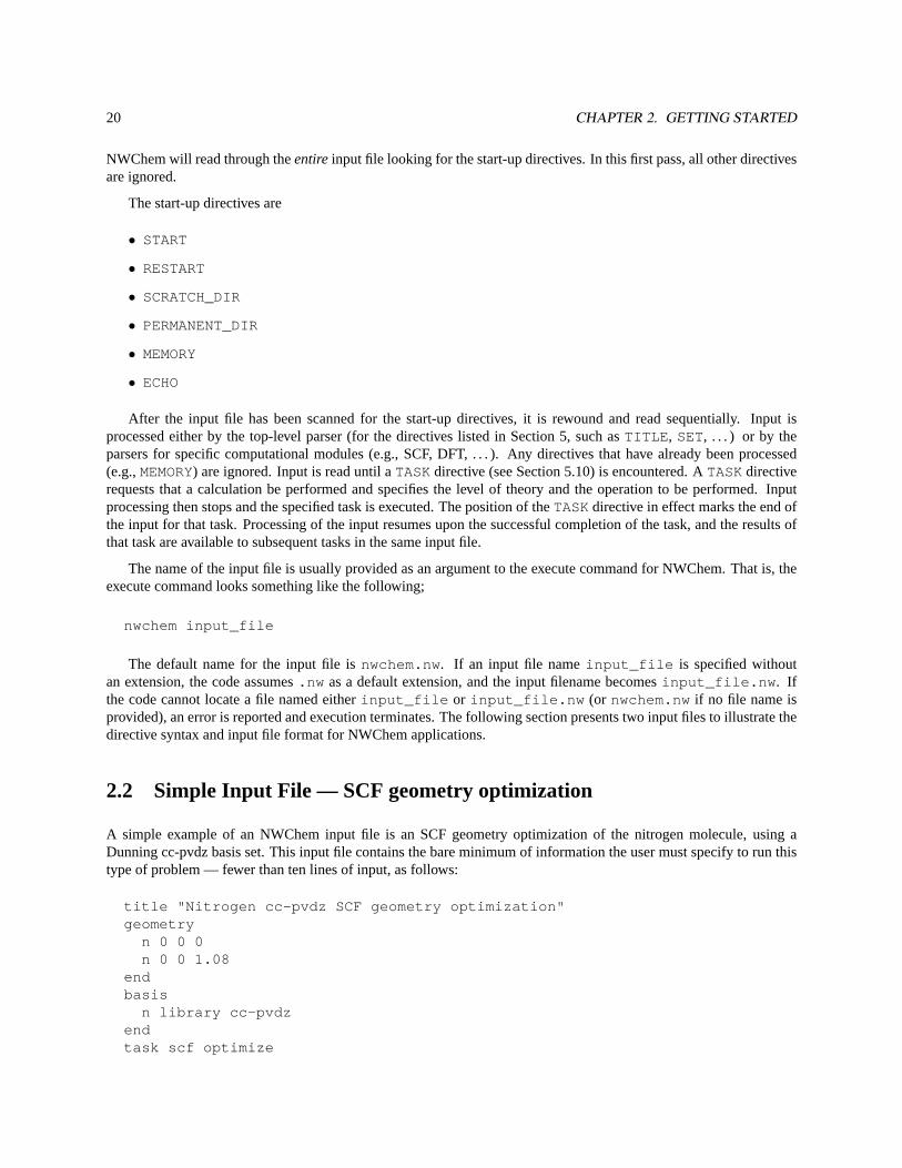
A simple example of an NWChem input file is an SCF geometry optimization of the nitrogen molecule, using aDunning cc-pvdz basis set. This input file contains the bare minimum of information the user must specify to run thistype of problem — fewer than ten lines of input, as follows:
title "Nitrogen cc-pvdz SCF geometry optimization"geometry
n 0 0 0n 0 0 1.08
endbasis
n library cc-pvdzendtask scf optimize
2.3. WATER MOLECULE SAMPLE INPUT FILE 21
Examining the input line by line, it can be seen that it contains only four directives;TITLE , GEOMETRY, BASIS,andTASK. The TITLE directive is optional, and is provided as a means for the user to more easily identify out-puts from different jobs. An initial geometry is specified in Cartesian coordinates and Angstrøms by means of theGEOMETRYdirective. The Dunning cc-pvdz basis is obtained from the NWChem basis library, as specified by theBASIS directive input. TheTASKdirective requests an SCF geometry optimization.
The GEOMETRYdirective (Section 6) defaults to Cartesian coordinates and Angstrøms (options include atomicunits and Z-matrix format; see Section 6.4). The input blocks for theBASIS andGEOMETRYdirectives are structuredin similar fashion, i.e., name, keyword, . . . , end (In this simple example, there are no keywords). TheBASIS inputblock mustcontain basis set information for every atom type in the geometry with which it will be used. Refer toSections 7 and 8, and Appendix A for a description of available basis sets and a discussion of how to define new ones.
The last line of this sample input file (task scf optimize ) tells the program to optimize the moleculargeometry by minimizing the SCF energy. (For a description of possible tasks and the format of theTASKdirective,refer to Section 5.10.)
If the input is stored in the filen2.nw , the command to run this job on a typical UNIX workstation is as follows:
nwchem n2
NWChem output is to UNIX standard output, and error messages are sent to both standard output and standarderror.
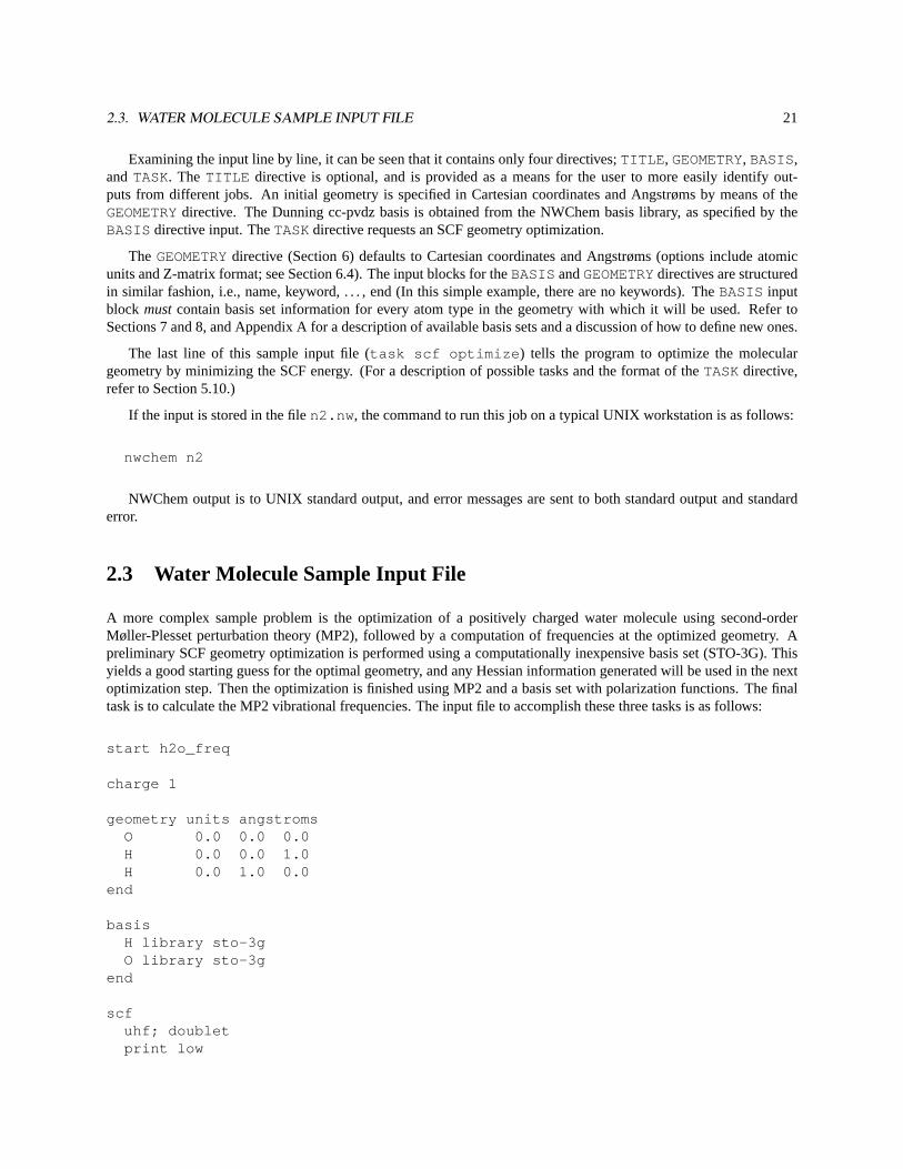
2.3 Water Molecule Sample Input File
A more complex sample problem is the optimization of a positively charged water molecule using second-orderMøller-Plesset perturbation theory (MP2), followed by a computation of frequencies at the optimized geometry. Apreliminary SCF geometry optimization is performed using a computationally inexpensive basis set (STO-3G). Thisyields a good starting guess for the optimal geometry, and any Hessian information generated will be used in the nextoptimization step. Then the optimization is finished using MP2 and a basis set with polarization functions. The finaltask is to calculate the MP2 vibrational frequencies. The input file to accomplish these three tasks is as follows:
start h2o_freq
charge 1
geometry units angstromsO 0.0 0.0 0.0H 0.0 0.0 1.0H 0.0 1.0 0.0
end
basisH library sto-3gO library sto-3g
end
scfuhf; doubletprint low
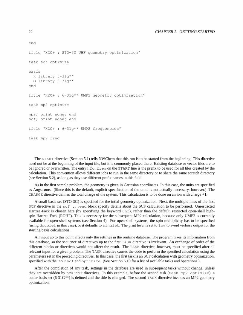
22 CHAPTER 2. GETTING STARTED
end
title "H2O+ : STO-3G UHF geometry optimization"
task scf optimize
basisH library 6-31g**O library 6-31g**
end
title "H2O+ : 6-31g** UMP2 geometry optimization"
task mp2 optimize
mp2; print none; endscf; print none; end
title "H2O+ : 6-31g** UMP2 frequencies"
task mp2 freq
TheSTARTdirective (Section 5.1) tells NWChem that this run is to be started from the beginning. This directiveneed not be at the beginning of the input file, but it is commonly placed there. Existing database or vector files are tobe ignored or overwritten. The entryh2o_freq on theSTARTline is the prefix to be used for all files created by thecalculation. This convention allows different jobs to run in the same directory or to share the same scratch directory(see Section 5.2), as long as they use different prefix names in this field.
As in the first sample problem, the geometry is given in Cartesian coordinates. In this case, the units are specifiedas Angstrøms. (Since this is the default, explicit specification of the units is not actually necessary, however.) TheCHARGEdirective defines the total charge of the system. This calculation is to be done on an ion with charge +1.
A small basis set (STO-3G) is specified for the intial geometry optimization. Next, the multiple lines of the firstSCFdirective in thescf ...end block specify details about the SCF calculation to be performed. UnrestrictedHartree-Fock is chosen here (by specifying the keyworduhf ), rather than the default, restricted open-shell high-spin Hartree-Fock (ROHF). This is necessary for the subsequent MP2 calculation, because only UMP2 is currentlyavailable for open-shell systems (see Section 4). For open-shell systems, the spin multiplicity has to be specified(usingdoublet in this case), or it defaults tosinglet . The print level is set tolow to avoid verbose output for thestarting basis calculations.
All input up to this point affects only the settings in the runtime database. The program takes its information fromthis database, so the sequence of directives up to the firstTASKdirective is irrelevant. An exchange of order of thedifferent blocks or directives would not affect the result. TheTASKdirective, however, must be specified after allrelevant input for a given problem. TheTASKdirective causes the code to perform the specified calculation using theparameters set in the preceding directives. In this case, the first task is an SCF calculation with geometry optimization,specified with the inputscf andoptimize . (See Section 5.10 for a list of available tasks and operations.)
After the completion of any task, settings in the database are used in subsequent tasks without change, unlessthey are overridden by new input directives. In this example, before the second task (task mp2 optimize ), abetter basis set (6-31G**) is defined and the title is changed. The secondTASKdirective invokes an MP2 geometryoptimization.
2.4. INPUT FORMAT AND SYNTAX FOR DIRECTIVES 23
Once the MP2 optimization is completed, the geometry obtained in the calculation is used to perform a frequencycalculation. This task is invoked by the keywordfreq in the finalTASKdirective,task mp2 freq . The secondderivatives of the energy are calculated as numerical derivatives of analytical gradients. The intermediate energiesand gradients are not of interest in this case, so output from the SCF and MP2 modules is disabled with thePRINTdirectives.
2.4 Input Format and Syntax for Directives
This section describes the input format and the syntax used in the rest of this documentation to describe the formatof directives. The input format for the directives used in NWChem is similar to that of UNIX shells, which is alsoused in other chemistry packages, most notably GAMESS-UK. An input line is parsed into whitespace (blanks ortabs) separating tokens or fields. Any token that contains whitespace must be enclosed in double quotes in order to beprocessed correctly. For example, the basis set with the descriptive namemodified Dunning DZ must appear ina directive as"modified Dunning DZ" , since the name consists of three separate words.
2.4.1 Input Format
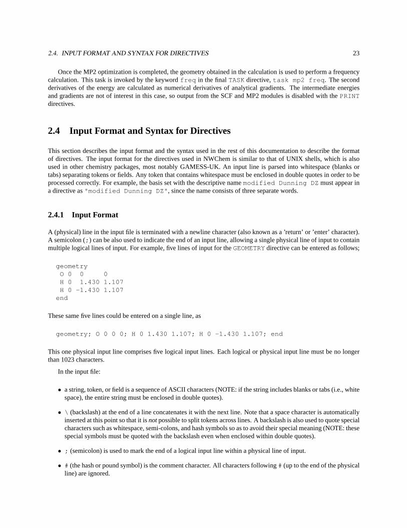
A (physical) line in the input file is terminated with a newline character (also known as a ’return’ or ’enter’ character).A semicolon (; ) can be also used to indicate the end of an input line, allowing a single physical line of input to containmultiple logical lines of input. For example, five lines of input for theGEOMETRYdirective can be entered as follows;
geometryO 0 0 0H 0 1.430 1.107H 0 -1.430 1.107
end
These same five lines could be entered on a single line, as
geometry; O 0 0 0; H 0 1.430 1.107; H 0 -1.430 1.107; end
This one physical input line comprises five logical input lines. Each logical or physical input line must be no longerthan 1023 characters.
In the input file:
• a string, token, or field is a sequence of ASCII characters (NOTE: if the string includes blanks or tabs (i.e., whitespace), the entire string must be enclosed in double quotes).
• \ (backslash) at the end of a line concatenates it with the next line. Note that a space character is automaticallyinserted at this point so that it isnotpossible to split tokens across lines. A backslash is also used to quote specialcharacters such as whitespace, semi-colons, and hash symbols so as to avoid their special meaning (NOTE: thesespecial symbols must be quoted with the backslash even when enclosed within double quotes).
• ; (semicolon) is used to mark the end of a logical input line within a physical line of input.
• # (the hash or pound symbol) is the comment character. All characters following# (up to the end of the physicalline) are ignored.
24 CHAPTER 2. GETTING STARTED
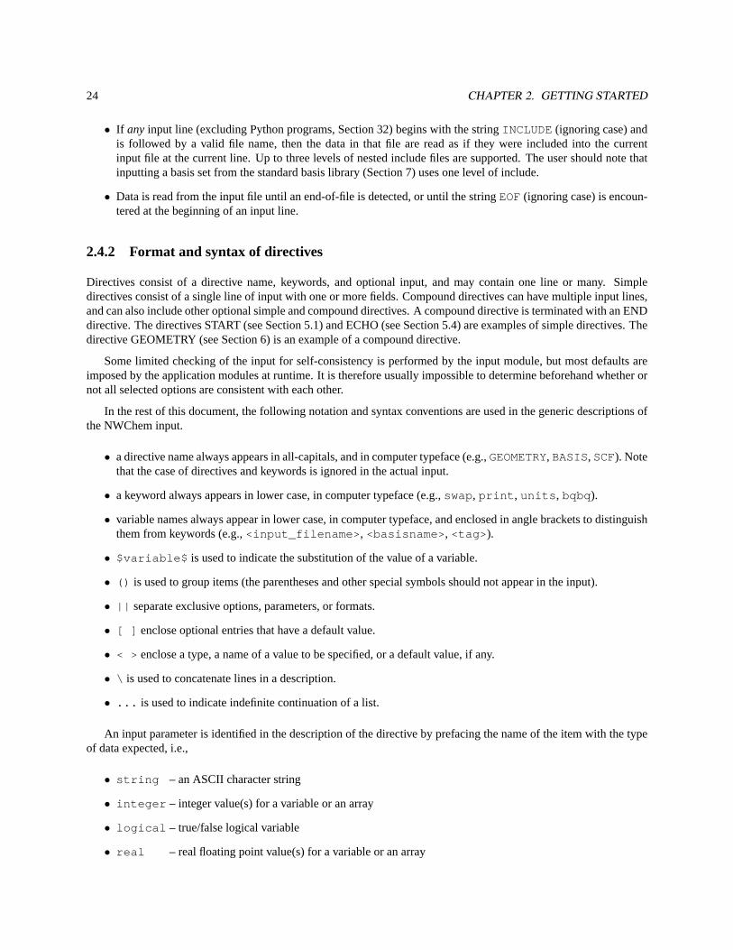
• If any input line (excluding Python programs, Section 32) begins with the stringINCLUDE(ignoring case) andis followed by a valid file name, then the data in that file are read as if they were included into the currentinput file at the current line. Up to three levels of nested include files are supported. The user should note thatinputting a basis set from the standard basis library (Section 7) uses one level of include.
• Data is read from the input file until an end-of-file is detected, or until the stringEOF(ignoring case) is encoun-tered at the beginning of an input line.
2.4.2 Format and syntax of directives
Directives consist of a directive name, keywords, and optional input, and may contain one line or many. Simpledirectives consist of a single line of input with one or more fields. Compound directives can have multiple input lines,and can also include other optional simple and compound directives. A compound directive is terminated with an ENDdirective. The directives START (see Section 5.1) and ECHO (see Section 5.4) are examples of simple directives. Thedirective GEOMETRY (see Section 6) is an example of a compound directive.
Some limited checking of the input for self-consistency is performed by the input module, but most defaults areimposed by the application modules at runtime. It is therefore usually impossible to determine beforehand whether ornot all selected options are consistent with each other.
In the rest of this document, the following notation and syntax conventions are used in the generic descriptions ofthe NWChem input.
• a directive name always appears in all-capitals, and in computer typeface (e.g.,GEOMETRY, BASIS, SCF). Notethat the case of directives and keywords is ignored in the actual input.
• a keyword always appears in lower case, in computer typeface (e.g.,swap, print , units , bqbq ).
• variable names always appear in lower case, in computer typeface, and enclosed in angle brackets to distinguishthem from keywords (e.g.,<input_filename> , <basisname> , <tag> ).
• $variable$ is used to indicate the substitution of the value of a variable.
• () is used to group items (the parentheses and other special symbols should not appear in the input).
• || separate exclusive options, parameters, or formats.
• [ ] enclose optional entries that have a default value.
• < > enclose a type, a name of a value to be specified, or a default value, if any.
• \ is used to concatenate lines in a description.
• ... is used to indicate indefinite continuation of a list.
An input parameter is identified in the description of the directive by prefacing the name of the item with the typeof data expected, i.e.,
• string – an ASCII character string
• integer – integer value(s) for a variable or an array
• logical – true/false logical variable
• real – real floating point value(s) for a variable or an array
2.4. INPUT FORMAT AND SYNTAX FOR DIRECTIVES 25
• double – synonymous with real
If an input item is not prefaced by one of these type names, it is assumed to be of type “string”.
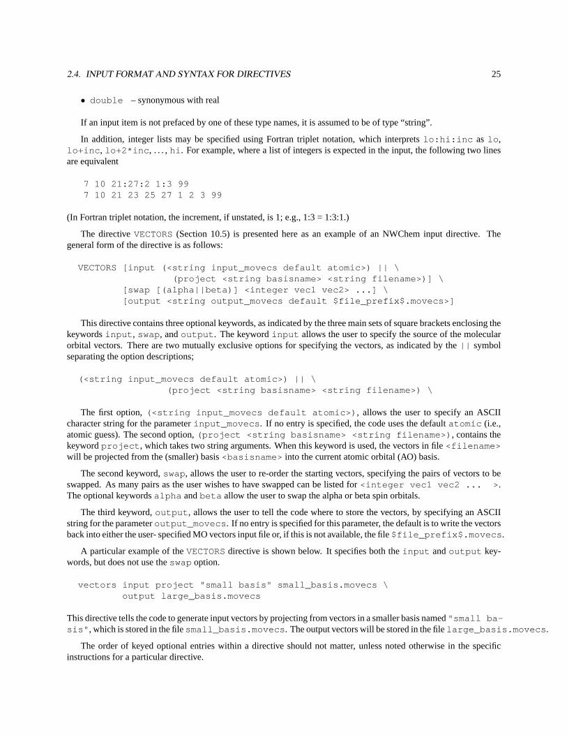
In addition, integer lists may be specified using Fortran triplet notation, which interpretslo:hi:inc as lo ,lo+inc , lo+2*inc , . . . ,hi . For example, where a list of integers is expected in the input, the following two linesare equivalent
7 10 21:27:2 1:3 997 10 21 23 25 27 1 2 3 99
(In Fortran triplet notation, the increment, if unstated, is 1; e.g., 1:3 = 1:3:1.)
The directiveVECTORS(Section 10.5) is presented here as an example of an NWChem input directive. Thegeneral form of the directive is as follows:
VECTORS [input (<string input_movecs default atomic>) || \(project <string basisname> <string filename>)] \
[swap [(alpha||beta)] <integer vec1 vec2> ...] \[output <string output_movecs default $file_prefix$.movecs>]
This directive contains three optional keywords, as indicated by the three main sets of square brackets enclosing thekeywordsinput , swap, andoutput . The keywordinput allows the user to specify the source of the molecularorbital vectors. There are two mutually exclusive options for specifying the vectors, as indicated by the|| symbolseparating the option descriptions;
(<string input_movecs default atomic>) || \(project <string basisname> <string filename>) \
The first option,(<string input_movecs default atomic>) , allows the user to specify an ASCIIcharacter string for the parameterinput_movecs . If no entry is specified, the code uses the defaultatomic (i.e.,atomic guess). The second option,(project <string basisname> <string filename>) , contains thekeywordproject , which takes two string arguments. When this keyword is used, the vectors in file<filename>will be projected from the (smaller) basis<basisname> into the current atomic orbital (AO) basis.
The second keyword,swap, allows the user to re-order the starting vectors, specifying the pairs of vectors to beswapped. As many pairs as the user wishes to have swapped can be listed for<integer vec1 vec2 ... > .The optional keywordsalpha andbeta allow the user to swap the alpha or beta spin orbitals.
The third keyword,output , allows the user to tell the code where to store the vectors, by specifying an ASCIIstring for the parameteroutput_movecs . If no entry is specified for this parameter, the default is to write the vectorsback into either the user- specified MO vectors input file or, if this is not available, the file$file_prefix$.movecs .
A particular example of theVECTORSdirective is shown below. It specifies both theinput andoutput key-words, but does not use theswap option.
vectors input project "small basis" small_basis.movecs \output large_basis.movecs
This directive tells the code to generate input vectors by projecting from vectors in a smaller basis named"small ba-sis" , which is stored in the filesmall_basis.movecs . The output vectors will be stored in the filelarge_basis.movecs .
The order of keyed optional entries within a directive should not matter, unless noted otherwise in the specificinstructions for a particular directive.

26 CHAPTER 2. GETTING STARTED
Chapter 3
NWChem Architecture
As noted above, NWChem consists of independent modules that perform the various functions of the code. Examplesinclude the input parser, self-consistent field (SCF) energy, SCF analytic gradient, and density functional theory (DFT)energy modules. The independent NWChem modules can share data only through a disk-resident database, which issimilar to the GAMESS-UK dumpfile or the Gaussian checkpoint file. This allows the modules to share data, or toshare access to files containing data.
It is not necessary for the user to be intimately familiar with the contents of the database in order to run NWChem.However, a nodding acquaintance with the design of the code will help in clarifying the logic behind the input re-quirements, especially when restarting jobs or performing multiple tasks within one job. Section 3.1 gives a generaldescription of the database.
As described above (Section 2.1), all start-up directives are processed at the beginning of the job by the mainprogram, and then the input module is invoked. Each input directive usually results in one or more entries being madein the database. When aTASKdirective is encountered, control is passed to the appropriate module, which extractsrelevant data from the database and any associated files. Upon completion of the task, the module will store significantresults in the database, and may also modify other database entries in order to affect the behavior of subsequentcomputations.
3.1 Database Structure
Data is shared between modules of NWChem by means of the database. Three main types of information are storedin the data base: (1) arrays of data, (2) names of files that contain data, and (3) objects. Arrays are stored directly inthe database, and contain the following information:
1. the name of the array, which is a string of ASCII characters (e.g.,"reference energies" )
2. the type of the data in the array (i.e., real, integer, logical, or character)
3. the number (N) of data items in the array (Note: A scalar is stored as an array of unit length.)
4. the N items of data of the specified type
It is possible to enter data directly into the database using theSETdirective (see Section 5.7). For example, to storea (64-bit precision) three-element real array with the name"reference energies" in the database, the directiveis as follows:
27
28 CHAPTER 3. NWCHEM ARCHITECTURE
set "reference energies" 0.0 1.0 -76.2
NWChem determines the data to be real (based on the type of the first element,0.0 ), counts the number of elementsin the array, and enters the array into the database.
Much of the data stored in the database is internally managed by NWChem and should not be modified by the user.However, other data, including some NWChem input options, can be freely modified.
Objects are built in the database by storing associated data as multiple entries, using an internally consistentnaming convention. This data is managed exclusively by the subroutines (or methods) that are associated with theobject. Currently, the code has two main objects: basis sets and geometries. Sections 6 and 7 present a completediscussion of the input to describe these objects.
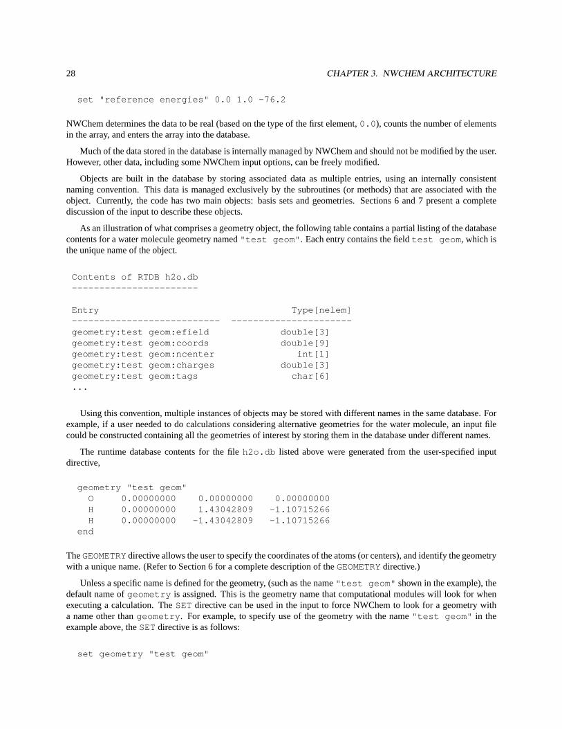
As an illustration of what comprises a geometry object, the following table contains a partial listing of the databasecontents for a water molecule geometry named"test geom" . Each entry contains the fieldtest geom , which isthe unique name of the object.
Contents of RTDB h2o.db-----------------------
Entry Type[nelem]--------------------------- ----------------------geometry:test geom:efield double[3]geometry:test geom:coords double[9]geometry:test geom:ncenter int[1]geometry:test geom:charges double[3]geometry:test geom:tags char[6]...
Using this convention, multiple instances of objects may be stored with different names in the same database. Forexample, if a user needed to do calculations considering alternative geometries for the water molecule, an input filecould be constructed containing all the geometries of interest by storing them in the database under different names.
The runtime database contents for the fileh2o.db listed above were generated from the user-specified inputdirective,
geometry "test geom"O 0.00000000 0.00000000 0.00000000H 0.00000000 1.43042809 -1.10715266H 0.00000000 -1.43042809 -1.10715266
end
TheGEOMETRYdirective allows the user to specify the coordinates of the atoms (or centers), and identify the geometrywith a unique name. (Refer to Section 6 for a complete description of theGEOMETRYdirective.)
Unless a specific name is defined for the geometry, (such as the name"test geom" shown in the example), thedefault name ofgeometry is assigned. This is the geometry name that computational modules will look for whenexecuting a calculation. TheSET directive can be used in the input to force NWChem to look for a geometry witha name other thangeometry . For example, to specify use of the geometry with the name"test geom" in theexample above, theSETdirective is as follows:
set geometry "test geom"

3.2. PERSISTENCE OF DATA AND RESTART 29
NWChem will automatically check for such indirections when loading geometries. Storage of data associated withbasis sets, the other database resident object, functions in a similar fashion, using the default name"ao basis" .
3.2 Persistence of data and restart
The database is persistent, meaning that all input data and output data (calculation results) that are not destroyed in thecourse of execution are permanently stored. These data are therefore available to subsequent tasks or jobs. This makesthe input for restart jobs very simple, since only new or changed data must be provided. It also makes the behavior ofsuccessive restart jobsidenticalto that of multiple tasks within one job.
Sometimes, however, this persistence is undesirable, and it is necessary to return an NWChem module to its defaultbehavior by restoring the database to its input-free state. In such a case, theUNSETdirective (see Section 5.8) can beused to delete all database entries associated with a given module (including both inputs and outputs).

30 CHAPTER 3. NWCHEM ARCHITECTURE
Chapter 4
Functionality
NWChem provides many methods to compute the properties of molecular and periodic systems using standard quan-tum mechanical descriptions of the electronic wavefunction or density. In addition, NWChem has the capability toperform classical molecular dynamics and free energy simulations. These approaches may be combined to performmixed quantum-mechanics and molecular-mechanics simulations.
NWChem is available on almost all high performance computing platforms, workstations, PCs running LINUX,as well as clusters of desktop platforms or workgroup servers. NWChem development has been devoted to providingmaximum efficiency on massively parallel processors. It achieves this performance on the 512 node IBM SP system inthe EMSL’s MSCF and on the 512 node CRAY T3E-900 system in the National Energy Research Scientific ComputingCenter. It has not been optimized for high performance on single processor desktop systems.
4.1 Molecular electronic structure
The following quantum mechanical methods are available to calculate energies and analytic first derivatives withrespect to atomic coordinates. Second derivatives are computed by finite difference of the first derivatives.
• Self Consistent Field (SCF) or Hartree Fock (RHF, UHF, high-spin ROHF).
• Gaussian Density Functional Theory (DFT), using many local and non-local exchange-correlation potentials(RHF or UHF) with formalN3 andN4 scaling.
• Spin-orbit DFT (SODFT), using many local and non-local exchange-correlation potentials (UHF).
• MP2 including semi-direct using frozen core and RHF and UHF reference.
• Complete active space SCF (CASSCF).
The following methods are available to compute energies only. First and second derivatives are computed by finitedifference of the energies.
• CCSD, CCSD(T), CCSD+T(CCSD), with RHF reference.
• Selected-CI with second-order perturbation correction.
• MP2 fully-direct with RHF reference.
31

32 CHAPTER 4. FUNCTIONALITY
• Resolution of the identity integral approximation MP2 (RI-MP2), with RHF and UHF reference.
For all methods, the following operations may be performed:
• Single point energy
• Geometry optimization (minimization and transition state)
• Molecular dynamics on the fullyab initio potential energy surface
• Numerical first and second derivatives automatically computed if analytic derivatives are not available
• Normal mode vibrational analysis in cartesian coordinates
• ONIOM hybrid method of Morokuma and co-workers
• Generation of the electron density file for graphical display
• Evaluation of static, one-electron properties.
• Electrostatic potential fit of atomic partial charges (CHELPG method with optional RESP restraints or chargeconstraints)
For closed and open shell SCF and DFT:
• COSMO energies - the continuum solvation ’Conductor-Like Screening’ Model of A. Klamt and G. Schuurmannto describe dielectric screening effects in solvents.
In addition, automatic interfaces are provided to
• The COLUMBUS multi-reference CI package
• The natural bond orbital (NBO) package
• Python
4.2 Relativistic effects
The following methods for including relativity in quantum chemistry calculations are available:
• The spin-free one-electron Douglas-Kroll approximation is available for all quantum mechanical methods andtheir gradients.
• Dyall’s spin-free Modified Dirac Hamiltonian approximation is available for the Hartree-Fock method and itsgradients.
• One-electron spin-orbit effects can be included via spin-orbit potentials. This option is available for DFT andits gradients, but has to be run without symmetry.
4.3. PSEUDOPOTENTIAL PLANE-WAVE ELECTRONIC STRUCTURE 33
4.3 Pseudopotential plane-wave electronic structure
The following modules are available to compute the energy, minimize the geometry and perform ab initio moleculardynamics using pseudopotential plane-wave DFT.
• Fixed step length steepest descent
• Conuugate Gradient
• Car-Parrinello (extended Lagrangian dynamics)
With
• Vosko and PBE96 exchange-correlation potentials (restricted and unrestricted)
• (Gamma point) Periodic orthorhombic simulation cells for calculating molecules, liquids, crystals, and surfaces
• Aperiodic orthorhombic simulations cells for calculating molecules that are charged or highly polar
• Constant energy and constant temperature Car-Parrinello simulations
• Hamann and Troullier-Martins norm-conserving pseudopotentials with opt ional semicore corrections
• Modules to convert between small and large plane-wave expansions
• Interface to DRIVER, STEPPER, and VIB modules
• Mulliken analysis
4.4 Periodic system electronic structure
A module (Gaussian Approach to Polymers, Surfaces and Solids (GAPSS)) is available to compute energies by Gaus-sian Density Functional Theory (DFT) with many local and non-local exchange-correlation potentials.
4.5 Molecular dynamics
The following functionality is available for classical molecular simulations:
• Single configuration energy evaluation
• Energy minimization
• Molecular dynamics simulation
• Free energy simulation (multistep thermodynamic perturbation (MSTP) or multiconfiguration thermodynamicintegration (MCTI) methods with options of single and/or dual topologies, double wide sampling, and separation-shifted scaling)
The classical force field includes:
• Effective pair potentials (functional form used in AMBER, GROMOS, CHARMM, etc.)
34 CHAPTER 4. FUNCTIONALITY
• First order polarization
• Self consistent polarization
• Smooth particle mesh Ewald (SPME)
• Twin range energy and force evaluation
• Periodic boundary conditions
• SHAKE constraints
• Consistent temperature and/or pressure ensembles
NWChem also has the capability to combine classical and quantum descriptions in order to perform:
• Mixed quantum-mechanics and molecular-mechanics (QM/MM) minimizations and molecular dynamics simu-lation , and
• Quantum molecular dynamics simulation by using any of the quantum mechanical methods capable of returninggradients.
4.6 Python
The Python programming language has been embedded within NWChem and many of the high level capabilities ofNWChem can be easily combined and controlled by the user to perform complex operations.
4.7 Parallel tools and libraries (ParSoft)
• Global arrays (GA)
• Agregate Remote Memory Copy Interface (ARMCI)
• Linear Algebra (PeIGS) and FFT
• ParIO
• Memory allocation (MA)
Chapter 5
Top-level directives
Top-level directives are directives that can affect all modules in the code. Some specify molecular properties (e.g.,total charge) or other data that should apply to all subsequent calculations with the current database. However, mosttop-level directives provide the user with the means to manage the resources for a calculation and to start computations.As the first step in the execution of a job, NWChem scans the entire input file looking for start-up directives, whichNWChem must process before all other input. The input file is then rewound and processed sequentially, and eachdirective is processed in the order in which it is encountered. In this second pass, start-up directives are ignored.
The following sections describe each of the top-level directives in detail, noting all keywords, options, requiredinput, and defaults.
5.1 START and RESTART — Start-up mode
A STARTor RESTARTdirective is optional. If one of these two directives is not specified explicitly, the code willinfer one, based upon the name of the input file and the availability of the database. When allowing NWChem to inferthe start-up directive, the user must be quite certain that the contents of the database will result in the desired action.It is usually more prudent to specify the directive explicitly, using the following format:
(RESTART || START) \[<string file_prefix default $input_file_prefix$>] \[rtdb <string rtdb_file_name default $file_prefix$.db>]
The STARTdirective indicates that the calculation is one in which a new database is to be created. Any rel-evant information that already exists in a previous database of the same name is destroyed. The string variable<file_prefix> will be used as the prefix to name any files created in the course of the calculation.
E.g., to start a new calculation on water, one might specify
start water
which would result in all files beginning with"water." .
If the user does not specify an entry for<file_prefix> on theSTARTdirective (or omits theSTARTdirectivealtogether), the code uses the base-name of the input file as the file prefix. That is, the variable<file_prefix>is assigned the name of the input file (not its full pathname), but without the last "dot-suffix". For example, the input
35
36 CHAPTER 5. TOP-LEVEL DIRECTIVES
file name/home/dave/job.2.nw yields job.2 as the file prefix, if a name is not assigned explicitly using theSTARTdirective.
The user also has the option of specifying a unique name for the database, using the keywordrtdb . When thiskeyword is entered, the string entered forrtdb_file_name is used as the database name. If the keywordrtbd isomitted, the name of the database defaults to$<file_prefix>$.db in the directory for permanent files.
If a calculation is to start from a previous calculation and go on using the existing database, theRESTARTdirectivemust be used. In such a case, the previous database must already exist. The name specified for<file_prefix>usually should not be changed when restarting a calculation. If it is changed, NWChem will not be able to find neededfiles when going on with the calculation.
In the most common situation, the previous calculation was completed (with or without an error condition), and itis desired to perform a new task or restart the previous one, perhaps with some input changes. In these instances, theRESTARTdirective should be used. This reuses the previous database and associated files, and reads the input file fornew input and task information.
TheRESTARTdirective looks immediately for new input and task information, deleting information about previ-ous incomplete tasks.
To summarize the default options for this start-up directive, if the input file doesnot contain aSTARTor aRESTARTdirective, then
• the variable<file_prefix> is assigned the name of the input file for the job, without the suffix (which isusually.nw )
• the variable<rtdb_file_name> is assigned the default name,$file_prefix$.db
If the database with name$file_prefix$.db doesnot already exist, the calculation is carried out as if aSTARTdirective had been encountered. If the database with name$file_prefix$.db doesexist, then the calculation isperformed as if aRESTARTdirective had been encountered.
For example, NWChem can be run using an input file with the namewater.nw by typing the UNIX commandline,
nwchem water.nw
If the NWChem input filewater.nw does not contain aSTARTor RESTARTdirective, the code sets the vari-able<file_prefix> to water . Files created by the job will have this prefix, and the database will be namedwater.db . If the databasewater.db doesnot exist already, the code behaves as if the input file contains thedirective,
start water
If the databasewater.db doesexist, the code behaves as if the input file contained the directive,
restart water
5.2 SCRATCH_DIR and PERMANENT_DIR — File directories
These are start-up directives that allow the user to specify the directory location of scratch and permanent files createdby NWChem. NWChem distinguishes between permanent (or persistent) files and scratch (or temporary) files, and
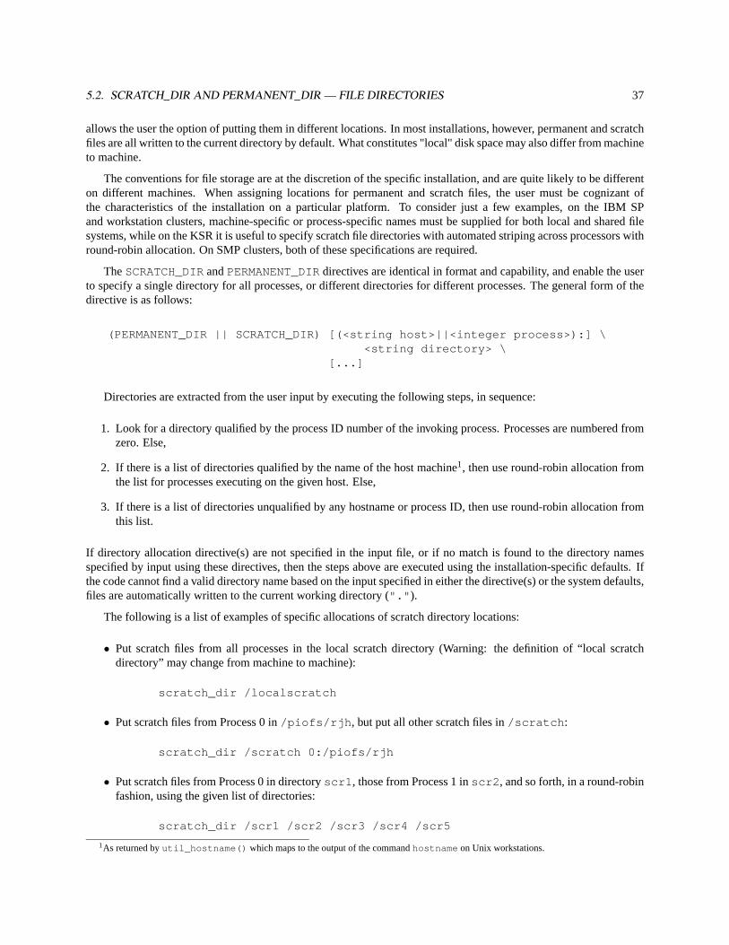
5.2. SCRATCH_DIR AND PERMANENT_DIR — FILE DIRECTORIES 37
allows the user the option of putting them in different locations. In most installations, however, permanent and scratchfiles are all written to the current directory by default. What constitutes "local" disk space may also differ from machineto machine.
The conventions for file storage are at the discretion of the specific installation, and are quite likely to be differenton different machines. When assigning locations for permanent and scratch files, the user must be cognizant ofthe characteristics of the installation on a particular platform. To consider just a few examples, on the IBM SPand workstation clusters, machine-specific or process-specific names must be supplied for both local and shared filesystems, while on the KSR it is useful to specify scratch file directories with automated striping across processors withround-robin allocation. On SMP clusters, both of these specifications are required.
TheSCRATCH_DIRandPERMANENT_DIRdirectives are identical in format and capability, and enable the userto specify a single directory for all processes, or different directories for different processes. The general form of thedirective is as follows:
(PERMANENT_DIR || SCRATCH_DIR) [(<string host>||<integer process>):] \<string directory> \
[...]
Directories are extracted from the user input by executing the following steps, in sequence:
1. Look for a directory qualified by the process ID number of the invoking process. Processes are numbered fromzero. Else,
2. If there is a list of directories qualified by the name of the host machine1, then use round-robin allocation fromthe list for processes executing on the given host. Else,
3. If there is a list of directories unqualified by any hostname or process ID, then use round-robin allocation fromthis list.
If directory allocation directive(s) are not specified in the input file, or if no match is found to the directory namesspecified by input using these directives, then the steps above are executed using the installation-specific defaults. Ifthe code cannot find a valid directory name based on the input specified in either the directive(s) or the system defaults,files are automatically written to the current working directory ("." ).
The following is a list of examples of specific allocations of scratch directory locations:
• Put scratch files from all processes in the local scratch directory (Warning: the definition of “local scratchdirectory” may change from machine to machine):
scratch_dir /localscratch
• Put scratch files from Process 0 in/piofs/rjh , but put all other scratch files in/scratch :
scratch_dir /scratch 0:/piofs/rjh
• Put scratch files from Process 0 in directoryscr1 , those from Process 1 inscr2 , and so forth, in a round-robinfashion, using the given list of directories:
scratch_dir /scr1 /scr2 /scr3 /scr4 /scr5
1As returned byutil_hostname() which maps to the output of the commandhostname on Unix workstations.
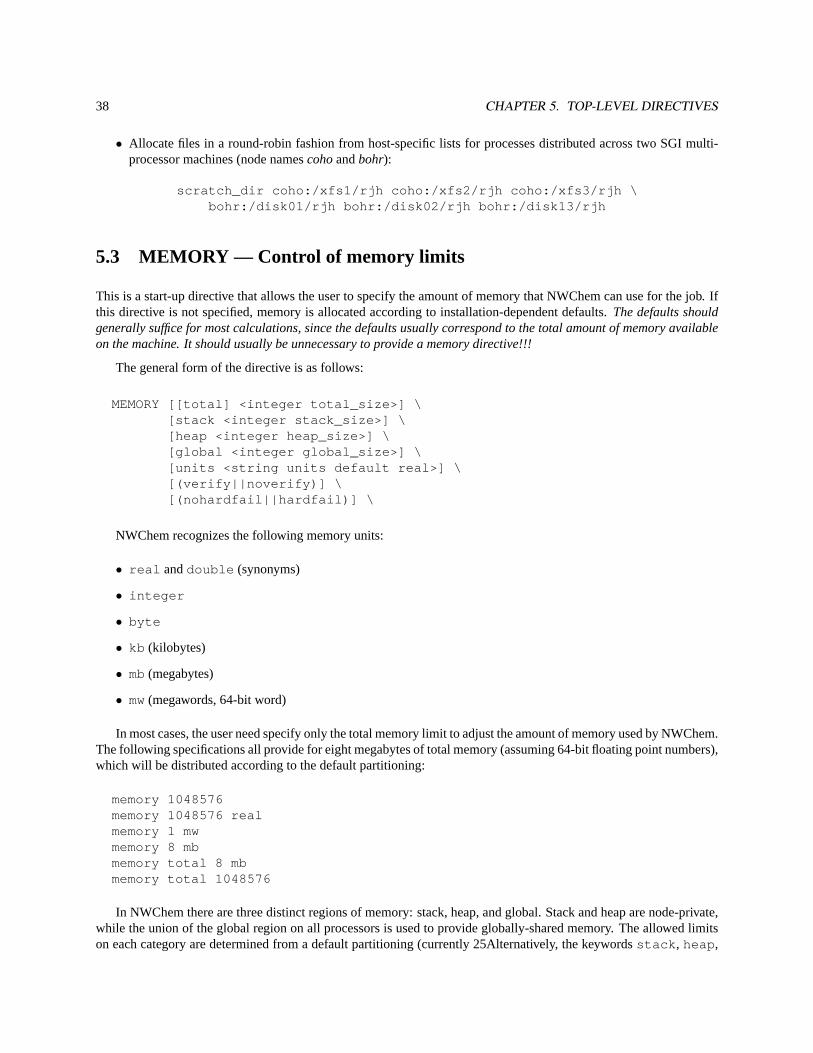
38 CHAPTER 5. TOP-LEVEL DIRECTIVES
• Allocate files in a round-robin fashion from host-specific lists for processes distributed across two SGI multi-processor machines (node namescohoandbohr):
scratch_dir coho:/xfs1/rjh coho:/xfs2/rjh coho:/xfs3/rjh \bohr:/disk01/rjh bohr:/disk02/rjh bohr:/disk13/rjh
5.3 MEMORY — Control of memory limits
This is a start-up directive that allows the user to specify the amount of memory that NWChem can use for the job. Ifthis directive is not specified, memory is allocated according to installation-dependent defaults.The defaults shouldgenerally suffice for most calculations, since the defaults usually correspond to the total amount of memory availableon the machine. It should usually be unnecessary to provide a memory directive!!!
The general form of the directive is as follows:
MEMORY [[total] <integer total_size>] \[stack <integer stack_size>] \[heap <integer heap_size>] \[global <integer global_size>] \[units <string units default real>] \[(verify||noverify)] \[(nohardfail||hardfail)] \
NWChem recognizes the following memory units:
• real anddouble (synonyms)
• integer
• byte
• kb (kilobytes)
• mb(megabytes)
• mw(megawords, 64-bit word)
In most cases, the user need specify only the total memory limit to adjust the amount of memory used by NWChem.The following specifications all provide for eight megabytes of total memory (assuming 64-bit floating point numbers),which will be distributed according to the default partitioning:
memory 1048576memory 1048576 realmemory 1 mwmemory 8 mbmemory total 8 mbmemory total 1048576
In NWChem there are three distinct regions of memory: stack, heap, and global. Stack and heap are node-private,while the union of the global region on all processors is used to provide globally-shared memory. The allowed limitson each category are determined from a default partitioning (currently 25Alternatively, the keywordsstack , heap ,
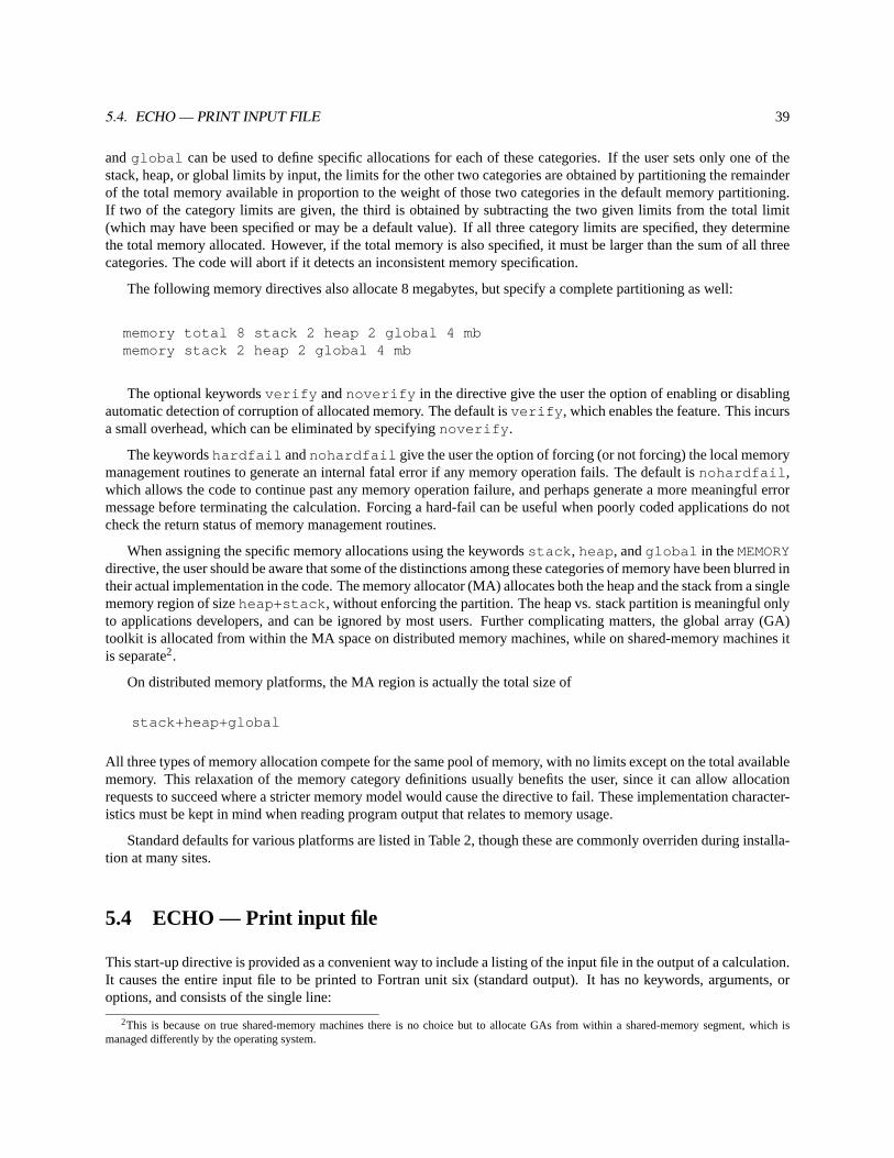
5.4. ECHO — PRINT INPUT FILE 39
andglobal can be used to define specific allocations for each of these categories. If the user sets only one of thestack, heap, or global limits by input, the limits for the other two categories are obtained by partitioning the remainderof the total memory available in proportion to the weight of those two categories in the default memory partitioning.If two of the category limits are given, the third is obtained by subtracting the two given limits from the total limit(which may have been specified or may be a default value). If all three category limits are specified, they determinethe total memory allocated. However, if the total memory is also specified, it must be larger than the sum of all threecategories. The code will abort if it detects an inconsistent memory specification.
The following memory directives also allocate 8 megabytes, but specify a complete partitioning as well:
memory total 8 stack 2 heap 2 global 4 mbmemory stack 2 heap 2 global 4 mb
The optional keywordsverify andnoverify in the directive give the user the option of enabling or disablingautomatic detection of corruption of allocated memory. The default isverify , which enables the feature. This incursa small overhead, which can be eliminated by specifyingnoverify .
The keywordshardfail andnohardfail give the user the option of forcing (or not forcing) the local memorymanagement routines to generate an internal fatal error if any memory operation fails. The default isnohardfail ,which allows the code to continue past any memory operation failure, and perhaps generate a more meaningful errormessage before terminating the calculation. Forcing a hard-fail can be useful when poorly coded applications do notcheck the return status of memory management routines.
When assigning the specific memory allocations using the keywordsstack , heap , andglobal in theMEMORYdirective, the user should be aware that some of the distinctions among these categories of memory have been blurred intheir actual implementation in the code. The memory allocator (MA) allocates both the heap and the stack from a singlememory region of sizeheap+stack , without enforcing the partition. The heap vs. stack partition is meaningful onlyto applications developers, and can be ignored by most users. Further complicating matters, the global array (GA)toolkit is allocated from within the MA space on distributed memory machines, while on shared-memory machines itis separate2.
On distributed memory platforms, the MA region is actually the total size of
stack+heap+global
All three types of memory allocation compete for the same pool of memory, with no limits except on the total availablememory. This relaxation of the memory category definitions usually benefits the user, since it can allow allocationrequests to succeed where a stricter memory model would cause the directive to fail. These implementation character-istics must be kept in mind when reading program output that relates to memory usage.
Standard defaults for various platforms are listed in Table 2, though these are commonly overriden during installa-tion at many sites.
5.4 ECHO — Print input file
This start-up directive is provided as a convenient way to include a listing of the input file in the output of a calculation.It causes the entire input file to be printed to Fortran unit six (standard output). It has no keywords, arguments, oroptions, and consists of the single line:
2This is because on true shared-memory machines there is no choice but to allocate GAs from within a shared-memory segment, which ismanaged differently by the operating system.
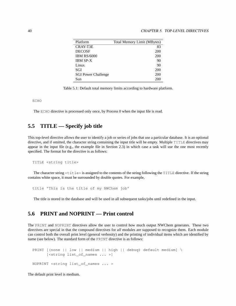
40 CHAPTER 5. TOP-LEVEL DIRECTIVES
Platform Total Memory Limit (MBytes)CRAY-T3E 83DECOSF 200IBM RS/6000 200IBM SP-X 90Linux 90SGI 200SGI Power Challenge 200Sun 200
Table 5.1: Default total memory limits according to hardware platform.
ECHO
TheECHOdirective is processed only once, by Process 0 when the input file is read.
5.5 TITLE — Specify job title
This top-level directive allows the user to identify a job or series of jobs that use a particular database. It is an optionaldirective, and if omitted, the character string containing the input title will be empty. MultipleTITLE directives mayappear in the input file (e.g., the example file in Section 2.3) in which case a task will use the one most recentlyspecified. The format for the directive is as follows:
TITLE <string title>
The character string<title> is assigned to the contents of the string following theTITLE directive. If the stringcontains white space, it must be surrounded by double quotes. For example,
title "This is the title of my NWChem job"
The title is stored in the database and will be used in all subsequent tasks/jobs until redefined in the input.
5.6 PRINT and NOPRINT — Print control
The PRINT andNOPRINTdirectives allow the user to control how much output NWChem generates. These twodirectives are special in that the compound directives forall modules are supposed to recognize them. Each modulecan control both the overall print level (general verbosity) and the printing of individual items which are identified byname (see below). The standard form of thePRINT directive is as follows:
PRINT [(none || low || medium || high || debug) default medium] \[<string list_of_names ... >]
NOPRINT <string list_of_names ... >
The default print level is medium.
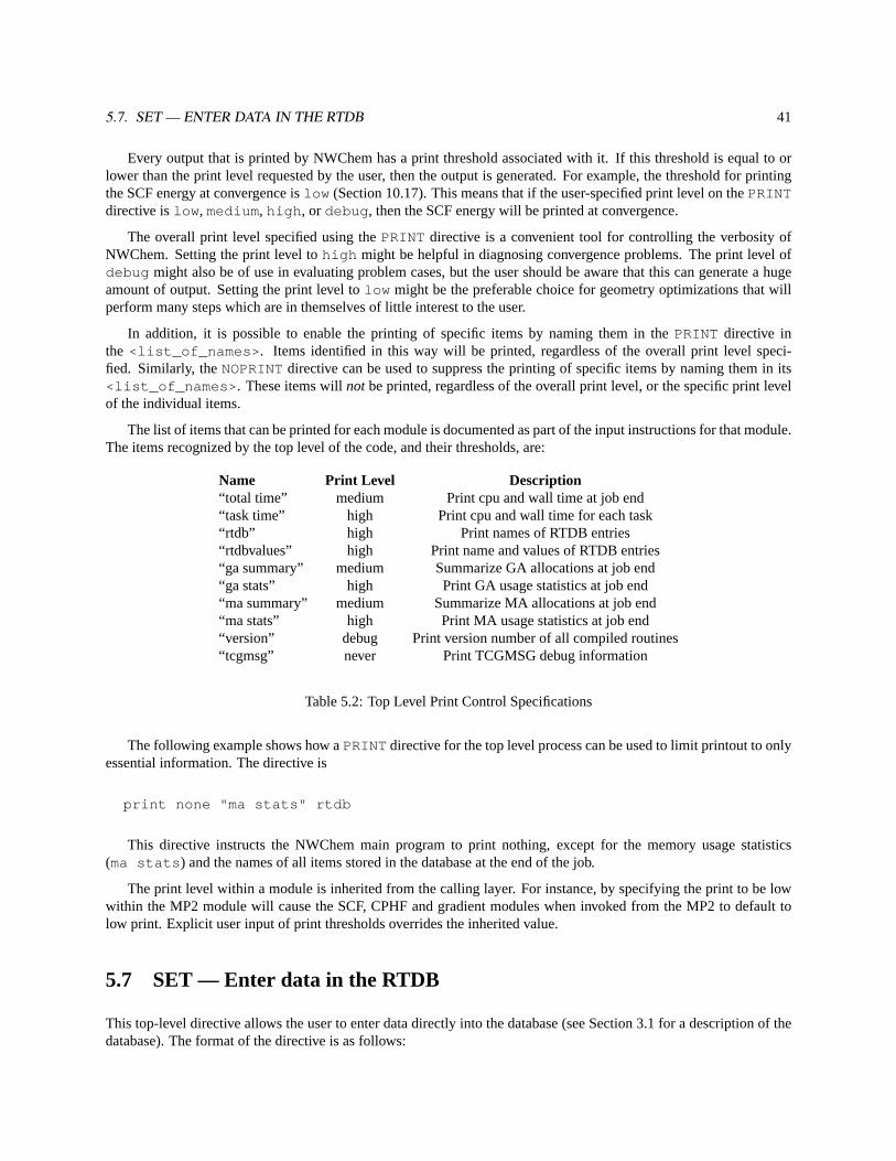
5.7. SET — ENTER DATA IN THE RTDB 41
Every output that is printed by NWChem has a print threshold associated with it. If this threshold is equal to orlower than the print level requested by the user, then the output is generated. For example, the threshold for printingthe SCF energy at convergence islow (Section 10.17). This means that if the user-specified print level on thePRINTdirective islow , medium, high , or debug , then the SCF energy will be printed at convergence.
The overall print level specified using thePRINT directive is a convenient tool for controlling the verbosity ofNWChem. Setting the print level tohigh might be helpful in diagnosing convergence problems. The print level ofdebug might also be of use in evaluating problem cases, but the user should be aware that this can generate a hugeamount of output. Setting the print level tolow might be the preferable choice for geometry optimizations that willperform many steps which are in themselves of little interest to the user.
In addition, it is possible to enable the printing of specific items by naming them in thePRINT directive inthe <list_of_names> . Items identified in this way will be printed, regardless of the overall print level speci-fied. Similarly, theNOPRINTdirective can be used to suppress the printing of specific items by naming them in its<list_of_names> . These items willnot be printed, regardless of the overall print level, or the specific print levelof the individual items.
The list of items that can be printed for each module is documented as part of the input instructions for that module.The items recognized by the top level of the code, and their thresholds, are:
Name Print Level Description“total time” medium Print cpu and wall time at job end“task time” high Print cpu and wall time for each task“rtdb” high Print names of RTDB entries“rtdbvalues” high Print name and values of RTDB entries“ga summary” medium Summarize GA allocations at job end“ga stats” high Print GA usage statistics at job end“ma summary” medium Summarize MA allocations at job end“ma stats” high Print MA usage statistics at job end“version” debug Print version number of all compiled routines“tcgmsg” never Print TCGMSG debug information
Table 5.2: Top Level Print Control Specifications
The following example shows how aPRINT directive for the top level process can be used to limit printout to onlyessential information. The directive is
print none "ma stats" rtdb
This directive instructs the NWChem main program to print nothing, except for the memory usage statistics(ma stats ) and the names of all items stored in the database at the end of the job.
The print level within a module is inherited from the calling layer. For instance, by specifying the print to be lowwithin the MP2 module will cause the SCF, CPHF and gradient modules when invoked from the MP2 to default tolow print. Explicit user input of print thresholds overrides the inherited value.
5.7 SET — Enter data in the RTDB
This top-level directive allows the user to enter data directly into the database (see Section 3.1 for a description of thedatabase). The format of the directive is as follows:
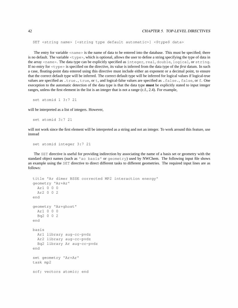
42 CHAPTER 5. TOP-LEVEL DIRECTIVES
SET <string name> [<string type default automatic>] <$type$ data>
The entry for variable<name> is the name of data to be entered into the database. This must be specified; thereis no default. The variable<type> , which is optional, allows the user to define a string specifying the type of data inthe array<name>. The data type can be explicitly specified asinteger , real , double , logical , or string .If no entry for<type> is specified on the directive, its value is inferred from the data type of thefirst datum. In sucha case, floating-point data entered using this directive must include either an exponent or a decimal point, to ensurethat the correct default type will be inferred. The correct default type will be inferred for logical values if logical-truevalues are specified as.true. , true , or t , and logical-false values are specified as.false. , false , or f . Oneexeception to the automatic detection of the data type is that the data typemust be explicitly stated to input integerranges, unless the first element in the list is an integer that is not a range (c.f., 2.4). For example,
set atomid 1 3:7 21
will be interpreted as a list of integers. However,
set atomid 3:7 21
will not work since the first element will be interpreted as a string and not an integer. To work around this feature, useinstead
set atomid integer 3:7 21
TheSETdirective is useful for providing indirection by associating the name of a basis set or geometry with thestandard object names (such as"ao basis" or geometry ) used by NWChem. The following input file showsan example using theSET directive to direct different tasks to different geometries. The required input lines are asfollows:
title "Ar dimer BSSE corrected MP2 interaction energy"geometry "Ar+Ar"
Ar1 0 0 0Ar2 0 0 2
end
geometry "Ar+ghost"Ar1 0 0 0Bq2 0 0 2
end
basisAr1 library aug-cc-pvdzAr2 library aug-cc-pvdzBq2 library Ar aug-cc-pvdz
end
set geometry "Ar+Ar"task mp2
scf; vectors atomic; end
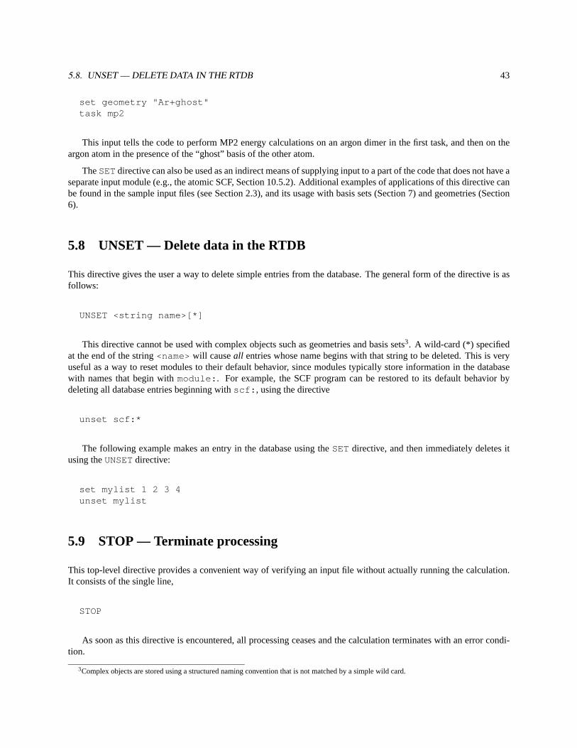
5.8. UNSET — DELETE DATA IN THE RTDB 43
set geometry "Ar+ghost"task mp2
This input tells the code to perform MP2 energy calculations on an argon dimer in the first task, and then on theargon atom in the presence of the “ghost” basis of the other atom.
TheSETdirective can also be used as an indirect means of supplying input to a part of the code that does not have aseparate input module (e.g., the atomic SCF, Section 10.5.2). Additional examples of applications of this directive canbe found in the sample input files (see Section 2.3), and its usage with basis sets (Section 7) and geometries (Section6).
5.8 UNSET — Delete data in the RTDB
This directive gives the user a way to delete simple entries from the database. The general form of the directive is asfollows:
UNSET <string name>[*]
This directive cannot be used with complex objects such as geometries and basis sets3. A wild-card (*) specifiedat the end of the string<name> will causeall entries whose name begins with that string to be deleted. This is veryuseful as a way to reset modules to their default behavior, since modules typically store information in the databasewith names that begin withmodule: . For example, the SCF program can be restored to its default behavior bydeleting all database entries beginning withscf: , using the directive
unset scf:*
The following example makes an entry in the database using theSET directive, and then immediately deletes itusing theUNSETdirective:
set mylist 1 2 3 4unset mylist
5.9 STOP — Terminate processing
This top-level directive provides a convenient way of verifying an input file without actually running the calculation.It consists of the single line,
STOP
As soon as this directive is encountered, all processing ceases and the calculation terminates with an error condi-tion.
3Complex objects are stored using a structured naming convention that is not matched by a simple wild card.
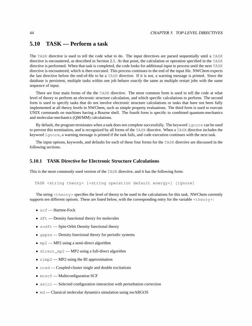
44 CHAPTER 5. TOP-LEVEL DIRECTIVES
5.10 TASK — Perform a task
The TASKdirective is used to tell the code what to do. The input directives are parsed sequentially until aTASKdirective is encountered, as described in Section 2.1. At that point, the calculation or operation specified in theTASKdirective is performed. When that task is completed, the code looks for additional input to process until the nextTASKdirective is encountered, which is then executed. This process continues to the end of the input file. NWChem expectsthe last directive before the end-of-file to be aTASKdirective. If it is not, a warning message is printed. Since thedatabase is persistent, multiple tasks within one job behaveexactlythe same as multiple restart jobs with the samesequence of input.
There are four main forms of the theTASKdirective. The most common form is used to tell the code at whatlevel of theory to perform an electronic structure calculation, and which specific calculations to perform. The secondform is used to specify tasks that do not involve electronic structure calculations or tasks that have not been fullyimplemented at all theory levels in NWChem, such as simple property evaluations. The third form is used to executeUNIX commands on machines having a Bourne shell. The fourth form is specific to combined quantum-mechanicsand molecular-mechanics (QM/MM) calculations.
By default, the program terminates when a task does not complete successfully. The keywordignore can be usedto prevent this termination, and is recognized by all forms of theTASKdirective. When aTASKdirective includes thekeywordignore , a warning message is printed if the task fails, and code execution continues with the next task.
The input options, keywords, and defaults for each of these four forms for theTASKdirective are discussed in thefollowing sections.
5.10.1 TASK Directive for Electronic Structure Calculations
This is the most commonly used version of theTASKdirective, and it has the following form:
TASK <string theory> [<string operation default energy>] [ignore]
The string<theory> specifies the level of theory to be used in the calculations for this task. NWChem currentlysupports ten different options. These are listed below, with the corresponding entry for the variable<theory> :
• scf — Hartree-Fock
• dft — Density functional theory for molecules
• sodft — Spin-Orbit Density functional theory
• gapss — Density functional theory for periodic systems
• mp2— MP2 using a semi-direct algorithm
• direct_mp2 — MP2 using a full-direct algorithm
• rimp2 — MP2 using the RI approximation
• ccsd — Coupled-cluster single and double excitations
• mcscf — Multiconfiguration SCF
• selci — Selected configuration interaction with perturbation correction
• md— Classical molecular dynamics simulation using nwARGOS
5.10. TASK — PERFORM A TASK 45
• cg\_pspw — Pseudopotential Plane-Wave DFT (PSPW)
The string<operation> specifies the calculation that will be performed in the task. The default operation is asingle point energy evaluation. The following list gives the selection of operations currently available in NWChem:
• energy — Evaluate the single point energy.
• gradient — Evaluate the derivative of the energy with respect to nuclear coordinates.
• optimize — Minimize the energy by varying the molecular structure. By default, this geometry optimizationis presently driven by the Driver module (see Section 19), but the Stepper module (see Section 20) may also beused.
• saddle — Conduct a search for a transition state (or saddle point) using either Driver (Section 19, the default)or Stepper (Section 20).
• frequencies or freq — Compute second derivatives and print out an analysis of molecular vibrations.
• dynamics — Compute molecular dynamics using nwARGOS.
• thermodynamics — Perform multi-configuration thermodynamic integration using nwARGOS.
The user should be aware that some of these operations (gradient, optimize, dynamics, thermodynamics) requirecomputation of derivatives of the energy with respect to the molecular coordinates. If analytical derivatives are notavailable (Section 4), they must be computed numerically, which can be very computationally intensive.
Here are some examples of theTASKdirective, to illustrate the input needed to specify particular calculations withthe code. To perform a single point energy evaluation using any level of theory, the directive is very simple, since theenergy evaluation is the default for the stringoperation . For an SCF energy calculation, the input line is simply
task scf
Equivalently, the operation can be specified explicitly, using the directive
task scf energy
Similarly, to perform a geometry optimization using density functional theory, theTASKdirective is
task dft optimize
The optional keywordignore can be used to allow execution to continue even if the task fails, as discussedabove.
5.10.2 TASK Directive for Special Operations
This form of theTASKdirective is used in instances where the task to be performed does not fit the model of theprevious version (such as execution of a Python program, Section 32), or if the operation has not yet been implementedin a fashion that applies to a wide range of theories (e.g., property evaluation). Instead of requiringtheory andoperation as input, the directive needs only a string identifying the task. The form of the directive in such cases isas follows:
TASK <string task> [ignore]
46 CHAPTER 5. TOP-LEVEL DIRECTIVES
The supported tasks that can be accessed with this form of theTASKdirective are listed below, with the corre-sponding entries for string variable<task> .
• python — Execute a Python program (Section 32).
• rtdbprint — Print the contents of the database.
• cphf — Invoke the CPHF module.
• property — Perform miscellaneous property calculations.
• dplot — Execute a DLOT run (Section 23)
• nbo — Execute a NBO run (Section 33.1)
This directive also recognizes the keywordignore , which allows execution to continue after a task has failed.
5.10.3 TASK Directive for the Bourne Shell
This form of theTASK directive is supported only on machines with a fully UNIX-style operating system. Thisdirective causes specified processes to be executed using the Bourne shell. This form of the task directive is:
TASK shell [(<integer-range process = 0>||all)] \<string command>
The keywordshell is required for this directive. It specifies that the given command will be executed in theBourne shell. The user can also specify which process(es) will execute this command by entering values forprocesson the directive. The default is for only process zero to execute the command. A range of processes may be specified,using Fortran triplet notation4. Alternatively, all processes can be specified simply by entering the keywordall . Theinput entered forcommand must form a single string, and must consist of valid UNIX command(s). If the stringincludes white space, it must be enclosed in double quotes.
For example, theTASK directive to tell process zero to copy the molecular orbitals file to a backup location/piofs/save can be input as follows:
task shell "cp *.movecs /piofs/save"
TheTASKdirective to tell all processes to list the contents of their/scratch directories is as follows:
task shell all "ls -l /scratch"
TheTASKdirective to tell processes 0 to 10 to remove the contents of the current directory is as follows:
task shell 0:10:1 "/bin/rm -f *"
Note that NWChem’s ability to quote special input characters isvery limited when compared with that of theBourne shell. To execute all but the simplest UNIX commands, it is usually much easier to put the shell script in a fileand execute the file from within NWChem.
4The notationlo:hi:inc denotes the integerslo , lo+inc , lo+2*inc , . . . ,hi
5.11. CHARGE — TOTAL SYSTEM CHARGE 47
5.10.4 TASK Directive for QM/MM simulations
This is very similar to the most commonly used version of theTASKdirective described in Section 5.10.1, and it hasthe following form;
TASK QMMM <string theory> [<string operation default energy>] [ignore]
The string<theory> specifies the QM theory to be used in the QM/MM simulation5. The level of theory may beany QM method that can compute gradients but those algorithms in NWChem that do not support analytic gradientsshould be avoided (c.f., Section 4).
The string<operation> is used to specify the calculation that will be performed in the QM/MM task. Thedefault operation is a single point energy evaluation. The following list gives the selection of operations currentlyavailable in the NWChem QM/MM module;
• energy — single point energy evaluation
• optimize — minimize the energy by variation of the molecular structure.
• dynamics — molecular dynamics using nwARGOS
Here are some examples of theTASKdirective for QM/MM simulations. To perform a single point energy of aQM/MM system using any QM level of theory, the directive is very simple. As with the general task directive, theQM/MM energy evaluation is the default. For a DFT energy calculation the task directive input is,
task qmmm dft
or completely as
task qmmm dft energy
To do a molecular dynamics simulation of a QM/MM system using the SCF level of theory the task directive inputwould be
task qmmm scf dynamics
The optional keywordignore can be used to allow execution to continue even if the task fails, as discussedabove.
5.11 CHARGE — Total system charge
This is an optional top-level directive that allows the user to specify the total charge of the system. The form of thedirective is as follows:
CHARGE <real charge default 0>
5If theory is “md” this is not a QM/MM simulation and will result in an appropriate error
48 CHAPTER 5. TOP-LEVEL DIRECTIVES
The default charge6 is zero if this directive is omitted. An example of a case where the directive would be neededis for a calculation on a doubly charged cation. In such a case, the directive is simply,
charge 2
If centers with fractional charge have been specified (Section 6) the net charge of the system should be adjusted toensure that there are an integral number of electrons.
The charge may be changed between tasks, and is used by all wavefunction types. For instance, in order tocompute the first two vertical ionization energies ofLiH , one might optimize the geometry ofLiH using a UHF SCFwavefunction, and then perform energy calculations at the optimized geometry onLiH + andLiH 2+ in turn. This isaccomplished with the following input:
geometry; Li 0 0 0; H 0 0 1.64; endbasis; Li library 3-21g; H library 3-21g; end
scf; uhf; singlet; endtask scf optimize
charge 1scf; uhf; doublet; endtask scf
charge 2scf; uhf; singlet; endtask scf
TheGEOMETRY, BASIS, andSCFdirectives are described below (Sections 6, 7 and 10 respectively) but their intentshould be clear. TheTASKdirective is described above (Section 5.10).
6The charge directive, in conjunction with the charges of atomic nuclei (which can be changed via the geometry input, cf. Section 6.3),determines the total number of electrons in the chemical system. Therefore, acharge n specification removes "n" electrons from the chemicalsystem. Similarly,charge -n adds "n" electrons.
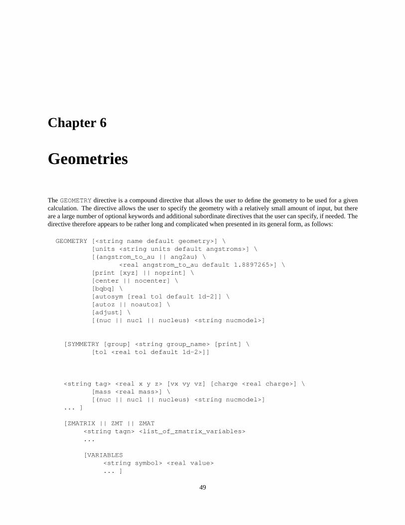
Chapter 6
Geometries
TheGEOMETRYdirective is a compound directive that allows the user to define the geometry to be used for a givencalculation. The directive allows the user to specify the geometry with a relatively small amount of input, but thereare a large number of optional keywords and additional subordinate directives that the user can specify, if needed. Thedirective therefore appears to be rather long and complicated when presented in its general form, as follows:
GEOMETRY [<string name default geometry>] \[units <string units default angstroms>] \[(angstrom_to_au || ang2au) \
<real angstrom_to_au default 1.8897265>] \[print [xyz] || noprint] \[center || nocenter] \[bqbq] \[autosym [real tol default 1d-2]] \[autoz || noautoz] \[adjust] \[(nuc || nucl || nucleus) <string nucmodel>]
[SYMMETRY [group] <string group_name> [print] \[tol <real tol default 1d-2>]]
<string tag> <real x y z> [vx vy vz] [charge <real charge>] \[mass <real mass>] \[(nuc || nucl || nucleus) <string nucmodel>]
... ]
[ZMATRIX || ZMT || ZMAT<string tagn> <list_of_zmatrix_variables>...
[VARIABLES<string symbol> <real value>... ]
49
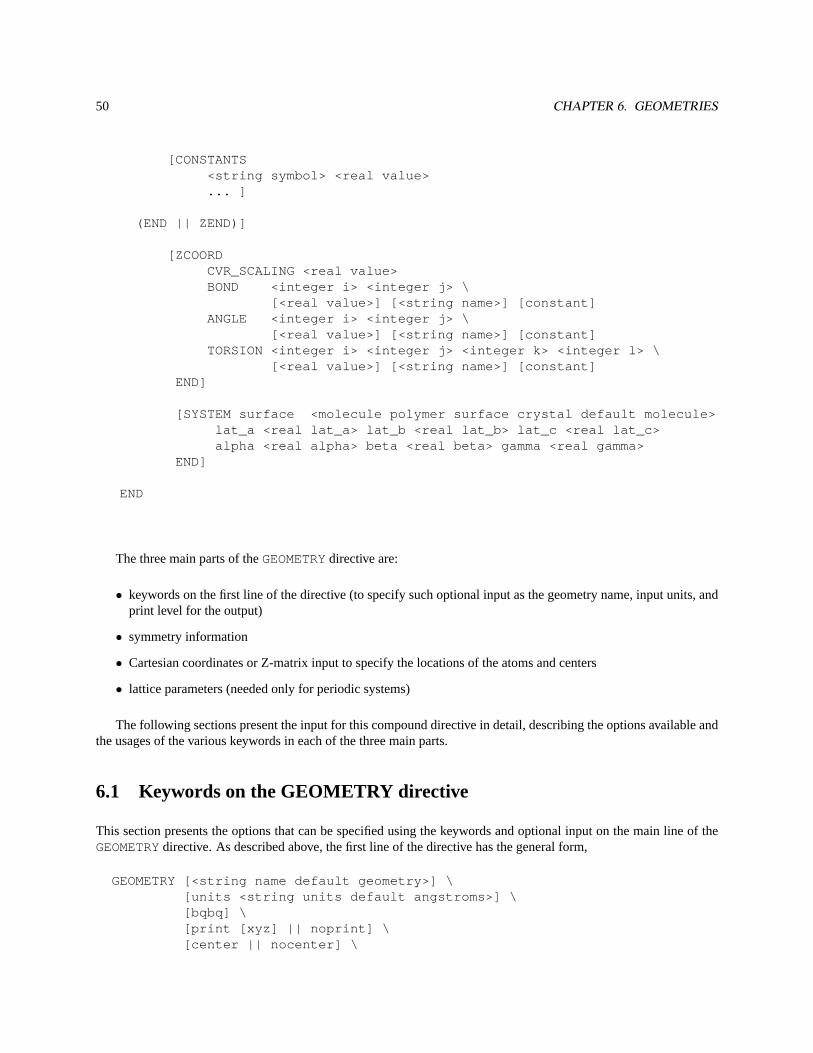
50 CHAPTER 6. GEOMETRIES
[CONSTANTS<string symbol> <real value>... ]
(END || ZEND)]
[ZCOORDCVR_SCALING <real value>BOND <integer i> <integer j> \
[<real value>] [<string name>] [constant]ANGLE <integer i> <integer j> \
[<real value>] [<string name>] [constant]TORSION <integer i> <integer j> <integer k> <integer l> \
[<real value>] [<string name>] [constant]END]
[SYSTEM surface <molecule polymer surface crystal default molecule>lat_a <real lat_a> lat_b <real lat_b> lat_c <real lat_c>alpha <real alpha> beta <real beta> gamma <real gamma>
END]
END
The three main parts of theGEOMETRYdirective are:
• keywords on the first line of the directive (to specify such optional input as the geometry name, input units, andprint level for the output)
• symmetry information
• Cartesian coordinates or Z-matrix input to specify the locations of the atoms and centers
• lattice parameters (needed only for periodic systems)
The following sections present the input for this compound directive in detail, describing the options available andthe usages of the various keywords in each of the three main parts.
6.1 Keywords on the GEOMETRY directive
This section presents the options that can be specified using the keywords and optional input on the main line of theGEOMETRYdirective. As described above, the first line of the directive has the general form,
GEOMETRY [<string name default geometry>] \[units <string units default angstroms>] \[bqbq] \[print [xyz] || noprint] \[center || nocenter] \
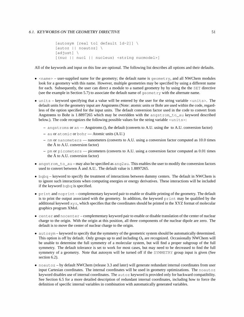
6.1. KEYWORDS ON THE GEOMETRY DIRECTIVE 51
[autosym [real tol default 1d-2]] \[autoz || noautoz] \[adjust] \[(nuc || nucl || nucleus) <string nucmodel>]
All of the keywords and input on this line are optional. The following list describes all options and their defaults.
• <name> – user-supplied name for the geometry; the default name isgeometry , and all NWChem moduleslook for a geometry with this name. However, multiple geometries may be specified by using a different namefor each. Subsequently, the user can direct a module to a named geometry by by using the theSET directive(see the example in Section 5.7) to associate the default name ofgeometry with the alternate name.
• units – keyword specifying that a value will be entered by the user for the string variable<units> . Thedefault units for the geometry input are Angstrøms (Note: atomic units or Bohr are used within the code, regard-less of the option specified for the input units. The default conversion factor used in the code to convert fromAngstrøms to Bohr is 1.8897265 which may be overidden with theangstrom_to_au keyword describedbelow.). The code recognizes the following possible values for the string variable<units> :
– angstroms or an — Angstroms (), the default (converts to A.U. using the to A.U. conversion factor)
– au or atomic or bohr — Atomic units (A.U.)
– nmor nanometers — nanometers (converts to A.U. using a conversion factor computed as 10.0 timesthe Å to A.U. conversion factor)
– pmor picometers — picometers (converts to A.U. using a conversion factor computed as 0.01 timesthe Å to A.U. conversion factor)
• angstrom_to_au – may also be specified asang2au . This enables the user to modify the conversion factorsused to convert between Å and A.U.. The default value is 1.8897265.
• bqbq – keyword to specify the treatment of interactions between dummy centers. The default in NWChem isto ignore such interactions when computing energies or energy derivatives. These interactions will be includedif the keywordbqbq is specified.
• print andnoprint – complementary keyword pair to enable or disable printing of the geometry. The defaultis to print the output associated with the geometry. In addition, the keywordprint may be qualified by theadditional keywordxyz , which specifies that the coordinates should be printed in the XYZ format of moleculargraphics program XMol.
• center andnocenter – complementary keyword pair to enable or disable translation of the center of nuclearcharge to the origin. With the origin at this position, all three components of the nuclear dipole are zero. Thedefault is to move the center of nuclear charge to the origin.
• autosym – keyword to specify that the symmetry of the geometric system should be automatically determined.This option is off by default. Only groups up to and includingOh are recognized. Occasionally NWChem willbe unable to determine the full symmetry of a molecular system, but will find a proper subgroup of the fullsymmetry. The default tolerance is set to work for most cases, but may need to be decreased to find the fullsymmetry of a geometry. Note that autosym will be turned off if theSYMMETRYgroup input is given (Seesection 6.2).
• noautoz – by default NWChem (release 3.3 and later) will generate redundant internal coordinates from userinput Cartesian coordinates. The internal coordinates will be used in geometry optimizations. Thenoautozkeyword disables use of internal coordinates. Theautoz keyword is provided only for backward compatibility.See Section 6.5 for a more detailed description of redundant internal coordinates, including how to force thedefinition of specific internal variables in combination with automatically generated variables.
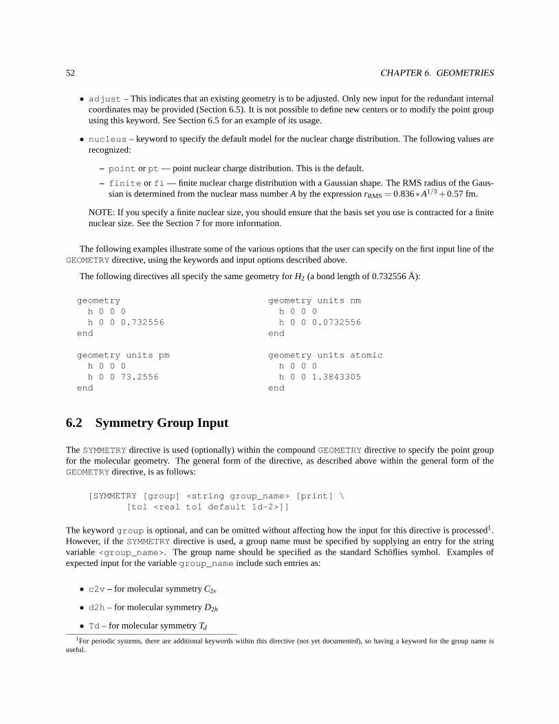
52 CHAPTER 6. GEOMETRIES
• adjust – This indicates that an existing geometry is to be adjusted. Only new input for the redundant internalcoordinates may be provided (Section 6.5). It is not possible to define new centers or to modify the point groupusing this keyword. See Section 6.5 for an example of its usage.
• nucleus – keyword to specify the default model for the nuclear charge distribution. The following values arerecognized:
– point or pt — point nuclear charge distribution. This is the default.
– finite or fi — finite nuclear charge distribution with a Gaussian shape. The RMS radius of the Gaus-sian is determined from the nuclear mass numberA by the expressionrRMS = 0.836∗A1/3 +0.57 fm.
NOTE: If you specify a finite nuclear size, you should ensure that the basis set you use is contracted for a finitenuclear size. See the Section 7 for more information.
The following examples illustrate some of the various options that the user can specify on the first input line of theGEOMETRYdirective, using the keywords and input options described above.
The following directives all specify the same geometry forH2 (a bond length of 0.732556 Å):
geometry geometry units nmh 0 0 0 h 0 0 0h 0 0 0.732556 h 0 0 0.0732556
end end
geometry units pm geometry units atomich 0 0 0 h 0 0 0h 0 0 73.2556 h 0 0 1.3843305
end end
6.2 Symmetry Group Input
TheSYMMETRYdirective is used (optionally) within the compoundGEOMETRYdirective to specify the point groupfor the molecular geometry. The general form of the directive, as described above within the general form of theGEOMETRYdirective, is as follows:
[SYMMETRY [group] <string group_name> [print] \[tol <real tol default 1d-2>]]
The keywordgroup is optional, and can be omitted without affecting how the input for this directive is processed1.However, if theSYMMETRYdirective is used, a group name must be specified by supplying an entry for the stringvariable<group_name> . The group name should be specified as the standard Schöflies symbol. Examples ofexpected input for the variablegroup_name include such entries as:
• c2v – for molecular symmetryC2v
• d2h – for molecular symmetryD2h
• Td – for molecular symmetryTd
1For periodic systems, there are additional keywords within this directive (not yet documented), so having a keyword for the group name isuseful.
6.3. CARTESIAN COORDINATE INPUT 53
• d6h – for molecular symmetryD6h
TheSYMMETRYdirective is optional. The default is no symmetry (i.e.,C1 point group). Automatic detection ofpoint group symmetry is available through the use ofautosym in theGEOMETRYdirective main line (discussed inSection 6.1). Note: if theSYMMETRYdirective is present theautosym keyword is ignored.
If only symmetry-unique atoms are specified, the others will be generated through the action of the point groupoperators, but the user if free to specify all atoms. The user must know the symmetry of the molecule being modeled,and be able to specify the coordinates of the atoms in a suitable orientation relative to the rotation axes and planes ofsymmetry. Appendix C lists a number of examples of theGEOMETRYdirective input for specific molecules havingsymmetry patterns recognized by NWChem. The exact point group symmetry will be forced upon the molecule, andatoms within 10−3 A.U. of a symmetry element (e.g., a mirror plane or rotation axis) will be forced onto that element.Thus, it is not necessary to specify to a high precision those coordinates that are determined solely by symmetry.
The keywordprint gives information concerning the point group generation, including the group generators, acharacter table, the mapping of centers, and the group operations.
The keywordtol relates to the accuracy with which the symmetry-unique atoms should be specified. When theatoms are generated, those that are within the tolerance,tol , are considered the same.
6.3 Cartesian coordinate input
The default in NWChem is to specify the geometry information entirely in Cartesian coordinates, and examples of thisformat have appeared above (e.g, Section 2.3). Each center (usually an atom) is identified on a line of the followingform:
<string tag> <real x y z> [vx vy vz] \[charge <real charge>] [mass <real mass>] \[(nuc || nucl || nucleus) <string nucmodel>]
The string<tag> is the name of the atom or center, and its case (upper or lower) is important. The tag is limitedto 16 characters and is interpreted as follows:
• If the entry for <tag> begins with either the symbol or name of an element (regardless of case), then thecenter is treated as an atom of that type. The default charge is the atomic number (adjusted for the presenceof ECPs by the ECPNELECdirective ; see Section 8). Additional characters can be added to the string, todistinguish between atoms of the same element (For example, the tagsoxygen , O, o34 , olonepair , andOxygen-ether , will all be interpreted as oxygen atoms.).
• If the entry for<tag> begins with the charactersbq or x (regardless of case), then the center is treated as adummy center with a default zero charge (Note: a tag beginning with the charactersxe will be interpreted as axenon atom rather than as a dummy center.). Dummy centers may optionally have basis functions or non-zerocharge. See Section B.2 for a sample input using dummy centers with charges.
It is importantto be aware of the following points regarding the definitions and usage of the values specified forthe variable<tag> to describe the centers in a system:
• If the tag begins with characters that cannot be matched against an atom, and those characters are notBQor X,then a fatal error is generated.
54 CHAPTER 6. GEOMETRIES
• The tag of a center is used in theBASIS (Section 7) andECP(Section 8) directives to associate functions withcenters.
• All centers with the same tag will have the same basis functions.
• When using automatic symmetry detection, only centers with the same tag will be candidates for testing forsymmetry equivalence.
• The user-specified charges (of all centers, atomic and dummy) and any net total charge of the system (Section5.11) are used to determine the number of electrons in the system.
The Cartesian coordinates of the atom in the molecule are specified as real numbers supplied for the variablesx ,y , andz following the characters entered for the tag. The values supplied for the coordinates must be in the unitsspecified by the value of the variable<units> on the first line of theGEOMETRYdirective input.
After the Cartesian coordinate input, optional velocities may be entered as real numbers for the variablesvx , vy ,andvz . The velocities should be given in atomic units and are used in QMD and PSPW calculations.
The Cartesian coordinate input line also contains the optional keywordscharge , mass andnucleus , whichallow the user to specify the charge of the atom (or center) and its mass (in atomic mass units), and the nuclear model.The default charge for an atom is its atomic number, adjusted for the presence of ECPs (see Section 8). In order tospecify a different value for the charge on a particular atom, the user must enter the keywordcharge , followed bythe desired value for the variable<charge> .
The default mass for an atom is taken to be the mass of its most abundant naturally occurring isotope or of theisotope with the longest half-life. To model some other isotope of the element, its mass must be defined explicitly byspecifying the keywordmass, followed by the value (in atomic mass units) for the variable<mass>.
The default nuclear model is a point nucleus. The keywordnucleus (or nucl or nuc ) followed by the modelname<nucmodel> overrides this default. Allowed values of<nucmodel> arepoint or pt andfinite or fi .Thefinite option is a nuclear model with a Gaussian shape. The RMS radius of the Gaussian is determined by theatomic mass number via the formularRMS = 0.836∗A1/3 + 0.57 fm. The mass numberA is derived from the variable<mass>.
The geometry of the system can be specified entirely in Cartesian coordinates by supplying a<tag> line of thetype described above for each atom or center. The user has the option, however, of supplying the geometry of some orall of the atoms or centers using a Z-matrix description. In such a case, the user supplies the input tag line describedabove for any centers to be described by Cartesian coordinates, and then specifies the remainder of the system usingthe optionalZMATRIXdirective described below in Section 6.4.
6.4 Z-matrix input
TheZMATRIXdirective is an optional directive that can be used within the compoundGEOMETRYdirective to specifythe structure of the system with a Z-matrix, which can include both internal and Cartesian coordinates. TheZMATRIXdirective is itself a compound directive that can include theVARIABLESandCONSTANTSdirectives, depending onthe options selected. The general form of the compoundZMATRIXdirective is as follows:
[ZMATRIX || ZMT || ZMAT<string tagn> <list_of_zmatrix_variables>...
[VARIABLES<string symbol> <real value>
6.4. Z-MATRIX INPUT 55
... ]
[CONSTANTS<string symbol> <real value>... ]
(END || ZEND)]
The input module recognizes three possible spellings of this directive name. It can be invoked withZMATRIX,ZMT, or ZMAT. The user can specify the molecular structure using either Cartesian coordinates or internal coordinates(bond lengths, bond angles and dihedral angles. The Z-matrix input for a center defines connectivity, bond length,and bond or torsion angles. Cartesian coordinate input for a center consists of three real numbers defining the x,y,zcoordinates of the atom.
Within the Z-matrix input, bond lengths and Cartesian coordinates must be input in the user-specified units, asdefined by the value specified for the variable<units> on the first line of theGEOMETRYdirective. All angles arespecified in degrees.
The individual centers (denoted asi , j , andk below) used to specify Z-matrix connectivity may be designatedeither as integers (identifying each center by number) or as tags (If tags are used, the tag must be unique for eachcenter.) The use of “dummy” atoms is possible, by usingX or BQat the start of the tag.
Bond lengths, bond angles and dihedral angles (denoted below asR, alpha , andbeta , respectively) may bespecified either as numerical values or as symbolic strings that must be subsequently defined using theVARIABLESorCONSTANTSdirectives. The numerical values of the symbolic strings labeledVARIABLESmay be subject to changesduring a geometry optimization say, while the numerical values of the symbolic strings labeled |verb+CONSTANTS+will stay frozen to the value given in the input. The same symbolic string can be used more than once, and any mixtureof numeric data and symbols is acceptable. Bond angles (α) must be in the range 0< α< 180.
The Z-matrix input is specified sequentially as follows:
tag1tag2 i Rtag3 i R j alphatag4 i R j alpha k beta [orient]...
The structure of this input is described in more detail below. In the following discussion, the tag or number of thecenter being currently defined is labeled asC (“C” for current). The values entered for these tags for centers defined inthe Z-matrix input are interpreted in the same way as the<tag> entries for Cartesian coordinates described above (seeSection 6.3). Figures 6.1, 6.2 and 6.3 display the relationships between the input data and the definitions of centersand angles.
The Z-matrix input shown above is interpreted as follows:
1. tag1
Only a tag is required for the first center.
2. tag2 i R
The second center requires specification of its tag and the bond length (RCi) distance to a previous atom, whichis identified byi .
3. tag3 i R j alpha
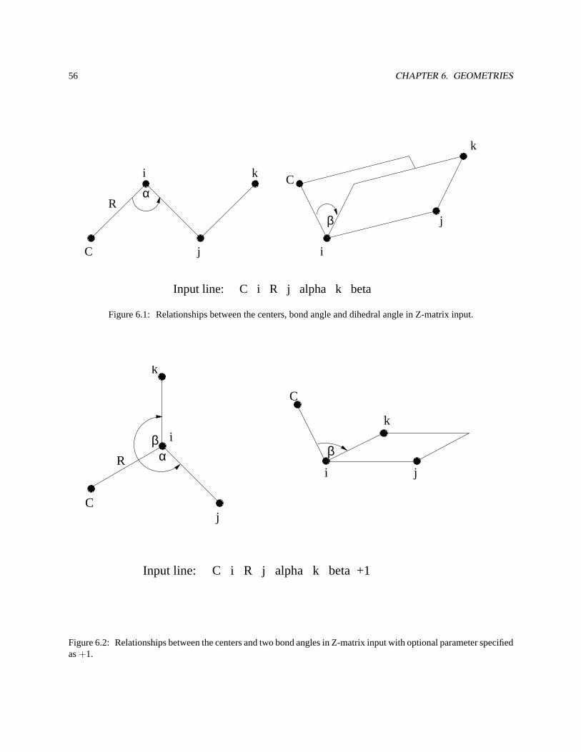
56 CHAPTER 6. GEOMETRIES
��������
����
����
����
����
i
α
j
k
C��������
��������
��������R
β
C
i
j
k
Input line: C i R j alpha k beta
Figure 6.1: Relationships between the centers, bond angle and dihedral angle in Z-matrix input.
������������
������
��������
����
��������
������������
��������
i
k
β
��������Cj
αRj
k
C
i
β
Input line: C i R j alpha k beta +1
Figure 6.2: Relationships between the centers and two bond angles in Z-matrix input with optional parameter specifiedas+1.
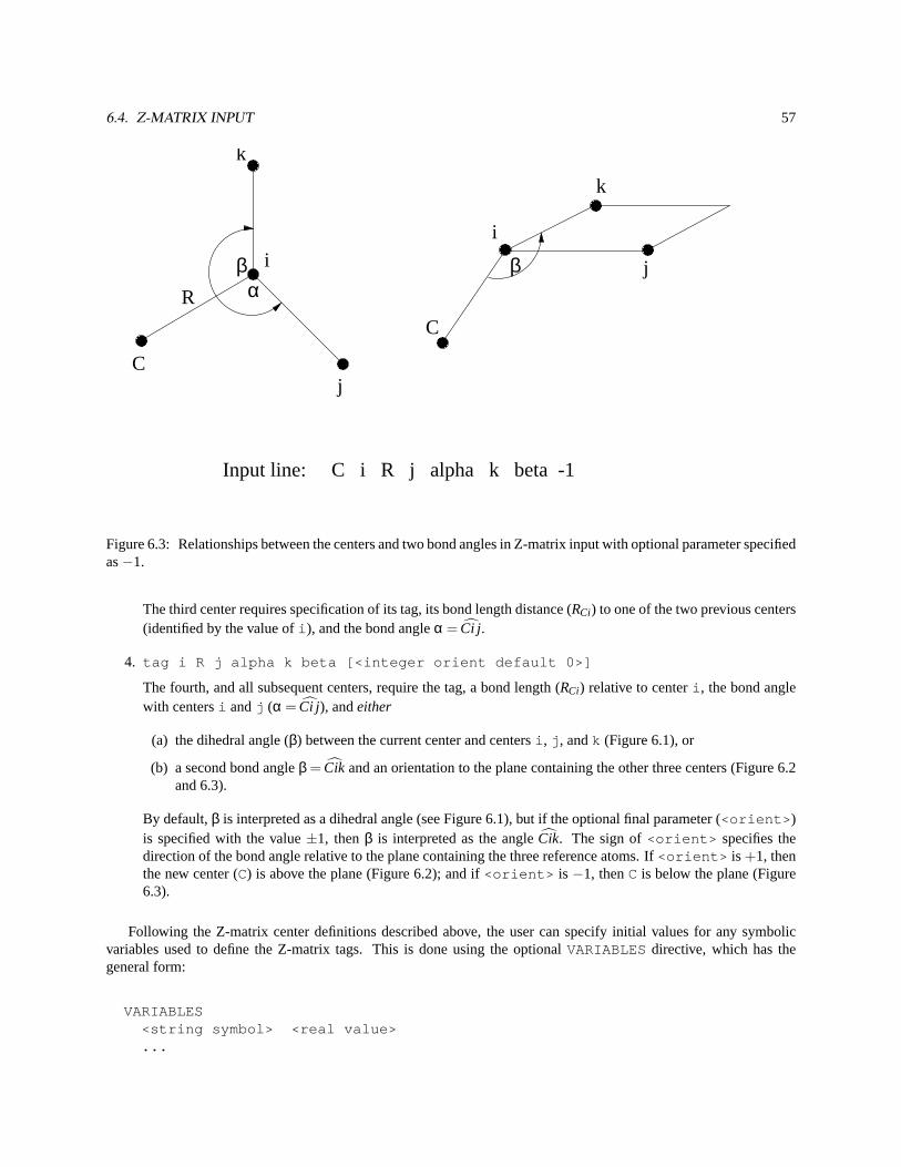
6.4. Z-MATRIX INPUT 57
������������
������������
��������
����
��������
������������
��������
i
k
β
��������Cj
αR
j
k
i
β
C
Input line: C i R j alpha k beta -1
Figure 6.3: Relationships between the centers and two bond angles in Z-matrix input with optional parameter specifiedas−1.
The third center requires specification of its tag, its bond length distance (RCi) to one of the two previous centers(identified by the value ofi ), and the bond angleα = Ci j.
4. tag i R j alpha k beta [<integer orient default 0>]
The fourth, and all subsequent centers, require the tag, a bond length (RCi) relative to centeri , the bond anglewith centersi andj (α = Ci j), andeither
(a) the dihedral angle (β) between the current center and centersi , j , andk (Figure 6.1), or
(b) a second bond angleβ = Cik and an orientation to the plane containing the other three centers (Figure 6.2and 6.3).
By default,β is interpreted as a dihedral angle (see Figure 6.1), but if the optional final parameter (<orient> )is specified with the value±1, thenβ is interpreted as the angleCik. The sign of<orient> specifies thedirection of the bond angle relative to the plane containing the three reference atoms. If<orient> is +1, thenthe new center (C) is above the plane (Figure 6.2); and if<orient> is−1, thenC is below the plane (Figure6.3).
Following the Z-matrix center definitions described above, the user can specify initial values for any symbolicvariables used to define the Z-matrix tags. This is done using the optionalVARIABLES directive, which has thegeneral form:
VARIABLES<string symbol> <real value>...
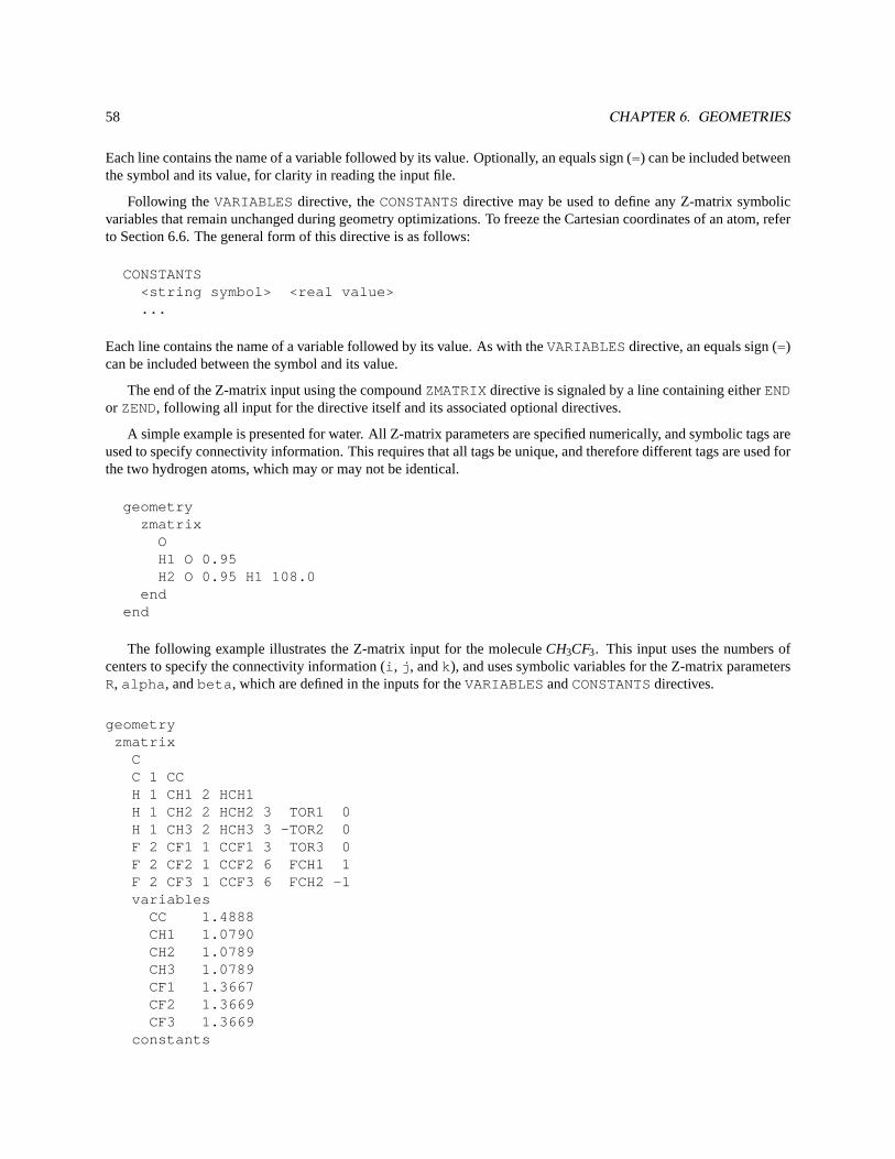
58 CHAPTER 6. GEOMETRIES
Each line contains the name of a variable followed by its value. Optionally, an equals sign (=) can be included betweenthe symbol and its value, for clarity in reading the input file.
Following theVARIABLES directive, theCONSTANTSdirective may be used to define any Z-matrix symbolicvariables that remain unchanged during geometry optimizations. To freeze the Cartesian coordinates of an atom, referto Section 6.6. The general form of this directive is as follows:
CONSTANTS<string symbol> <real value>...
Each line contains the name of a variable followed by its value. As with theVARIABLESdirective, an equals sign (=)can be included between the symbol and its value.
The end of the Z-matrix input using the compoundZMATRIXdirective is signaled by a line containing eitherENDor ZEND, following all input for the directive itself and its associated optional directives.
A simple example is presented for water. All Z-matrix parameters are specified numerically, and symbolic tags areused to specify connectivity information. This requires that all tags be unique, and therefore different tags are used forthe two hydrogen atoms, which may or may not be identical.
geometryzmatrix
OH1 O 0.95H2 O 0.95 H1 108.0
endend
The following example illustrates the Z-matrix input for the moleculeCH3CF3. This input uses the numbers ofcenters to specify the connectivity information (i , j , andk ), and uses symbolic variables for the Z-matrix parametersR, alpha , andbeta , which are defined in the inputs for theVARIABLESandCONSTANTSdirectives.
geometryzmatrix
CC 1 CCH 1 CH1 2 HCH1H 1 CH2 2 HCH2 3 TOR1 0H 1 CH3 2 HCH3 3 -TOR2 0F 2 CF1 1 CCF1 3 TOR3 0F 2 CF2 1 CCF2 6 FCH1 1F 2 CF3 1 CCF3 6 FCH2 -1variables
CC 1.4888CH1 1.0790CH2 1.0789CH3 1.0789CF1 1.3667CF2 1.3669CF3 1.3669
constants
6.5. ZCOORD — FORCING INTERNAL COORDINATES 59
HCH1 104.28HCH2 104.74HCH3 104.7CCF1 112.0713CCF2 112.0341CCF3 112.0340TOR1 109.3996TOR2 109.3997TOR3 180.0000FCH1 106.7846FCH2 106.7842
endend
The input for any centers specified with Cartesian coordinates must be specified using the format of the<tag>lines described in Section 6.3 above. However, in order to correctly specify these Cartesian coordinates within theZ-matrix, the user must understand the orientation of centers specified using internal coordinates. These are arrangedas follows:
• The first center is placed at the origin.
• The second center is placed along the positive z-axis.
• The third center is placed in the z-x plane.
6.5 ZCOORD — Forcing internal coordinates
By default redundant internal coordinates are generated for use in geometry optimizations. Connectivity is inferredby comparing inter-atomic distances with the sum of the van der Waals radii of the two atoms involved in a possiblebond, times a scaling factor. The scaling factor is an input parameter ofZCOORDwhich maybe changed from its defaultvalue of 1.3. Under some circumstances (unusual bonding, bond dissociation, . . . ) it will be necessary to augmentthe automatically generated list of internal coordinates to force some specific internal coordinates to be included inamong the internal coordinates. This is accomplished by including the optional directiveZCOORDwithin the geometrydirective. The general form of theZCOORDdirective is as follows:
ZCOORDCVR_SCALING <real value>BOND <integer i> <integer j> \
[<real value>] [<string name>] [constant]ANGLE <integer i> <integer j> <integer k> \
[<real value>] [<string name>] [constant]TORSION <integer i> <integer j> <integer k> <integer l> \
[<real value>] [<string name>] [constant]END
The centersi , j , k and l mustbe specified using the numbers of the centers, as supplied in the input for theCartesian coordinates. TheZCOORDinput parameters are defined as follows:
• cvr_scaling — scaling factor applied to van der Waals radii.
60 CHAPTER 6. GEOMETRIES
• bond — a bond between the two centers.
• angle — a bond anglei jk.
• torsion — a torsion (or dihedral) angle. The angle between the planesi-j-k andj-k-l .
A value may be specified for a user-defined internal coordinate, in which case it is forced upon the input Cartesiancoordinates while attempting to make only small changes in the other internal coordinates. If no value is provided thevalue implicit in the input coordinates is kept. If the keywordconstant is specified, then that internal variable is notmodified during a geometry optimization with DRIVER (Section 19). Each internal coordinate may also be namedeither for easy identification in the output, or for the application of constraints (Section 6.6).
If the keywordadjust is specified on the mainGEOMETRYdirective, onlyZCOORDdata may be specified and itcan be used to change the user-defined internal coordinates, including adding/removing constraints and changing theirvalues.
6.6 Applying constraints in geometry optimizations
Internal coordinates specified as constant in aZCOORDdirective or in the constants section of aZMATRIXdirective,will be frozen at their initial values if a geometry optimization is performed with DRIVER (Section 19).
If internal coordinates have the same name (give or take an optional sign for torsions) then they are forced to havethe same value. This may be used to force bonds or angles to be equal even if they are not related by symmetry.
When atoms have been specified by their cartesian coordinates,and internal coordinates are not being used, it ispossible to freeze the cartesian position of selected atoms. This is useful for such purposes as optimizing a moleculeabsorbed on the surface of a cluster with fixed geometry. Only the gradients associated with the active atoms arecomputed. This can result in a big computational saving, since gradients associated with frozen atoms are forced tozero (Note, however, that this destroys the translational and rotational invariance of the gradient. This is not yet fullyaccommodated by the STEPPER geometry optimization software, and can sometimes result in slower convergence ofthe optimization. The DRIVER optimization package does not suffer from this problem).
TheSETdirective (Section 5.7) is used to freeze atoms, by specifying a directive of the form:
set geometry:actlist <integer list_of_center_numbers>
This defines only the centers in the list as active. All other centers will have zero force assigned to them, and willremain frozen at their starting coordinates during a geometry optimization.
For example, the following directive specifies that atoms numbered 1, 5, 6, 7, 8, and 15 are active and all otheratoms are frozen:
set geometry:actlist 1 5:8 15
or equivalently,
set geometry:actlist 1 5 6 7 8 15
If this option is not specified by entering aSET directive, the default behavior in the code is to treat all atoms asactive. To revert to this default behavior after the option to define frozen atoms has been invoked, theUNSETdirectivemust be used (since the database is persistent, see Section 3.2). The form of theUNSETdirective is as follows:
unset geometry:actlist
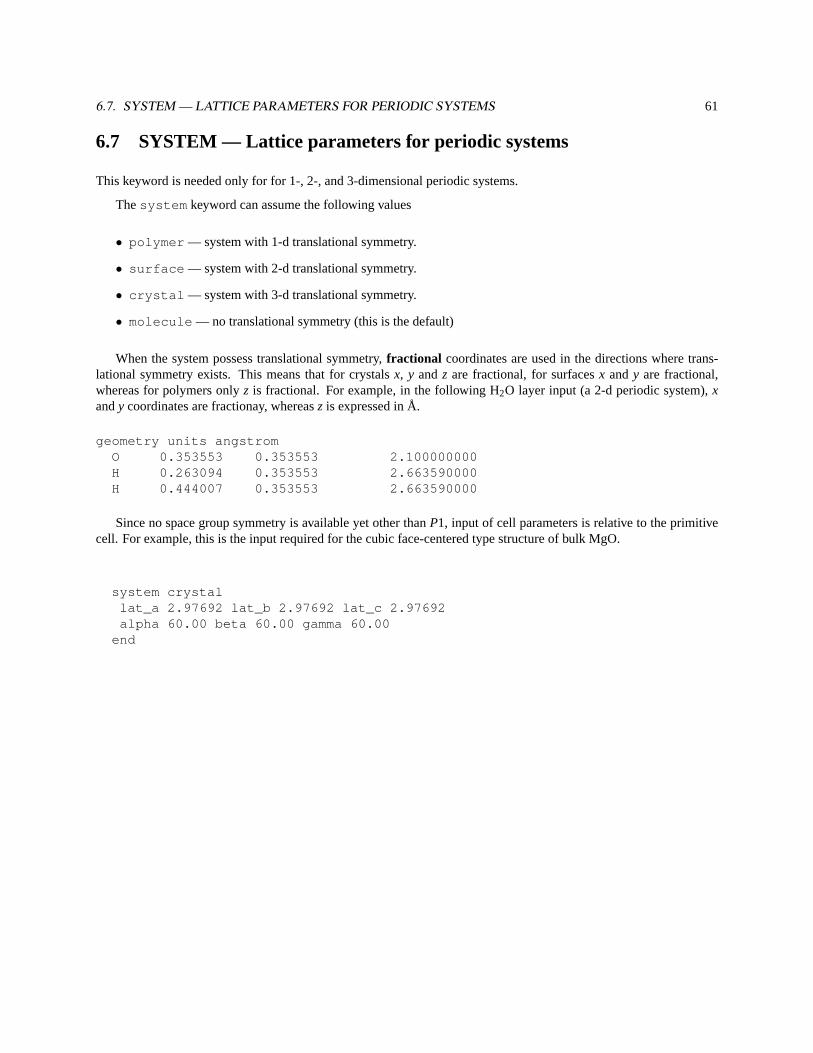
6.7. SYSTEM — LATTICE PARAMETERS FOR PERIODIC SYSTEMS 61
6.7 SYSTEM — Lattice parameters for periodic systems
This keyword is needed only for for 1-, 2-, and 3-dimensional periodic systems.
Thesystem keyword can assume the following values
• polymer — system with 1-d translational symmetry.
• surface — system with 2-d translational symmetry.
• crystal — system with 3-d translational symmetry.
• molecule — no translational symmetry (this is the default)
When the system possess translational symmetry,fractional coordinates are used in the directions where trans-lational symmetry exists. This means that for crystalsx, y andz are fractional, for surfacesx andy are fractional,whereas for polymers onlyz is fractional. For example, in the following H2O layer input (a 2-d periodic system),xandy coordinates are fractionay, whereasz is expressed in Å.
geometry units angstromO 0.353553 0.353553 2.100000000H 0.263094 0.353553 2.663590000H 0.444007 0.353553 2.663590000
Since no space group symmetry is available yet other thanP1, input of cell parameters is relative to the primitivecell. For example, this is the input required for the cubic face-centered type structure of bulk MgO.
system crystallat_a 2.97692 lat_b 2.97692 lat_c 2.97692alpha 60.00 beta 60.00 gamma 60.00
end

62 CHAPTER 6. GEOMETRIES
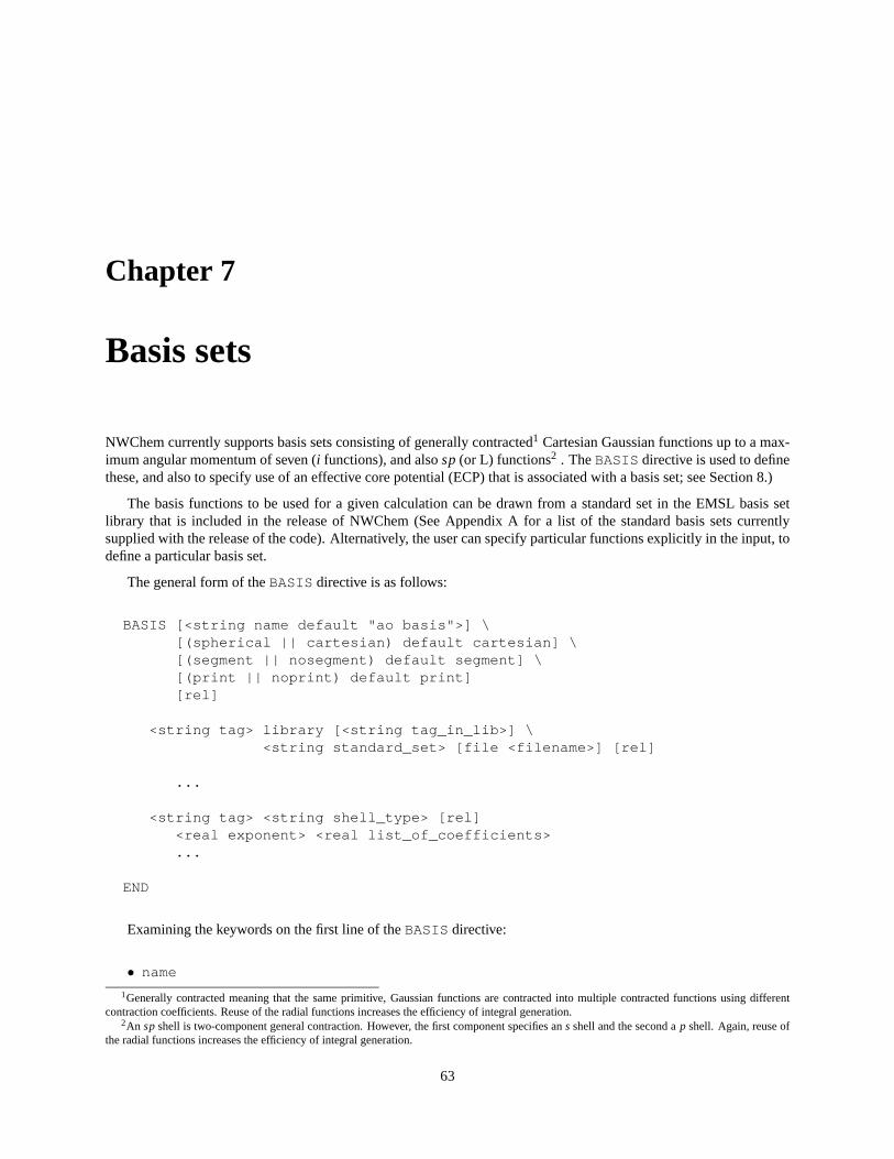
Chapter 7
Basis sets
NWChem currently supports basis sets consisting of generally contracted1 Cartesian Gaussian functions up to a max-imum angular momentum of seven (i functions), and alsosp(or L) functions2 . TheBASIS directive is used to definethese, and also to specify use of an effective core potential (ECP) that is associated with a basis set; see Section 8.)
The basis functions to be used for a given calculation can be drawn from a standard set in the EMSL basis setlibrary that is included in the release of NWChem (See Appendix A for a list of the standard basis sets currentlysupplied with the release of the code). Alternatively, the user can specify particular functions explicitly in the input, todefine a particular basis set.
The general form of theBASIS directive is as follows:
BASIS [<string name default "ao basis">] \[(spherical || cartesian) default cartesian] \[(segment || nosegment) default segment] \[(print || noprint) default print][rel]
<string tag> library [<string tag_in_lib>] \<string standard_set> [file <filename>] [rel]
...
<string tag> <string shell_type> [rel]<real exponent> <real list_of_coefficients>...
END
Examining the keywords on the first line of theBASIS directive:
• name
1Generally contracted meaning that the same primitive, Gaussian functions are contracted into multiple contracted functions using differentcontraction coefficients. Reuse of the radial functions increases the efficiency of integral generation.
2An spshell is two-component general contraction. However, the first component specifies ans shell and the second ap shell. Again, reuse ofthe radial functions increases the efficiency of integral generation.
63
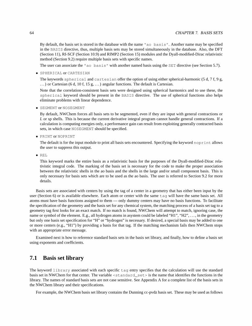
64 CHAPTER 7. BASIS SETS
By default, the basis set is stored in the database with the name"ao basis" . Another name may be specifiedin theBASIS directive, thus, multiple basis sets may be stored simultaneously in the database. Also, the DFT(Section 11), RI-SCF (Section 10.9) and RIMP2 (Section 15) modules and the Dyall-modified-Dirac relativisticmethod (Section 9.2) require multiple basis sets with specific names.
The user can associate the"ao basis" with another named basis using theSETdirective (see Section 5.7).
• SPHERICALor CARTESIAN
The keywordsspherical andcartesian offer the option of using either spherical-harmonic (5 d, 7 f, 9 g,. . . ) or Cartesian (6 d, 10 f, 15 g, . . . ) angular functions. The default is Cartesian.
Note that the correlation-consistent basis sets were designed using spherical harmonics and to use these, thespherical keyword should be present in theBASIS directive. The use of spherical functions also helpseliminate problems with linear dependence.
• SEGMENTor NOSEGMENT
By default, NWChem forces all basis sets to be segmented, even if they are input with general contractions orL or sp shells. This is because the current derivative integral program cannot handle general contractions. If acalculation is computing energies only, a performance gain can result from exploiting generally contracted basissets, in which caseNOSEGMENTshould be specified.
• PRINT or NOPRINT
The default is for the input module to print all basis sets encountered. Specifying the keywordnoprint allowsthe user to suppress this output.
• REL
This keyword marks the entire basis as a relativistic basis for the purposes of the Dyall-modified-Dirac rela-tivistic integral code. The marking of the basis set is necessary for the code to make the proper associationbetween the relativistic shells in the ao basis and the shells in the large and/or small component basis. This isonly necessary for basis sets which are to be used as the ao basis. The user is referred to Section 9.2 for moredetails.
Basis sets are associated with centers by using the tag of a center in a geometry that has either been input by theuser (Section 6) or is available elsewhere. Each atom or center with the sametag will have the same basis set. Allatoms must have basis functions assigned to them — only dummy centers may have no basis functions. To facilitatethe specification of the geometry and the basis set for any chemical system, the matching process of a basis set tag to ageometry tag first looks for an exact match. If no match is found, NWChem will attempt to match, ignoring case, thename or symbol of the element. E.g., all hydrogen atoms in asystem could be labeled “H1”, “H2”, . . . , in the geometrybut only one basis set specification for “H” or “hydrogen” is necessary. If desired, a special basis may be added to oneor more centers (e.g., “H1”) by providing a basis for that tag. If the matching mechanism fails then NWChem stopswith an appropriate error message.
Examined next is how to reference standard basis sets in the basis set library, and finally, how to define a basis setusing exponents and coefficients.
7.1 Basis set library
The keywordlibrary associated with each specifictag entry specifies that the calculation will use the standardbasis set in NWChem for that center. The variable<standard_set> is the name that identifies the functions in thelibrary. The names of standard basis sets are not case sensitive. See Appendix A for a complete list of the basis sets inthe NWChem library and their specifications.
For example, the NWChem basis set library contains the Dunning cc-pvdz basis set. These may be used as follows
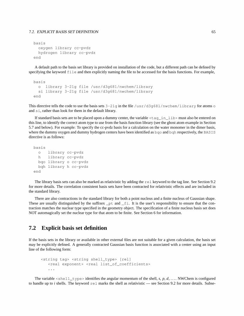
7.2. EXPLICIT BASIS SET DEFINITION 65
basisoxygen library cc-pvdzhydrogen library cc-pvdz
end
A default path to the basis set library is provided on installation of the code, but a different path can be defined byspecifying the keywordfile and then explicitly naming the file to be accessed for the basis functions. For example,
basiso library 3-21g file /usr/d3g681/nwchem/librarysi library 3-21g file /usr/d3g681/nwchem/library
end
This directive tells the code to use the basis sets3-21g in the file/usr/d3g681/nwchem/library for atomsoandsi , rather than look for them in the default library.
If standard basis sets are to be placed upon a dummy center, the variable<tag_in_lib> must also be entered onthis line, to identify the correct atom type to use from the basis function library (see the ghost atom example in Section5.7 and below). For example: To specify the cc-pvdz basis for a calculation on the water monomer in the dimer basis,where the dummy oxygen and dummy hydrogen centers have been identified asbqo andbqh respectively, theBASISdirective is as follows:
basiso library cc-pvdzh library cc-pvdzbqo library o cc-pvdzbqh library h cc-pvdz
end
The library basis sets can also be marked as relativistic by adding therel keyword to the tag line. See Section 9.2for more details. The correlation consistent basis sets have been contracted for relativistic effects and are included inthe standard library.
There are also contractions in the standard library for both a point nucleus and a finite nucleus of Gaussian shape.These are usually distinguished by the suffixex_pt and_fi . It is the user’s responsibility to ensure that the con-traction matches the nuclear type specified in the geometry object. The specification of a finite nucleus basis set doesNOT automagically set the nuclear type for that atom to be finite. See Section 6 for information.
7.2 Explicit basis set definition
If the basis sets in the library or available in other external files are not suitable for a given calculation, the basis setmay be explicitly defined. A generally contracted Gaussian basis function is associated with a center using an inputline of the following form:
<string tag> <string shell_type> [rel]<real exponent> <real list_of_coefficients>...
The variable<shell_type> identifies the angular momentum of the shell,s, p, d, . . . . NWChem is configuredto handle up toi shells. The keywordrel marks the shell as relativistic — see Section 9.2 for more details. Subse-
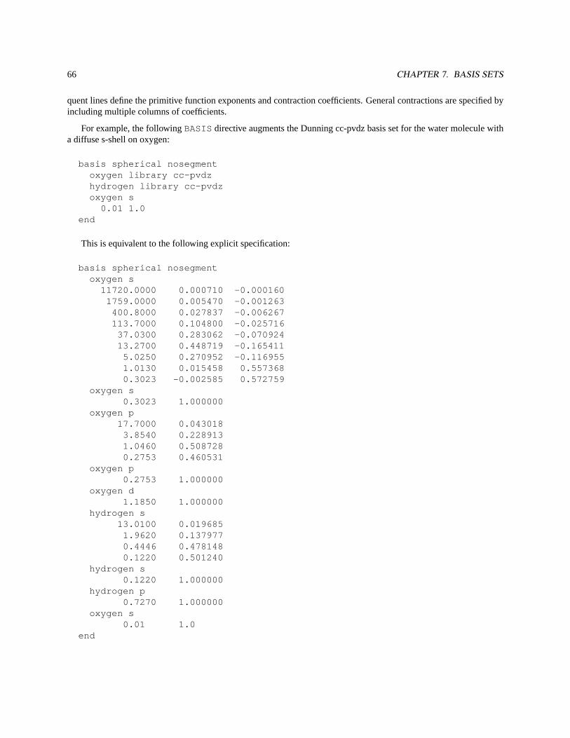
66 CHAPTER 7. BASIS SETS
quent lines define the primitive function exponents and contraction coefficients. General contractions are specified byincluding multiple columns of coefficients.
For example, the followingBASIS directive augments the Dunning cc-pvdz basis set for the water molecule witha diffuse s-shell on oxygen:
basis spherical nosegmentoxygen library cc-pvdzhydrogen library cc-pvdzoxygen s
0.01 1.0end
This is equivalent to the following explicit specification:
basis spherical nosegmentoxygen s
11720.0000 0.000710 -0.0001601759.0000 0.005470 -0.001263
400.8000 0.027837 -0.006267113.7000 0.104800 -0.025716
37.0300 0.283062 -0.07092413.2700 0.448719 -0.165411
5.0250 0.270952 -0.1169551.0130 0.015458 0.5573680.3023 -0.002585 0.572759
oxygen s0.3023 1.000000
oxygen p17.7000 0.043018
3.8540 0.2289131.0460 0.5087280.2753 0.460531
oxygen p0.2753 1.000000
oxygen d1.1850 1.000000
hydrogen s13.0100 0.019685
1.9620 0.1379770.4446 0.4781480.1220 0.501240
hydrogen s0.1220 1.000000
hydrogen p0.7270 1.000000
oxygen s0.01 1.0
end
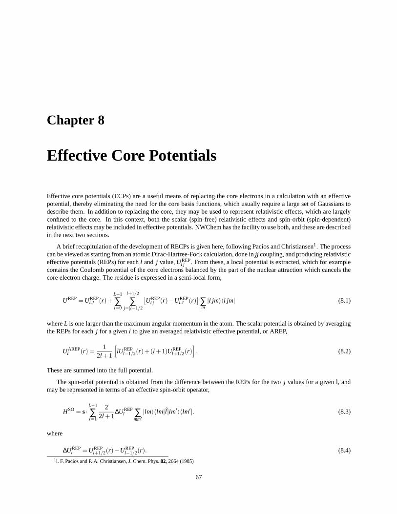
Chapter 8
Effective Core Potentials
Effective core potentials (ECPs) are a useful means of replacing the core electrons in a calculation with an effectivepotential, thereby eliminating the need for the core basis functions, which usually require a large set of Gaussians todescribe them. In addition to replacing the core, they may be used to represent relativistic effects, which are largelyconfined to the core. In this context, both the scalar (spin-free) relativistic effects and spin-orbit (spin-dependent)relativistic effects may be included in effective potentials. NWChem has the facility to use both, and these are describedin the next two sections.
A brief recapitulation of the development of RECPs is given here, following Pacios and Christiansen1. The processcan be viewed as starting from an atomic Dirac-Hartree-Fock calculation, done injj coupling, and producing relativisticeffective potentials (REPs) for eachl and j value,UREP
l j . From these, a local potential is extracted, which for examplecontains the Coulomb potential of the core electrons balanced by the part of the nuclear attraction which cancels thecore electron charge. The residue is expressed in a semi-local form,
UREP= UREPLJ (r)+
L−1
∑l=0
l+1/2
∑j=|l−1/2
[UREP
l j (r)−UREPLJ (r)
]∑m|l jm〉〈l jm| (8.1)
whereL is one larger than the maximum angular momentum in the atom. The scalar potential is obtained by averagingthe REPs for eachj for a givenl to give an averaged relativistic effective potential, or AREP,
UAREPl (r) =
12l +1
[lU REP
l−1/2(r)+(l +1)UREPl+1/2(r)
]. (8.2)
These are summed into the full potential.
The spin-orbit potential is obtained from the difference between the REPs for the twoj values for a given l, andmay be represented in terms of an effective spin-orbit operator,
HSO = s·L−1
∑l=1
22l +1
∆UREPl ∑
mm′|lm〉〈lm|l |lm′〉〈lm′|. (8.3)
where
∆UREPl = UREP
l+1/2(r)−UREPl−1/2(r). (8.4)
1l. F. Pacios and P. A. Christiansen, J. Chem. Phys.82, 2664 (1985)
67
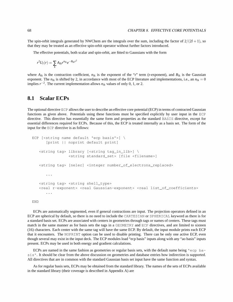
68 CHAPTER 8. EFFECTIVE CORE POTENTIALS
The spin-orbit integrals generated by NWChem are the integrals over the sum, including the factor of 2/(2l + 1), sothat they may be treated as an effective spin-orbit operator without further factors introduced.
The effective potentials, both scalar and spin-orbit, are fitted to Gaussians with the form
r2Ul (r) = ∑k
Alkrnlke−Blkr2
whereAlk is the contraction coefficient,nlk is the exponent of the “r” term (r-exponent), andBlk is the Gaussianexponent. Thenlk is shifted by 2, in accordance with most of the ECP literature and implementations, i.e., annlk = 0impliesr−2. The current implementation allowsnlk values of only 0, 1, or 2.
8.1 Scalar ECPs
The optional directiveECPallows the user to describe an effective core potential (ECP) in terms of contracted Gaussianfunctions as given above. Potentials using these functions must be specified explicitly by user input in theECPdirective. This directive has essentially the same form and properties as the standardBASIS directive, except foressential differences required for ECPs. Because of this, the ECP is treated internally as a basis set. The form of theinput for theECPdirective is as follows:
ECP [<string name default "ecp basis">] \[print || noprint default print]
<string tag> library [<string tag_in_lib>] \<string standard_set> [file <filename>]
<string tag> [nelec] <integer number_of_electrons_replaced>
...
<string tag> <string shell_type><real r-exponent> <real Gaussian-exponent> <real list_of_coefficients>
...
END
ECPs are automatically segmented, even if general contractions are input. The projection operators defined in anECP are spherical by default, so there is no need to include theCARTESIANor SPHERICALkeyword as there is fora standard basis set. ECPs are associated with centers in geometries through tags or names of centers. These tags mustmatch in the same manner as for basis sets the tags in aGEOMETRYandECPdirectives, and are limited to sixteen(16) characters. Each center with the same tag will have the same ECP. By default, the input module prints each ECPthat it encounters. TheNOPRINToption can be used to disable printing. There can be only one active ECP, eventhough several may exist in the input deck. The ECP modules load “ecp basis” inputs along with any “ao basis” inputspresent. ECPs may be used in both energy and gradient calculations.
ECPs are named in the same fashion as geometries or regular basis sets, with the default name being"ecp ba-sis" . It should be clear from the above discussion on geometries and database entries how indirection is supported.All directives that are in common with the standard Gaussian basis set input have the same function and syntax.
As for regular basis sets, ECPs may be obtained from the standard library. The names of the sets of ECPs availablein the standard library (their coverage is described in Appendix A) are
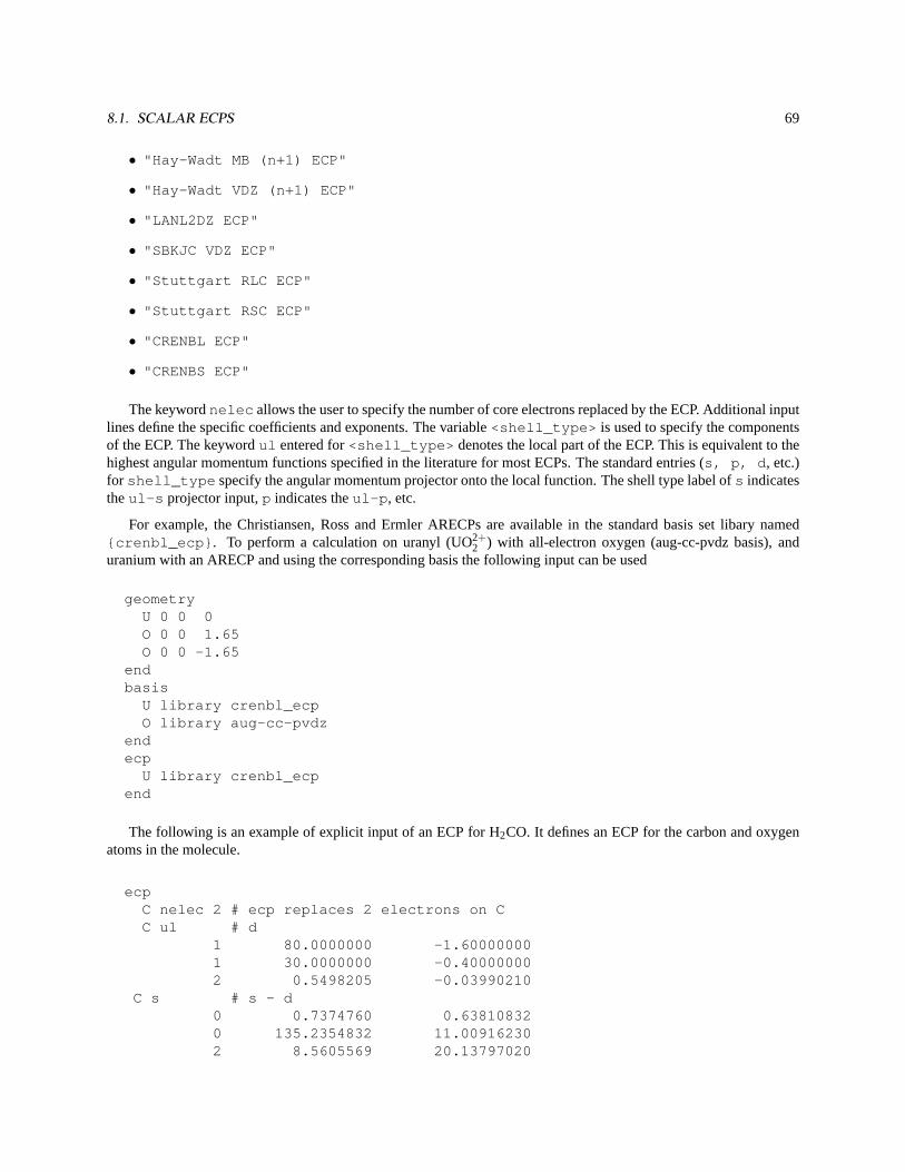
8.1. SCALAR ECPS 69
• "Hay-Wadt MB (n+1) ECP"
• "Hay-Wadt VDZ (n+1) ECP"
• "LANL2DZ ECP"
• "SBKJC VDZ ECP"
• "Stuttgart RLC ECP"
• "Stuttgart RSC ECP"
• "CRENBL ECP"
• "CRENBS ECP"
The keywordnelec allows the user to specify the number of core electrons replaced by the ECP. Additional inputlines define the specific coefficients and exponents. The variable<shell_type> is used to specify the componentsof the ECP. The keywordul entered for<shell_type> denotes the local part of the ECP. This is equivalent to thehighest angular momentum functions specified in the literature for most ECPs. The standard entries (s, p, d , etc.)for shell_type specify the angular momentum projector onto the local function. The shell type label ofs indicatestheul-s projector input,p indicates theul-p , etc.
For example, the Christiansen, Ross and Ermler ARECPs are available in the standard basis set libary named{crenbl_ecp} . To perform a calculation on uranyl (UO2+
2 ) with all-electron oxygen (aug-cc-pvdz basis), anduranium with an ARECP and using the corresponding basis the following input can be used
geometryU 0 0 0O 0 0 1.65O 0 0 -1.65
endbasis
U library crenbl_ecpO library aug-cc-pvdz
endecp
U library crenbl_ecpend
The following is an example of explicit input of an ECP for H2CO. It defines an ECP for the carbon and oxygenatoms in the molecule.
ecpC nelec 2 # ecp replaces 2 electrons on CC ul # d
1 80.0000000 -1.600000001 30.0000000 -0.400000002 0.5498205 -0.03990210
C s # s - d0 0.7374760 0.638108320 135.2354832 11.009162302 8.5605569 20.13797020
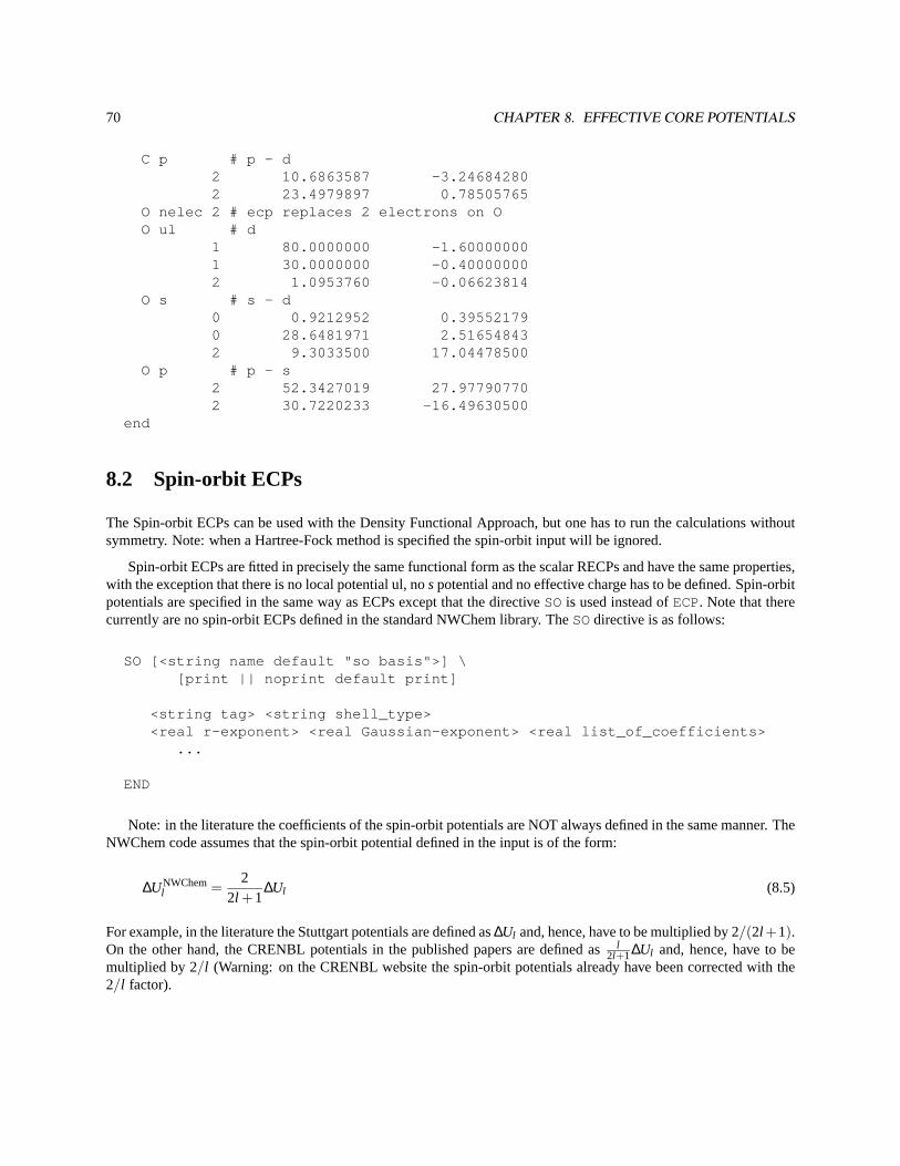
70 CHAPTER 8. EFFECTIVE CORE POTENTIALS
C p # p - d2 10.6863587 -3.246842802 23.4979897 0.78505765
O nelec 2 # ecp replaces 2 electrons on OO ul # d
1 80.0000000 -1.600000001 30.0000000 -0.400000002 1.0953760 -0.06623814
O s # s - d0 0.9212952 0.395521790 28.6481971 2.516548432 9.3033500 17.04478500
O p # p - s2 52.3427019 27.977907702 30.7220233 -16.49630500
end
8.2 Spin-orbit ECPs
The Spin-orbit ECPs can be used with the Density Functional Approach, but one has to run the calculations withoutsymmetry. Note: when a Hartree-Fock method is specified the spin-orbit input will be ignored.
Spin-orbit ECPs are fitted in precisely the same functional form as the scalar RECPs and have the same properties,with the exception that there is no local potential ul, nospotential and no effective charge has to be defined. Spin-orbitpotentials are specified in the same way as ECPs except that the directiveSOis used instead ofECP. Note that therecurrently are no spin-orbit ECPs defined in the standard NWChem library. TheSOdirective is as follows:
SO [<string name default "so basis">] \[print || noprint default print]
<string tag> <string shell_type><real r-exponent> <real Gaussian-exponent> <real list_of_coefficients>
...
END
Note: in the literature the coefficients of the spin-orbit potentials are NOT always defined in the same manner. TheNWChem code assumes that the spin-orbit potential defined in the input is of the form:
∆UNWCheml =
22l +1
∆Ul (8.5)
For example, in the literature the Stuttgart potentials are defined as∆Ul and, hence, have to be multiplied by 2/(2l +1).On the other hand, the CRENBL potentials in the published papers are defined asl
2l+1∆Ul and, hence, have to bemultiplied by 2/l (Warning: on the CRENBL website the spin-orbit potentials already have been corrected with the2/l factor).
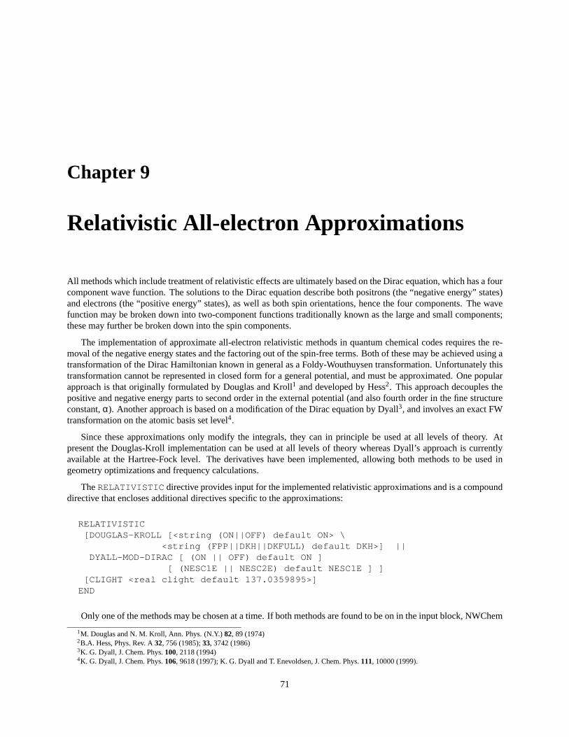
Chapter 9
Relativistic All-electron Approximations
All methods which include treatment of relativistic effects are ultimately based on the Dirac equation, which has a fourcomponent wave function. The solutions to the Dirac equation describe both positrons (the “negative energy” states)and electrons (the “positive energy” states), as well as both spin orientations, hence the four components. The wavefunction may be broken down into two-component functions traditionally known as the large and small components;these may further be broken down into the spin components.
The implementation of approximate all-electron relativistic methods in quantum chemical codes requires the re-moval of the negative energy states and the factoring out of the spin-free terms. Both of these may be achieved using atransformation of the Dirac Hamiltonian known in general as a Foldy-Wouthuysen transformation. Unfortunately thistransformation cannot be represented in closed form for a general potential, and must be approximated. One popularapproach is that originally formulated by Douglas and Kroll1 and developed by Hess2. This approach decouples thepositive and negative energy parts to second order in the external potential (and also fourth order in the fine structureconstant,α). Another approach is based on a modification of the Dirac equation by Dyall3, and involves an exact FWtransformation on the atomic basis set level4.
Since these approximations only modify the integrals, they can in principle be used at all levels of theory. Atpresent the Douglas-Kroll implementation can be used at all levels of theory whereas Dyall’s approach is currentlyavailable at the Hartree-Fock level. The derivatives have been implemented, allowing both methods to be used ingeometry optimizations and frequency calculations.
TheRELATIVISTIC directive provides input for the implemented relativistic approximations and is a compounddirective that encloses additional directives specific to the approximations:
RELATIVISTIC[DOUGLAS-KROLL [<string (ON||OFF) default ON> \
<string (FPP||DKH||DKFULL) default DKH>] ||DYALL-MOD-DIRAC [ (ON || OFF) default ON ]
[ (NESC1E || NESC2E) default NESC1E ] ][CLIGHT <real clight default 137.0359895>]
END
Only one of the methods may be chosen at a time. If both methods are found to be on in the input block, NWChem
1M. Douglas and N. M. Kroll, Ann. Phys. (N.Y.)82, 89 (1974)2B.A. Hess, Phys. Rev. A32, 756 (1985);33, 3742 (1986)3K. G. Dyall, J. Chem. Phys.100, 2118 (1994)4K. G. Dyall, J. Chem. Phys.106, 9618 (1997); K. G. Dyall and T. Enevoldsen, J. Chem. Phys.111, 10000 (1999).
71
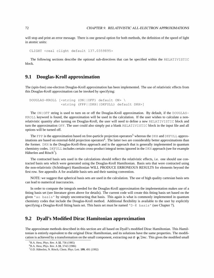
72 CHAPTER 9. RELATIVISTIC ALL-ELECTRON APPROXIMATIONS
will stop and print an error message. There is one general option for both methods, the definition of the speed of lightin atomic units:
CLIGHT <real clight default 137.0359895>
The following sections describe the optional sub-directives that can be specified within theRELATIVISTICblock.
9.1 Douglas-Kroll approximation
The (spin-free) one-electron Douglas-Kroll approximation has been implemented. The use of relativistic effects fromthis Douglas-Kroll approximation can be invoked by specifying:
DOUGLAS-KROLL [<string (ON||OFF) default ON> \<string (FPP||DKH||DKFULL) default DKH>]
The ON|OFF string is used to turn on or off the Douglas-Kroll approximation. By default, if theDOUGLAS-KROLLkeyword is found, the approximation will be used in the calculation. If the user wishes to calculate a non-relativistic quantity after turning on Douglas-Kroll, the user will need to define a newRELATIVISTIC block andturn the approximationOFF. The user could also simply put a blankRELATIVISTIC block in the input file and alloptions will be turned off.
TheFPP is the approximation based on free-particle projection operators5 whereas theDKHandDKFULLapprox-imations are based on external-field projection operators6. The latter two are considerably better approximations thanthe former.DKHis the Douglas-Kroll-Hess approach and is the approach that is generally implemented in quantumchemistry codes.DKFULLincludes certain cross-product integral terms ignored in theDKHapproach (see for exampleHäberlen and Rösch7).
The contracted basis sets used in the calculations should reflect the relativistic effects, i.e. one should use con-tracted basis sets which were generated using the Douglas-Kroll Hamiltonian. Basis sets that were contracted usingthe non-relativistic (Schödinger) Hamiltonian WILL PRODUCE ERRONEOUS RESULTS for elements beyond thefirst row. See appendix A for available basis sets and their naming convention.
NOTE: we suggest that spherical basis sets are used in the calculation. The use of high quality cartesian basis setscan lead to numerical inaccuracies.
In order to compute the integrals needed for the Douglas-Kroll approximation the implementation makes use of afitting basis set (see literature given above for details). The current code will create this fitting basis set based on thegiven "ao basis" by simply uncontracting that basis. This again is what is commonly implemented in quantumchemistry codes that include the Douglas-Kroll method. Additional flexibility is available to the user by explicitlyspecifying a Douglas-Kroll fitting basis set. This basis set must be named"D-K basis" (see Chapter 7).
9.2 Dyall’s Modified Dirac Hamitonian approximation
The approximate methods described in this section are all based on Dyall’s modified Dirac Hamiltonian. This Hamil-tonian is entirely equivalent to the original Dirac Hamiltonian, and its solutions have the same properties. The modifi-cation is achieved by a transformation on the small component, extracting outσ ·p/2mc. This gives the modified small
5B.A. Hess, Phys. Rev. A32, 756 (1985)6B.A. Hess, Phys. Rev. A33, 3742 (1986)7O.D. Häberlen, N. Rösch, Chem. Phys. Lett.199, 491 (1992)
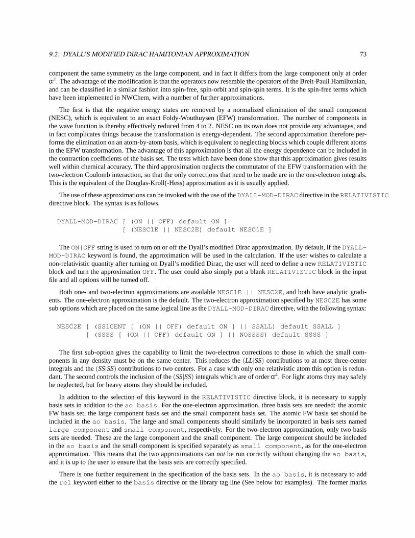
9.2. DYALL’S MODIFIED DIRAC HAMITONIAN APPROXIMATION 73
component the same symmetry as the large component, and in fact it differs from the large component only at orderα2. The advantage of the modification is that the operators now resemble the operators of the Breit-Pauli Hamiltonian,and can be classified in a similar fashion into spin-free, spin-orbit and spin-spin terms. It is the spin-free terms whichhave been implemented in NWChem, with a number of further approximations.
The first is that the negative energy states are removed by a normalized elimination of the small component(NESC), which is equivalent to an exact Foldy-Wouthuysen (EFW) transformation. The number of components inthe wave function is thereby effectively reduced from 4 to 2. NESC on its own does not provide any advantages, andin fact complicates things because the transformation is energy-dependent. The second approximation therefore per-forms the elimination on an atom-by-atom basis, which is equivalent to neglecting blocks which couple different atomsin the EFW transformation. The advantage of this approximation is that all the energy dependence can be included inthe contraction coefficients of the basis set. The tests which have been done show that this approximation gives resultswell within chemical accuracy. The third approximation neglects the commutator of the EFW transformation with thetwo-electron Coulomb interaction, so that the only corrections that need to be made are in the one-electron integrals.This is the equivalent of the Douglas-Kroll(-Hess) approximation as it is usually applied.
The use of these approximations can be invoked with the use of theDYALL-MOD-DIRACdirective in theRELATIVISTICdirective block. The syntax is as follows.
DYALL-MOD-DIRAC [ (ON || OFF) default ON ][ (NESC1E || NESC2E) default NESC1E ]
TheON|OFFstring is used to turn on or off the Dyall’s modified Dirac approximation. By default, if theDYALL-MOD-DIRACkeyword is found, the approximation will be used in the calculation. If the user wishes to calculate anon-relativistic quantity after turning on Dyall’s modified Dirac, the user will need to define a newRELATIVISTICblock and turn the approximationOFF. The user could also simply put a blankRELATIVISTIC block in the inputfile and all options will be turned off.
Both one- and two-electron approximations are availableNESC1E || NESC2E, and both have analytic gradi-ents. The one-electron approximation is the default. The two-electron approximation specified byNESC2Ehas somesub options which are placed on the same logical line as theDYALL-MOD-DIRACdirective, with the following syntax:
NESC2E [ (SS1CENT [ (ON || OFF) default ON ] || SSALL) default SSALL ][ (SSSS [ (ON || OFF) default ON ] || NOSSSS) default SSSS ]
The first sub-option gives the capability to limit the two-electron corrections to those in which the small com-ponents in any density must be on the same center. This reduces the(LL|SS) contributions to at most three-centerintegrals and the(SS|SS) contributions to two centers. For a case with only one relativistic atom this option is redun-dant. The second controls the inclusion of the(SS|SS) integrals which are of orderα4. For light atoms they may safelybe neglected, but for heavy atoms they should be included.
In addition to the selection of this keyword in theRELATIVISTIC directive block, it is necessary to supplybasis sets in addition to theao basis . For the one-electron approximation, three basis sets are needed: the atomicFW basis set, the large component basis set and the small component basis set. The atomic FW basis set should beincluded in theao basis . The large and small components should similarly be incorporated in basis sets namedlarge component andsmall component , respectively. For the two-electron approximation, only two basissets are needed. These are the large component and the small component. The large component should be includedin theao basis and the small component is specified separately assmall component , as for the one-electronapproximation. This means that the two approximations cannot be run correctly without changing theao basis ,and it is up to the user to ensure that the basis sets are correctly specified.
There is one further requirement in the specification of the basis sets. In theao basis , it is necessary to addthe rel keyword either to thebasis directive or the library tag line (See below for examples). The former marks
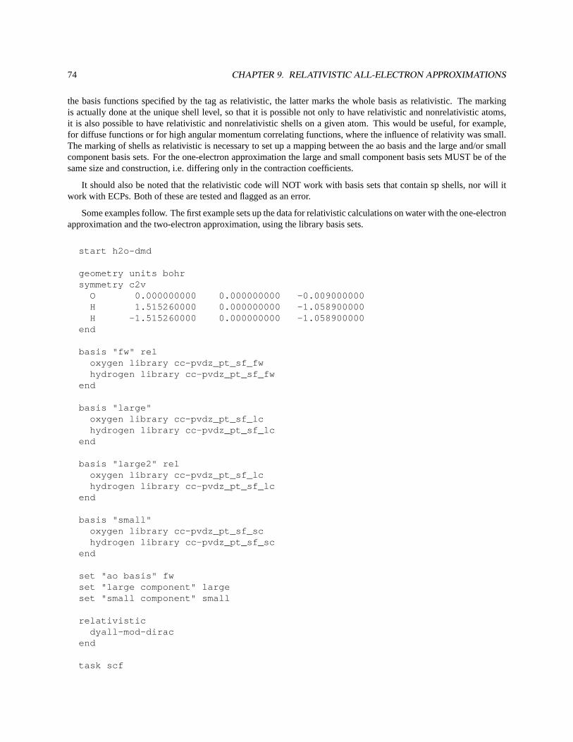
74 CHAPTER 9. RELATIVISTIC ALL-ELECTRON APPROXIMATIONS
the basis functions specified by the tag as relativistic, the latter marks the whole basis as relativistic. The markingis actually done at the unique shell level, so that it is possible not only to have relativistic and nonrelativistic atoms,it is also possible to have relativistic and nonrelativistic shells on a given atom. This would be useful, for example,for diffuse functions or for high angular momentum correlating functions, where the influence of relativity was small.The marking of shells as relativistic is necessary to set up a mapping between the ao basis and the large and/or smallcomponent basis sets. For the one-electron approximation the large and small component basis sets MUST be of thesame size and construction, i.e. differing only in the contraction coefficients.
It should also be noted that the relativistic code will NOT work with basis sets that contain sp shells, nor will itwork with ECPs. Both of these are tested and flagged as an error.
Some examples follow. The first example sets up the data for relativistic calculations on water with the one-electronapproximation and the two-electron approximation, using the library basis sets.
start h2o-dmd
geometry units bohrsymmetry c2v
O 0.000000000 0.000000000 -0.009000000H 1.515260000 0.000000000 -1.058900000H -1.515260000 0.000000000 -1.058900000
end
basis "fw" reloxygen library cc-pvdz_pt_sf_fwhydrogen library cc-pvdz_pt_sf_fw
end
basis "large"oxygen library cc-pvdz_pt_sf_lchydrogen library cc-pvdz_pt_sf_lc
end
basis "large2" reloxygen library cc-pvdz_pt_sf_lchydrogen library cc-pvdz_pt_sf_lc
end
basis "small"oxygen library cc-pvdz_pt_sf_schydrogen library cc-pvdz_pt_sf_sc
end
set "ao basis" fwset "large component" largeset "small component" small
relativisticdyall-mod-dirac
end
task scf
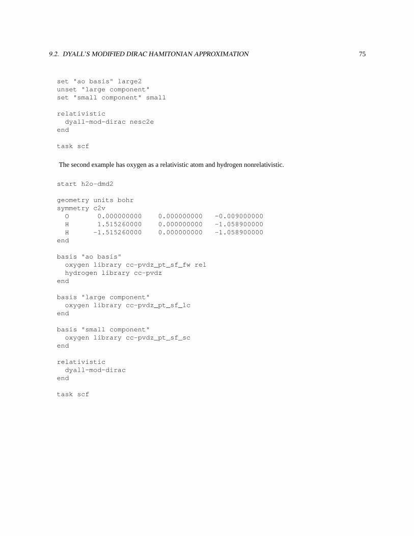
9.2. DYALL’S MODIFIED DIRAC HAMITONIAN APPROXIMATION 75
set "ao basis" large2unset "large component"set "small component" small
relativisticdyall-mod-dirac nesc2e
end
task scf
The second example has oxygen as a relativistic atom and hydrogen nonrelativistic.
start h2o-dmd2
geometry units bohrsymmetry c2v
O 0.000000000 0.000000000 -0.009000000H 1.515260000 0.000000000 -1.058900000H -1.515260000 0.000000000 -1.058900000
end
basis "ao basis"oxygen library cc-pvdz_pt_sf_fw relhydrogen library cc-pvdz
end
basis "large component"oxygen library cc-pvdz_pt_sf_lc
end
basis "small component"oxygen library cc-pvdz_pt_sf_sc
end
relativisticdyall-mod-dirac
end
task scf

76 CHAPTER 9. RELATIVISTIC ALL-ELECTRON APPROXIMATIONS
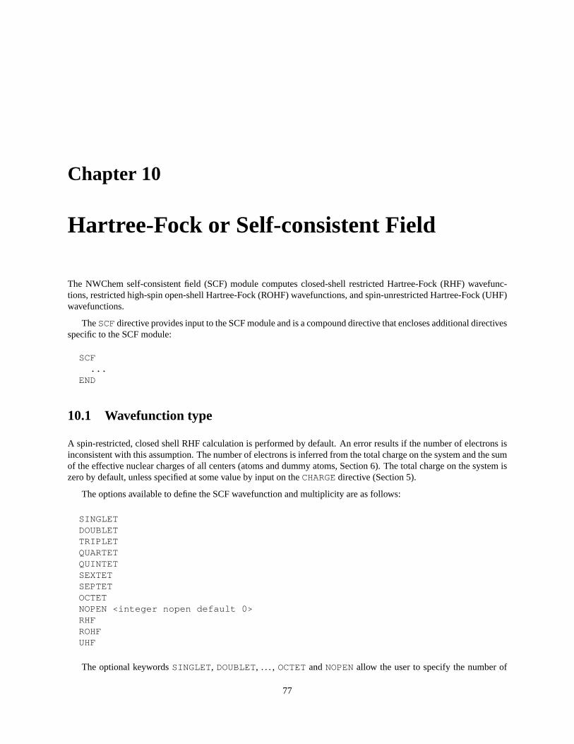
Chapter 10
Hartree-Fock or Self-consistent Field
The NWChem self-consistent field (SCF) module computes closed-shell restricted Hartree-Fock (RHF) wavefunc-tions, restricted high-spin open-shell Hartree-Fock (ROHF) wavefunctions, and spin-unrestricted Hartree-Fock (UHF)wavefunctions.
TheSCFdirective provides input to the SCF module and is a compound directive that encloses additional directivesspecific to the SCF module:
SCF...
END
10.1 Wavefunction type
A spin-restricted, closed shell RHF calculation is performed by default. An error results if the number of electrons isinconsistent with this assumption. The number of electrons is inferred from the total charge on the system and the sumof the effective nuclear charges of all centers (atoms and dummy atoms, Section 6). The total charge on the system iszero by default, unless specified at some value by input on theCHARGEdirective (Section 5).
The options available to define the SCF wavefunction and multiplicity are as follows:
SINGLETDOUBLETTRIPLETQUARTETQUINTETSEXTETSEPTETOCTETNOPEN <integer nopen default 0>RHFROHFUHF
The optional keywordsSINGLET, DOUBLET, . . . , OCTETandNOPENallow the user to specify the number of
77
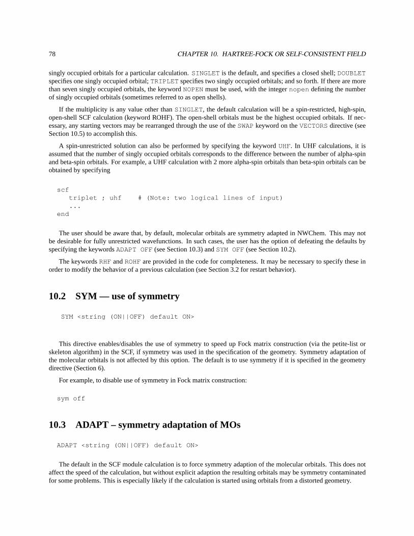
78 CHAPTER 10. HARTREE-FOCK OR SELF-CONSISTENT FIELD
singly occupied orbitals for a particular calculation.SINGLET is the default, and specifies a closed shell;DOUBLETspecifies one singly occupied orbital;TRIPLET specifies two singly occupied orbitals; and so forth. If there are morethan seven singly occupied orbitals, the keywordNOPENmust be used, with the integernopen defining the numberof singly occupied orbitals (sometimes referred to as open shells).
If the multiplicity is any value other thanSINGLET, the default calculation will be a spin-restricted, high-spin,open-shell SCF calculation (keyword ROHF). The open-shell orbitals must be the highest occupied orbitals. If nec-essary, any starting vectors may be rearranged through the use of theSWAPkeyword on theVECTORSdirective (seeSection 10.5) to accomplish this.
A spin-unrestricted solution can also be performed by specifying the keywordUHF. In UHF calculations, it isassumed that the number of singly occupied orbitals corresponds to the difference between the number of alpha-spinand beta-spin orbitals. For example, a UHF calculation with 2 more alpha-spin orbitals than beta-spin orbitals can beobtained by specifying
scftriplet ; uhf # (Note: two logical lines of input)...
end
The user should be aware that, by default, molecular orbitals are symmetry adapted in NWChem. This may notbe desirable for fully unrestricted wavefunctions. In such cases, the user has the option of defeating the defaults byspecifying the keywordsADAPT OFF(see Section 10.3) andSYM OFF(see Section 10.2).
The keywordsRHFandROHFare provided in the code for completeness. It may be necessary to specify these inorder to modify the behavior of a previous calculation (see Section 3.2 for restart behavior).
10.2 SYM — use of symmetry
SYM <string (ON||OFF) default ON>
This directive enables/disables the use of symmetry to speed up Fock matrix construction (via the petite-list orskeleton algorithm) in the SCF, if symmetry was used in the specification of the geometry. Symmetry adaptation ofthe molecular orbitals is not affected by this option. The default is to use symmetry if it is specified in the geometrydirective (Section 6).
For example, to disable use of symmetry in Fock matrix construction:
sym off
10.3 ADAPT – symmetry adaptation of MOs
ADAPT <string (ON||OFF) default ON>
The default in the SCF module calculation is to force symmetry adaption of the molecular orbitals. This does notaffect the speed of the calculation, but without explicit adaption the resulting orbitals may be symmetry contaminatedfor some problems. This is especially likely if the calculation is started using orbitals from a distorted geometry.
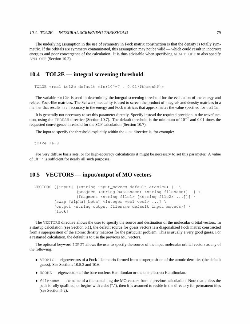
10.4. TOL2E — INTEGRAL SCREENING THRESHOLD 79
The underlying assumption in the use of symmetry in Fock matrix construction is that the density is totally sym-metric. If the orbitals are symmetry contaminated, this assumption may not be valid — which could result in incorrectenergies and poor convergence of the calculation. It is thus advisable when specifyingADAPT OFFto also specifySYM OFF(Section 10.2).
10.4 TOL2E — integral screening threshold
TOL2E <real tol2e default min(10^-7 , 0.01*$thresh$)>
The variabletol2e is used in determining the integral screening threshold for the evaluation of the energy andrelated Fock-like matrices. The Schwarz inequality is used to screen the product of integrals and density matrices in amanner that results in an accuracy in the energy and Fock matrices that approximates the value specified fortol2e .
It is generally not necessary to set this parameter directly. Specify instead the required precision in the wavefunc-tion, using theTHRESHdirective (Section 10.7). The default threshold is the minimum of 10−7 and 0.01 times therequested convergence threshold for the SCF calculation (Section 10.7).
The input to specify the threshold explicitly within theSCFdirective is, for example:
tol2e 1e-9
For very diffuse basis sets, or for high-accuracy calculations it might be necessary to set this parameter. A valueof 10−12 is sufficient for nearly all such purposes.
10.5 VECTORS — input/output of MO vectors
VECTORS [[input] (<string input_movecs default atomic>) || \(project <string basisname> <string filename>) || \(fragment <string file1> [<string file2> ...])] \
[swap [alpha||beta] <integer vec1 vec2> ...] \[output <string output_filename default input_movecs>] \[lock]
TheVECTORSdirective allows the user to specify the source and destination of the molecular orbital vectors. Ina startup calculation (see Section 5.1), the default source for guess vectors is a diagonalized Fock matrix constructedfrom a superposition of the atomic density matrices for the particular problem. This is usually a very good guess. Fora restarted calculation, the default is to use the previous MO vectors.
The optional keywordINPUT allows the user to specify the source of the input molecular orbital vectors as any ofthe following:
• ATOMIC— eigenvectors of a Fock-like matrix formed from a superposition of the atomic densities (the defaultguess). See Sections 10.5.2 and 10.6.
• HCORE— eigenvectors of the bare-nucleus Hamiltonian or the one-electron Hamiltonian.
• filename — the name of a file containing the MO vectors from a previous calculation. Note that unless thepath is fully qualified, or begins with a dot (“.”), then it is assumed to reside in the directory for permanent files(see Section 5.2).
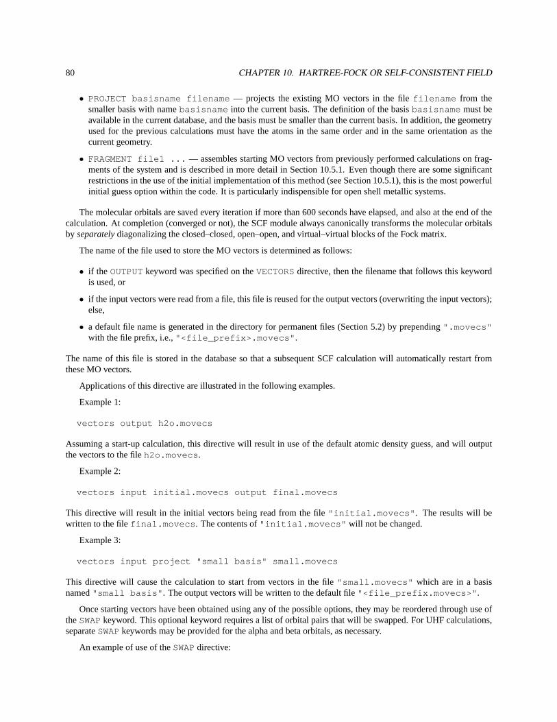
80 CHAPTER 10. HARTREE-FOCK OR SELF-CONSISTENT FIELD
• PROJECT basisname filename — projects the existing MO vectors in the filefilename from thesmaller basis with namebasisname into the current basis. The definition of the basisbasisname must beavailable in the current database, and the basis must be smaller than the current basis. In addition, the geometryused for the previous calculations must have the atoms in the same order and in the same orientation as thecurrent geometry.
• FRAGMENT file1 ... — assembles starting MO vectors from previously performed calculations on frag-ments of the system and is described in more detail in Section 10.5.1. Even though there are some significantrestrictions in the use of the initial implementation of this method (see Section 10.5.1), this is the most powerfulinitial guess option within the code. It is particularly indispensible for open shell metallic systems.
The molecular orbitals are saved every iteration if more than 600 seconds have elapsed, and also at the end of thecalculation. At completion (converged or not), the SCF module always canonically transforms the molecular orbitalsby separatelydiagonalizing the closed–closed, open–open, and virtual–virtual blocks of the Fock matrix.
The name of the file used to store the MO vectors is determined as follows:
• if the OUTPUTkeyword was specified on theVECTORSdirective, then the filename that follows this keywordis used, or
• if the input vectors were read from a file, this file is reused for the output vectors (overwriting the input vectors);else,
• a default file name is generated in the directory for permanent files (Section 5.2) by prepending".movecs"with the file prefix, i.e.,"<file_prefix>.movecs" .
The name of this file is stored in the database so that a subsequent SCF calculation will automatically restart fromthese MO vectors.
Applications of this directive are illustrated in the following examples.
Example 1:
vectors output h2o.movecs
Assuming a start-up calculation, this directive will result in use of the default atomic density guess, and will outputthe vectors to the fileh2o.movecs .
Example 2:
vectors input initial.movecs output final.movecs
This directive will result in the initial vectors being read from the file"initial.movecs" . The results will bewritten to the filefinal.movecs . The contents of"initial.movecs" will not be changed.
Example 3:
vectors input project "small basis" small.movecs
This directive will cause the calculation to start from vectors in the file"small.movecs" which are in a basisnamed"small basis" . The output vectors will be written to the default file"<file_prefix.movecs>" .
Once starting vectors have been obtained using any of the possible options, they may be reordered through use oftheSWAPkeyword. This optional keyword requires a list of orbital pairs that will be swapped. For UHF calculations,separateSWAPkeywords may be provided for the alpha and beta orbitals, as necessary.
An example of use of theSWAPdirective:
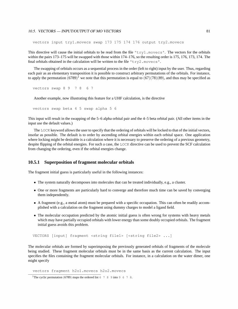
10.5. VECTORS — INPUT/OUTPUT OF MO VECTORS 81
vectors input try1.movecs swap 173 175 174 176 output try2.movecs
This directive will cause the initial orbitals to be read from the file"try1.movecs" . The vectors for the orbitalswithin the pairs 173–175 will be swapped with those within 174–176, so the resulting order is 175, 176, 173, 174. Thefinal orbitals obtained in the calculation will be written to the file"try2.movecs" .
The swapping of orbitals occurs as a sequential process in the order (left to right) input by the user. Thus, regardingeach pair as an elementary transposition it is possible to construct arbitrary permutations of the orbitals. For instance,to apply the permutation(6789)1 we note that this permutation is equal to(67)(78)(89), and thus may be specified as
vectors swap 8 9 7 8 6 7
Another example, now illustrating this feature for a UHF calculation, is the directive
vectors swap beta 4 5 swap alpha 5 6
This input will result in the swapping of the 5–6 alpha orbital pair and the 4–5 beta orbital pair. (All other items in theinput use the default values.)
TheLOCKkeyword allows the user to specify that the ordering of orbitals will be locked to that of the initial vectors,insofar as possible. The default is to order by ascending orbital energies within each orbital space. One applicationwhere locking might be desirable is a calculation where it is necessary to preserve the ordering of a previous geometry,despite flipping of the orbital energies. For such a case, theLOCKdirective can be used to prevent the SCF calculationfrom changing the ordering, even if the orbital energies change.
10.5.1 Superposition of fragment molecular orbitals
The fragment initial guess is particularly useful in the following instances:
• The system naturally decomposes into molecules that can be treated individually, e.g., a cluster.
• One or more fragments are particularly hard to converge and therefore much time can be saved by convergingthem independently.
• A fragment (e.g., a metal atom) must be prepared with a specific occupation. This can often be readily accom-plished with a calculation on the fragment using dummy charges to model a ligand field.
• The molecular occupation predicted by the atomic initial guess is often wrong for systems with heavy metalswhich may have partially occupied orbitals with lower energy than some doubly occupied orbitals. The fragmentinitial guess avoids this problem.
VECTORS [input] fragment <string file1> [<string file2> ...]
The molecular orbitals are formed by superimposing the previously generated orbitals of fragments of the moleculebeing studied. These fragment molecular orbitals must be in the same basis as the current calculation. The inputspecifies the files containing the fragment molecular orbitals. For instance, in a calculation on the water dimer, onemight specify
vectors fragment h2o1.movecs h2o2.movecs
1The cyclic permutation(6789) maps the ordered list6 7 8 9 into 9 6 7 8 .
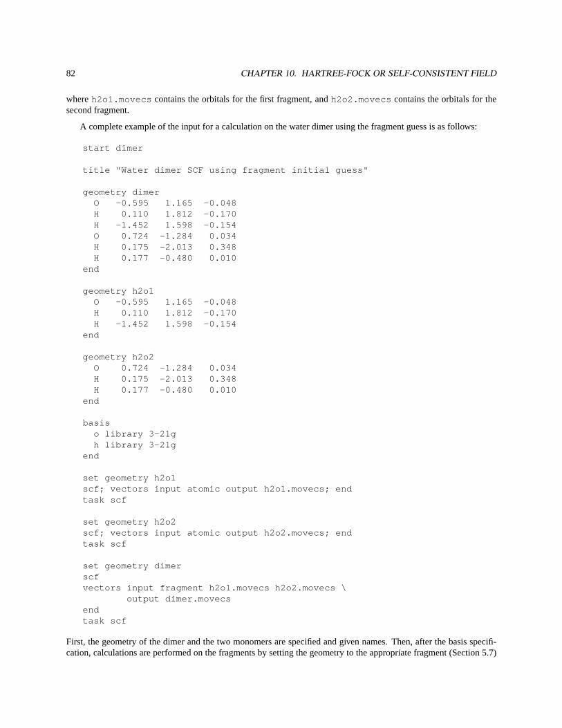
82 CHAPTER 10. HARTREE-FOCK OR SELF-CONSISTENT FIELD
whereh2o1.movecs contains the orbitals for the first fragment, andh2o2.movecs contains the orbitals for thesecond fragment.
A complete example of the input for a calculation on the water dimer using the fragment guess is as follows:
start dimer
title "Water dimer SCF using fragment initial guess"
geometry dimerO -0.595 1.165 -0.048H 0.110 1.812 -0.170H -1.452 1.598 -0.154O 0.724 -1.284 0.034H 0.175 -2.013 0.348H 0.177 -0.480 0.010
end
geometry h2o1O -0.595 1.165 -0.048H 0.110 1.812 -0.170H -1.452 1.598 -0.154
end
geometry h2o2O 0.724 -1.284 0.034H 0.175 -2.013 0.348H 0.177 -0.480 0.010
end
basiso library 3-21gh library 3-21g
end
set geometry h2o1scf; vectors input atomic output h2o1.movecs; endtask scf
set geometry h2o2scf; vectors input atomic output h2o2.movecs; endtask scf
set geometry dimerscfvectors input fragment h2o1.movecs h2o2.movecs \
output dimer.movecsendtask scf
First, the geometry of the dimer and the two monomers are specified and given names. Then, after the basis specifi-cation, calculations are performed on the fragments by setting the geometry to the appropriate fragment (Section 5.7)
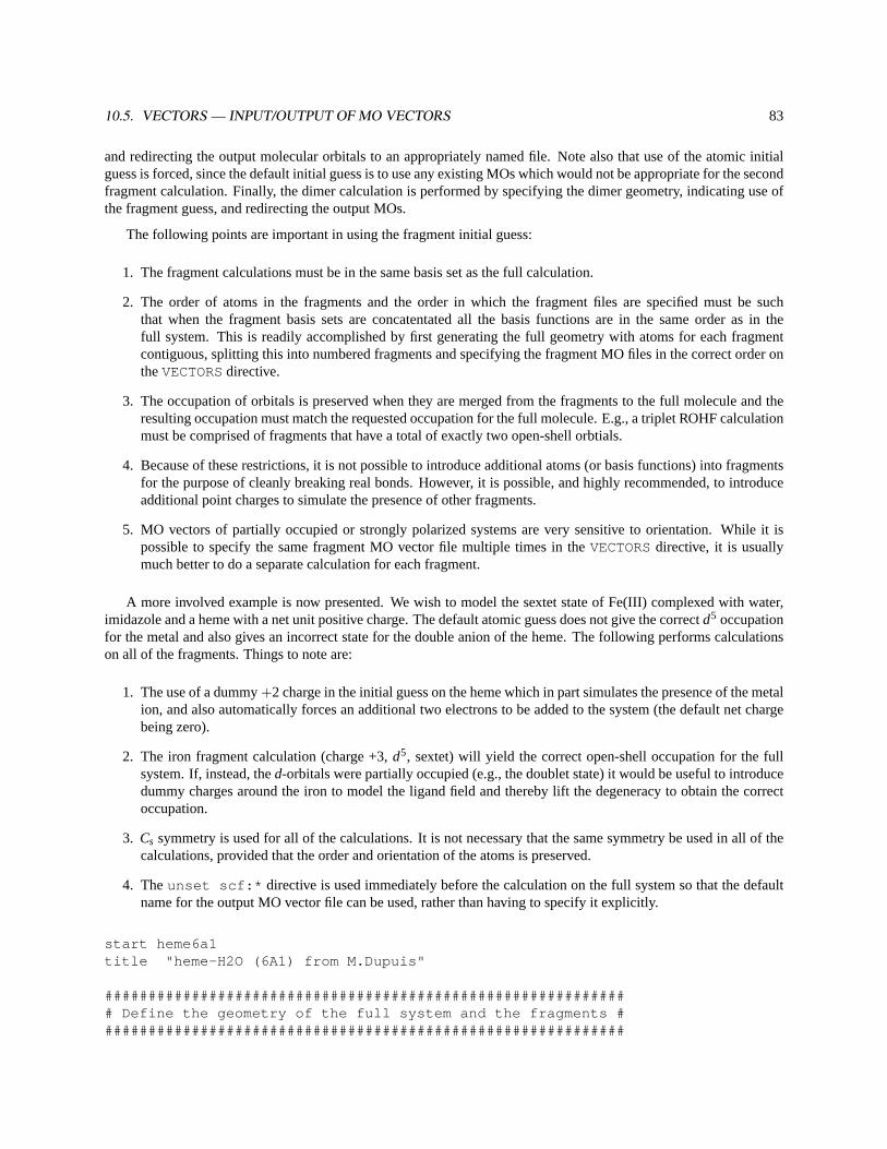
10.5. VECTORS — INPUT/OUTPUT OF MO VECTORS 83
and redirecting the output molecular orbitals to an appropriately named file. Note also that use of the atomic initialguess is forced, since the default initial guess is to use any existing MOs which would not be appropriate for the secondfragment calculation. Finally, the dimer calculation is performed by specifying the dimer geometry, indicating use ofthe fragment guess, and redirecting the output MOs.
The following points are important in using the fragment initial guess:
1. The fragment calculations must be in the same basis set as the full calculation.
2. The order of atoms in the fragments and the order in which the fragment files are specified must be suchthat when the fragment basis sets are concatentated all the basis functions are in the same order as in thefull system. This is readily accomplished by first generating the full geometry with atoms for each fragmentcontiguous, splitting this into numbered fragments and specifying the fragment MO files in the correct order ontheVECTORSdirective.
3. The occupation of orbitals is preserved when they are merged from the fragments to the full molecule and theresulting occupation must match the requested occupation for the full molecule. E.g., a triplet ROHF calculationmust be comprised of fragments that have a total of exactly two open-shell orbtials.
4. Because of these restrictions, it is not possible to introduce additional atoms (or basis functions) into fragmentsfor the purpose of cleanly breaking real bonds. However, it is possible, and highly recommended, to introduceadditional point charges to simulate the presence of other fragments.
5. MO vectors of partially occupied or strongly polarized systems are very sensitive to orientation. While it ispossible to specify the same fragment MO vector file multiple times in theVECTORSdirective, it is usuallymuch better to do a separate calculation for each fragment.
A more involved example is now presented. We wish to model the sextet state of Fe(III) complexed with water,imidazole and a heme with a net unit positive charge. The default atomic guess does not give the correctd5 occupationfor the metal and also gives an incorrect state for the double anion of the heme. The following performs calculationson all of the fragments. Things to note are:
1. The use of a dummy+2 charge in the initial guess on the heme which in part simulates the presence of the metalion, and also automatically forces an additional two electrons to be added to the system (the default net chargebeing zero).
2. The iron fragment calculation (charge +3,d5, sextet) will yield the correct open-shell occupation for the fullsystem. If, instead, thed-orbitals were partially occupied (e.g., the doublet state) it would be useful to introducedummy charges around the iron to model the ligand field and thereby lift the degeneracy to obtain the correctoccupation.
3. Cs symmetry is used for all of the calculations. It is not necessary that the same symmetry be used in all of thecalculations, provided that the order and orientation of the atoms is preserved.
4. Theunset scf:* directive is used immediately before the calculation on the full system so that the defaultname for the output MO vector file can be used, rather than having to specify it explicitly.
start heme6a1title "heme-H2O (6A1) from M.Dupuis"
############################################################# Define the geometry of the full system and the fragments #############################################################
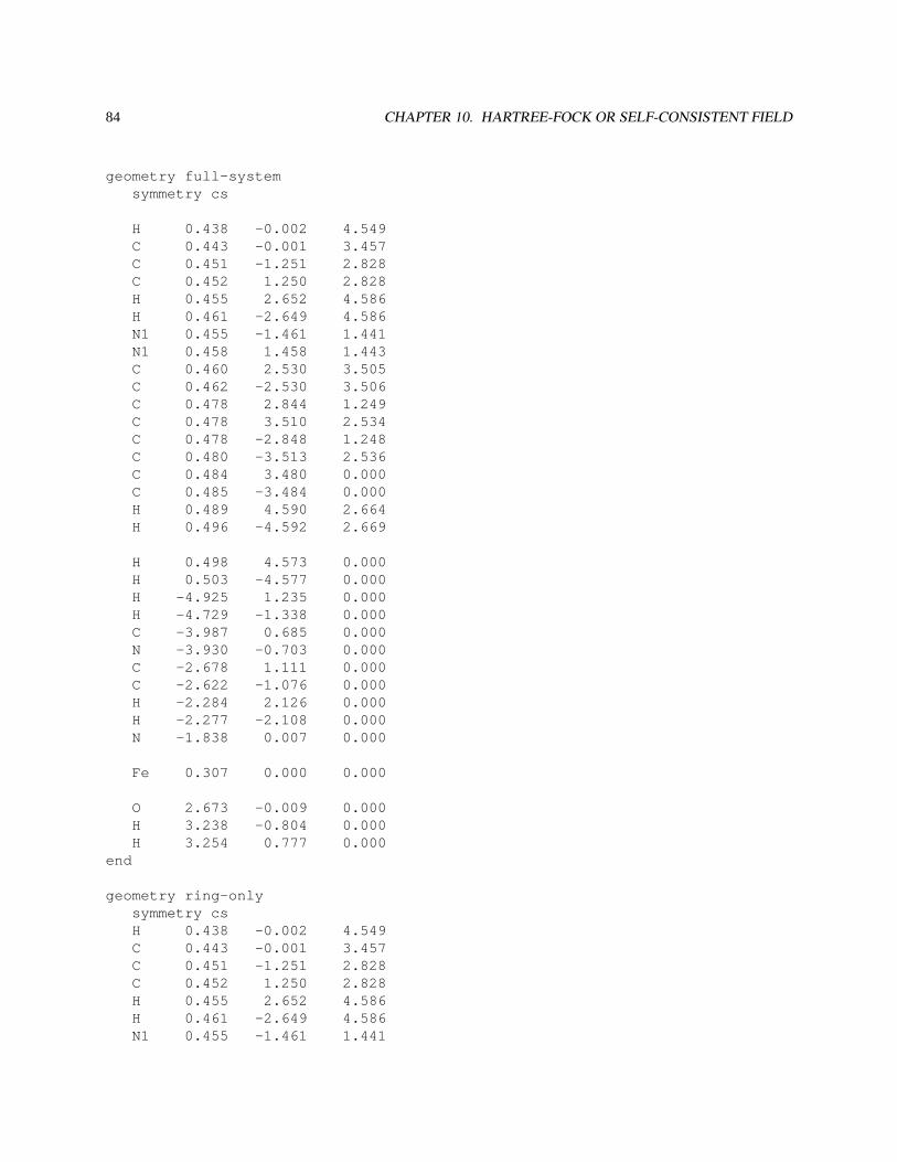
84 CHAPTER 10. HARTREE-FOCK OR SELF-CONSISTENT FIELD
geometry full-systemsymmetry cs
H 0.438 -0.002 4.549C 0.443 -0.001 3.457C 0.451 -1.251 2.828C 0.452 1.250 2.828H 0.455 2.652 4.586H 0.461 -2.649 4.586N1 0.455 -1.461 1.441N1 0.458 1.458 1.443C 0.460 2.530 3.505C 0.462 -2.530 3.506C 0.478 2.844 1.249C 0.478 3.510 2.534C 0.478 -2.848 1.248C 0.480 -3.513 2.536C 0.484 3.480 0.000C 0.485 -3.484 0.000H 0.489 4.590 2.664H 0.496 -4.592 2.669
H 0.498 4.573 0.000H 0.503 -4.577 0.000H -4.925 1.235 0.000H -4.729 -1.338 0.000C -3.987 0.685 0.000N -3.930 -0.703 0.000C -2.678 1.111 0.000C -2.622 -1.076 0.000H -2.284 2.126 0.000H -2.277 -2.108 0.000N -1.838 0.007 0.000
Fe 0.307 0.000 0.000
O 2.673 -0.009 0.000H 3.238 -0.804 0.000H 3.254 0.777 0.000
end
geometry ring-onlysymmetry csH 0.438 -0.002 4.549C 0.443 -0.001 3.457C 0.451 -1.251 2.828C 0.452 1.250 2.828H 0.455 2.652 4.586H 0.461 -2.649 4.586N1 0.455 -1.461 1.441
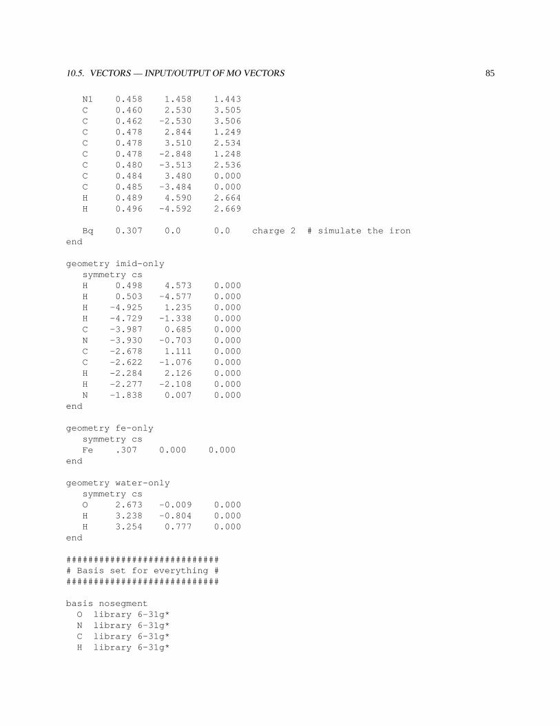
10.5. VECTORS — INPUT/OUTPUT OF MO VECTORS 85
N1 0.458 1.458 1.443C 0.460 2.530 3.505C 0.462 -2.530 3.506C 0.478 2.844 1.249C 0.478 3.510 2.534C 0.478 -2.848 1.248C 0.480 -3.513 2.536C 0.484 3.480 0.000C 0.485 -3.484 0.000H 0.489 4.590 2.664H 0.496 -4.592 2.669
Bq 0.307 0.0 0.0 charge 2 # simulate the ironend
geometry imid-onlysymmetry csH 0.498 4.573 0.000H 0.503 -4.577 0.000H -4.925 1.235 0.000H -4.729 -1.338 0.000C -3.987 0.685 0.000N -3.930 -0.703 0.000C -2.678 1.111 0.000C -2.622 -1.076 0.000H -2.284 2.126 0.000H -2.277 -2.108 0.000N -1.838 0.007 0.000
end
geometry fe-onlysymmetry csFe .307 0.000 0.000
end
geometry water-onlysymmetry csO 2.673 -0.009 0.000H 3.238 -0.804 0.000H 3.254 0.777 0.000
end
############################# Basis set for everything #############################
basis nosegmentO library 6-31g*N library 6-31g*C library 6-31g*H library 6-31g*
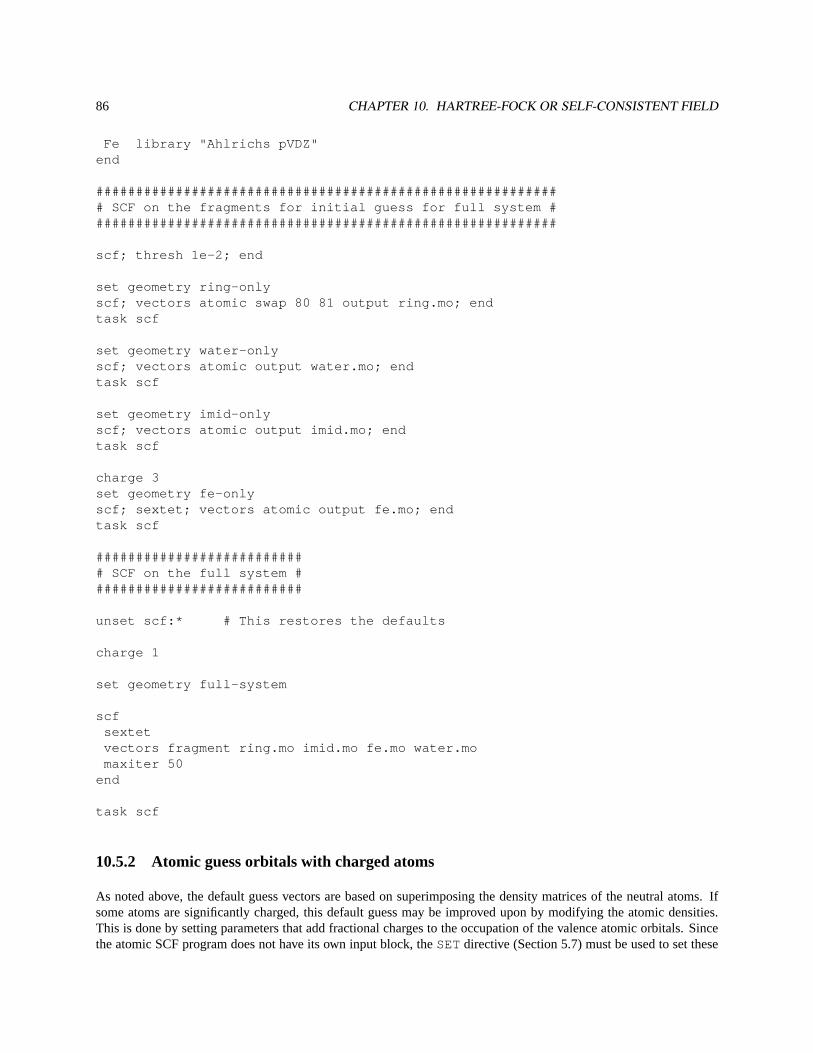
86 CHAPTER 10. HARTREE-FOCK OR SELF-CONSISTENT FIELD
Fe library "Ahlrichs pVDZ"end
########################################################### SCF on the fragments for initial guess for full system ###########################################################
scf; thresh 1e-2; end
set geometry ring-onlyscf; vectors atomic swap 80 81 output ring.mo; endtask scf
set geometry water-onlyscf; vectors atomic output water.mo; endtask scf
set geometry imid-onlyscf; vectors atomic output imid.mo; endtask scf
charge 3set geometry fe-onlyscf; sextet; vectors atomic output fe.mo; endtask scf
########################### SCF on the full system ###########################
unset scf:* # This restores the defaults
charge 1
set geometry full-system
scfsextetvectors fragment ring.mo imid.mo fe.mo water.momaxiter 50
end
task scf
10.5.2 Atomic guess orbitals with charged atoms
As noted above, the default guess vectors are based on superimposing the density matrices of the neutral atoms. Ifsome atoms are significantly charged, this default guess may be improved upon by modifying the atomic densities.This is done by setting parameters that add fractional charges to the occupation of the valence atomic orbitals. Sincethe atomic SCF program does not have its own input block, theSETdirective (Section 5.7) must be used to set these
10.6. ACCURACY OF INITIAL GUESS 87
parameters.
The input specifies a list of tags (i.e., names of atoms in a geometry, see Section 6) and the charges to be added tothose centers. Two parameters must be set as follows:
set atomscf:tags_z <string list_of_tags>set atomscf:z <real list_of_charges>
The array of stringsatomscf:tags_z should be set to the list of tags, and the arrayatomscf:z should be setto the list of charges which must be real numbers (not integers). All atoms that have a tag specified in the list of tagswill be assigned the corresponding charge from the list of charges.
For example, the following specifies that all oxygen atoms with tagObe assigned a charge of-1 and all iron atomswith tagFe be assigned a charge of+2
set atomscf:z -1 2.0set atomscf:tags_z O Fe
There are some limitations to this feature. It is not possible to add electrons to closed shell atoms, nor is it possibleto remove all electrons from a given atom. Attempts to do so will cause the code to report an error, and it will notreport further errors in the input for modifying the charge even when they are detected.
Finally, recall that the database is persistent (Section 3.2) and that the modified settings will be used in subsequentatomic guess calculations unless the data is deleted from the database with theUNSETdirective (Section 5.8).
10.6 Accuracy of initial guess
For SCF, the initial Fock-matrix construction from the atomic guess is now (staring from version 3.3) performed to adefault precision of 1e-7. However, other wavefunctions, notably DFT, use a lower precision. In charged, or diffusebasis sets, this precision may not be sufficient and could result in incorrect ordering of the initial orbitals. The accuracymay be increased with the following directive which should be inserted in the top-level of input (i.e., outside of theSCF input block) and before theTASKdirective.
set tolguess 1e-7
10.7 THRESH — convergence threshold
THRESH <real thresh default 1.0e-4>
This directive specifies the convergence threshold for the calculation. The convergence threshold is the norm ofthe orbital gradient, and has a default value in the code of 10−4.
The norm of the orbital gradient corresponds roughly to the precision available in the wavefunction, and the energyshould be converged to approximately the square of this number. It should be noted, however, that the precision in theenergy will not exceed that of the integral screening tolerance. This tolerance (Section 10.4) is automatically set fromthe convergence threshold, so that sufficient precision is usually available by default.
The default convergence threshold suffices for most SCF energy and geometry optimization calculations, provid-ing about 6–8 decimal places in the energy, and about four significant figures in the density and energy derivative
88 CHAPTER 10. HARTREE-FOCK OR SELF-CONSISTENT FIELD
with respect to nuclear coordinates. However, greater precision may be required for calculations involving weakly in-teracting systems, floppy molecules, finite-difference of gradients to compute the Hessian, and for post-Hartree-Fockcalculations. A threshold of 10−6 is adequate for most such purposes, and a threshold of 10−8 might be necessary forvery high accuracy or very weak interactions. A threshold of 10−10 should be regarded as the best that can be attainedin most circumstances.
10.8 MAXITER — iteration limit
MAXITER <integer maxiter default 8>
The maximum number of iterations for the SCF calculation defaults to 20 for both ROHF/RHF and UHF calcu-lations. For most molecules, this number of iterations is more than sufficient for the quadratically convergent SCFalgorithm to obtain a solution converged to the default threshold (see Section 10.7 above). If the SCF program detectsthat the quadratically convergent algorithm is not efficient, then it will resort to a linearly convergent algorithm andincrease the maximum number of iterations by 10.
Convergence may not be reached in the maximum number of iterations for many reasons, including input error(e.g., an incorrect geometry or a linearly dependent basis), a very low convergence threshold, a poor initial guess, orthe fact that the system is intrinsically hard to converge due to the presence of many states with similar energies.
The following sets the maximum number of SCF iterations to 50:
maxiter 50
10.9 RI-SCF — resolution of the identity approximation
The resolution of the identity (RI) approximation (using the V-approximation of Almlöf and Vahtras) is automaticallyinvoked if a basis set named"riscf basis" is present in the database. This basis will be used as the fitting basis.The RISCF method provides the most computational speedup with the least loss of accuracy when applied to relativelysmall molecules in large basis sets. Calculations on large molecules in modest basis sets will not realize a significantperformance gain from RISCF.
The full RISCF approximation will be applied by default, and theRI-SCF directive serves to modify the extentof the approximation and the computational strategy.
RI-SCF [<string (hessian || preconverge || full) default full>] \[<string (disk || memory || auto) default auto>]
The first three parameters determine the extent of the approximation:
• FULL — is the default and specifies that the RI approximation will be used for all Fock builds in the calculation.This is the fastest of the three options (perhaps 3–10 times faster than direct SCF), but will result in only anapproximate value for the energy.
• HESSIAN — only the orbital Hessian will be calculated with an approximated Fock matrix. This will yieldan exact energy and wavefunction and, using the quadratically convergent SCF algorithm, should result in a1.5–2-fold speedup over direct SCF.
10.10. PROFILE — PERFORMANCE PROFILE 89
• PRECONVERGE— specifies a two-part calculation. First, the SCF calculation is performed with the full RIapproximation. Then an “exact” direct SCF calculation is performed, using the RI approximated Hessian (thesame as theHESSIANoption above). An exact energy and wavefunction will be obtained.
The next three parameters determine the computational strategy:
• AUTO— This is the default option, and allows the code to make its own decision on where to store the 3-centerintegrals. If there is enough memory available, it will use the in-core (memory) option; otherwise, the disk-basedalgorithm will be used, if available.
• MEMORY— This forces storage of the 3-center integrals in memory. If insufficient memory is available, an errorresults.
• DISK — If the ”Disk Resident Array” library is implemented in the local installation of NWChem, the keywordDISK can be used to specify that the 3-center integrals will be stored on disk. Otherwise, an error results.
10.10 PROFILE — performance profile
This directive allows the user to obtain timing and parallel execution information about the SCF module. It is specifiedby the simple keyword
PROFILE
This option can be helpful in understanding the computational performance of an SCF calculation. However, itcan introduce a significant overhead on machines that have expensive timing routines, such as the SUN.
10.11 DIIS — DIIS convergence
This directive allows the user to specify DIIS convergence rather than second-order convergence for the SCF calcula-tion. The form of the directive is as follows:
DIIS
The implementation of this option is currently fairly rudimentary. It does not have level-shifting and damping, anddoes not support open shells or UHF. It is provided on an “as is” basis, and should be used with caution.
When theDIIS directive is specified in the input, the user has the additional option of specifying the size of thesubspace for the DIIS extrapolation. This is accomplished with theDIISBAS directive, which is of the form:
DIISBAS <integer diisbas default 5>
The default of 5 should be adequate for most applications, but may be increased if convergence is poor. On largesystems, it may be necessary to specify a lower value fordiisbas , to conserve memory.

90 CHAPTER 10. HARTREE-FOCK OR SELF-CONSISTENT FIELD
10.12 DIRECT and SEMIDIRECT — recomputation of integrals
In the context of SCF calculations direct means that all integrals are recomputed as required and none are stored.The other extreme are disk- or memory-resident (sometimes termed conventional) calculations in which all integralsare computed once and stored. Semi-direct calculations are between these two extremes with some integrals beingprecomputed and stored, and all other integrals being recomputed as necessary.
The default behavior of the SCF module is
• If enough memory is available, the integrals are computed once and are cached in memory.
• If there is not enough memory to store all the integrals at once, then 95% of the available disk space in thescratch directory (see Section 5.2) is assumed to be available for this purpose, and as many integrals as possibleare cached on disk (with no memory being used for caching). Some attempt is made to store the most expensiveintegrals in the cache.
• If there is not enough room in memory or on disk for all the integrals, then the ones that are not cached arerecomputed in a semidirect fashion.
The integral file is deleted at the end of a calculation, so it is not possible to restart a semidirect calculation whenthe integrals are cached in memory or on disk. Many computer systems (e.g., the EMSL IBM SP) clear the fastscratch space at the end of each job, adding a further complication to the problem of restarting aparallel semidirectcalculation.
On the IBM SP or any other computer with fast disks local to each processor, semidirect calculation offers the bestbehavior. It can result inquadratic speedupas more processors are added.
A fully direct calculation (with recomputation of the integrals at each iteration) is forced by specifying the directive
DIRECT
Alternatively, theSEMIDIRECTdirective can be used to control the default semidirect calculation by defining theamount of disk space and the cache memory size. The form of this directive is as follows:
SEMIDIRECT [filesize <integer filesize default disksize>][memsize <integer memsize default available>][filename <string filename default $file_prefix.aoints$>]
The keywordFILESIZE allows the user to specify the amount of disk space to be used per process for storingthe integrals in 64-bit words. Similarly, the keywordMEMSIZEallows the user to specify the number of 64-bit wordsto be used per process for caching integrals in memory. (Note: If the amount of storage space specified by the entryfor memsize is not available, the code cuts the value in half and checks again for available space. This process isrepeated until the request is satisfied.)
By default, the integral files are placed into the scratch directory (see Section 5.2). Specifying the keywordFILENAMEoverrides this default. The user-specified name entered in the stringfilename has the process numberappended to it, so that each process has a distinct file but with a common base-name and directory. Therefore, it isnot possible to use this keyword to specify different disks for different processes. TheSCRATCH_DIRdirective (seeSection 5.2) can be used for this purpose.
For example, to force full recomputation of all integrals:
direct
10.12. DIRECT AND SEMIDIRECT — RECOMPUTATION OF INTEGRALS 91
Exactly the same result could be obtained by entering the directive:
semidirect filesize 0 memsize 0
To disable the use of memory for caching integrals and limit disk usage by each process to 100 megawords (MW):
semidirect memsize 0 filesize 100000000
The integral records are typically 32769 words long and any non-zero value forfilesize or memsize shouldbe enough to hold at least one record.
10.12.1 Integral File Size and Format for the SCF Module
The file format is rather complex, since it accommodates a variety of packing and compression options and the dis-tribution of data. This section presents some information that may help the user understand the output, and illustrateshow to use the output information to estimate file sizes.
If integrals are stored with a threshold of greater than 10−10, then the integrals are stored in a 32-bit fixed-pointformat (with appropriate treatment for large values to retain precision). If integrals are stored with a threshold lessthan 10−10, however, the values are stored in 64-bit floating-point format. If a replicated-data calculation is being run,then 8 bits are used for each basis function label, unless there are more than 256 functions, in which case 16 bits areused. If distributed data is being used, then the labels are always packed to 8 bits (the distributed blocks always beingless than 256; labels are relative to the start of the block).
Thus, the number (W) of 64-bit words required to storeN integrals, may be computed as
W =
N , 8-bit labels and 32-bit values
32N , 16-bit labels and 32-bit values32N , 8-bit labels and 64-bit values
2N , 16-bit labels and 64-bit values
The actual number of words required can exceed this computed value by up to one percent, due to bookkeepingoverhead, and because the file itself is organized into fixed-size records.
With at least the default print level, all semidirect (not direct) calculations will print out information about theintegral file and the number of integrals computed. The form of this output is as follows:
Integral file = ./c6h6.aoints.0Record size in doubles = 32769 No. of integs per rec = 32768Max. records in memory = 3 Max. records in file = 5No. of bits per label = 8 No. of bits per value = 32
#quartets = 2.0D+04 #integrals = 7.9D+05 direct = 63.6% cached = 36.4%
The file information above relates only to process 0. The line of information about the number of quartets, integrals,etc., is a sum over all processes.
When the integral file is closed, additional information of the following form is printed:
------------------------------------------------------------EAF file 0: "./c6h6.aoints.0" size=262152 bytes
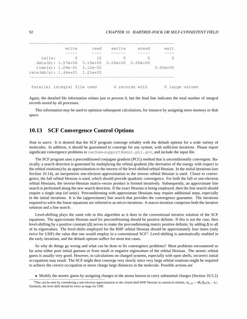
92 CHAPTER 10. HARTREE-FOCK OR SELF-CONSISTENT FIELD
------------------------------------------------------------write read awrite aread wait----- ---- ------ ----- ----
calls: 6 12 0 0 0data(b): 1.57e+06 3.15e+06 0.00e+00 0.00e+00time(s): 1.09e-01 3.12e-02 0.00e+00
rate(mb/s): 1.44e+01 1.01e+02------------------------------------------------------------
Parallel integral file used 4 records with 0 large values
Again, the detailed file information relates just to process 0, but the final line indicates the total number of integralrecords stored by all processes.
This information may be used to optimize subsequent calculations, for instance by assigning more memory or diskspace.
10.13 SCF Convergence Control Options
Note to users:It is desired that the SCF program converge reliably with the default options for a wide variety ofmolecules. In addition, it should be guaranteed to converge for any system, with sufficient iterations. Please reportsignificant convergence problems [email protected] , and include the input file.
The SCF program uses a preconditioned conjugate gradient (PCG) method that is unconditionally convergent. Ba-sically, a search direction is generated by multiplying the orbital gradient (the derivative of the energy with respect tothe orbital rotations) by an approximation to the inverse of the level-shifted orbital Hessian. In the initial iterations (seeSection 10.14), an inexpensive one-electron approximation to the inverse orbital Hessian is used. Closer to conver-gence, the full orbital Hessian is used, which should provide quadratic convergence. For both the full or one-electronorbital Hessians, the inverse-Hessian matrix-vector product is formed iteratively. Subsequently, an approximate linesearch is performed along the new search direction. If the exact Hessian is being employed, then the line search shouldrequire a single step (of unity). Preconditioning with approximate Hessians may require additional steps, especiallyin the initial iterations. It is the (approximate) line search that provides the convergence guarantee. The iterationsrequired to solve the linear equations are referred to as micro-iterations. A macro-iteration comprises both the iterativesolution and a line search.
Level-shifting plays the same role in this algorithm as it does in the conventional iterative solution of the SCFequations. The approximate Hessian used for preconditioning should be positive definite. If this is not the case, thenlevel-shifting by a positive constant (∆) serves to make the preconditioning matrix positive definite, by adding∆ to allof its eigenvalues. The level-shifts employed for the RHF orbital Hessian should be approximately four times (onlytwice for UHF) the value that one would employ in a conventional SCF2. Level-shifting is automatically enabled inthe early iterations, and the default options suffice for most test cases.
So why do things go wrong and what can be done to fix convergence problems? Most problems encountered sofar arise either poor initial guesses or from small or negative eigenvalues of the orbital Hessian. The atomic orbitalguess is usually very good. However, in calculations on charged systems, especially with open shells, incorrect initialoccupations may result. The SCF might then converge very slowly since very large orbital rotations might be requiredto achieve the correct occupation or move charge large distances in the molecule. Possible actions are
• Modify the atomic guess by assigning charges to the atoms known to carry substantial charges (Section 10.5.2)2This can be seen by considering a one-electron approximation to the closed-shell RHF Hessian in canonical orbitals,Aia, jb = 4δi j δab(εa− εi).
Similarly, the level shift should be twice as large for UHF.
10.14. NR — CONTROLLING THE NEWTON-RAPHSON 93
• Examining an analysis of the initial orbitals (Section 10.17) and then swapping them to attain the desired occu-pation (Section 10.5).
• Converging the calculation in a minimial basis set, which is usually easier, and then projecting into a larger basisset (Section 10.5).
• Using the fragment orbital initial guess (Section 10.5.1).
Small or negative Hessian eigenvalues can occur even though the calculation seem to be close to convergence (asmeasured by the gradient norm, or the off-diagonal Fock matrix elements). Small eigenvalues will cause the iterativelinear equation solver to converge slowly, resulting in an excessive number of micro-iterations. This makes the SCFexpensive in terms of computation time, and it is possible to exceed the maximum number of iterations withoutachieving the accuracy required for quadratic convergence — which causes more macro-iterations to be performed.
Two main options are available when a problem will not converge: Newton-Raphson can be disabled temporarilyor permanently (see Section 10.14), and level-shifting can be applied to the matrix (see Section 10.15). In some cases,both options may be necessary to achieve final convergence.
If there is reason to suspect a negative eigenvalue, the first course is to disable the Newton-Raphson iteration untilthe solution is closer to convergence. It may be necessary to disable it completely. At some point close to convergence,the Hessian will be positive definite, so disabling Newton-Raphson should yield a solution with approximately thesame convergence rate as DIIS.
If temporarily disabling Newton-Raphson is not sufficient to achieve convergence, it may be necessary to disableit entirely and apply a small level-shift to the approximate Hessian. This should improve the convergence rate of themicro-iterations and stabilize the macro-iterations. The level-shifting will destroy exact quadratic convergence, butthe optimization process is automatically adjusted to reflect this by enforcing conjugacy and reducing the accuracy towhich the linear equations are solved. The net result of this is that the solution will do more macro-iterations, but eachone should take less time than it would with the unshifted Hessian.
The following sections describe the directives needed to disable the Newton-Raphson iteration and specify level-shifting.
10.14 NR — controlling the Newton-Raphson
NR <real nr_switch default 0.1>
The exact orbital Hessian is adopted as the preconditioner when the maximum element of the orbital gradientis below the value specified fornr_switch . The default value is 0.1, which means that Newton-Raphson will bedisabled until the maximum value of the orbital gradient (twice the largest off-diagonal Fock matrix element) is lessthan 0.1. To disable the Newton-Raphson entirely, the value ofnr_switch must be set to zero. The directive toaccomplish this is as follows:
nr 0
10.15 LEVEL — level-shifting the orbital Hessian
This directive allows the user to specify level-shifting to obtain a positive-definite preconditioning matrix for theSCF solution procedure. Separate level shifts can be set for the first-order convergent one-electron approximation tothe Hessian used with the preconditioned conjugate gradient (PCG) method, and for the full Hessian used with the
94 CHAPTER 10. HARTREE-FOCK OR SELF-CONSISTENT FIELD
Newton-Raphson (NR) approach. It is also possible to change the level-shift automatically as the solution attains somespecified accuracy. The form of the directive is as follows:
LEVEL [pcg <real initial default 20.0> \[<real tol default 0.5> <real final default 0.0>]] \
[nr <real initial default 0.0> \[<real tol default 0.0> <real final default 0.0>]]
This directive contains only two keywords: one for the PCG method and the other for the exact Hessian (NewtonRaphson, or NR). Use of PCG or NR is determined by the input specified fornr_switch on theNRdirective, Section10.14 above.
Specifying the keywordpcg on theLEVELdirective allows the user to define the level shifting for the approximate(i.e., PCG) method. Specifying the keywordnr allows the user to define the level shifting for the exact Hessians. Inboth options, the initial level shift is defined by the value specified for the variableinitial . Optionally,tol can bespecified independently with each keyword to define the level of accuracy that must be attained in the solution beforethe level shifting is changed to the value specified by input in the real variablefinal . Level shifts and gradientthresholds are specified in atomic units.
For the PCG method (as specified using the keywordpcg ), the defaults for this input are 20.0 forinitial , 0.5for tol , and 0.0 forfinal . This means that the approximate Hessian will be shifted by 20.0 until the maximumelement of the gradient falls below 0.5, at which point the shift will be set to zero.
For the exact Hessian (as specified using the keywordnr ), the defaults are all zero. The exact Hessian is usuallynot shifted since this destroys quadratic convergence. An example of an input directive that applies a shift of 0.2 to theexact Hessian is as follows:
level nr 0.2
To apply this shift to the exact Hessian only until the maximum element of the gradient falls below 0.005, therequired input directive is as follows:
level nr 0.2 0.005 0
Note that in both of these examples, the parameters for the PCG method are at the default values. To obtain valuesdifferent from the defaults, the keywordpcg must also be specified. For example, to specify the level shifting in theabove example for the exact Hessianandnon-default shifting for the PCG method, the directive would be somethinglike the following:
level pcg 20 0.3 0.0 nr 0.2 0.005 0.0
This input will cause the PCG method to be level-shifted by 20.0 until the maximum element of the gradient fallsbelow 0.3, then the shift will be zero. For the exact Hessian, the level shifting is initially 0.2, until the maximumelement falls below 0.005, after which the shift is zero.
The default options correspond to
level pcg 20 0.5 0 nr 0 0 0
10.16 Orbtial Localization
The SCF module includes anexperimentalimplementation of orbital localization, including Foster-Boys and Pipek-Mezey which only works for closed-shell (RHF) wavefunctions. There is currently no input in the SCF block to control

10.16. ORBTIAL LOCALIZATION 95
this so theSETdirective (Section 5.7) must be used.
The directive
set scf:localize t
will separately localize the core, valence, and virtual orbital spaces using the Pipek-Mezey algorithm. If the additionaldirective
set scf:loctype FB
is included, then the Foster-boys algorithm is used. The partitioning of core-orbitals is performed using the atomicinformation described in Section 15.1.1.
In the next release, this functionality will be extended to included all wavefunctions using molecular orbitals.

96 CHAPTER 10. HARTREE-FOCK OR SELF-CONSISTENT FIELD
10.17 Printing Information from the SCF Module
All output from the SCF module is controlled using thePRINT directive described in Section 5.6. The following listdescribes the items from SCF that are currently under direct print control, along with the print level for each one.
Name Print Level Description“atomic guess density” debug guess density matrix“atomic scf” debug details of atomic SCF“mo guess” default brief info from mo guess“information” low results“initial vectors” debug“intermediate vectors” debug“final vectors” debug“final vectors analysis” default“initial vectors analysis” never“intermediate evals” debug“final evals” default“schwarz” high integral screening info & stats at completion“screening statistics” debug display stats after every Fock build“geometry” high“symmetry” debug detailed symmetry info“basis” high“geombas” debug detailed basis map info“vectors i/o” default report vectors I/O“parameters” default convergence parameters“convergence” default info each iteration
Table 10.1: SCF Print Control Specifications

10.18. HARTREE-FOCK OR SCF, MCSCF AND MP2 GRADIENTS 97
10.18 Hartree-Fock or SCF, MCSCF and MP2 Gradients
The input for this directive allows the user to adjust the print control for the SCF, UHF, ROHF, MCSCF and MP2gradients. The form of the directive is as follows:
GRADIENTS[print || noprint] ...
END
The complementary keyword pairprint andnoprint allows the user some additional control on the informa-tion that can be included in the print output from the SCF calculation. Currently, only a few items can be explicitlyinvoked via print control. These are as follows:
Name Print Level Description“information” low calculation info“geometry” high geometry information“basis” high basis set(s) used“forces” low details of force components“timing” default timing for each phase
Table 10.2: Gradient Print Control Specifications

98 CHAPTER 10. HARTREE-FOCK OR SELF-CONSISTENT FIELD
Chapter 11
DFT for Molecules (DFT)
The NWChem density functional theory (DFT) module uses the Gaussian basis set approach to compute closed shelland open shell densities and Kohn-Sham orbitals in the:
• local density approximation (LDA),
• non-local density approximation (NLDA),
• local spin-density approximation (LSD),
• non-local spin-density approximation (NLSD), and
• any empirical mixture of local and non-local approximations (including exact exchange).
The formal scaling of the DFT computation can be reduced by choosing to use auxiliary Gaussian basis sets to fitthe charge density (CD) and/or fit the exchange-correlation (XC) potential.
DFT input is provided using the compoundDFTdirective
DFT...
END
The actual DFT calculation will be performed when the input module encounters theTASKdirective (Section 5.10).
TASK DFT
Once a user has specified a geometry and a Kohn-Sham orbital basis set the DFT module can be invoked with noinput directives (defaults invoked throughout). There are sub-directives which allow for customized application; thosecurrently provided as options for the DFT module are:
VECTORS [[input] (<string input_movecs default atomic>) || \(project <string basisname> <string filename>)] \
[swap [alpha||beta] <integer vec1 vec2> ...] \[output <string output_filename default input_movecs>] \[lock]
99
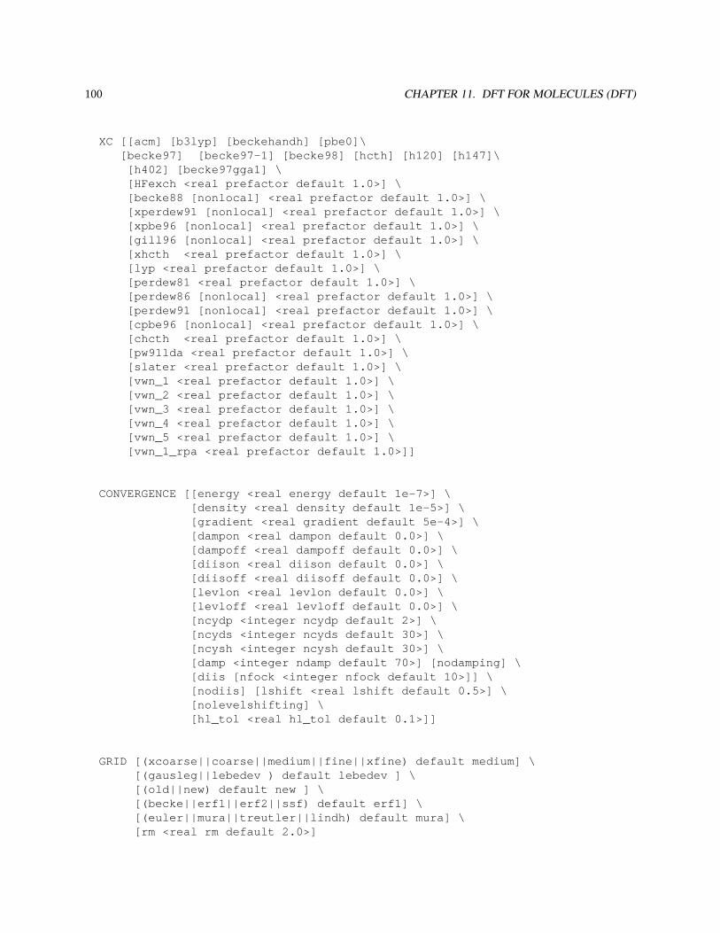
100 CHAPTER 11. DFT FOR MOLECULES (DFT)
XC [[acm] [b3lyp] [beckehandh] [pbe0]\[becke97] [becke97-1] [becke98] [hcth] [h120] [h147]\
[h402] [becke97gga1] \[HFexch <real prefactor default 1.0>] \[becke88 [nonlocal] <real prefactor default 1.0>] \[xperdew91 [nonlocal] <real prefactor default 1.0>] \[xpbe96 [nonlocal] <real prefactor default 1.0>] \[gill96 [nonlocal] <real prefactor default 1.0>] \[xhcth <real prefactor default 1.0>] \[lyp <real prefactor default 1.0>] \[perdew81 <real prefactor default 1.0>] \[perdew86 [nonlocal] <real prefactor default 1.0>] \[perdew91 [nonlocal] <real prefactor default 1.0>] \[cpbe96 [nonlocal] <real prefactor default 1.0>] \[chcth <real prefactor default 1.0>] \[pw91lda <real prefactor default 1.0>] \[slater <real prefactor default 1.0>] \[vwn_1 <real prefactor default 1.0>] \[vwn_2 <real prefactor default 1.0>] \[vwn_3 <real prefactor default 1.0>] \[vwn_4 <real prefactor default 1.0>] \[vwn_5 <real prefactor default 1.0>] \[vwn_1_rpa <real prefactor default 1.0>]]
CONVERGENCE [[energy <real energy default 1e-7>] \[density <real density default 1e-5>] \[gradient <real gradient default 5e-4>] \[dampon <real dampon default 0.0>] \[dampoff <real dampoff default 0.0>] \[diison <real diison default 0.0>] \[diisoff <real diisoff default 0.0>] \[levlon <real levlon default 0.0>] \[levloff <real levloff default 0.0>] \[ncydp <integer ncydp default 2>] \[ncyds <integer ncyds default 30>] \[ncysh <integer ncysh default 30>] \[damp <integer ndamp default 70>] [nodamping] \[diis [nfock <integer nfock default 10>]] \[nodiis] [lshift <real lshift default 0.5>] \[nolevelshifting] \[hl_tol <real hl_tol default 0.1>]]
GRID [(xcoarse||coarse||medium||fine||xfine) default medium] \[(gausleg||lebedev ) default lebedev ] \[(old||new) default new ] \[(becke||erf1||erf2||ssf) default erf1] \[(euler||mura||treutler||lindh) default mura] \[rm <real rm default 2.0>]
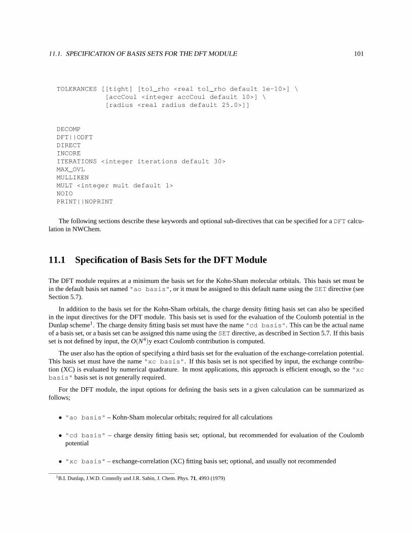
11.1. SPECIFICATION OF BASIS SETS FOR THE DFT MODULE 101
TOLERANCES [[tight] [tol_rho <real tol_rho default 1e-10>] \[accCoul <integer accCoul default 10>] \[radius <real radius default 25.0>]]
DECOMPDFT||ODFTDIRECTINCOREITERATIONS <integer iterations default 30>MAX_OVLMULLIKENMULT <integer mult default 1>NOIOPRINT||NOPRINT
The following sections describe these keywords and optional sub-directives that can be specified for aDFTcalcu-lation in NWChem.
11.1 Specification of Basis Sets for the DFT Module
The DFT module requires at a minimum the basis set for the Kohn-Sham molecular orbitals. This basis set must bein the default basis set named"ao basis" , or it must be assigned to this default name using theSETdirective (seeSection 5.7).
In addition to the basis set for the Kohn-Sham orbitals, the charge density fitting basis set can also be specifiedin the input directives for the DFT module. This basis set is used for the evaluation of the Coulomb potential in theDunlap scheme1. The charge density fitting basis set must have the name"cd basis" . This can be the actual nameof a basis set, or a basis set can be assigned this name using theSETdirective, as described in Section 5.7. If this basisset is not defined by input, theO(N4)y exact Coulomb contribution is computed.
The user also has the option of specifying a third basis set for the evaluation of the exchange-correlation potential.This basis set must have the name"xc basis" . If this basis set is not specified by input, the exchange contribu-tion (XC) is evaluated by numerical quadrature. In most applications, this approach is efficient enough, so the"xcbasis" basis set is not generally required.
For the DFT module, the input options for defining the basis sets in a given calculation can be summarized asfollows;
• "ao basis" – Kohn-Sham molecular orbitals; required for all calculations
• "cd basis" – charge density fitting basis set; optional, but recommended for evaluation of the Coulombpotential
• "xc basis" – exchange-correlation (XC) fitting basis set; optional, and usually not recommended
1B.I. Dunlap, J.W.D. Connolly and J.R. Sabin, J. Chem. Phys.71, 4993 (1979)
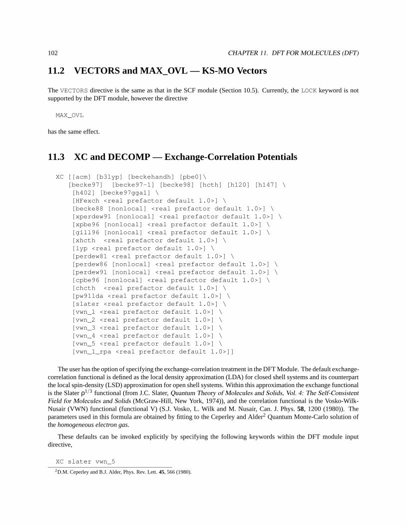
102 CHAPTER 11. DFT FOR MOLECULES (DFT)
11.2 VECTORS and MAX_OVL — KS-MO Vectors
TheVECTORSdirective is the same as that in the SCF module (Section 10.5). Currently, theLOCKkeyword is notsupported by the DFT module, however the directive
MAX_OVL
has the same effect.
11.3 XC and DECOMP — Exchange-Correlation Potentials
XC [[acm] [b3lyp] [beckehandh] [pbe0]\[becke97] [becke97-1] [becke98] [hcth] [h120] [h147] \
[h402] [becke97gga1] \[HFexch <real prefactor default 1.0>] \[becke88 [nonlocal] <real prefactor default 1.0>] \[xperdew91 [nonlocal] <real prefactor default 1.0>] \[xpbe96 [nonlocal] <real prefactor default 1.0>] \[gill96 [nonlocal] <real prefactor default 1.0>] \[xhcth <real prefactor default 1.0>] \[lyp <real prefactor default 1.0>] \[perdew81 <real prefactor default 1.0>] \[perdew86 [nonlocal] <real prefactor default 1.0>] \[perdew91 [nonlocal] <real prefactor default 1.0>] \[cpbe96 [nonlocal] <real prefactor default 1.0>] \[chcth <real prefactor default 1.0>] \[pw91lda <real prefactor default 1.0>] \[slater <real prefactor default 1.0>] \[vwn_1 <real prefactor default 1.0>] \[vwn_2 <real prefactor default 1.0>] \[vwn_3 <real prefactor default 1.0>] \[vwn_4 <real prefactor default 1.0>] \[vwn_5 <real prefactor default 1.0>] \[vwn_1_rpa <real prefactor default 1.0>]]
The user has the option of specifying the exchange-correlation treatment in the DFT Module. The default exchange-correlation functional is defined as the local density approximation (LDA) for closed shell systems and its counterpartthe local spin-density (LSD) approximation for open shell systems. Within this approximation the exchange functionalis the Slaterρ1/3 functional (from J.C. Slater,Quantum Theory of Molecules and Solids, Vol. 4: The Self-ConsistentField for Molecules and Solids (McGraw-Hill, New York, 1974)), and the correlation functional is the Vosko-Wilk-Nusair (VWN) functional (functional V) (S.J. Vosko, L. Wilk and M. Nusair, Can. J. Phys.58, 1200 (1980)). Theparameters used in this formula are obtained by fitting to the Ceperley and Alder2 Quantum Monte-Carlo solution ofthehomogeneous electron gas.
These defaults can be invoked explicitly by specifying the following keywords within the DFT module inputdirective,
XC slater vwn_52D.M. Ceperley and B.J. Alder, Phys. Rev. Lett.45, 566 (1980).
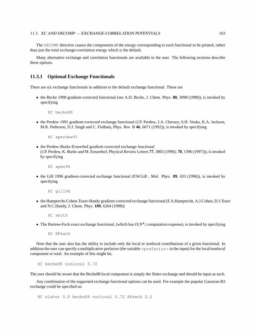
11.3. XC AND DECOMP — EXCHANGE-CORRELATION POTENTIALS 103
TheDECOMPdirective causes the components of the energy corresponding to each functional to be printed, ratherthan just the total exchange-correlation energy which is the default.
Many alternative exchange and correlation functionals are available to the user. The following sections describethese options.
11.3.1 Optional Exchange Functionals
There are six exchange functionals in addition to the default exchange functional. These are
• the Becke 1998 gradient-corrected functional (see A.D. Becke, J. Chem. Phys.88, 3098 (1988)), is invoked byspecifying
XC becke88
• the Perdew 1991 gradient-corrected exchange functional (J.P. Perdew, J.A. Chevary, S.H. Vosko, K.A. Jackson,M.R. Pederson, D.J. Singh and C. Fiolhais, Phys. Rev. B46, 6671 (1992)), is invoked by specifying
XC xperdew91
• the Perdew-Burke-Ernzerhof gradient-corrected exchange functional(J.P. Perdew, K. Burke and M. Ernzerhof, Physical Review Letters77, 3865 (1996);78, 1396 (1997))), is invokedby specifying
XC xpbe96
• the Gill 1996 gradient-corrected exchange functional (P.W.Gill , Mol. Phys.89, 433 (1996)), is invoked byspecifying
XC gill96
• the Hamprecht-Cohen-Tozer-Handy gradient-corrected exchange functional (F.A.Hamprecht, A.J.Cohen, D.J.Tozerand N.C.Handy, J. Chem. Phys.109, 6264 (1998))
XC xhcth
• The Hartree-Fock exact exchange functional, (which hasO(N4) computation expense), is invoked by specifying
XC HFexch
Note that the user also has the ability to include only the local or nonlocal contributions of a given functional. Inaddition the user can specify a multiplicative prefactor (the variable<prefactor> in the input) for the local/nonlocalcomponent or total. An example of this might be,
XC becke88 nonlocal 0.72
The user should be aware that the Becke88 local component is simply the Slater exchange and should be input as such.
Any combination of the supported exchange functional options can be used. For example the popular Gaussian B3exchange could be specified as:
XC slater 0.8 becke88 nonlocal 0.72 HFexch 0.2
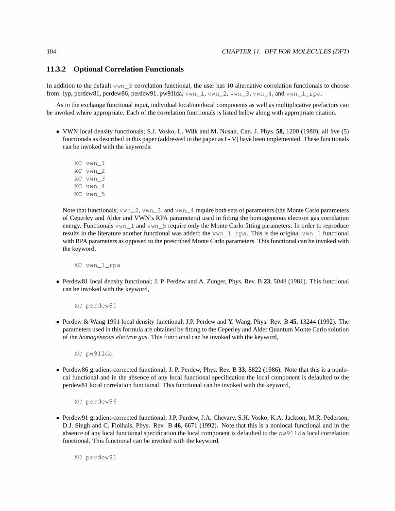
104 CHAPTER 11. DFT FOR MOLECULES (DFT)
11.3.2 Optional Correlation Functionals
In addition to the defaultvwn_5 correlation functional, the user has 10 alternative correlation functionals to choosefrom: lyp, perdew81, perdew86, perdew91, pw91lda,vwn_1 , vwn_2 , vwn_3 , vwn_4 , andvwn_1_rpa .
As in the exchange functional input, individual local/nonlocal components as well as multiplicative prefactors canbe invoked where appropriate. Each of the correlation functionals is listed below along with appropriate citation.
• VWN local density functionals; S.J. Vosko, L. Wilk and M. Nusair, Can. J. Phys.58, 1200 (1980); all five (5)functionals as described in this paper (addressed in the paper as I - V) have been implemented. These functionalscan be invoked with the keywords:
XC vwn_1XC vwn_2XC vwn_3XC vwn_4XC vwn_5
Note that functionals;vwn_2 , vwn_3 , andvwn_4 require both sets of parameters (the Monte Carlo parametersof Ceperley and Alder and VWN’s RPA parameters) used in fitting the homogeneous electron gas correlationenergy. Functionalsvwn_1 andvwn_5 require only the Monte Carlo fitting parameters. In order to reproduceresults in the literature another functional was added; thevwn_1_rpa . This is the originalvwn_1 functionalwith RPA parameters as opposed to the prescribed Monte Carlo parameters. This functional can be invoked withthe keyword,
XC vwn_1_rpa
• Perdew81 local density functional; J. P. Perdew and A. Zunger, Phys. Rev. B23, 5048 (1981). This functionalcan be invoked with the keyword,
XC perdew81
• Perdew & Wang 1991 local density functional; J.P. Perdew and Y. Wang, Phys. Rev. B45, 13244 (1992). Theparameters used in this formula are obtained by fitting to the Ceperley and Alder Quantum Monte Carlo solutionof thehomogeneous electron gas. This functional can be invoked with the keyword,
XC pw91lda
• Perdew86 gradient-corrected functional; J. P. Perdew, Phys. Rev. B33, 8822 (1986). Note that this is a nonlo-cal functional and in the absence of any local functional specification the local component is defaulted to theperdew81 local correlation functional. This functional can be invoked with the keyword,
XC perdew86
• Perdew91 gradient-corrected functional; J.P. Perdew, J.A. Chevary, S.H. Vosko, K.A. Jackson, M.R. Pederson,D.J. Singh and C. Fiolhais, Phys. Rev. B46, 6671 (1992). Note that this is a nonlocal functional and in theabsence of any local functional specification the local component is defaulted to thepw91lda local correlationfunctional. This functional can be invoked with the keyword,
XC perdew91
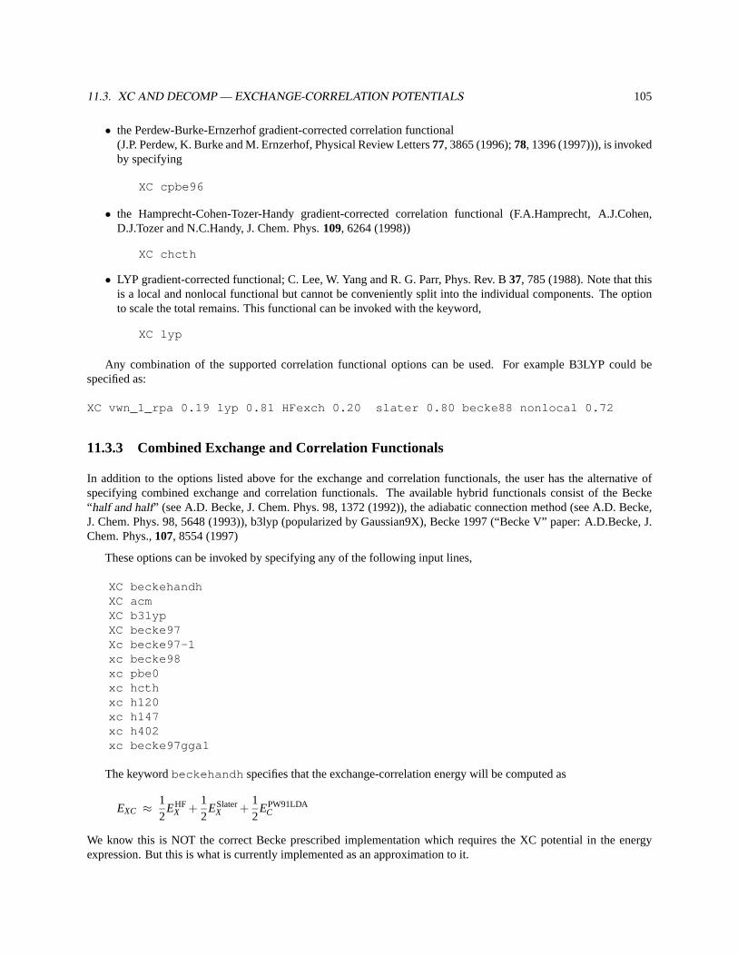
11.3. XC AND DECOMP — EXCHANGE-CORRELATION POTENTIALS 105
• the Perdew-Burke-Ernzerhof gradient-corrected correlation functional(J.P. Perdew, K. Burke and M. Ernzerhof, Physical Review Letters77, 3865 (1996);78, 1396 (1997))), is invokedby specifying
XC cpbe96
• the Hamprecht-Cohen-Tozer-Handy gradient-corrected correlation functional (F.A.Hamprecht, A.J.Cohen,D.J.Tozer and N.C.Handy, J. Chem. Phys.109, 6264 (1998))
XC chcth
• LYP gradient-corrected functional; C. Lee, W. Yang and R. G. Parr, Phys. Rev. B37, 785 (1988). Note that thisis a local and nonlocal functional but cannot be conveniently split into the individual components. The optionto scale the total remains. This functional can be invoked with the keyword,
XC lyp
Any combination of the supported correlation functional options can be used. For example B3LYP could bespecified as:
XC vwn_1_rpa 0.19 lyp 0.81 HFexch 0.20 slater 0.80 becke88 nonlocal 0.72
11.3.3 Combined Exchange and Correlation Functionals
In addition to the options listed above for the exchange and correlation functionals, the user has the alternative ofspecifying combined exchange and correlation functionals. The available hybrid functionals consist of the Becke“half and half” (see A.D. Becke, J. Chem. Phys. 98, 1372 (1992)), the adiabatic connection method (see A.D. Becke,J. Chem. Phys. 98, 5648 (1993)), b3lyp (popularized by Gaussian9X), Becke 1997 (“Becke V” paper: A.D.Becke, J.Chem. Phys.,107, 8554 (1997)
These options can be invoked by specifying any of the following input lines,
XC beckehandhXC acmXC b3lypXC becke97Xc becke97-1xc becke98xc pbe0xc hcthxc h120xc h147xc h402xc becke97gga1
The keywordbeckehandh specifies that the exchange-correlation energy will be computed as
EXC ≈12
EHFX +
12
ESlaterX +
12
EPW91LDAC
We know this is NOT the correct Becke prescribed implementation which requires the XC potential in the energyexpression. But this is what is currently implemented as an approximation to it.
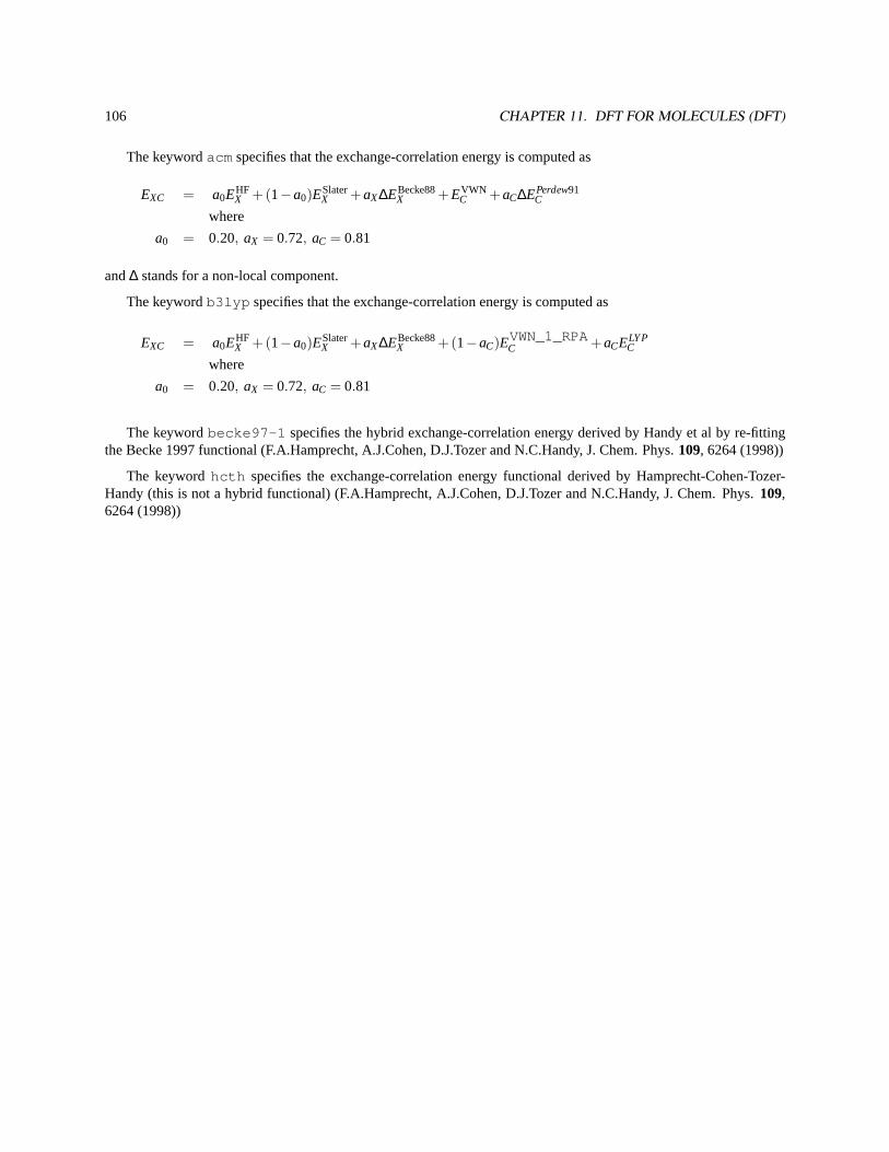
106 CHAPTER 11. DFT FOR MOLECULES (DFT)
The keywordacm specifies that the exchange-correlation energy is computed as
EXC = a0EHFX +(1−a0)ESlater
X +aX∆EBecke88X +EVWN
C +aC∆EPerdew91C
where
a0 = 0.20, aX = 0.72, aC = 0.81
and∆ stands for a non-local component.
The keywordb3lyp specifies that the exchange-correlation energy is computed as
EXC = a0EHFX +(1−a0)ESlater
X +aX∆EBecke88X +(1−aC)EVWN_1_RPA
C +aCELYPC
where
a0 = 0.20, aX = 0.72, aC = 0.81
The keywordbecke97-1 specifies the hybrid exchange-correlation energy derived by Handy et al by re-fittingthe Becke 1997 functional (F.A.Hamprecht, A.J.Cohen, D.J.Tozer and N.C.Handy, J. Chem. Phys.109, 6264 (1998))
The keywordhcth specifies the exchange-correlation energy functional derived by Hamprecht-Cohen-Tozer-Handy (this is not a hybrid functional) (F.A.Hamprecht, A.J.Cohen, D.J.Tozer and N.C.Handy, J. Chem. Phys.109,6264 (1998))
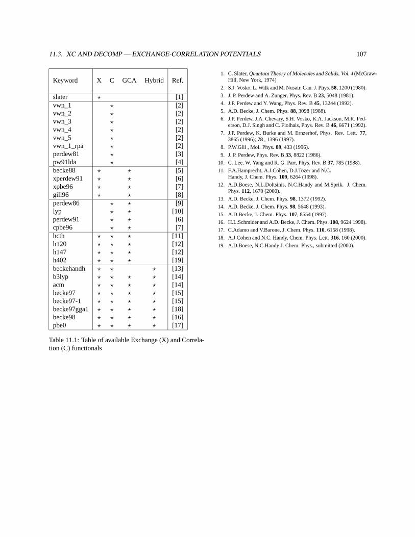
11.3. XC AND DECOMP — EXCHANGE-CORRELATION POTENTIALS 107
Keyword X C GCA Hybrid Ref.
slater ? [1]vwn_1 ? [2]vwn_2 ? [2]vwn_3 ? [2]vwn_4 ? [2]vwn_5 ? [2]vwn_1_rpa ? [2]perdew81 ? [3]pw91lda ? [4]becke88 ? ? [5]xperdew91 ? ? [6]xpbe96 ? ? [7]gill96 ? ? [8]perdew86 ? ? [9]lyp ? ? [10]perdew91 ? ? [6]cpbe96 ? ? [7]hcth ? ? ? [11]h120 ? ? ? [12]h147 ? ? ? [12]h402 ? ? ? [19]beckehandh ? ? ? [13]b3lyp ? ? ? ? [14]acm ? ? ? ? [14]becke97 ? ? ? ? [15]becke97-1 ? ? ? ? [15]becke97gga1 ? ? ? ? [18]becke98 ? ? ? ? [16]pbe0 ? ? ? ? [17]
Table 11.1: Table of available Exchange (X) and Correla-tion (C) functionals
1. C. Slater,Quantum Theory of Molecules and Solids, Vol. 4 (McGraw-Hill, New York, 1974)
2. S.J. Vosko, L. Wilk and M. Nusair, Can. J. Phys.58, 1200 (1980).
3. J. P. Perdew and A. Zunger, Phys. Rev. B23, 5048 (1981).
4. J.P. Perdew and Y. Wang, Phys. Rev. B45, 13244 (1992).
5. A.D. Becke, J. Chem. Phys.88, 3098 (1988).
6. J.P. Perdew, J.A. Chevary, S.H. Vosko, K.A. Jackson, M.R. Ped-erson, D.J. Singh and C. Fiolhais, Phys. Rev. B46, 6671 (1992).
7. J.P. Perdew, K. Burke and M. Ernzerhof, Phys. Rev. Lett.77,3865 (1996);78 , 1396 (1997).
8. P.W.Gill , Mol. Phys.89, 433 (1996).
9. J. P. Perdew, Phys. Rev. B33, 8822 (1986).
10. C. Lee, W. Yang and R. G. Parr, Phys. Rev. B37, 785 (1988).
11. F.A.Hamprecht, A.J.Cohen, D.J.Tozer and N.C.Handy, J. Chem. Phys.109, 6264 (1998).
12. A.D.Boese, N.L.Doltsinis, N.C.Handy and M.Sprik. J. Chem.Phys.112, 1670 (2000).
13. A.D. Becke, J. Chem. Phys.98, 1372 (1992).
14. A.D. Becke, J. Chem. Phys.98, 5648 (1993).
15. A.D.Becke, J. Chem. Phys.107, 8554 (1997).
16. H.L.Schmider and A.D. Becke, J. Chem. Phys.108, 9624 1998).
17. C.Adamo and V.Barone, J. Chem. Phys.110, 6158 (1998).
18. A.J.Cohen and N.C. Handy, Chem. Phys. Lett.316, 160 (2000).
19. A.D.Boese, N.C.Handy J. Chem. Phys., submitted (2000).
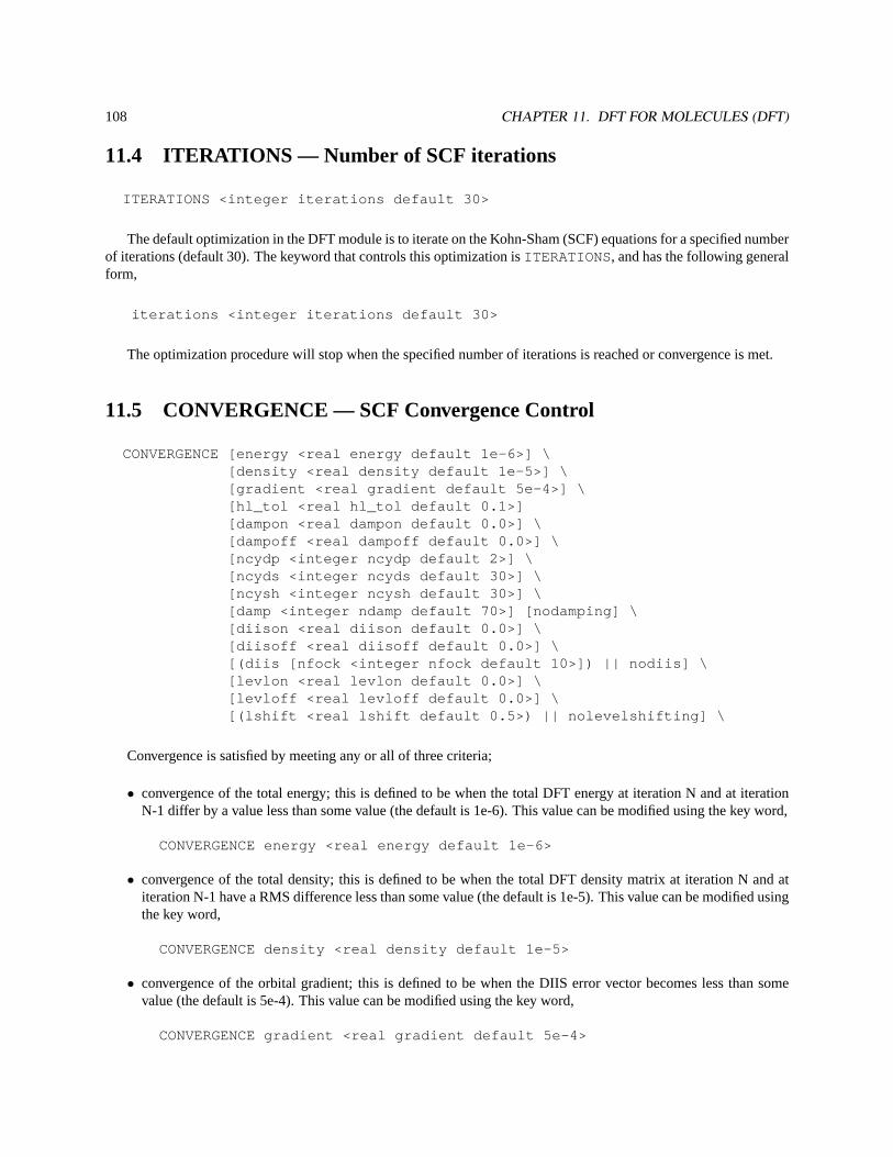
108 CHAPTER 11. DFT FOR MOLECULES (DFT)
11.4 ITERATIONS — Number of SCF iterations
ITERATIONS <integer iterations default 30>
The default optimization in the DFT module is to iterate on the Kohn-Sham (SCF) equations for a specified numberof iterations (default 30). The keyword that controls this optimization isITERATIONS, and has the following generalform,
iterations <integer iterations default 30>
The optimization procedure will stop when the specified number of iterations is reached or convergence is met.
11.5 CONVERGENCE — SCF Convergence Control
CONVERGENCE [energy <real energy default 1e-6>] \[density <real density default 1e-5>] \[gradient <real gradient default 5e-4>] \[hl_tol <real hl_tol default 0.1>][dampon <real dampon default 0.0>] \[dampoff <real dampoff default 0.0>] \[ncydp <integer ncydp default 2>] \[ncyds <integer ncyds default 30>] \[ncysh <integer ncysh default 30>] \[damp <integer ndamp default 70>] [nodamping] \[diison <real diison default 0.0>] \[diisoff <real diisoff default 0.0>] \[(diis [nfock <integer nfock default 10>]) || nodiis] \[levlon <real levlon default 0.0>] \[levloff <real levloff default 0.0>] \[(lshift <real lshift default 0.5>) || nolevelshifting] \
Convergence is satisfied by meeting any or all of three criteria;
• convergence of the total energy; this is defined to be when the total DFT energy at iteration N and at iterationN-1 differ by a value less than some value (the default is 1e-6). This value can be modified using the key word,
CONVERGENCE energy <real energy default 1e-6>
• convergence of the total density; this is defined to be when the total DFT density matrix at iteration N and atiteration N-1 have a RMS difference less than some value (the default is 1e-5). This value can be modified usingthe key word,
CONVERGENCE density <real density default 1e-5>
• convergence of the orbital gradient; this is defined to be when the DIIS error vector becomes less than somevalue (the default is 5e-4). This value can be modified using the key word,
CONVERGENCE gradient <real gradient default 5e-4>
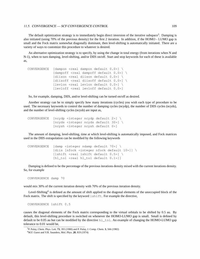
11.5. CONVERGENCE — SCF CONVERGENCE CONTROL 109
The default optimization strategy is to immediately begin direct inversion of the iterative subspace3. Damping isalso initiated (using 70% of the previous density) for the first 2 iteration. In addition, if the HOMO - LUMO gap issmall and the Fock matrix somewhat diagonally dominant, then level-shifting is automatically initiated. There are avariety of ways to customize this procedure to whatever is desired.
An alternative optimization strategy is to specify, by using the change in total energy (from iterations when N andN-1), when to turn damping, level-shifting, and/or DIIS on/off. Start and stop keywords for each of these is availableas,
CONVERGENCE [dampon <real dampon default 0.0>] \[dampoff <real dampoff default 0.0>] \[diison <real diison default 0.0>] \[diisoff <real diisoff default 0.0>] \[levlon <real levlon default 0.0>] \[levloff <real levloff default 0.0>]
So, for example, damping, DIIS, and/or level-shifting can be turned on/off as desired.
Another strategy can be to simply specify how many iterations (cycles) you wish each type of procedure to beused. The necessary keywords to control the number of damping cycles (ncydp), the number of DIIS cycles (ncyds),and the number of level-shifting cycles (ncysh) are input as,
CONVERGENCE [ncydp <integer ncydp default 2>] \[ncyds <integer ncyds default 30>] \[ncysh <integer ncysh default 0>]
The amount of damping, level-shifting, time at which level-shifting is automatically imposed, and Fock matricesused in the DIIS extrapolation can be modified by the following keywords
CONVERGENCE [damp <integer ndamp default 70>] \[diis [nfock <integer nfock default 10>]] \[lshift <real lshift default 0.5>] \[hl_tol <real hl_tol default 0.1>]]
Damping is defined to be the percentage of the previous iterations density mixed with the current iterations density.So, for example
CONVERGENCE damp 70
would mix 30% of the current iteration density with 70% of the previous iteration density.
Level-Shifting4 is defined as the amount of shift applied to the diagonal elements of the unoccupied block of theFock matrix. The shift is specified by the keywordlshift . For example the directive,
CONVERGENCE lshift 0.5
causes the diagonal elements of the Fock matrix corresponding to the virtual orbitals to be shifted by 0.5 au. Bydefault, this level-shifting procedure is switched on whenever the HOMO-LUMO gap is small. Small is defined bydefault to be 0.05 au but can be modified by the directivehl_tol . An example of changing the HOMO-LUMO gaptolerance to 0.01 would be,
3P. Pulay, Chem. Phys. Lett.73, 393 (1980) and P. Pulay, J. Comp. Chem.3, 566 (1982)4M.F. Guest and V.R. Saunders, Mol. Phys.28, 819 (1974)
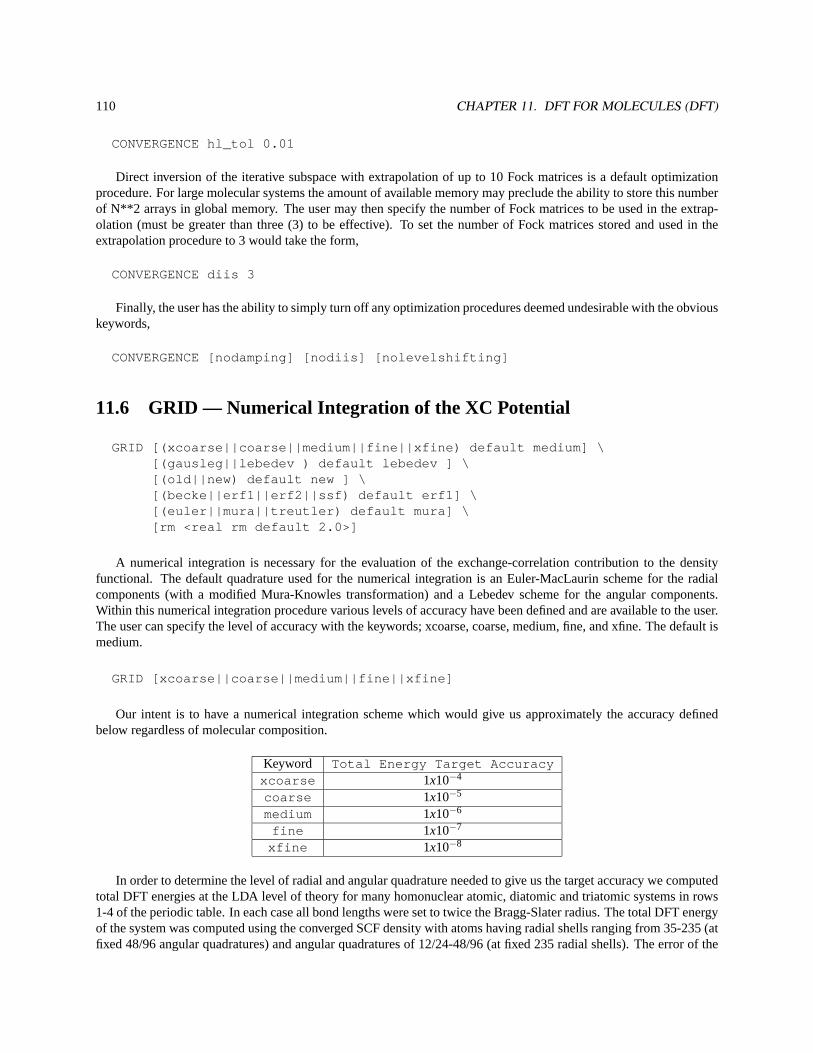
110 CHAPTER 11. DFT FOR MOLECULES (DFT)
CONVERGENCE hl_tol 0.01
Direct inversion of the iterative subspace with extrapolation of up to 10 Fock matrices is a default optimizationprocedure. For large molecular systems the amount of available memory may preclude the ability to store this numberof N**2 arrays in global memory. The user may then specify the number of Fock matrices to be used in the extrap-olation (must be greater than three (3) to be effective). To set the number of Fock matrices stored and used in theextrapolation procedure to 3 would take the form,
CONVERGENCE diis 3
Finally, the user has the ability to simply turn off any optimization procedures deemed undesirable with the obviouskeywords,
CONVERGENCE [nodamping] [nodiis] [nolevelshifting]
11.6 GRID — Numerical Integration of the XC Potential
GRID [(xcoarse||coarse||medium||fine||xfine) default medium] \[(gausleg||lebedev ) default lebedev ] \[(old||new) default new ] \[(becke||erf1||erf2||ssf) default erf1] \[(euler||mura||treutler) default mura] \[rm <real rm default 2.0>]
A numerical integration is necessary for the evaluation of the exchange-correlation contribution to the densityfunctional. The default quadrature used for the numerical integration is an Euler-MacLaurin scheme for the radialcomponents (with a modified Mura-Knowles transformation) and a Lebedev scheme for the angular components.Within this numerical integration procedure various levels of accuracy have been defined and are available to the user.The user can specify the level of accuracy with the keywords; xcoarse, coarse, medium, fine, and xfine. The default ismedium.
GRID [xcoarse||coarse||medium||fine||xfine]
Our intent is to have a numerical integration scheme which would give us approximately the accuracy definedbelow regardless of molecular composition.
Keyword Total Energy Target Accuracyxcoarse 1x10⁻⁴
coarse 1x10⁻⁵
medium 1x10⁻⁶
fine 1x10⁻⁷
xfine 1x10⁻⁸
In order to determine the level of radial and angular quadrature needed to give us the target accuracy we computedtotal DFT energies at the LDA level of theory for many homonuclear atomic, diatomic and triatomic systems in rows1-4 of the periodic table. In each case all bond lengths were set to twice the Bragg-Slater radius. The total DFT energyof the system was computed using the converged SCF density with atoms having radial shells ranging from 35-235 (atfixed 48/96 angular quadratures) and angular quadratures of 12/24-48/96 (at fixed 235 radial shells). The error of the
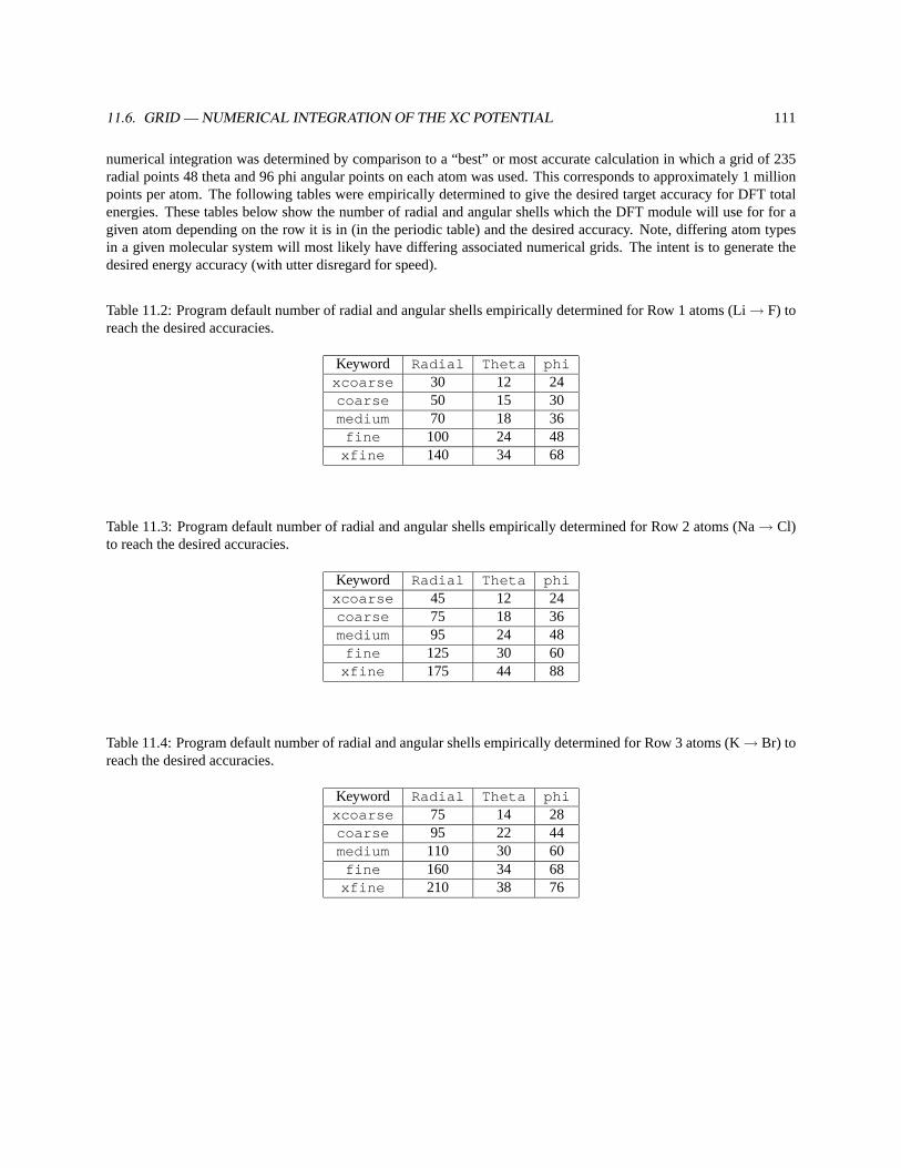
11.6. GRID — NUMERICAL INTEGRATION OF THE XC POTENTIAL 111
numerical integration was determined by comparison to a “best” or most accurate calculation in which a grid of 235radial points 48 theta and 96 phi angular points on each atom was used. This corresponds to approximately 1 millionpoints per atom. The following tables were empirically determined to give the desired target accuracy for DFT totalenergies. These tables below show the number of radial and angular shells which the DFT module will use for for agiven atom depending on the row it is in (in the periodic table) and the desired accuracy. Note, differing atom typesin a given molecular system will most likely have differing associated numerical grids. The intent is to generate thedesired energy accuracy (with utter disregard for speed).
Table 11.2: Program default number of radial and angular shells empirically determined for Row 1 atoms (Li→ F) toreach the desired accuracies.
Keyword Radial Theta phixcoarse 30 12 24coarse 50 15 30medium 70 18 36
fine 100 24 48xfine 140 34 68
Table 11.3: Program default number of radial and angular shells empirically determined for Row 2 atoms (Na→ Cl)to reach the desired accuracies.
Keyword Radial Theta phixcoarse 45 12 24coarse 75 18 36medium 95 24 48
fine 125 30 60xfine 175 44 88
Table 11.4: Program default number of radial and angular shells empirically determined for Row 3 atoms (K→ Br) toreach the desired accuracies.
Keyword Radial Theta phixcoarse 75 14 28coarse 95 22 44medium 110 30 60
fine 160 34 68xfine 210 38 76

112 CHAPTER 11. DFT FOR MOLECULES (DFT)
Table 11.5: Program default number of radial and angular shells empirically determined for Row 4 atoms (Rb→ I) toreach the desired accuracies.
Keyword Radial Theta phixcoarse 105 16 32coarse 130 20 40medium 155 32 64
fine 205 44 88xfine 235 48 96
11.6. GRID — NUMERICAL INTEGRATION OF THE XC POTENTIAL 113
11.6.1 Angular grids
In addition to the simple keyword specifying the desired accuracy as described above, the user has the option ofspecifying a custom quadrature of this type in which ALL atoms have the same grid specification. This is accomplishedby using thegausleg keyword.
Gauss-Legendre angular grid
GRID gausleg <integer nradpts default 50> <integer nagrid default 10>
In this type of grid, the number of phi points is twice the number of theta points. So, for example, a specificationof,
GRID gausleg 80 20
would be interpreted as 80 radial points, 20 theta points, and 40 phi points per center (or 64000 points per center beforepruning).
Lebedev angular grid A second quadrature is the Lebedev scheme for the angular components5. Within this nu-merical integration procedure various levels of accuracy have also been defined and are available to the user. The inputfor this type of grid takes the form,
GRID lebedev <integer radpts > <integer iangquad >
In this context the variable iangquad specifies a certain number of angular points as indicated by the table below.6
Therefore the user can specify any number of radial points along with the level of angular quadrature (1-29).
The user can also specify grid parameters specific for a given atom type: parameters that must be supplied are:atom tag, number of radial points, number of angular points andaccQrad (all three parameters must be given). Asan example, here is a grid input line for the water molecule
grid lebedev 80 11 H 70 8 12 O 90 11 15
5The subroutine for the Lebedev grid was derived from a routine supplied by M. Causà of the University of Torino and from the grid pointssupplied by D.N. Laikov from Moscow State University.
6 V.I. Lebedev and D.N. Laikov, Doklady Mathematics366, 741 (1999).
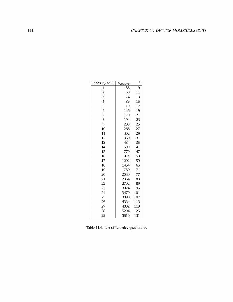
114 CHAPTER 11. DFT FOR MOLECULES (DFT)
IANGQUAD Nangular l1 38 92 50 113 74 134 86 155 110 176 146 197 170 218 194 239 230 2510 266 2711 302 2912 350 3113 434 3514 590 4115 770 4716 974 5317 1202 5918 1454 6519 1730 7120 2030 7721 2354 8322 2702 8923 3074 9524 3470 10125 3890 10726 4334 11327 4802 11928 5294 12529 5810 131
Table 11.6: List of Lebedev quadratures
11.6. GRID — NUMERICAL INTEGRATION OF THE XC POTENTIAL 115
11.6.2 Partitioning functions
GRID [(becke||erf1||erf2||ssf) default erf1]
becke A. D. Becke, J. Chem. Phys.88, 1053 (1988).
ssf R.E.Stratmann, G.Scuseria and M.J.Frisch, Chem. Phys. Lett.257, 213 (1996).
erf1 modified ssf
erf2 modified ssf
Erfn partionioning functions
wA(r) = ∏B6=A
12
[1 − er f(µ′AB)
]µ′AB =
1α
µAB
(1−µ2AB)n
µAB =rA− rB
|rA− rB|
11.6.3 Radial grids
GRID [[euler||mura||treutler] default mura]
euler Euler-McLaurin quadrature wih the transformation devised by C.W. Murray, N.C. Handy, and G.L. Laming,Mol. Phys.78, 997 (1993).
mura Modification of the Murray-Handy-Laming scheme by M.E.Mura and P.J.Knowles, J Chem Phys104, 9848(1996) (we are not using the scaling factors proposed in this paper).
treutler Gauss-Chebyshev using the transformation suggested by O.Treutler and R.Alrhichs, J.Chem.Phys102,346 (1995).
11.6.4 Grid Scheme
GRID [[old||new] default new]
In Nwchem 4.0 the XC integration code has been re-written using a space decomposiition scheme similar to theone proposed in R.E.Stratmann, G.Scuseria and M.J.Frisch, Chem. Phys. Lett.257, 213 (1996) (keywordnew).
To use the XC integration routines available in older version of NWChem, use the keywordold .
116 CHAPTER 11. DFT FOR MOLECULES (DFT)
11.7 TOLERANCES — Screening tolerances
TOLERANCES [[tight] [tol_rho <real tol_rho default 1e-10>] \[accCoul <integer accCoul default 10>] \[radius <real radius default 25.0>]]
The user has the option of controlling screening for the tolerances in the integral evaluations for the DFT module. Inmost applications, the default values will be adequate for the calculation, but different values can be specified in theinput for the DFT module using the keywords described below.
The input parameteraccCoul is used to define the tolerance in Schwarz screening for the Coulomb integrals.Only integrals with estimated values greater than 10(−accCoul) are evaluated.
TOLERANCES accCoul <integer accCoul default 10>
Screening away needless computation of the XC functional (on the grid) due to negligible density is also possiblewith the use of,
TOLERANCES tol_rho <real tol_rho default 1e-10>
XC functional computation is bypassed if the corresponding density elements are less thantol_rho .
A screening parameter,radius , used in the screening of the Becke or Delley spatial weights is also available as,
TOLERANCES radius <real radius default 25.0>
where radius is the cutoff value in bohr.
The tolerances as discussed previously are insured at convergence. More sleazy tolerances are invoked early inthe iterative process which can speed things up a bit. This can also be problematic at times because it introduces adiscontinuity in the convergence process. To avoid use of initial sleazy tolerances the user can invoke thetightoption:
TOLERANCES tight
This option sets all tolerances to their default/user specified values at the very first iteration.
11.8 DIRECT and NOIO — Hardware Resource Control
DIRECT||INCORENOIO
The inverted charge-density and exchange-correlation matrices for a DFT calculation are normally written to diskstorage. The user can prevent this by specifying the keywordnoio within the input for the DFT directive. The inputto exercise this option is as follows,
noio
11.9. DFT, ODFT AND MULT — OPEN SHELL SYSTEMS 117
If this keyword is encountered, then the two matrices (inverted charge-density and exchange-correlation) are computed“on-the-fly” whenever needed.
TheINCOREoption is always assumed to be true but can be overridden with the optionDIRECT in which case allintegrals are computed “on-the-fly”.
11.9 DFT, ODFT and MULT — Open shell systems
DFT||ODFTMULT <integer mult default 1>
Both closed-shell andopen-shell systems can be studied using the DFT module. Specifying the keywordMULTwithin theDFTdirective allows the user to define the spin multiplicity of the system. The form of the input line is asfollows;
MULT <integer mult default 1>
When the keywordMULTis specified, the user can define the integer variablemult , wheremult is equal to thenumber of alpha electrons minus beta electrons, plus 1.
The keywordsDFT||ODFT were originally intended to specify closed or open shell and are really unnecessaryexcept in the context of forcing a closed-shell system to be computed as an open shell system (i.e., using a spin-unrestricted wavefunction).
11.10 SIC — Self-Interaction Correction
sic [perturbative || oep || oep-loc <default perturbative>]
The Perdew and Zunger (see J. P. Perdew and A. Zunger, Phys. Rev. B 23, 5048 (1981)) method to remove the self-interaction contained in many exchange-correlation functionals has been implemented with the Optimized EffectivePotential method (see R. T. Sharp and G. K. Horton, Phys. Rev. 90, 317 (1953), J. D. Talman and W. F. Shadwick,Phys. Rev. A 14, 36 (1976)). Three variants of these methods are included in NWChem:
• sic perturbative This is the default option for the sic directive. After a self-consistent calculation, the Kohn-Sham orbitals are localized with the Foster-Boys algorithm (see section 10.16) and the self-interaction energy isadded to the total energy. All exchange-correlation functionals implemented in the NWChem can be used withthis option.
• sic oepWith this option the optimized effective potential is built in each step of the self-consistent process.Because the electrostatic potential generated for each orbital involves a numerical integration, this method canbe expensive.
• sic oep-locThis option is similar to the oep option with the addition of localization of the Kohn-Sham orbitalsin each step of the self-consistent process.
With oep and oep-loc options axfine grid (see section 11.6) must be used in order to avoid numerical noise, further-more the hybrid functionals can not be used with these options. More details of the implementation of this method canbe found in J. Garza, J. A. Nichols and D. A. Dixon, J. Chem. Phys. 112, 7880 (2000). The components of the sicenergy can be printed out using:
118 CHAPTER 11. DFT FOR MOLECULES (DFT)
print "SIC information"
11.11 MULLIKEN — Mulliken analysis
MULLIKEN
Mulliken analysis of the charge distribution is invoked by the keyword:
MULLIKEN
When this keyword is encountered, Mulliken analysis of both the input density as well as the output density will occur.
11.12 Print Control
PRINT||NOPRINT
ThePRINT||NOPRINT options control the level of output in the DFT. Known controllable print options are:
Name Print Level Description“semi-direct info” default semi direct algorithm“coulomb fit” high fitting electronic charge density“io info” debug reading from and writing to disk“information” low general information“quadrature” high numerical quadrature“parameters” default input parameters“convergence” default convergence of SCF procedure“intermediate vectors” high intermediate molecular orbitals“intermediate evals” high intermediate orbital energies“intermediate overlap” high overlaps between the alpha and beta sets“intermediate S2” high values of S2“interm vector symm” high symmetries of intermediate orbitals“dft timings” high“initial vectors” high“common” debug dump of common blocks“screening parameters” high integral accuracies“intermediate energy info” high“intermediate fock matrix” high“final vectors” high“schwarz” high integral screening info & stats at completion“all vector symmetries” high symmetries of all molecular orbitals“final vector symmetries” default symmetries of final molecular orbitals“multipole” default moments of alpha, beta, and nuclear charge densities
Table 11.7: DFT Print Control Specifications
Chapter 12
Spin-Orbit DFT (SODFT)
The spin-orbit DFT module (SODFT) in the NWChem code allows for the variational treatment of the one-electronspin-orbit operator within the DFT framework. The implementation requires the definition of an effective core poten-tial (ECP) and a matching spin-orbit potential (SO). The current implementation does NOT use symmetry.
The actual SODFT calculation will be performed when the input module encounters theTASKdirective (Section5.10).
TASK SODFT
Input parameters are the same as for the DFT, see section 11 for specifications. Some of the DFT options are notavailable in the SODFT. These aremax_ovl andsic .
Besides using the standard ECP and basis sets, see Section 8 for details, one also has to specify a spin-orbit (SO)potential. The input specification for the SO potential can be found in section 8.2. At this time we have not includedany spin-orbit potentials in the basis set library.
Note: One should use a combination of ECP and SO potentials that were designed for the same size core, i.e. don’tuse a small core ECP potential with a large core SO potential (it will produce erroneous results).
The following is an example of a calculation of UO2:
start uo2_sodftecho
Memory 32 mw
charge 2
geometry noautoz noautosym units angstromU 0.00000 0.00000 0.00000O 0.00000 0.00000 1.68000O 0.00000 0.00000 -1.68000
end
basis "ao basis" cartesian printU S
119
120 CHAPTER 12. SPIN-ORBIT DFT (SODFT)
12.12525300 0.021921007.16154500 -0.225160004.77483600 0.560299002.01169300 -1.07120900
U S0.58685200 1.00000000
U S0.27911500 1.00000000
U S0.06337200 1.00000000
U S0.02561100 1.00000000
U P17.25477000 0.00139800
7.73535600 -0.033346005.15587800 0.110578002.24167000 -0.31726800
U P0.58185800 1.00000000
U P0.26790800 1.00000000
U P0.08344200 1.00000000
U P0.03213000 1.00000000
U D4.84107000 0.005731002.16016200 -0.057236000.57563000 0.23882800
U D0.27813600 1.00000000
U D0.12487900 1.00000000
U D0.05154800 1.00000000
U F2.43644100 0.355011001.14468200 0.400846000.52969300 0.30467900
U F0.24059600 1.00000000
U F0.10186700 1.00000000
O S47.10551800 -0.01440800
5.91134600 0.129568000.97648300 -0.56311800
O S0.29607000 1.00000000
O P16.69221900 0.04485600
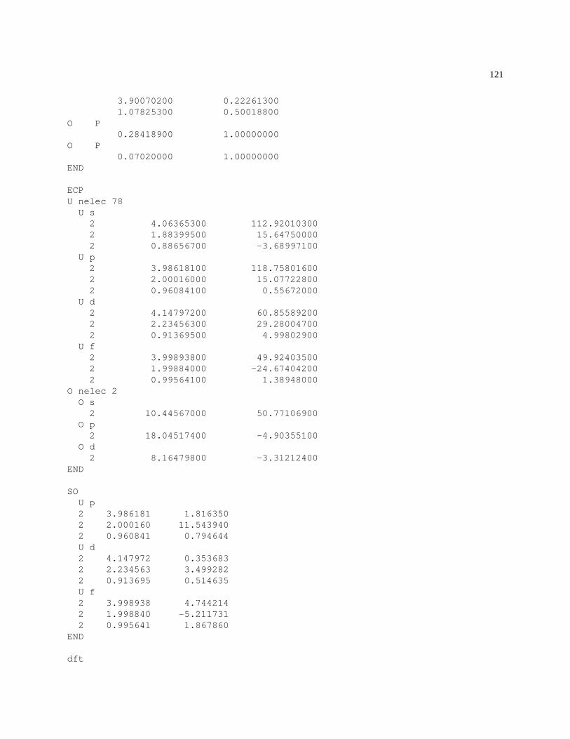
121
3.90070200 0.222613001.07825300 0.50018800
O P0.28418900 1.00000000
O P0.07020000 1.00000000
END
ECPU nelec 78
U s2 4.06365300 112.920103002 1.88399500 15.647500002 0.88656700 -3.68997100
U p2 3.98618100 118.758016002 2.00016000 15.077228002 0.96084100 0.55672000
U d2 4.14797200 60.855892002 2.23456300 29.280047002 0.91369500 4.99802900
U f2 3.99893800 49.924035002 1.99884000 -24.674042002 0.99564100 1.38948000
O nelec 2O s
2 10.44567000 50.77106900O p
2 18.04517400 -4.90355100O d
2 8.16479800 -3.31212400END
SOU p2 3.986181 1.8163502 2.000160 11.5439402 0.960841 0.794644U d2 4.147972 0.3536832 2.234563 3.4992822 0.913695 0.514635U f2 3.998938 4.7442142 1.998840 -5.2117312 0.995641 1.867860
END
dft

122 CHAPTER 12. SPIN-ORBIT DFT (SODFT)
mult 1xc hfexchodftgrid fineconvergence energy 1.000000E-06convergence density 1.000000E-05convergence gradient 1E-05iterations 100mulliken
end
task sodft
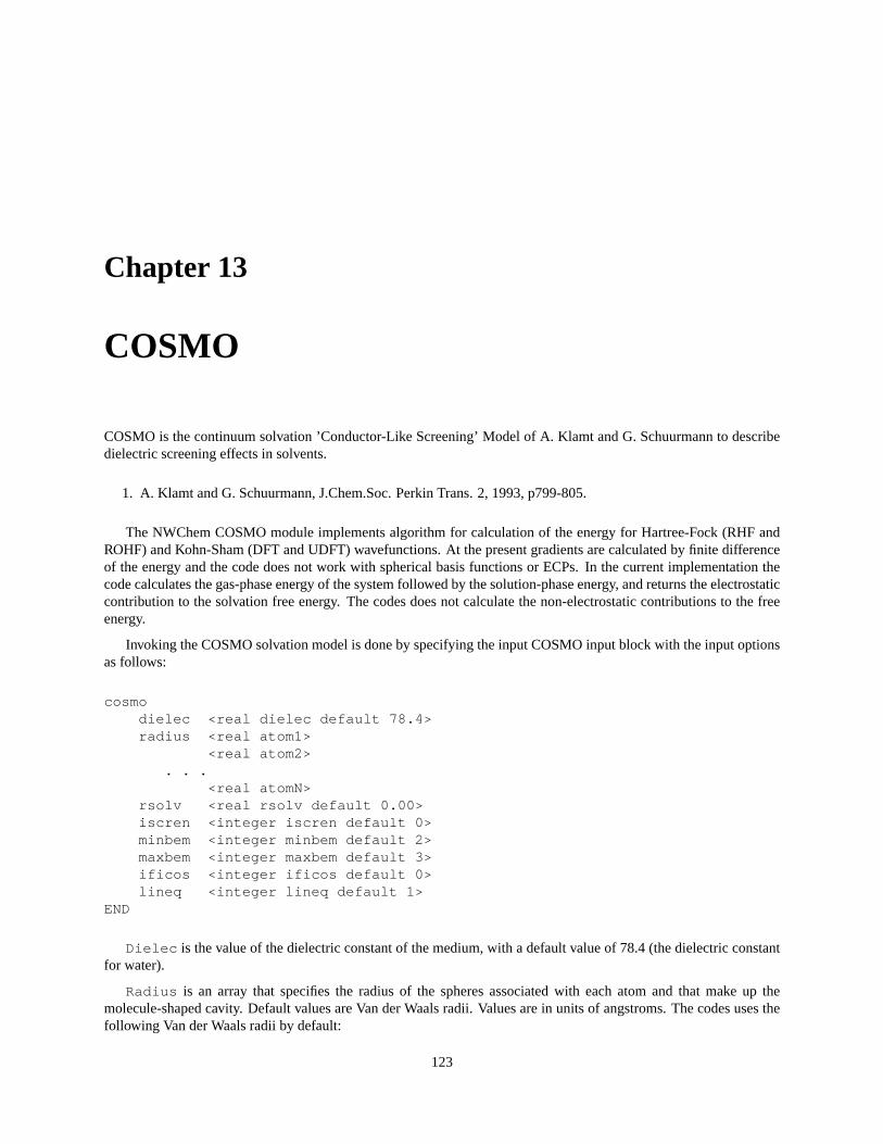
Chapter 13
COSMO
COSMO is the continuum solvation ’Conductor-Like Screening’ Model of A. Klamt and G. Schuurmann to describedielectric screening effects in solvents.
1. A. Klamt and G. Schuurmann, J.Chem.Soc. Perkin Trans. 2, 1993, p799-805.
The NWChem COSMO module implements algorithm for calculation of the energy for Hartree-Fock (RHF andROHF) and Kohn-Sham (DFT and UDFT) wavefunctions. At the present gradients are calculated by finite differenceof the energy and the code does not work with spherical basis functions or ECPs. In the current implementation thecode calculates the gas-phase energy of the system followed by the solution-phase energy, and returns the electrostaticcontribution to the solvation free energy. The codes does not calculate the non-electrostatic contributions to the freeenergy.
Invoking the COSMO solvation model is done by specifying the input COSMO input block with the input optionsas follows:
cosmodielec <real dielec default 78.4>radius <real atom1>
<real atom2>. . .
<real atomN>rsolv <real rsolv default 0.00>iscren <integer iscren default 0>minbem <integer minbem default 2>maxbem <integer maxbem default 3>ificos <integer ificos default 0>lineq <integer lineq default 1>
END
Dielec is the value of the dielectric constant of the medium, with a default value of 78.4 (the dielectric constantfor water).
Radius is an array that specifies the radius of the spheres associated with each atom and that make up themolecule-shaped cavity. Default values are Van der Waals radii. Values are in units of angstroms. The codes uses thefollowing Van der Waals radii by default:
123
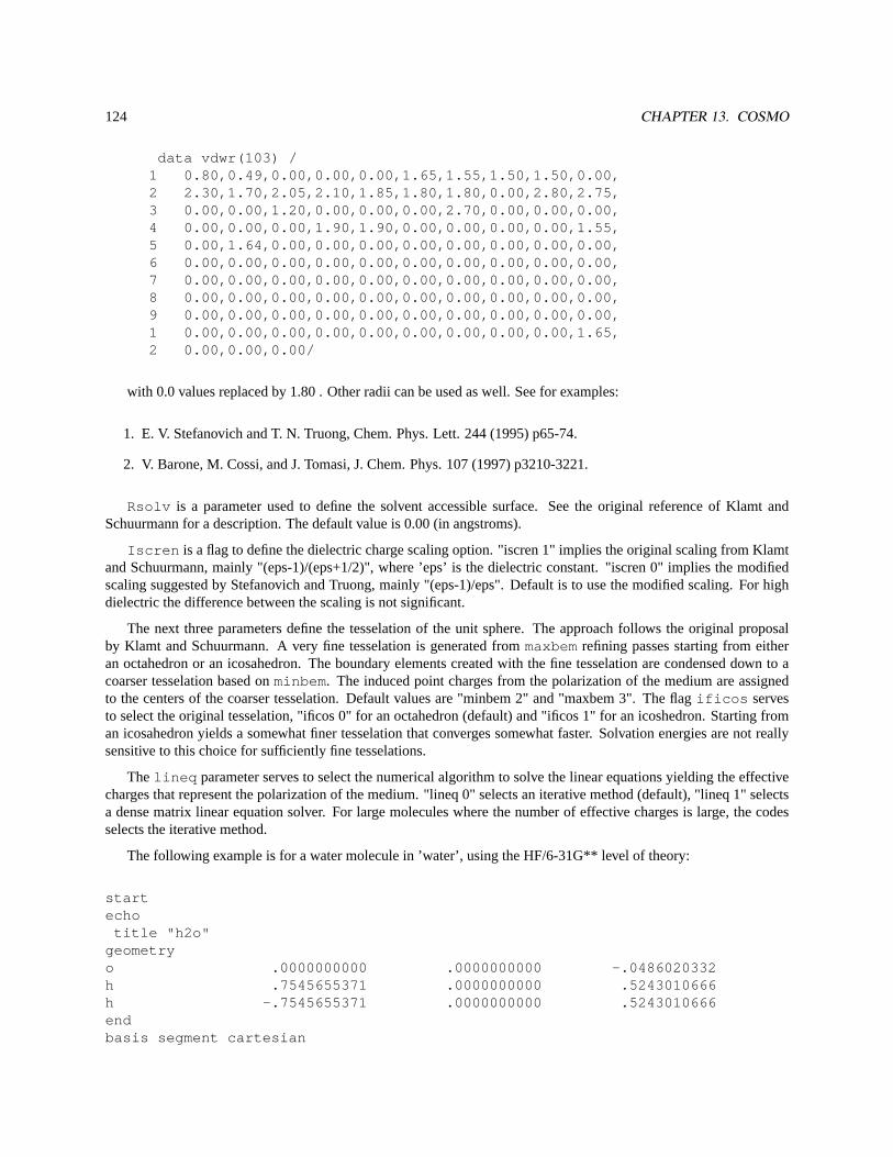
124 CHAPTER 13. COSMO
data vdwr(103) /1 0.80,0.49,0.00,0.00,0.00,1.65,1.55,1.50,1.50,0.00,2 2.30,1.70,2.05,2.10,1.85,1.80,1.80,0.00,2.80,2.75,3 0.00,0.00,1.20,0.00,0.00,0.00,2.70,0.00,0.00,0.00,4 0.00,0.00,0.00,1.90,1.90,0.00,0.00,0.00,0.00,1.55,5 0.00,1.64,0.00,0.00,0.00,0.00,0.00,0.00,0.00,0.00,6 0.00,0.00,0.00,0.00,0.00,0.00,0.00,0.00,0.00,0.00,7 0.00,0.00,0.00,0.00,0.00,0.00,0.00,0.00,0.00,0.00,8 0.00,0.00,0.00,0.00,0.00,0.00,0.00,0.00,0.00,0.00,9 0.00,0.00,0.00,0.00,0.00,0.00,0.00,0.00,0.00,0.00,1 0.00,0.00,0.00,0.00,0.00,0.00,0.00,0.00,0.00,1.65,2 0.00,0.00,0.00/
with 0.0 values replaced by 1.80 . Other radii can be used as well. See for examples:
1. E. V. Stefanovich and T. N. Truong, Chem. Phys. Lett. 244 (1995) p65-74.
2. V. Barone, M. Cossi, and J. Tomasi, J. Chem. Phys. 107 (1997) p3210-3221.
Rsolv is a parameter used to define the solvent accessible surface. See the original reference of Klamt andSchuurmann for a description. The default value is 0.00 (in angstroms).
Iscren is a flag to define the dielectric charge scaling option. "iscren 1" implies the original scaling from Klamtand Schuurmann, mainly "(eps-1)/(eps+1/2)", where ’eps’ is the dielectric constant. "iscren 0" implies the modifiedscaling suggested by Stefanovich and Truong, mainly "(eps-1)/eps". Default is to use the modified scaling. For highdielectric the difference between the scaling is not significant.
The next three parameters define the tesselation of the unit sphere. The approach follows the original proposalby Klamt and Schuurmann. A very fine tesselation is generated frommaxbemrefining passes starting from eitheran octahedron or an icosahedron. The boundary elements created with the fine tesselation are condensed down to acoarser tesselation based onminbem. The induced point charges from the polarization of the medium are assignedto the centers of the coarser tesselation. Default values are "minbem 2" and "maxbem 3". The flagificos servesto select the original tesselation, "ificos 0" for an octahedron (default) and "ificos 1" for an icoshedron. Starting froman icosahedron yields a somewhat finer tesselation that converges somewhat faster. Solvation energies are not reallysensitive to this choice for sufficiently fine tesselations.
The lineq parameter serves to select the numerical algorithm to solve the linear equations yielding the effectivecharges that represent the polarization of the medium. "lineq 0" selects an iterative method (default), "lineq 1" selectsa dense matrix linear equation solver. For large molecules where the number of effective charges is large, the codesselects the iterative method.
The following example is for a water molecule in ’water’, using the HF/6-31G** level of theory:
startecho
title "h2o"geometryo .0000000000 .0000000000 -.0486020332h .7545655371 .0000000000 .5243010666h -.7545655371 .0000000000 .5243010666endbasis segment cartesian
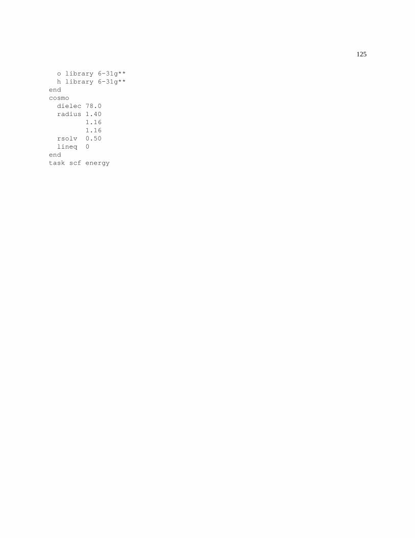
125
o library 6-31g**h library 6-31g**
endcosmo
dielec 78.0radius 1.40
1.161.16
rsolv 0.50lineq 0
endtask scf energy

126 CHAPTER 13. COSMO
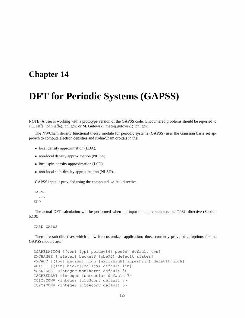
Chapter 14
DFT for Periodic Systems (GAPSS)
NOTE: A user is working with a prototype version of the GAPSS code. Encountered problems should be reported toJ.E. Jaffe, [email protected], or M. Gutowski, [email protected].
The NWChem density functional theory module for periodic systems (GAPSS) uses the Gaussian basis set ap-proach to compute electron densities and Kohn-Sham orbitals in the:
• local density approximation (LDA),
• non-local density approximation (NLDA),
• local spin-density approximation (LSD),
• non-local spin-density approximation (NLSD).
GAPSS input is provided using the compoundGAPSSdirective
GAPSS...
END
The actual DFT calculation will be performed when the input module encounters theTASK directive (Section5.10).
TASK GAPSS
There are sub-directives which allow for customized application; those currently provided as options for theGAPSS module are:
CORRELATION [(vwn||lyp||perdew86||pbe96) default vwn]EXCHANGE [(slater||becke88||pbe96) default slater]VXCACC [(low||medium||high||extrahigh||superhigh) default high]WEIGHT [(lin||becke||delley) default lin]MONKHORST <integer monkhorst default 3>ISCREENLAT <integer iscreenlat default 7>IC1C3CONV <integer ic1c3conv default 7>IC2C4CONV <integer ic2c4conv default 6>
127
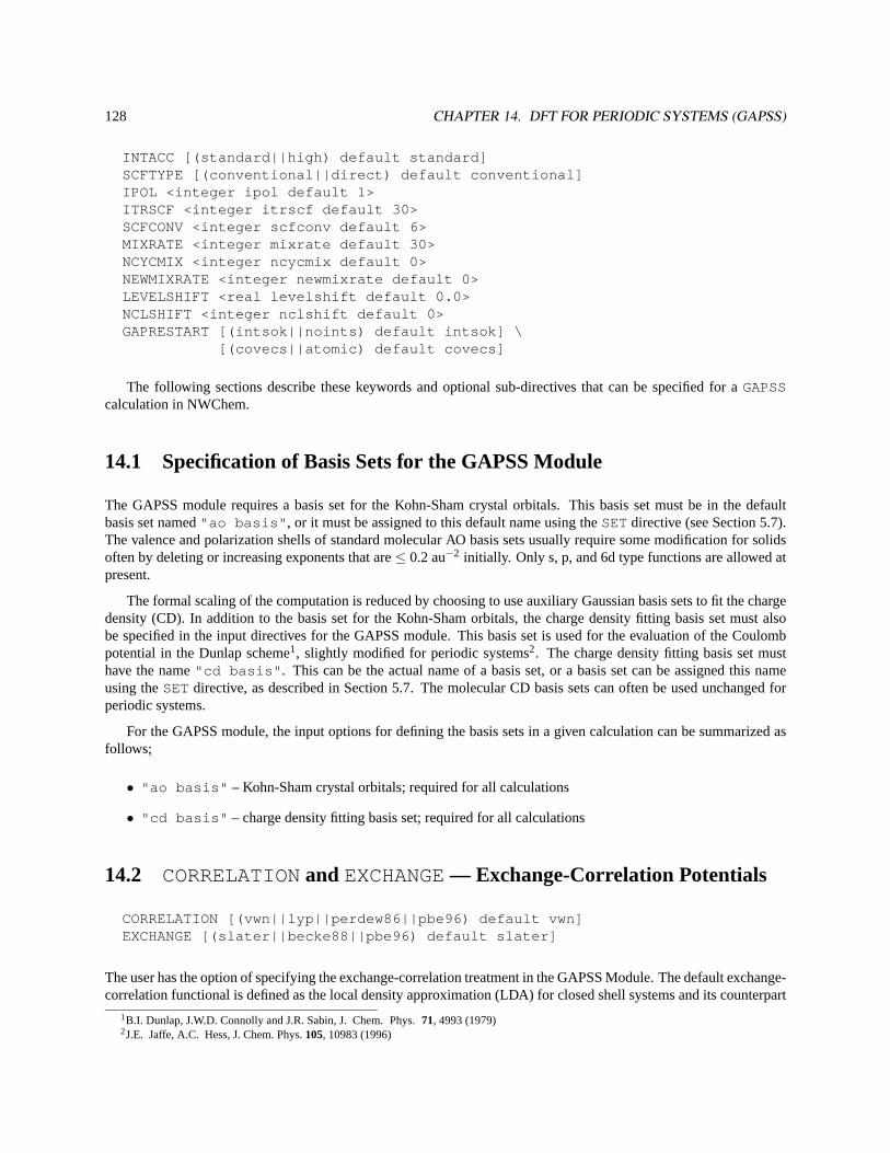
128 CHAPTER 14. DFT FOR PERIODIC SYSTEMS (GAPSS)
INTACC [(standard||high) default standard]SCFTYPE [(conventional||direct) default conventional]IPOL <integer ipol default 1>ITRSCF <integer itrscf default 30>SCFCONV <integer scfconv default 6>MIXRATE <integer mixrate default 30>NCYCMIX <integer ncycmix default 0>NEWMIXRATE <integer newmixrate default 0>LEVELSHIFT <real levelshift default 0.0>NCLSHIFT <integer nclshift default 0>GAPRESTART [(intsok||noints) default intsok] \
[(covecs||atomic) default covecs]
The following sections describe these keywords and optional sub-directives that can be specified for aGAPSScalculation in NWChem.
14.1 Specification of Basis Sets for the GAPSS Module
The GAPSS module requires a basis set for the Kohn-Sham crystal orbitals. This basis set must be in the defaultbasis set named"ao basis" , or it must be assigned to this default name using theSETdirective (see Section 5.7).The valence and polarization shells of standard molecular AO basis sets usually require some modification for solidsoften by deleting or increasing exponents that are≤ 0.2 au−2 initially. Only s, p, and 6d type functions are allowed atpresent.
The formal scaling of the computation is reduced by choosing to use auxiliary Gaussian basis sets to fit the chargedensity (CD). In addition to the basis set for the Kohn-Sham orbitals, the charge density fitting basis set must alsobe specified in the input directives for the GAPSS module. This basis set is used for the evaluation of the Coulombpotential in the Dunlap scheme1, slightly modified for periodic systems2. The charge density fitting basis set musthave the name"cd basis" . This can be the actual name of a basis set, or a basis set can be assigned this nameusing theSET directive, as described in Section 5.7. The molecular CD basis sets can often be used unchanged forperiodic systems.
For the GAPSS module, the input options for defining the basis sets in a given calculation can be summarized asfollows;
• "ao basis" – Kohn-Sham crystal orbitals; required for all calculations
• "cd basis" – charge density fitting basis set; required for all calculations
14.2 CORRELATIONand EXCHANGE— Exchange-Correlation Potentials
CORRELATION [(vwn||lyp||perdew86||pbe96) default vwn]EXCHANGE [(slater||becke88||pbe96) default slater]
The user has the option of specifying the exchange-correlation treatment in the GAPSS Module. The default exchange-correlation functional is defined as the local density approximation (LDA) for closed shell systems and its counterpart
1B.I. Dunlap, J.W.D. Connolly and J.R. Sabin, J. Chem. Phys.71, 4993 (1979)2J.E. Jaffe, A.C. Hess, J. Chem. Phys.105, 10983 (1996)
14.2. CORRELATIONAND EXCHANGE— EXCHANGE-CORRELATION POTENTIALS 129
the local spin-density (LSD) approximation for open shell systems. Within this approximation the exchange functionalis the Slaterρ1/3 functional (from J.C. Slater,Quantum Theory of Molecules and Solids, Vol. 4: The Self-ConsistentField for Molecules and Solids (McGraw-Hill, New York, 1974)), and the correlation functional is the Vosko-Wilk-Nusair (VWN) functional (functional V) (S.J. Vosko, L. Wilk and M. Nusair, Can. J. Phys.58, 1200 (1980)). Theparameters used in this formula are obtained by fitting to the Ceperley and Alder3 Quantum Monte-Carlo solution ofthehomogeneous electron gas.
These defaults can be invoked explicitly by specifying the following keywords within the GAPSS module inputdirective,
CORRELATION vwnEXCHANGE slater
Several alternative exchange and correlation functionals are available to the user. The following sections describethese options.
14.2.1 Optional Functionals
There are two exchange functionals in addition to the default Slater exchange functional. These are the Becke gradient-corrected functional (see A.D. Becke, J. Chem. Phys. 88, 3098 (1988)), and the Perdew, Burke, Ernzerhof generalizedgradient approximation to the exchange-correlation functional (see J.P. Perdew, K. Burke, M. Ernzerhof, Phys. Rev.Lett. 77, 3865 (1996)).
The Becke gradient-corrected functional is invoked by specifying the input line
EXCHANGE becke88
The Perdew, Burke, Ernzerhof exchange functional is invoked by specifying the input line
EXCHANGE pbe96
There are three correlation functionals in addition to the default vwn correlation functional. These are the LYPgradient-corrected functional (C. Lee, W. Yang and R. G. Parr, Phys. Rev. B37, 785 (1988)), Perdew86 gradient-corrected functional (J. P. Perdew, Phys. Rev. B33, 8822 (1986)), and the Perdew, Burke, Ernzerhof generalizedgradient approximation to the exchange-correlation functional (J.P. Perdew, K. Burke, M. Ernzerhof, Phys. Rev.Lett. 77, 3865 (1996)).
The LYP gradient-corrected functional is invoked by specifying the input line
CORRELATION lyp
The Perdew86 gradient-corrected functional is invoked by specifying the input line
CORRELATION perdew86
The Perdew, Burke, Ernzerhof correlation functional is invoked by specifying the input line
CORRELATION pbe96
3D.M. Ceperley and B.J. Alder, Phys. Rev. Lett.45, 566 (1980).
130 CHAPTER 14. DFT FOR PERIODIC SYSTEMS (GAPSS)
14.3 Numerical Integration
VXCACC [(low||medium||high||extrahigh||superhigh) default high]
A numerical integration is necessary for the evaluation of the exchange-correlation contribution to the total energyand the Fock matrices. The user can specify the level of accuracy with the keywords; low, medium, high, extrahigh,superhigh. The default is high which corresponds to accuracy of ca. 1e-4 for the XC potential and energy. Each levelof higher accuracy improves the accuracy of integration by a factor≈ 10 and increases the cost by a factor of≈ 3.
WEIGHT [(lin||becke||delley) default lin]
The three-dimensional integration is reduced to a sum of one-center, atomic-like integrations using either the Lin andHess scheme (Z. Lin, J.E. Jaffe, A.C. Hess, J. Phys. Chem. A 103, 2117 (1999))
WEIGHT lin
or the Becke scheme (A.D. Becke, J. Chem. Phys. 88, 2547 (1988))
WEIGHT becke
or the Delley scheme (B. Delley, J. Chem. Phys. 92, 508 (1990))
WEIGHT delley
14.4 Summations and Integrations for a Periodic System
MONKHORST <integer monkhorst default 3>ISCREENLAT <integer iscreenlat default 7>IC1C3CONV <integer ic1c3conv default 7>IC2C4CONV <integer ic2c4conv default 6>INTACC [(standard||high) default standard]
The wave vectors in the first Brillouin zone are sampled following the Monkhorst-Pack scheme4 MONKHORST= 5 isrecommended for systems with 1-2 atoms per primitive unit cell, smaller values may be used for larger cells. Metals atpresent requireMONKHORST≥ 10. The convergence of the C1-C3 and C2-C4 series is controlled by the IC1C3CONVand IC2C4CONV directives, respectively, see J.E. Jaffe, A.C. Hess, J. Chem. Phys.105, 10983 (1996), and theaccuracy of H(k) and S(k) with respect to the summation over unit cells is controlled by the ISCREENLAT directive.ISCREENLAT= 7 produces errors≈ 10−6 Eh, with each higher level reducing this error by ca. 1 order of magnitudeat little extra cost.IC1C3CONV= ISCREENLATandIC2C4CONV= ISCREENLAT- 1 are recommended. Finally,the accuracy of two-electron three-center integrals is controlled by the directive INTACC.
14.5 SCF Iterative Procedure
SCFTYPE [(conventional||direct) default conventional]4H.J. Monkhorst and J.D. Pack, Phys. Rev. B.13, 5188 (1976).
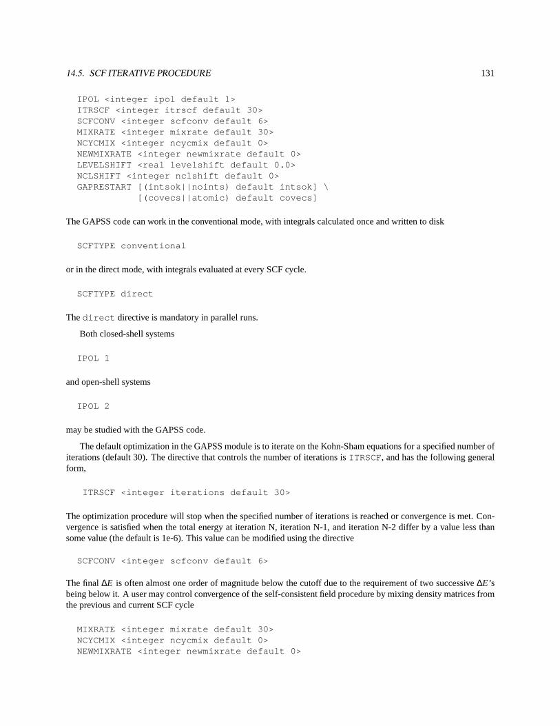
14.5. SCF ITERATIVE PROCEDURE 131
IPOL <integer ipol default 1>ITRSCF <integer itrscf default 30>SCFCONV <integer scfconv default 6>MIXRATE <integer mixrate default 30>NCYCMIX <integer ncycmix default 0>NEWMIXRATE <integer newmixrate default 0>LEVELSHIFT <real levelshift default 0.0>NCLSHIFT <integer nclshift default 0>GAPRESTART [(intsok||noints) default intsok] \
[(covecs||atomic) default covecs]
The GAPSS code can work in the conventional mode, with integrals calculated once and written to disk
SCFTYPE conventional
or in the direct mode, with integrals evaluated at every SCF cycle.
SCFTYPE direct
Thedirect directive is mandatory in parallel runs.
Both closed-shell systems
IPOL 1
and open-shell systems
IPOL 2
may be studied with the GAPSS code.
The default optimization in the GAPSS module is to iterate on the Kohn-Sham equations for a specified number ofiterations (default 30). The directive that controls the number of iterations isITRSCF, and has the following generalform,
ITRSCF <integer iterations default 30>
The optimization procedure will stop when the specified number of iterations is reached or convergence is met. Con-vergence is satisfied when the total energy at iteration N, iteration N-1, and iteration N-2 differ by a value less thansome value (the default is 1e-6). This value can be modified using the directive
SCFCONV <integer scfconv default 6>
The final∆E is often almost one order of magnitude below the cutoff due to the requirement of two successive∆E’sbeing below it. A user may control convergence of the self-consistent field procedure by mixing density matrices fromthe previous and current SCF cycle
MIXRATE <integer mixrate default 30>NCYCMIX <integer ncycmix default 0>NEWMIXRATE <integer newmixrate default 0>
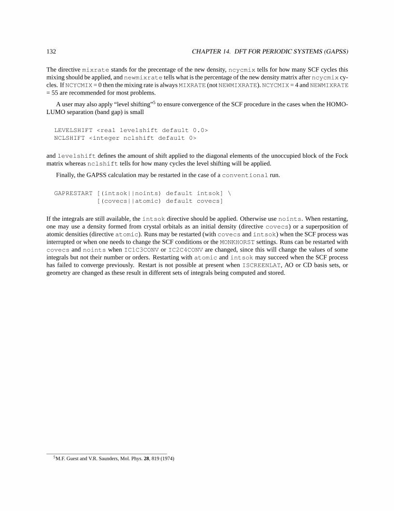
132 CHAPTER 14. DFT FOR PERIODIC SYSTEMS (GAPSS)
The directivemixrate stands for the precentage of the new density,ncycmix tells for how many SCF cycles thismixing should be applied, andnewmixrate tells what is the percentage of the new density matrix afterncycmix cy-cles. IfNCYCMIX= 0 then the mixing rate is alwaysMIXRATE(notNEWMIXRATE). NCYCMIX= 4 andNEWMIXRATE= 55 are recommended for most problems.
A user may also apply “level shifting”5 to ensure convergence of the SCF procedure in the cases when the HOMO-LUMO separation (band gap) is small
LEVELSHIFT <real levelshift default 0.0>NCLSHIFT <integer nclshift default 0>
andlevelshift defines the amount of shift applied to the diagonal elements of the unoccupied block of the Fockmatrix whereasnclshift tells for how many cycles the level shifting will be applied.
Finally, the GAPSS calculation may be restarted in the case of aconventional run.
GAPRESTART [(intsok||noints) default intsok] \[(covecs||atomic) default covecs]
If the integrals are still available, theintsok directive should be applied. Otherwise usenoints . When restarting,one may use a density formed from crystal orbitals as an initial density (directivecovecs ) or a superposition ofatomic densities (directiveatomic ). Runs may be restarted (withcovecs andintsok ) when the SCF process wasinterrupted or when one needs to change the SCF conditions or theMONKHORSTsettings. Runs can be restarted withcovecs andnoints when IC1C3CONVor IC2C4CONVare changed, since this will change the values of someintegrals but not their number or orders. Restarting withatomic andintsok may succeed when the SCF processhas failed to converge previously. Restart is not possible at present whenISCREENLAT, AO or CD basis sets, orgeometry are changed as these result in different sets of integrals being computed and stored.
5M.F. Guest and V.R. Saunders, Mol. Phys.28, 819 (1974)
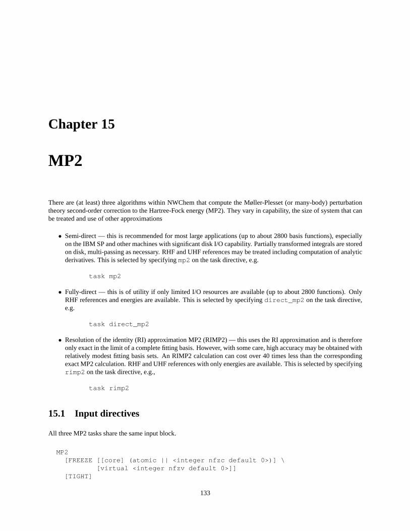
Chapter 15
MP2
There are (at least) three algorithms within NWChem that compute the Møller-Plesset (or many-body) perturbationtheory second-order correction to the Hartree-Fock energy (MP2). They vary in capability, the size of system that canbe treated and use of other approximations
• Semi-direct — this is recommended for most large applications (up to about 2800 basis functions), especiallyon the IBM SP and other machines with significant disk I/O capability. Partially transformed integrals are storedon disk, multi-passing as necessary. RHF and UHF references may be treated including computation of analyticderivatives. This is selected by specifyingmp2on the task directive, e.g.
task mp2
• Fully-direct — this is of utility if only limited I/O resources are available (up to about 2800 functions). OnlyRHF references and energies are available. This is selected by specifyingdirect_mp2 on the task directive,e.g.
task direct_mp2
• Resolution of the identity (RI) approximation MP2 (RIMP2) — this uses the RI approximation and is thereforeonly exact in the limit of a complete fitting basis. However, with some care, high accuracy may be obtained withrelatively modest fitting basis sets. An RIMP2 calculation can cost over 40 times less than the correspondingexact MP2 calculation. RHF and UHF references with only energies are available. This is selected by specifyingrimp2 on the task directive, e.g.,
task rimp2
15.1 Input directives
All three MP2 tasks share the same input block.
MP2[FREEZE [[core] (atomic || <integer nfzc default 0>)] \
[virtual <integer nfzv default 0>]][TIGHT]
133
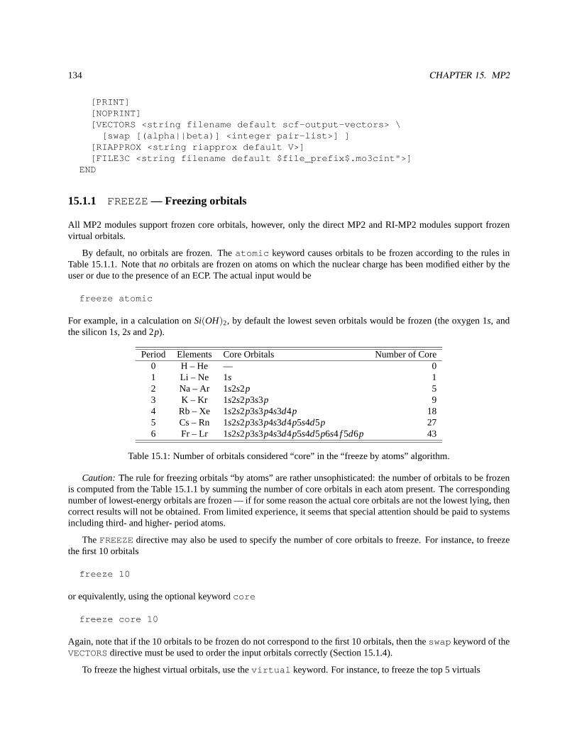
134 CHAPTER 15. MP2
[PRINT][NOPRINT][VECTORS <string filename default scf-output-vectors> \
[swap [(alpha||beta)] <integer pair-list>] ][RIAPPROX <string riapprox default V>][FILE3C <string filename default $file_prefix$.mo3cint">]
END
15.1.1 FREEZE— Freezing orbitals
All MP2 modules support frozen core orbitals, however, only the direct MP2 and RI-MP2 modules support frozenvirtual orbitals.
By default, no orbitals are frozen. Theatomic keyword causes orbitals to be frozen according to the rules inTable 15.1.1. Note thatno orbitals are frozen on atoms on which the nuclear charge has been modified either by theuser or due to the presence of an ECP. The actual input would be
freeze atomic
For example, in a calculation onSi(OH)2, by default the lowest seven orbitals would be frozen (the oxygen 1s, andthe silicon 1s, 2s and 2p).
Period Elements Core Orbitals Number of Core0 H – He — 01 Li – Ne 1s 12 Na – Ar 1s2s2p 53 K – Kr 1s2s2p3s3p 94 Rb – Xe 1s2s2p3s3p4s3d4p 185 Cs – Rn 1s2s2p3s3p4s3d4p5s4d5p 276 Fr – Lr 1s2s2p3s3p4s3d4p5s4d5p6s4 f 5d6p 43
Table 15.1: Number of orbitals considered “core” in the “freeze by atoms” algorithm.
Caution: The rule for freezing orbitals “by atoms” are rather unsophisticated: the number of orbitals to be frozenis computed from the Table 15.1.1 by summing the number of core orbitals in each atom present. The correspondingnumber of lowest-energy orbitals are frozen — if for some reason the actual core orbitals are not the lowest lying, thencorrect results will not be obtained. From limited experience, it seems that special attention should be paid to systemsincluding third- and higher- period atoms.
TheFREEZEdirective may also be used to specify the number of core orbitals to freeze. For instance, to freezethe first 10 orbitals
freeze 10
or equivalently, using the optional keywordcore
freeze core 10
Again, note that if the 10 orbitals to be frozen do not correspond to the first 10 orbitals, then theswap keyword of theVECTORSdirective must be used to order the input orbitals correctly (Section 15.1.4).
To freeze the highest virtual orbitals, use thevirtual keyword. For instance, to freeze the top 5 virtuals
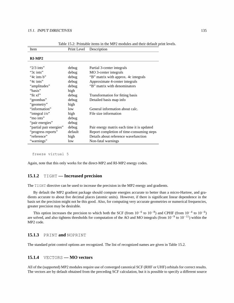
15.1. INPUT DIRECTIVES 135
Table 15.2: Printable items in the MP2 modules and their default print levels.
Item Print Level Description
RI-MP2
“2/3 ints” debug Partial 3-center integrals“3c ints” debug MO 3-center integrals“4c ints b” debug “B” matrix with approx. 4c integrals“4c ints” debug Approximate 4-center integrals“amplitudes” debug “B” matrix with denominators“basis” high“fit xf” debug Transformation for fitting basis“geombas” debug Detailed basis map info“geometry” high“information” low General information about calc.“integral i/o” high File size information“mo ints” debug“pair energies” debug“partial pair energies” debug Pair energy matrix each time it is updated“progress reports” default Report completion of time-consuming steps“reference” high Details about reference wavefunction“warnings” low Non-fatal warnings
freeze virtual 5
Again, note that this only works for the direct-MP2 and RI-MP2 energy codes.
15.1.2 TIGHT — Increased precision
TheTIGHT directive can be used to increase the precision in the MP2 energy and gradients.
By default the MP2 gradient package should compute energies accurate to better than a micro-Hartree, and gra-dients accurate to about five decimal places (atomic units). However, if there is significant linear dependence in thebasis set the precision might not be this good. Also, for computing very accurate geometries or numerical frequencies,greater precision may be desirable.
This option increases the precision to which both the SCF (from 10−6 to 10−8) and CPHF (from 10−4 to 10−6)are solved, and also tightens thresholds for computation of the AO and MO integrals (from 10−9 to 10−11) within theMP2 code.
15.1.3 PRINT and NOPRINT
The standard print control options are recognized. The list of recognized names are given in Table 15.2.
15.1.4 VECTORS— MO vectors
All of the (supported) MP2 modules require use of converged canonical SCF (RHF or UHF) orbitals for correct results.The vectors are by default obtained from the preceding SCF calculation, but it is possible to specify a different source
136 CHAPTER 15. MP2
using theVECTORSdirective. For instance, to obtain vectors from the file/tmp/h2o.movecs , use the directive
vectors /tmp/h2o.movecs
As noted above (Section 15.1.1) if the SCF orbitals are not in the correct order, it is necessary to permute theinput orbitals using theswap keyword of theVECTORSdirective. For instance, if it is desired to freeze a total sixorbitals corresponding to the SCF orbitals 1–5, and 7, it is necessary to swap orbital 7 into the 6th position. This isaccomplished by
vectors swap 6 7
The swap capability is examined in more detail in Section 10.5.
15.1.5 RI-MP2 fitting basis
The RI-MP2 method requires a fitting basis, which must be specified with the name"ri-mp2 basis" (see Section7). For instance,
basis "ri-mp2 basis"O s; 10000.0 1O s; 1000.0 1O s; 100.0 1...
end
Alternatively, using a standard capability of basis sets (Section 7) another named basis may be associated with thefitting basis. For instance, the following input specifies a basis with the name"small fitting basis" and thendefines this to be the"ri-mp2 basis" .
basis "small fitting basis"H s; 10 1H s; 3 1H s; 1 1H s; 0.1 1H s; 0.01 1
end
set "ri-mp2 basis" "small fitting basis"
15.1.6 FILE3C — RI-MP2 3-center integral filename
The default name for the file used to store the transformed 3-center integrals is"$file_prefix$.mo3cint"in the scratch directory. This may be overridden using the FILE3C directive. For instance, to specify the file/scratch/h2o.3c , use this directive
file3c /scratch/h2o.3c
15.1. INPUT DIRECTIVES 137
15.1.7 RIAPPROX— RI-MP2 Approximation
The type of RI approximation used in the RI-MP2 calculation is controlled by means of the RIAPPROX directive.The two possible values areV andSVS(case sensitive), which correspond to the approximations with the same namesdescribed in O. Vahtras, J Almlöf, and M. W. Feyereisen,Chem. Phys. Lett.213, 514–518 (1993). The default isV.
15.1.8 Advanced options for RI-MP2
These options, which functioned at the time of writing, are not currently supported.
Control of linear dependence
Construction of the RI fit requires the inversion of a matrix of fitting basis integrals which is carried out via diago-nalization. If the fitting basis includes near linear dependencies, there will be small eigenvalues which can ultimatelylead to non-physical RI-MP2 correlation energies. Eigenvectors of the fitting matrix are discarded if the correspond-ing eigenvalue is less than$mineval$ which defaults to 10−8. This parameter may be changed by setting the aparameter in the database. For instance, to set it to 10−10
set "mp2:fit min eval" 1e-10
Reference Spin Mapping for RI-MP2 Calculations
The user has the option of specifying that the RI-MP2 calculations are to be done with variations of the SCF referencewavefunction. This is accomplished with aSETdirective of the form,
set "mp2:reference spin mapping" <integer array default 0>
Each element specified forarray is the SCF spin case to be used for the corresponding spin case of the correlatedcalculation. The number of elements set determines the overall type of correlated calculation to be performed. Thedefault is to use the unadulterated SCF reference wavefunction.
For example, to perform a spin-unrestricted calculation (two elements) using the alpha spin orbitals (spin case 1)from the reference for both of the correlated reference spin cases, theSETdirective would be as follows,
set "mp2:reference spin mapping" 1 1
The SCF calculation to produce the reference wavefunction could be either RHF or UHF in this case.
TheSETdirective for a similar case, but this time using the beta-spin SCF orbitals for both correlated spin cases,is as follows,
set "mp2:reference spin mapping" 2 2
The SCF reference calculation must be UHF in this case.
TheSETdirective for a spin-restricted calculation (one element) from the beta-spin SCF orbitals using this optionis as follows,
set "mp2:reference spin mapping" 2
138 CHAPTER 15. MP2
TheSETdirective for a spin-unrestricted calculation with the spins flipped from the original SCF reference wave-function is as follows,
set "mp2:reference spin mapping" 2 1
Batch Sizes for the RI-MP2 Calculation
The user can control the size of each batch in the transformation and energy evaluation in the MP2 calculation, andconsequently the memory requirements and number of passes required. This is done using twoSETdirectives of thefollowing form,
set "mp2:transformation batch size" <integer size default -1>set "mp2:energy batch size" <integer isize jsize default -1 -1>
The default is for the code to determine the batch size based on the available memory. Should there be problemswith the program-determined batch sizes, these variables allow the user to override them. The program will alwaysuse the smaller of the user’s value of these entries and the internally computed batch size.
The transformation batch size computed in the code is the number of occupied orbitals in the(occ vir| f it ) three-center integrals to be produced at a time. If this entry is less than the number of occupied orbitals in the system, thetransformation will require multiple passes through the two-electron integrals. The memory requirements of this stagearetwoglobal arrays of dimension< batchsize>×vir× f it with the “fit” dimension distributed across all processors(on shell-block boundaries). The compromise here is memory space versus multiple integral evaluations.
The energy evaluation batch sizes are computed in the code from the number of occupied orbitals in the two sets ofthree-center integrals to be multiplied together to produce a matrix of approximate four-center integrals. Two blocksof integrals of dimension(< batchisize>×vir) and(< batch jsize>×vir) by fit are read in from disk and multipliedtogether to produce< batchisize>< batch jsize> vir2 approximate integrals. The compromise here is performanceof the distributed matrix multiplication (which requires large matrices) versus memory space.
Energy Memory Allocation Mode: RI-MP2 Calculation
The user must choose a strategy for the memory allocation in the energy evaluation phase of the RI-MP2 calculation,either by minimizing the amount of I/O, or minimizing the amount of computation. This can be accomplished using aSETdirective of the form,
set "mp2:energy mem minimize" <string mem_opt default I>
A value of I entered for the stringmem_opt means that a strategy to minimize I/O will be employed. A value ofC tells the code to use a strategy that minimizes computation.
When the option to minimize I/O is selected, the block sizes are made as large as possible so that the total numberof passes through the integral files is as small as possible. When the option to minimize computation is selected, theblocks are chosen as close to square as possible so that permutational symmetry in the energy evaluation can be usedmost effectively.
Local Memory Usage in Three-Center Transformation
For most applications, the code will be able to size the blocks without help from the user. Therefore, it is unlikelythat users will have any reason to specify values for these entries except when doing very particular performancemeasurements.
15.2. ONE-ELECTRON PROPERTIES AND NATURAL ORBITALS 139
The size ofxf3ci:AO 1 batch size is the most important of the three, in terms of the effect on performance.
Local memory usage in the first two steps of the transformation is controlled in the RI-MP2 calculation using thefollowing SETdirectives,
set "xf3ci:AO 1 batch size" <integer max>set "xf3ci:AO 2 batch size" <integer max>set "xf3ci:fit batch size" <integer max>
The size of the local arrays determines the sizes of the two matrix multiplications. These entries set limits on thesize of blocks to be used in each index. The listing above is in order of importance of the parameters to performance,with xf3ci:AO 1 batch size being most important.
Note that these entries are only upper bounds and that the program will size the blocks according to what itdetermines as the best usage of the available local memory. The absolute maximum for a block size is the number offunctions in the AO basis, or the number of fitting basis functions on a node. The absolute minimum value for blocksize is the size of the largest shell in the appropriate basis. Batch size entries specified formax that are larger thanthese limits are automatically reset to an appropriate value.
15.2 One-electron properties and natural orbitals
If an MP2 energy gradient is computed, all contributions are available to form the MP2 linear-response density. Thisis the density that when contracted with any spin-free, one-electron operator yields the associated property defined asthe derivative of the energy. Thus, the reported MP2 dipole moment is the derivative of the energy w.r.t. an externalmagnetic field and isnot the expectation value of the operator over the wavefunction. Only dipole moments are printedby the MP2 gradient code, but natural orbitals are produced and stored in the permanent directory with a file extensionof ".mp2nos" . These may be fed into the property package (see Section 24) to compute more general properties.Note that the MP2 linear response density matrix is not necessarily positive definite so it is not unusual to see a fewsmall negative natural orbital occupation numbers.

140 CHAPTER 15. MP2
Chapter 16
Multiconfiguration SCF
The NWChem multiconfiguration SCF (MCSCF) module can currently perform complete active space SCF (CASSCF)calculations with at most 20 active orbitals and about 500 basis functions. It is planned to extend it to handle 1000+basis functions.
MCSCFSTATE <string state>ACTIVE <integer nactive>ACTELEC <integer nactelec>MULTIPLICITY <integer multiplicity>[SYMMETRY <integer symmetry default 1>][VECTORS [[input] <string input_file default $file_prefix$.movecs>]
[swap <integer vec1 vec2> ...] \[output <string output_file default input_file>] \[lock]
[HESSIAN (exact||onel)][MAXITER <integer maxiter default 20>][THRESH <real thresh default 1.0e-4>][TOL2E <real tol2e default 1.0e-9>][LEVEL <real shift default 0.1d0>]
END
Note that theACTIVE, ACTELEC, andMULTIPLICITY directives arerequired. The symmetry and multiplicity mayalternatively be entered using theSTATEdirective.
16.1 ACTIVE — Number of active orbitals
The number of orbitals in the CASSCF active space must be specified using theACTIVE directive.
E.g.,
active 10
The input molecular orbitals (see the vectors directive, Sections 16.6 and 10.5) must be arranged in order
141
142 CHAPTER 16. MULTICONFIGURATION SCF
1. doubly occupied orbitals,
2. active orbitals, and
3. unoccupied orbitals.
16.2 ACTELEC— Number of active electrons
The number of electrons in the CASSCF active space must be specified using the theACTELECdirective. An error isreported if the number of active electrons and the multiplicity are inconsistent.
The number of closed shells is determined by subtracting the number of active electrons from the total number ofelectrons (which in turn is derived from the sum of the nuclear charges minus the total system charge).
16.3 MULTIPLICITY
The spin multiplicity must be specified and is enforced by projection of the determinant wavefunction.
E.g., to obtain a triplet state
multiplicity 3
16.4 SYMMETRY— Spatial symmetry of the wavefunction
This species the irreducible representation of the wavefunction as an integer in the range 1—8 using the same num-bering of representations as output by the SCF program. Note that only Abelian point groups are supported.
E.g., to specify aB1 state when using theC2v group
symmetry 3
16.5 STATE— Symmetry and multiplicity
The electronic state (spatial symmetry and multiplicity) may alternatively be specified using the conventional notationfor an electronic state, such as3B2 for a triplet state ofB2 symmetry. This would be accomplished with the input
state 3b2
which is equivalent to
symmetry 4multiplicity 3

16.6. VECTORS— INPUT/OUTPUT OF MO VECTORS 143
16.6 VECTORS— Input/output of MO vectors
Calculations are best started from RHF/ROHF molecular orbitals (see Section 10), and by default vectors are takenfrom the previous MCSCF or SCF calculation. To specify another input file use theVECTORSdirective. Vectorsare by default output to the input file, and may be redirected using theoutput keyword. Theswap keyword of theVECTORSdirective may be used to reorder orbitals to obtain the correct active space. See Section 10.5 for an example.
TheLOCKkeyword allows the user to specify that the ordering of orbitals will be locked to that of the initial vectors,insofar as possible. The default is to order by ascending orbital energies within each orbital space. One applicationwhere locking might be desirable is a calculation where it is necessary to preserve the ordering of a previous geometry,despite flipping of the orbital energies. For such a case, theLOCKdirective can be used to prevent the SCF calculationfrom changing the ordering, even if the orbital energies change.
Output orbitals of a converged MCSCF calculation are canonicalized as follows:
• Doubly occupied and unoccupied orbitals diagonalize the corresponding blocks of an effective Fock operator.Note that in the case of degenerate orbital energies this does not fully determine the orbtials.
• Active-space orbitals are chosen as natural orbitals by diagonalization of the active space 1-particle densitymatrix. Note that in the case of degenerate occupations that this does not fully determine the orbitals.
16.7 HESSIAN— Select preconditioner
The MCSCF will use a one-electron approximation to the orbital-orbital Hessian until some degree of convergenceis obtained, whereupon it will attempt to use the exact orbital-orbital Hessian which makes the micro iterations moreexpensive but potentially reduces the total number of macro iterations. Either choice may be forced throughout thecalculation by specifying the appropriate keyword on theHESSIANdirective.
E.g., to specify the one-electron approximation throughout
hessian onel
16.8 LEVEL— Level shift for convergence
The Hessian (Section 16.7) used in the MCSCF optimization is by default level shifted by 0.1 until the orbital gradientnorm falls below 0.01, at which point the level shift is reduced to zero. The initial value of 0.1 may be changed usingtheLEVELdirective. Increasing the level shift may make convergence more stable in some instances.
E.g., to set the initial level shift to 0.5
level 0.5
16.9 PRINT and NOPRINT
Specific output items can be selectively enabled or disabled using theprint control mechanism (5.6) with the avail-able print options listed in table(16.9).
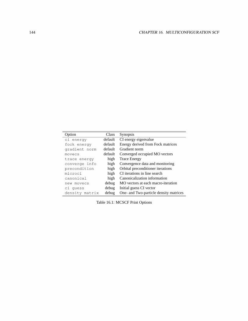
144 CHAPTER 16. MULTICONFIGURATION SCF
Option Class Synopsisci energy default CI energy eigenvaluefock energy default Energy derived from Fock matricesgradient norm default Gradient normmovecs default Converged occupied MO vectorstrace energy high Trace Energyconverge info high Convergence data and monitoringprecondition high Orbital preconditioner iterationsmicroci high CI iterations in line searchcanonical high Canonicalization informationnew movecs debug MO vectors at each macro-iterationci guess debug Initial guess CI vectordensity matrix debug One- and Two-particle density matrices
Table 16.1: MCSCF Print Options
Chapter 17
Selected CI
The selected CI module is integrated into NWChem but as yet no input module has been written. The input thusconsists of setting the appropriate variables in the database.
It is assumed that an initial SCF/MCSCF calculation has completed, and that MO vectors are available. These willbe used to perform a four-index transformation, if this has not already been performed.
17.1 Background
This is a general spin-adapted, configuration-driven CI program which can perform arbitrary CI calculations, the onlyrestriction being that all spin functions are present for each orbital occupation. CI wavefunctions may be specifiedusing a simple configuration generation program, but the prime usage is intended to be in combination with pertur-bation correction and selection of new configurations. The second-order correction (Epstein-Nesbet) to the CI energymay be computed, and at the same time configurations that interact greater than a certain threshold with the currentCI wavefunction may be chosen for inclusion in subsequent calculations. By repeating this process (typically twice isadequate) with the same threshold until no new configurations are added, the CI expansion may be made consistentwith the selection threshold, enabling tentative extrapolation to the full-CI limit.
A typical sequence of calculations is as follows:
1. Pick as an initial CI reference the previously executed SCF/MCSCF.
2. Define an initial selection threshold.
3. Determine the roots of interest in the current reference space.
4. Compute the perturbation correction and select additional configurations that interact greater than the currentthreshold.
5. Repeat steps 3 and 4.
6. Lower the threshold (a factor of 10 is common) and repeat steps 3, 4, and 5. Thefirst pass through step 4 willyield the approximately self-consistent CI and CI+PT energies from thepreviousselection threshold.
To illustrate this, below is some abbreviated output from a calculation on water in an augmented cc-PVDZ basisset with one frozen core orbital. The SCF was converged to high precision inC2v symmetry with the following input
145
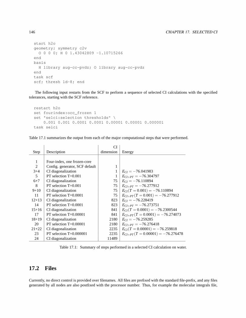
146 CHAPTER 17. SELECTED CI
start h2ogeometry; symmetry c2v
O 0 0 0; H 0 1.43042809 -1.10715266endbasis
H library aug-cc-pvdz; O library aug-cc-pvdzendtask scfscf; thresh 1d-8; end
The following input restarts from the SCF to perform a sequence of selected CI calculations with the specifiedtolerances, starting with the SCF reference.
restart h2oset fourindex:occ_frozen 1set "selci:selection thresholds" \
0.001 0.001 0.0001 0.0001 0.00001 0.00001 0.000001task selci
Table 17.1 summarizes the output from each of the major computational steps that were performed.
CIStep Description dimension Energy
1 Four-index, one frozen-core2 Config. generator, SCF default 1
3+4 CI diagonalization 1 ECI =−76.0419835 PT selection T=0.001 1 ECI+PT =−76.304797
6+7 CI diagonalization 75 ECI =−76.1108948 PT selection T=0.001 75 ECI+PT =−76.277912
9+10 CI diagonalization 75 ECI(T = 0.001) =−76.11089411 PT selection T=0.0001 75 ECI+PT(T = 0.001) =−76.277912
12+13 CI diagonalization 823 ECI =−76.22841914 PT selection T=0.0001 823 ECI+PT =−76.273751
15+16 CI diagonalization 841 ECI(T = 0.0001) =−76.230054417 PT selection T=0.00001 841 ECI+PT(T = 0.0001) =−76.274073
18+19 CI diagonalization 2180 ECI =−76.25928520 PT selection T=0.00001 2180 ECI+PT =−76.276418
21+22 CI diagonalization 2235 ECI(T = 0.00001) =−76.25981823 PT selection T=0.000001 2235 ECI+PT(T = 0.00001) =−76.27647824 CI diagonalization 11489
Table 17.1: Summary of steps performed in a selected CI calculation on water.
17.2 Files
Currently, no direct control is provided over filenames. All files are prefixed with the standard file-prefix, and any filesgenerated by all nodes are also postfixed with the processor number. Thus, for example the molecular integrals file,
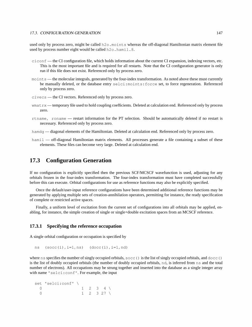
17.3. CONFIGURATION GENERATION 147
used only by process zero, might be calledh2o.moints whereas the off-diagonal Hamiltonian matrix element fileused by process number eight would be calledh2o.hamil.8 .
ciconf — the CI configuration file, which holds information about the current CI expansion, indexing vectors, etc.This is the most important file and is required for all restarts. Note that the CI configuration generator is onlyrun if this file does not exist. Referenced only by process zero.
moints — the molecular integrals, generated by the four-index transformation. As noted above these must currentlybe manually deleted, or the database entryselci:moints:force set, to force regeneration. Referencedonly by process zero.
civecs — the CI vectors. Referenced only by process zero.
wmatrx — temporary file used to hold coupling coefficients. Deleted at calculation end. Referenced only by processzero.
rtname, roname — restart information for the PT selection. Should be automatically deleted if no restart isnecessary. Referenced only by process zero.
hamdg — diagonal elements of the Hamiltonian. Deleted at calculation end. Referenced only by process zero.
hamil — off-diagonal Hamiltonian matrix elements. All processes generate a file containing a subset of theseelements. These files can become very large. Deleted at calculation end.
17.3 Configuration Generation
If no configuration is explicitly specified then the previous SCF/MCSCF wavefunction is used, adjusting for anyorbitals frozen in the four-index transformation. The four-index transformation must have completed successfullybefore this can execute. Orbital configurations for use as reference functions may also be explicitly specified.
Once the default/user-input reference configurations have been determined additional reference functions may begenerated by applying multiple sets of creation-annihilation operators, permitting for instance, the ready specificationof complete or restricted active spaces.
Finally, a uniform level of excitation from the current set of configurations into all orbitals may be applied, en-abling, for instance, the simple creation of single or single+double excitation spaces from an MCSCF reference.
17.3.1 Specifying the reference occupation
A single orbital configuration or occupation is specified by
ns (socc(i),i=1,ns) (docc(i),i=1,nd)
wherens specifies the number of singly occupied orbitals,socc() is the list of singly occupied orbitals, anddocc()is the list of doubly occupied orbitals (the number of doubly occupied orbitals,nd , is inferred fromns and the totalnumber of electrons). All occupations may be strung together and inserted into the database as a single integer arraywith name"selci:conf" . For example, the input
set "selci:conf" \0 1 2 3 4 \0 1 2 3 27 \
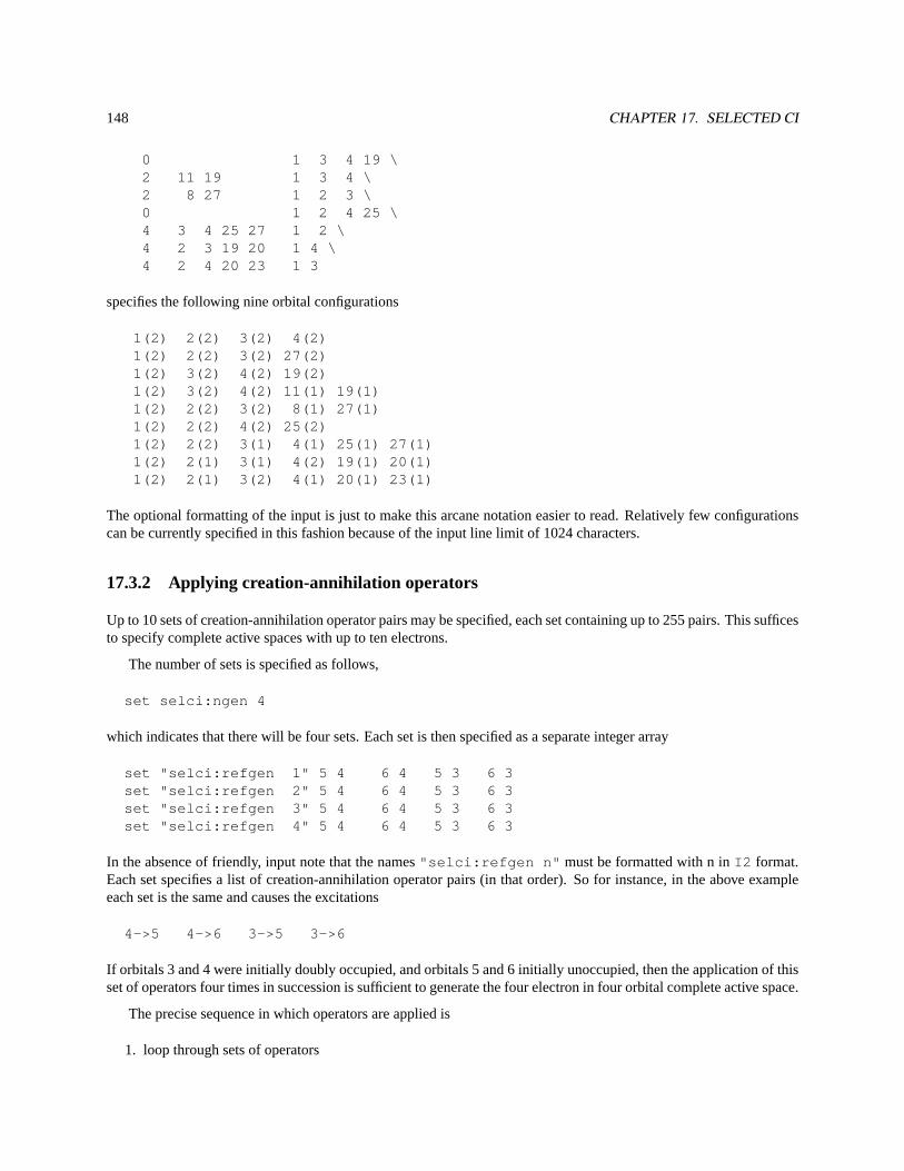
148 CHAPTER 17. SELECTED CI
0 1 3 4 19 \2 11 19 1 3 4 \2 8 27 1 2 3 \0 1 2 4 25 \4 3 4 25 27 1 2 \4 2 3 19 20 1 4 \4 2 4 20 23 1 3
specifies the following nine orbital configurations
1(2) 2(2) 3(2) 4(2)1(2) 2(2) 3(2) 27(2)1(2) 3(2) 4(2) 19(2)1(2) 3(2) 4(2) 11(1) 19(1)1(2) 2(2) 3(2) 8(1) 27(1)1(2) 2(2) 4(2) 25(2)1(2) 2(2) 3(1) 4(1) 25(1) 27(1)1(2) 2(1) 3(1) 4(2) 19(1) 20(1)1(2) 2(1) 3(2) 4(1) 20(1) 23(1)
The optional formatting of the input is just to make this arcane notation easier to read. Relatively few configurationscan be currently specified in this fashion because of the input line limit of 1024 characters.
17.3.2 Applying creation-annihilation operators
Up to 10 sets of creation-annihilation operator pairs may be specified, each set containing up to 255 pairs. This sufficesto specify complete active spaces with up to ten electrons.
The number of sets is specified as follows,
set selci:ngen 4
which indicates that there will be four sets. Each set is then specified as a separate integer array
set "selci:refgen 1" 5 4 6 4 5 3 6 3set "selci:refgen 2" 5 4 6 4 5 3 6 3set "selci:refgen 3" 5 4 6 4 5 3 6 3set "selci:refgen 4" 5 4 6 4 5 3 6 3
In the absence of friendly, input note that the names"selci:refgen n" must be formatted with n inI2 format.Each set specifies a list of creation-annihilation operator pairs (in that order). So for instance, in the above exampleeach set is the same and causes the excitations
4->5 4->6 3->5 3->6
If orbitals 3 and 4 were initially doubly occupied, and orbitals 5 and 6 initially unoccupied, then the application of thisset of operators four times in succession is sufficient to generate the four electron in four orbital complete active space.
The precise sequence in which operators are applied is
1. loop through sets of operators
17.4. NUMBER OF ROOTS 149
2. loop through reference configurations
3. loop through operators in the set
4. apply the operator to the configuration, if the result is new add it to the new list
5. end the loop over operators
6. end the loop over reference configurations
7. augment the configuration list with the new list
8. end the loop over sets of operators
17.3.3 Uniform excitation level
By default no excitation is applied to the reference configurations. If, for instance, you wanted to generate a singleexcitation CI space from the current configuration list, specify
set selci:exci 1
Any excitation level may be applied, but since the list of configurations is explicitly generated, as is the CI Hamiltonianmatrix, you will run out of disk space if you attempt to use more than a few tens of thousands of configurations.
17.4 Number of roots
By default, only one root is generated in the CI diagonalization or perturbation selection. The following requests that2 roots be generated
set selci:nroot 2
There is no imposed upper limit. If many roots are required, then, to minimize root skipping problems, it helps toperform an initial approximate diagonalization with several more roots than required, and then resetting this parameteronce satisfied that the desired states are obtained.
17.5 Accuracy of diagonalization
By default, the CI wavefunctions are converged to a residual norm of 10−6 which provides similar accuracy in theperturbation corrections to the energy, and much higher accuracy in the CI eigenvalues. This may be adjusted with
set "selci:diag tol" 1d-3
the example setting much lower precision, appropriate for the approximate diagonalization discussed in the precedingsection.
150 CHAPTER 17. SELECTED CI
17.6 Selection thresholds
When running in the selected-CI mode the program will loop through a list of selection thresholds (T), performing theCI diagonalization, computing the perturbation correction, and augmenting the CI expansion with configurations thatmake an energy lowering to any root greater thanT. The list of selection thresholds is specified as follows
set "selci:selection thresholds" \0.001 0.001 0.0001 0.0001 0.00001 0.00001 0.000001
There is no default for this parameter.
17.7 Mode
By default the program runs in"ci+davids" mode and just determines the CI eigenvectors/values in the currentconfiguration space. To perform a selected-CI with perturbation correction use the following
set selci:mode select
and remember to define the selection thresholds.
17.8 Memory requirements
No global arrays are used inside the selected-CI, though the four-index transformation can be automatically invokedand it does use GAs. The selected CI replicates inside each process
• all unique two-electron integrals in the MO basis that are non-zero by symmetry, and
• all CI information, including the CI vectors.
These large data structures are allocated on the local stack. A fatal error will result if insufficient memory is available.
17.9 Forcing regeneration of the MO integrals
When scanning a potential energy surface or optimizing a geometry the MO integrals need to be regenerated eachtime. Specify
set selci:moints:force logical .true.
to accomplish this.
17.10 Disabling update of the configuration list
When computing CI+PT energy the reference configuration list is normally updated to reflect all configurations thatinteract more than the specified threshold. This is usually desirable. But when scanning a potential energy surface or

17.11. ORBITAL LOCKING IN CI GEOMETRY OPTIMIZATION 151
optimizing a geometry the reference list must be kept fixed to keep the potential energy surface continuous and welldefined. To do this specify
set selci:update logical .false.
17.11 Orbital locking in ci geometry optimization
The selected CI wavefunction is not invariant to orbital rotations or to swapping two or more orbitals. Orbitals couldbe swapped or rotated when the geometry is changed in a geometry optimization step. The keywordlock has to be setin the SCF/MCSCF (vectors) input block to keep the orbitals in the same order throughout the geometry optimization.

152 CHAPTER 17. SELECTED CI
Chapter 18
Coupled Cluster Calculations
The NWChem coupled cluster energy module is primarily the work of Alistair Rendell and Rika Kobayashi, withcontributions from David Bernholdt, and is derived from the Titan parallel coupled cluster program.
The coupled cluster code can perform calculations with full iterative treatment of single and double excitationsand non-iterative inclusion of triple excitation effects. It is presently limited to closed-shell (RHF) references.
Note that symmetry is not used within most of the CCSD(T) code.This can have a profound impact on performancesince the speed-up from symmetry is roughly the square of the number of irreducible representations. In the absenceof symmetry, the performance of this code is competitive with other programs.
The operation of the coupled cluster code is controlled by the input block
CCSD[MAXITER <integer maxiter default 20>][THRESH <real thresh default 10^-6>][TOL2E <real tol2e default min(10^-12 , 0.01*$thresh$)>][DIISBAS <integer diisbas default 5>][FREEZE [[core] (atomic || <integer nfzc default 0>)] \
[virtual <integer nfzv default 0>]][IPRT <integer IPRT default 0>][PRINT ...][NOPRINT ...]
END
Note that the keywordCCSDis used for the input block regardless of the actual level of theory desired (specified withtheTASKdirective). The following directives are recognized within theCCSDgroup.
18.1 MAXITER— Maximum number of iterations
The maximum number of iterations is set to 20 by default. This should be quite enough for most calculations, althoughparticularly troublesome cases may require more.
MAXITER <integer maxiter default 20>
153
154 CHAPTER 18. COUPLED CLUSTER CALCULATIONS
18.2 THRESH— Convergence threshold
Controls the convergence threshold for the iterative part of the calculation. Both the RMS error in the amplitudesandthe change in energy must be less thanthresh .
THRESH <real thresh default 10^-6>
18.3 TOL2E— integral screening threshold
TOL2E <real tol2e default min(10^-12 , 0.01*$thresh$)>
The variabletol2e is used in determining the integral screening threshold for the evaluation of the energy andrelated quantities.
CAUTION!At the present time, thetol2e parameter only affects the three- and four-virtual contributions, andthe triples, all of which are done “on the fly”. The transformations used for the other parts of the code currently havea hard-wired threshold of 10−12. The default fortol2e is set to match this, and since user input can only make thethreshold smaller, setting this parameter can only make calculations take longer.
18.4 DIISBAS — DIIS subspace dimension
Specifies the maximum size of the subspace used in DIIS convergence acceleration. Note that DIIS requires theamplitudes and errors be stored for each iteration in the subspace. Obviously this can significantly increase memoryrequirements, and could force the user to reduceDIISBAS for large calculations.
Measures to alleviate this problem, including more compact storage of the quantities involved, and the possibilityof disk storage are being considered, but have not yet been implemented.
DIISBAS <integer diisbas default 5>
18.5 FREEZE— Freezing orbitals
[FREEZE [[core] (atomic || <integer nfzc default 0>)] \[virtual <integer nfzv default 0>]]
This directive is idential to that used in the MP2 module, Section 15.1.1.
18.6 IPRT — Debug printing
This directive controls the level of output from the code, mostly to facilitate debugging and the like. The larger thevalue, the more output printed. From looking at the source code, the interesting values seem to beIPRT > 5, 10, and50.
IPRT <integer IPRT default 0>
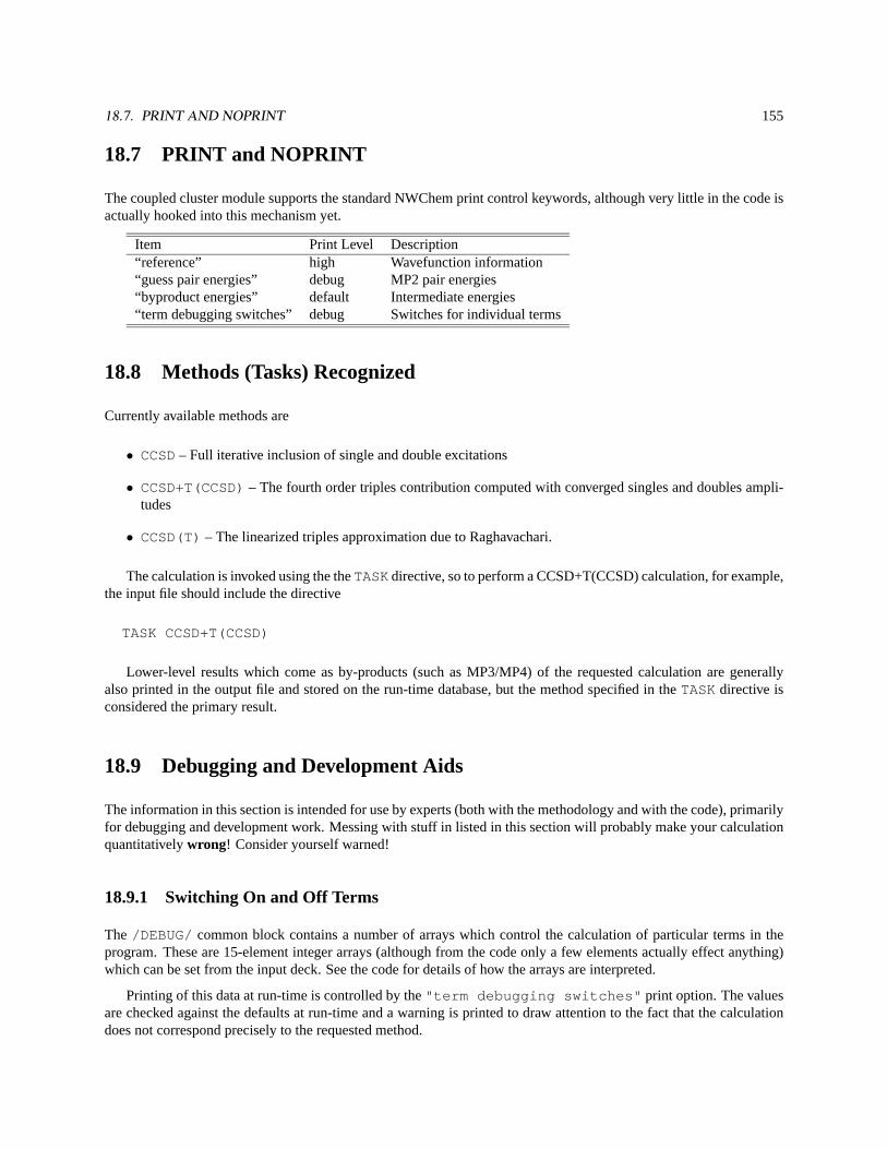
18.7. PRINT AND NOPRINT 155
18.7 PRINT and NOPRINT
The coupled cluster module supports the standard NWChem print control keywords, although very little in the code isactually hooked into this mechanism yet.
Item Print Level Description“reference” high Wavefunction information“guess pair energies” debug MP2 pair energies“byproduct energies” default Intermediate energies“term debugging switches” debug Switches for individual terms
18.8 Methods (Tasks) Recognized
Currently available methods are
• CCSD– Full iterative inclusion of single and double excitations
• CCSD+T(CCSD)– The fourth order triples contribution computed with converged singles and doubles ampli-tudes
• CCSD(T) – The linearized triples approximation due to Raghavachari.
The calculation is invoked using the theTASKdirective, so to perform a CCSD+T(CCSD) calculation, for example,the input file should include the directive
TASK CCSD+T(CCSD)
Lower-level results which come as by-products (such as MP3/MP4) of the requested calculation are generallyalso printed in the output file and stored on the run-time database, but the method specified in theTASKdirective isconsidered the primary result.
18.9 Debugging and Development Aids
The information in this section is intended for use by experts (both with the methodology and with the code), primarilyfor debugging and development work. Messing with stuff in listed in this section will probably make your calculationquantitativelywrong! Consider yourself warned!
18.9.1 Switching On and Off Terms
The /DEBUG/ common block contains a number of arrays which control the calculation of particular terms in theprogram. These are 15-element integer arrays (although from the code only a few elements actually effect anything)which can be set from the input deck. See the code for details of how the arrays are interpreted.
Printing of this data at run-time is controlled by the"term debugging switches" print option. The valuesare checked against the defaults at run-time and a warning is printed to draw attention to the fact that the calculationdoes not correspond precisely to the requested method.
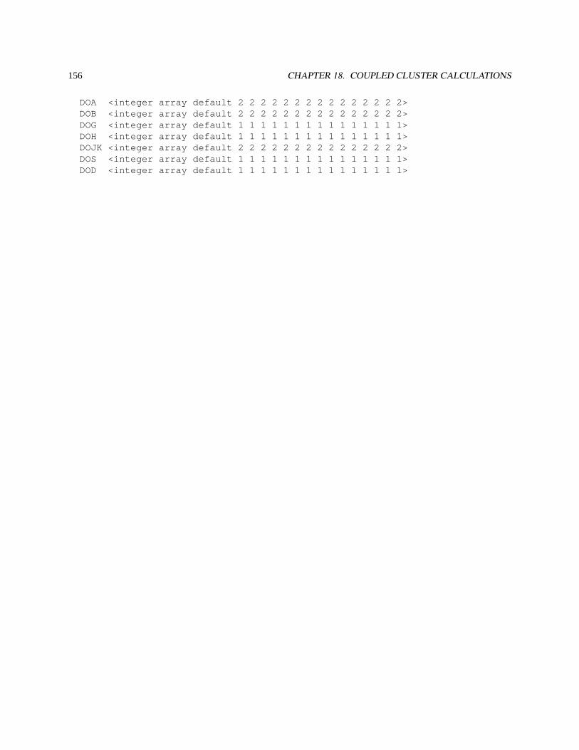
156 CHAPTER 18. COUPLED CLUSTER CALCULATIONS
DOA <integer array default 2 2 2 2 2 2 2 2 2 2 2 2 2 2 2>DOB <integer array default 2 2 2 2 2 2 2 2 2 2 2 2 2 2 2>DOG <integer array default 1 1 1 1 1 1 1 1 1 1 1 1 1 1 1>DOH <integer array default 1 1 1 1 1 1 1 1 1 1 1 1 1 1 1>DOJK <integer array default 2 2 2 2 2 2 2 2 2 2 2 2 2 2 2>DOS <integer array default 1 1 1 1 1 1 1 1 1 1 1 1 1 1 1>DOD <integer array default 1 1 1 1 1 1 1 1 1 1 1 1 1 1 1>

Chapter 19
Geometry Optimization with DRIVER
The DRIVER module is one of two drivers (see Section 20 for documentation on STEPPER) to perform a geometryoptimization function on the molecule defined by input using theGEOMETRYdirective (see Section 6). Geometry op-timization is either an energy minimization or a transition state optimization. The algorithm programmed in DRIVERis a quasi-newton optimization with line searches and approximate energy Hessian updates.
DRIVER is selected by default out of the two available modules to perform geometry optimization. In order toforce use of DRIVER (e.g., because a previous optimization used STEPPER) provide a DRIVER input block (below)— even an empty block will force use of DRIVER.
Optional input for this module is specified within the compound directive,
DRIVER(LOOSE || DEFAULT || TIGHT)GMAX <real value>GRMS <real value>XMAX <real value>XRMS <real value>
EPREC <real eprec default 1e-7>
TRUST <real trust default 0.3>SADSTP <real sadstp default 0.1>
CLEARREDOAUTOZ
INHESS <integer inhess default 0>
(MODDIR || VARDIR) <integer dir default 0>(FIRSTNEG || NOFIRSTNEG)
MAXITER <integer maxiter default 20>
BSCALE <real BSCALE default 1.0>ASCALE <real ASCALE default 0.25>TSCALE <real TSCALE default 0.1>
157
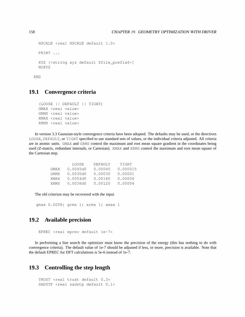
158 CHAPTER 19. GEOMETRY OPTIMIZATION WITH DRIVER
HSCALE <real HSCALE default 1.0>
PRINT ...
XYZ [<string xyz default $file_prefix$>]NOXYZ
END
19.1 Convergence criteria
(LOOSE || DEFAULT || TIGHT)GMAX <real value>GRMS <real value>XMAX <real value>XRMS <real value>
In version 3.3 Gaussian-style convergence criteria have been adopted. The defaults may be used, or the directivesLOOSE, DEFAULT, or TIGHT specified to use standard sets of values, or the individual criteria adjusted. All criteriaare in atomic units.GMAXandGRMScontrol the maximum and root mean square gradient in the coordinates beingused (Z-matrix, redundant internals, or Cartesian).XMAXandXRMScontrol the maximum and root mean square ofthe Cartesian step.
LOOSE DEFAULT TIGHTGMAX 0.0045d0 0.00045 0.000015GRMS 0.0030d0 0.00030 0.00001XMAX 0.0054d0 0.00180 0.00006XRMS 0.0036d0 0.00120 0.00004
The old criterion may be recovered with the input
gmax 0.0008; grms 1; xrms 1; xmax 1
19.2 Available precision
EPREC <real eprec default 1e-7>
In performing a line search the optimizer must know the precision of the energy (this has nothing to do withconvergence criteria). The default value of 1e-7 should be adjusted if less, or more, precision is available. Note thatthe default EPREC for DFT calculations is 5e-6 instead of 1e-7.
19.3 Controlling the step length
TRUST <real trust default 0.3>SADSTP <real sadstp default 0.1>
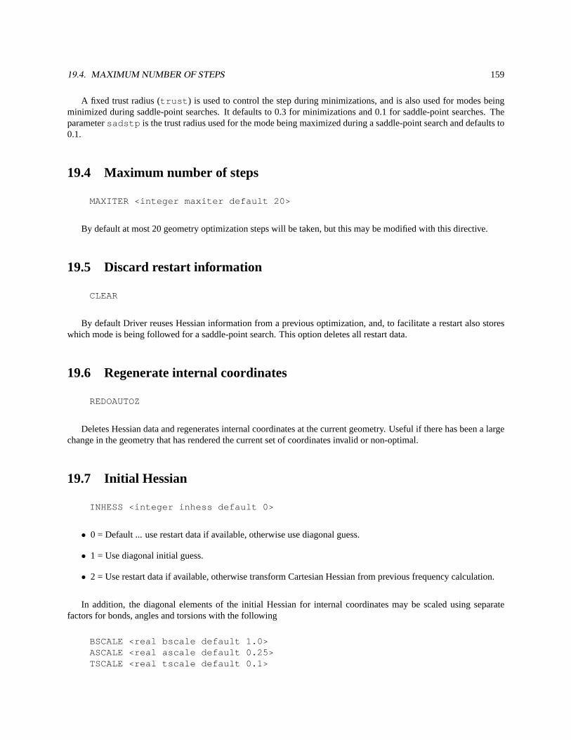
19.4. MAXIMUM NUMBER OF STEPS 159
A fixed trust radius (trust ) is used to control the step during minimizations, and is also used for modes beingminimized during saddle-point searches. It defaults to 0.3 for minimizations and 0.1 for saddle-point searches. Theparametersadstp is the trust radius used for the mode being maximized during a saddle-point search and defaults to0.1.
19.4 Maximum number of steps
MAXITER <integer maxiter default 20>
By default at most 20 geometry optimization steps will be taken, but this may be modified with this directive.
19.5 Discard restart information
CLEAR
By default Driver reuses Hessian information from a previous optimization, and, to facilitate a restart also storeswhich mode is being followed for a saddle-point search. This option deletes all restart data.
19.6 Regenerate internal coordinates
REDOAUTOZ
Deletes Hessian data and regenerates internal coordinates at the current geometry. Useful if there has been a largechange in the geometry that has rendered the current set of coordinates invalid or non-optimal.
19.7 Initial Hessian
INHESS <integer inhess default 0>
• 0 = Default ... use restart data if available, otherwise use diagonal guess.
• 1 = Use diagonal initial guess.
• 2 = Use restart data if available, otherwise transform Cartesian Hessian from previous frequency calculation.
In addition, the diagonal elements of the initial Hessian for internal coordinates may be scaled using separatefactors for bonds, angles and torsions with the following
BSCALE <real bscale default 1.0>ASCALE <real ascale default 0.25>TSCALE <real tscale default 0.1>
160 CHAPTER 19. GEOMETRY OPTIMIZATION WITH DRIVER
These values typically give a two-fold speedup over unit values, based on about 100 test cases up to 15 atoms using3-21g and 6-31g* SCF. However, if doing many optimizations on physically similar systems it may be worth finetuning these parameters.
Finally, the entire Hessian from any source may be scaled by a factor using the directive
HSCALE <real hscale default 1.0>
It might be of utility, for instance, when computing an initial Hessian using SCF to start a large MP2 optimization.The SCF vibrational modes are expected to be stiffer than the MP2, so scaling the initial Hessian by a number lessthan one might be beneficial.
19.8 Mode or variable to follow to saddle point
(MODDIR || VARDIR) <integer dir default 0>(FIRSTNEG || NOFIRSTNEG)
When searching for a transition state the program, by default, will take an initial step uphill and then do modefollowing using a fuzzy maximum overlap (the lowest eigen-mode with an overlap with the previous search directionof 0.7 times the maximum overlap is selected). Once a negative eigen-value is found, that mode is followed regardlessof overlap.
The initial uphill step is appropriate if the gradient points roughly in the direction of the saddle point, such asmight be the case if a constrained optimization was performed at the starting geometry. Alternatively, the initial searchdirection may be chosen to be along a specific internal variable (using the directiveVARDIR) or along a specific eigen-mode (usingMODDIR). Following a variable might be valuable if the initial gradient is either very small or very large.Note that the eigen-modes in the optimizer have next-to-nothing to do with the output from a frequency calculation.You can examine the eigen-modes used by the optimizer with
driver; print hvecs; end
The selection of the first negative mode is usually a good choice if the search is started in the vicinity of thetransition state and the initial search direction is satisfactory. However, sometimes the first negative mode might notbe the one of interest (e.g., transverse to the reaction direction). IfNOFIRSTNEGis specified, the code will not takethe first negative direction and will continue doing mode-following until that mode goes negative.
19.9 Optimization history as XYZ files
XYZ [<string xyz default $fileprefix>]NOXYZ
TheXYZdirective causes the geometry at each step (but not intermediate points of a line search) to be output intoseparate files in the permanent directory in XYZ format. The optional string will prefix the filename. TheNOXYZdirective turns this off.
For example, the input
driver; xyz test; end
19.10. PRINT OPTIONS 161
will cause files test-000.xyz, test-001.xyz, . . . to be created in the permanent directory.
The scriptrasmolmovie in the NWChemcontrib directory can be used to turn these into an animated GIFmovie.
19.10 Print options
The UNIX command"egrep ’^@’ < output" will extract a pretty table summarizing the optimization.
If you specify the NWChem input
scf; print none; enddriver; print low; endtask scf optimize
you’ll obtain a pleasantly terse output.
For more control, these options for the standard print directive are recognized
• debug - prints a large amount of data. Don’t use in parallel.
• high - print the search direction in internals
• default - prints geometry for each major step (not during the line search), gradient in internals (before andafter application of constraints)
• low - prints convergence and energy information. At convergence prints final geometry, change in internalsfrom initial geometry
and these specific print options
• finish (low) - print geometry data at end of calculation
• bonds (default) - print bonds at end of calculation
• angles (default) - print angles at end of calculation
• hvecs (never) - print eigen-values/vectors of the Hessian
• searchdir (high) - print the search direction in internals
• ’internal gradient’ (default) - print the gradient in internals
• sadmode (default) - print the mode being followed to the saddle point

162 CHAPTER 19. GEOMETRY OPTIMIZATION WITH DRIVER
Chapter 20
Geometry Optimization with STEPPER
The STEPPER module performs a search for critical points on the potential energy surface of the molecule definedby input using theGEOMETRYdirective (see Section 6). Since STEPPER isnot the primary geometry optimizationmodule in NWChem the compound directive is required; the DRIVER module is the default (see Section 19). Inputfor this module is specified within the compound directive,
STEPPER...
END
The presence of the STEPPER compound directive automatically turns off the default geometry optimization tooldriver. Input specified for the STEPPER module must appear in the input fileafter theGEOMETRYdirective, since itmust know the number of atoms that are to be used in the geometry optimization. In the current version of NWChem,STEPPER can be used only with geometries that are defined in Cartesian coordinates. STEPPER removes translationaland rotational components before determining the step direction (5 components for linear systems and 6 for others)using a standard Eckart algorithm. The default initial guess nuclear Hessian is the identity matrix.
The default in STEPPER is to minimize the energy as a function of the geometry with a maximum of 20 geometryoptimization iterations. When this is the desired calculation, no input is required other than the STEPPER compounddirective. However, the user also has the option of defining different tasks for the STEPPER module, and can vary thenumber of iterations and the convergence criteria from the default values. The input for these options is described inthe following sections.
20.1 MIN and TS — Minimum or transition state search
The default is for STEPPER to minimize the energy with respect to the geometry of the system. This default behaviormay be forced with the directive
MIN
STEPPER can also be used to find the transition state by following the lowest eigenvector of the nuclear Hessian.This is usually invoked by using thesaddle keyword on theTASK directive (Section 5.10), but it may also beselected by specifying the directive
TS
163
164 CHAPTER 20. GEOMETRY OPTIMIZATION WITH STEPPER
in the STEPPER input.
20.2 TRACK— Mode selection
STEPPER has the ability to “track” a specific mode during an optimization for a transition state search, the user canalso have the module track the eigenvector corresponding to a specific mode. This is done by specifying the directive
TRACK [nmode <integer nmode default 1>]
The keywordTRACKtells STEPPER to track the eigenvector corresponding to the integer value of<nmode> during atransition state walk. (Note: this input is invalid for a minimization walk since following a specific eigenvector will notnecessarily give the desired local minimum.) The step is constructed to go up in energy along thenmode eigenvectorand down in all other degrees of freedom.
20.3 MAXITER— Maximum number of steps
In most applications, 20 stepper iterations will be sufficient to obtain the energy minimization. However, the user hasthe option of specifying the maximum number of iterations allowed, using the input line,
MAXITER <integer maxiter default 20>
The value specified for the integer<maxiter> defines the maximum number of geometry optimization steps. Thegeometry optimization will restart automatically.
20.4 TRUST— Trust radius
The size of steps that can be taken in STEPPER is controlled by the trust radius which has a default value of 0.1.Steps are constrained to be no larger than the trust radius. The user has the option of overriding this default using thekeywordTRUST, with the following input line,
TRUST <real radius default 0.1>
The larger the value specified for the variableradius , the larger the steps that can be taken by STEPPER.Experience has shown that for larger systems (i.e., those with 20 or more atoms), a value of 0.5, or greater, usuallyshould be entered for<radius> .
20.5 CONVGGM, CONVGGand CONVGE— Convergence criteria
Three convergence criteria can be specified explicitly for the STEPPER calculations. The keywordCONVGGMallowsthe user to specify the convergence tolerance for the largest component of the gradient. This is the primary convergencecriterion, as per the default settings, although all three criteria are in effect. this default setting is consistent with theother optimizer module DRIVER. The input line forCONVGGMhas the following form,
CONVGGM <real convggm default 8.0d-04>
20.6. BACKSTEPPING IN STEPPER 165
The keywordCONVGGallows the user to specify the convergence tolerance for the gradient norm for all degrees offreedom. The input line is of the following form,
CONVGG <real convgg default 1.0d-02>
The entry for the real variable<convgg> should be approximately equal to the square root of the energy convergencetolerance.
The energy convergence tolerance is the convergence criterion for the energy difference in the geometry optimiza-tion in STEPPER. It can be specified by input using a line of the following form,
CONVGE <real convge default 1.0d-04>
20.6 Backstepping in Stepper
If a step taken during the optimization is too large (e.g., the step causes the energy to go up for a minimization ordown for a transition state search), the STEPPER optimizer will automatically “backstep” and correct the step basedon information prior to the faulty step. If you have an optimization that “backsteps” frequently then the initial trustradius should most likely be decreased.
20.7 Initial Nuclear Hessian Options
Stepper uses a modified Fletcher-Powell algorithm to find the transition state or energy minimum on the potentialenergy hypersurface. There are two files left in the user’s permanent directory that are used to provide an initialhessian to the critical point search algorithm. If these files do not exist then the default is to use a unit matrix as theinitial hessian. Once Stepper executes it generates a binary dump file by the name ofname.stpr41 which willbe used on all subsequent stepper runs and modified with the current updated hessian. The default file prefix is the“name” that is used (c.f., 5.1). It also stores the information for the last valid step in case the algorithm must take a“backstep” (c.f., 20.6). This file is the working data store for all stepper-based optimizations. This file is never deletedby default and is thefirst source of an initial hessian. The second source of an inital hessian is an ascii file that containsthe lower triangular values of the initial hessian. This is stored in filename.hess , where “name” is again the defaultfile prefix. This is thesecondsource of an initial hessian and is the method used to incorporate an initial hessian fromany other source (e.g., anotherab initio code, a molecular mechanics code, etc.,). To get a decent starting hessian at agiven point you can use the task specificationtask scf hessian , with a smaller basis set, which will by defaultgenerate thename.hess file. Then you may define your basis set of choice and proceed with the optimization youdesire.1
1If you have done a geometry optimization and hessian generation in the same input deck using a small basis set, you must make sure you deletethename.stpr41 file since stepper will by default use that hessian and not the one in thename.hess file

166 CHAPTER 20. GEOMETRY OPTIMIZATION WITH STEPPER
Chapter 21
Hybrid Calculations with ONIOM
ONIOM is the hybrid method of Morokuma and co-workers that enables different levels of theory to be applied todifferent parts of a molecule/system and combined to produce a consistent energy expression. The objective is toperform a high-level calculation on just a small part of the system and to include the effects of the remainder at lowerlevels of theory, with the end result being of similar accuracy to a high-level calculation on the full system.
1. M. Svensson, S. Humbel, R.D.J. Froese, T. Mastubara, S. Sieber and K. Morokuma, J. Phys. Chem, 100, 1996,p19357.
2. S. Dapprich, I. Komaromi, K.S. Byun, K. Morokuma and M.J. Frisch, J. Mol. Struct (Theochem), 461-462,1999, p1-21.
3. R.D.J. Froese and K. Morokuma in “Encylopedia of Computational Chemistry,” volume 2, p1244-1257, (ed. P.von Rague Schleyer, John Wiley and Sons, Chichester, Sussex, 1998).
The NWChem ONIOM module implements two- and three-layer ONIOM models for use in energy, gradient,geometry optimization, and vibrational frequency calculations with any of the pure quantum mechanical methodswithin NWChem. At the present time, it is not possible to perform ONIOM calculations with either solvation modelsor classical force fields. Nor is it yet possible to compute properties except as derivatives of the total energy.
Using the terminology of Morokuma et al., the full molecular geometry including all atoms is referred to as the“real” geometry and it is treated using a “low”-level of theory. A subset of these atoms (referred to as the “model”geometry) are treated using both the “low”-level and a “high”-level of theory. A three-layer model also introduces an“intermediate” model geometry and a “medium” level of theory.
The two-layer model requires a high and low level of theory and a real and model molecular geometry. The energyat the high-level of theory for the real geometry is estimated as
E(High,Real) = E(Low,Real) + [E(High,Model) - E(Low,Model)].
The three-layer model requires high, medium and low levels of theory, and real, intermediate and model geometriesand the corresponding energy estimate is
E(High,Real) = E(Low,Real) + [E(High,Model) - E(Medium,Model)]+ [E(Medium,Inter) - E(Low,Inter)].
When does ONIOM work well? The approximation for a two-layer model will be good if
167
168 CHAPTER 21. HYBRID CALCULATIONS WITH ONIOM
• the model system includes the interactions that dominate the energy difference being computed and the high-level of theory describes these to the required precision, and
• the interactions between the model and the rest of the real system (substitution effects) are described to sufficientaccuracy at the lower level of theory.
ONIOM is used to compute energy differences and the absolute energies are not all that meaningful even though theyare well defined. Due to cancellation of errors, ONIOM actually works better than you might expect, but a poorlydesigned calculation can yield very bad results. Please read and heed the caution at the end of the article by Dapprichet al.
The input options are as follows
ONIOMHIGH <string theory> [basis <string basis default "ao basis">] \
[ecp <string ecp>] [input <string input>][MEDIUM <string theory> [basis <string basis default "ao basis">] \
[ecp <string ecp>] [input <string input>]]LOW <string theory> [basis <string basis default "ao basis">] \
[ecp <string ecp>] [input <string input>]MODEL <integer natoms> [charge <double charge>] \
[<integer i1 j1> <real g1> [<string tag1>] ...][INTER <integer natoms> [charge <double charge>] \
[<integer i1 j1> <real g1> [<string tag1>] ...]][VECTORS [low-real <string mofile>] [low-model <string mofile>] \
[high-model <string mofile>] [medium-model <string mofile]\[medium-inter <string mofile>] [low-inter <string mofile>]]
[PRINT ...][NOPRINT ...]
END
which are described in detail below.
For better validation of user input, theHIGH, LOWandMODELdirectives must always be specified. If the one oftheMEDIUMor INTER directives are specified, then so must the other.
21.1 Real, model and intermediate geometries
The geometry and total charge of the full or real system should be specified as normal using the geometry directive(see Section 6). IfNmodel of the atoms are to be included in the model system, then these should be specified firstin the geometry. Similarly, in a three-layer calculation, if there areNinter atoms to be included in the intermediatesystem, then these should also be arranged together at the beginning of the geometry. The implict assumption is thatthe model system is a subset of the intermediate system which is a subset of the real system. The number of atoms tobe included in the model and intemediate systems are specified using theMODELandINTER directives. Optionally,the total charge of the model and intermediate systems may be adjusted. The default is that all three systems have thesame total charge.
Example 1. A two-layer calculation onK+(H2O) taking the potassium ion as the model system. Note that nobonds are broken so no link atoms are introduced. The real geometry would be specified with potassium (the model)first.
21.1. REAL, MODEL AND INTERMEDIATE GEOMETRIES 169
geometry autosymK 0 0.00 1.37O 0 0.00 -1.07H 0 -0.76 -1.68H 0 0.76 -1.68
end
and the following directive in the ONIOM input block indicates that one atom (implicitly the first in the geometry) isin the model system
model 1
21.1.1 Link atoms
Link atoms for bonds spanning two regions are automatically generated from the bond information. The additionalparameters on theMODELandINTER directives describe the broken bonds including scale factors for placement ofthe link atom and, optionally, the type of link atom. The type of link atom defaults to hydrogen, but any type maybe specified (actually here you are specifying a geometry tag which is used to associate a geometrical center with anatom type and basis sets, etc.. See section 6.3). For each broken bond specify the numbers of the two atoms (i and j),the scale factor (g) and optionally the tag of the link atom. Link atoms are placed along the vector connecting the thefirst to the second atom of the bond according to the equation
Rlink = (1−g)R1 +g∗R2
whereg is the scale factor. If the scale factor is one, then the link atom is placed where the second atom was. Moreusually, the scale factor is less than one, in which case the link atom is placed between the original two atoms. Thescale factor should be chosen so that the link atom (usually hydrogen) is placed near its equilibrium bond length fromthe model atom. E.g., when breaking a single carbon-carbon bond (typical length 1.528 Angstrøms) using a hydrogenlink atom we will want a carbon-hydrogen bond length of about 1.084 Angstrøms, so the scale factor should be chosenas 1.084/1.528≈ 0.709.
Example 2. A calculation on acetaldehyde (H3C−CHO) using aldehyde (H−CHO) as the model system. Thecovalent bond between the two carbon atoms is broken and a link atom must be introduced to replace the methyl group.The link atom is automatically generated — all you need to do is specify the atoms in the model system that are alsoin the real system (hereCHO) and the broken bonds. Here is the geometry of acetaldehyde with theCHOof aldehydefirst
geometryC -0.383 0.288 0.021H -1.425 0.381 0.376O 0.259 1.263 -0.321
H 0.115 -1.570 1.007H -0.465 -1.768 -0.642H 1.176 -1.171 -0.352C 0.152 -1.150 0.005
end
There are three atoms (the first three) of the real geometry included in the model geometry, and we are breaking thebond between atoms 1 and 7, replacing atom 7 with a hydrogen link atom. This is all accomplished by the directive
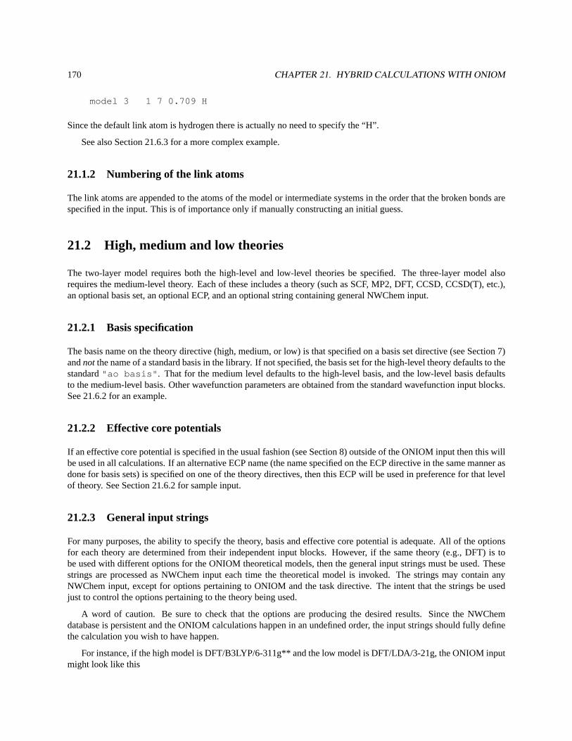
170 CHAPTER 21. HYBRID CALCULATIONS WITH ONIOM
model 3 1 7 0.709 H
Since the default link atom is hydrogen there is actually no need to specify the “H”.
See also Section 21.6.3 for a more complex example.
21.1.2 Numbering of the link atoms
The link atoms are appended to the atoms of the model or intermediate systems in the order that the broken bonds arespecified in the input. This is of importance only if manually constructing an initial guess.
21.2 High, medium and low theories
The two-layer model requires both the high-level and low-level theories be specified. The three-layer model alsorequires the medium-level theory. Each of these includes a theory (such as SCF, MP2, DFT, CCSD, CCSD(T), etc.),an optional basis set, an optional ECP, and an optional string containing general NWChem input.
21.2.1 Basis specification
The basis name on the theory directive (high, medium, or low) is that specified on a basis set directive (see Section 7)andnot the name of a standard basis in the library. If not specified, the basis set for the high-level theory defaults to thestandard"ao basis" . That for the medium level defaults to the high-level basis, and the low-level basis defaultsto the medium-level basis. Other wavefunction parameters are obtained from the standard wavefunction input blocks.See 21.6.2 for an example.
21.2.2 Effective core potentials
If an effective core potential is specified in the usual fashion (see Section 8) outside of the ONIOM input then this willbe used in all calculations. If an alternative ECP name (the name specified on the ECP directive in the same manner asdone for basis sets) is specified on one of the theory directives, then this ECP will be used in preference for that levelof theory. See Section 21.6.2 for sample input.
21.2.3 General input strings
For many purposes, the ability to specify the theory, basis and effective core potential is adequate. All of the optionsfor each theory are determined from their independent input blocks. However, if the same theory (e.g., DFT) is tobe used with different options for the ONIOM theoretical models, then the general input strings must be used. Thesestrings are processed as NWChem input each time the theoretical model is invoked. The strings may contain anyNWChem input, except for options pertaining to ONIOM and the task directive. The intent that the strings be usedjust to control the options pertaining to the theory being used.
A word of caution. Be sure to check that the options are producing the desired results. Since the NWChemdatabase is persistent and the ONIOM calculations happen in an undefined order, the input strings should fully definethe calculation you wish to have happen.
For instance, if the high model is DFT/B3LYP/6-311g** and the low model is DFT/LDA/3-21g, the ONIOM inputmight look like this
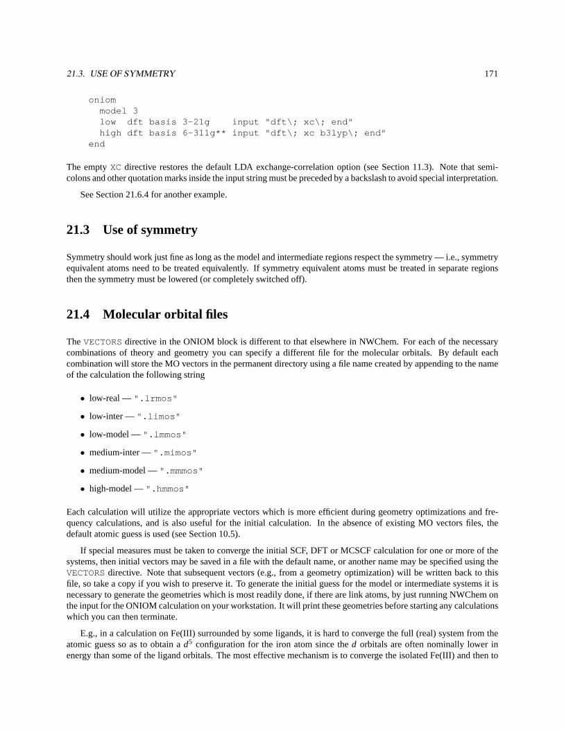
21.3. USE OF SYMMETRY 171
oniommodel 3low dft basis 3-21g input "dft\; xc\; end"high dft basis 6-311g** input "dft\; xc b3lyp\; end"
end
The emptyXC directive restores the default LDA exchange-correlation option (see Section 11.3). Note that semi-colons and other quotation marks inside the input string must be preceded by a backslash to avoid special interpretation.
See Section 21.6.4 for another example.
21.3 Use of symmetry
Symmetry should work just fine as long as the model and intermediate regions respect the symmetry — i.e., symmetryequivalent atoms need to be treated equivalently. If symmetry equivalent atoms must be treated in separate regionsthen the symmetry must be lowered (or completely switched off).
21.4 Molecular orbital files
TheVECTORSdirective in the ONIOM block is different to that elsewhere in NWChem. For each of the necessarycombinations of theory and geometry you can specify a different file for the molecular orbitals. By default eachcombination will store the MO vectors in the permanent directory using a file name created by appending to the nameof the calculation the following string
• low-real —".lrmos"
• low-inter — ".limos"
• low-model —".lmmos"
• medium-inter —".mimos"
• medium-model —".mmmos"
• high-model —".hmmos"
Each calculation will utilize the appropriate vectors which is more efficient during geometry optimizations and fre-quency calculations, and is also useful for the initial calculation. In the absence of existing MO vectors files, thedefault atomic guess is used (see Section 10.5).
If special measures must be taken to converge the initial SCF, DFT or MCSCF calculation for one or more of thesystems, then initial vectors may be saved in a file with the default name, or another name may be specified using theVECTORSdirective. Note that subsequent vectors (e.g., from a geometry optimization) will be written back to thisfile, so take a copy if you wish to preserve it. To generate the initial guess for the model or intermediate systems it isnecessary to generate the geometries which is most readily done, if there are link atoms, by just running NWChem onthe input for the ONIOM calculation on your workstation. It will print these geometries before starting any calculationswhich you can then terminate.
E.g., in a calculation on Fe(III) surrounded by some ligands, it is hard to converge the full (real) system from theatomic guess so as to obtain ad5 configuration for the iron atom since thed orbitals are often nominally lower inenergy than some of the ligand orbitals. The most effective mechanism is to converge the isolated Fe(III) and then to
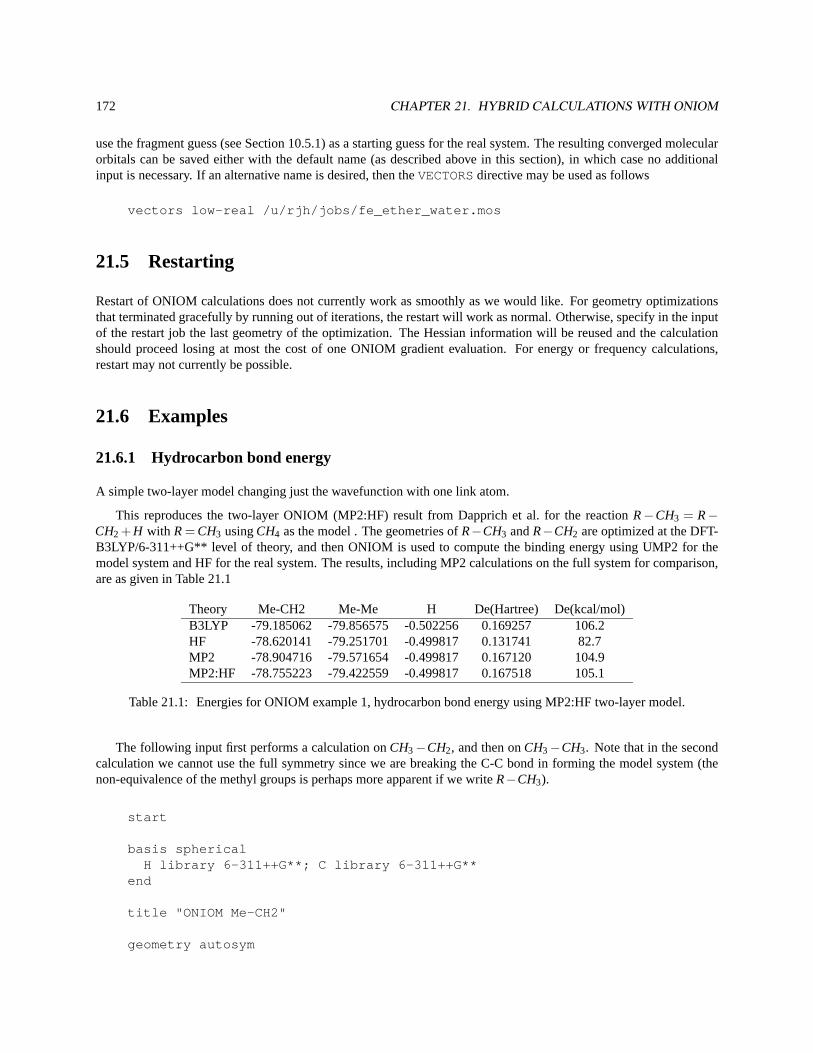
172 CHAPTER 21. HYBRID CALCULATIONS WITH ONIOM
use the fragment guess (see Section 10.5.1) as a starting guess for the real system. The resulting converged molecularorbitals can be saved either with the default name (as described above in this section), in which case no additionalinput is necessary. If an alternative name is desired, then theVECTORSdirective may be used as follows
vectors low-real /u/rjh/jobs/fe_ether_water.mos
21.5 Restarting
Restart of ONIOM calculations does not currently work as smoothly as we would like. For geometry optimizationsthat terminated gracefully by running out of iterations, the restart will work as normal. Otherwise, specify in the inputof the restart job the last geometry of the optimization. The Hessian information will be reused and the calculationshould proceed losing at most the cost of one ONIOM gradient evaluation. For energy or frequency calculations,restart may not currently be possible.
21.6 Examples
21.6.1 Hydrocarbon bond energy
A simple two-layer model changing just the wavefunction with one link atom.
This reproduces the two-layer ONIOM (MP2:HF) result from Dapprich et al. for the reactionR−CH3 = R−CH2 + H with R= CH3 usingCH4 as the model . The geometries ofR−CH3 andR−CH2 are optimized at the DFT-B3LYP/6-311++G** level of theory, and then ONIOM is used to compute the binding energy using UMP2 for themodel system and HF for the real system. The results, including MP2 calculations on the full system for comparison,are as given in Table 21.1
Theory Me-CH2 Me-Me H De(Hartree) De(kcal/mol)B3LYP -79.185062 -79.856575 -0.502256 0.169257 106.2HF -78.620141 -79.251701 -0.499817 0.131741 82.7MP2 -78.904716 -79.571654 -0.499817 0.167120 104.9MP2:HF -78.755223 -79.422559 -0.499817 0.167518 105.1
Table 21.1: Energies for ONIOM example 1, hydrocarbon bond energy using MP2:HF two-layer model.
The following input first performs a calculation onCH3−CH2, and then onCH3−CH3. Note that in the secondcalculation we cannot use the full symmetry since we are breaking the C-C bond in forming the model system (thenon-equivalence of the methyl groups is perhaps more apparent if we writeR−CH3).
start
basis sphericalH library 6-311++G**; C library 6-311++G**
end
title "ONIOM Me-CH2"
geometry autosym
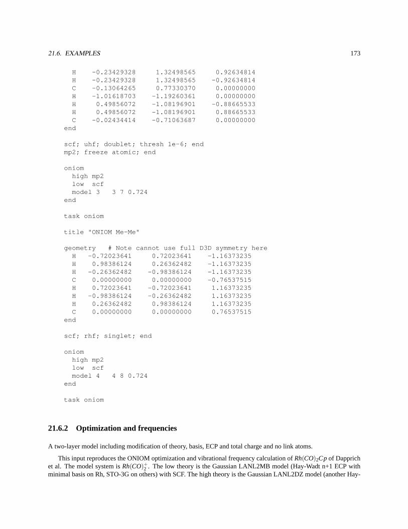
21.6. EXAMPLES 173
H -0.23429328 1.32498565 0.92634814H -0.23429328 1.32498565 -0.92634814C -0.13064265 0.77330370 0.00000000H -1.01618703 -1.19260361 0.00000000H 0.49856072 -1.08196901 -0.88665533H 0.49856072 -1.08196901 0.88665533C -0.02434414 -0.71063687 0.00000000
end
scf; uhf; doublet; thresh 1e-6; endmp2; freeze atomic; end
oniomhigh mp2low scfmodel 3 3 7 0.724
end
task oniom
title "ONIOM Me-Me"
geometry # Note cannot use full D3D symmetry hereH -0.72023641 0.72023641 -1.16373235H 0.98386124 0.26362482 -1.16373235H -0.26362482 -0.98386124 -1.16373235C 0.00000000 0.00000000 -0.76537515H 0.72023641 -0.72023641 1.16373235H -0.98386124 -0.26362482 1.16373235H 0.26362482 0.98386124 1.16373235C 0.00000000 0.00000000 0.76537515
end
scf; rhf; singlet; end
oniomhigh mp2low scfmodel 4 4 8 0.724
end
task oniom
21.6.2 Optimization and frequencies
A two-layer model including modification of theory, basis, ECP and total charge and no link atoms.
This input reproduces the ONIOM optimization and vibrational frequency calculation ofRh(CO)2Cpof Dapprichet al. The model system isRh(CO)+
2 . The low theory is the Gaussian LANL2MB model (Hay-Wadt n+1 ECP withminimal basis on Rh, STO-3G on others) with SCF. The high theory is the Gaussian LANL2DZ model (another Hay-
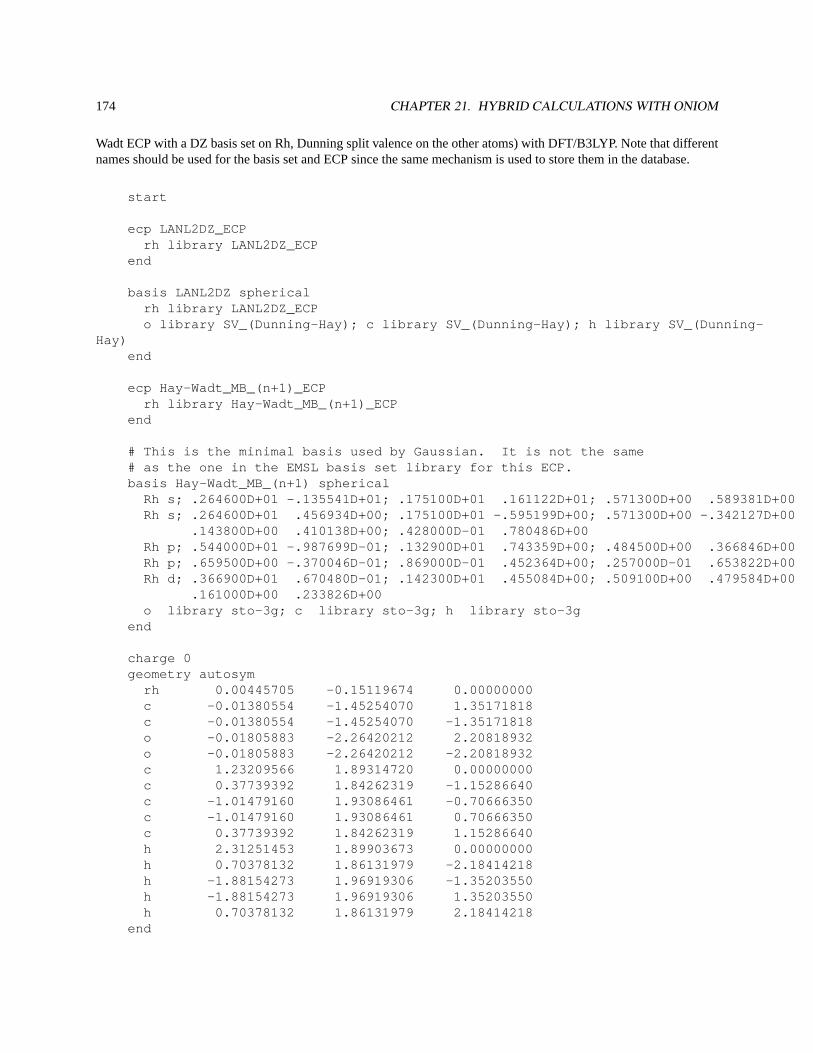
174 CHAPTER 21. HYBRID CALCULATIONS WITH ONIOM
Wadt ECP with a DZ basis set on Rh, Dunning split valence on the other atoms) with DFT/B3LYP. Note that differentnames should be used for the basis set and ECP since the same mechanism is used to store them in the database.
start
ecp LANL2DZ_ECPrh library LANL2DZ_ECP
end
basis LANL2DZ sphericalrh library LANL2DZ_ECPo library SV_(Dunning-Hay); c library SV_(Dunning-Hay); h library SV_(Dunning-
Hay)end
ecp Hay-Wadt_MB_(n+1)_ECPrh library Hay-Wadt_MB_(n+1)_ECP
end
# This is the minimal basis used by Gaussian. It is not the same# as the one in the EMSL basis set library for this ECP.basis Hay-Wadt_MB_(n+1) spherical
Rh s; .264600D+01 -.135541D+01; .175100D+01 .161122D+01; .571300D+00 .589381D+00Rh s; .264600D+01 .456934D+00; .175100D+01 -.595199D+00; .571300D+00 -.342127D+00
.143800D+00 .410138D+00; .428000D-01 .780486D+00Rh p; .544000D+01 -.987699D-01; .132900D+01 .743359D+00; .484500D+00 .366846D+00Rh p; .659500D+00 -.370046D-01; .869000D-01 .452364D+00; .257000D-01 .653822D+00Rh d; .366900D+01 .670480D-01; .142300D+01 .455084D+00; .509100D+00 .479584D+00
.161000D+00 .233826D+00o library sto-3g; c library sto-3g; h library sto-3g
end
charge 0geometry autosym
rh 0.00445705 -0.15119674 0.00000000c -0.01380554 -1.45254070 1.35171818c -0.01380554 -1.45254070 -1.35171818o -0.01805883 -2.26420212 2.20818932o -0.01805883 -2.26420212 -2.20818932c 1.23209566 1.89314720 0.00000000c 0.37739392 1.84262319 -1.15286640c -1.01479160 1.93086461 -0.70666350c -1.01479160 1.93086461 0.70666350c 0.37739392 1.84262319 1.15286640h 2.31251453 1.89903673 0.00000000h 0.70378132 1.86131979 -2.18414218h -1.88154273 1.96919306 -1.35203550h -1.88154273 1.96919306 1.35203550h 0.70378132 1.86131979 2.18414218
end
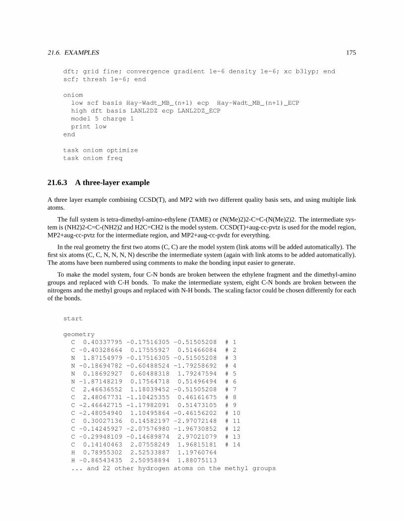
21.6. EXAMPLES 175
dft; grid fine; convergence gradient 1e-6 density 1e-6; xc b3lyp; endscf; thresh 1e-6; end
oniomlow scf basis Hay-Wadt_MB_(n+1) ecp Hay-Wadt_MB_(n+1)_ECPhigh dft basis LANL2DZ ecp LANL2DZ_ECPmodel 5 charge 1print low
end
task oniom optimizetask oniom freq
21.6.3 A three-layer example
A three layer example combining CCSD(T), and MP2 with two different quality basis sets, and using multiple linkatoms.
The full system is tetra-dimethyl-amino-ethylene (TAME) or (N(Me)2)2-C=C-(N(Me)2)2. The intermediate sys-tem is (NH2)2-C=C-(NH2)2 and H2C=CH2 is the model system. CCSD(T)+aug-cc-pvtz is used for the model region,MP2+aug-cc-pvtz for the intermediate region, and MP2+aug-cc-pvdz for everything.
In the real geometry the first two atoms (C, C) are the model system (link atoms will be added automatically). Thefirst six atoms (C, C, N, N, N, N) describe the intermediate system (again with link atoms to be added automatically).The atoms have been numbered using comments to make the bonding input easier to generate.
To make the model system, four C-N bonds are broken between the ethylene fragment and the dimethyl-aminogroups and replaced with C-H bonds. To make the intermediate system, eight C-N bonds are broken between thenitrogens and the methyl groups and replaced with N-H bonds. The scaling factor could be chosen differently for eachof the bonds.
start
geometryC 0.40337795 -0.17516305 -0.51505208 # 1C -0.40328664 0.17555927 0.51466084 # 2N 1.87154979 -0.17516305 -0.51505208 # 3N -0.18694782 -0.60488524 -1.79258692 # 4N 0.18692927 0.60488318 1.79247594 # 5N -1.87148219 0.17564718 0.51496494 # 6C 2.46636552 1.18039452 -0.51505208 # 7C 2.48067731 -1.10425355 0.46161675 # 8C -2.46642715 -1.17982091 0.51473105 # 9C -2.48054940 1.10495864 -0.46156202 # 10C 0.30027136 0.14582197 -2.97072148 # 11C -0.14245927 -2.07576980 -1.96730852 # 12C -0.29948109 -0.14689874 2.97021079 # 13C 0.14140463 2.07558249 1.96815181 # 14H 0.78955302 2.52533887 1.19760764H -0.86543435 2.50958894 1.88075113... and 22 other hydrogen atoms on the methyl groups
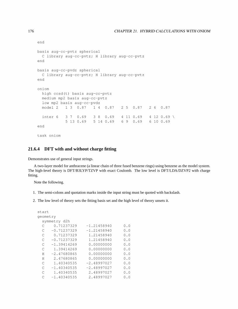
176 CHAPTER 21. HYBRID CALCULATIONS WITH ONIOM
end
basis aug-cc-pvtz sphericalC library aug-cc-pvtz; H library aug-cc-pvtz
end
basis aug-cc-pvdz sphericalC library aug-cc-pvtz; H library aug-cc-pvtz
end
oniomhigh ccsd(t) basis aug-cc-pvtzmedium mp2 basis aug-cc-pvtzlow mp2 basis aug-cc-pvdzmodel 2 1 3 0.87 1 4 0.87 2 5 0.87 2 6 0.87
inter 6 3 7 0.69 3 8 0.69 4 11 0.69 4 12 0.69 \5 13 0.69 5 14 0.69 6 9 0.69 6 10 0.69
end
task oniom
21.6.4 DFT with and without charge fitting
Demonstrates use of general input strings.
A two-layer model for anthracene (a linear chain of three fused benzene rings) using benzene as the model system.The high-level theory is DFT/B3LYP/TZVP with exact Coulomb. The low level is DFT/LDA/DZVP2 with chargefitting.
Note the following.
1. The semi-colons and quotation marks inside the input string must be quoted with backslash.
2. The low level of theory sets the fitting basis set and the high level of theory unsets it.
startgeometry
symmetry d2hC 0.71237329 -1.21458940 0.0C -0.71237329 -1.21458940 0.0C 0.71237329 1.21458940 0.0C -0.71237329 1.21458940 0.0C -1.39414269 0.00000000 0.0C 1.39414269 0.00000000 0.0H -2.47680865 0.00000000 0.0H 2.47680865 0.00000000 0.0C 1.40340535 -2.48997027 0.0C -1.40340535 -2.48997027 0.0C 1.40340535 2.48997027 0.0C -1.40340535 2.48997027 0.0
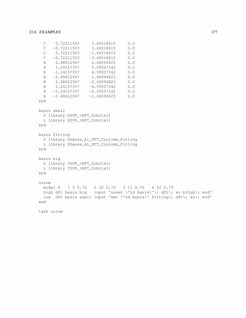
21.6. EXAMPLES 177
C 0.72211503 3.64518615 0.0C -0.72211503 3.64518615 0.0C 0.72211503 -3.64518615 0.0C -0.72211503 -3.64518615 0.0H 2.48612947 2.48094825 0.0H 1.24157357 4.59507342 0.0H -1.24157357 4.59507342 0.0H -2.48612947 2.48094825 0.0H 2.48612947 -2.48094825 0.0H 1.24157357 -4.59507342 0.0H -1.24157357 -4.59507342 0.0H -2.48612947 -2.48094825 0.0
end
basis smallh library DZVP_(DFT_Orbital)c library DZVP_(DFT_Orbital)
end
basis fittingh library DGauss_A1_DFT_Coulomb_Fittingc library DGauss_A1_DFT_Coulomb_Fitting
end
basis bigh library TZVP_(DFT_Orbital)c library TZVP_(DFT_Orbital)
end
oniommodel 8 1 9 0.75 2 10 0.75 3 11 0.75 4 12 0.75high dft basis big input "unset \"cd basis\"\; dft\; xc b3lyp\; end"low dft basis small input "set \"cd basis\" fitting\; dft\; xc\; end"
end
task oniom

178 CHAPTER 21. HYBRID CALCULATIONS WITH ONIOM
Chapter 22
Vibrational frequencies
The nuclear hessian which is used to compute the vibrational frequencies can be computed by finite difference for anyab initio wave-function that has analytic gradients. The appropriate nuclear hessian generation algorithm is chosenbased on the user input whenTASK <theory> frequencies is the task directive.
The vibrational package was integrated from the Utah Messkit and can use any nuclear hessian generated fromthe driver routines, finite difference routines or any analytic hessian modules. There is no required input for the“VIB” package. VIB computes the Infra Red frequencies and intensities1 for the computed nuclear hessian and the“projected” nuclear hessian. The VIB module projects out the translations and rotations of the nuclear hessian usingthe standard Eckart projection algorithm. It also computes the zero point energy for the molecular system based onthe frequencies obtained from the projected hessian.
The default mass of each atom is used unless an alternative mass is provided via the geometry input, (c.f., 6)or redefined using the vibrational module input. The default mass is the mass of the most abundant isotope of eachelement.2 If the abundance was roughly equal, the mass of the isotope with the longest half life was used.
22.1 Vibrational Module Input
All input for the Vibrational Module is optional since the default definitions will compute the frequencies and IRintensities3. The generic module input can begin withvib , freq , frequency and has the form:
{freq || vib || frequency}reuse [<string> hessian_filename]mass <integer> lexical_index <real> new_massmass <string> tag_identifier <real> new_massanimate [<real> step_size_for_animation]
end
1Intensities are only computed if the dipole derivatives are available; these are computed by default for most methods that use the finite differencedriver routines
2c.f., "The Elements" by John Emsley, Oxford University Press, (C) 1989, ISBN 0-19-855237-8.3The geometry specification at the point where the hessian is computed must be the default “geometry” on the current run-time-data-base for
the projection to work properly.
179
180 CHAPTER 22. VIBRATIONAL FREQUENCIES
22.1.1 Hessian File Reuse
By default thetask <theory> frequencies directive will recompute the hessian. To reuse the previouslycomputed hessian you need only specifyreuse in the module input block. If you have stored the hessian in analternate place you may redirect the reuse directive to that file by specifying the path to that file.
reuse /path_to_hessian_file
This will reuse your saved Hessian data but one caveat is that the geometry specification at the point where the hessianis computed must be the default “geometry” on the current run-time-data-base for the projection to work properly.
22.1.2 Redefining Masses of Elements
You may also modify the mass of a specific center or a group of centers via the input.
To modify the mass of a specific center you can simply use:
mass 3 4.00260324
which will set the mass of center 3 to 4.00260324 AMUs. The lexical index of centers is determined by the geometryobject.
To modify all Hydrogen atoms in a molecule you may use the tag based mechanism:
mass hydrogen 2.014101779
The mass redefinitions always start with the default masses and change the masses in the order given in the input.Care must be taken to change the masses properly. For example, if you want all hydrogens to have the mass ofDeuterium and the third hydrogen (which is the 6th atomic center) to have the mass of Tritium you must set theDeuterium masses first with the tag based mechanism and then set the 6th center’s mass to that of Tritium using thelexical center index mechanism.
The mass redefinitions are not fully persistent on the run-time-data-base. Each input block that redefines masseswill invalidate the mass definitions of the previous input block. For example,
freqreusemass hydrogen 2.014101779
endtask scf frequenciesfreq
reusemass oxygen 17.9991603
endtask scf frequencies
will use the new mass for all hydrogens in the first frequency analysis. The mass of the oxygen atoms will be redefinedin the second frequency analysis but the hydrogen atoms will use the default mass. To get a modified oxygen andhydrogen analysis you would have to use:
freq
22.1. VIBRATIONAL MODULE INPUT 181
reusemass hydrogen 2.014101779
endtask scf frequenciesfreq
reusemass hydrogen 2.014101779mass oxygen 17.9991603
endtask scf frequencies
22.1.3 Animation
The “VIB” module also can generate mode animation input files in the standard xyz file format for graphics packageslike RasMol or XMol There are scripts to automate this for RasMol in .../nwchem/contrib/rasmolmovie. Each modewill have 20 xyz files generated that cycle from the equilibrium geometry to 5 steps in the positive direction of themode vector, back to 5 steps in the negative direction of the mode vector, and finally back to the equilibrium geometry.By default these files arenot generated. To activate this mechanism simply use the following input directive
animate
anywhere in the frequency/vib input block.
Controlling the Step Size Along the Mode Vector
By default, the step size used is 0.15 a.u. which will give reliable animations for most systems. This can be changedvia the input directive
animate real <step_size>
where<step_size> is the real number that is the magnitude of each step along the eigenvector of each nuclearhessian mode in atomic units.
182 CHAPTER 22. VIBRATIONAL FREQUENCIES
22.1.4 An Example Input Deck
This example input deck will optimize the geometry for the given basis set, compute the frequencies for H2O, D2O,HDO, and TDO.
start h2otitle Watergeometry units au autosym
O 0.00000000 0.00000000 0.00000000H 0.00000000 1.93042809 -1.10715266H 0.00000000 -1.93042809 -1.10715266
endbasis noprint
H library sto-3gO library sto-3g
endscf; thresh 1e-6; enddriver; tight; endtask scf optimize
scf; thresh 1e-8; print none; endtask scf freq
freqreuse; mass H 2.014101779
endtask scf freq
freqreuse; mass 2 2.014101779
endtask scf freq
freqreuse; mass 2 2.014101779 ; mass 3 3.01604927
endtask scf freq
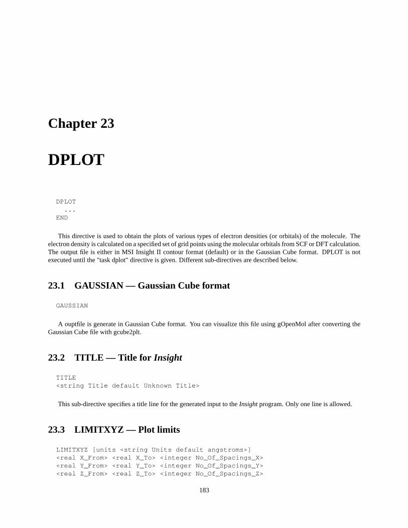
Chapter 23
DPLOT
DPLOT...
END
This directive is used to obtain the plots of various types of electron densities (or orbitals) of the molecule. Theelectron density is calculated on a specified set of grid points using the molecular orbitals from SCF or DFT calculation.The output file is either in MSI Insight II contour format (default) or in the Gaussian Cube format. DPLOT is notexecuted until the "task dplot" directive is given. Different sub-directives are described below.
23.1 GAUSSIAN — Gaussian Cube format
GAUSSIAN
A ouptfile is generate in Gaussian Cube format. You can visualize this file using gOpenMol after converting theGaussian Cube file with gcube2plt.
23.2 TITLE — Title for Insight
TITLE<string Title default Unknown Title>
This sub-directive specifies a title line for the generated input to theInsightprogram. Only one line is allowed.
23.3 LIMITXYZ — Plot limits
LIMITXYZ [units <string Units default angstroms>]<real X_From> <real X_To> <integer No_Of_Spacings_X><real Y_From> <real Y_To> <integer No_Of_Spacings_Y><real Z_From> <real Z_To> <integer No_Of_Spacings_Z>
183
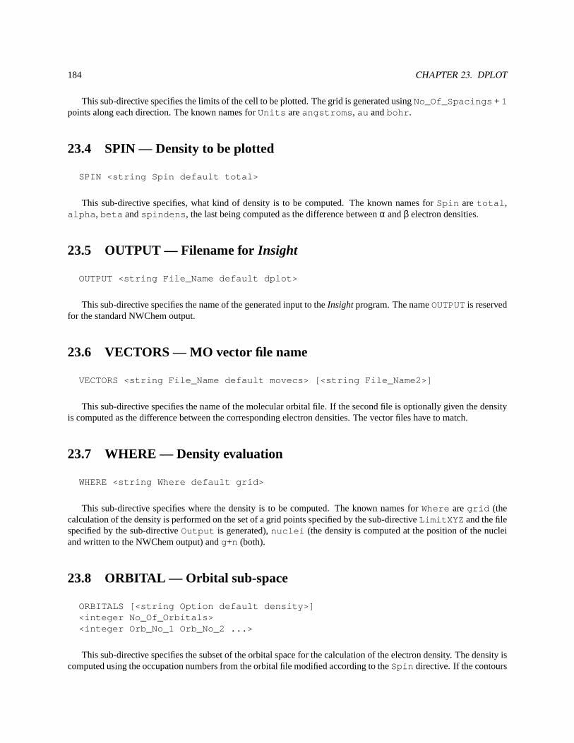
184 CHAPTER 23. DPLOT
This sub-directive specifies the limits of the cell to be plotted. The grid is generated usingNo_Of_Spacings + 1points along each direction. The known names forUnits areangstroms , au andbohr .
23.4 SPIN — Density to be plotted
SPIN <string Spin default total>
This sub-directive specifies, what kind of density is to be computed. The known names forSpin are total ,alpha , beta andspindens , the last being computed as the difference betweenα andβ electron densities.
23.5 OUTPUT — Filename forInsight
OUTPUT <string File_Name default dplot>
This sub-directive specifies the name of the generated input to theInsightprogram. The nameOUTPUTis reservedfor the standard NWChem output.
23.6 VECTORS — MO vector file name
VECTORS <string File_Name default movecs> [<string File_Name2>]
This sub-directive specifies the name of the molecular orbital file. If the second file is optionally given the densityis computed as the difference between the corresponding electron densities. The vector files have to match.
23.7 WHERE — Density evaluation
WHERE <string Where default grid>
This sub-directive specifies where the density is to be computed. The known names forWhere aregrid (thecalculation of the density is performed on the set of a grid points specified by the sub-directiveLimitXYZ and the filespecified by the sub-directiveOutput is generated),nuclei (the density is computed at the position of the nucleiand written to the NWChem output) andg+n (both).
23.8 ORBITAL — Orbital sub-space
ORBITALS [<string Option default density>]<integer No_Of_Orbitals><integer Orb_No_1 Orb_No_2 ...>
This sub-directive specifies the subset of the orbital space for the calculation of the electron density. The density iscomputed using the occupation numbers from the orbital file modified according to theSpin directive. If the contours
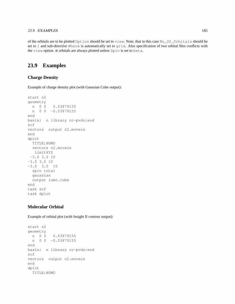
23.9. EXAMPLES 185
of the orbitals are to be plottedOption should be set toview . Note, that in this caseNo_Of_Orbitals should beset to1 and sub-directiveWhere is automatically set togrid . Also specification of two orbital files conflicts withtheview option.α orbitals are always plotted unlessSpin is set tobeta .
23.9 Examples
Charge Density
Example of charge density plot (with Gaussian Cube output):
start n2geometry
n 0 0 0.53879155n 0 0 -0.53879155
endbasis; n library cc-pvdz;endscfvectors output n2.movecsenddplot
TITLE;HOMOvectors n2.movecs
LimitXYZ-3.0 3.0 10
-3.0 3.0 10-3.0 3.0 10
spin totalgaussianoutput lumo.cube
endtask scftask dplot
Molecular Orbital
Example of orbital plot (with Insight II contour output):
start n2geometry
n 0 0 0.53879155n 0 0 -0.53879155
endbasis; n library cc-pvdz;endscfvectors output n2.movecsenddplot
TITLE;HOMO

186 CHAPTER 23. DPLOT
vectors n2.movecsLimitXYZ
-3.0 3.0 10-3.0 3.0 10-3.0 3.0 10
spin totalorbitals view; 1; 7output homo.grd
endtask scftask dplot
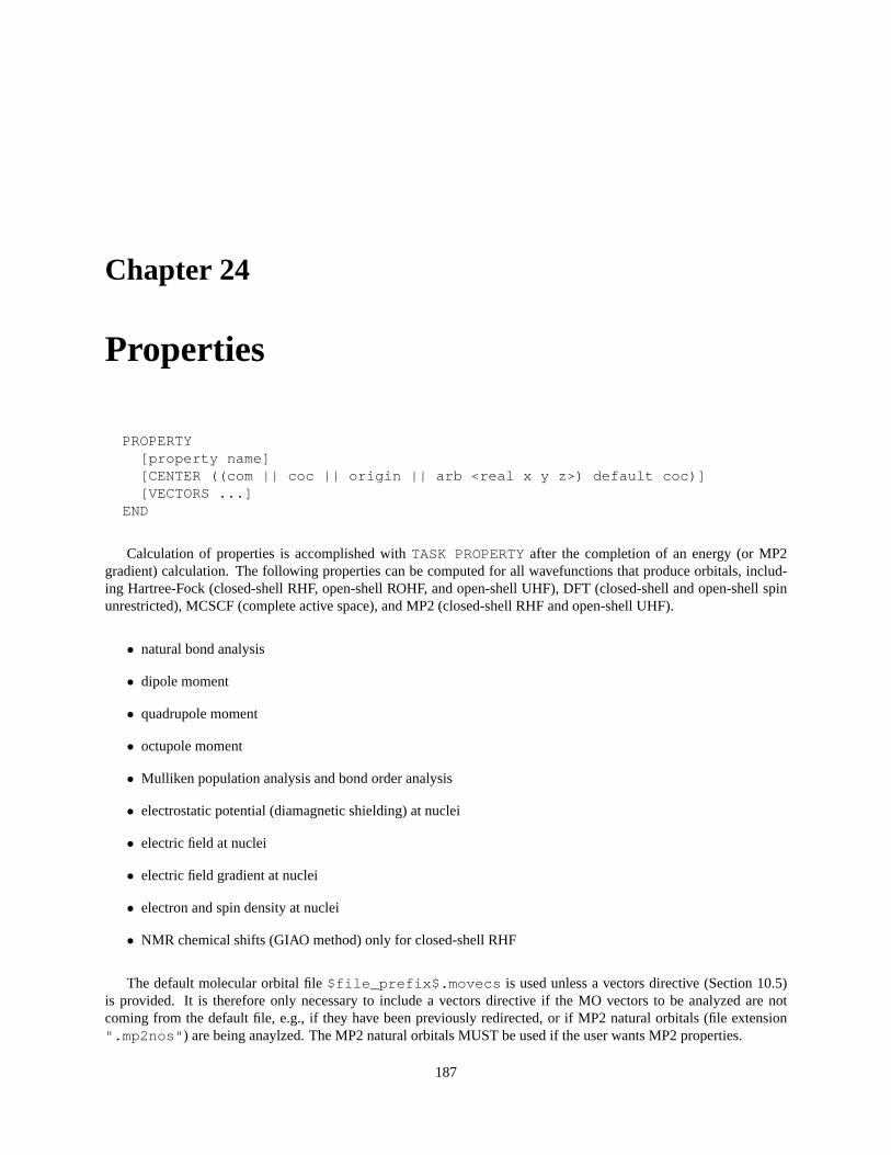
Chapter 24
Properties
PROPERTY[property name][CENTER ((com || coc || origin || arb <real x y z>) default coc)][VECTORS ...]
END
Calculation of properties is accomplished withTASK PROPERTYafter the completion of an energy (or MP2gradient) calculation. The following properties can be computed for all wavefunctions that produce orbitals, includ-ing Hartree-Fock (closed-shell RHF, open-shell ROHF, and open-shell UHF), DFT (closed-shell and open-shell spinunrestricted), MCSCF (complete active space), and MP2 (closed-shell RHF and open-shell UHF).
• natural bond analysis
• dipole moment
• quadrupole moment
• octupole moment
• Mulliken population analysis and bond order analysis
• electrostatic potential (diamagnetic shielding) at nuclei
• electric field at nuclei
• electric field gradient at nuclei
• electron and spin density at nuclei
• NMR chemical shifts (GIAO method) only for closed-shell RHF
The default molecular orbital file$file_prefix$.movecs is used unless a vectors directive (Section 10.5)is provided. It is therefore only necessary to include a vectors directive if the MO vectors to be analyzed are notcoming from the default file, e.g., if they have been previously redirected, or if MP2 natural orbitals (file extension".mp2nos" ) are being anaylzed. The MP2 natural orbitals MUST be used if the user wants MP2 properties.
187
188 CHAPTER 24. PROPERTIES
24.1 Subdirectives
Note that presenting any property input causes all previous property input to be “forgotten”, unlike other NWChemmodules.
Each property can be requested by means of a subdirective among the subdirectives provided :
• nbofile
• dipole
• quadrupole
• octupole
• mulliken
• esp
• efield
• efieldgrad
• electrondensity
• giao
• all
The “all” keyword generates all currently available properties.
The request to NBOFILE does not execute the Natural Bond Analysis code, but simply creates an input file tobe used as input to the stand-alone NBO code. To execute the NBO analysis directly, see Section 33.1. All otherproperties are calculated upon request.
An additional subdirective is provided to specify the origin of the molecular orbitals used in the calculation of themolecular properties. This is the ’vectors’ subdirective, also used in the SCF and DFT tasks. For a full description ofthis subdirective the user is refered to the description found in the SCF description. By default, the input file used forthe calculation of the properties has the .movecs name extension.
The user also has the option to choose the center of expansion for the dipole, quadrupole, and octupole calculations.
[CENTER ((com || coc || origin || arb <real x y z>) default coc)]
com is the center of mass, coc is the center of charge, origin is (0.0, 0.0, 0.0) and arb is any arbitrary point whichmust be accompanied by the coordinated to be used. Currently the x, y, and z coordinates must be given in the sameunits as UNITS in GEOMETRY (See Section 6.1).
24.1.1 Nbofile
Following the successful completion of an electronic structure calculation, a Natural Bond Orbital (NBO) analysismay be carried out in the following way. On restart specify the TASK as PROPERTY and supply the sub-directiveNBOFILE to the PROPERTY directive. NWChem will query the rtdb and construct an ASCII file,<file_prefix>.gen ,that may be used as input to the stand alone version of the NBO program, gennbo.<file_prefix> is equal to stringfollowing the RESTART directive. The input deck may be edited to provide additional options to the NBO calculation,(see the NBO user’s manual for details.) The other option in to directly run the NBO analysis (See Section 33.1 formore information).
Chapter 25
Electrostatic potentials
The NWChem Electrostatic Potential (ESP) module derives partial atomic charges that fit the quantum mechanicalelectrostatic potential on selected grid points.
The ESP module is specified by the NWChem task directive
task esp
The input for the module is taken from the ESP input block
espend
25.1 Grid specification
The grid points for which the quantum mechanical electrostatic potential is evaluated and used in the fitting procedureof the partial atomic charges all lie outside the van der Waals radius of the atoms and within a cutoff distance from theatomic centers. The following input parameters determine the selection of grid points.
• If a grid file is found, the grid will be read from that file. If no grid file is found, or the keyword
recalculate
is given, the grid and the electrostatic potential is recalculated.
• The extent of the grid is determined by
range <real rcut>
wherercut is the maximum distance innmbetween a grid point and any of the atomic centers. When omitted,a default value forrcut of 0.3nm is used.
• The grid spacing is specified by
spacing <real spac>
189
190 CHAPTER 25. ELECTROSTATIC POTENTIALS
wherespac is the grid spacing innm for the regularly spaced grid points. If not specified, a default spacing of0.05nm is used.
• The van der Waals radius of an element can be specified by
radius <integer iatnum> <real atrad>
whereiatnum is the atomic number for which a van der Waals radius ofatrad in nmwill be used in the gridpoint determination. Default values will be used for atoms not specified.
• The probe radius in nm determining the envelope around the molecule is specified by
probe <real probe default 0.07>
• The distance between atomic center and probe center can be multiplied by a constant factor specified by
factor <real factor default 1.0>
All grid points are discarded that lie within a distancefactor*(radius(i)+probe) from any atomi.
• Schwarz screening is applied using
screen [<real scrtol default 1.0D-5>]
25.2 Constraints
Additional constraints to the partial atomic charges can be imposed during the fitting procedure.
• The net charge of a subset of atoms can be constrained using
constrain <real charge> {<integer iatom>}
wherecharge is the net charge of the set of atoms{iatom} . A negative atom numberiatom can be used tospecify that the partial charge of that atom is substracted in the sum for the set.
• The net charge of a sequence of atoms can be constrained using
constrain <real charge> <integer iatom> through <integer jatom>
wherecharge is the net charge of the set of atoms{[iatom:jatom]} .
• A group of atoms can be constrained to have the same charge with
constrain equal {<integer iatom>}
• The individual charge of a group of atoms can be constrained to be equal to those of a second group of atomswith
constrain group <integer iatom> <integer jatom> to <integer katom> <integer latom>
resulting in the same charge for atomsiatom andkatom , for atomsiatom+1 andkatom+1 , ... for atomsjatom andlatom .
25.3. RESTRAINTS 191
• A special constraint
constrain xhn <integer iatom> {<integer jatom>}
can be used to constrain the set{iatom,{jatom}} to zero charge, and constrain all atoms in{jatom} tohave the same charge. This can be used, for example, to restrain a methyl group to zero charge, and have allhydrogen carrying identical charges.
25.3 Restraints
Restraints can be applied to each partial charge using the RESP charge fitting procedure.
• The directive for charge restraining is
restrain [hfree] (harmonic [<real scale>] | \hyperbolic [<real scale> [<real tight>]] \
[maxiter <integer maxit>] [tolerance <real toler>])
wherehfree can be specified to exclude hydrogen atoms from the restaining procecure. Variablescale isthe strength of the restraint potential, with a default of 0.005au for the harmonic restraint and a default valueof 0.001au for the hyperbolic restraint. For the hyperbolic restraints the tightnesstight can be specified tochange the default value of 0.1e. The iteration count that needs to be carried out for the hyperbolic restraintis determined by the maximum number of allowed iterationsmaxiter , with a default value of 25, and thetolerance in the convergence of the partial chargestoler , with a default of 0.001e.

192 CHAPTER 25. ELECTROSTATIC POTENTIALS
Chapter 26
Prepare
Theprepare module is used to set up the necessary files for a molecular dynamics simulation withNWChem. Usersupplied coordinates can be used to generate topology and restart files. The topology file contains all static informationabout a molecular system, such as lists of atoms, bonded interactions and force field parameters. The restart filecontains all dynamic information about a molecular system, such as coordinates, velocities and properties.
Without any input, the prepare module checks the existence of a topology and restart file for the molecular systems.If these files exist, the module returns to the main task level without action. The module will generate these files whenthey do not exist. Without any input to the module, the generated system will be for a non-solvated isolated solutesystem.
To update existing files, including solvation, the module requires input directives read from an input deck,
prepare...
end
The prepare module performs three sub-tasks:
* sequence generationThis sub-task analyzes the supplied coordinates from a PDB-formatted file or from the input geometry, andgenerates a sequence file, containing the description of the system in terms of basic building blocks found asfragment or segment files in the database directories for the force field used. If these files do not exist, theyare generated based on the supplied coordinates. This process constists of generating a fragment file with thelist of atoms with their force field dependent atom types, partial atomic charges calculated from a Hartree Fockcalculation for the fragment, followed by a restrained electrostatic potential fit, and a connectivity list. Fromthe information on this fragment file the lists of all bonded interactions are generated, and the complete lists arewritten to a segment file.
* topology generationBased on the generated or user-supplied sequence file and the force field specific segment database files, thissub-task compiles the lists of atoms, bonded interactions, excluded pairs, and substitutes the force field param-eters. Special commands may be given to specify interaction parameters that will be changing in a free energyevaluation.
* restart generationUsing the user supplied coordinates and the topology file for the chemical system, this sub-task generates a
193
194 CHAPTER 26. PREPARE
restart file for the system with coordinates, velocities and other dynamic information. This step may includesolvation of the chemical system and specifying periodic boundary conditions.
Files involved in the preparation phase exist in the following hierarchy:
* standardsThe standard database files contain the original force field information. These files are to reside in a directorythat is specified in the file $HOME/.nwchemrc. There will be such a directory for each supported force field.These directories contain fragment files (with extension frg), segment files (with extension sgm) and a parameterfile (with the name of the force field and with extension par).
* extensionsThese database files contain generally accepted extensions to the original force field and are to reside in aseparate directory that is specified in the file $HOME/.nwchemrc. There will be such a directory for eachsupported force field. These directories contain fragment files (with extension frg), segment files (with extensionsgm) and a parameter file (with the name of the force field and with extension par).
* user preferencesThese database files contain user preferred extensions to the original force field and are to reside in a separatedirectory that is specified in the file $HOME/.nwchemrc. Separate directories of this type should be definedfor each supported force field. These directories may contain fragment files (with extension frg), segment files(with extension sgm) and a parameter file (with the name of the force field and with extension par).
* temporary filesTemporary database files contain user preferred extensions to the original force field and are to reside in aseparate directory that is specified in the file $HOME/.nwchemrc. There be such a directory for each supportedforce field. These directories may contain fragment files (with extension frg), segment files (with extension sgm)and a parameter file (with the name of the force field and with extension par). If not specified, temporary fileswill be taken from the current directory.
Data is taken from the database files searched in the above order. If data is specified more than once, the last foundvalues are used. For example, if some standard segment is redefined in a temporary file, the latter one will be used.This allows the user to redefine standards or extensions without having to modify those database files, which mayreside in a generally available, non-modifyable directory.
The most common problems with theprepare module are
The format of the pdb file does not conform to the pdb standard. In particular, atom names need to correspondwith definitions in the fragment and segment database files, and should adhere to IUPAC recommendations asadopted by the pdb standard. If this problem occurs, the pdb file will need to be corrected.
Non-standard segments may contain atoms that could not be atom typed with the existing typing rules in theforce field parameter files. When this happens, additional typing rules can be included in the parameter file, orthe fragment file may be manually typed.
Parameters for atom types or bonded interactions do not exist in the force field. When this happens, additionalparameters may be defined in the parameter files, or the segment file may be edited to include explicit parameters.
26.1 Default database directories
The file $HOME/.nwchemrc may contain the following entries that determine which files are used by the preparemodule.
26.2. SYSTEM NAME AND COORDINATE SOURCE 195
ffield <string ffname>
This entry specifies the default force field. Database files supplied withNWChem currently support values forffname of amber, referring to AMBER95, andcharmm, referring to the academic CHARMM22 force field.
<string ffname>_(s | x | u | t) <string ffdir>
Entries of this type specify the directoryffdir in which force field database files can be found. The preparemodule will only use files in directories specified here. One exception is that files in the current work directory will beused if no directory with temporary files is specified.
<string solvnam> <string solvfil>
This entry may be used to identify a pure solvent restart filesolvfil by a namesolvnam
An example file $HOME/.nwchemrc is:
ffield amberamber_s /msrc/proj/nwchem/share/amber/amber_s/amber_x /msrc/proj/nwchem/share/amber/amber_x/amber_u /usr/people/d3j191/data/amber/amber_u/spce /msrc/proj/nwchem/share/solvents/spce.rstcharmm_s /msrc/proj/nwchem/share/charmm/charmm_s/charmm_x /msrc/proj/nwchem/share/charmm/charmm_x/
26.2 System name and coordinate source
system <string sys_calc>
The system name can be explicitly specified for theprepare module. If not specified, the system name will betaken from a specification in a previousmd input block, or derived from the run time database name.
source ( pdb | rtdb )
The source of the coordinates can be explicitly specified to be from a PDB formatted filecalc .pdb, or from ageometry object in the run time database. If not specified, a pdb file will be used when it exists in the current directoryor the rtdb geometry otherwise.
model <integer modpdb default 0>
If a PDB formatted source file contains different MODELs, themodel keyword can be used to specify whichMODEL will be used to generate the topology and restart file. If not specified, the first MODEL found on the PDBfile will be read.
altloc <character locpdb default ’ ’>
Thealtloc keyword may be used to specify the use of alternate location coordinates on a PDB file.
196 CHAPTER 26. PREPARE
chain <character chnpdb default ’ ’>
Thechain keyword may be used to specify the chain identifier for coordinates on a PDB file.
sscyx
Keywordsscyx may be used to rename cysteine residues that form sulphur bridges to CYX.
hbuild
Keywordhbuild may be used to add hydrogen atoms to the unknown segments of the structure found on the pdbfile.
26.3 Sequence file generation
If no existing sequence file is present in the current directory, or if thenew_seq keyword was specified in theprepareinput deck, a new sequence file is generated from information from the pdb file, and the following input directives.
maxscf <integer maxscf default 20>
Variable maxscf specifies the maximum number of atoms in a segment for which partial atomic charges will bedetermined from an SCF calculation followed by RESP charge fitting. For larger segments a crude partial chargeguestimation will be done.
qscale <real qscale default 1.0>
Variable qscale specifies the factor with which SCF/RESP determined charges will be multiplied.
modify sequence { <integer sgmnum>:<string sgmnam> }
This command specifies that segmentsgmnamshould be used for segment with numbersgmnum. This commandcan be used to specify a particular protonation state. For example, the following command specifies that residue 114is a hystidine protonated at the Nε site and residue 202 is a hystidine protonated at the Nδ site:
modify sequence 114:HIE 202:HID
Links between atoms can be enforced with
link <string atomname> <string atomname>
For example, to link atom SG in segment 20 with atom FE in segment 55, use:
link 20:_SG 55:FE
26.4. TOPOLOGY FILE GENERATION 197
The format of the sequence file is given in Table 30.8. In addition to the list of segments this file also includeslinks between non-standard segments or other non-standard links. These links are generated based on distances foundbetween atoms on the pdb file. When atoms are involved in such non-standard links that have not been identified inthe fragment of segment files as a non-chain link atom, the prepare module will ignore these links and report them asskipped. If one or more of these links are required, the user has to include them with explicit link directives in thesequence file, making them forced links. Alternatively, these links can be made forced-links by changinglink intoLINK in the sequence file.
fraction { <integer imol> }
Directivefraction can be used to separate solute molecules into fractions for which energies will be separatelyreported during molecular dynamics simulations. The listed molecules will be the last molecule in a fraction. Up to10 molecules may be specified in this directive.
counter <integer num> <string ion>
Directivecounter addsnumcounter ions of typeion to the sequence file. Up to 10counter directives mayappear in the input block.
26.4 Topology file generation
new_top [ new_seq ]
Keywordnew_top is used to force the generation of a new topology file. An existing topology file for the systemin the current directory will be overwritten. If keywordnew_seq is also specified, an existing sequence file will alsobe overwritten with a newly generated file.
amber | charmm
The prepare module generates force field specific fragment, segment and topology files. The force field may beexplicitly specified in the prepare input block by specifying its name. CurrentlyAMBER andCHARMM are thesupported force fields. A default force field may be specified in the file $HOME/.nwchemrc.
standard <string dir_s>extensions <string dir_x>user <string dir_u>temporary <string dir_t>
The user can explicitly specify the directories where force field specific databases can be found. These includeforce field standards, extensions, user preferences and temporary database files.Defaults for the directories where database files reside may be specified in the file $HOME/.nwchemrc for each ofthe supported force fields. Fragment, segment and sequence files generated by theprepare module are written in thetemporary directory. When not specified, the current directory will be used. Topology and restart files are alwayscreated in the current directory.
The following directives control the modifications of a topology file. These directives are executed in the orderin which they appear in theprepare input deck. The topology modifying commands are not stored on the run-timedatabase and are, therefor, not persistent.
198 CHAPTER 26. PREPARE
modify atom <string atomname> [set <integer mset> | initial | final] \( type <string atomtyp> | charge <real atomcharge> | \
polar <real atompolar> | dummy | self | quantum )
Thesemodify commands change the atom type, partial atomic charge, atomic polarizability, specify a dummy,self-interaction and quantum atom, respectively. Ifmset is specified, the modification will only apply to the specifiedset, which has to be 1, 2 or 3. If not specified, the modification will be applied to all three sets. Theatomnam shouldbe specified as<integer isgm>:<string name> , whereisgm is the segment number, andname is the atomname. A leading blank in an atom name should be substituted with an underscore. The modify commands may becombined. For example, the following directive changes for the specified atom the charge and atom type in set 2 andspecifies the atom to be a dummy in set 3.
modify atom 12:_C1 set 2 charge 0.12 type CA set 3 dummy
With the following directives modifications can be made for entire segments.
modify segment <integer isgm> [set <integer mset> | initial | final] \( dummy | self | quantum )
Modifications to bonded interaction parameters can be made with the following modify commands.
modify ( bond <string atomtyp> <string atomtyp> | \angle <string atomtyp> <string atomtyp> <string atomtyp> | \
torsion <string atomtyp> <string atomtyp> <string atomtyp> \<string atomtyp> [ multiplicity <integer multip> ] | \plane <string atomtyp> <string atomtyp> <string atomtyp> \<string atomtyp> ) [set <integer mset> | initial | final] \<real value> <real forcon>
whereatomtyp andmset are defined as above,multip is the torsion ultiplicity for which the modification isto be applied,value is the reference bond, angle, torsion angle of out-of-plane angle value respectively, andforconis the force constant for bond, angle, torsion angle of out-of-plane angle. Whenmultip or mset are not defined themodification will be applied to all multiplicities and sets, respectively, for the identified bonded interaction.
After modifying atoms to quantum atoms the bonded interactions in which only quantum atoms are involved areremoved from the bonded lists using
update lists
Error messages resulting from parameters not being defined for bonded interaction in which only quantum atomsare involved are ignored using
ignore
26.5 Appending to an existing topology file
noe <string atom1> <string atom3> \<real dist1> <real dist2> <real dist3> <real forc1> <real forc2>
26.6. GENERATING A RESTART FILE 199
This directive specifies a distance restraint potential between atomsatom1 andatom2, with a harmonic functionwith force constantf orc1 betweendist1 anddist2, and a harmonic function with force constantf orc2 betweendist2anddist3. For distances shorter thandist1 or larger thandist3, a constant force is applied such that force and energyare continuous atdist1 anddist3, respectively. Distances are given in nm, force constants in kJ mol−1 nm−2.
select <integer isel> { <string atom1> }
Directiveselect specifies a group of atoms used in the definition of potential of mean force potentials.
pmf ( zalign | xyplane ) <integer isel> <real forcon1> <real forcon2>pmf distance <integer isel> <integer jsel> \
<real dist1> <real dist2> <real forcon1> <real forcon2>pmf angle <integer isel> <integer jsel> <integer ksel> \
<real angle1> <real angle2> <real forcon1> <real forcon2>pmf torsion <integer isel> <integer jsel> <integer ksel> <integer lsel> \
<real angle1> <real angle2> <real forcon1> <real forcon2>
Directive pmf specifies a potential of mean force potential in terms of the specified atom selection. Optionzalign specifies the atoms in the selection to be restrained to a line parallel to the z-axis. Optionxyplane specifiesthe atoms in the selection to be restrained to a plane perpendicular to the z-axis. Optionsdistance , angle andtorsion , are defined in terms of the center of geometry of the specified atom selections.
26.6 Generating a restart file
new_rst
Keywordnew_rst will cause an existing restart file to be overwritten with a new file.
The follwing directives control the manipulation of restart files, and are executed in the order in which they appearin theprepare input deck.
solvent name <string*3 slvnam default ‘‘HOH’’> \model <string slvmdl default ‘‘spce’’>
The solvent keyword can be used to specify the three letter solvent name as expected on the PDB formatted file,and the name of the solvent model for which solvent coordinates will be used.
solvate [ < real rshell default 1.2 > ] \( [ cube <real edge> ] | \
[ box <real xedge> [ <real xedge> [ <real xedge> ]]] | \[ sphere <real radius> ] |[ troct <real edge> ])
Solvation can be specified to be in a cubic box with specified edge, rectangular box with specified edges, or ina sphere with specified radius. Solvation in a cube or rectangular box will automatically also set periodic boundaryconditions. Solvation in a sphere will only allow simulations without periodic boundary conditions. The size of thecubic and rectangular boxes will be expanded by a length specified by the expand variable. If no shape is specified,solvation will be done for a cubic box with an edge that leaves rshell nm between any solute atom and a periodic imageof any solute atom after the solute has been centered. An explicitwrite is not needed to write the restart file. Thesolvate will write out a filesys_calc .rst.
200 CHAPTER 26. PREPARE
touch <real touch default 0.23>
The variabletouch specifies the minimum distance between a solvent and solute atom for which a solventmolecule will be accepted for solvation.
expand <real xpndw default 0.1>
The variablexpndw specifies the size in nm with which the simulation volume will be increased after solvation.
read [rst | rst_old | pdb] <string filename>write [rst | [solute [<integer nsolvent>]] (pdb | xyz)] <string filename>
These directives read and write the filefilename in the specified format. Thesolute option instructs to writeout the coordinates for solute and all, or if specified the firstnsolvent , crystal solvent molecules only. If no formatis specified, it will be derived from the extension of the filename. Recognized extensions are rst, rst_old (read only),pdb, xyz (write only) and pov (write only). Reading and then writing the same restart file will cause the sub-block sizeinformation to be lost. If this information needs to be retained a shell copy command needs to be used.
scale <real scale default -1.0>
This directive scales the volume and coordinates written to povray files. A negative value of scale (default) scalesthe coordinates to lie in [-1:1].
cpk [<real cpk default 1.0>]
This directive causes povray files to contain cpk model output. The optional value is used to scale the atomic radii.A neagtive value of cpk resets the rendering to stick.
center | centerx | centery | centerz
These directives center the solute center of geometry at the origin, in the y-z plane, in the x-z plane or in the x-yplane, respectively.
orient
This directive orients the solute principal axes.
translate [atom | segment | molecule] \<integer itran> <integer itran> <real xtran(3)>
This directive translates solute atoms in the indicated range by xtran, without checking for bad contacts in theresulting structure.
remove solvent [inside | outside] [x <real xmin> <real xmax>] \[y <real ymin> <real ymax>] [z <real zmin> <real zmax>]
This directive removes solvent molecules inside or outside the specified coordinate range.
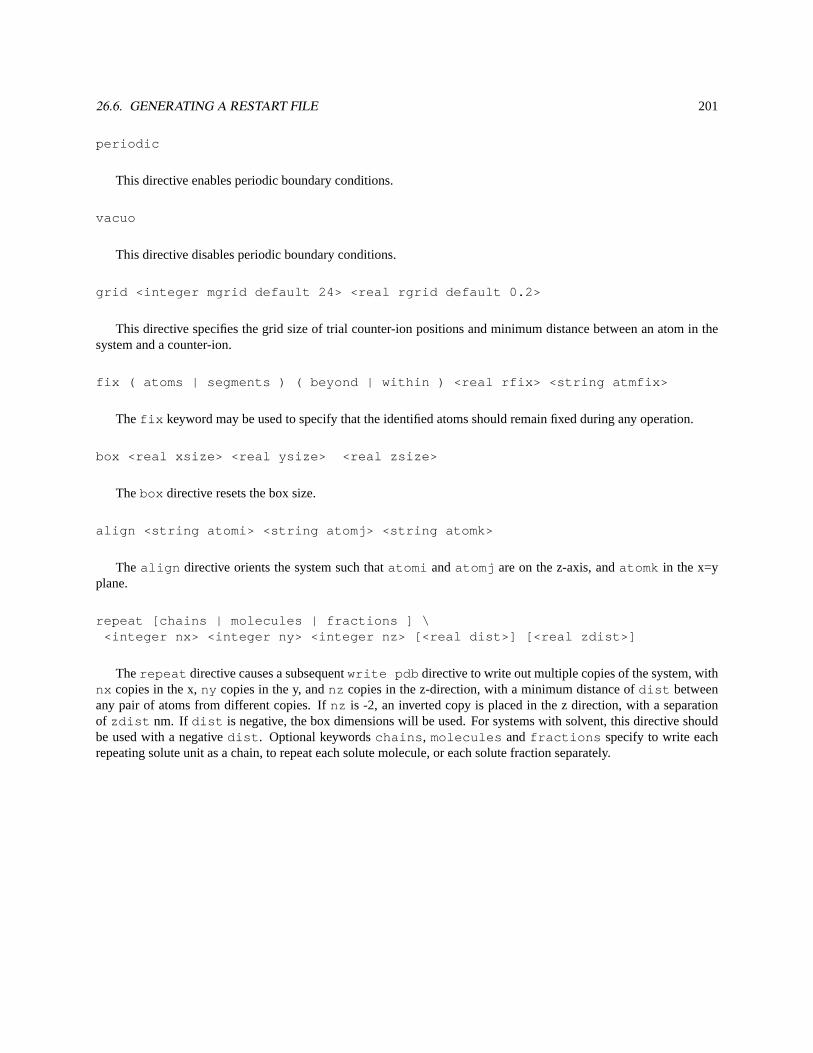
26.6. GENERATING A RESTART FILE 201
periodic
This directive enables periodic boundary conditions.
vacuo
This directive disables periodic boundary conditions.
grid <integer mgrid default 24> <real rgrid default 0.2>
This directive specifies the grid size of trial counter-ion positions and minimum distance between an atom in thesystem and a counter-ion.
fix ( atoms | segments ) ( beyond | within ) <real rfix> <string atmfix>
Thefix keyword may be used to specify that the identified atoms should remain fixed during any operation.
box <real xsize> <real ysize> <real zsize>
Thebox directive resets the box size.
align <string atomi> <string atomj> <string atomk>
The align directive orients the system such thatatomi andatomj are on the z-axis, andatomk in the x=yplane.
repeat [chains | molecules | fractions ] \<integer nx> <integer ny> <integer nz> [<real dist>] [<real zdist>]
Therepeat directive causes a subsequentwrite pdb directive to write out multiple copies of the system, withnx copies in the x,ny copies in the y, andnz copies in the z-direction, with a minimum distance ofdist betweenany pair of atoms from different copies. Ifnz is -2, an inverted copy is placed in the z direction, with a separationof zdist nm. If dist is negative, the box dimensions will be used. For systems with solvent, this directive shouldbe used with a negativedist . Optional keywordschains , molecules and fractions specify to write eachrepeating solute unit as a chain, to repeat each solute molecule, or each solute fraction separately.

202 CHAPTER 26. PREPARE
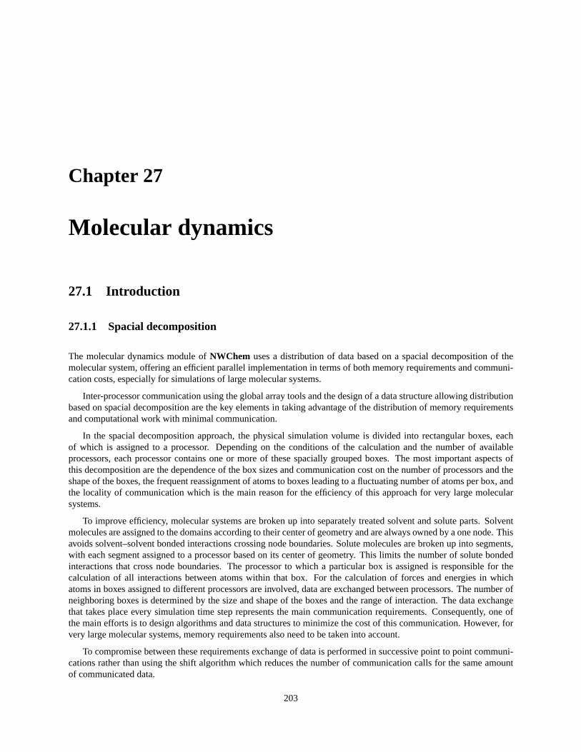
Chapter 27
Molecular dynamics
27.1 Introduction
27.1.1 Spacial decomposition
The molecular dynamics module ofNWChem uses a distribution of data based on a spacial decomposition of themolecular system, offering an efficient parallel implementation in terms of both memory requirements and communi-cation costs, especially for simulations of large molecular systems.
Inter-processor communication using the global array tools and the design of a data structure allowing distributionbased on spacial decomposition are the key elements in taking advantage of the distribution of memory requirementsand computational work with minimal communication.
In the spacial decomposition approach, the physical simulation volume is divided into rectangular boxes, eachof which is assigned to a processor. Depending on the conditions of the calculation and the number of availableprocessors, each processor contains one or more of these spacially grouped boxes. The most important aspects ofthis decomposition are the dependence of the box sizes and communication cost on the number of processors and theshape of the boxes, the frequent reassignment of atoms to boxes leading to a fluctuating number of atoms per box, andthe locality of communication which is the main reason for the efficiency of this approach for very large molecularsystems.
To improve efficiency, molecular systems are broken up into separately treated solvent and solute parts. Solventmolecules are assigned to the domains according to their center of geometry and are always owned by a one node. Thisavoids solvent–solvent bonded interactions crossing node boundaries. Solute molecules are broken up into segments,with each segment assigned to a processor based on its center of geometry. This limits the number of solute bondedinteractions that cross node boundaries. The processor to which a particular box is assigned is responsible for thecalculation of all interactions between atoms within that box. For the calculation of forces and energies in whichatoms in boxes assigned to different processors are involved, data are exchanged between processors. The number ofneighboring boxes is determined by the size and shape of the boxes and the range of interaction. The data exchangethat takes place every simulation time step represents the main communication requirements. Consequently, one ofthe main efforts is to design algorithms and data structures to minimize the cost of this communication. However, forvery large molecular systems, memory requirements also need to be taken into account.
To compromise between these requirements exchange of data is performed in successive point to point communi-cations rather than using the shift algorithm which reduces the number of communication calls for the same amountof communicated data.
203
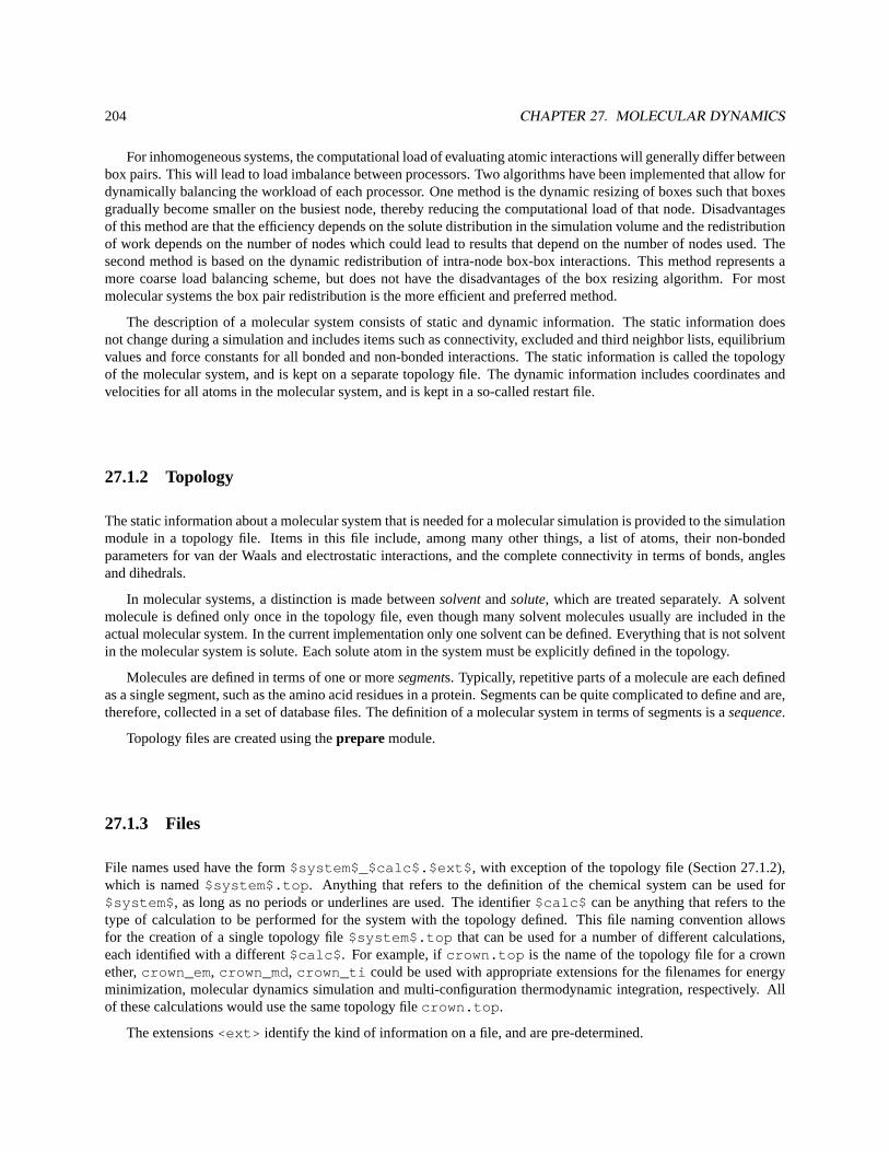
204 CHAPTER 27. MOLECULAR DYNAMICS
For inhomogeneous systems, the computational load of evaluating atomic interactions will generally differ betweenbox pairs. This will lead to load imbalance between processors. Two algorithms have been implemented that allow fordynamically balancing the workload of each processor. One method is the dynamic resizing of boxes such that boxesgradually become smaller on the busiest node, thereby reducing the computational load of that node. Disadvantagesof this method are that the efficiency depends on the solute distribution in the simulation volume and the redistributionof work depends on the number of nodes which could lead to results that depend on the number of nodes used. Thesecond method is based on the dynamic redistribution of intra-node box-box interactions. This method represents amore coarse load balancing scheme, but does not have the disadvantages of the box resizing algorithm. For mostmolecular systems the box pair redistribution is the more efficient and preferred method.
The description of a molecular system consists of static and dynamic information. The static information doesnot change during a simulation and includes items such as connectivity, excluded and third neighbor lists, equilibriumvalues and force constants for all bonded and non-bonded interactions. The static information is called the topologyof the molecular system, and is kept on a separate topology file. The dynamic information includes coordinates andvelocities for all atoms in the molecular system, and is kept in a so-called restart file.
27.1.2 Topology
The static information about a molecular system that is needed for a molecular simulation is provided to the simulationmodule in a topology file. Items in this file include, among many other things, a list of atoms, their non-bondedparameters for van der Waals and electrostatic interactions, and the complete connectivity in terms of bonds, anglesand dihedrals.
In molecular systems, a distinction is made betweensolventandsolute, which are treated separately. A solventmolecule is defined only once in the topology file, even though many solvent molecules usually are included in theactual molecular system. In the current implementation only one solvent can be defined. Everything that is not solventin the molecular system is solute. Each solute atom in the system must be explicitly defined in the topology.
Molecules are defined in terms of one or moresegments. Typically, repetitive parts of a molecule are each definedas a single segment, such as the amino acid residues in a protein. Segments can be quite complicated to define and are,therefore, collected in a set of database files. The definition of a molecular system in terms of segments is asequence.
Topology files are created using theprepare module.
27.1.3 Files
File names used have the form$system$_$calc$.$ext$ , with exception of the topology file (Section 27.1.2),which is named$system$.top . Anything that refers to the definition of the chemical system can be used for$system$ , as long as no periods or underlines are used. The identifier$calc$ can be anything that refers to thetype of calculation to be performed for the system with the topology defined. This file naming convention allowsfor the creation of a single topology file$system$.top that can be used for a number of different calculations,each identified with a different$calc$ . For example, ifcrown.top is the name of the topology file for a crownether,crown_em , crown_md , crown_ti could be used with appropriate extensions for the filenames for energyminimization, molecular dynamics simulation and multi-configuration thermodynamic integration, respectively. Allof these calculations would use the same topology filecrown.top .
The extensions<ext> identify the kind of information on a file, and are pre-determined.
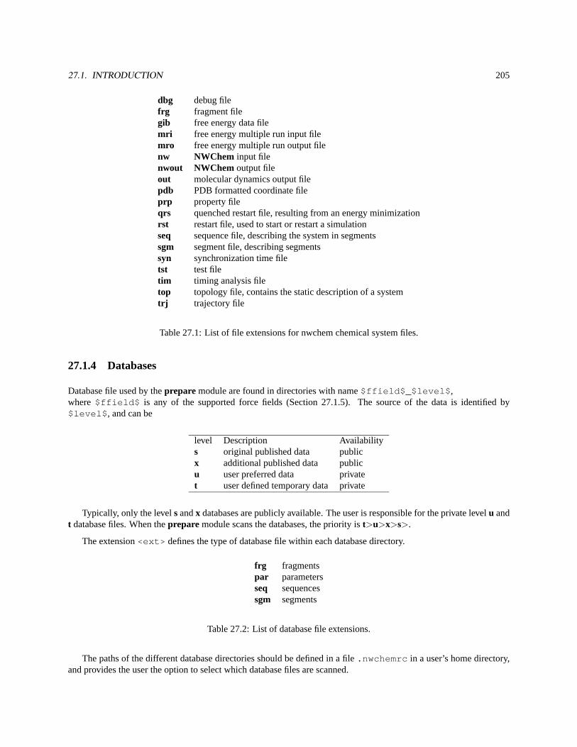
27.1. INTRODUCTION 205
dbg debug filefrg fragment filegib free energy data filemri free energy multiple run input filemro free energy multiple run output filenw NWChem input filenwout NWChem output fileout molecular dynamics output filepdb PDB formatted coordinate fileprp property fileqrs quenched restart file, resulting from an energy minimizationrst restart file, used to start or restart a simulationseq sequence file, describing the system in segmentssgm segment file, describing segmentssyn synchronization time filetst test filetim timing analysis filetop topology file, contains the static description of a systemtrj trajectory file
Table 27.1: List of file extensions for nwchem chemical system files.
27.1.4 Databases
Database file used by theprepare module are found in directories with name$ffield$_$level$ ,where$ffield$ is any of the supported force fields (Section 27.1.5). The source of the data is identified by$level$ , and can be
level Description Availabilitys original published data publicx additional published data publicu user preferred data privatet user defined temporary data private
Typically, only the levelsandx databases are publicly available. The user is responsible for the private levelu andt database files. When theprepare module scans the databases, the priority ist>u>x>s>.
The extension<ext> defines the type of database file within each database directory.
frg fragmentspar parametersseq sequencessgm segments
Table 27.2: List of database file extensions.
The paths of the different database directories should be defined in a file.nwchemrc in a user’s home directory,and provides the user the option to select which database files are scanned.
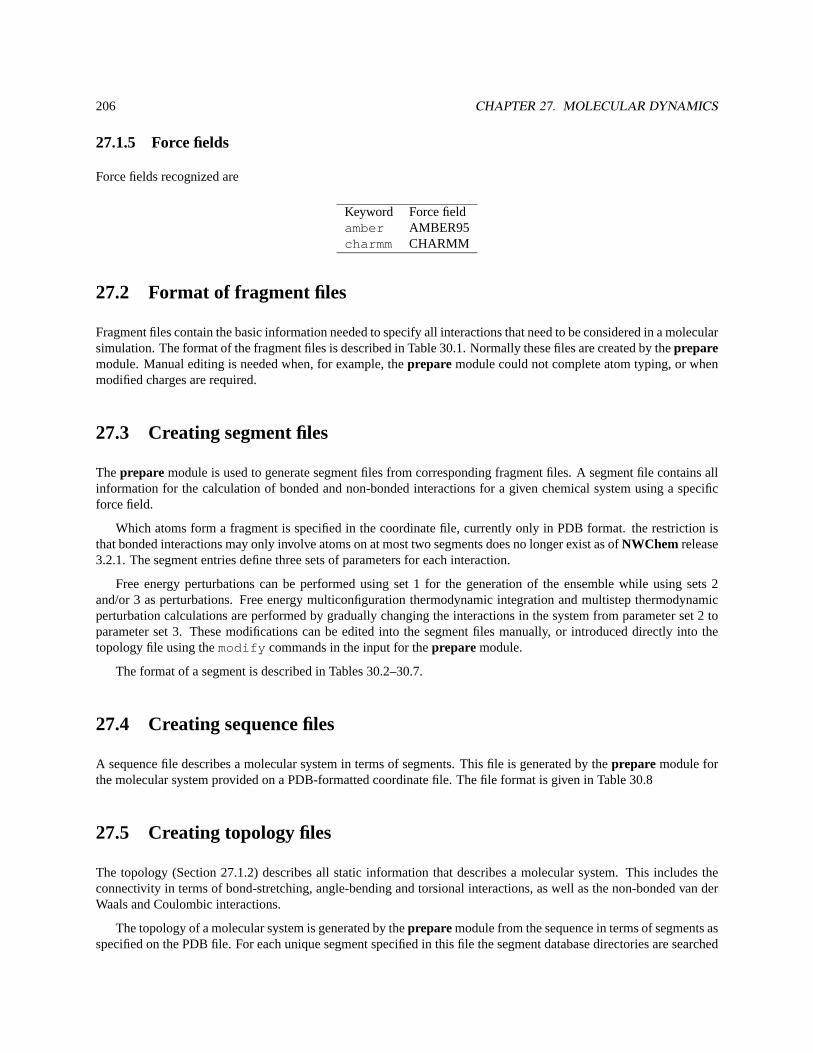
206 CHAPTER 27. MOLECULAR DYNAMICS
27.1.5 Force fields
Force fields recognized are
Keyword Force fieldamber AMBER95charmm CHARMM
27.2 Format of fragment files
Fragment files contain the basic information needed to specify all interactions that need to be considered in a molecularsimulation. The format of the fragment files is described in Table 30.1. Normally these files are created by thepreparemodule. Manual editing is needed when, for example, theprepare module could not complete atom typing, or whenmodified charges are required.
27.3 Creating segment files
Theprepare module is used to generate segment files from corresponding fragment files. A segment file contains allinformation for the calculation of bonded and non-bonded interactions for a given chemical system using a specificforce field.
Which atoms form a fragment is specified in the coordinate file, currently only in PDB format. the restriction isthat bonded interactions may only involve atoms on at most two segments does no longer exist as ofNWChem release3.2.1. The segment entries define three sets of parameters for each interaction.
Free energy perturbations can be performed using set 1 for the generation of the ensemble while using sets 2and/or 3 as perturbations. Free energy multiconfiguration thermodynamic integration and multistep thermodynamicperturbation calculations are performed by gradually changing the interactions in the system from parameter set 2 toparameter set 3. These modifications can be edited into the segment files manually, or introduced directly into thetopology file using themodify commands in the input for theprepare module.
The format of a segment is described in Tables 30.2–30.7.
27.4 Creating sequence files
A sequence file describes a molecular system in terms of segments. This file is generated by theprepare module forthe molecular system provided on a PDB-formatted coordinate file. The file format is given in Table 30.8
27.5 Creating topology files
The topology (Section 27.1.2) describes all static information that describes a molecular system. This includes theconnectivity in terms of bond-stretching, angle-bending and torsional interactions, as well as the non-bonded van derWaals and Coulombic interactions.
The topology of a molecular system is generated by theprepare module from the sequence in terms of segments asspecified on the PDB file. For each unique segment specified in this file the segment database directories are searched
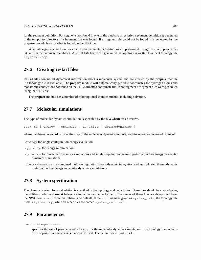
27.6. CREATING RESTART FILES 207
for the segment definition. For segments not found in one of the database directories a segment definition is generatedin the temporary directory if a fragment file was found. If a fragment file could not be found, it is generated by theprepare module base on what is found on the PDB file.
When all segments are found or created, the parameter substitutions are performed, using force field parameterstaken from the parameter databases. After all lists have been generated the topology is written to a local topology file$system$.top .
27.6 Creating restart files
Restart files contain all dynamical information about a molecular system and are created by theprepare moduleif a topology file is available. Theprepare module will automatically generate coordinates for hydrogen atoms andmonatomic counter ions not found on the PDB formatted coordinate file, if no fragment or segment files were generatedusing that PDB file.
Theprepare module has a number of other optional input command, including solvation.
27.7 Molecular simulations
The type of molecular dynamics simulation is specified by theNWChem task directive.
task md [ energy | optimize | dynamics | thermodynamics ]
where the theory keywordmdspecifies use of the molecular dynamics module, and the operation keyword is one of
energy for single configuration energy evaluation
optimize for energy minimization
dynamics for molecular dynamics simulations and single step thermodynamic perturbation free energy moleculardynamics simulations
thermodynamics for combined multi-configuration thermodynamic integration and multiple step thermodynamicperturbation free energy molecular dynamics simulations.
27.8 System specification
The chemical system for a calculation is specified in the topology and restart files. These files should be created usingthe utilitiesnwtop andnwrst before a simulation can be performed. The names of these files are determined fromtheNWChem start directive. There is no default. If thertdb name is given assystem_calc , the topology fileused issystem.top , while all other files are namedsystem_calc.ext .
27.9 Parameter set
set <integer iset>
specifies the use of parameter set<iset> for the molecular dynamics simulation. The topology file containsthree separate parameters sets that can be used. The default for<iset> is 1.
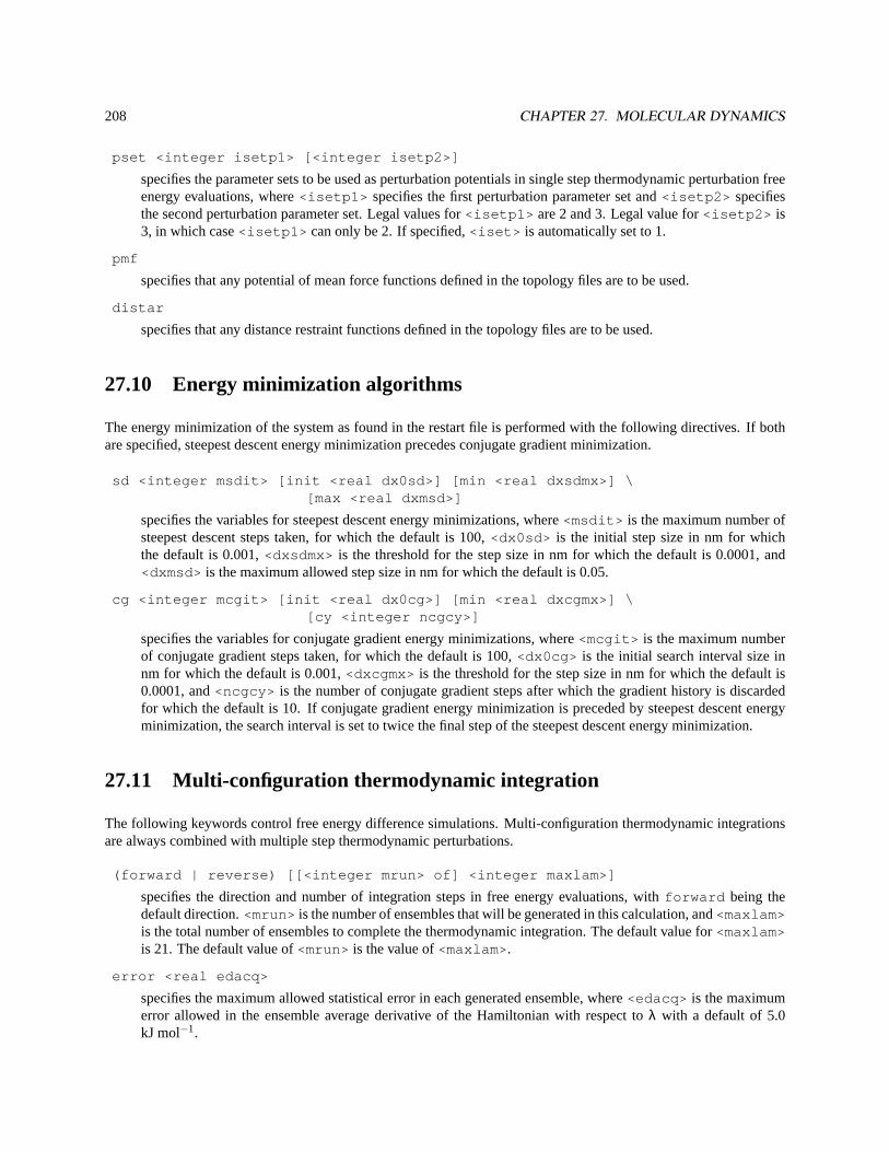
208 CHAPTER 27. MOLECULAR DYNAMICS
pset <integer isetp1> [<integer isetp2>]
specifies the parameter sets to be used as perturbation potentials in single step thermodynamic perturbation freeenergy evaluations, where<isetp1> specifies the first perturbation parameter set and<isetp2> specifiesthe second perturbation parameter set. Legal values for<isetp1> are 2 and 3. Legal value for<isetp2> is3, in which case<isetp1> can only be 2. If specified,<iset> is automatically set to 1.
pmf
specifies that any potential of mean force functions defined in the topology files are to be used.
distar
specifies that any distance restraint functions defined in the topology files are to be used.
27.10 Energy minimization algorithms
The energy minimization of the system as found in the restart file is performed with the following directives. If bothare specified, steepest descent energy minimization precedes conjugate gradient minimization.
sd <integer msdit> [init <real dx0sd>] [min <real dxsdmx>] \[max <real dxmsd>]
specifies the variables for steepest descent energy minimizations, where<msdit> is the maximum number ofsteepest descent steps taken, for which the default is 100,<dx0sd> is the initial step size in nm for whichthe default is 0.001,<dxsdmx> is the threshold for the step size in nm for which the default is 0.0001, and<dxmsd> is the maximum allowed step size in nm for which the default is 0.05.
cg <integer mcgit> [init <real dx0cg>] [min <real dxcgmx>] \[cy <integer ncgcy>]
specifies the variables for conjugate gradient energy minimizations, where<mcgit> is the maximum numberof conjugate gradient steps taken, for which the default is 100,<dx0cg> is the initial search interval size innm for which the default is 0.001,<dxcgmx> is the threshold for the step size in nm for which the default is0.0001, and<ncgcy> is the number of conjugate gradient steps after which the gradient history is discardedfor which the default is 10. If conjugate gradient energy minimization is preceded by steepest descent energyminimization, the search interval is set to twice the final step of the steepest descent energy minimization.
27.11 Multi-configuration thermodynamic integration
The following keywords control free energy difference simulations. Multi-configuration thermodynamic integrationsare always combined with multiple step thermodynamic perturbations.
(forward | reverse) [[<integer mrun> of] <integer maxlam>]
specifies the direction and number of integration steps in free energy evaluations, withforward being thedefault direction.<mrun> is the number of ensembles that will be generated in this calculation, and<maxlam>is the total number of ensembles to complete the thermodynamic integration. The default value for<maxlam>is 21. The default value of<mrun> is the value of<maxlam> .
error <real edacq>
specifies the maximum allowed statistical error in each generated ensemble, where<edacq> is the maximumerror allowed in the ensemble average derivative of the Hamiltonian with respect toλ with a default of 5.0kJ mol−1.
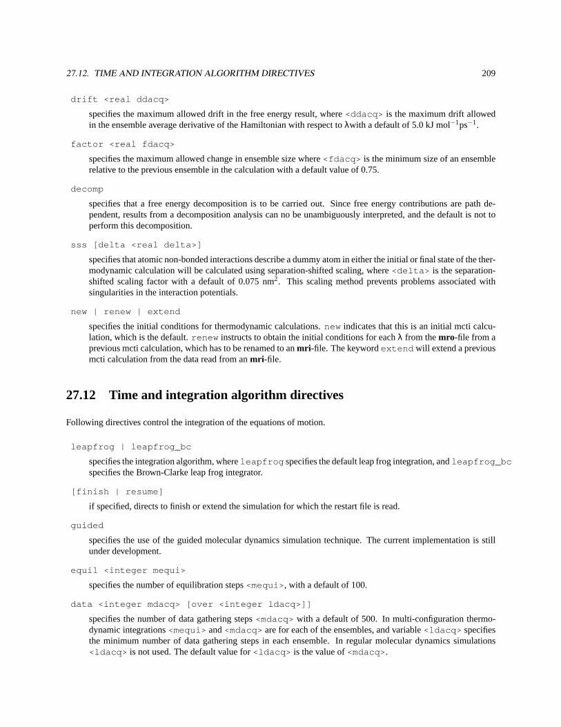
27.12. TIME AND INTEGRATION ALGORITHM DIRECTIVES 209
drift <real ddacq>
specifies the maximum allowed drift in the free energy result, where<ddacq> is the maximum drift allowedin the ensemble average derivative of the Hamiltonian with respect toλwith a default of 5.0 kJ mol−1ps−1.
factor <real fdacq>
specifies the maximum allowed change in ensemble size where<fdacq> is the minimum size of an ensemblerelative to the previous ensemble in the calculation with a default value of 0.75.
decomp
specifies that a free energy decomposition is to be carried out. Since free energy contributions are path de-pendent, results from a decomposition analysis can no be unambiguously interpreted, and the default is not toperform this decomposition.
sss [delta <real delta>]
specifies that atomic non-bonded interactions describe a dummy atom in either the initial or final state of the ther-modynamic calculation will be calculated using separation-shifted scaling, where<delta> is the separation-shifted scaling factor with a default of 0.075 nm2. This scaling method prevents problems associated withsingularities in the interaction potentials.
new | renew | extend
specifies the initial conditions for thermodynamic calculations.new indicates that this is an initial mcti calcu-lation, which is the default.renew instructs to obtain the initial conditions for eachλ from themro-file from aprevious mcti calculation, which has to be renamed to anmri -file. The keywordextend will extend a previousmcti calculation from the data read from anmri -file.
27.12 Time and integration algorithm directives
Following directives control the integration of the equations of motion.
leapfrog | leapfrog_bc
specifies the integration algorithm, whereleapfrog specifies the default leap frog integration, andleapfrog_bcspecifies the Brown-Clarke leap frog integrator.
[finish | resume]
if specified, directs to finish or extend the simulation for which the restart file is read.
guided
specifies the use of the guided molecular dynamics simulation technique. The current implementation is stillunder development.
equil <integer mequi>
specifies the number of equilibration steps<mequi> , with a default of 100.
data <integer mdacq> [over <integer ldacq>]]
specifies the number of data gathering steps<mdacq> with a default of 500. In multi-configuration thermo-dynamic integrations<mequi> and<mdacq> are for each of the ensembles, and variable<ldacq> specifiesthe minimum number of data gathering steps in each ensemble. In regular molecular dynamics simulations<ldacq> is not used. The default value for<ldacq> is the value of<mdacq>.
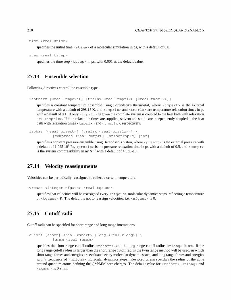
210 CHAPTER 27. MOLECULAR DYNAMICS
time <real stime>
specifies the initial time<stime> of a molecular simulation in ps, with a default of 0.0.
step <real tstep>
specifies the time step<tstep> in ps, with 0.001 as the default value.
27.13 Ensemble selection
Following directives control the ensemble type.
isotherm [<real tmpext>] [trelax <real tmprlx> [<real tmsrlx>]]
specifies a constant temperature ensemble using Berendsen’s thermostat, where<tmpext> is the externaltemperature with a default of 298.15 K, and<tmprlx> and<tmsrlx> are temperature relaxation times in pswith a default of 0.1. If only<tmprlx> is given the complete system is coupled to the heat bath with relaxationtime<tmprlx> . If both relaxation times are supplied, solvent and solute are independently coupled to the heatbath with relaxation times<tmprlx> and<tmsrlx> , respectively.
isobar [<real prsext>] [trelax <real prsrlx> ] \[compress <real compr>] [anisotropic] [noz]
specifies a constant pressure ensemble using Berendsen’s piston, where<prsext> is the external pressure witha default of 1.025 105 Pa,<prsrlx> is the pressure relaxation time in ps with a default of 0.5, and<compr>is the system compressibility in m2N−1 with a default of 4.53E-10.
27.14 Velocity reassignments
Velocities can be periodically reassigned to reflect a certain temperature.
vreass <integer nfgaus> <real tgauss>
specifies that velocities will be reassigned every<nfgaus> molecular dynamics steps, reflecting a temperatureof <tgauss> K. The default is not to reassign velocities, i.e.<nfgaus> is 0.
27.15 Cutoff radii
Cutoff radii can be specified for short range and long range interactions.
cutoff [short] <real rshort> [long <real rlong>] \[qmmm <real rqmmm>]
specifies the short range cutoff radius<rshort> , and the long range cutoff radius<rlong> in nm. If thelong range cutoff radius is larger than the short range cutoff radius the twin range method will be used, in whichshort range forces and energies are evaluated every molecular dynamics step, and long range forces and energieswith a frequency of<nflong> molecular dynamics steps. Keywordqmmmspecifies the radius of the zonearound quantum atoms defining the QM/MM bare charges. The default value for<rshort> , <rlong> and<rqmmm>is 0.9 nm.
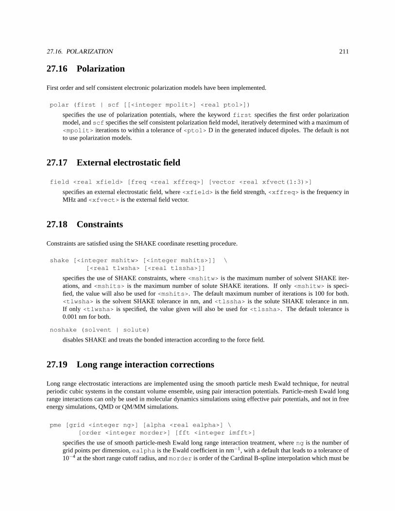
27.16. POLARIZATION 211
27.16 Polarization
First order and self consistent electronic polarization models have been implemented.
polar (first | scf [[<integer mpolit>] <real ptol>])
specifies the use of polarization potentials, where the keywordfirst specifies the first order polarizationmodel, andscf specifies the self consistent polarization field model, iteratively determined with a maximum of<mpolit> iterations to within a tolerance of<ptol> D in the generated induced dipoles. The default is notto use polarization models.
27.17 External electrostatic field
field <real xfield> [freq <real xffreq>] [vector <real xfvect(1:3)>]
specifies an external electrostatic field, where<xfield> is the field strength,<xffreq> is the frequency inMHz and<xfvect> is the external field vector.
27.18 Constraints
Constraints are satisfied using the SHAKE coordinate resetting procedure.
shake [<integer mshitw> [<integer mshits>]] \[<real tlwsha> [<real tlssha>]]
specifies the use of SHAKE constraints, where<mshitw> is the maximum number of solvent SHAKE iter-ations, and<mshits> is the maximum number of solute SHAKE iterations. If only<mshitw> is speci-fied, the value will also be used for<mshits> . The default maximum number of iterations is 100 for both.<tlwsha> is the solvent SHAKE tolerance in nm, and<tlssha> is the solute SHAKE tolerance in nm.If only <tlwsha> is specified, the value given will also be used for<tlssha> . The default tolerance is0.001 nm for both.
noshake (solvent | solute)
disables SHAKE and treats the bonded interaction according to the force field.
27.19 Long range interaction corrections
Long range electrostatic interactions are implemented using the smooth particle mesh Ewald technique, for neutralperiodic cubic systems in the constant volume ensemble, using pair interaction potentials. Particle-mesh Ewald longrange interactions can only be used in molecular dynamics simulations using effective pair potentials, and not in freeenergy simulations, QMD or QM/MM simulations.
pme [grid <integer ng>] [alpha <real ealpha>] \[order <integer morder>] [fft <integer imfft>]
specifies the use of smooth particle-mesh Ewald long range interaction treatment, whereng is the number ofgrid points per dimension,ealpha is the Ewald coefficient in nm−1, with a default that leads to a tolerance of10−4 at the short range cutoff radius, andmorder is order of the Cardinal B-spline interpolation which must be
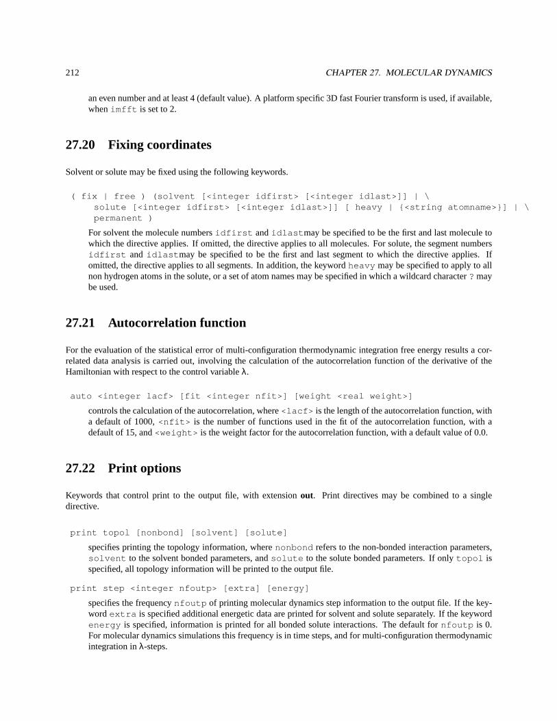
212 CHAPTER 27. MOLECULAR DYNAMICS
an even number and at least 4 (default value). A platform specific 3D fast Fourier transform is used, if available,whenimfft is set to 2.
27.20 Fixing coordinates
Solvent or solute may be fixed using the following keywords.
( fix | free ) (solvent [<integer idfirst> [<integer idlast>]] | \solute [<integer idfirst> [<integer idlast>]] [ heavy | {<string atomname>}] | \permanent )
For solvent the molecule numbersidfirst andidlast may be specified to be the first and last molecule towhich the directive applies. If omitted, the directive applies to all molecules. For solute, the segment numbersidfirst and idlast may be specified to be the first and last segment to which the directive applies. Ifomitted, the directive applies to all segments. In addition, the keywordheavy may be specified to apply to allnon hydrogen atoms in the solute, or a set of atom names may be specified in which a wildcard character? maybe used.
27.21 Autocorrelation function
For the evaluation of the statistical error of multi-configuration thermodynamic integration free energy results a cor-related data analysis is carried out, involving the calculation of the autocorrelation function of the derivative of theHamiltonian with respect to the control variableλ.
auto <integer lacf> [fit <integer nfit>] [weight <real weight>]
controls the calculation of the autocorrelation, where<lacf> is the length of the autocorrelation function, witha default of 1000,<nfit> is the number of functions used in the fit of the autocorrelation function, with adefault of 15, and<weight> is the weight factor for the autocorrelation function, with a default value of 0.0.
27.22 Print options
Keywords that control print to the output file, with extensionout. Print directives may be combined to a singledirective.
print topol [nonbond] [solvent] [solute]
specifies printing the topology information, wherenonbond refers to the non-bonded interaction parameters,solvent to the solvent bonded parameters, andsolute to the solute bonded parameters. If onlytopol isspecified, all topology information will be printed to the output file.
print step <integer nfoutp> [extra] [energy]
specifies the frequencynfoutp of printing molecular dynamics step information to the output file. If the key-word extra is specified additional energetic data are printed for solvent and solute separately. If the keywordenergy is specified, information is printed for all bonded solute interactions. The default fornfoutp is 0.For molecular dynamics simulations this frequency is in time steps, and for multi-configuration thermodynamicintegration inλ-steps.
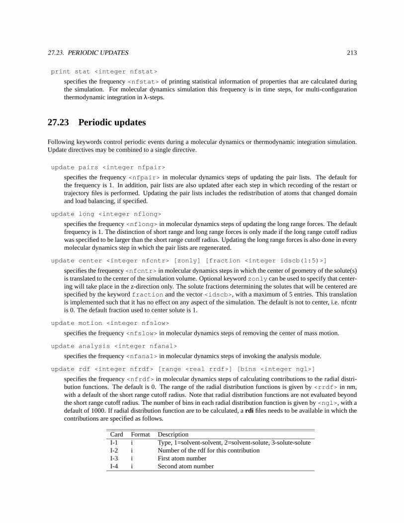
27.23. PERIODIC UPDATES 213
print stat <integer nfstat>
specifies the frequency<nfstat> of printing statistical information of properties that are calculated duringthe simulation. For molecular dynamics simulation this frequency is in time steps, for multi-configurationthermodynamic integration inλ-steps.
27.23 Periodic updates
Following keywords control periodic events during a molecular dynamics or thermodynamic integration simulation.Update directives may be combined to a single directive.
update pairs <integer nfpair>
specifies the frequency<nfpair> in molecular dynamics steps of updating the pair lists. The default forthe frequency is 1. In addition, pair lists are also updated after each step in which recording of the restart ortrajectory files is performed. Updating the pair lists includes the redistribution of atoms that changed domainand load balancing, if specified.
update long <integer nflong>
specifies the frequency<nflong> in molecular dynamics steps of updating the long range forces. The defaultfrequency is 1. The distinction of short range and long range forces is only made if the long range cutoff radiuswas specified to be larger than the short range cutoff radius. Updating the long range forces is also done in everymolecular dynamics step in which the pair lists are regenerated.
update center <integer nfcntr> [zonly] [fraction <integer idscb(1:5)>]
specifies the frequency<nfcntr> in molecular dynamics steps in which the center of geometry of the solute(s)is translated to the center of the simulation volume. Optional keywordzonly can be used to specify that center-ing will take place in the z-direction only. The solute fractions determining the solutes that will be centered arespecified by the keywordfraction and the vector<idscb> , with a maximum of 5 entries. This translationis implemented such that it has no effect on any aspect of the simulation. The default is not to center, i.e. nfcntris 0. The default fraction used to center solute is 1.
update motion <integer nfslow>
specifies the frequency<nfslow> in molecular dynamics steps of removing the center of mass motion.
update analysis <integer nfanal>
specifies the frequency<nfanal> in molecular dynamics steps of invoking the analysis module.
update rdf <integer nfrdf> [range <real rrdf>] [bins <integer ngl>]
specifies the frequency<nfrdf> in molecular dynamics steps of calculating contributions to the radial distri-bution functions. The default is 0. The range of the radial distribution functions is given by<rrdf> in nm,with a default of the short range cutoff radius. Note that radial distribution functions are not evaluated beyondthe short range cutoff radius. The number of bins in each radial distribution function is given by<ngl> , with adefault of 1000. If radial distribution function are to be calculated, ardi files needs to be available in which thecontributions are specified as follows.
Card Format DescriptionI-1 i Type, 1=solvent-solvent, 2=solvent-solute, 3-solute-soluteI-2 i Number of the rdf for this contributionI-3 i First atom numberI-4 i Second atom number

214 CHAPTER 27. MOLECULAR DYNAMICS
27.24 Recording
The following keywords control recording data to file. Record directives may be combined to a single directive.
record rest <integer nfrest> [keep]
specifies the frequency<nfrest> in molecular dynamics steps of rewriting the restart file, with extensionrst . For multi-configuration thermodynamic integration simulations the frequency is in steps inλ. The defaultis not to record. The restart file is used to start or restart simulations. The keywordkeep causes all restart fileswritten to be kept on disk, rather than to be overwritten.
record coord <integer nfcoor>
specifies the frequency<nfcoor> in molecular dynamics steps of writing coordinates to the trajectory file.This directive redefines previousrecord coord , record wcoor and record scoor directives. Thedefault is not to record.
record wcoor <integer nfwcoo>
specifies the frequency<nfcoor> in molecular dynamics steps of writing solvent coordinates to the trajectoryfile. This keyword takes precedent overrecord coord . This directive redefines previousrecord coord ,record wcoor andrecord scoor directives. The default is not to record.
record scoor <integer nfscoo>
specifies the frequency<nfscoo> in molecular dynamics steps of writing solute coordinates to the trajectoryfile. This keyword takes precedent overrecord coord . This directive redefines previousrecord coord ,record wcoor andrecord scoor directives. The default is not to record.
record veloc <integer nfvelo>
specifies the frequency<nfvelo> in molecular dynamics steps of writing velocitiesto the trajectory file. Thisdirective redefines previousrecord veloc , record wvelo andrecord svelo directives. The defaultis not to record.
record wvelo <integer nfwvel>
specifies the frequency<nfvelo> in molecular dynamics steps of writing solvent velocitiesto the trajectoryfile. This keyword takes precedent overrecord veloc . This directive redefines previousrecord veloc ,record wvelo andrecord svelo directives. The default is not to record.
record svelo <integer nfsvel>
specifies the frequency<nfsvel> in molecular dynamics steps of writing solute velocities to the trajectoryfile. This keyword takes precedent overrecord veloc . This directive redefines previousrecord veloc ,record wvelo andrecord svelo directives. The default is not to record.
record prop <integer nfprop>
specifies the frequency<nfprop> in molecular dynamics steps of writing information to the property file, withextensionprp . For multi-configuration thermodynamic integration simulations the frequency is in steps inλ.The default is not to record.
record free <integer nffree>
specifies the frequency<nffree> in multi-configuration thermodynamic integration steps to record data to thefree energy data file, with extensiongib . The default is 1, i.e. to record at everyλ.
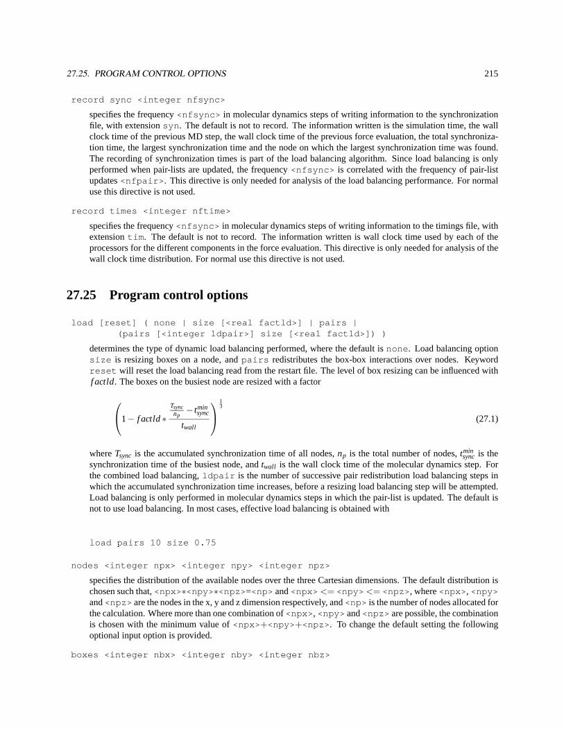
27.25. PROGRAM CONTROL OPTIONS 215
record sync <integer nfsync>
specifies the frequency<nfsync> in molecular dynamics steps of writing information to the synchronizationfile, with extensionsyn . The default is not to record. The information written is the simulation time, the wallclock time of the previous MD step, the wall clock time of the previous force evaluation, the total synchroniza-tion time, the largest synchronization time and the node on which the largest synchronization time was found.The recording of synchronization times is part of the load balancing algorithm. Since load balancing is onlyperformed when pair-lists are updated, the frequency<nfsync> is correlated with the frequency of pair-listupdates<nfpair> . This directive is only needed for analysis of the load balancing performance. For normaluse this directive is not used.
record times <integer nftime>
specifies the frequency<nfsync> in molecular dynamics steps of writing information to the timings file, withextensiontim . The default is not to record. The information written is wall clock time used by each of theprocessors for the different components in the force evaluation. This directive is only needed for analysis of thewall clock time distribution. For normal use this directive is not used.
27.25 Program control options
load [reset] ( none | size [<real factld>] | pairs |(pairs [<integer ldpair>] size [<real factld>]) )
determines the type of dynamic load balancing performed, where the default isnone . Load balancing optionsize is resizing boxes on a node, andpairs redistributes the box-box interactions over nodes. Keywordreset will reset the load balancing read from the restart file. The level of box resizing can be influenced withf actld. The boxes on the busiest node are resized with a factor
1− f actld∗Tsyncnp− tmin
sync
twall
13
(27.1)
whereTsync is the accumulated synchronization time of all nodes,np is the total number of nodes,tminsync is the
synchronization time of the busiest node, andtwall is the wall clock time of the molecular dynamics step. Forthe combined load balancing,ldpair is the number of successive pair redistribution load balancing steps inwhich the accumulated synchronization time increases, before a resizing load balancing step will be attempted.Load balancing is only performed in molecular dynamics steps in which the pair-list is updated. The default isnot to use load balancing. In most cases, effective load balancing is obtained with
load pairs 10 size 0.75
nodes <integer npx> <integer npy> <integer npz>
specifies the distribution of the available nodes over the three Cartesian dimensions. The default distribution ischosen such that,<npx> ∗<npy> ∗<npz> =<np> and<npx> <= <npy> <= <npz> , where<npx> , <npy>and<npz> are the nodes in the x, y and z dimension respectively, and<np> is the number of nodes allocated forthe calculation. Where more than one combination of<npx> , <npy> and<npz> are possible, the combinationis chosen with the minimum value of<npx> +<npy> +<npz> . To change the default setting the followingoptional input option is provided.
boxes <integer nbx> <integer nby> <integer nbz>
216 CHAPTER 27. MOLECULAR DYNAMICS
specifies the distribution of boxes, where<nbx> , <nby> and<nbz> are the number of boxes in x, y and zdirection, respectively. The molecular system is decomposed into boxes that form the smallest unit for com-munication of atomic data between nodes. The size of the boxes is per default set to the short-range cutoffradius. If long-range cutoff radii are used the box size is set to half the long-range cutoff radius if it is largerthan the short-range cutoff. If the number of boxes in a dimension is less than the number of processors in thatdimension, the number of boxes is set to the number of processors.
extra <integer madbox>
sets the number of additional boxes for which memory is allocated. In rare events the amount of memory setaside per node is insufficient to hold all atomic coordinates assigned to that node. This leads to execution whichaborts with the message thatmwmor msa is too small. Jobs may be restarted with additional space allocated bywhere<madbox> is the number of additional boxes that are allocated on each node. The default for<madbox>is 6. In some cases<madbox> can be reduced to 4 if memory usage is a concern. Values of 2 or less will almostcertainly result in memory shortage.
mwm <integer mwmreq>
sets the maximum number of solvent molecules<mwmreq>per node, allowing increased memory to be allo-cated for solvent molecules. This option can be used if execution aborted becausemwmwas too small.
msa <integer msareq>
sets the maximum number of solute atoms<msareq> per node, allowing increased memory to be allocated forsolute atoms. This option can be used if execution aborted becausemsa was too small.
mbb <integer mbbreq>
sets the maximum number of sub-box pairs<mbbreq> per node, allowing increased memory to be allocatedfor the sub-box pair lists. This option can be used if execution aborted becausembbl was too small.
memory <integer memlim>
sets a limit<memlim> in kB on the allocated amount of memory used by the molecular dynamics module. Perdefault all available memory is allocated. Use of this command is required for QM/MM simulations only.
Chapter 28
Analysis
Theanalysismodule is used to analyze molecular trajectories generated by theNWChem molecular dynamics mod-ule, or partial charges generated by theNWChem electrostatic potential fit module. This module should not de run inparallel mode.
Directives for theanalysismodule are read from an input deck,
analysis...
end
The analysis is performed as post-analysis of trajectory files through using the task directive
task analysis
or
task analyze
28.1 Reference coordinates
Most analyses require a set of reference coordinates. These coordinates are read from aNWChem restart file by thedirective,
reference <string filename>
where filename is the name of an existing restart file. This input directive is required.
28.2 File specification
The trajectory file(s) to be analyzed are specified with
217
218 CHAPTER 28. ANALYSIS
file <string filename> [<integer firstfile> <integer lastfile>]
where filename is an existing trj trajectory file. If firstfile and lastfile are specified, the specified filename needs tohave a ? wild card character that will be substituted by the 3-character integer number from firstfile to lastfile, and theanalysis will be performed on the series of files. For example,
file tr_md?.trj 3 6
will instruct the analysis to be performed on filestr_md003.trj, tr_md004.trj, tr_md005.trjandtr_md006.trj.
From the specified files the subset of frames to be analyzed is specified by
frames [<integer firstframe default 1>] <integer lastframe> \[<integer frequency default 1>]
For example, to analyze the first 100 frames from the specified trajectory files, use
frames 100
To analyze every 10-th frame between frames 200 and 400 recorded on the specified trajectory files, use
frames 200 400 10
To set hydrogen bond criteria:
hbond [distance [[<real rhbmin default 0.0>] <real rhbmin>]] \[donorangle [<real hbdmin> [ <real hbdmax default pi>]]] \[acceptorangle [<real hbamin> [ <real hbamax default pi>]]]
28.3 Selection
Analyses can be applied to a selection of solute atoms. The selection is determined by
select [ <integer isgm> [ <integer jsgm> ]] [ { <string atom> } ]
where isgm is the first segment number, jsgm is the last segment number in the selection, and {atom} is the set ofatom names selected from the specified residues. By default all solute atoms are selected.
For example, all protein backbone atoms are selected by
select _N _CA _C
To select the backbone atoms in residues 20 to 80 only, use
select 20 80 _N _CA _C
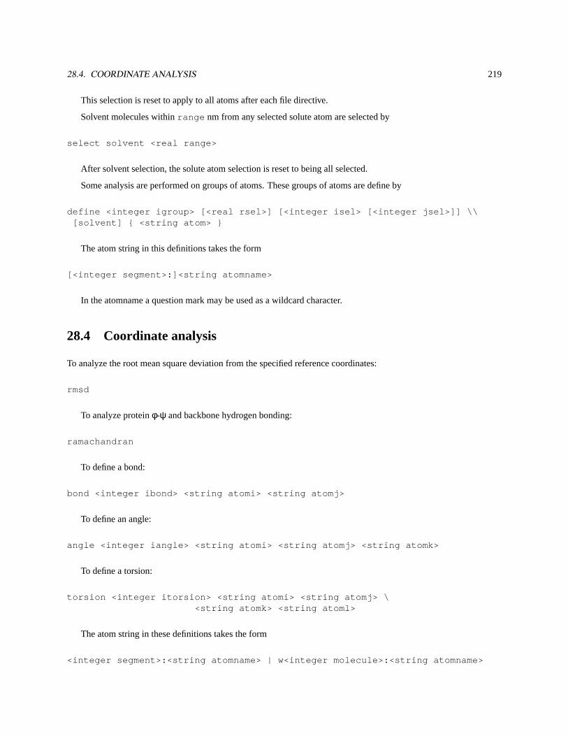
28.4. COORDINATE ANALYSIS 219
This selection is reset to apply to all atoms after each file directive.
Solvent molecules withinrange nm from any selected solute atom are selected by
select solvent <real range>
After solvent selection, the solute atom selection is reset to being all selected.
Some analysis are performed on groups of atoms. These groups of atoms are define by
define <integer igroup> [<real rsel>] [<integer isel> [<integer jsel>]] \\[solvent] { <string atom> }
The atom string in this definitions takes the form
[<integer segment>:]<string atomname>
In the atomname a question mark may be used as a wildcard character.
28.4 Coordinate analysis
To analyze the root mean square deviation from the specified reference coordinates:
rmsd
To analyze proteinφ-ψ and backbone hydrogen bonding:
ramachandran
To define a bond:
bond <integer ibond> <string atomi> <string atomj>
To define an angle:
angle <integer iangle> <string atomi> <string atomj> <string atomk>
To define a torsion:
torsion <integer itorsion> <string atomi> <string atomj> \<string atomk> <string atoml>
The atom string in these definitions takes the form
<integer segment>:<string atomname> | w<integer molecule>:<string atomname>
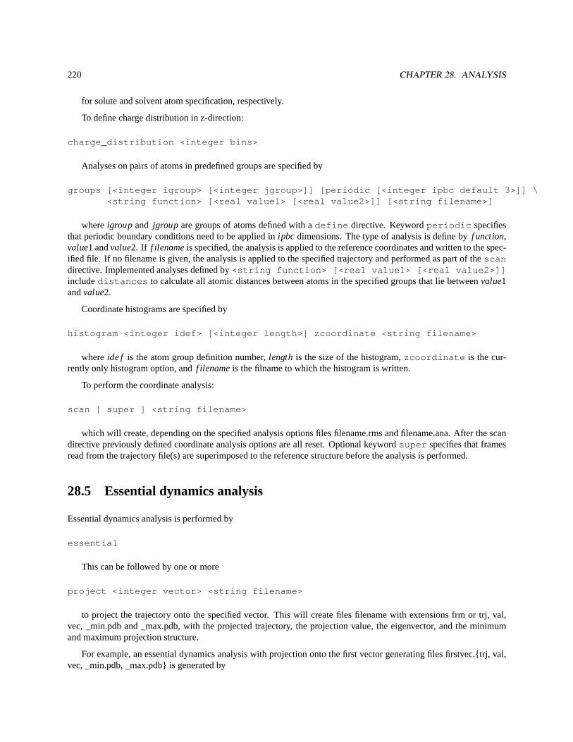
220 CHAPTER 28. ANALYSIS
for solute and solvent atom specification, respectively.
To define charge distribution in z-direction:
charge_distribution <integer bins>
Analyses on pairs of atoms in predefined groups are specified by
groups [<integer igroup> [<integer jgroup>]] [periodic [<integer ipbc default 3>]] \<string function> [<real value1> [<real value2>]] [<string filename>]
whereigroup and jgroup are groups of atoms defined with adefine directive. Keywordperiodic specifiesthat periodic boundary conditions need to be applied inipbc dimensions. The type of analysis is define byf unction,value1 andvalue2. If f ilenameis specified, the analysis is applied to the reference coordinates and written to the spec-ified file. If no filename is given, the analysis is applied to the specified trajectory and performed as part of thescandirective. Implemented analyses defined by<string function> [<real value1> [<real value2>]]includedistances to calculate all atomic distances between atoms in the specified groups that lie betweenvalue1andvalue2.
Coordinate histograms are specified by
histogram <integer idef> [<integer length>] zcoordinate <string filename>
whereide f is the atom group definition number,length is the size of the histogram,zcoordinate is the cur-rently only histogram option, andf ilenameis the filname to which the histogram is written.
To perform the coordinate analysis:
scan [ super ] <string filename>
which will create, depending on the specified analysis options files filename.rms and filename.ana. After the scandirective previously defined coordinate analysis options are all reset. Optional keywordsuper specifies that framesread from the trajectory file(s) are superimposed to the reference structure before the analysis is performed.
28.5 Essential dynamics analysis
Essential dynamics analysis is performed by
essential
This can be followed by one or more
project <integer vector> <string filename>
to project the trajectory onto the specified vector. This will create files filename with extensions frm or trj, val,vec, _min.pdb and _max.pdb, with the projected trajectory, the projection value, the eigenvector, and the minimumand maximum projection structure.
For example, an essential dynamics analysis with projection onto the first vector generating files firstvec.{trj, val,vec, _min.pdb, _max.pdb} is generated by
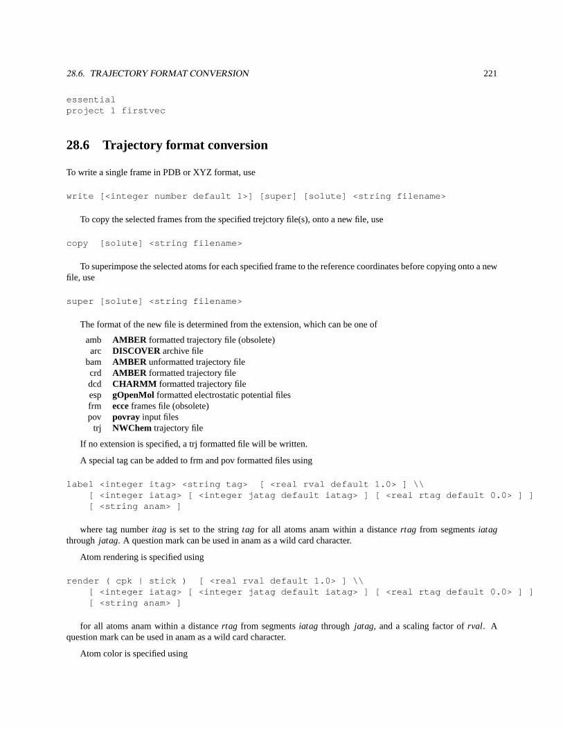
28.6. TRAJECTORY FORMAT CONVERSION 221
essentialproject 1 firstvec
28.6 Trajectory format conversion
To write a single frame in PDB or XYZ format, use
write [<integer number default 1>] [super] [solute] <string filename>
To copy the selected frames from the specified trejctory file(s), onto a new file, use
copy [solute] <string filename>
To superimpose the selected atoms for each specified frame to the reference coordinates before copying onto a newfile, use
super [solute] <string filename>
The format of the new file is determined from the extension, which can be one of
amb AMBER formatted trajectory file (obsolete)arc DISCOVER archive file
bam AMBER unformatted trajectory filecrd AMBER formatted trajectory filedcd CHARMM formatted trajectory fileesp gOpenMol formatted electrostatic potential filesfrm ecceframes file (obsolete)pov povray input files
trj NWChem trajectory file
If no extension is specified, a trj formatted file will be written.
A special tag can be added to frm and pov formatted files using
label <integer itag> <string tag> [ <real rval default 1.0> ] \\[ <integer iatag> [ <integer jatag default iatag> ] [ <real rtag default 0.0> ] ][ <string anam> ]
where tag numberitag is set to the stringtag for all atoms anam within a distancertag from segmentsiatagthrough jatag. A question mark can be used in anam as a wild card character.
Atom rendering is specified using
render ( cpk | stick ) [ <real rval default 1.0> ] \\[ <integer iatag> [ <integer jatag default iatag> ] [ <real rtag default 0.0> ] ][ <string anam> ]
for all atoms anam within a distancertag from segmentsiatag through jatag, and a scaling factor ofrval. Aquestion mark can be used in anam as a wild card character.
Atom color is specified using
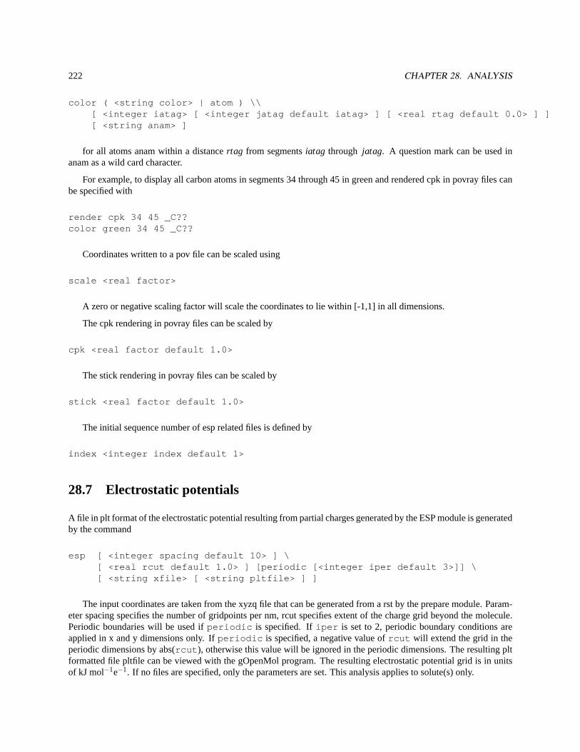
222 CHAPTER 28. ANALYSIS
color ( <string color> | atom ) \\[ <integer iatag> [ <integer jatag default iatag> ] [ <real rtag default 0.0> ] ][ <string anam> ]
for all atoms anam within a distancertag from segmentsiatag through jatag. A question mark can be used inanam as a wild card character.
For example, to display all carbon atoms in segments 34 through 45 in green and rendered cpk in povray files canbe specified with
render cpk 34 45 _C??color green 34 45 _C??
Coordinates written to a pov file can be scaled using
scale <real factor>
A zero or negative scaling factor will scale the coordinates to lie within [-1,1] in all dimensions.
The cpk rendering in povray files can be scaled by
cpk <real factor default 1.0>
The stick rendering in povray files can be scaled by
stick <real factor default 1.0>
The initial sequence number of esp related files is defined by
index <integer index default 1>
28.7 Electrostatic potentials
A file in plt format of the electrostatic potential resulting from partial charges generated by the ESP module is generatedby the command
esp [ <integer spacing default 10> ] \[ <real rcut default 1.0> ] [periodic [<integer iper default 3>]] \[ <string xfile> [ <string pltfile> ] ]
The input coordinates are taken from the xyzq file that can be generated from a rst by the prepare module. Param-eter spacing specifies the number of gridpoints per nm, rcut specifies extent of the charge grid beyond the molecule.Periodic boundaries will be used ifperiodic is specified. Ifiper is set to 2, periodic boundary conditions areapplied in x and y dimensions only. Ifperiodic is specified, a negative value ofrcut will extend the grid in theperiodic dimensions by abs(rcut ), otherwise this value will be ignored in the periodic dimensions. The resulting pltformatted file pltfile can be viewed with the gOpenMol program. The resulting electrostatic potential grid is in unitsof kJ mol−1e−1. If no files are specified, only the parameters are set. This analysis applies to solute(s) only.
Chapter 29
Combined quantum and molecularmechanics
Combined or hybrid Quantum Mechanics and Molecular Mechanics (QM/MM) is a simulation methodology that isabout 15 years old but in all the literature there are cautions that calibration computations must be done to validate themodel for each particular chemical system studied. This is not a black box style computation and the NWChem usersare advised that without calibration QM/MM may not give the appropriate results1.
The QM/MM module in NWChem is driven by the molecular dynamics module. This module currently works forany QM method that has analytic gradients2. The input for this requires the definition of chemical system via the sameinterface that is used by the MD module (c.f. Section 27). The extensions to this interface include the definition of“Quantum” atoms and “Link” where appropriate. The QM information must be present in the traditional NWCheminput deck except for the geometry3. The geometrical information will be constructed automatically by nwmd. Fordynamics and free energy simulations the input is again identical to that for nwmd with limitations on the kinds ofsimulations that can be done.
The QM/MM module is invoked with the task directive where the “theory” is QMMM. The recognized operationson the QM/MM theory directive are energy, optimize, and dynamics.
TASK QMMM (energy | optimize | dynamics)
Tasksgradient , saddle , frequencies andthermodynamics are currently not available in the QM/MMmode.
The QM/MM input consists of the standard NWChem input block:
QMMM...
END
1c.f., Singh and Kollman, J. Comp. Chem.7, 718 (1986); M. J. Field, P. A. Bash and M. Karplus, J. Comp. Chem.11, 700, (1990); J. Gao,“Methods and Applications of Combined Quantum Mechanical and Molecular Mechanical Potentials.” InReviews in Computational Chemistry;K. B. Lipkowitz, D. B. Boyd, Eds.; VCH Publishers: New York; Vol. 7, pp 119-185 (1995); and M. A. Thompson and G. K. Schenter, J. Phys.Chem996374 (1995)
2The QM/MM method will work with numerical gradients available in NWChem, but it is expected that the performance will not allow anysubstantive simulations
3Any geometry information in the traditional form will be ignored
223
224 CHAPTER 29. COMBINED QUANTUM AND MOLECULAR MECHANICS
The QMMMhas the following the additional sub-directive that the user may specify for the particular simulation.These options currently are:
29.1 EATOMS
There is one compound input directive that must exist for the QM/MM simulation to proceed. This sets the relativezero of energy for the QM component of the system. It is not incorrect to leave this value as zero but the energeticsof the QM system will likely over shadow the MM component of the system. Properties based on energy fluctuationsof the system will be overly sensitive to the energy of the QM component of the system. The zero of energy for theMM system is by definition of most parameterized force fields the separated atom energy. The zero of energy for QMsystems by definition of most QM methods is the vacuum. Thea priori determination of the separated atom energy fora particular QM method is not well defined and thus leads to a number of assumptions or guess work depending uponthe particular QM method being utilized. Therefor, the determination of the QM separated atom energy (“eatoms”) isleft to the user. The input takes the form:
EATOMS <real eatoms>
There is no default for this and the inputmust be present for a QM/MM simulation.
All other parameters that control the QM/MM simulation are set via the input to nwmd (see chapter 27).

Chapter 30
File formats
225
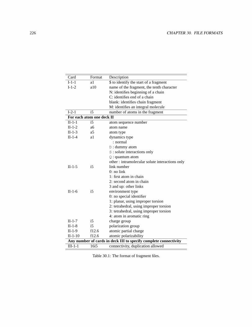
226 CHAPTER 30. FILE FORMATS
Card Format DescriptionI-1-1 a1 $ to identify the start of a fragmentI-1-2 a10 name of the fragment, the tenth character
N: identifies beginning of a chainC: identifies end of a chainblank: identifies chain fragmentM: identifies an integral molecule
I-2-1 i5 number of atoms in the fragmentFor each atom one deck IIII-1-1 i5 atom sequence numberII-1-2 a6 atom nameII-1-3 a5 atom typeII-1-4 a1 dynamics type
: normalD : dummy atomS : solute interactions onlyQ: quantum atomother : intramolecular solute interactions only
II-1-5 i5 link number0: no link1: first atom in chain2: second atom in chain3 and up: other links
II-1-6 i5 environment type0: no special identifier1: planar, using improper torsion2: tetrahedral, using improper torsion3: tetrahedral, using improper torsion4: atom in aromatic ring
II-1-7 i5 charge groupII-1-8 i5 polarization groupII-1-9 f12.6 atomic partial chargeII-1-10 f12.6 atomic polarizabilityAny number of cards in deck III to specify complete connectivityIII-1-1 16i5 connectivity, duplication allowed
Table 30.1: The format of fragment files.
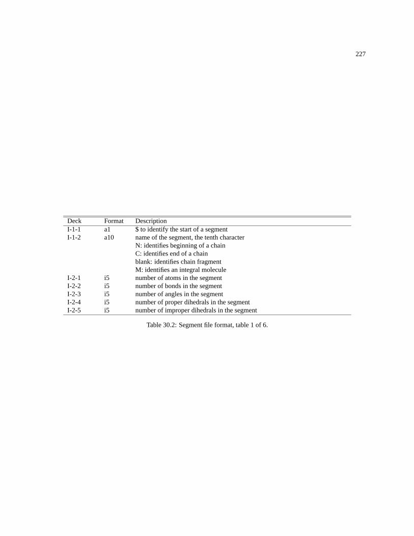
227
Deck Format DescriptionI-1-1 a1 $ to identify the start of a segmentI-1-2 a10 name of the segment, the tenth character
N: identifies beginning of a chainC: identifies end of a chainblank: identifies chain fragmentM: identifies an integral molecule
I-2-1 i5 number of atoms in the segmentI-2-2 i5 number of bonds in the segmentI-2-3 i5 number of angles in the segmentI-2-4 i5 number of proper dihedrals in the segmentI-2-5 i5 number of improper dihedrals in the segment
Table 30.2: Segment file format, table 1 of 6.
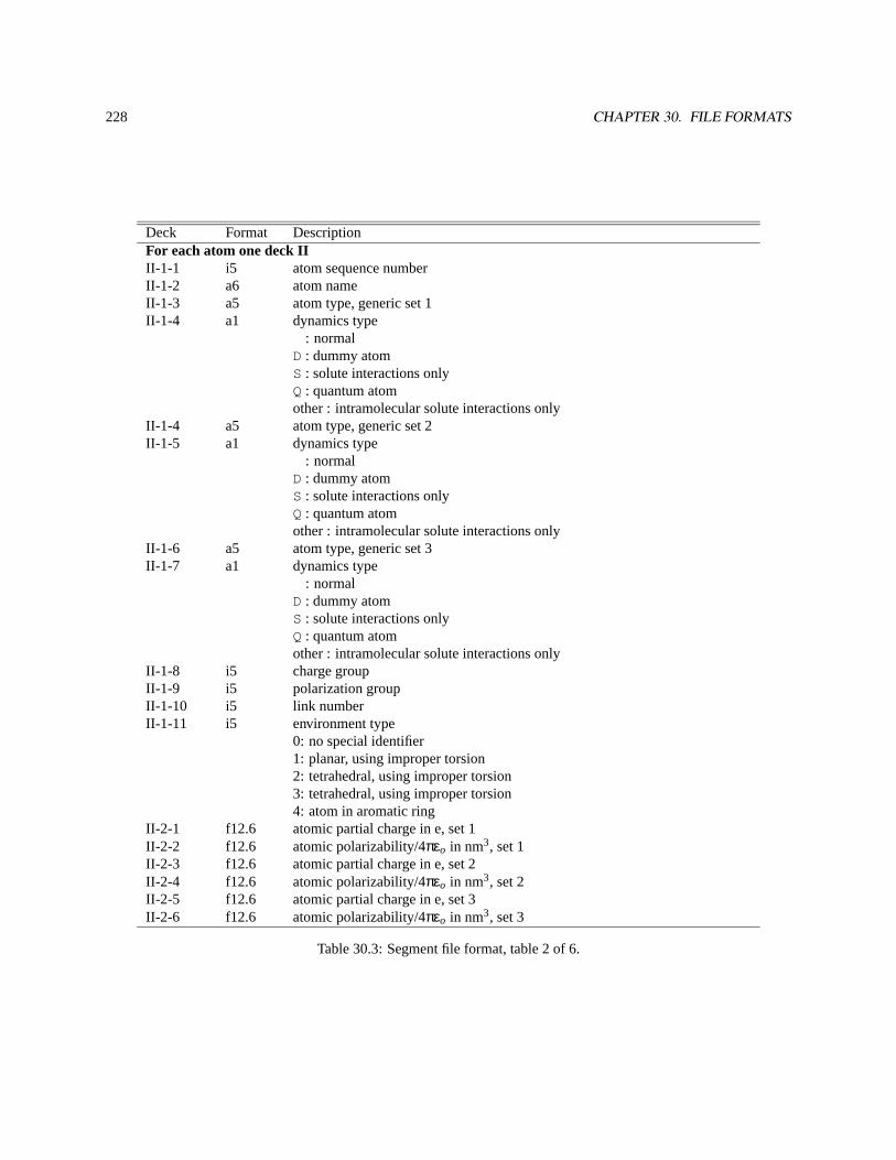
228 CHAPTER 30. FILE FORMATS
Deck Format DescriptionFor each atom one deck IIII-1-1 i5 atom sequence numberII-1-2 a6 atom nameII-1-3 a5 atom type, generic set 1II-1-4 a1 dynamics type
: normalD : dummy atomS : solute interactions onlyQ: quantum atomother : intramolecular solute interactions only
II-1-4 a5 atom type, generic set 2II-1-5 a1 dynamics type
: normalD : dummy atomS : solute interactions onlyQ: quantum atomother : intramolecular solute interactions only
II-1-6 a5 atom type, generic set 3II-1-7 a1 dynamics type
: normalD : dummy atomS : solute interactions onlyQ: quantum atomother : intramolecular solute interactions only
II-1-8 i5 charge groupII-1-9 i5 polarization groupII-1-10 i5 link numberII-1-11 i5 environment type
0: no special identifier1: planar, using improper torsion2: tetrahedral, using improper torsion3: tetrahedral, using improper torsion4: atom in aromatic ring
II-2-1 f12.6 atomic partial charge in e, set 1II-2-2 f12.6 atomic polarizability/4πεo in nm3, set 1II-2-3 f12.6 atomic partial charge in e, set 2II-2-4 f12.6 atomic polarizability/4πεo in nm3, set 2II-2-5 f12.6 atomic partial charge in e, set 3II-2-6 f12.6 atomic polarizability/4πεo in nm3, set 3
Table 30.3: Segment file format, table 2 of 6.
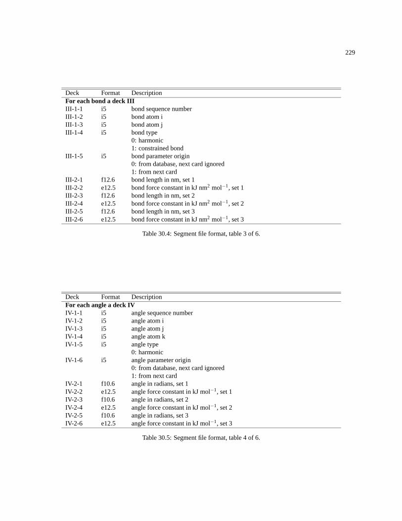
229
Deck Format DescriptionFor each bond a deck IIIIII-1-1 i5 bond sequence numberIII-1-2 i5 bond atom iIII-1-3 i5 bond atom jIII-1-4 i5 bond type
0: harmonic1: constrained bond
III-1-5 i5 bond parameter origin0: from database, next card ignored1: from next card
III-2-1 f12.6 bond length in nm, set 1III-2-2 e12.5 bond force constant in kJ nm2 mol−1, set 1III-2-3 f12.6 bond length in nm, set 2III-2-4 e12.5 bond force constant in kJ nm2 mol−1, set 2III-2-5 f12.6 bond length in nm, set 3III-2-6 e12.5 bond force constant in kJ nm2 mol−1, set 3
Table 30.4: Segment file format, table 3 of 6.
Deck Format DescriptionFor each angle a deck IVIV-1-1 i5 angle sequence numberIV-1-2 i5 angle atom iIV-1-3 i5 angle atom jIV-1-4 i5 angle atom kIV-1-5 i5 angle type
0: harmonicIV-1-6 i5 angle parameter origin
0: from database, next card ignored1: from next card
IV-2-1 f10.6 angle in radians, set 1IV-2-2 e12.5 angle force constant in kJ mol−1, set 1IV-2-3 f10.6 angle in radians, set 2IV-2-4 e12.5 angle force constant in kJ mol−1, set 2IV-2-5 f10.6 angle in radians, set 3IV-2-6 e12.5 angle force constant in kJ mol−1, set 3
Table 30.5: Segment file format, table 4 of 6.
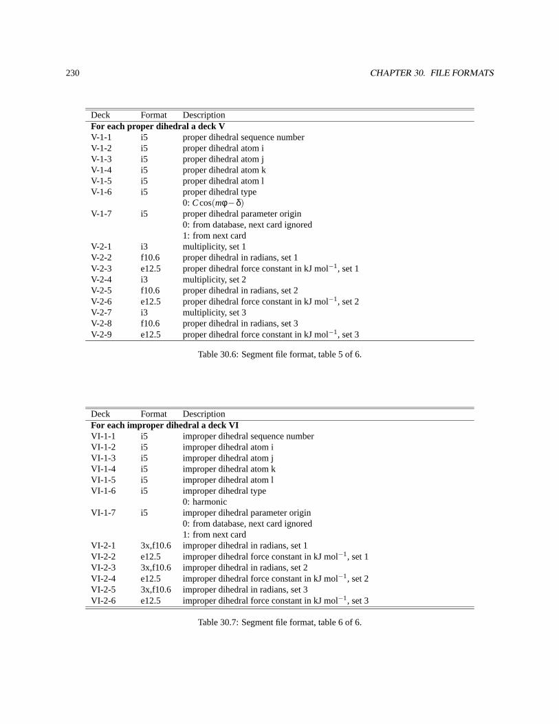
230 CHAPTER 30. FILE FORMATS
Deck Format DescriptionFor each proper dihedral a deck VV-1-1 i5 proper dihedral sequence numberV-1-2 i5 proper dihedral atom iV-1-3 i5 proper dihedral atom jV-1-4 i5 proper dihedral atom kV-1-5 i5 proper dihedral atom lV-1-6 i5 proper dihedral type
0: Ccos(mφ−δ)V-1-7 i5 proper dihedral parameter origin
0: from database, next card ignored1: from next card
V-2-1 i3 multiplicity, set 1V-2-2 f10.6 proper dihedral in radians, set 1V-2-3 e12.5 proper dihedral force constant in kJ mol−1, set 1V-2-4 i3 multiplicity, set 2V-2-5 f10.6 proper dihedral in radians, set 2V-2-6 e12.5 proper dihedral force constant in kJ mol−1, set 2V-2-7 i3 multiplicity, set 3V-2-8 f10.6 proper dihedral in radians, set 3V-2-9 e12.5 proper dihedral force constant in kJ mol−1, set 3
Table 30.6: Segment file format, table 5 of 6.
Deck Format DescriptionFor each improper dihedral a deck VIVI-1-1 i5 improper dihedral sequence numberVI-1-2 i5 improper dihedral atom iVI-1-3 i5 improper dihedral atom jVI-1-4 i5 improper dihedral atom kVI-1-5 i5 improper dihedral atom lVI-1-6 i5 improper dihedral type
0: harmonicVI-1-7 i5 improper dihedral parameter origin
0: from database, next card ignored1: from next card
VI-2-1 3x,f10.6 improper dihedral in radians, set 1VI-2-2 e12.5 improper dihedral force constant in kJ mol−1, set 1VI-2-3 3x,f10.6 improper dihedral in radians, set 2VI-2-4 e12.5 improper dihedral force constant in kJ mol−1, set 2VI-2-5 3x,f10.6 improper dihedral in radians, set 3VI-2-6 e12.5 improper dihedral force constant in kJ mol−1, set 3
Table 30.7: Segment file format, table 6 of 6.
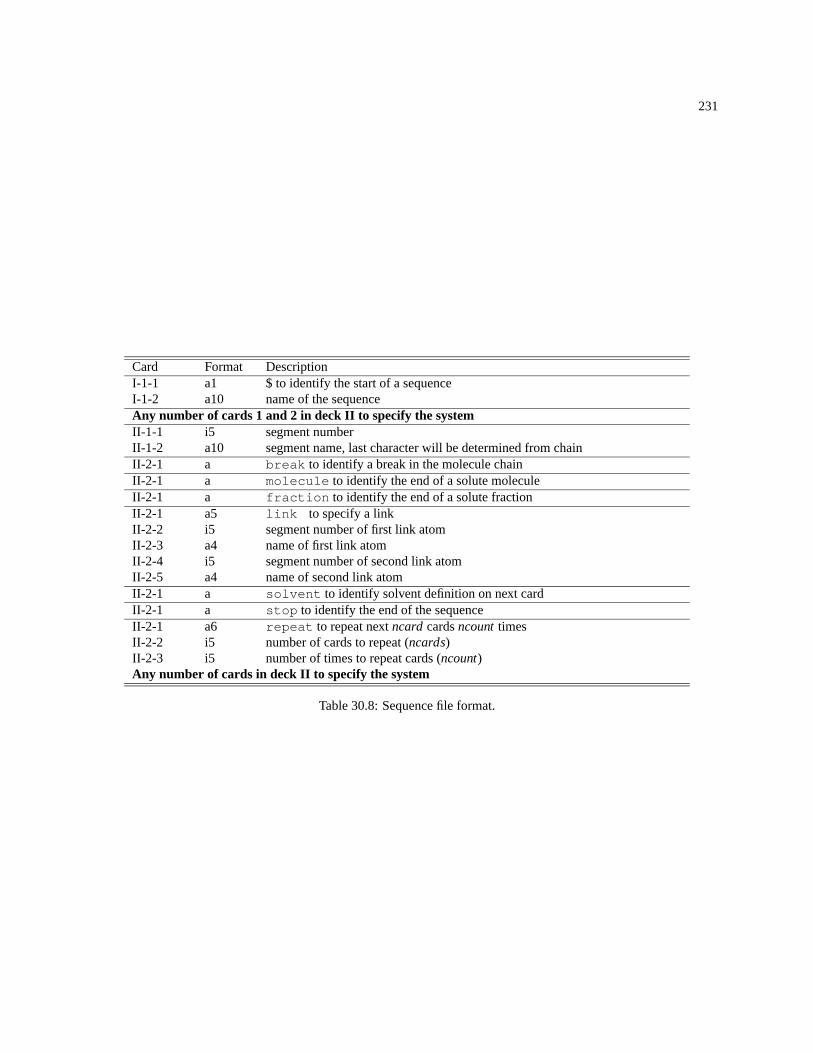
231
Card Format DescriptionI-1-1 a1 $ to identify the start of a sequenceI-1-2 a10 name of the sequenceAny number of cards 1 and 2 in deck II to specify the systemII-1-1 i5 segment numberII-1-2 a10 segment name, last character will be determined from chainII-2-1 a break to identify a break in the molecule chainII-2-1 a molecule to identify the end of a solute moleculeII-2-1 a fraction to identify the end of a solute fractionII-2-1 a5 link to specify a linkII-2-2 i5 segment number of first link atomII-2-3 a4 name of first link atomII-2-4 i5 segment number of second link atomII-2-5 a4 name of second link atomII-2-1 a solvent to identify solvent definition on next cardII-2-1 a stop to identify the end of the sequenceII-2-1 a6 repeat to repeat nextncardcardsncounttimesII-2-2 i5 number of cards to repeat (ncards)II-2-3 i5 number of times to repeat cards (ncount)Any number of cards in deck II to specify the system
Table 30.8: Sequence file format.
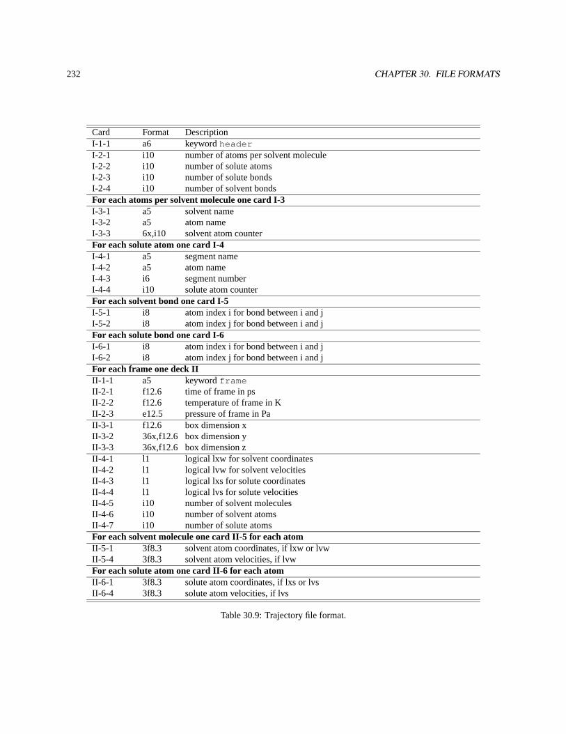
232 CHAPTER 30. FILE FORMATS
Card Format DescriptionI-1-1 a6 keywordheaderI-2-1 i10 number of atoms per solvent moleculeI-2-2 i10 number of solute atomsI-2-3 i10 number of solute bondsI-2-4 i10 number of solvent bondsFor each atoms per solvent molecule one card I-3I-3-1 a5 solvent nameI-3-2 a5 atom nameI-3-3 6x,i10 solvent atom counterFor each solute atom one card I-4I-4-1 a5 segment nameI-4-2 a5 atom nameI-4-3 i6 segment numberI-4-4 i10 solute atom counterFor each solvent bond one card I-5I-5-1 i8 atom index i for bond between i and jI-5-2 i8 atom index j for bond between i and jFor each solute bond one card I-6I-6-1 i8 atom index i for bond between i and jI-6-2 i8 atom index j for bond between i and jFor each frame one deck IIII-1-1 a5 keywordframeII-2-1 f12.6 time of frame in psII-2-2 f12.6 temperature of frame in KII-2-3 e12.5 pressure of frame in PaII-3-1 f12.6 box dimension xII-3-2 36x,f12.6 box dimension yII-3-3 36x,f12.6 box dimension zII-4-1 l1 logical lxw for solvent coordinatesII-4-2 l1 logical lvw for solvent velocitiesII-4-3 l1 logical lxs for solute coordinatesII-4-4 l1 logical lvs for solute velocitiesII-4-5 i10 number of solvent moleculesII-4-6 i10 number of solvent atomsII-4-7 i10 number of solute atomsFor each solvent molecule one card II-5 for each atomII-5-1 3f8.3 solvent atom coordinates, if lxw or lvwII-5-4 3f8.3 solvent atom velocities, if lvwFor each solute atom one card II-6 for each atomII-6-1 3f8.3 solute atom coordinates, if lxs or lvsII-6-4 3f8.3 solute atom velocities, if lvs
Table 30.9: Trajectory file format.
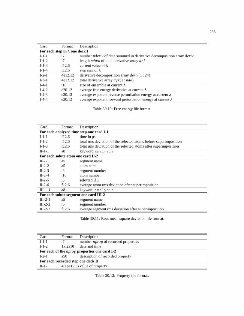
233
Card Format DescriptionFor each step inλ one deck II-1-1 i7 numbernderivof data summed in derivative decomposition arrayderivI-1-2 i7 lengthndataof total derivative arraydr fI-1-3 f12.6 current value ofλI-1-4 f12.6 step size ofλI-2-1 4e12.12 derivative decomposition arrayderiv(1 : 24)I-3-1 4e12.12 total derivative arrayd f r(1 : nda)I-4-1 i10 size of ensemble at currentλI-4-2 e20.12 average free energy derivative at currentλI-4-3 e20.12 average exponent reverse perturbation energy at currentλI-4-4 e20.12 average exponent forward perturbation energy at currentλ
Table 30.10: Free energy file format.
Card Format DescriptionFor each analyzed time step one card I-1I-1-1 f12.6 time in psI-1-2 f12.6 total rms deviation of the selected atoms before superimpositionI-1-3 f12.6 total rms deviation of the selected atoms after superimpositionII-1-1 a8 keywordanalysisFor each solute atom one card II-2II-2-1 a5 segment nameII-2-2 a5 atom nameII-2-3 i6 segment numberII-2-4 i10 atom numberII-2-5 i5 selected if 1II-2-6 f12.6 average atom rms deviation after superimpositionIII-1-1 a8 keywordanalysisFor each solute segment one card III-2III-2-1 a5 segment nameIII-2-2 i6 segment numberIII-2-3 f12.6 average segment rms deviation after superimposition
Table 30.11: Root mean square deviation file format.
Card Format DescriptionI-1-1 i7 numbernpropof recorded propertiesI-1-2 1x,2a10 date and timeFor each of thenpropproperties one card I-2I-2-1 a50 description of recorded propertyFor each recorded step one deck IIII-1-1 4(1pe12.5) value of property
Table 30.12: Property file format.

234 CHAPTER 30. FILE FORMATS
Chapter 31
Pseudopotential Plane-Wave DFT (PSPW)
A pseudopotential plane-wave (PSPW) module, which can perform Car-Parrinello simulations, is being implementedinto the NWChem program package. This module complements the capabilities of the more traditional Gaussian func-tion based approaches by including code which allows for the calculation of density functional theory total energiesand forces with the technology based on plane-wave basis sets and pseudopotentials. Consistent with NWChem’sphilosophy this module is able to run on a variety of architectures, including parallel supercomputers.
The advantage of a PSPW method is that it has been shown to have an accuracy close to chemical accuracy formany applications, yet is still fast enough to treat systems containing hundreds of atoms. Another significant advantageis its ability to simulate dynamics on a ground state potential surface directly at run-time. This method’s efficiencyand accuracy make it a desirable first principles method of simulation in the study of complex molecular, liquid, andsolid state systems. Applications for this first principles method include the calculation of free energies, search forglobal minima, explicit simulation of solvated molecules, and simulations of complex vibrational modes that cannotbe described within the harmonic approximation.
Section 31.1 describes the tasks contained within the PSPW module. The RTDB entries and datafiles used by thePSPW module are described in section 31.2. Car-Parrinello output data files are described in section 31.2.9, and theminimization and Car-Parrinello algorithms are described in sections 31.3-31.4. Examples of how to setup and run asteepest descent simulation and a Car-Parrinello simulation are presented in sections 31.5-31.6. Finally in section 31.7the capabilities and limitations of the PSPW module are discussed.
If you are a first time user of this module it is recommended that you skip the next five sections and proceed directlyto the tutorials in sections 31.5-31.6.
31.1 PSPW Tasks
All input to the PSPW Tasks is contained within the compound PSPW block,
PSPW...
END
To perform an actual calculation a TASK PSPW directive is used. The TASK cg_pspw directive may also be used(see below). The format for the TASK PSPW directive is the TASK directive followed by the PSPW string, and afterthat an<operation> string is required. The TASK PSPW directive for PSPW calculations is of the following form:
235
236 CHAPTER 31. PSEUDOPOTENTIAL PLANE-WAVE DFT (PSPW)
TASK PSPW [steepest_descent ||conjugate_gradient ||Car-Parrinello ||psp_formatter ||wavefunction_initializer ||v_wavefunction_initializer ||wavefunction_expander ||psp_generator ||(no default)]
Currently available tasks are listed. Note that unlike most NWChem modules, the PSPW module does not contain anenergy operation. This means that there is no default operation and hence an operation must always be specified.
PSPW tasks are of two types. The first type of task is used to setup or change needed data files for a PSPWsimulation. Tasks of this type are psp_formatter, wavefunction_initializer, v_wavefunction_initializer, wavefunc-tion_expander, and psp_generator. The second type of task is used to actually run a PSPW simulation. Tasks ofthis type are steepest_descent, and Car-Parrinello. The following subsections describe the input to these tasks.
The PSPW module is also interfaced to driver, stepper, and freqency task operations through the cg_pspw theorydirective, see section 5.10.1. The PSPW conjugate_gradient sub-module is used in this interface. Specifically thefollowing task operations are interafaced using the cg_pspw theory directive.
TASK cg_pspw energy #equivalent to TASK PSPW conjugate_gradientTASK cg_pspw gradientTASK cg_pspw optimizeTASK cg_pspw saddleTASK cg_pspw freqenciesTASK cg_pspw vib
31.1.1 STEEPEST_DESCENT
The steepest_descent task is used to optimize the one-electron orbitals with respect to the total energy. In addition itcan also be used to optimize geometries. This method is meant to be used for coarse optimization of the one-electronorbitals. A detailed description of the this method is described in section 31.3.1
Input to the steepest_descent simulation is contained within the steepest_descent sub-block.
PSPW...STEEPEST_DESCENT
...END...
END
To run a steepest_descent calculation the following directive is used:
TASK PSPW steepest_descent
The steepest_descent sub-block contains a great deal of input, including pointers to data, as well as parameter input.Listed below is the format of a STEEPEST_DESCENT sub-block.
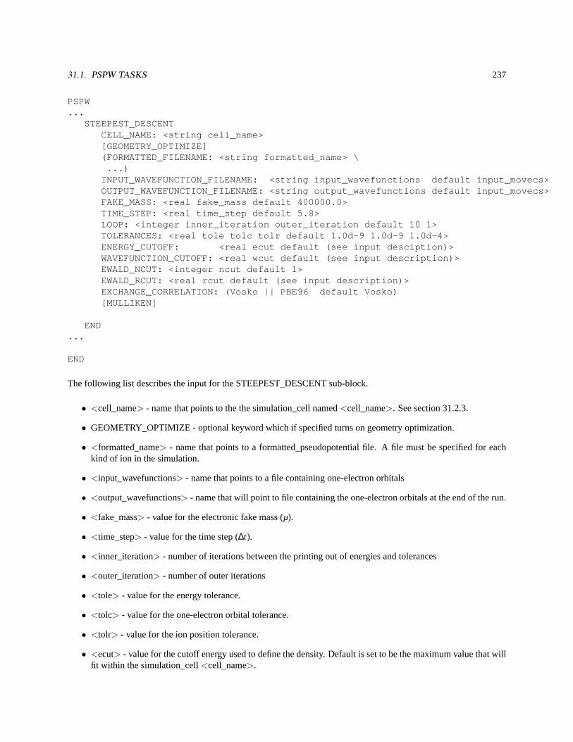
31.1. PSPW TASKS 237
PSPW...
STEEPEST_DESCENTCELL_NAME: <string cell_name>[GEOMETRY_OPTIMIZE](FORMATTED_FILENAME: <string formatted_name> \
...)INPUT_WAVEFUNCTION_FILENAME: <string input_wavefunctions default input_movecs>OUTPUT_WAVEFUNCTION_FILENAME: <string output_wavefunctions default input_movecs>FAKE_MASS: <real fake_mass default 400000.0>TIME_STEP: <real time_step default 5.8>LOOP: <integer inner_iteration outer_iteration default 10 1>TOLERANCES: <real tole tolc tolr default 1.0d-9 1.0d-9 1.0d-4>ENERGY_CUTOFF: <real ecut default (see input desciption)>WAVEFUNCTION_CUTOFF: <real wcut default (see input description)>EWALD_NCUT: <integer ncut default 1>EWALD_RCUT: <real rcut default (see input description)>EXCHANGE_CORRELATION: (Vosko || PBE96 default Vosko)[MULLIKEN]
END...
END
The following list describes the input for the STEEPEST_DESCENT sub-block.
• <cell_name> - name that points to the the simulation_cell named<cell_name>. See section 31.2.3.
• GEOMETRY_OPTIMIZE - optional keyword which if specified turns on geometry optimization.
• <formatted_name> - name that points to a formatted_pseudopotential file. A file must be specified for eachkind of ion in the simulation.
• <input_wavefunctions> - name that points to a file containing one-electron orbitals
• <output_wavefunctions> - name that will point to file containing the one-electron orbitals at the end of the run.
• <fake_mass> - value for the electronic fake mass (µ).
• <time_step> - value for the time step (∆t).
• <inner_iteration> - number of iterations between the printing out of energies and tolerances
• <outer_iteration> - number of outer iterations
• <tole> - value for the energy tolerance.
• <tolc> - value for the one-electron orbital tolerance.
• <tolr> - value for the ion position tolerance.
• <ecut> - value for the cutoff energy used to define the density. Default is set to be the maximum value that willfit within the simulation_cell<cell_name>.
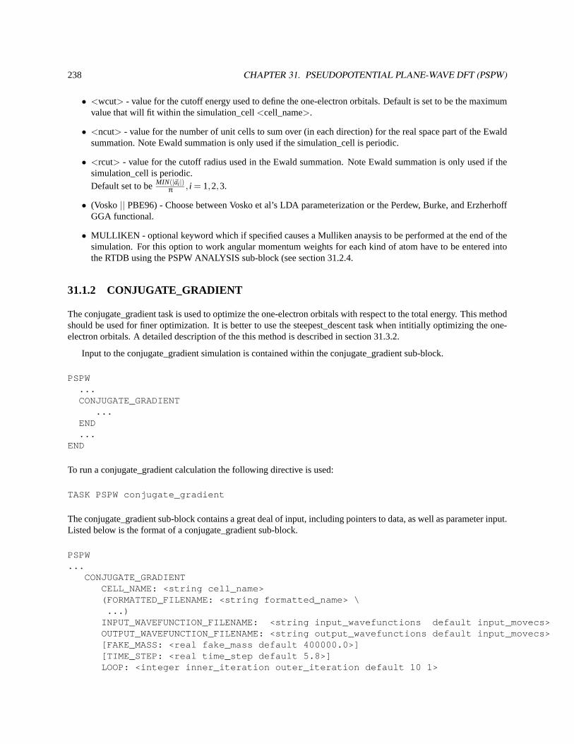
238 CHAPTER 31. PSEUDOPOTENTIAL PLANE-WAVE DFT (PSPW)
• <wcut> - value for the cutoff energy used to define the one-electron orbitals. Default is set to be the maximumvalue that will fit within the simulation_cell<cell_name>.
• <ncut> - value for the number of unit cells to sum over (in each direction) for the real space part of the Ewaldsummation. Note Ewald summation is only used if the simulation_cell is periodic.
• <rcut> - value for the cutoff radius used in the Ewald summation. Note Ewald summation is only used if thesimulation_cell is periodic.Default set to beMIN(|~ai |)
π , i = 1,2,3.
• (Vosko || PBE96) - Choose between Vosko et al’s LDA parameterization or the Perdew, Burke, and ErzherhoffGGA functional.
• MULLIKEN - optional keyword which if specified causes a Mulliken anaysis to be performed at the end of thesimulation. For this option to work angular momentum weights for each kind of atom have to be entered intothe RTDB using the PSPW ANALYSIS sub-block (see section 31.2.4.
31.1.2 CONJUGATE_GRADIENT
The conjugate_gradient task is used to optimize the one-electron orbitals with respect to the total energy. This methodshould be used for finer optimization. It is better to use the steepest_descent task when intitially optimizing the one-electron orbitals. A detailed description of the this method is described in section 31.3.2.
Input to the conjugate_gradient simulation is contained within the conjugate_gradient sub-block.
PSPW...CONJUGATE_GRADIENT
...END...
END
To run a conjugate_gradient calculation the following directive is used:
TASK PSPW conjugate_gradient
The conjugate_gradient sub-block contains a great deal of input, including pointers to data, as well as parameter input.Listed below is the format of a conjugate_gradient sub-block.
PSPW...
CONJUGATE_GRADIENTCELL_NAME: <string cell_name>(FORMATTED_FILENAME: <string formatted_name> \
...)INPUT_WAVEFUNCTION_FILENAME: <string input_wavefunctions default input_movecs>OUTPUT_WAVEFUNCTION_FILENAME: <string output_wavefunctions default input_movecs>[FAKE_MASS: <real fake_mass default 400000.0>][TIME_STEP: <real time_step default 5.8>]LOOP: <integer inner_iteration outer_iteration default 10 1>
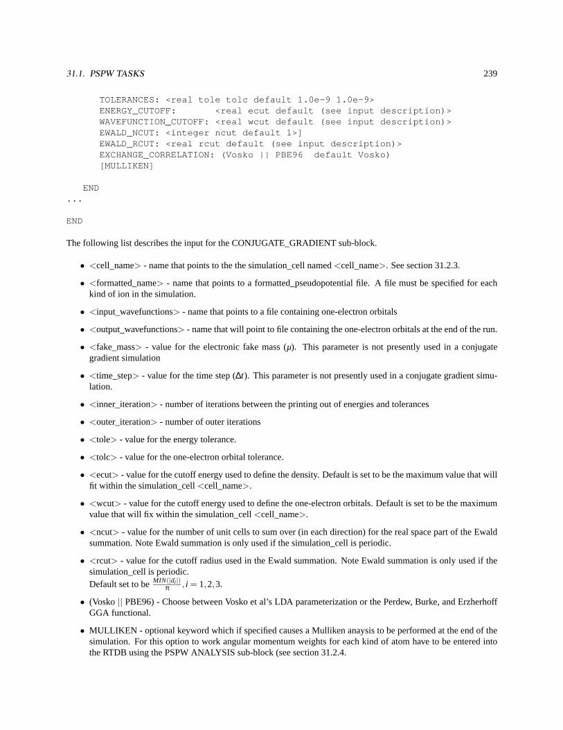
31.1. PSPW TASKS 239
TOLERANCES: <real tole tolc default 1.0e-9 1.0e-9>ENERGY_CUTOFF: <real ecut default (see input description)>WAVEFUNCTION_CUTOFF: <real wcut default (see input description)>EWALD_NCUT: <integer ncut default 1>]EWALD_RCUT: <real rcut default (see input description)>EXCHANGE_CORRELATION: (Vosko || PBE96 default Vosko)[MULLIKEN]
END...
END
The following list describes the input for the CONJUGATE_GRADIENT sub-block.
• <cell_name> - name that points to the the simulation_cell named<cell_name>. See section 31.2.3.
• <formatted_name> - name that points to a formatted_pseudopotential file. A file must be specified for eachkind of ion in the simulation.
• <input_wavefunctions> - name that points to a file containing one-electron orbitals
• <output_wavefunctions> - name that will point to file containing the one-electron orbitals at the end of the run.
• <fake_mass> - value for the electronic fake mass (µ). This parameter is not presently used in a conjugategradient simulation
• <time_step> - value for the time step (∆t). This parameter is not presently used in a conjugate gradient simu-lation.
• <inner_iteration> - number of iterations between the printing out of energies and tolerances
• <outer_iteration> - number of outer iterations
• <tole> - value for the energy tolerance.
• <tolc> - value for the one-electron orbital tolerance.
• <ecut> - value for the cutoff energy used to define the density. Default is set to be the maximum value that willfit within the simulation_cell<cell_name>.
• <wcut> - value for the cutoff energy used to define the one-electron orbitals. Default is set to be the maximumvalue that will fix within the simulation_cell<cell_name>.
• <ncut> - value for the number of unit cells to sum over (in each direction) for the real space part of the Ewaldsummation. Note Ewald summation is only used if the simulation_cell is periodic.
• <rcut> - value for the cutoff radius used in the Ewald summation. Note Ewald summation is only used if thesimulation_cell is periodic.Default set to beMIN(|~ai |)
π , i = 1,2,3.
• (Vosko || PBE96) - Choose between Vosko et al’s LDA parameterization or the Perdew, Burke, and ErzherhoffGGA functional.
• MULLIKEN - optional keyword which if specified causes a Mulliken anaysis to be performed at the end of thesimulation. For this option to work angular momentum weights for each kind of atom have to be entered intothe RTDB using the PSPW ANALYSIS sub-block (see section 31.2.4.
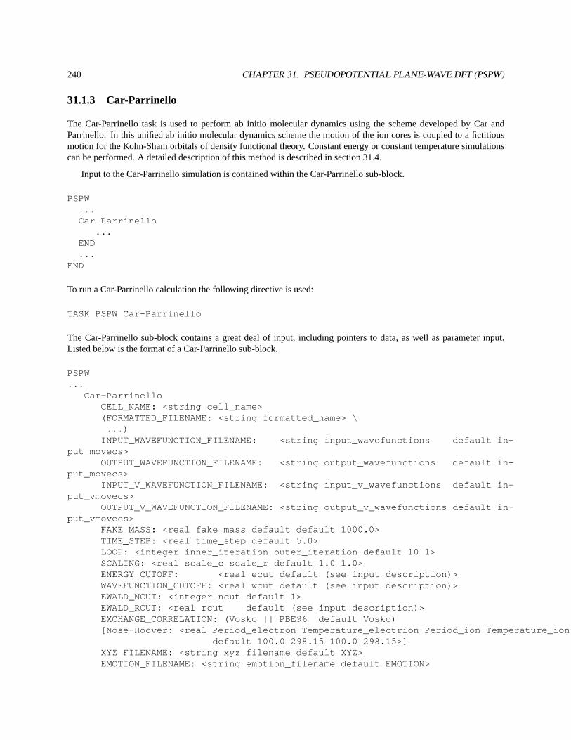
240 CHAPTER 31. PSEUDOPOTENTIAL PLANE-WAVE DFT (PSPW)
31.1.3 Car-Parrinello
The Car-Parrinello task is used to perform ab initio molecular dynamics using the scheme developed by Car andParrinello. In this unified ab initio molecular dynamics scheme the motion of the ion cores is coupled to a fictitiousmotion for the Kohn-Sham orbitals of density functional theory. Constant energy or constant temperature simulationscan be performed. A detailed description of this method is described in section 31.4.
Input to the Car-Parrinello simulation is contained within the Car-Parrinello sub-block.
PSPW...Car-Parrinello
...END...
END
To run a Car-Parrinello calculation the following directive is used:
TASK PSPW Car-Parrinello
The Car-Parrinello sub-block contains a great deal of input, including pointers to data, as well as parameter input.Listed below is the format of a Car-Parrinello sub-block.
PSPW...
Car-ParrinelloCELL_NAME: <string cell_name>(FORMATTED_FILENAME: <string formatted_name> \
...)INPUT_WAVEFUNCTION_FILENAME: <string input_wavefunctions default in-
put_movecs>OUTPUT_WAVEFUNCTION_FILENAME: <string output_wavefunctions default in-
put_movecs>INPUT_V_WAVEFUNCTION_FILENAME: <string input_v_wavefunctions default in-
put_vmovecs>OUTPUT_V_WAVEFUNCTION_FILENAME: <string output_v_wavefunctions default in-
put_vmovecs>FAKE_MASS: <real fake_mass default default 1000.0>TIME_STEP: <real time_step default 5.0>LOOP: <integer inner_iteration outer_iteration default 10 1>SCALING: <real scale_c scale_r default 1.0 1.0>ENERGY_CUTOFF: <real ecut default (see input description)>WAVEFUNCTION_CUTOFF: <real wcut default (see input description)>EWALD_NCUT: <integer ncut default 1>EWALD_RCUT: <real rcut default (see input description)>EXCHANGE_CORRELATION: (Vosko || PBE96 default Vosko)[Nose-Hoover: <real Period_electron Temperature_electrion Period_ion Temperature_ion
default 100.0 298.15 100.0 298.15>]XYZ_FILENAME: <string xyz_filename default XYZ>EMOTION_FILENAME: <string emotion_filename default EMOTION>
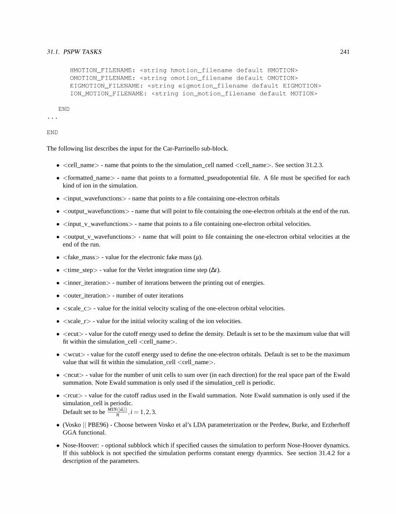
31.1. PSPW TASKS 241
HMOTION_FILENAME: <string hmotion_filename default HMOTION>OMOTION_FILENAME: <string omotion_filename default OMOTION>EIGMOTION_FILENAME: <string eigmotion_filename default EIGMOTION>ION_MOTION_FILENAME: <string ion_motion_filename default MOTION>
END...
END
The following list describes the input for the Car-Parrinello sub-block.
• <cell_name> - name that points to the the simulation_cell named<cell_name>. See section 31.2.3.
• <formatted_name> - name that points to a formatted_pseudopotential file. A file must be specified for eachkind of ion in the simulation.
• <input_wavefunctions> - name that points to a file containing one-electron orbitals
• <output_wavefunctions> - name that will point to file containing the one-electron orbitals at the end of the run.
• <input_v_wavefunctions> - name that points to a file containing one-electron orbital velocities.
• <output_v_wavefunctions> - name that will point to file containing the one-electron orbital velocities at theend of the run.
• <fake_mass> - value for the electronic fake mass (µ).
• <time_step> - value for the Verlet integration time step (∆t).
• <inner_iteration> - number of iterations between the printing out of energies.
• <outer_iteration> - number of outer iterations
• <scale_c> - value for the initial velocity scaling of the one-electron orbital velocities.
• <scale_r> - value for the initial velocity scaling of the ion velocities.
• <ecut> - value for the cutoff energy used to define the density. Default is set to be the maximum value that willfit within the simulation_cell<cell_name>.
• <wcut> - value for the cutoff energy used to define the one-electron orbitals. Default is set to be the maximumvalue that will fit within the simulation_cell<cell_name>.
• <ncut> - value for the number of unit cells to sum over (in each direction) for the real space part of the Ewaldsummation. Note Ewald summation is only used if the simulation_cell is periodic.
• <rcut> - value for the cutoff radius used in the Ewald summation. Note Ewald summation is only used if thesimulation_cell is periodic.Default set to beMIN(|~ai |)
π , i = 1,2,3.
• (Vosko || PBE96) - Choose between Vosko et al’s LDA parameterization or the Perdew, Burke, and ErzherhoffGGA functional.
• Nose-Hoover: - optional subblock which if specified causes the simulation to perform Nose-Hoover dynamics.If this subblock is not specified the simulation performs constant energy dyanmics. See section 31.4.2 for adescription of the parameters.
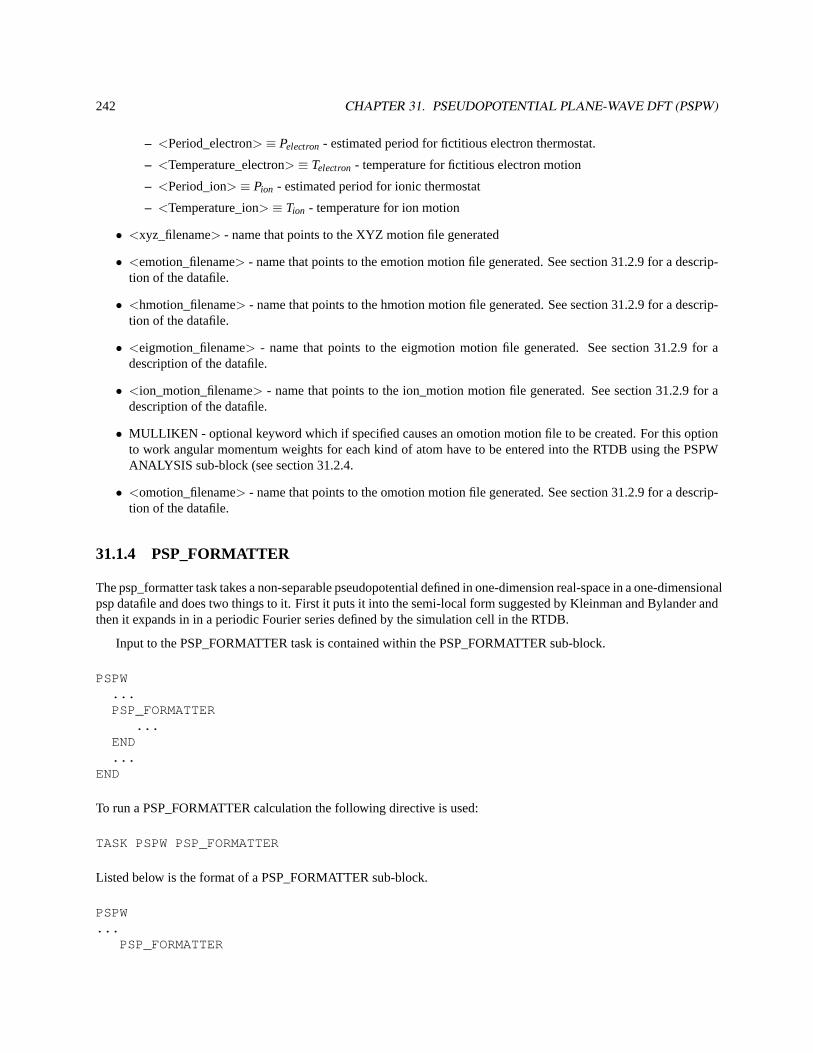
242 CHAPTER 31. PSEUDOPOTENTIAL PLANE-WAVE DFT (PSPW)
– <Period_electron> ≡ Pelectron- estimated period for fictitious electron thermostat.
– <Temperature_electron> ≡ Telectron- temperature for fictitious electron motion
– <Period_ion> ≡ Pion - estimated period for ionic thermostat
– <Temperature_ion> ≡ Tion - temperature for ion motion
• <xyz_filename> - name that points to the XYZ motion file generated
• <emotion_filename> - name that points to the emotion motion file generated. See section 31.2.9 for a descrip-tion of the datafile.
• <hmotion_filename> - name that points to the hmotion motion file generated. See section 31.2.9 for a descrip-tion of the datafile.
• <eigmotion_filename> - name that points to the eigmotion motion file generated. See section 31.2.9 for adescription of the datafile.
• <ion_motion_filename> - name that points to the ion_motion motion file generated. See section 31.2.9 for adescription of the datafile.
• MULLIKEN - optional keyword which if specified causes an omotion motion file to be created. For this optionto work angular momentum weights for each kind of atom have to be entered into the RTDB using the PSPWANALYSIS sub-block (see section 31.2.4.
• <omotion_filename> - name that points to the omotion motion file generated. See section 31.2.9 for a descrip-tion of the datafile.
31.1.4 PSP_FORMATTER
The psp_formatter task takes a non-separable pseudopotential defined in one-dimension real-space in a one-dimensionalpsp datafile and does two things to it. First it puts it into the semi-local form suggested by Kleinman and Bylander andthen it expands in in a periodic Fourier series defined by the simulation cell in the RTDB.
Input to the PSP_FORMATTER task is contained within the PSP_FORMATTER sub-block.
PSPW...PSP_FORMATTER
...END...
END
To run a PSP_FORMATTER calculation the following directive is used:
TASK PSPW PSP_FORMATTER
Listed below is the format of a PSP_FORMATTER sub-block.
PSPW...
PSP_FORMATTER
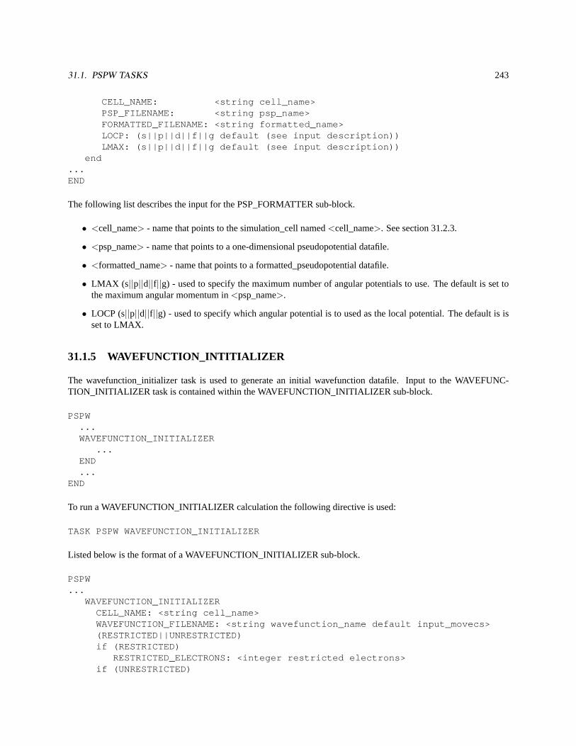
31.1. PSPW TASKS 243
CELL_NAME: <string cell_name>PSP_FILENAME: <string psp_name>FORMATTED_FILENAME: <string formatted_name>LOCP: (s||p||d||f||g default (see input description))LMAX: (s||p||d||f||g default (see input description))
end...END
The following list describes the input for the PSP_FORMATTER sub-block.
• <cell_name> - name that points to the simulation_cell named<cell_name>. See section 31.2.3.
• <psp_name> - name that points to a one-dimensional pseudopotential datafile.
• <formatted_name> - name that points to a formatted_pseudopotential datafile.
• LMAX (s ||p||d||f||g) - used to specify the maximum number of angular potentials to use. The default is set tothe maximum angular momentum in<psp_name>.
• LOCP (s||p||d||f||g) - used to specify which angular potential is to used as the local potential. The default is isset to LMAX.
31.1.5 WAVEFUNCTION_INTITIALIZER
The wavefunction_initializer task is used to generate an initial wavefunction datafile. Input to the WAVEFUNC-TION_INITIALIZER task is contained within the WAVEFUNCTION_INITIALIZER sub-block.
PSPW...WAVEFUNCTION_INITIALIZER
...END...
END
To run a WAVEFUNCTION_INITIALIZER calculation the following directive is used:
TASK PSPW WAVEFUNCTION_INITIALIZER
Listed below is the format of a WAVEFUNCTION_INITIALIZER sub-block.
PSPW...
WAVEFUNCTION_INITIALIZERCELL_NAME: <string cell_name>WAVEFUNCTION_FILENAME: <string wavefunction_name default input_movecs>(RESTRICTED||UNRESTRICTED)if (RESTRICTED)
RESTRICTED_ELECTRONS: <integer restricted electrons>if (UNRESTRICTED)
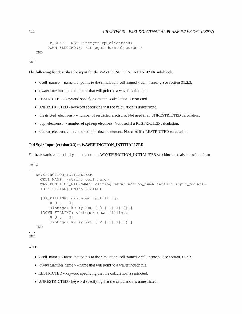
244 CHAPTER 31. PSEUDOPOTENTIAL PLANE-WAVE DFT (PSPW)
UP_ELECTRONS: <integer up_electrons>DOWN_ELECTRONS: <integer down_electrons>
END...END
The following list describes the input for the WAVEFUNCTION_INITIALIZER sub-block.
• <cell_name> - name that points to the simulation_cell named<cell_name>. See section 31.2.3.
• <wavefunction_name> - name that will point to a wavefunction file.
• RESTRICTED - keyword specifying that the calculation is restricted.
• UNRESTRICTED - keyword specifying that the calculation is unrestricted.
• <restricted_electrons> - number of restricted electrons. Not used if an UNRESTRICTED calculation.
• <up_electrons> - number of spin-up electrons. Not used if a RESTRICTED calculation.
• <down_electrons> - number of spin-down electrons. Not used if a RESTRICTED calculation.
Old Style Input (version 3.3) to WAVEFUNCTION_INTITIALIZER
For backwards compatibility, the input to the WAVEFUNCTION_INITIALIZER sub-block can also be of the form
PSPW...
WAVEFUNCTION_INITIALIZERCELL_NAME: <string cell_name>WAVEFUNCTION_FILENAME: <string wavefunction_name default input_movecs>(RESTRICTED||UNRESTRICTED)
[UP_FILLING: <integer up_filling>[0 0 0 0]{<integer kx ky kz> (-2||-1||1||2)}]
[DOWN_FILLING: <integer down_filling>[0 0 0 0]{<integer kx ky kz> (-2||-1||1||2)}]
END...END
where
• <cell_name> - name that points to the simulation_cell named<cell_name>. See section 31.2.3.
• <wavefunction_name> - name that will point to a wavefunction file.
• RESTRICTED - keyword specifying that the calculation is restricted.
• UNRESTRICTED - keyword specifying that the calculation is unrestricted.
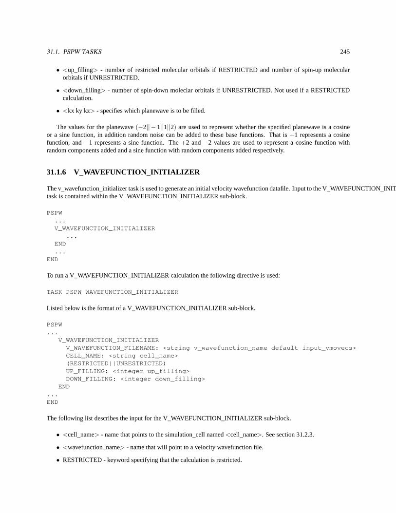
31.1. PSPW TASKS 245
• <up_filling> - number of restricted molecular orbitals if RESTRICTED and number of spin-up molecularorbitals if UNRESTRICTED.
• <down_filling> - number of spin-down moleclar orbitals if UNRESTRICTED. Not used if a RESTRICTEDcalculation.
• <kx ky kz> - specifies which planewave is to be filled.
The values for the planewave(−2|| −1||1||2) are used to represent whether the specified planewave is a cosineor a sine function, in addition random noise can be added to these base functions. That is+1 represents a cosinefunction, and−1 represents a sine function. The+2 and−2 values are used to represent a cosine function withrandom components added and a sine function with random components added respectively.
31.1.6 V_WAVEFUNCTION_INITIALIZER
The v_wavefunction_initializer task is used to generate an initial velocity wavefunction datafile. Input to the V_WAVEFUNCTION_INITIALIZERtask is contained within the V_WAVEFUNCTION_INITIALIZER sub-block.
PSPW...V_WAVEFUNCTION_INITIALIZER
...END...
END
To run a V_WAVEFUNCTION_INITIALIZER calculation the following directive is used:
TASK PSPW WAVEFUNCTION_INITIALIZER
Listed below is the format of a V_WAVEFUNCTION_INITIALIZER sub-block.
PSPW...
V_WAVEFUNCTION_INITIALIZERV_WAVEFUNCTION_FILENAME: <string v_wavefunction_name default input_vmovecs>CELL_NAME: <string cell_name>(RESTRICTED||UNRESTRICTED)UP_FILLING: <integer up_filling>DOWN_FILLING: <integer down_filling>
END...END
The following list describes the input for the V_WAVEFUNCTION_INITIALIZER sub-block.
• <cell_name> - name that points to the simulation_cell named<cell_name>. See section 31.2.3.
• <wavefunction_name> - name that will point to a velocity wavefunction file.
• RESTRICTED - keyword specifying that the calculation is restricted.
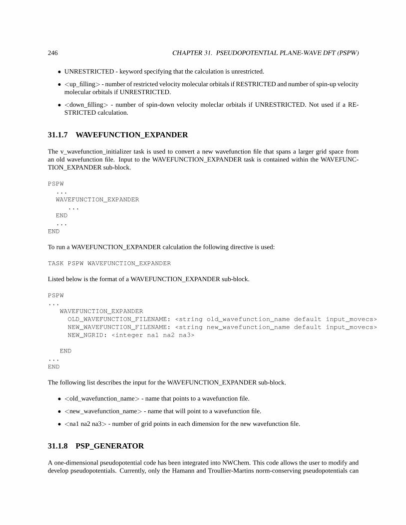
246 CHAPTER 31. PSEUDOPOTENTIAL PLANE-WAVE DFT (PSPW)
• UNRESTRICTED - keyword specifying that the calculation is unrestricted.
• <up_filling> - number of restricted velocity molecular orbitals if RESTRICTED and number of spin-up velocitymolecular orbitals if UNRESTRICTED.
• <down_filling> - number of spin-down velocity moleclar orbitals if UNRESTRICTED. Not used if a RE-STRICTED calculation.
31.1.7 WAVEFUNCTION_EXPANDER
The v_wavefunction_initializer task is used to convert a new wavefunction file that spans a larger grid space froman old wavefunction file. Input to the WAVEFUNCTION_EXPANDER task is contained within the WAVEFUNC-TION_EXPANDER sub-block.
PSPW...WAVEFUNCTION_EXPANDER
...END...
END
To run a WAVEFUNCTION_EXPANDER calculation the following directive is used:
TASK PSPW WAVEFUNCTION_EXPANDER
Listed below is the format of a WAVEFUNCTION_EXPANDER sub-block.
PSPW...
WAVEFUNCTION_EXPANDEROLD_WAVEFUNCTION_FILENAME: <string old_wavefunction_name default input_movecs>NEW_WAVEFUNCTION_FILENAME: <string new_wavefunction_name default input_movecs>NEW_NGRID: <integer na1 na2 na3>
END...END
The following list describes the input for the WAVEFUNCTION_EXPANDER sub-block.
• <old_wavefunction_name> - name that points to a wavefunction file.
• <new_wavefunction_name> - name that will point to a wavefunction file.
• <na1 na2 na3> - number of grid points in each dimension for the new wavefunction file.
31.1.8 PSP_GENERATOR
A one-dimensional pseudopotential code has been integrated into NWChem. This code allows the user to modify anddevelop pseudopotentials. Currently, only the Hamann and Troullier-Martins norm-conserving pseudopotentials can
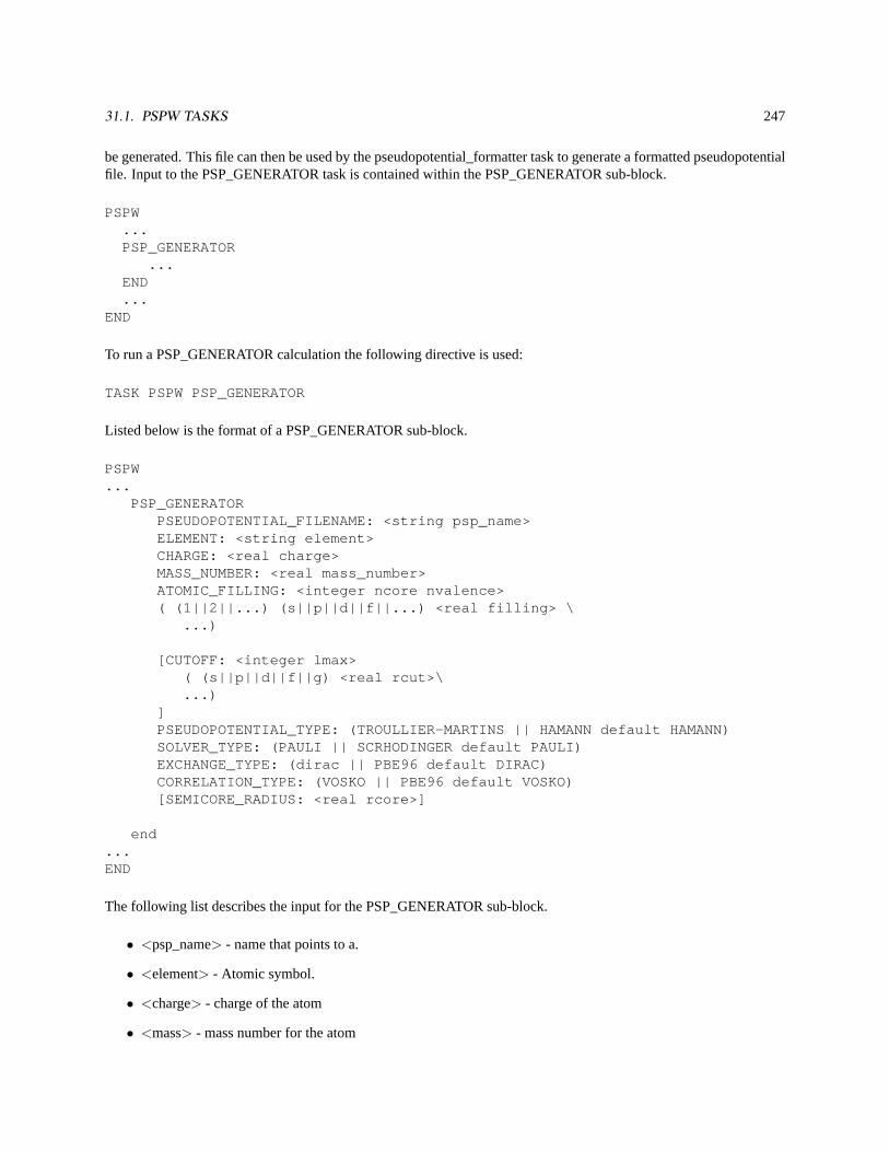
31.1. PSPW TASKS 247
be generated. This file can then be used by the pseudopotential_formatter task to generate a formatted pseudopotentialfile. Input to the PSP_GENERATOR task is contained within the PSP_GENERATOR sub-block.
PSPW...PSP_GENERATOR
...END...
END
To run a PSP_GENERATOR calculation the following directive is used:
TASK PSPW PSP_GENERATOR
Listed below is the format of a PSP_GENERATOR sub-block.
PSPW...
PSP_GENERATORPSEUDOPOTENTIAL_FILENAME: <string psp_name>ELEMENT: <string element>CHARGE: <real charge>MASS_NUMBER: <real mass_number>ATOMIC_FILLING: <integer ncore nvalence>( (1||2||...) (s||p||d||f||...) <real filling> \
...)
[CUTOFF: <integer lmax>( (s||p||d||f||g) <real rcut>\...)
]PSEUDOPOTENTIAL_TYPE: (TROULLIER-MARTINS || HAMANN default HAMANN)SOLVER_TYPE: (PAULI || SCRHODINGER default PAULI)EXCHANGE_TYPE: (dirac || PBE96 default DIRAC)CORRELATION_TYPE: (VOSKO || PBE96 default VOSKO)[SEMICORE_RADIUS: <real rcore>]
end...END
The following list describes the input for the PSP_GENERATOR sub-block.
• <psp_name> - name that points to a.
• <element> - Atomic symbol.
• <charge> - charge of the atom
• <mass> - mass number for the atom
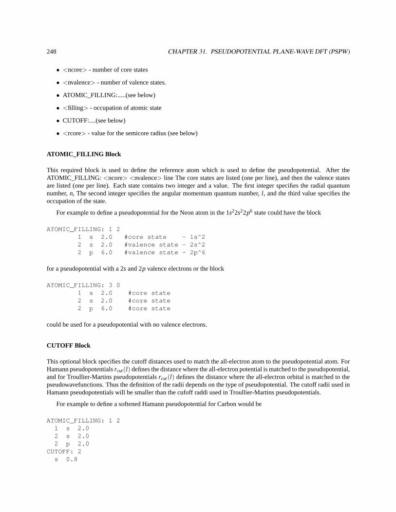
248 CHAPTER 31. PSEUDOPOTENTIAL PLANE-WAVE DFT (PSPW)
• <ncore> - number of core states
• <nvalence> - number of valence states.
• ATOMIC_FILLING:.....(see below)
• <filling> - occupation of atomic state
• CUTOFF:....(see below)
• <rcore> - value for the semicore radius (see below)
ATOMIC_FILLING Block
This required block is used to define the reference atom which is used to define the pseudopotential. After theATOMIC_FILLING: <ncore> <nvalence> line The core states are listed (one per line), and then the valence statesare listed (one per line). Each state contains two integer and a value. The first integer specifies the radial quantumnumber,n, The second integer specifies the angular momentum quantum number,l , and the third value specifies theoccupation of the state.
For example to define a pseudopotential for the Neon atom in the 1s22s22p6 state could have the block
ATOMIC_FILLING: 1 21 s 2.0 #core state - 1s^22 s 2.0 #valence state - 2s^22 p 6.0 #valence state - 2p^6
for a pseudopotential with a 2s and 2p valence electrons or the block
ATOMIC_FILLING: 3 01 s 2.0 #core state2 s 2.0 #core state2 p 6.0 #core state
could be used for a pseudopotential with no valence electrons.
CUTOFF Block
This optional block specifies the cutoff distances used to match the all-electron atom to the pseudopotential atom. ForHamann pseudopotentialsrcut(l) defines the distance where the all-electron potential is matched to the pseudopotential,and for Troullier-Martins pseudopotentialsrcut(l) defines the distance where the all-electron orbital is matched to thepseudowavefunctions. Thus the definition of the radii depends on the type of pseudopotential. The cutoff radii used inHamann pseudopotentials will be smaller than the cufoff raddi used in Troullier-Martins pseudopotentials.
For example to define a softened Hamann pseudopotential for Carbon would be
ATOMIC_FILLING: 1 21 s 2.02 s 2.02 p 2.0
CUTOFF: 2s 0.8
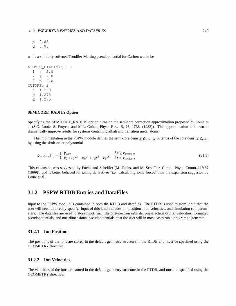
31.2. PSPW RTDB ENTRIES AND DATAFILES 249
p 0.85d 0.85
while a similarly softened Troullier-Marting pseudopotential for Carbon would be
ATOMIC_FILLING: 1 21 s 2.02 s 2.02 p 2.0
CUTOFF: 2s 1.200p 1.275d 1.275
SEMICORE_RADIUS Option
Specifying the SEMICORE_RADIUS option turns on the semicore correction approximation proposed by Louie etal (S.G. Louie, S. Froyen, and M.L. Cohen, Phys. Rev. B,26, 1738, (1982)). This approximation is known todramatically improve results for systems containing alkali and transition metal atoms.
The implmentation in the PSPW module defines the semi-core denisty,ρsemicorein terms of the core density,ρcore,by using the sixth-order polynomial
ρsemicore(r) ={
ρcore if r ≥ rsemicore
c0 +c3r3 +c4r4 +c5r5 +c6r6 if r < rsemicore(31.1)
This expansion was suggested by Fuchs and Scheffler (M. Fuchs, and M. Scheffler, Comp. Phys. Comm.,119,67(1999)), and is better behaved for taking derivatives (i.e. calculating ionic forces) than the expansion suggested byLouie et al.
31.2 PSPW RTDB Entries and DataFiles
Input to the PSPW module is contained in both the RTDB and datafiles. The RTDB is used to store input that theuser will need to directly specify. Input of this kind includes ion positions, ion velocities, and simulation cell param-eters. The datafiles are used to store input, such the one-electron orbitals, one-electron orbital velocities, formattedpseudopotentials, and one-dimensional pseudopotentials, that the user will in most cases run a program to generate.
31.2.1 Ion Positions
The positions of the ions are stored in the default geometry structure in the RTDB and must be specified using theGEOMETRY directive.
31.2.2 Ion Velocities
The velocities of the ions are stored in the default geometry structure in the RTDB, and must be specified using theGEOMETRY directive.
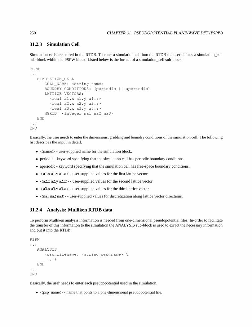
250 CHAPTER 31. PSEUDOPOTENTIAL PLANE-WAVE DFT (PSPW)
31.2.3 Simulation Cell
Simulation cells are stored in the RTDB. To enter a simulation cell into the RTDB the user defines a simulation_cellsub-block within the PSPW block. Listed below is the format of a simulation_cell sub-block.
PSPW...
SIMULATION_CELLCELL_NAME: <string name>BOUNDRY_CONDITIONS: (periodic || aperiodic)LATTICE_VECTORS:
<real a1.x a1.y a1.z><real a2.x a2.y a2.z><real a3.x a3.y a3.z>
NGRID: <integer na1 na2 na3>END
...END
Basically, the user needs to enter the dimensions, gridding and boundry conditions of the simulation cell. The followinglist describes the input in detail.
• <name> - user-supplied name for the simulation block.
• periodic - keyword specifying that the simulation cell has periodic boundary conditions.
• aperiodic - keyword specifying that the simulation cell has free-space boundary conditions.
• <a1.x a1.y a1.z> - user-supplied values for the first lattice vector
• <a2.x a2.y a2.z> - user-supplied values for the second lattice vector
• <a3.x a3.y a3.z> - user-supplied values for the third lattice vector
• <na1 na2 na3> - user-supplied values for discretization along lattice vector directions.
31.2.4 Analysis: Mulliken RTDB data
To perform Mulliken analysis information is needed from one-dimensional pseudopotential files. In-order to facilitatethe transfer of this information to the simulation the ANALYSIS sub-block is used to exract the necessary informationand put it into the RTDB.
PSPW...
ANALYSIS(psp_filename: <string psp_name> \
...)END
...END
Basically, the user needs to enter each pseudopotential used in the simulation.
• <psp_name> - name that ponts to a one-dimensional pseudopotential file.
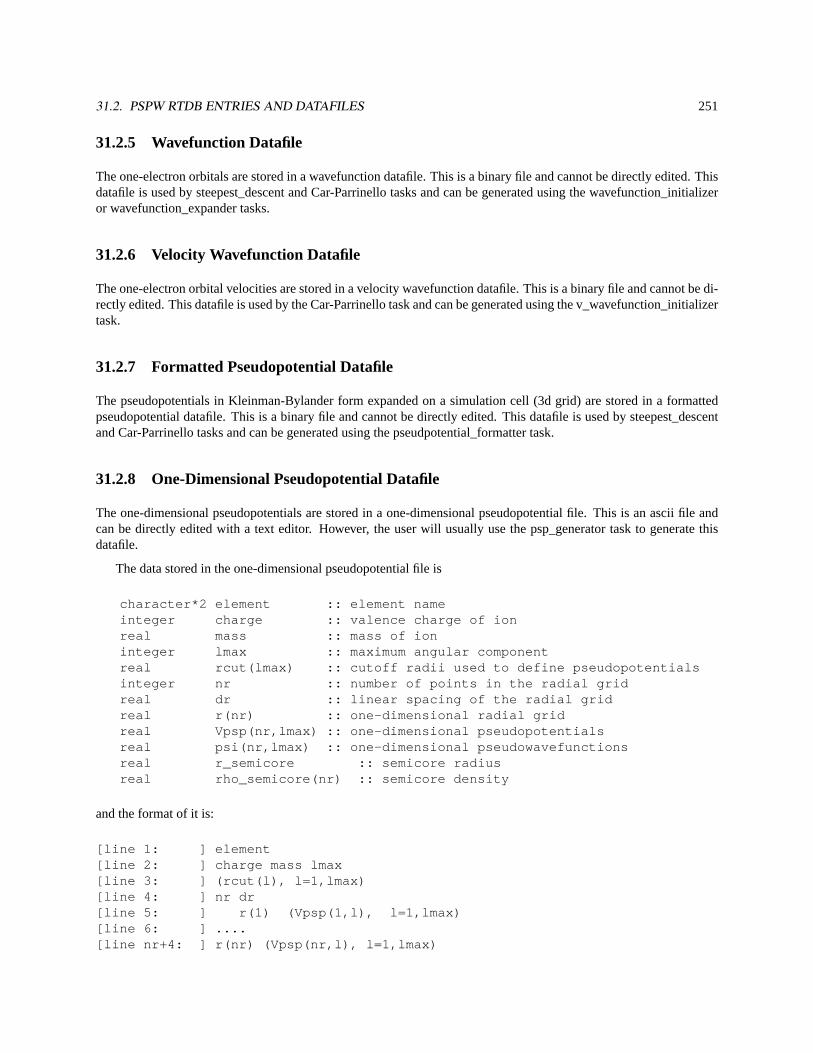
31.2. PSPW RTDB ENTRIES AND DATAFILES 251
31.2.5 Wavefunction Datafile
The one-electron orbitals are stored in a wavefunction datafile. This is a binary file and cannot be directly edited. Thisdatafile is used by steepest_descent and Car-Parrinello tasks and can be generated using the wavefunction_initializeror wavefunction_expander tasks.
31.2.6 Velocity Wavefunction Datafile
The one-electron orbital velocities are stored in a velocity wavefunction datafile. This is a binary file and cannot be di-rectly edited. This datafile is used by the Car-Parrinello task and can be generated using the v_wavefunction_initializertask.
31.2.7 Formatted Pseudopotential Datafile
The pseudopotentials in Kleinman-Bylander form expanded on a simulation cell (3d grid) are stored in a formattedpseudopotential datafile. This is a binary file and cannot be directly edited. This datafile is used by steepest_descentand Car-Parrinello tasks and can be generated using the pseudpotential_formatter task.
31.2.8 One-Dimensional Pseudopotential Datafile
The one-dimensional pseudopotentials are stored in a one-dimensional pseudopotential file. This is an ascii file andcan be directly edited with a text editor. However, the user will usually use the psp_generator task to generate thisdatafile.
The data stored in the one-dimensional pseudopotential file is
character*2 element :: element nameinteger charge :: valence charge of ionreal mass :: mass of ioninteger lmax :: maximum angular componentreal rcut(lmax) :: cutoff radii used to define pseudopotentialsinteger nr :: number of points in the radial gridreal dr :: linear spacing of the radial gridreal r(nr) :: one-dimensional radial gridreal Vpsp(nr,lmax) :: one-dimensional pseudopotentialsreal psi(nr,lmax) :: one-dimensional pseudowavefunctionsreal r_semicore :: semicore radiusreal rho_semicore(nr) :: semicore density
and the format of it is:
[line 1: ] element[line 2: ] charge mass lmax[line 3: ] (rcut(l), l=1,lmax)[line 4: ] nr dr[line 5: ] r(1) (Vpsp(1,l), l=1,lmax)[line 6: ] ....[line nr+4: ] r(nr) (Vpsp(nr,l), l=1,lmax)
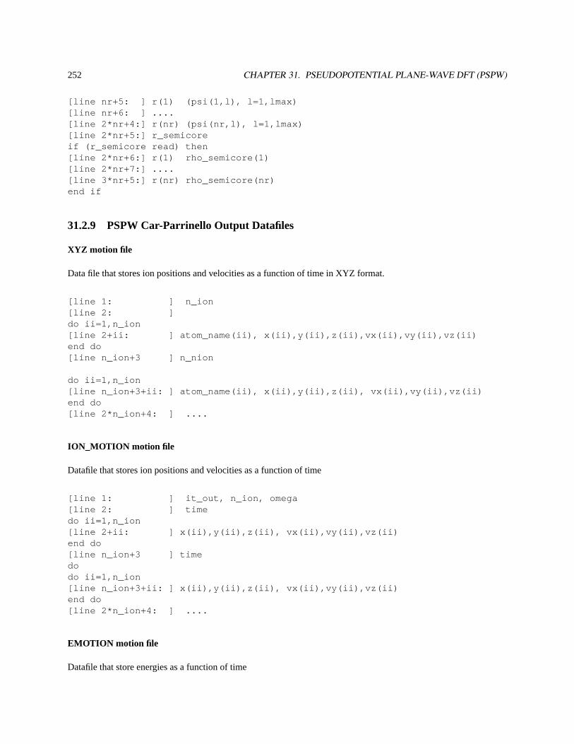
252 CHAPTER 31. PSEUDOPOTENTIAL PLANE-WAVE DFT (PSPW)
[line nr+5: ] r(1) (psi(1,l), l=1,lmax)[line nr+6: ] ....[line 2*nr+4:] r(nr) (psi(nr,l), l=1,lmax)[line 2*nr+5:] r_semicoreif (r_semicore read) then[line 2*nr+6:] r(1) rho_semicore(1)[line 2*nr+7:] ....[line 3*nr+5:] r(nr) rho_semicore(nr)end if
31.2.9 PSPW Car-Parrinello Output Datafiles
XYZ motion file
Data file that stores ion positions and velocities as a function of time in XYZ format.
[line 1: ] n_ion[line 2: ]do ii=1,n_ion[line 2+ii: ] atom_name(ii), x(ii),y(ii),z(ii),vx(ii),vy(ii),vz(ii)end do[line n_ion+3 ] n_nion
do ii=1,n_ion[line n_ion+3+ii: ] atom_name(ii), x(ii),y(ii),z(ii), vx(ii),vy(ii),vz(ii)end do[line 2*n_ion+4: ] ....
ION_MOTION motion file
Datafile that stores ion positions and velocities as a function of time
[line 1: ] it_out, n_ion, omega[line 2: ] timedo ii=1,n_ion[line 2+ii: ] x(ii),y(ii),z(ii), vx(ii),vy(ii),vz(ii)end do[line n_ion+3 ] timedodo ii=1,n_ion[line n_ion+3+ii: ] x(ii),y(ii),z(ii), vx(ii),vy(ii),vz(ii)end do[line 2*n_ion+4: ] ....
EMOTION motion file
Datafile that store energies as a function of time
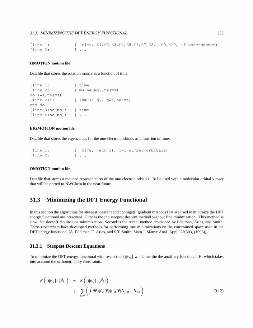
31.3. MINIMIZING THE DFT ENERGY FUNCTIONAL 253
[line 1: ] time, E1,E2,E3,E4,E5,E6,E7,E8, (E9,E10, if Nose-Hoover)[line 2: ] ...
HMOTION motion file
Datafile that stores the rotation matrix as a function of time.
[line 1: ] time[line 2: ] ms,ne(ms),ne(ms)do i=1,ne(ms)[line 2+i: ] (hml(i,j), j=1,ne(ms)end do[line 3+ne(ms): ] time[line 4+ne(ms): ] ....
EIGMOTION motion file
Datafile that stores the eigenvalues for the one-electron orbitals as a function of time.
[line 1: ] time, (eig(i), i=1,number_orbitals)[line 2: ] ...
OMOTION motion file
Datafile that stores a reduced representation of the one-electron orbitals. To be used with a molecular orbital viewerthat will be ported to NWChem in the near future.
31.3 Minimizing the DFT Energy Functional
In this section the algorithms for steepest_descent and conjugate_gradient methods that are used to minimize the DFTenergy functional are presented. First is the the steepest descent method without line minimization. This method isslow, but doesn’t require line minimization. Second is the recent method developed by Edelman, Arias, and Smith.These researchers have developed methods for performing line minimizations on the constrained space used in theDFT energy functional (A. Edelman, T. Arias, and S.T. Smith, Siam J. Matrix Anal. Appl.,20,303, (1998)).
31.3.1 Steepest Descent Equations
To minimize the DFT energy functional with respect to{ψi,σ} we define the the auxiliary functional,F , which takesinto account the orthonormality constraints.
F({ψi,σ},{~RI}
)= E
({ψi,σ},{~RI}
)+ ∑
i j ,σ
(∫d~r ψ∗i,σ(~r)ψ j,σ(~r)Λ ji ,σ−δi j ,σ
)(31.2)
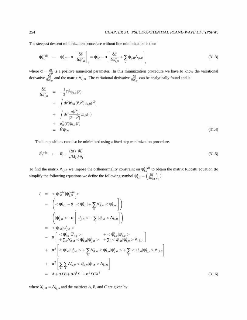
254 CHAPTER 31. PSEUDOPOTENTIAL PLANE-WAVE DFT (PSPW)
The steepest descent minimization procedure without line minimization is then
ψt+∆ti,σ ← ψt
i,σ−α
[δF
δψ∗i,σ
]t
= ψti,σ−α
[δE
δψ∗i,σ+∑
jψ j,σΛ ji ,σ
]t
(31.3)
whereα = ∆t√µ is a positive numerical parameter. In this minimization procedure we have to know the variational
derivative δEδψ∗i,σ
and the matrixΛi j ,σ. The variational derivativeδEδψ∗i,σ
can be analytically found and is
δEδψ∗i,σ
= −12
∇2ψi,σ(~r)
+∫
d~r ′Wext(~r,~r ′)ψi,σ(~r ′)
+∫
d~r ′n(~r ′)
|~r−~r ′|ψi,σ(~r)
+ µσxc(~r)ψi,σ(~r)
≡ Hψi,σ (31.4)
The ion positions can also be minimized using a fixed step minimization procedure.
~Rt+∆tI ← ~Rt
I −(∆t)√
MI
∂E
∂~RI(31.5)
To find the matrixΛi j ,σ we impose the orthonormality constraint onψt+∆ti,σ to obtain the matrix Riccatti equation (to
simplify the following equations we define the following symbolψti,σ =
(δE
δψ∗i,σ
)t
)
I = < ψt+∆ti,σ |ψ
t+∆tj,σ >
=
(< ψt
i,σ|−α
[< ψt
i,σ|+∑k
Λ∗ik,σ < ψtk,σ|
])(|ψt
j,σ >−α
[|ψt
j,σ >+∑l
|ψtl ,σ > Λl j ,σ
])= < ψt
i,σ|ψtj,σ >
− α[< ψt
i,σ|ψtj,σ > +< ψt
i,σ|ψtj,σ >
+∑k Λ∗ik,σ < ψtk,σ|ψt
j,σ > +∑l < ψti,σ|ψt
l ,σ > Λl j ,σ
]+ α2
[< ψt
i,σ|ψtj,σ >+∑
k
Λ∗ik,σ < ψtk,σ|ψt
j,σ >+∑l
< ψti,σ|ψt
l ,σ > Λl j ,σ
]
+ α2
[∑k
∑l
Λ∗ik,σ < ψtk,σ|ψt
l ,σ > Λl j ,σ
]= A+ αXB+ αB†X† + α2XCX† (31.6)
whereXi j ,σ = Λ∗i j ,σ and the matricesA, B, andC are given by
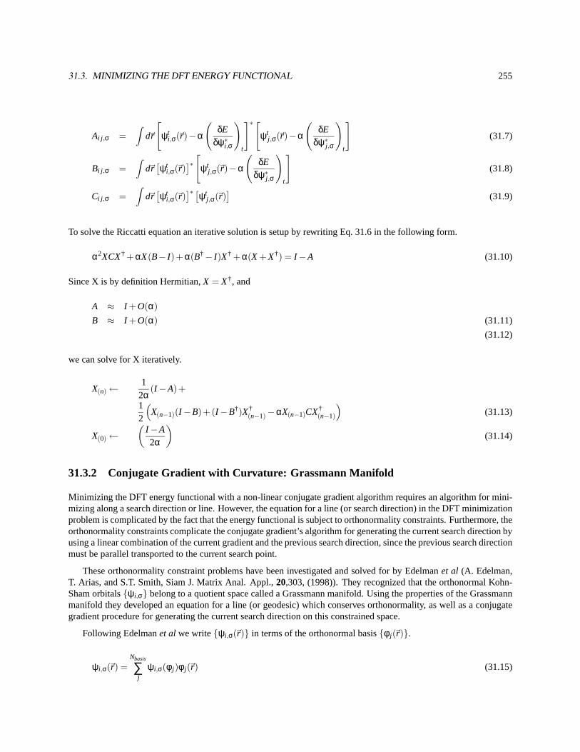
31.3. MINIMIZING THE DFT ENERGY FUNCTIONAL 255
Ai j ,σ =∫
d~r
[ψt
i,σ(~r)−α
(δE
δψ∗i,σ
)t
]∗[ψt
j,σ(~r)−α
(δE
δψ∗j,σ
)t
](31.7)
Bi j ,σ =∫
d~r[ψt
i,σ(~r)]∗[ψt
j,σ(~r)−α
(δE
δψ∗j,σ
)t
](31.8)
Ci j ,σ =∫
d~r[ψt
i,σ(~r)]∗ [ψt
j,σ(~r)]
(31.9)
To solve the Riccatti equation an iterative solution is setup by rewriting Eq. 31.6 in the following form.
α2XCX† + αX(B− I)+ α(B†− I)X† + α(X +X†) = I −A (31.10)
Since X is by definition Hermitian,X = X†, and
A ≈ I +O(α)B ≈ I +O(α) (31.11)
(31.12)
we can solve for X iteratively.
X(n)←1
2α(I −A)+
12
(X(n−1)(I −B)+(I −B†)X†
(n−1)−αX(n−1)CX†(n−1)
)(31.13)
X(0)←(
I −A2α
)(31.14)
31.3.2 Conjugate Gradient with Curvature: Grassmann Manifold
Minimizing the DFT energy functional with a non-linear conjugate gradient algorithm requires an algorithm for mini-mizing along a search direction or line. However, the equation for a line (or search direction) in the DFT minimizationproblem is complicated by the fact that the energy functional is subject to orthonormality constraints. Furthermore, theorthonormality constraints complicate the conjugate gradient’s algorithm for generating the current search direction byusing a linear combination of the current gradient and the previous search direction, since the previous search directionmust be parallel transported to the current search point.
These orthonormality constraint problems have been investigated and solved for by Edelmanet al (A. Edelman,T. Arias, and S.T. Smith, Siam J. Matrix Anal. Appl.,20,303, (1998)). They recognized that the orthonormal Kohn-Sham orbitals{ψi,σ} belong to a quotient space called a Grassmann manifold. Using the properties of the Grassmannmanifold they developed an equation for a line (or geodesic) which conserves orthonormality, as well as a conjugategradient procedure for generating the current search direction on this constrained space.
Following Edelmanet alwe write{ψi,σ(~r)} in terms of the orthonormal basis{φ j(~r)}.
ψi,σ(~r) =Nbasis
∑j
ψi,σ(φ j)φ j(~r) (31.15)
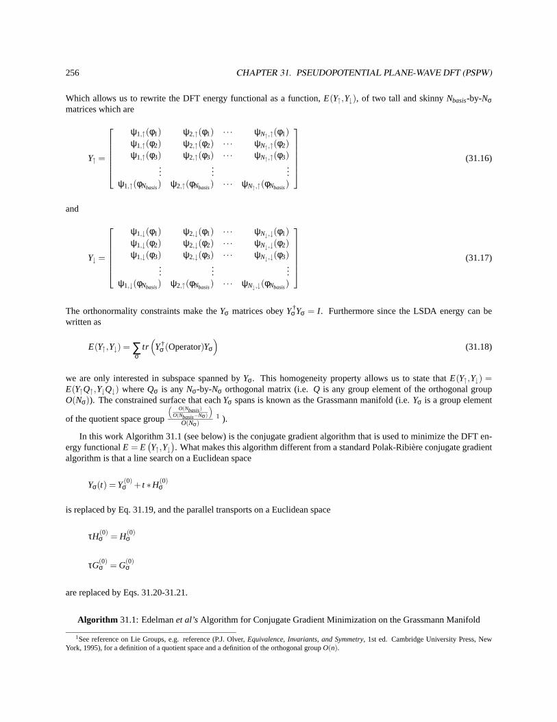
256 CHAPTER 31. PSEUDOPOTENTIAL PLANE-WAVE DFT (PSPW)
Which allows us to rewrite the DFT energy functional as a function,E(Y↑,Y↓), of two tall and skinnyNbasis-by-Nσmatrices which are
Y↑ =
ψ1,↑(φ1) ψ2,↑(φ1) · · · ψN↑,↑(φ1)ψ1,↑(φ2) ψ2,↑(φ2) · · · ψN↑,↑(φ2)ψ1,↑(φ3) ψ2,↑(φ3) · · · ψN↑,↑(φ3)
......
...ψ1,↑(φNbasis) ψ2,↑(φNbasis) · · · ψN↑,↑(φNbasis)
(31.16)
and
Y↓ =
ψ1,↓(φ1) ψ2,↓(φ1) · · · ψN↓,↓(φ1)ψ1,↓(φ2) ψ2,↓(φ2) · · · ψN↓,↓(φ2)ψ1,↓(φ3) ψ2,↓(φ3) · · · ψN↓,↓(φ3)
......
...ψ1,↓(φNbasis) ψ2,↑(φNbasis) · · · ψN↓,↓(φNbasis)
(31.17)
The orthonormality constraints make theYσ matrices obeyY†σYσ = I . Furthermore since the LSDA energy can be
written as
E(Y↑,Y↓) = ∑σ
tr(Y†
σ (Operator)Yσ
)(31.18)
we are only interested in subspace spanned byYσ. This homogeneity property allows us to state thatE(Y↑,Y↓) =E(Y↑Q↑,Y↓Q↓) whereQσ is anyNσ-by-Nσ orthogonal matrix (i.e.Q is any group element of the orthogonal groupO(Nσ)). The constrained surface that eachYσ spans is known as the Grassmann manifold (i.e.Yσ is a group element
of the quotient space group
(O(Nbasis)
O(Nbasis−Nσ)
)O(Nσ)
1 ).
In this work Algorithm 31.1 (see below) is the conjugate gradient algorithm that is used to minimize the DFT en-ergy functionalE = E
(Y↑,Y↓
). What makes this algorithm different from a standard Polak-Ribière conjugate gradient
algorithm is that a line search on a Euclidean space
Yσ(t) = Y(0)σ + t ∗H(0)
σ
is replaced by Eq. 31.19, and the parallel transports on a Euclidean space
τH(0)σ = H(0)
σ
τG(0)σ = G(0)
σ
are replaced by Eqs. 31.20-31.21.
Algorithm 31.1: Edelmanet al’sAlgorithm for Conjugate Gradient Minimization on the Grassmann Manifold
1See reference on Lie Groups, e.g. reference (P.J. Olver,Equivalence, Invariants, and Symmetry, 1st ed. Cambridge University Press, NewYork, 1995), for a definition of a quotient space and a definition of the orthogonal groupO(n).
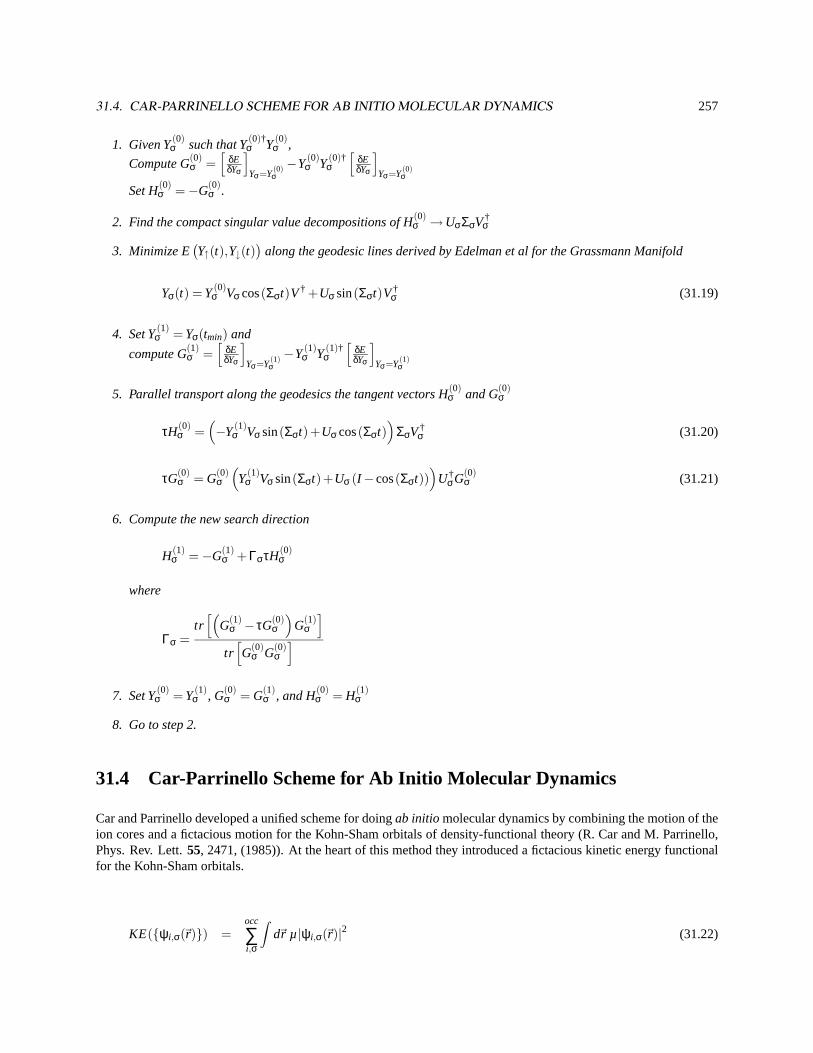
31.4. CAR-PARRINELLO SCHEME FOR AB INITIO MOLECULAR DYNAMICS 257
1. Given Y(0)σ such that Y(0)†
σ Y(0)σ ,
Compute G(0)σ =
[δEδYσ
]Yσ=Y
(0)σ−Y(0)
σ Y(0)†σ
[δEδYσ
]Yσ=Y
(0)σ
Set H(0)σ =−G(0)
σ .
2. Find the compact singular value decompositions of H(0)σ →UσΣσV†
σ
3. Minimize E(Y↑(t),Y↓(t)
)along the geodesic lines derived by Edelman et al for the Grassmann Manifold
Yσ(t) = Y(0)σ Vσ cos(Σσt)V† +Uσ sin(Σσt)V†
σ (31.19)
4. Set Y(1)σ = Yσ(tmin) and
compute G(1)σ =
[δEδYσ
]Yσ=Y
(1)σ−Y(1)
σ Y(1)†σ
[δEδYσ
]Yσ=Y
(1)σ
5. Parallel transport along the geodesics the tangent vectors H(0)σ and G(0)
σ
τH(0)σ =
(−Y(1)
σ Vσ sin(Σσt)+Uσ cos(Σσt))
ΣσV†σ (31.20)
τG(0)σ = G(0)
σ
(Y(1)
σ Vσ sin(Σσt)+Uσ (I −cos(Σσt)))
U†σG(0)
σ (31.21)
6. Compute the new search direction
H(1)σ =−G(1)
σ + ΓστH(0)σ
where
Γσ =tr[(
G(1)σ − τG(0)
σ
)G(1)
σ
]tr[G(0)
σ G(0)σ
]7. Set Y(0)
σ = Y(1)σ , G(0)
σ = G(1)σ , and H(0)
σ = H(1)σ
8. Go to step 2.
31.4 Car-Parrinello Scheme for Ab Initio Molecular Dynamics
Car and Parrinello developed a unified scheme for doingab initio molecular dynamics by combining the motion of theion cores and a fictacious motion for the Kohn-Sham orbitals of density-functional theory (R. Car and M. Parrinello,Phys. Rev. Lett.55, 2471, (1985)). At the heart of this method they introduced a fictacious kinetic energy functionalfor the Kohn-Sham orbitals.
KE({ψi,σ(~r)}) =occ
∑i,σ
∫d~r µ |ψi,σ(~r)|2 (31.22)
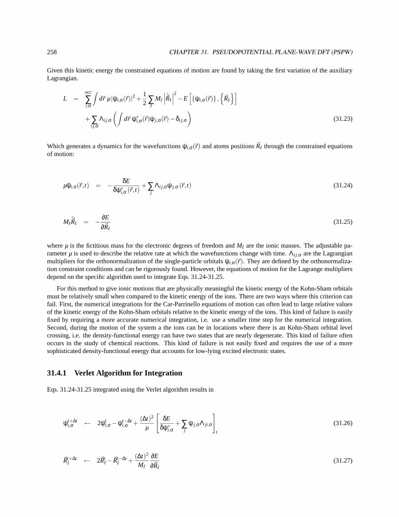
258 CHAPTER 31. PSEUDOPOTENTIAL PLANE-WAVE DFT (PSPW)
Given this kinetic energy the constrained equations of motion are found by taking the first variation of the auxiliaryLagrangian.
L =occ
∑i,σ
∫d~r µ |ψi,σ(~r)|2 +
12 ∑
IMI
∣∣∣~RI
∣∣∣2−E[{ψi,σ(~r)} ,
{~RI
}]+ ∑
i j ,σΛi j ,σ
(∫d~r ψ∗i,σ(~r)ψ j,σ(~r)−δi j ,σ
)(31.23)
Which generates a dynamics for the wavefunctionsψi,σ(~r) and atoms positions~RI through the constrained equationsof motion:
µψi,σ(~r, t) = − δEδψ∗i,σ (~r, t)
+∑j
Λi j ,σψ j,σ (~r, t) (31.24)
MI ~RI = − ∂E
∂~RI(31.25)
whereµ is the fictitious mass for the electronic degrees of freedom andMI are the ionic masses. The adjustable pa-rameterµ is used to describe the relative rate at which the wavefunctions change with time.Λi j ,σ are the Lagrangianmultipliers for the orthonormalization of the single-particle orbitalsψi,σ(~r). They are defined by the orthonormaliza-tion constraint conditions and can be rigorously found. However, the equations of motion for the Lagrange multipliersdepend on the specific algorithm used to integrate Eqs. 31.24-31.25.
For this method to give ionic motions that are physically meaningful the kinetic energy of the Kohn-Sham orbitalsmust be relatively small when compared to the kinetic energy of the ions. There are two ways where this criterion canfail. First, the numerical integrations for the Car-Parrinello equations of motion can often lead to large relative valuesof the kinetic energy of the Kohn-Sham orbitals relative to the kinetic energy of the ions. This kind of failure is easilyfixed by requiring a more accurate numerical integration, i.e. use a smaller time step for the numerical integration.Second, during the motion of the system a the ions can be in locations where there is an Kohn-Sham orbital levelcrossing, i.e. the density-functional energy can have two states that are nearly degenerate. This kind of failure oftenoccurs in the study of chemical reactions. This kind of failure is not easily fixed and requires the use of a moresophisticated density-functional energy that accounts for low-lying excited electronic states.
31.4.1 Verlet Algorithm for Integration
Eqs. 31.24-31.25 integrated using the Verlet algorithm results in
ψt+∆ti,σ ← 2ψt
i,σ−ψt−∆ti,σ +
(∆t)2
µ
[δE
δψ∗i,σ+∑
jψ j,σΛ ji ,σ
]t
(31.26)
~Rt+∆tI ← 2~Rt
I −~Rt−∆tI +
(∆t)2
MI
∂E
∂~RI(31.27)
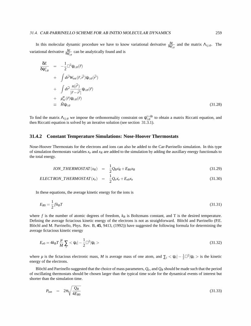
31.4. CAR-PARRINELLO SCHEME FOR AB INITIO MOLECULAR DYNAMICS 259
In this molecular dynamic procedure we have to know variational derivativeδEδψ∗i,σ
and the matrixΛi j ,σ. The
variational derivative δEδψ∗i,σ
can be analytically found and is
δEδψ∗i,σ
= −12
∇2ψi,σ(~r)
+∫
d~r ′Wext(~r,~r ′)ψi,σ(~r ′)
+∫
d~r ′n(~r ′)
|~r−~r ′|ψi,σ(~r)
+ µσxc(~r)ψi,σ(~r)
≡ Hψi,σ (31.28)
To find the matrixΛi j ,σ we impose the orthonormality constraint onψt+∆ti,σ to obtain a matrix Riccatti equation, and
then Riccatti equation is solved by an iterative solution (see section 31.3.1).
31.4.2 Constant Temperature Simulations: Nose-Hoover Thermostats
Nose-Hoover Thermostats for the electrons and ions can also be added to the Car-Parrinello simulation. In this typeof simulation thermostats variablesxe andxR are added to the simulation by adding the auxillary energy functionals tothe total energy.
ION_THERMOSTAT(xR) =12
QRxR+ER0xR (31.29)
ELECTRON_THERMOSTAT(xe) =12
Qexe+Ee0xe (31.30)
In these equations, the average kinetic energy for the ions is
ER0 =12
f kBT (31.31)
where f is the number of atomic degrees of freedom,kB is Boltzmans constant, and T is the desired temperature.Defining the average fictacious kinetic energy of the electrons is not as straighforward. Blöchl and Parrinello (P.E.Blöchl and M. Parrinello, Phys. Rev. B,45, 9413, (1992)) have suggested the following formula for determining theaverage fictacious kinetic energy
Ee0 = 4kBTµM ∑
i< ψi |−
12
∇2|ψi > (31.32)
whereµ is the fictacious electronic mass,M is average mass of one atom, and∑i < ψi | − 12∇2|ψi > is the kinetic
energy of the electrons.
Blöchl and Parrinello suggested that the choice of mass parameters,Qe, andQR should be made such that the periodof oscillating thermostats should be chosen larger than the typical time scale for the dynamical events of interest butshorter than the simulation time.
Pion = 2π√
QR
4ER0(31.33)
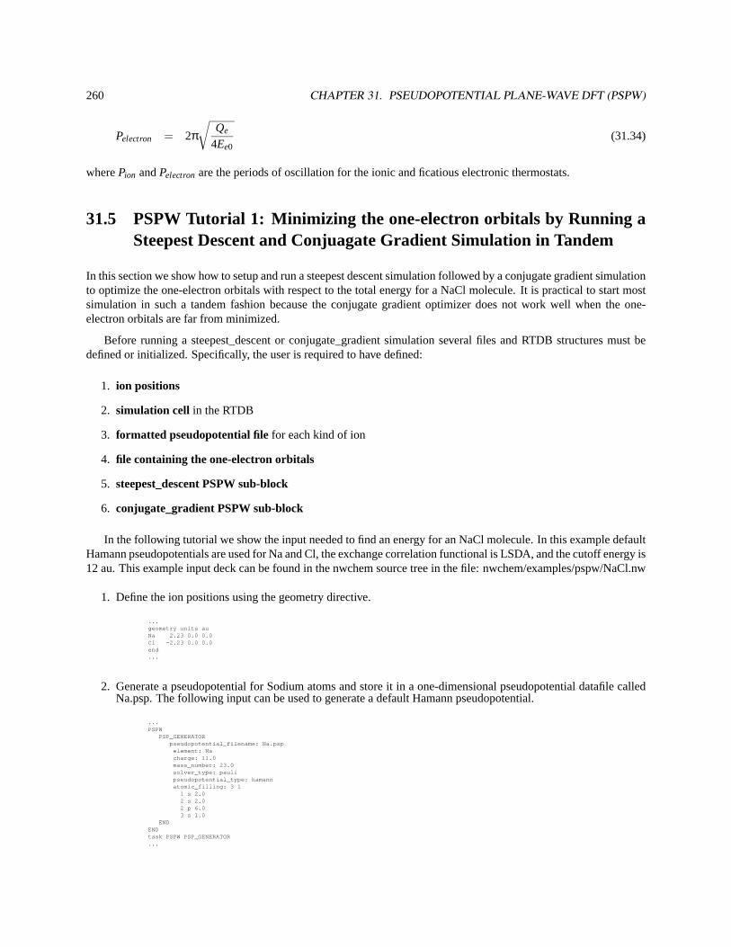
260 CHAPTER 31. PSEUDOPOTENTIAL PLANE-WAVE DFT (PSPW)
Pelectron = 2π√
Qe
4Ee0(31.34)
wherePion andPelectronare the periods of oscillation for the ionic and ficatious electronic thermostats.
31.5 PSPW Tutorial 1: Minimizing the one-electron orbitals by Running aSteepest Descent and Conjuagate Gradient Simulation in Tandem
In this section we show how to setup and run a steepest descent simulation followed by a conjugate gradient simulationto optimize the one-electron orbitals with respect to the total energy for a NaCl molecule. It is practical to start mostsimulation in such a tandem fashion because the conjugate gradient optimizer does not work well when the one-electron orbitals are far from minimized.
Before running a steepest_descent or conjugate_gradient simulation several files and RTDB structures must bedefined or initialized. Specifically, the user is required to have defined:
1. ion positions
2. simulation cell in the RTDB
3. formatted pseudopotential filefor each kind of ion
4. file containing the one-electron orbitals
5. steepest_descent PSPW sub-block
6. conjugate_gradient PSPW sub-block
In the following tutorial we show the input needed to find an energy for an NaCl molecule. In this example defaultHamann pseudopotentials are used for Na and Cl, the exchange correlation functional is LSDA, and the cutoff energy is12 au. This example input deck can be found in the nwchem source tree in the file: nwchem/examples/pspw/NaCl.nw
1. Define the ion positions using the geometry directive.
...geometry units auNa 2.23 0.0 0.0Cl -2.23 0.0 0.0end...
2. Generate a pseudopotential for Sodium atoms and store it in a one-dimensional pseudopotential datafile calledNa.psp. The following input can be used to generate a default Hamann pseudopotential.
...PSPW
PSP_GENERATORpseudopotential_filename: Na.psp
element: Nacharge: 11.0mass_number: 23.0solver_type: paulipseudopotential_type: hamannatomic_filling: 3 1
1 s 2.02 s 2.02 p 6.03 s 1.0
ENDENDtask PSPW PSP_GENERATOR...
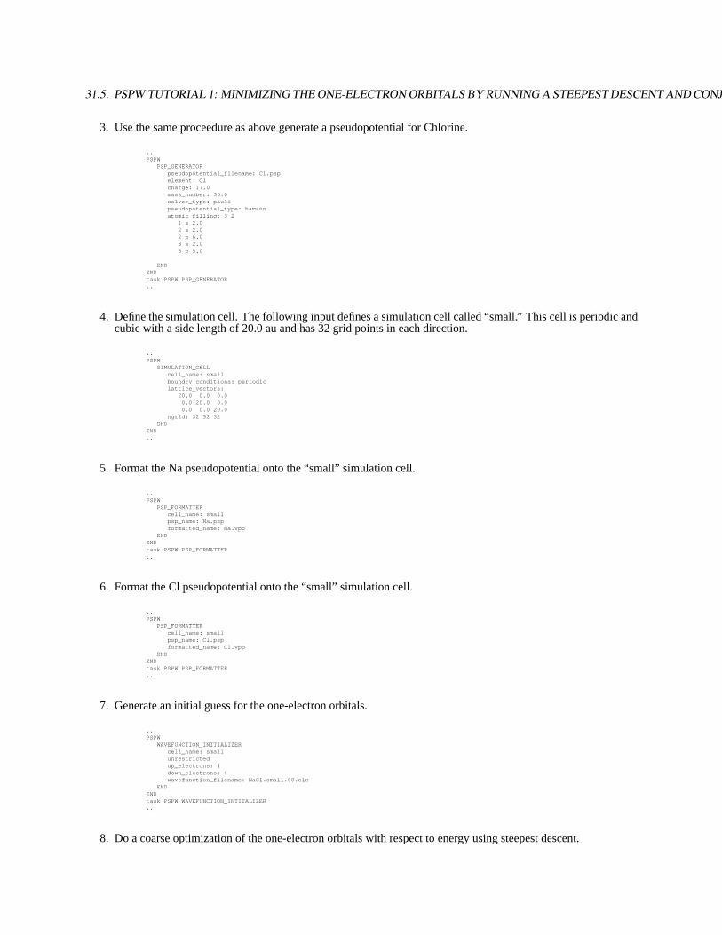
31.5. PSPW TUTORIAL 1: MINIMIZING THE ONE-ELECTRON ORBITALS BY RUNNING A STEEPEST DESCENT AND CONJUAGATE GRADIENT SIMULATION IN TANDEM261
3. Use the same proceedure as above generate a pseudopotential for Chlorine.
...PSPW
PSP_GENERATORpseudopotential_filename: Cl.pspelement: Clcharge: 17.0mass_number: 35.0solver_type: paulipseudopotential_type: hamannatomic_filling: 3 2
1 s 2.02 s 2.02 p 6.03 s 2.03 p 5.0
ENDENDtask PSPW PSP_GENERATOR...
4. Define the simulation cell. The following input defines a simulation cell called “small.” This cell is periodic andcubic with a side length of 20.0 au and has 32 grid points in each direction.
...PSPW
SIMULATION_CELLcell_name: smallboundry_conditions: periodiclattice_vectors:
20.0 0.0 0.00.0 20.0 0.00.0 0.0 20.0
ngrid: 32 32 32END
END...
5. Format the Na pseudopotential onto the “small” simulation cell.
...PSPW
PSP_FORMATTERcell_name: smallpsp_name: Na.pspformatted_name: Na.vpp
ENDENDtask PSPW PSP_FORMATTER...
6. Format the Cl pseudopotential onto the “small” simulation cell.
...PSPW
PSP_FORMATTERcell_name: smallpsp_name: Cl.pspformatted_name: Cl.vpp
ENDENDtask PSPW PSP_FORMATTER...
7. Generate an initial guess for the one-electron orbitals.
...PSPW
WAVEFUNCTION_INITIALIZERcell_name: smallunrestrictedup_electrons: 4down_electrons: 4wavefunction_filename: NaCl.small.00.elc
ENDENDtask PSPW WAVEFUNCTION_INTITALIZER...
8. Do a coarse optimization of the one-electron orbitals with respect to energy using steepest descent.
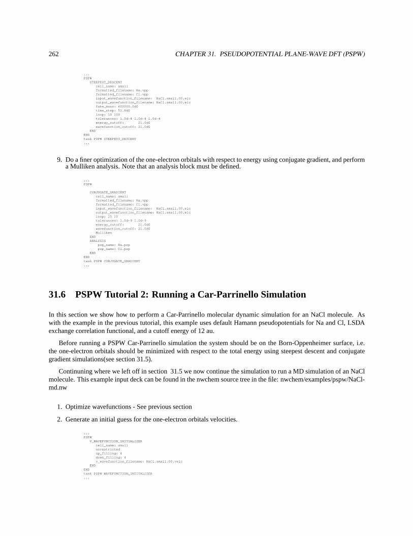
262 CHAPTER 31. PSEUDOPOTENTIAL PLANE-WAVE DFT (PSPW)
...PSPW
STEEPEST_DESCENTcell_name: smallformatted_filename: Na.vppformatted_filename: Cl.vppinput_wavefunction_filename: NaCl.small.00.elcoutput_wavefunction_filename: NaCl.small.00.elcfake_mass: 400000.0d0time_step: 51.8d0loop: 10 100tolerances: 1.0d-4 1.0d-4 1.0d-4energy_cutoff: 21.0d0wavefunction_cutoff: 21.0d0
ENDENDtask PSPW STEEPEST_DESCENT...
9. Do a finer optimization of the one-electron orbitals with respect to energy using conjugate gradient, and performa Mulliken analysis. Note that an analysis block must be defined.
...PSPW
CONJUGATE_GRADIENTcell_name: smallformatted_filename: Na.vppformatted_filename: Cl.vppinput_wavefunction_filename: NaCl.small.00.elcoutput_wavefunction_filename: NaCl.small.00.elcloop: 25 10tolerances: 1.0d-9 1.0d-9energy_cutoff: 21.0d0wavefunction_cutoff: 21.0d0Mulliken
ENDANALYSIS
psp_name: Na.psppsp_name: Cl.psp
ENDENDtask PSPW CONJUGATE_GRADIENT...
31.6 PSPW Tutorial 2: Running a Car-Parrinello Simulation
In this section we show how to perform a Car-Parrinello molecular dynamic simulation for an NaCl molecule. Aswith the example in the previous tutorial, this example uses default Hamann pseudopotentials for Na and Cl, LSDAexchange correlation functional, and a cutoff energy of 12 au.
Before running a PSPW Car-Parrinello simulation the system should be on the Born-Oppenheimer surface, i.e.the one-electron orbitals should be minimized with respect to the total energy using steepest descent and conjugategradient simulations(see section 31.5).
Continuning where we left off in section 31.5 we now continue the simulation to run a MD simulation of an NaClmolecule. This example input deck can be found in the nwchem source tree in the file: nwchem/examples/pspw/NaCl-md.nw
1. Optimize wavefunctions - See previous section
2. Generate an initial guess for the one-electron orbitals velocities.
...PSPW
V_WAVEFUNCTION_INITIALIZERcell_name: smallunrestrictedup_filling: 4down_filling: 4v_wavefunction_filename: NaCl.small.00.velc
ENDENDtask PSPW WAVEFUNCTION_INTITALIZER...
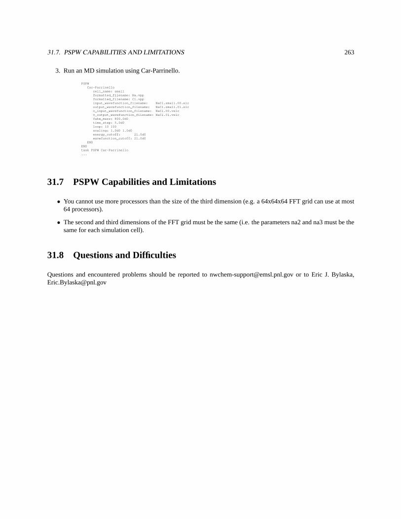
31.7. PSPW CAPABILITIES AND LIMITATIONS 263
3. Run an MD simulation using Car-Parrinello.
PSPWCar-Parrinello
cell_name: smallformatted_filename: Na.vppformatted_filename: Cl.vppinput_wavefunction_filename: NaCl.small.00.elcoutput_wavefunction_filename: NaCl.small.01.elcv_input_wavefunction_filename: NaCl.00.velcv_output_wavefunction_filename: NaCl.01.velcfake_mass: 800.0d0time_step: 5.0d0loop: 10 100scaling: 1.0d0 1.0d0energy_cutoff: 21.0d0wavefunction_cutoff: 21.0d0
ENDENDtask PSPW Car-Parrinello...
31.7 PSPW Capabilities and Limitations
• You cannot use more processors than the size of the third dimension (e.g. a 64x64x64 FFT grid can use at most64 processors).
• The second and third dimensions of the FFT grid must be the same (i.e. the parameters na2 and na3 must be thesame for each simulation cell).
31.8 Questions and Difficulties
Questions and encountered problems should be reported to [email protected] or to Eric J. Bylaska,[email protected]

264 CHAPTER 31. PSEUDOPOTENTIAL PLANE-WAVE DFT (PSPW)
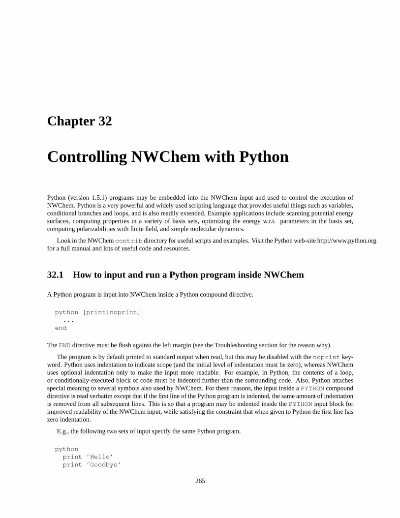
Chapter 32
Controlling NWChem with Python
Python (version 1.5.1) programs may be embedded into the NWChem input and used to control the execution ofNWChem. Python is a very powerful and widely used scripting language that provides useful things such as variables,conditional branches and loops, and is also readily extended. Example applications include scanning potential energysurfaces, computing properties in a variety of basis sets, optimizing the energy w.r.t. parameters in the basis set,computing polarizabilities with finite field, and simple molecular dynamics.
Look in the NWChemcontrib directory for useful scripts and examples. Visit the Python web-site http://www.python.orgfor a full manual and lots of useful code and resources.
32.1 How to input and run a Python program inside NWChem
A Python program is input into NWChem inside a Python compound directive.
python [print|noprint]...
end
TheENDdirective must be flush against the left margin (see the Troubleshooting section for the reason why).
The program is by default printed to standard output when read, but this may be disabled with thenoprint key-word. Python uses indentation to indicate scope (and the initial level of indentation must be zero), whereas NWChemuses optional indentation only to make the input more readable. For example, in Python, the contents of a loop,or conditionally-executed block of code must be indented further than the surrounding code. Also, Python attachesspecial meaning to several symbols also used by NWChem. For these reasons, the input inside aPYTHONcompounddirective is read verbatim except that if the first line of the Python program is indented, the same amount of indentationis removed from all subsequent lines. This is so that a program may be indented inside thePYTHONinput block forimproved readability of the NWChem input, while satisfying the constraint that when given to Python the first line haszero indentation.
E.g., the following two sets of input specify the same Python program.
pythonprint ’Hello’print ’Goodbye’
265
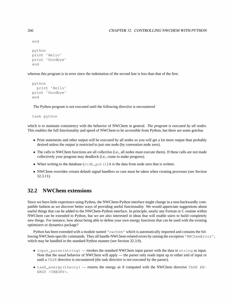
266 CHAPTER 32. CONTROLLING NWCHEM WITH PYTHON
end
pythonprint ’Hello’print ’Goodbye’end
whereas this program is in error since the indentation of the second line is less than that of the first.
pythonprint ’Hello’
print ’Goodbye’end
The Python program is not executed until the following directive is encountered
task python
which is to maintain consistency with the behavior of NWChem in general.The program is executed by all nodes.This enables the full functionality and speed of NWChem to be accessible from Python, but there are some gotchas
• Print statements and other output will be executed by all nodes so you will get a lot more output than probablydesired unless the output is restricted to just one node (by convention node zero).
• The calls to NWChem functions are all collective (i.e., all nodes must execute them). If these calls are not madecollectively your program may deadlock (i.e., cease to make progress).
• When writing to the database (rtdb_put() ) it is the data from node zero that is written.
• NWChem overrides certain default signal handlers so care must be taken when creating processes (see Section32.3.11).
32.2 NWChem extensions
Since we have little experience using Python, the NWChem-Python interface might change in a non-backwardly com-patible fashion as we discover better ways of providing useful functionality. We would appreciate suggestions aboutuseful things that can be added to the NWChem-Python interface. In principle, nearly any Fortran or C routine withinNWChem can be extended to Python, but we are also interested in ideas that will enable users to build completelynew things. For instance, how about being able to define your own energy functions that can be used with the existingoptimizers or dynamics package?
Python has been extended with a module named"nwchem" which is automatically imported and contains the fol-lowing NWChem-specific commands. They all handle NWChem-related errors by raising the exception"NWChemError" ,which may be handled in the standard Python manner (see Section 32.3.9).
• input_parse(string) — invokes the standard NWChem input parser with the data instring as input.Note that the usual behavior of NWChem will apply — the parser only reads input up to either end of input oruntil aTASKdirective is encountered (the task directive isnotexecuted by the parser).
• task_energy(theory) — returns the energy as if computed with the NWChem directiveTASK EN-ERGY <THEORY>.
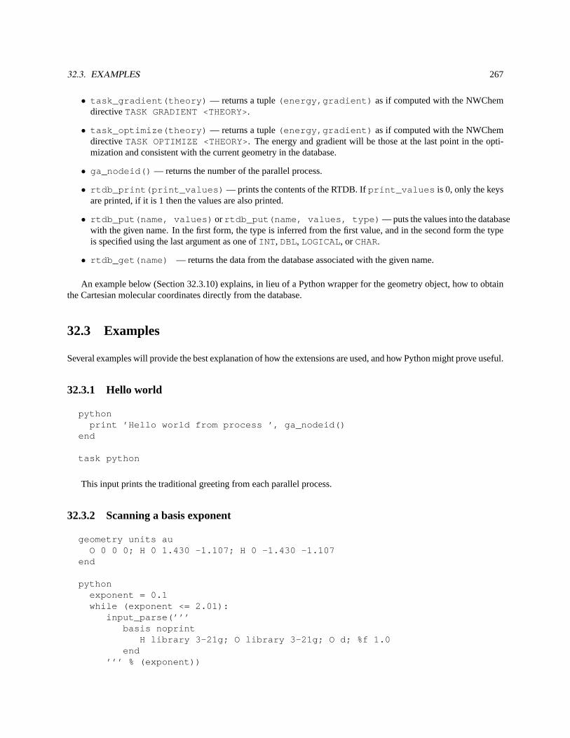
32.3. EXAMPLES 267
• task_gradient(theory) — returns a tuple(energy,gradient) as if computed with the NWChemdirectiveTASK GRADIENT <THEORY>.
• task_optimize(theory) — returns a tuple(energy,gradient) as if computed with the NWChemdirectiveTASK OPTIMIZE <THEORY>. The energy and gradient will be those at the last point in the opti-mization and consistent with the current geometry in the database.
• ga_nodeid() — returns the number of the parallel process.
• rtdb_print(print_values) — prints the contents of the RTDB. Ifprint_values is 0, only the keysare printed, if it is 1 then the values are also printed.
• rtdb_put(name, values) or rtdb_put(name, values, type) — puts the values into the databasewith the given name. In the first form, the type is inferred from the first value, and in the second form the typeis specified using the last argument as one ofINT , DBL, LOGICAL, or CHAR.
• rtdb_get(name) — returns the data from the database associated with the given name.
An example below (Section 32.3.10) explains, in lieu of a Python wrapper for the geometry object, how to obtainthe Cartesian molecular coordinates directly from the database.
32.3 Examples
Several examples will provide the best explanation of how the extensions are used, and how Python might prove useful.
32.3.1 Hello world
pythonprint ’Hello world from process ’, ga_nodeid()
end
task python
This input prints the traditional greeting from each parallel process.
32.3.2 Scanning a basis exponent
geometry units auO 0 0 0; H 0 1.430 -1.107; H 0 -1.430 -1.107
end
pythonexponent = 0.1while (exponent <= 2.01):
input_parse(’’’basis noprint
H library 3-21g; O library 3-21g; O d; %f 1.0end
’’’ % (exponent))
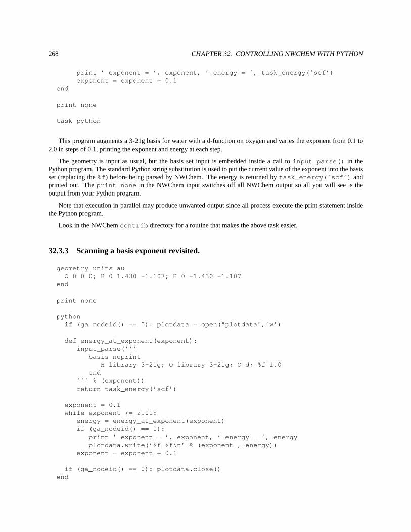
268 CHAPTER 32. CONTROLLING NWCHEM WITH PYTHON
print ’ exponent = ’, exponent, ’ energy = ’, task_energy(’scf’)exponent = exponent + 0.1
end
print none
task python
This program augments a 3-21g basis for water with a d-function on oxygen and varies the exponent from 0.1 to2.0 in steps of 0.1, printing the exponent and energy at each step.
The geometry is input as usual, but the basis set input is embedded inside a call toinput_parse() in thePython program. The standard Python string substitution is used to put the current value of the exponent into the basisset (replacing the%f) before being parsed by NWChem. The energy is returned bytask_energy(’scf’) andprinted out. Theprint none in the NWChem input switches off all NWChem output so all you will see is theoutput from your Python program.
Note that execution in parallel may produce unwanted output since all process execute the print statement insidethe Python program.
Look in the NWChemcontrib directory for a routine that makes the above task easier.
32.3.3 Scanning a basis exponent revisited.
geometry units auO 0 0 0; H 0 1.430 -1.107; H 0 -1.430 -1.107
end
print none
pythonif (ga_nodeid() == 0): plotdata = open("plotdata",’w’)
def energy_at_exponent(exponent):input_parse(’’’
basis noprintH library 3-21g; O library 3-21g; O d; %f 1.0
end’’’ % (exponent))return task_energy(’scf’)
exponent = 0.1while exponent <= 2.01:
energy = energy_at_exponent(exponent)if (ga_nodeid() == 0):
print ’ exponent = ’, exponent, ’ energy = ’, energyplotdata.write(’%f %f\n’ % (exponent , energy))
exponent = exponent + 0.1
if (ga_nodeid() == 0): plotdata.close()end
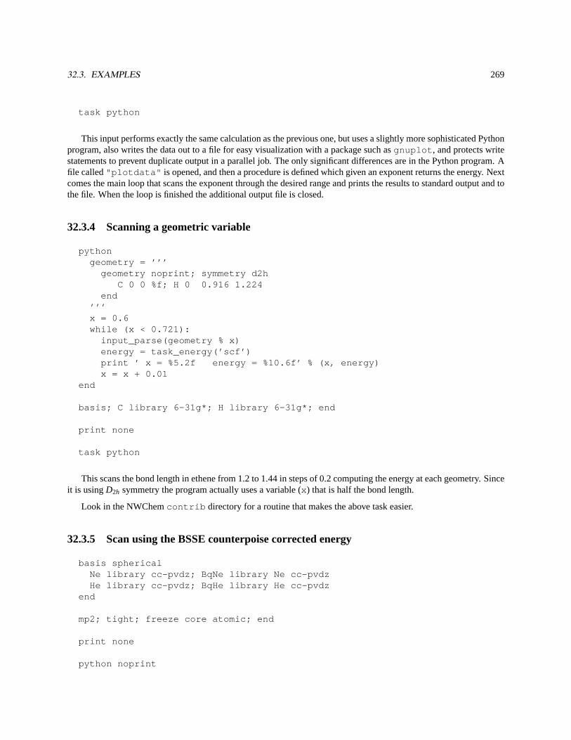
32.3. EXAMPLES 269
task python
This input performs exactly the same calculation as the previous one, but uses a slightly more sophisticated Pythonprogram, also writes the data out to a file for easy visualization with a package such asgnuplot , and protects writestatements to prevent duplicate output in a parallel job. The only significant differences are in the Python program. Afile called"plotdata" is opened, and then a procedure is defined which given an exponent returns the energy. Nextcomes the main loop that scans the exponent through the desired range and prints the results to standard output and tothe file. When the loop is finished the additional output file is closed.
32.3.4 Scanning a geometric variable
pythongeometry = ’’’
geometry noprint; symmetry d2hC 0 0 %f; H 0 0.916 1.224
end’’’x = 0.6while (x < 0.721):
input_parse(geometry % x)energy = task_energy(’scf’)print ’ x = %5.2f energy = %10.6f’ % (x, energy)x = x + 0.01
end
basis; C library 6-31g*; H library 6-31g*; end
print none
task python
This scans the bond length in ethene from 1.2 to 1.44 in steps of 0.2 computing the energy at each geometry. Sinceit is usingD2h symmetry the program actually uses a variable (x ) that is half the bond length.
Look in the NWChemcontrib directory for a routine that makes the above task easier.
32.3.5 Scan using the BSSE counterpoise corrected energy
basis sphericalNe library cc-pvdz; BqNe library Ne cc-pvdzHe library cc-pvdz; BqHe library He cc-pvdz
end
mp2; tight; freeze core atomic; end
print none
python noprint
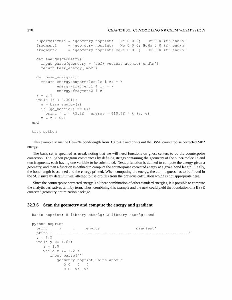
270 CHAPTER 32. CONTROLLING NWCHEM WITH PYTHON
supermolecule = ’geometry noprint; Ne 0 0 0; He 0 0 %f; end\n’fragment1 = ’geometry noprint; Ne 0 0 0; BqHe 0 0 %f; end\n’fragment2 = ’geometry noprint; BqNe 0 0 0; He 0 0 %f; end\n’
def energy(geometry):input_parse(geometry + ’scf; vectors atomic; end\n’)return task_energy(’mp2’)
def bsse_energy(z):return energy(supermolecule % z) - \
energy(fragment1 % z) - \energy(fragment2 % z)
z = 3.3while (z < 4.301):
e = bsse_energy(z)if (ga_nodeid() == 0):
print ’ z = %5.2f energy = %10.7f ’ % (z, e)z = z + 0.1
end
task python
This example scans the He—Ne bond-length from 3.3 to 4.3 and prints out the BSSE counterpoise corrected MP2energy.
The basis set is specified as usual, noting that we will need functions on ghost centers to do the counterpoisecorrection. The Python program commences by defining strings containing the geometry of the super-molecule andtwo fragments, each having one variable to be substituted. Next, a function is defined to compute the energy given ageometry, and then a function is defined to compute the counterpoise corrected energy at a given bond length. Finally,the bond length is scanned and the energy printed. When computing the energy, the atomic guess has to be forced inthe SCF since by default it will attempt to use orbitals from the previous calculation which is not appropriate here.
Since the counterpoise corrected energy is a linear combination of other standard energies, it is possible to computethe analytic derivatives term by term. Thus, combining this example and the next could yield the foundation of a BSSEcorrected geometry optimization package.
32.3.6 Scan the geometry and compute the energy and gradient
basis noprint; H library sto-3g; O library sto-3g; end
python noprintprint ’ y z energy gradient’print ’ ----- ----- ---------- ------------------------------------’y = 1.2while y <= 1.61:
z = 1.0while z <= 1.21:
input_parse(’’’geometry noprint units atomic
O 0 0 0H 0 %f -%f
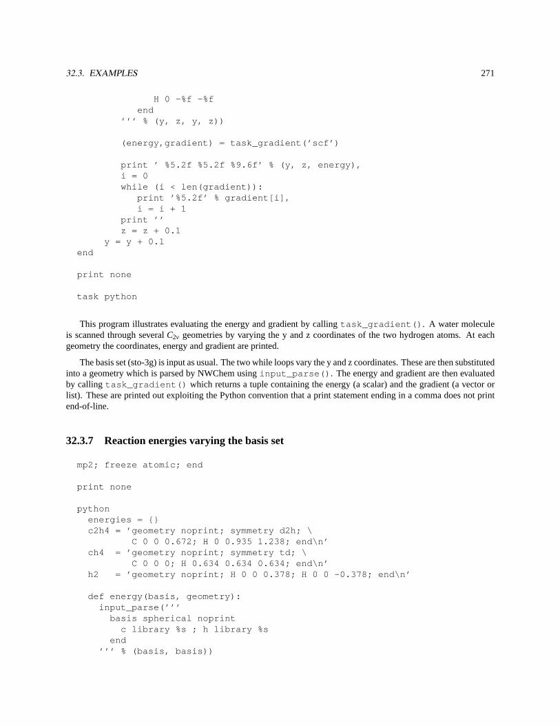
32.3. EXAMPLES 271
H 0 -%f -%fend
’’’ % (y, z, y, z))
(energy,gradient) = task_gradient(’scf’)
print ’ %5.2f %5.2f %9.6f’ % (y, z, energy),i = 0while (i < len(gradient)):
print ’%5.2f’ % gradient[i],i = i + 1
print ’’z = z + 0.1
y = y + 0.1end
print none
task python
This program illustrates evaluating the energy and gradient by callingtask_gradient() . A water moleculeis scanned through severalC2v geometries by varying the y and z coordinates of the two hydrogen atoms. At eachgeometry the coordinates, energy and gradient are printed.
The basis set (sto-3g) is input as usual. The two while loops vary the y and z coordinates. These are then substitutedinto a geometry which is parsed by NWChem usinginput_parse() . The energy and gradient are then evaluatedby calling task_gradient() which returns a tuple containing the energy (a scalar) and the gradient (a vector orlist). These are printed out exploiting the Python convention that a print statement ending in a comma does not printend-of-line.
32.3.7 Reaction energies varying the basis set
mp2; freeze atomic; end
print none
pythonenergies = {}c2h4 = ’geometry noprint; symmetry d2h; \
C 0 0 0.672; H 0 0.935 1.238; end\n’ch4 = ’geometry noprint; symmetry td; \
C 0 0 0; H 0.634 0.634 0.634; end\n’h2 = ’geometry noprint; H 0 0 0.378; H 0 0 -0.378; end\n’
def energy(basis, geometry):input_parse(’’’
basis spherical noprintc library %s ; h library %s
end’’’ % (basis, basis))
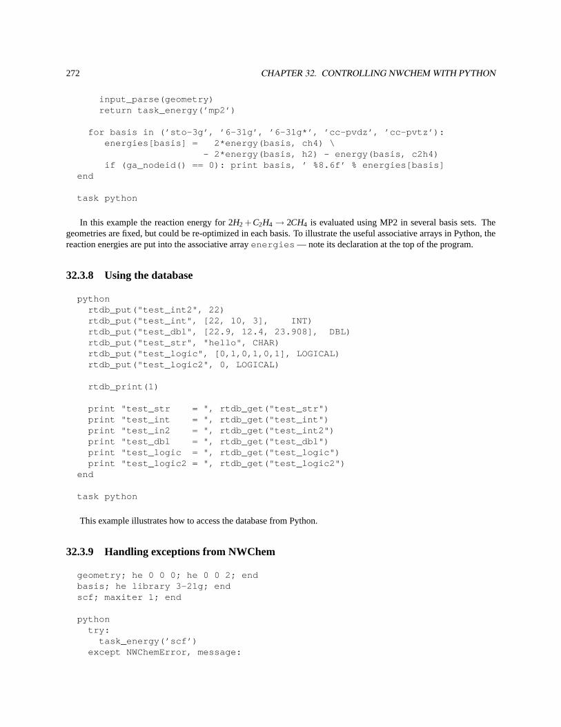
272 CHAPTER 32. CONTROLLING NWCHEM WITH PYTHON
input_parse(geometry)return task_energy(’mp2’)
for basis in (’sto-3g’, ’6-31g’, ’6-31g*’, ’cc-pvdz’, ’cc-pvtz’):energies[basis] = 2*energy(basis, ch4) \
- 2*energy(basis, h2) - energy(basis, c2h4)if (ga_nodeid() == 0): print basis, ’ %8.6f’ % energies[basis]
end
task python
In this example the reaction energy for 2H2 +C2H4→ 2CH4 is evaluated using MP2 in several basis sets. Thegeometries are fixed, but could be re-optimized in each basis. To illustrate the useful associative arrays in Python, thereaction energies are put into the associative arrayenergies — note its declaration at the top of the program.
32.3.8 Using the database
pythonrtdb_put("test_int2", 22)rtdb_put("test_int", [22, 10, 3], INT)rtdb_put("test_dbl", [22.9, 12.4, 23.908], DBL)rtdb_put("test_str", "hello", CHAR)rtdb_put("test_logic", [0,1,0,1,0,1], LOGICAL)rtdb_put("test_logic2", 0, LOGICAL)
rtdb_print(1)
print "test_str = ", rtdb_get("test_str")print "test_int = ", rtdb_get("test_int")print "test_in2 = ", rtdb_get("test_int2")print "test_dbl = ", rtdb_get("test_dbl")print "test_logic = ", rtdb_get("test_logic")print "test_logic2 = ", rtdb_get("test_logic2")
end
task python
This example illustrates how to access the database from Python.
32.3.9 Handling exceptions from NWChem
geometry; he 0 0 0; he 0 0 2; endbasis; he library 3-21g; endscf; maxiter 1; end
pythontry:
task_energy(’scf’)except NWChemError, message:
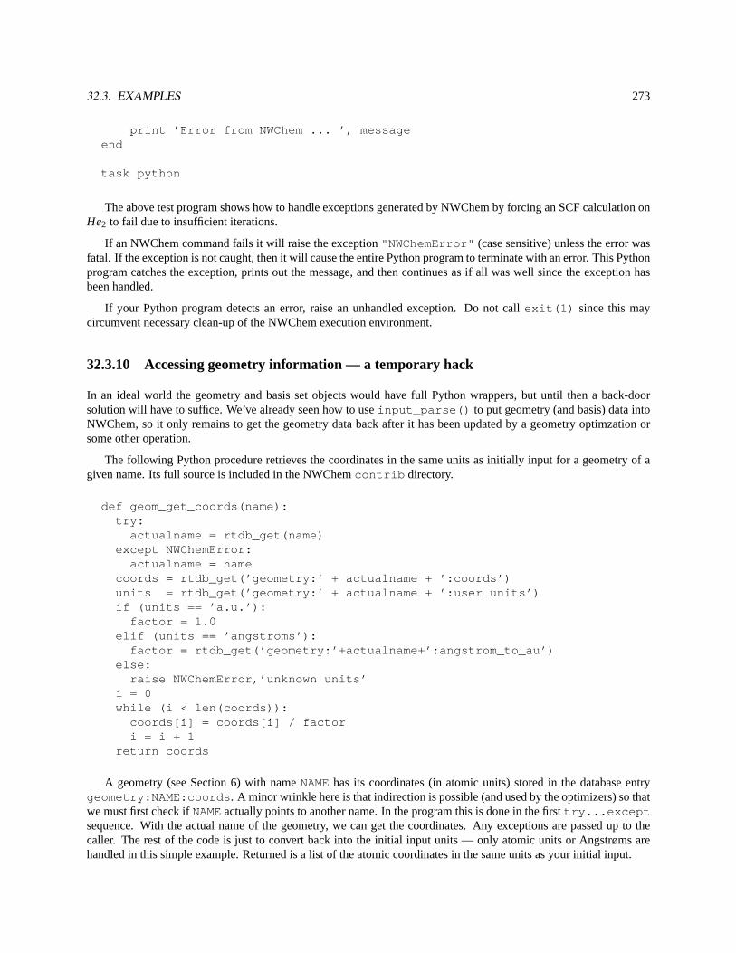
32.3. EXAMPLES 273
print ’Error from NWChem ... ’, messageend
task python
The above test program shows how to handle exceptions generated by NWChem by forcing an SCF calculation onHe2 to fail due to insufficient iterations.
If an NWChem command fails it will raise the exception"NWChemError" (case sensitive) unless the error wasfatal. If the exception is not caught, then it will cause the entire Python program to terminate with an error. This Pythonprogram catches the exception, prints out the message, and then continues as if all was well since the exception hasbeen handled.
If your Python program detects an error, raise an unhandled exception. Do not callexit(1) since this maycircumvent necessary clean-up of the NWChem execution environment.
32.3.10 Accessing geometry information — a temporary hack
In an ideal world the geometry and basis set objects would have full Python wrappers, but until then a back-doorsolution will have to suffice. We’ve already seen how to useinput_parse() to put geometry (and basis) data intoNWChem, so it only remains to get the geometry data back after it has been updated by a geometry optimzation orsome other operation.
The following Python procedure retrieves the coordinates in the same units as initially input for a geometry of agiven name. Its full source is included in the NWChemcontrib directory.
def geom_get_coords(name):try:
actualname = rtdb_get(name)except NWChemError:
actualname = namecoords = rtdb_get(’geometry:’ + actualname + ’:coords’)units = rtdb_get(’geometry:’ + actualname + ’:user units’)if (units == ’a.u.’):
factor = 1.0elif (units == ’angstroms’):
factor = rtdb_get(’geometry:’+actualname+’:angstrom_to_au’)else:
raise NWChemError,’unknown units’i = 0while (i < len(coords)):
coords[i] = coords[i] / factori = i + 1
return coords
A geometry (see Section 6) with nameNAMEhas its coordinates (in atomic units) stored in the database entrygeometry:NAME:coords . A minor wrinkle here is that indirection is possible (and used by the optimizers) so thatwe must first check ifNAMEactually points to another name. In the program this is done in the firsttry...exceptsequence. With the actual name of the geometry, we can get the coordinates. Any exceptions are passed up to thecaller. The rest of the code is just to convert back into the initial input units — only atomic units or Angstrøms arehandled in this simple example. Returned is a list of the atomic coordinates in the same units as your initial input.
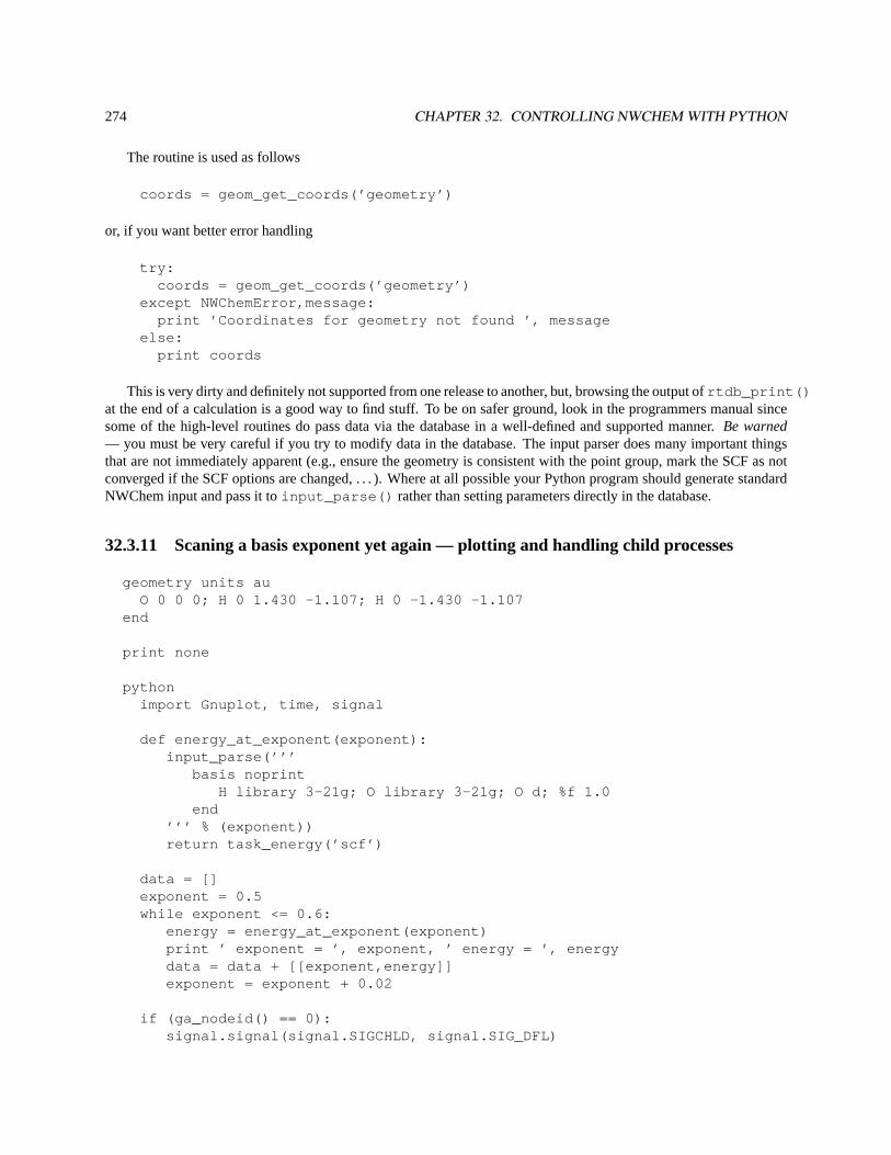
274 CHAPTER 32. CONTROLLING NWCHEM WITH PYTHON
The routine is used as follows
coords = geom_get_coords(’geometry’)
or, if you want better error handling
try:coords = geom_get_coords(’geometry’)
except NWChemError,message:print ’Coordinates for geometry not found ’, message
else:print coords
This is very dirty and definitely not supported from one release to another, but, browsing the output ofrtdb_print()at the end of a calculation is a good way to find stuff. To be on safer ground, look in the programmers manual sincesome of the high-level routines do pass data via the database in a well-defined and supported manner.Be warned— you must be very careful if you try to modify data in the database. The input parser does many important thingsthat are not immediately apparent (e.g., ensure the geometry is consistent with the point group, mark the SCF as notconverged if the SCF options are changed, . . . ). Where at all possible your Python program should generate standardNWChem input and pass it toinput_parse() rather than setting parameters directly in the database.
32.3.11 Scaning a basis exponent yet again — plotting and handling child processes
geometry units auO 0 0 0; H 0 1.430 -1.107; H 0 -1.430 -1.107
end
print none
pythonimport Gnuplot, time, signal
def energy_at_exponent(exponent):input_parse(’’’
basis noprintH library 3-21g; O library 3-21g; O d; %f 1.0
end’’’ % (exponent))return task_energy(’scf’)
data = []exponent = 0.5while exponent <= 0.6:
energy = energy_at_exponent(exponent)print ’ exponent = ’, exponent, ’ energy = ’, energydata = data + [[exponent,energy]]exponent = exponent + 0.02
if (ga_nodeid() == 0):signal.signal(signal.SIGCHLD, signal.SIG_DFL)
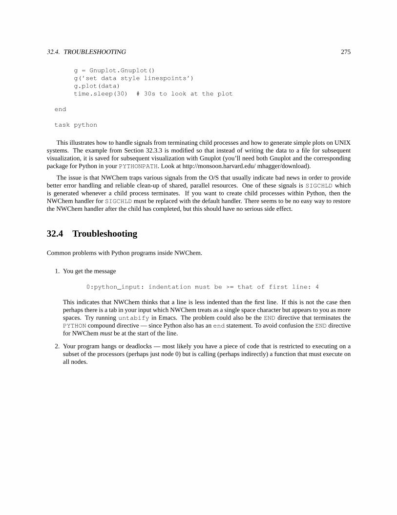
32.4. TROUBLESHOOTING 275
g = Gnuplot.Gnuplot()g(’set data style linespoints’)g.plot(data)time.sleep(30) # 30s to look at the plot
end
task python
This illustrates how to handle signals from terminating child processes and how to generate simple plots on UNIXsystems. The example from Section 32.3.3 is modified so that instead of writing the data to a file for subsequentvisualization, it is saved for subsequent visualization with Gnuplot (you’ll need both Gnuplot and the correspondingpackage for Python in yourPYTHONPATH. Look at http://monsoon.harvard.edu/ mhagger/download).
The issue is that NWChem traps various signals from the O/S that usually indicate bad news in order to providebetter error handling and reliable clean-up of shared, parallel resources. One of these signals isSIGCHLDwhichis generated whenever a child process terminates. If you want to create child processes within Python, then theNWChem handler forSIGCHLDmust be replaced with the default handler. There seems to be no easy way to restorethe NWChem handler after the child has completed, but this should have no serious side effect.
32.4 Troubleshooting
Common problems with Python programs inside NWChem.
1. You get the message
0:python_input: indentation must be >= that of first line: 4
This indicates that NWChem thinks that a line is less indented than the first line. If this is not the case thenperhaps there is a tab in your input which NWChem treats as a single space character but appears to you as morespaces. Try runninguntabify in Emacs. The problem could also be theENDdirective that terminates thePYTHONcompound directive — since Python also has anend statement. To avoid confusion theENDdirectivefor NWChemmustbe at the start of the line.
2. Your program hangs or deadlocks — most likely you have a piece of code that is restricted to executing on asubset of the processors (perhaps just node 0) but is calling (perhaps indirectly) a function that must execute onall nodes.

276 CHAPTER 32. CONTROLLING NWCHEM WITH PYTHON
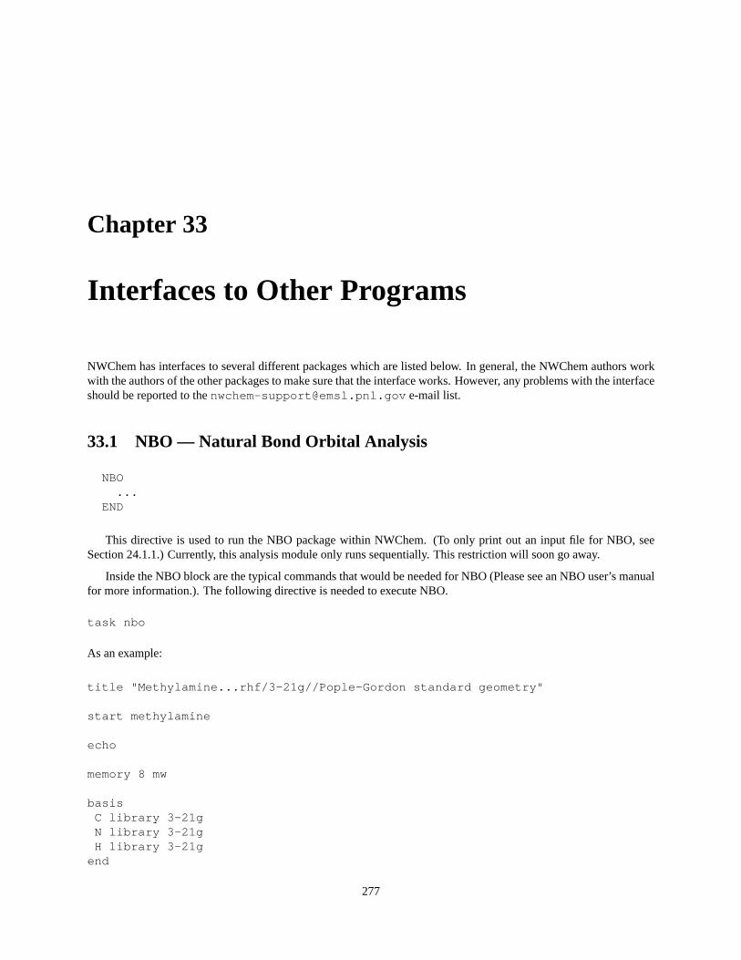
Chapter 33
Interfaces to Other Programs
NWChem has interfaces to several different packages which are listed below. In general, the NWChem authors workwith the authors of the other packages to make sure that the interface works. However, any problems with the interfaceshould be reported to [email protected] e-mail list.
33.1 NBO — Natural Bond Orbital Analysis
NBO...
END
This directive is used to run the NBO package within NWChem. (To only print out an input file for NBO, seeSection 24.1.1.) Currently, this analysis module only runs sequentially. This restriction will soon go away.
Inside the NBO block are the typical commands that would be needed for NBO (Please see an NBO user’s manualfor more information.). The following directive is needed to execute NBO.
task nbo
As an example:
title "Methylamine...rhf/3-21g//Pople-Gordon standard geometry"
start methylamine
echo
memory 8 mw
basisC library 3-21gN library 3-21gH library 3-21g
end
277
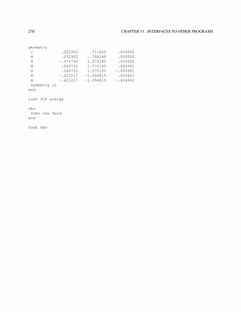
278 CHAPTER 33. INTERFACES TO OTHER PROGRAMS
geometryC .052902 .711852 .000000N .052902 -.758148 .000000H -.974760 1.075185 .000000H .566733 1.075185 .889981H .566733 1.075185 -.889981H -.423217 -1.094815 .824662H -.423217 -1.094815 -.824662symmetry c1
end
task SCF energy
nbo$nbo cmo $end
end
task nbo

Chapter 34
Acknowledgments
This work was supported by funds from the Environmental and Molecular Sciences Laboratory Construction Projectat Pacific Northwest National Laboratory. Development of some of the parallel programming tools and algorithmsemployed by NWChem was performed under the auspices of the High Performance Computing and CommunicationsProgram of the Mathematical, Information, and Computational Sciences Division, U.S. Department of Energy. PacificNorthwest National Laboratory is operated by Battelle Memorial Institute for the U.S. Department of Energy underContract DE-AC06-76RLO 1830.
279

280 CHAPTER 34. ACKNOWLEDGMENTS
Appendix A
Standard Basis Sets
Basis sets and effective core potentials were obtained (7/6/2000) from the Extensible Computational Chemistry En-vironment (ECCE) Basis Set Database, as developed and distributed by the Molecular Science Computing Facility,Environmental and Molecular Sciences Laboratory which is part of the Pacific Northwest National Laboratory, P.O.Box 999, Richland, Washington 99352, USA, and is funded by the U.S. Department of Energy. The Pacific North-west National Laboratory is a multi-program laboratory operated by Battelle Memorial Institute for the U.S. Depart-ment of Energy under contract DE-AC06-76RLO. Contact David Feller ([email protected] ) or Deborah Gracio([email protected] ) for further information.
The names in the NWChem library are consistent with those in the ECCE database and thus may include spaces.The standard NWChem input routines require that strings including spaces are enclosed in quotation marks ("..." )or that blanks are escaped with a backslash. As a convenience, basis set names may also have the blanks replaced withunderscores. Thus, the following all yield the same basis set for oxygen
oxygen library "DZP + Diffuse (Dunning)"oxygen library DZP\ +\ Diffuse\ (Dunning)oxygen library DZP_+_Diffuse_(Dunning)
Case may be ignored when specifying basis set names, but otherwise names should be specified exactly as providedbelow. A good method is just to cut/paste from the WWW pages since they were generated electronically from thelibrary source.
Errors found in the basis set library of NWChem version 3.3 have been corrected in the current library of NWChemversion 4.0. The changes are listed below:
1. Basis Set"Hay-Wadt VDZ (n+1) ECP"Element: AgCorrection of contraction coefficient in first s contraction.
2. Basis Set"LANL2DZ ECP"Element: AgCorrection of contraction coefficient in first s contraction.
3. Basis Set"CRENBS ECP"Element: All elements in the"CRENBS ECP"FamilyComplete revision of basis sets. The original sets were completely uncontracted and some of the first rowtransition metals were missing all of their d functions. The current sets relflect the minimal contraction of theoriginal papers.
281
282 APPENDIX A. STANDARD BASIS SETS
4. ECP"SBKJC VDZ ECP"Element: CeCorrection of switched integer powers for d-f component.
Relativistic contractions of standard basis sets for use in the Douglas-Kroll and Dyall-modified-Dirac method havealso been included in the library. These are identified by tags following the standard basis set name.
For the Douglas-Kroll method the tagdk should be specified:
oxygen library cc-pVDZ_DK
For the Dyall-modified-Dirac (DMD) method three tags should be specified. The first is a tag for the nuclearmodel, which can bept or fi for a point or a finite Gaussian model (see Section6). The second is a tag for therelativistic Hamiltonian:sf is for the spin-free modified Dirac Hamiltonian. The third tags the component type,fwfor the atomic FW transformed large component,lc for the large component andsc for the small component:
oxygen library cc-pvdz_pt_sf_fwoxygen library cc-pvdz_pt_sf_lc
Basis sets which are available with either the DmD or DK contractions are indicated in the list below.
Here is a list of known all-electron non-relativistic, DK and DmD basis sets, effective core potentials with theirrespective basis sets, and fitting basis sets along with the elements included for each. Additional information abouteach basis set in the NWChem library can be obtained from the online EMSL Gaussian Basis Set library.
Standard all-electron basis sets:
1. Basis Set"STO-2G" (number of atoms 20)H He Li Be B C N O F Ne Na Mg Al Si P S Cl Ar K Ca
2. Basis Set"STO-3G" (number of atoms 52)H He Li Be B C N O F Ne Na Mg Al Si P S Cl Ar K Ca Sc Ti V Cr Mn Fe Co Ni Cu Zn Ga Ge As Se Br Kr RbSr Y Zr Nb Mo Tc Ru Rh Pd Ag Cd In Sn Sb Te
3. Basis Set"STO-6G" (number of atoms 36)H He Li Be B C N O F Ne Na Mg Al Si P S Cl Ar K Ca Sc Ti V Cr Mn Fe Co Ni Cu Zn Ga Ge As Se Br Kr
4. Basis Set"STO-3G*" (number of atoms 18)H He Li Be B C N O F Ne Na Mg Al Si P S Cl Ar
5. Basis Set"3-21G" (number of atoms 55)H He Li Be B C N O F Ne Na Mg Al Si P S Cl Ar K Ca Sc Ti V Cr Mn Fe Co Ni Cu Zn Ga Ge As Se Br Kr RbSr Y Zr Nb Mo Tc Ru Rh Pd Ag Cd In Sn Sb Te I Xe Cs
6. Basis Set"3-21++G" (number of atoms 18)H He Li Be B C N O F Ne Na Mg Al Si P S Cl Ar
7. Basis Set"3-21G*" (number of atoms 17)H He Li Be B C N O F Ne Na Mg Al Si P S Cl
8. Basis Set"3-21++G*" (number of atoms 18)H He Li Be B C N O F Ne Na Mg Al Si P S Cl Ar
283
9. Basis Set"3-21GSP" (number of atoms 18)H He Li Be B C N O F Ne Na Mg Al Si P S Cl Ar
10. Basis Set"4-22GSP" (number of atoms 18)H He Li Be B C N O F Ne Na Mg Al Si P S Cl Ar
11. Basis Set"4-31G" (number of atoms 13)H He Li Be B C N O F Ne P S Cl
12. Basis Set"6-31G" (number of atoms 30)H He Li Be B C N O F Ne Na Mg Al Si P S Cl Ar K Ca Sc Ti V Cr Mn Fe Co Ni Cu Zn
13. Basis Set"6-31++G" (number of atoms 18)H He Li Be B C N O F Ne Na Mg Al Si P S Cl Ar
14. Basis Set"6-31G*" (number of atoms 30)H He Li Be B C N O F Ne Na Mg Al Si P S Cl Ar K Ca Sc Ti V Cr Mn Fe Co Ni Cu Zn
15. Basis Set"6-31G**" (number of atoms 30)H He Li Be B C N O F Ne Na Mg Al Si P S Cl Ar K Ca Sc Ti V Cr Mn Fe Co Ni Cu Zn
16. Basis Set"6-31+G*" (number of atoms 18)H He Li Be B C N O F Ne Na Mg Al Si P S Cl Ar
17. Basis Set"6-31++G*" (number of atoms 18)H He Li Be B C N O F Ne Na Mg Al Si P S Cl Ar
18. Basis Set"6-31++G**" (number of atoms 18)H He Li Be B C N O F Ne Na Mg Al Si P S Cl Ar
19. Basis Set"6-31G(3df,3pd)" (number of atoms 18)H He Li Be B C N O F Ne Na Mg Al Si P S Cl Ar
20. Basis Set"6-31G-Blaudeau" (number of atoms 2)K Ca
21. Basis Set"6-31G*-Blaudeau" (number of atoms 2)K Ca
22. Basis Set"6-311G" (number of atoms 24)H He Li Be B C N O F Ne Na Mg Al Si P S Cl Ar Ga Ge As Se Br Kr
23. Basis Set"6-311G*" (number of atoms 24)H He Li Be B C N O F Ne Na Mg Al Si P S Cl Ar Ga Ge As Se Br Kr
24. Basis Set"6-311G**" (number of atoms 24)H He Li Be B C N O F Ne Na Mg Al Si P S Cl Ar Ga Ge As Se Br Kr
25. Basis Set"6-311++G**" (number of atoms 10)H He Li Be B C N O F Ne
26. Basis Set"6-311++G(2d,2p)" (number of atoms 10)H He Li Be B C N O F Ne
27. Basis Set"6-311G(2df,2pd)" (number of atoms 10)H He Li Be B C N O F Ne

284 APPENDIX A. STANDARD BASIS SETS
28. Basis Set"6-311+G*" (number of atoms 10)H He Li Be B C N O F Ne
29. Basis Set"6-311++G(3df,3pd)" (number of atoms 18)H He Li Be B C N O F Ne Na Mg Al Si P S Cl Ar
30. Basis Set"MINI (Huzinaga)" (number of atoms 18)H He Li Be B C N O F Ne Na Mg Al Si P S Cl Ar
31. Basis Set"MINI (Scaled)" (number of atoms 20)H He Li Be B C N O F Ne Na Mg Al Si P S Cl Ar K Ca
32. Basis Set"MIDI (Huzinaga)" (number of atoms 18)H He Li Be B C N O F Ne Na Al Si P S Cl Ar K
33. Basis Set"MIDI!" (number of atoms 11)H C N O F Si P S Cl Br I
34. Basis Set"SV (Dunning-Hay)" (number of atoms 9)H Li Be B C N O F Ne
35. Basis Set"SVP (Dunning-Hay)" (number of atoms 9)H Li Be B C N O F Ne
36. Basis Set"SVP + Diffuse (Dunning-Hay)" (number of atoms 9)H Li Be B C N O F Ne
37. Basis Set"TZ (Dunning)" (number of atoms 8)H Li B C N O F Ne
38. Basis Set"Chipman DZP + Diffuse" (number of atoms 6)H B C N O F
39. Basis Set"DZ (Dunning)" (number of atoms 12)H B C N O F Ne Al Si P S Cl
40. Basis Set"DZP (Dunning)" (number of atoms 12)H B C N O F Ne Al Si P S Cl
41. Basis Set"DZP + Diffuse (Dunning)" (number of atoms 7)H B C N O F Ne
42. Basis Set"cc-pVDZ" (number of atoms 20)H He B C N O F Ne Al Si P S Cl Ar Ga Ge As Se Br Kr
43. Basis Set"cc-pVTZ" (number of atoms 20)H He B C N O F Ne Al Si P S Cl Ar Ga Ge As Se Br Kr
44. Basis Set"cc-pVQZ" (number of atoms 20)H He B C N O F Ne Al Si P S Cl Ar Ga Ge As Se Br Kr
45. Basis Set"cc-pV5Z" (number of atoms 21)H He Li B C N O F Ne Al Si P S Cl Ar Ga Ge As Se Br Kr
46. Basis Set"cc-pV6Z" (number of atoms 14)H He B C N O F Ne Al Si P S Cl Ar

285
47. Basis Set"cc-pCVDZ" (number of atoms 6)B C N O F Ne
48. Basis Set"cc-pCVTZ" (number of atoms 6)B C N O F Ne
49. Basis Set"cc-pCVQZ" (number of atoms 6)B C N O F Ne
50. Basis Set"cc-pCV5Z" (number of atoms 6)B C N O F Ne
51. Basis Set"aug-cc-pVDZ" (number of atoms 20)H He B C N O F Ne Al Si P S Cl Ar Ga Ge As Se Br Kr
52. Basis Set"aug-cc-pVTZ" (number of atoms 20)H He B C N O F Ne Al Si P S Cl Ar Ga Ge As Se Br Kr
53. Basis Set"aug-cc-pVQZ" (number of atoms 20)H He B C N O F Ne Al Si P S Cl Ar Ga Ge As Se Br Kr
54. Basis Set"aug-cc-pV5Z" (number of atoms 20)H He B C N O F Ne Al Si P S Cl Ar Ga Ge As Se Br Kr
55. Basis Set"aug-cc-pV6Z" (number of atoms 14)H He B C N O F Ne Al Si P S Cl Ar
56. Basis Set"aug-cc-pCVDZ" (number of atoms 5)B C N O F
57. Basis Set"aug-cc-pCVTZ" (number of atoms 6)B C N O F Ne
58. Basis Set"aug-cc-pCVQZ" (number of atoms 6)B C N O F Ne
59. Basis Set"aug-cc-pCV5Z" (number of atoms 5)B C N O F
60. Basis Set"d-aug-cc-pVDZ" (number of atoms 8)H He B C N O F Ne
61. Basis Set"d-aug-cc-pVTZ" (number of atoms 8)H He B C N O F Ne
62. Basis Set"d-aug-cc-pVQZ" (number of atoms 8)H He B C N O F Ne
63. Basis Set"d-aug-cc-pV5Z" (number of atoms 8)H He B C N O F Ne
64. Basis Set"d-aug-cc-pV6Z" (number of atoms 5)H B C N O
65. Basis Set"GAMESS VTZ"(number of atoms 8)H Be B C N O F Ne
286 APPENDIX A. STANDARD BASIS SETS
66. Basis Set"GAMESS PVTZ"(number of atoms 8)H Be B C N O F Ne
67. Basis Set"Partridge Uncontr. 1" (number of atoms 34)Li Be B C N O F Ne Na Mg Al Si P S Cl Ar K Ca Sc Ti V Cr Mn Fe Co Ni Cu Zn Ga Ge As Se Br Kr
68. Basis Set"Partridge Uncontr. 2" (number of atoms 34)Li Be B C N O F Ne Na Mg Al Si P S Cl Ar K Ca Sc Ti V Cr Mn Fe Co Ni Cu Zn Ga Ge As Se Br Kr
69. Basis Set"Partridge Uncontr. 3" (number of atoms 28)Li Be B C N O F Ne Na Mg Al Si P S Cl Ar K Ca Sc Ti V Cr Mn Fe Co Ni Cu Zn
70. Basis Set"Ahlrichs VDZ" (number of atoms 36)H He Li Be B C N O F Ne Na Mg Al Si P S Cl Ar K Ca Sc Ti V Cr Mn Fe Co Ni Cu Zn Ga Ge As Se Br Kr
71. Basis Set"Ahlrichs pVDZ" (number of atoms 36)H He Li Be B C N O F Ne Na Mg Al Si P S Cl Ar K Ca Sc Ti V Cr Mn Fe Co Ni Cu Zn Ga Ge As Se Br Kr
72. Basis Set"Ahlrichs VTZ" (number of atoms 36)H He Li Be B C N O F Ne Na Mg Al Si P S Cl Ar K Ca Sc Ti V Cr Mn Fe Co Ni Cu Zn Ga Ge As Se Br Kr
73. Basis Set"Binning/Curtiss SV" (number of atoms 6)Ga Ge As Se Br Kr
74. Basis Set"Binning/Curtiss VTZ" (number of atoms 6)Ga Ge As Se Br Kr
75. Basis Set"Binning/Curtiss SVP" (number of atoms 6)Ga Ge As Se Br Kr
76. Basis Set"Binning/Curtiss VTZP" (number of atoms 6)Ga Ge As Se Br Kr
77. Basis Set"McLean/Chandler VTZ" (number of atoms 8)Na Mg Al Si P S Cl Ar
78. Basis Set"SV + Rydberg (Dunning-Hay)" (number of atoms 9)H Li Be B C N O F Ne
79. Basis Set"SVP + Rydberg (Dunning-Hay)" (number of atoms 9)H Li Be B C N O F Ne
80. Basis Set"SVP + Diffuse + Rydberg" (number of atoms 9)H Li Be B C N O F Ne
81. Basis Set"DZ + Rydberg (Dunning)" (number of atoms 12)H B C N O F Ne Al Si P S Cl
82. Basis Set"DZP + Rydberg (Dunning)" (number of atoms 12)H B C N O F Ne Al Si P S Cl
83. Basis Set"DZ + Double Rydberg (Dunning-Hay)" (number of atoms 12)H B C N O F Ne Al Si P S Cl
84. Basis Set"SV + Double Rydberg (Dunning-Hay)" (number of atoms 9)H Li Be B C N O F Ne

287
85. Basis Set"Wachters+f" (number of atoms 9)Sc Ti V Cr Mn Fe Co Ni Cu
86. Basis Set"Bauschlicher ANO" (number of atoms 9)Sc Ti V Cr Mn Fe Co Ni Cu
87. Basis Set"NASA Ames ANO"(number of atoms 12)H B C N O F Ne Al P Ti Fe Ni
88. Basis Set"Sadlej pVTZ" (number of atoms 18)H Li Be C N O F Na Mg Si P S Cl K Ca Br Rb Sr
89. Basis Set"WTBS" (number of atoms 84)He Li Be B C N O F Ne Na Mg Al Si P S Cl Ar K Ca Sc Ti V Cr Mn Fe Co Ni Cu Zn Ga Ge As Se Br Kr RbSr Y Zr Nb Mo Tc Ru Rh Pd Ag Cd In Sn Sb Te I Xe Cs Ba La Ce Pr Pm Sm Eu Gd Tb Dy Ho Er Tm Yb LuHf Ta W Re Os Ir Pt Au Hg Tl Pb Bi Po At Rn
Resolution of Identity (RI) fitting basis sets:
1. Basis Set"cc-pVDZ-fit2-1" (number of atoms 10)H He Li Be B C N O F Ne
2. Basis Set"cc-pVTZ-fit2-1" (number of atoms 10)H He Li Be B C N O F Ne
Density functional specific basis sets:
1. Basis Set"DZVP (DFT Orbital)" (number of atoms 54)H He Li Be B C N O F Ne Na Mg Al Si P S Cl Ar K Ca Sc Ti V Cr Mn Fe Co Ni Cu Zn Ga Ge As Se Br Kr RbSr Y Zr Nb Mo Tc Ru Rh Pd Ag Cd In Sn Sb Te I Xe
2. Basis Set"DZVP2 (DFT Orbital)" (number of atoms 25)H He Li Be B C N O F Al Si P S Cl Ar Sc Ti V Cr Mn Fe Co Ni Cu Zn
3. Basis Set"TZVP (DFT Orbital)" (number of atoms 11)H C N O F Al Si P S Cl Ar
Density functional Coulomb and Exchange fitting basis sets:
1. Basis Set"DGauss A1 DFT Coulomb Fitting" (number of atoms 54)H He Li Be B C N O F Ne Na Mg Al Si P S Cl Ar K Ca Sc Ti V Cr Mn Fe Co Ni Cu Zn Ga Ge As Se Br Kr RbSr Y Zr Nb Mo Tc Ru Rh Pd Ag Cd In Sn Sb Te I Xe
2. Basis Set"DGauss A1 DFT Exchange Fitting" (number of atoms 54)H He Li Be B C N O F Ne Na Mg Al Si P S Cl Ar K Ca Sc Ti V Cr Mn Fe Co Ni Cu Zn Ga Ge As Se Br Kr RbSr Y Zr Nb Mo Tc Ru Rh Pd Ag Cd In Sn Sb Te I Xe
3. Basis Set"DGauss A2 DFT Coulomb Fitting" (number of atoms 25)H He Li Be B C N O F Al Si P S Cl Ar Sc Ti V Cr Mn Fe Co Ni Cu Zn
4. Basis Set"DGauss A2 DFT Exchange Fitting" (number of atoms 25)H He Li Be B C N O F Al Si P S Cl Ar Sc Ti V Cr Mn Fe Co Ni Cu Zn
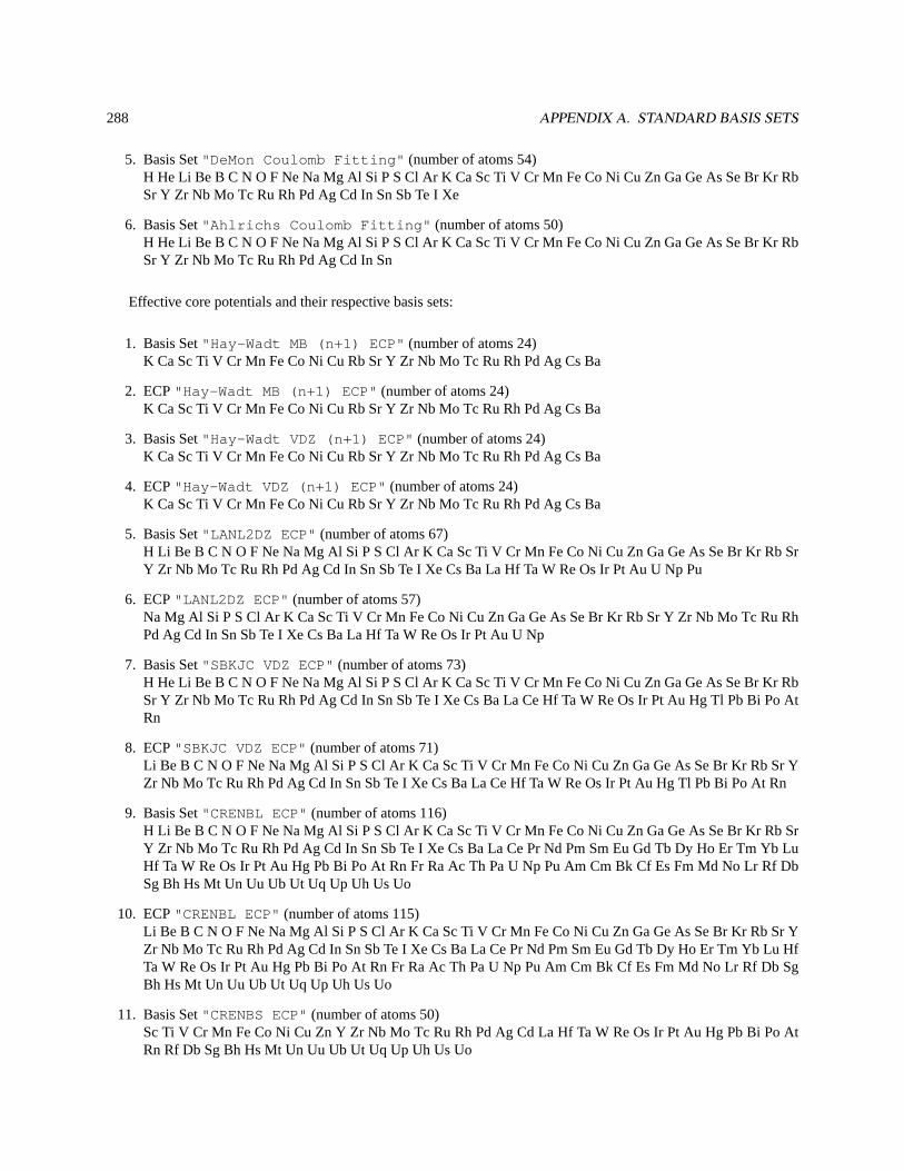
288 APPENDIX A. STANDARD BASIS SETS
5. Basis Set"DeMon Coulomb Fitting" (number of atoms 54)H He Li Be B C N O F Ne Na Mg Al Si P S Cl Ar K Ca Sc Ti V Cr Mn Fe Co Ni Cu Zn Ga Ge As Se Br Kr RbSr Y Zr Nb Mo Tc Ru Rh Pd Ag Cd In Sn Sb Te I Xe
6. Basis Set"Ahlrichs Coulomb Fitting" (number of atoms 50)H He Li Be B C N O F Ne Na Mg Al Si P S Cl Ar K Ca Sc Ti V Cr Mn Fe Co Ni Cu Zn Ga Ge As Se Br Kr RbSr Y Zr Nb Mo Tc Ru Rh Pd Ag Cd In Sn
Effective core potentials and their respective basis sets:
1. Basis Set"Hay-Wadt MB (n+1) ECP" (number of atoms 24)K Ca Sc Ti V Cr Mn Fe Co Ni Cu Rb Sr Y Zr Nb Mo Tc Ru Rh Pd Ag Cs Ba
2. ECP"Hay-Wadt MB (n+1) ECP" (number of atoms 24)K Ca Sc Ti V Cr Mn Fe Co Ni Cu Rb Sr Y Zr Nb Mo Tc Ru Rh Pd Ag Cs Ba
3. Basis Set"Hay-Wadt VDZ (n+1) ECP" (number of atoms 24)K Ca Sc Ti V Cr Mn Fe Co Ni Cu Rb Sr Y Zr Nb Mo Tc Ru Rh Pd Ag Cs Ba
4. ECP"Hay-Wadt VDZ (n+1) ECP" (number of atoms 24)K Ca Sc Ti V Cr Mn Fe Co Ni Cu Rb Sr Y Zr Nb Mo Tc Ru Rh Pd Ag Cs Ba
5. Basis Set"LANL2DZ ECP" (number of atoms 67)H Li Be B C N O F Ne Na Mg Al Si P S Cl Ar K Ca Sc Ti V Cr Mn Fe Co Ni Cu Zn Ga Ge As Se Br Kr Rb SrY Zr Nb Mo Tc Ru Rh Pd Ag Cd In Sn Sb Te I Xe Cs Ba La Hf Ta W Re Os Ir Pt Au U Np Pu
6. ECP"LANL2DZ ECP" (number of atoms 57)Na Mg Al Si P S Cl Ar K Ca Sc Ti V Cr Mn Fe Co Ni Cu Zn Ga Ge As Se Br Kr Rb Sr Y Zr Nb Mo Tc Ru RhPd Ag Cd In Sn Sb Te I Xe Cs Ba La Hf Ta W Re Os Ir Pt Au U Np
7. Basis Set"SBKJC VDZ ECP"(number of atoms 73)H He Li Be B C N O F Ne Na Mg Al Si P S Cl Ar K Ca Sc Ti V Cr Mn Fe Co Ni Cu Zn Ga Ge As Se Br Kr RbSr Y Zr Nb Mo Tc Ru Rh Pd Ag Cd In Sn Sb Te I Xe Cs Ba La Ce Hf Ta W Re Os Ir Pt Au Hg Tl Pb Bi Po AtRn
8. ECP"SBKJC VDZ ECP"(number of atoms 71)Li Be B C N O F Ne Na Mg Al Si P S Cl Ar K Ca Sc Ti V Cr Mn Fe Co Ni Cu Zn Ga Ge As Se Br Kr Rb Sr YZr Nb Mo Tc Ru Rh Pd Ag Cd In Sn Sb Te I Xe Cs Ba La Ce Hf Ta W Re Os Ir Pt Au Hg Tl Pb Bi Po At Rn
9. Basis Set"CRENBL ECP"(number of atoms 116)H Li Be B C N O F Ne Na Mg Al Si P S Cl Ar K Ca Sc Ti V Cr Mn Fe Co Ni Cu Zn Ga Ge As Se Br Kr Rb SrY Zr Nb Mo Tc Ru Rh Pd Ag Cd In Sn Sb Te I Xe Cs Ba La Ce Pr Nd Pm Sm Eu Gd Tb Dy Ho Er Tm Yb LuHf Ta W Re Os Ir Pt Au Hg Pb Bi Po At Rn Fr Ra Ac Th Pa U Np Pu Am Cm Bk Cf Es Fm Md No Lr Rf DbSg Bh Hs Mt Un Uu Ub Ut Uq Up Uh Us Uo
10. ECP"CRENBL ECP"(number of atoms 115)Li Be B C N O F Ne Na Mg Al Si P S Cl Ar K Ca Sc Ti V Cr Mn Fe Co Ni Cu Zn Ga Ge As Se Br Kr Rb Sr YZr Nb Mo Tc Ru Rh Pd Ag Cd In Sn Sb Te I Xe Cs Ba La Ce Pr Nd Pm Sm Eu Gd Tb Dy Ho Er Tm Yb Lu HfTa W Re Os Ir Pt Au Hg Pb Bi Po At Rn Fr Ra Ac Th Pa U Np Pu Am Cm Bk Cf Es Fm Md No Lr Rf Db SgBh Hs Mt Un Uu Ub Ut Uq Up Uh Us Uo
11. Basis Set"CRENBS ECP"(number of atoms 50)Sc Ti V Cr Mn Fe Co Ni Cu Zn Y Zr Nb Mo Tc Ru Rh Pd Ag Cd La Hf Ta W Re Os Ir Pt Au Hg Pb Bi Po AtRn Rf Db Sg Bh Hs Mt Un Uu Ub Ut Uq Up Uh Us Uo
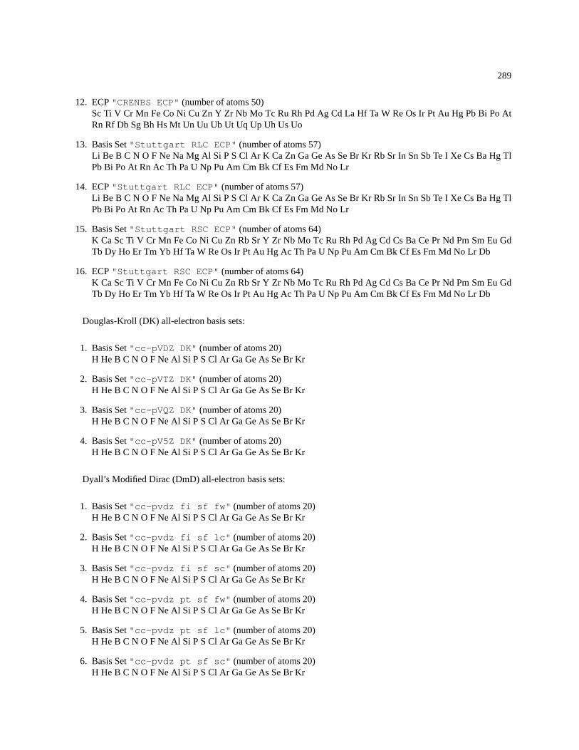
289
12. ECP"CRENBS ECP"(number of atoms 50)Sc Ti V Cr Mn Fe Co Ni Cu Zn Y Zr Nb Mo Tc Ru Rh Pd Ag Cd La Hf Ta W Re Os Ir Pt Au Hg Pb Bi Po AtRn Rf Db Sg Bh Hs Mt Un Uu Ub Ut Uq Up Uh Us Uo
13. Basis Set"Stuttgart RLC ECP" (number of atoms 57)Li Be B C N O F Ne Na Mg Al Si P S Cl Ar K Ca Zn Ga Ge As Se Br Kr Rb Sr In Sn Sb Te I Xe Cs Ba Hg TlPb Bi Po At Rn Ac Th Pa U Np Pu Am Cm Bk Cf Es Fm Md No Lr
14. ECP"Stuttgart RLC ECP" (number of atoms 57)Li Be B C N O F Ne Na Mg Al Si P S Cl Ar K Ca Zn Ga Ge As Se Br Kr Rb Sr In Sn Sb Te I Xe Cs Ba Hg TlPb Bi Po At Rn Ac Th Pa U Np Pu Am Cm Bk Cf Es Fm Md No Lr
15. Basis Set"Stuttgart RSC ECP" (number of atoms 64)K Ca Sc Ti V Cr Mn Fe Co Ni Cu Zn Rb Sr Y Zr Nb Mo Tc Ru Rh Pd Ag Cd Cs Ba Ce Pr Nd Pm Sm Eu GdTb Dy Ho Er Tm Yb Hf Ta W Re Os Ir Pt Au Hg Ac Th Pa U Np Pu Am Cm Bk Cf Es Fm Md No Lr Db
16. ECP"Stuttgart RSC ECP" (number of atoms 64)K Ca Sc Ti V Cr Mn Fe Co Ni Cu Zn Rb Sr Y Zr Nb Mo Tc Ru Rh Pd Ag Cd Cs Ba Ce Pr Nd Pm Sm Eu GdTb Dy Ho Er Tm Yb Hf Ta W Re Os Ir Pt Au Hg Ac Th Pa U Np Pu Am Cm Bk Cf Es Fm Md No Lr Db
Douglas-Kroll (DK) all-electron basis sets:
1. Basis Set"cc-pVDZ DK" (number of atoms 20)H He B C N O F Ne Al Si P S Cl Ar Ga Ge As Se Br Kr
2. Basis Set"cc-pVTZ DK" (number of atoms 20)H He B C N O F Ne Al Si P S Cl Ar Ga Ge As Se Br Kr
3. Basis Set"cc-pVQZ DK" (number of atoms 20)H He B C N O F Ne Al Si P S Cl Ar Ga Ge As Se Br Kr
4. Basis Set"cc-pV5Z DK" (number of atoms 20)H He B C N O F Ne Al Si P S Cl Ar Ga Ge As Se Br Kr
Dyall’s Modified Dirac (DmD) all-electron basis sets:
1. Basis Set"cc-pvdz fi sf fw" (number of atoms 20)H He B C N O F Ne Al Si P S Cl Ar Ga Ge As Se Br Kr
2. Basis Set"cc-pvdz fi sf lc" (number of atoms 20)H He B C N O F Ne Al Si P S Cl Ar Ga Ge As Se Br Kr
3. Basis Set"cc-pvdz fi sf sc" (number of atoms 20)H He B C N O F Ne Al Si P S Cl Ar Ga Ge As Se Br Kr
4. Basis Set"cc-pvdz pt sf fw" (number of atoms 20)H He B C N O F Ne Al Si P S Cl Ar Ga Ge As Se Br Kr
5. Basis Set"cc-pvdz pt sf lc" (number of atoms 20)H He B C N O F Ne Al Si P S Cl Ar Ga Ge As Se Br Kr
6. Basis Set"cc-pvdz pt sf sc" (number of atoms 20)H He B C N O F Ne Al Si P S Cl Ar Ga Ge As Se Br Kr
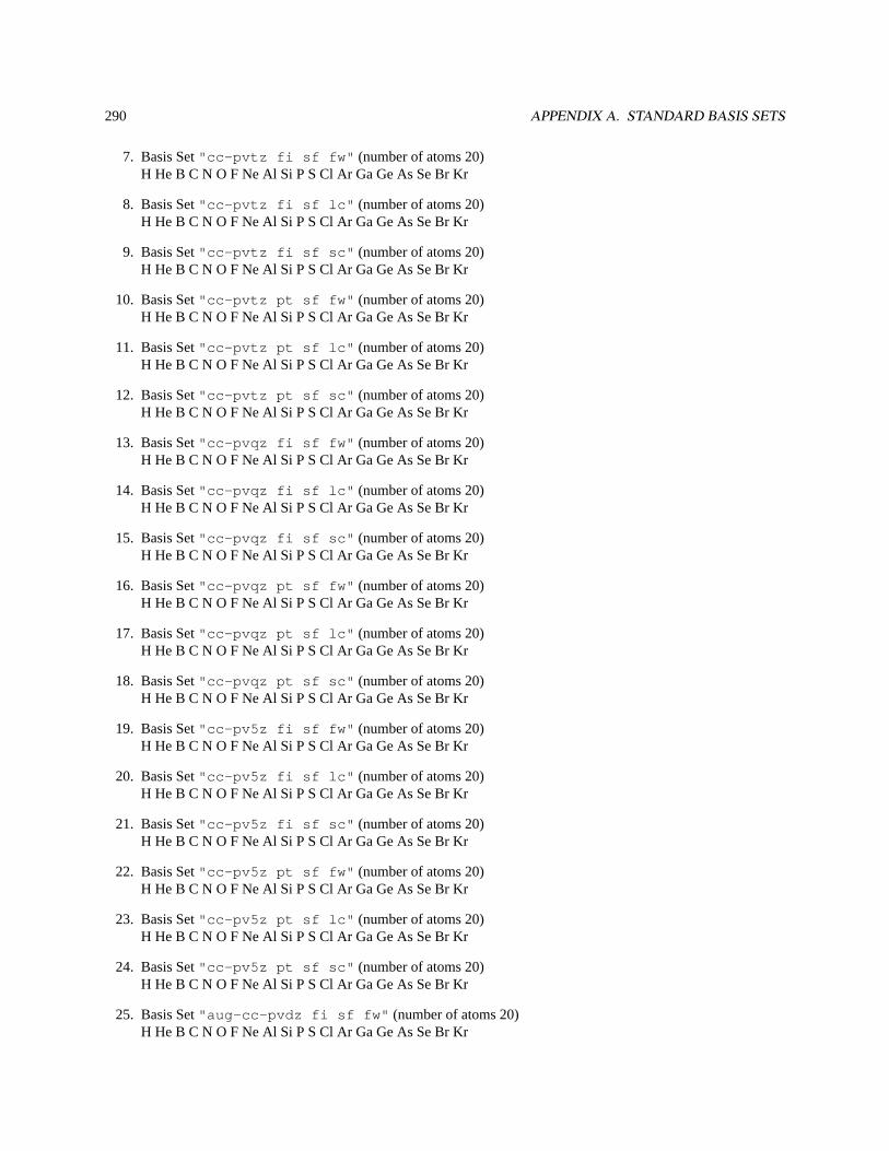
290 APPENDIX A. STANDARD BASIS SETS
7. Basis Set"cc-pvtz fi sf fw" (number of atoms 20)H He B C N O F Ne Al Si P S Cl Ar Ga Ge As Se Br Kr
8. Basis Set"cc-pvtz fi sf lc" (number of atoms 20)H He B C N O F Ne Al Si P S Cl Ar Ga Ge As Se Br Kr
9. Basis Set"cc-pvtz fi sf sc" (number of atoms 20)H He B C N O F Ne Al Si P S Cl Ar Ga Ge As Se Br Kr
10. Basis Set"cc-pvtz pt sf fw" (number of atoms 20)H He B C N O F Ne Al Si P S Cl Ar Ga Ge As Se Br Kr
11. Basis Set"cc-pvtz pt sf lc" (number of atoms 20)H He B C N O F Ne Al Si P S Cl Ar Ga Ge As Se Br Kr
12. Basis Set"cc-pvtz pt sf sc" (number of atoms 20)H He B C N O F Ne Al Si P S Cl Ar Ga Ge As Se Br Kr
13. Basis Set"cc-pvqz fi sf fw" (number of atoms 20)H He B C N O F Ne Al Si P S Cl Ar Ga Ge As Se Br Kr
14. Basis Set"cc-pvqz fi sf lc" (number of atoms 20)H He B C N O F Ne Al Si P S Cl Ar Ga Ge As Se Br Kr
15. Basis Set"cc-pvqz fi sf sc" (number of atoms 20)H He B C N O F Ne Al Si P S Cl Ar Ga Ge As Se Br Kr
16. Basis Set"cc-pvqz pt sf fw" (number of atoms 20)H He B C N O F Ne Al Si P S Cl Ar Ga Ge As Se Br Kr
17. Basis Set"cc-pvqz pt sf lc" (number of atoms 20)H He B C N O F Ne Al Si P S Cl Ar Ga Ge As Se Br Kr
18. Basis Set"cc-pvqz pt sf sc" (number of atoms 20)H He B C N O F Ne Al Si P S Cl Ar Ga Ge As Se Br Kr
19. Basis Set"cc-pv5z fi sf fw" (number of atoms 20)H He B C N O F Ne Al Si P S Cl Ar Ga Ge As Se Br Kr
20. Basis Set"cc-pv5z fi sf lc" (number of atoms 20)H He B C N O F Ne Al Si P S Cl Ar Ga Ge As Se Br Kr
21. Basis Set"cc-pv5z fi sf sc" (number of atoms 20)H He B C N O F Ne Al Si P S Cl Ar Ga Ge As Se Br Kr
22. Basis Set"cc-pv5z pt sf fw" (number of atoms 20)H He B C N O F Ne Al Si P S Cl Ar Ga Ge As Se Br Kr
23. Basis Set"cc-pv5z pt sf lc" (number of atoms 20)H He B C N O F Ne Al Si P S Cl Ar Ga Ge As Se Br Kr
24. Basis Set"cc-pv5z pt sf sc" (number of atoms 20)H He B C N O F Ne Al Si P S Cl Ar Ga Ge As Se Br Kr
25. Basis Set"aug-cc-pvdz fi sf fw" (number of atoms 20)H He B C N O F Ne Al Si P S Cl Ar Ga Ge As Se Br Kr
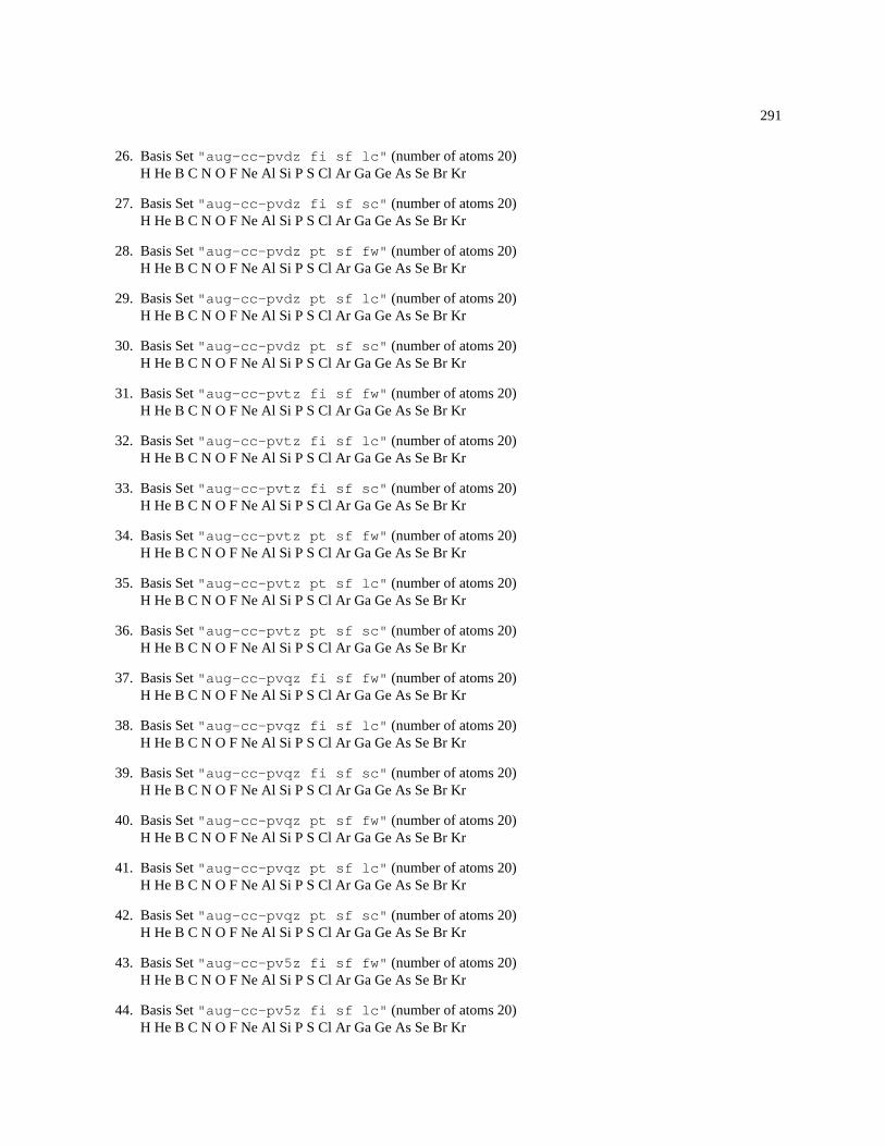
291
26. Basis Set"aug-cc-pvdz fi sf lc" (number of atoms 20)H He B C N O F Ne Al Si P S Cl Ar Ga Ge As Se Br Kr
27. Basis Set"aug-cc-pvdz fi sf sc" (number of atoms 20)H He B C N O F Ne Al Si P S Cl Ar Ga Ge As Se Br Kr
28. Basis Set"aug-cc-pvdz pt sf fw" (number of atoms 20)H He B C N O F Ne Al Si P S Cl Ar Ga Ge As Se Br Kr
29. Basis Set"aug-cc-pvdz pt sf lc" (number of atoms 20)H He B C N O F Ne Al Si P S Cl Ar Ga Ge As Se Br Kr
30. Basis Set"aug-cc-pvdz pt sf sc" (number of atoms 20)H He B C N O F Ne Al Si P S Cl Ar Ga Ge As Se Br Kr
31. Basis Set"aug-cc-pvtz fi sf fw" (number of atoms 20)H He B C N O F Ne Al Si P S Cl Ar Ga Ge As Se Br Kr
32. Basis Set"aug-cc-pvtz fi sf lc" (number of atoms 20)H He B C N O F Ne Al Si P S Cl Ar Ga Ge As Se Br Kr
33. Basis Set"aug-cc-pvtz fi sf sc" (number of atoms 20)H He B C N O F Ne Al Si P S Cl Ar Ga Ge As Se Br Kr
34. Basis Set"aug-cc-pvtz pt sf fw" (number of atoms 20)H He B C N O F Ne Al Si P S Cl Ar Ga Ge As Se Br Kr
35. Basis Set"aug-cc-pvtz pt sf lc" (number of atoms 20)H He B C N O F Ne Al Si P S Cl Ar Ga Ge As Se Br Kr
36. Basis Set"aug-cc-pvtz pt sf sc" (number of atoms 20)H He B C N O F Ne Al Si P S Cl Ar Ga Ge As Se Br Kr
37. Basis Set"aug-cc-pvqz fi sf fw" (number of atoms 20)H He B C N O F Ne Al Si P S Cl Ar Ga Ge As Se Br Kr
38. Basis Set"aug-cc-pvqz fi sf lc" (number of atoms 20)H He B C N O F Ne Al Si P S Cl Ar Ga Ge As Se Br Kr
39. Basis Set"aug-cc-pvqz fi sf sc" (number of atoms 20)H He B C N O F Ne Al Si P S Cl Ar Ga Ge As Se Br Kr
40. Basis Set"aug-cc-pvqz pt sf fw" (number of atoms 20)H He B C N O F Ne Al Si P S Cl Ar Ga Ge As Se Br Kr
41. Basis Set"aug-cc-pvqz pt sf lc" (number of atoms 20)H He B C N O F Ne Al Si P S Cl Ar Ga Ge As Se Br Kr
42. Basis Set"aug-cc-pvqz pt sf sc" (number of atoms 20)H He B C N O F Ne Al Si P S Cl Ar Ga Ge As Se Br Kr
43. Basis Set"aug-cc-pv5z fi sf fw" (number of atoms 20)H He B C N O F Ne Al Si P S Cl Ar Ga Ge As Se Br Kr
44. Basis Set"aug-cc-pv5z fi sf lc" (number of atoms 20)H He B C N O F Ne Al Si P S Cl Ar Ga Ge As Se Br Kr
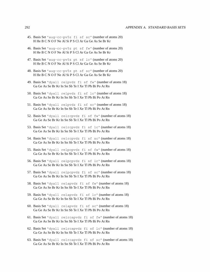
292 APPENDIX A. STANDARD BASIS SETS
45. Basis Set"aug-cc-pv5z fi sf sc" (number of atoms 20)H He B C N O F Ne Al Si P S Cl Ar Ga Ge As Se Br Kr
46. Basis Set"aug-cc-pv5z pt sf fw" (number of atoms 20)H He B C N O F Ne Al Si P S Cl Ar Ga Ge As Se Br Kr
47. Basis Set"aug-cc-pv5z pt sf lc" (number of atoms 20)H He B C N O F Ne Al Si P S Cl Ar Ga Ge As Se Br Kr
48. Basis Set"aug-cc-pv5z pt sf sc" (number of atoms 20)H He B C N O F Ne Al Si P S Cl Ar Ga Ge As Se Br Kr
49. Basis Set"dyall relpvdz fi sf fw" (number of atoms 18)Ga Ge As Se Br Kr In Sn Sb Te I Xe Tl Pb Bi Po At Rn
50. Basis Set"dyall relpvdz fi sf lc" (number of atoms 18)Ga Ge As Se Br Kr In Sn Sb Te I Xe Tl Pb Bi Po At Rn
51. Basis Set"dyall relpvdz fi sf sc" (number of atoms 18)Ga Ge As Se Br Kr In Sn Sb Te I Xe Tl Pb Bi Po At Rn
52. Basis Set"dyall relrcpvdz fi sf fw" (number of atoms 18)Ga Ge As Se Br Kr In Sn Sb Te I Xe Tl Pb Bi Po At Rn
53. Basis Set"dyall relrcpvdz fi sf lc" (number of atoms 18)Ga Ge As Se Br Kr In Sn Sb Te I Xe Tl Pb Bi Po At Rn
54. Basis Set"dyall relrcpvdz fi sf sc" (number of atoms 18)Ga Ge As Se Br Kr In Sn Sb Te I Xe Tl Pb Bi Po At Rn
55. Basis Set"dyall relpcpvdz fi sf fw" (number of atoms 18)Ga Ge As Se Br Kr In Sn Sb Te I Xe Tl Pb Bi Po At Rn
56. Basis Set"dyall relpcpvdz fi sf lc" (number of atoms 18)Ga Ge As Se Br Kr In Sn Sb Te I Xe Tl Pb Bi Po At Rn
57. Basis Set"dyall relpcpvdz fi sf sc" (number of atoms 18)Ga Ge As Se Br Kr In Sn Sb Te I Xe Tl Pb Bi Po At Rn
58. Basis Set"dyall relapvdz fi sf fw" (number of atoms 18)Ga Ge As Se Br Kr In Sn Sb Te I Xe Tl Pb Bi Po At Rn
59. Basis Set"dyall relapvdz fi sf lc" (number of atoms 18)Ga Ge As Se Br Kr In Sn Sb Te I Xe Tl Pb Bi Po At Rn
60. Basis Set"dyall relapvdz fi sf sc" (number of atoms 18)Ga Ge As Se Br Kr In Sn Sb Te I Xe Tl Pb Bi Po At Rn
61. Basis Set"dyall relrcapvdz fi sf fw" (number of atoms 18)Ga Ge As Se Br Kr In Sn Sb Te I Xe Tl Pb Bi Po At Rn
62. Basis Set"dyall relrcapvdz fi sf lc" (number of atoms 18)Ga Ge As Se Br Kr In Sn Sb Te I Xe Tl Pb Bi Po At Rn
63. Basis Set"dyall relrcapvdz fi sf sc" (number of atoms 18)Ga Ge As Se Br Kr In Sn Sb Te I Xe Tl Pb Bi Po At Rn
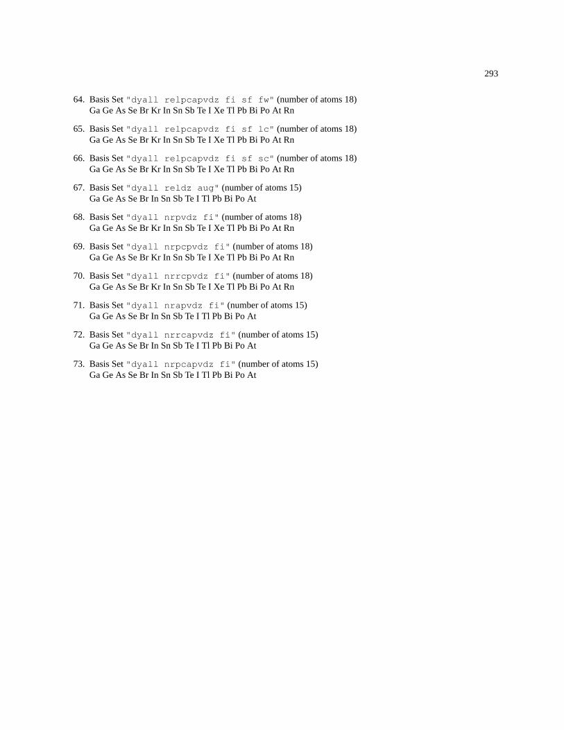
293
64. Basis Set"dyall relpcapvdz fi sf fw" (number of atoms 18)Ga Ge As Se Br Kr In Sn Sb Te I Xe Tl Pb Bi Po At Rn
65. Basis Set"dyall relpcapvdz fi sf lc" (number of atoms 18)Ga Ge As Se Br Kr In Sn Sb Te I Xe Tl Pb Bi Po At Rn
66. Basis Set"dyall relpcapvdz fi sf sc" (number of atoms 18)Ga Ge As Se Br Kr In Sn Sb Te I Xe Tl Pb Bi Po At Rn
67. Basis Set"dyall reldz aug" (number of atoms 15)Ga Ge As Se Br In Sn Sb Te I Tl Pb Bi Po At
68. Basis Set"dyall nrpvdz fi" (number of atoms 18)Ga Ge As Se Br Kr In Sn Sb Te I Xe Tl Pb Bi Po At Rn
69. Basis Set"dyall nrpcpvdz fi" (number of atoms 18)Ga Ge As Se Br Kr In Sn Sb Te I Xe Tl Pb Bi Po At Rn
70. Basis Set"dyall nrrcpvdz fi" (number of atoms 18)Ga Ge As Se Br Kr In Sn Sb Te I Xe Tl Pb Bi Po At Rn
71. Basis Set"dyall nrapvdz fi" (number of atoms 15)Ga Ge As Se Br In Sn Sb Te I Tl Pb Bi Po At
72. Basis Set"dyall nrrcapvdz fi" (number of atoms 15)Ga Ge As Se Br In Sn Sb Te I Tl Pb Bi Po At
73. Basis Set"dyall nrpcapvdz fi" (number of atoms 15)Ga Ge As Se Br In Sn Sb Te I Tl Pb Bi Po At

294 APPENDIX A. STANDARD BASIS SETS
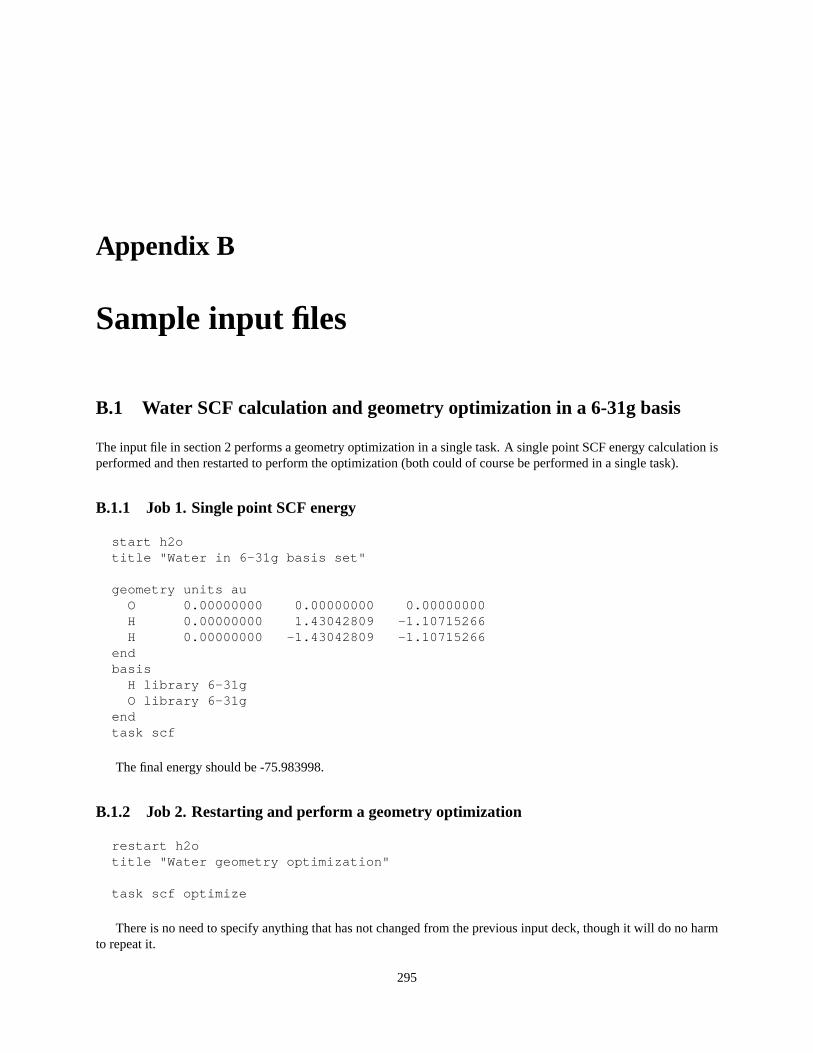
Appendix B
Sample input files
B.1 Water SCF calculation and geometry optimization in a 6-31g basis
The input file in section 2 performs a geometry optimization in a single task. A single point SCF energy calculation isperformed and then restarted to perform the optimization (both could of course be performed in a single task).
B.1.1 Job 1. Single point SCF energy
start h2otitle "Water in 6-31g basis set"
geometry units auO 0.00000000 0.00000000 0.00000000H 0.00000000 1.43042809 -1.10715266H 0.00000000 -1.43042809 -1.10715266
endbasis
H library 6-31gO library 6-31g
endtask scf
The final energy should be -75.983998.
B.1.2 Job 2. Restarting and perform a geometry optimization
restart h2otitle "Water geometry optimization"
task scf optimize
There is no need to specify anything that has not changed from the previous input deck, though it will do no harmto repeat it.
295
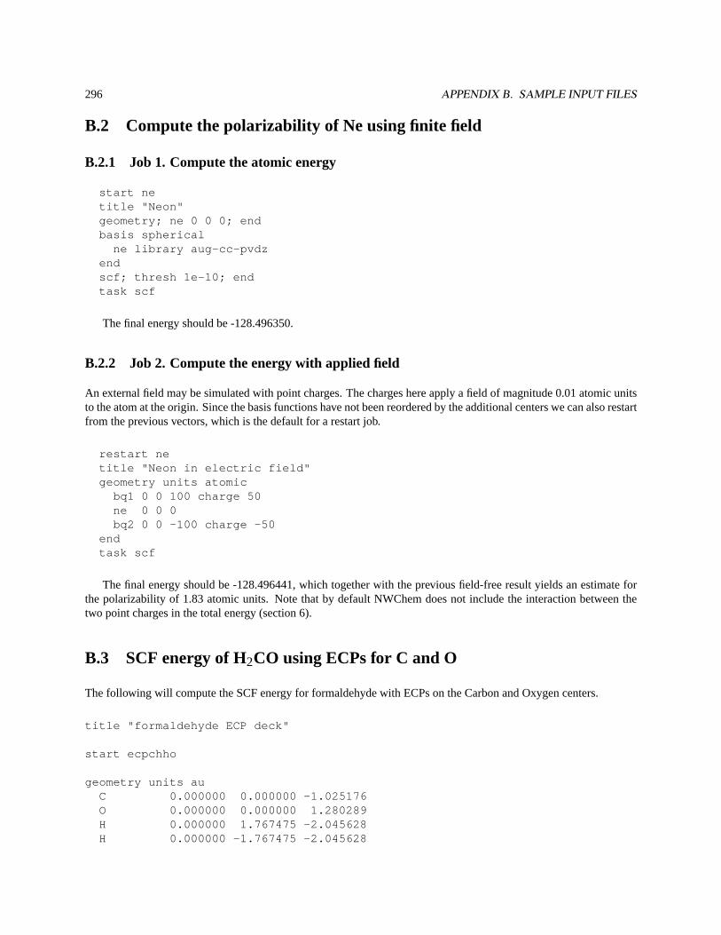
296 APPENDIX B. SAMPLE INPUT FILES
B.2 Compute the polarizability of Ne using finite field
B.2.1 Job 1. Compute the atomic energy
start netitle "Neon"geometry; ne 0 0 0; endbasis spherical
ne library aug-cc-pvdzendscf; thresh 1e-10; endtask scf
The final energy should be -128.496350.
B.2.2 Job 2. Compute the energy with applied field
An external field may be simulated with point charges. The charges here apply a field of magnitude 0.01 atomic unitsto the atom at the origin. Since the basis functions have not been reordered by the additional centers we can also restartfrom the previous vectors, which is the default for a restart job.
restart netitle "Neon in electric field"geometry units atomic
bq1 0 0 100 charge 50ne 0 0 0bq2 0 0 -100 charge -50
endtask scf
The final energy should be -128.496441, which together with the previous field-free result yields an estimate forthe polarizability of 1.83 atomic units. Note that by default NWChem does not include the interaction between thetwo point charges in the total energy (section 6).
B.3 SCF energy of H2CO using ECPs for C and O
The following will compute the SCF energy for formaldehyde with ECPs on the Carbon and Oxygen centers.
title "formaldehyde ECP deck"
start ecpchho
geometry units auC 0.000000 0.000000 -1.025176O 0.000000 0.000000 1.280289H 0.000000 1.767475 -2.045628H 0.000000 -1.767475 -2.045628
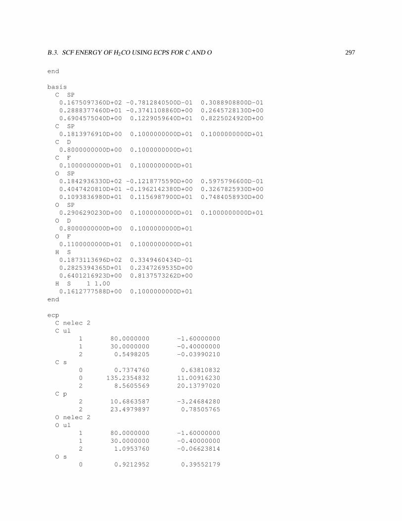
B.3. SCF ENERGY OF H2CO USING ECPS FOR C AND O 297
end
basisC SP
0.1675097360D+02 -0.7812840500D-01 0.3088908800D-010.2888377460D+01 -0.3741108860D+00 0.2645728130D+000.6904575040D+00 0.1229059640D+01 0.8225024920D+00
C SP0.1813976910D+00 0.1000000000D+01 0.1000000000D+01
C D0.8000000000D+00 0.1000000000D+01
C F0.1000000000D+01 0.1000000000D+01
O SP0.1842936330D+02 -0.1218775590D+00 0.5975796600D-010.4047420810D+01 -0.1962142380D+00 0.3267825930D+000.1093836980D+01 0.1156987900D+01 0.7484058930D+00
O SP0.2906290230D+00 0.1000000000D+01 0.1000000000D+01
O D0.8000000000D+00 0.1000000000D+01
O F0.1100000000D+01 0.1000000000D+01
H S0.1873113696D+02 0.3349460434D-010.2825394365D+01 0.2347269535D+000.6401216923D+00 0.8137573262D+00
H S 1 1.000.1612777588D+00 0.1000000000D+01
end
ecpC nelec 2C ul
1 80.0000000 -1.600000001 30.0000000 -0.400000002 0.5498205 -0.03990210
C s0 0.7374760 0.638108320 135.2354832 11.009162302 8.5605569 20.13797020
C p2 10.6863587 -3.246842802 23.4979897 0.78505765
O nelec 2O ul
1 80.0000000 -1.600000001 30.0000000 -0.400000002 1.0953760 -0.06623814
O s0 0.9212952 0.39552179
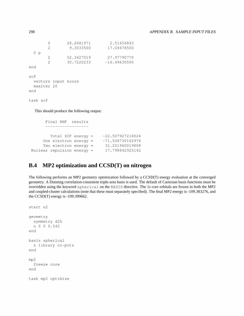
298 APPENDIX B. SAMPLE INPUT FILES
0 28.6481971 2.516548432 9.3033500 17.04478500
O p2 52.3427019 27.977907702 30.7220233 -16.49630500
end
scfvectors input hcoremaxiter 20
end
task scf
This should produce the following output:
Final RHF results------------------
Total SCF energy = -22.507927218024One electron energy = -71.508730162974Two electron energy = 31.201960019808
Nuclear repulsion energy = 17.798842925142
B.4 MP2 optimization and CCSD(T) on nitrogen
The following performs an MP2 geometry optimization followed by a CCSD(T) energy evaluation at the convergedgeometry. A Dunning correlation-consistent triple-zeta basis is used. The default of Cartesian basis functions must beoverridden using the keywordspherical on theBASIS directive. The 1s core orbitals are frozen in both the MP2and coupled-cluster calculations (note that these must separately specified). The final MP2 energy is -109.383276, andthe CCSD(T) energy is -109.399662.
start n2
geometrysymmetry d2hn 0 0 0.542
end
basis sphericaln library cc-pvtz
end
mp2freeze core
end
task mp2 optimize

B.4. MP2 OPTIMIZATION AND CCSD(T) ON NITROGEN 299
ccsdfreeze core
end
task ccsd(t)

300 APPENDIX B. SAMPLE INPUT FILES
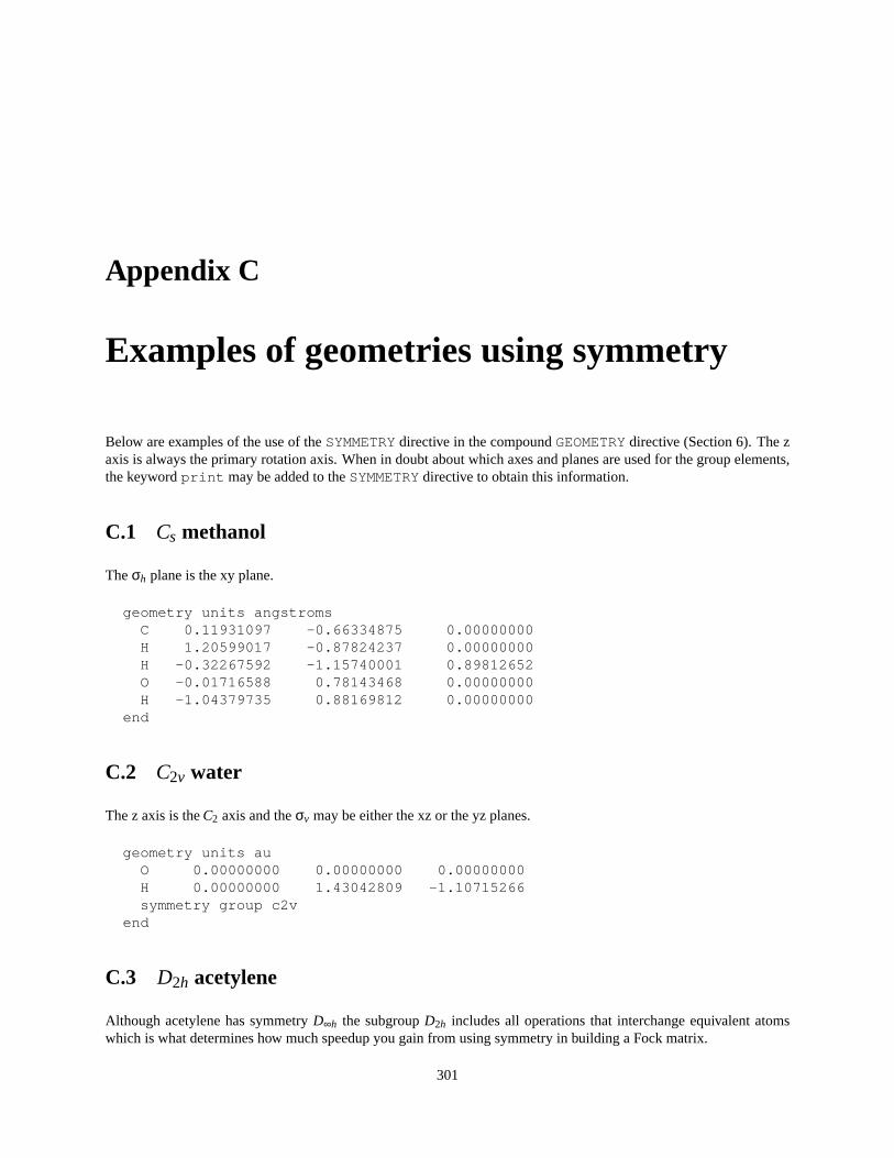
Appendix C
Examples of geometries using symmetry
Below are examples of the use of theSYMMETRYdirective in the compoundGEOMETRYdirective (Section 6). The zaxis is always the primary rotation axis. When in doubt about which axes and planes are used for the group elements,the keywordprint may be added to theSYMMETRYdirective to obtain this information.
C.1 Cs methanol
Theσh plane is the xy plane.
geometry units angstromsC 0.11931097 -0.66334875 0.00000000H 1.20599017 -0.87824237 0.00000000H -0.32267592 -1.15740001 0.89812652O -0.01716588 0.78143468 0.00000000H -1.04379735 0.88169812 0.00000000
end
C.2 C2v water
The z axis is theC2 axis and theσv may be either the xz or the yz planes.
geometry units auO 0.00000000 0.00000000 0.00000000H 0.00000000 1.43042809 -1.10715266symmetry group c2v
end
C.3 D2h acetylene
Although acetylene has symmetryD∞h the subgroupD2h includes all operations that interchange equivalent atomswhich is what determines how much speedup you gain from using symmetry in building a Fock matrix.
301
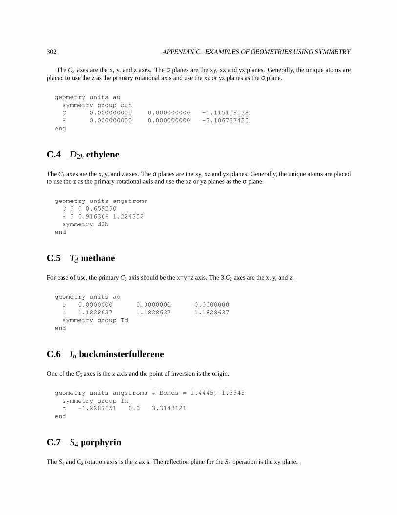
302 APPENDIX C. EXAMPLES OF GEOMETRIES USING SYMMETRY
TheC2 axes are the x, y, and z axes. Theσ planes are the xy, xz and yz planes. Generally, the unique atoms areplaced to use the z as the primary rotational axis and use the xz or yz planes as theσ plane.
geometry units ausymmetry group d2hC 0.000000000 0.000000000 -1.115108538H 0.000000000 0.000000000 -3.106737425
end
C.4 D2h ethylene
TheC2 axes are the x, y, and z axes. Theσ planes are the xy, xz and yz planes. Generally, the unique atoms are placedto use the z as the primary rotational axis and use the xz or yz planes as theσ plane.
geometry units angstromsC 0 0 0.659250H 0 0.916366 1.224352symmetry d2h
end
C.5 Td methane
For ease of use, the primaryC3 axis should be the x=y=z axis. The 3C2 axes are the x, y, and z.
geometry units auc 0.0000000 0.0000000 0.0000000h 1.1828637 1.1828637 1.1828637symmetry group Td
end
C.6 Ih buckminsterfullerene
One of theC5 axes is the z axis and the point of inversion is the origin.
geometry units angstroms # Bonds = 1.4445, 1.3945symmetry group Ihc -1.2287651 0.0 3.3143121
end
C.7 S4 porphyrin
TheS4 andC2 rotation axis is the z axis. The reflection plane for theS4 operation is the xy plane.
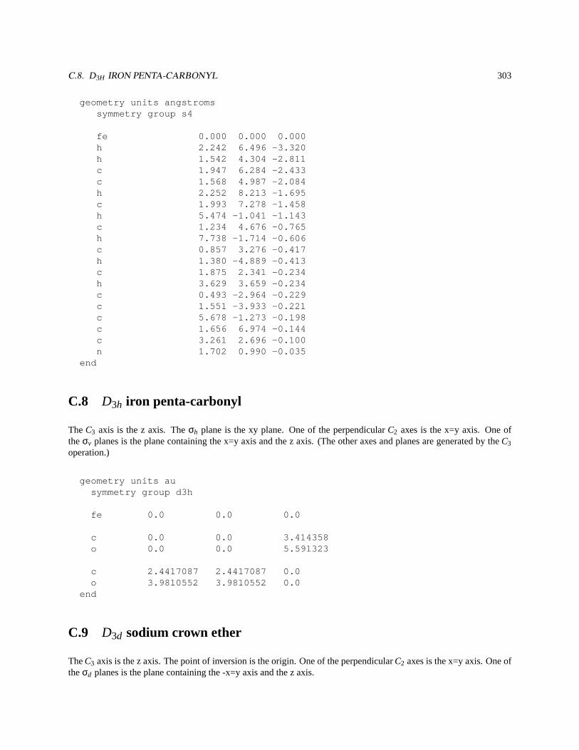
C.8. D3H IRON PENTA-CARBONYL 303
geometry units angstromssymmetry group s4
fe 0.000 0.000 0.000h 2.242 6.496 -3.320h 1.542 4.304 -2.811c 1.947 6.284 -2.433c 1.568 4.987 -2.084h 2.252 8.213 -1.695c 1.993 7.278 -1.458h 5.474 -1.041 -1.143c 1.234 4.676 -0.765h 7.738 -1.714 -0.606c 0.857 3.276 -0.417h 1.380 -4.889 -0.413c 1.875 2.341 -0.234h 3.629 3.659 -0.234c 0.493 -2.964 -0.229c 1.551 -3.933 -0.221c 5.678 -1.273 -0.198c 1.656 6.974 -0.144c 3.261 2.696 -0.100n 1.702 0.990 -0.035
end
C.8 D3h iron penta-carbonyl
TheC3 axis is the z axis. Theσh plane is the xy plane. One of the perpendicularC2 axes is the x=y axis. One oftheσv planes is the plane containing the x=y axis and the z axis. (The other axes and planes are generated by theC3
operation.)
geometry units ausymmetry group d3h
fe 0.0 0.0 0.0
c 0.0 0.0 3.414358o 0.0 0.0 5.591323
c 2.4417087 2.4417087 0.0o 3.9810552 3.9810552 0.0
end
C.9 D3d sodium crown ether
TheC3 axis is the z axis. The point of inversion is the origin. One of the perpendicularC2 axes is the x=y axis. One oftheσd planes is the plane containing the -x=y axis and the z axis.
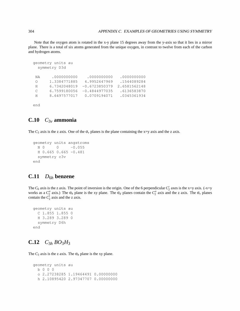
304 APPENDIX C. EXAMPLES OF GEOMETRIES USING SYMMETRY
Note that the oxygen atom is rotated in the x-y plane 15 degrees away from the y-axis so that it lies in a mirrorplane. There is a total of six atoms generated from the unique oxygen, in contrast to twelve from each of the carbonand hydrogen atoms.
geometry units ausymmetry D3d
NA .0000000000 .0000000000 .0000000000O 1.3384771885 4.9952647969 .1544089284H 6.7342048019 -0.6723850379 2.6581562148C 6.7599180056 -0.4844977035 .6136583870H 8.6497577017 0.0709194071 .0345361934
end
C.10 C3v ammonia
TheC3 axis is the z axis. One of theσv planes is the plane containing the x=y axis and the z axis.
geometry units angstromsN 0 0 -0.055H 0.665 0.665 -0.481symmetry c3v
end
C.11 D6h benzene
TheC6 axis is the z axis. The point of inversion is the origin. One of the 6 perpendicularC′2 axes is the x=y axis. (-x=yworks as aC′′2 axis.) Theσh plane is the xy plane. Theσd planes contain theC′′2 axis and the z axis. Theσv planescontain theC′2 axis and the z axis.
geometry units auC 1.855 1.855 0H 3.289 3.289 0symmetry D6h
end
C.12 C3h BO3H3
TheC3 axis is the z axis. Theσh plane is the xy plane.
geometry units aub 0 0 0o 2.27238285 1.19464491 0.00000000h 2.10895420 2.97347707 0.00000000
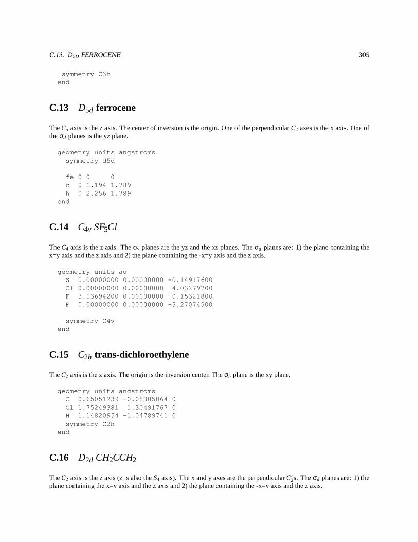
C.13. D5D FERROCENE 305
symmetry C3hend
C.13 D5d ferrocene
TheC5 axis is the z axis. The center of inversion is the origin. One of the perpendicularC2 axes is the x axis. One oftheσd planes is the yz plane.
geometry units angstromssymmetry d5d
fe 0 0 0c 0 1.194 1.789h 0 2.256 1.789
end
C.14 C4v SF5Cl
TheC4 axis is the z axis. Theσv planes are the yz and the xz planes. Theσd planes are: 1) the plane containing thex=y axis and the z axis and 2) the plane containing the -x=y axis and the z axis.
geometry units auS 0.00000000 0.00000000 -0.14917600Cl 0.00000000 0.00000000 4.03279700F 3.13694200 0.00000000 -0.15321800F 0.00000000 0.00000000 -3.27074500
symmetry C4vend
C.15 C2h trans-dichloroethylene
TheC2 axis is the z axis. The origin is the inversion center. Theσh plane is the xy plane.
geometry units angstromsC 0.65051239 -0.08305064 0Cl 1.75249381 1.30491767 0H 1.14820954 -1.04789741 0symmetry C2h
end
C.16 D2d CH2CCH2
TheC2 axis is the z axis (z is also theS4 axis). The x and y axes are the perpendicularC′2s. Theσd planes are: 1) theplane containing the x=y axis and the z axis and 2) the plane containing the -x=y axis and the z axis.
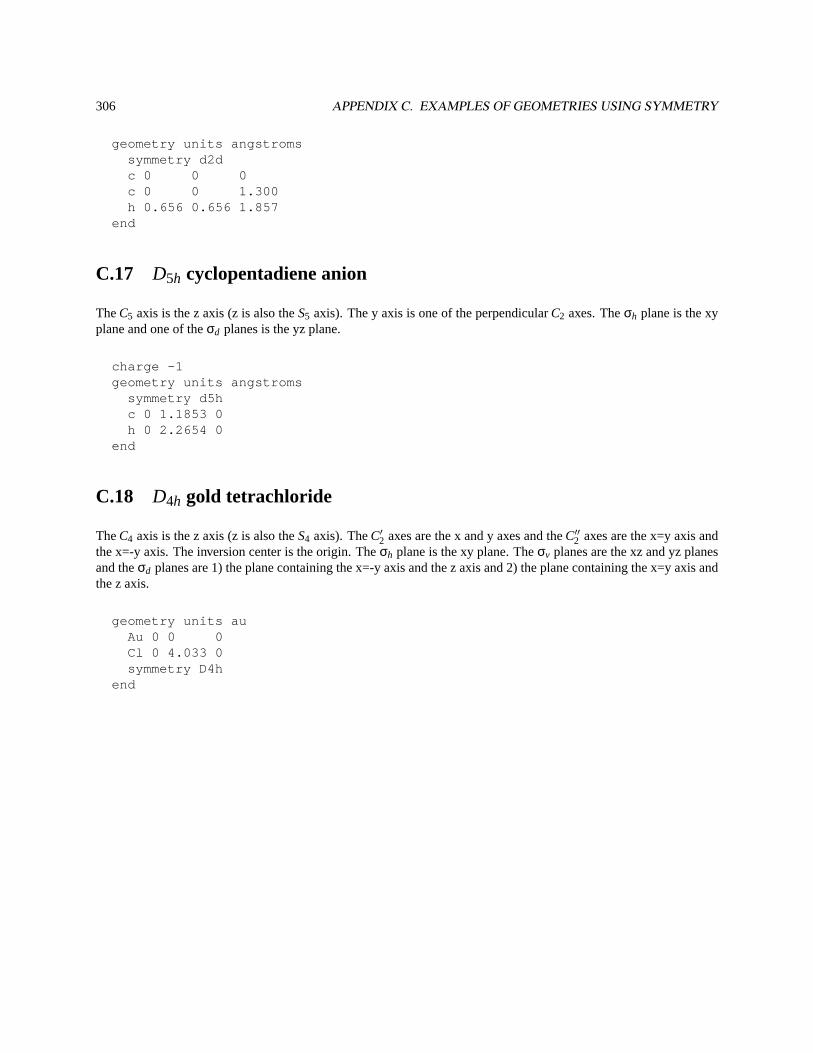
306 APPENDIX C. EXAMPLES OF GEOMETRIES USING SYMMETRY
geometry units angstromssymmetry d2dc 0 0 0c 0 0 1.300h 0.656 0.656 1.857
end
C.17 D5h cyclopentadiene anion
TheC5 axis is the z axis (z is also theS5 axis). The y axis is one of the perpendicularC2 axes. Theσh plane is the xyplane and one of theσd planes is the yz plane.
charge -1geometry units angstroms
symmetry d5hc 0 1.1853 0h 0 2.2654 0
end
C.18 D4h gold tetrachloride
TheC4 axis is the z axis (z is also theS4 axis). TheC′2 axes are the x and y axes and theC′′2 axes are the x=y axis andthe x=-y axis. The inversion center is the origin. Theσh plane is the xy plane. Theσv planes are the xz and yz planesand theσd planes are 1) the plane containing the x=-y axis and the z axis and 2) the plane containing the x=y axis andthe z axis.
geometry units auAu 0 0 0Cl 0 4.033 0symmetry D4h
end
Appendix D
Running NWChem
The command required to invoke NWChem is machine dependent, whereas most of the NWChem input is machineindependent1 .
D.1 Sequential execution
To run NWChem sequentially on nearly all UNIX-based platforms simply use the commandnwchemand provide thename of the input file as an argument (See section 2.1 for more information). This does assume that eithernwchem isin your path or you have set an alias ofnwchem to point to the appropriate executable.
Output is to standard output, standard error and Fortran unit 6 (usually the same as standard output). Files arecreated by default in the current directory, though this may be overridden in the input (section 5.2).
Generally, one will run a job with the following command:
nwchem input.nw >& input.out &
D.2 Parallel execution on UNIX-based parallel machines including work-station clusters using TCGMSG
These platforms require the use of the TCGMSG2 parallel command and thus also require the definition of aprocess-group (or procgroup) file. The process-group file describes how many processes to start, what program to run,which machines to use, which directories to work in, and under which userid to run the processes. By convention theprocess-group file has a.p suffix.
The process-group file is read to end-of-file. The character# (hash or pound sign) is used to indicate a commentwhich continues to the next new-line character. Each line describes a cluster of processes and consists of the followingwhitespace separated fields:
userid hostname nslave executable workdir
1Machine dependence within the input arises from file names, machine specific resources, and differing services provided by the operatingsystem.
2Where required TCGMSG is automatically built with NWChem.
307
308 APPENDIX D. RUNNING NWCHEM
• userid – The user-name on the machine that will be executing the process.
• hostname – The hostname of the machine to execute this process. If it is the same machine on which parallelwas invoked the name must match the value returned by the command hostname. If a remote machine it mustallow remote execution from this machine (see man pages for rlogin, rsh).
• nslave – The total number of copies of this process to be executing on the specified machine. Only “clusters”of identical processes specified in this fashion can use shared memory to communicate. If no shared memory issupported on machine<hostname> then only the value one (1) is valid.
• executable – Full path name on the host<hostname> of the image to execute. If<hostname> is thelocal machine then a local path will suffice.
• workdir – Full path name on the host<hostname> of the directory to work in. Processes execute a chdir()to this directory before returning from pbegin(). If specified as a “.” then remote processes will use the logindirectory on that machine and local processes (relative to where parallel was invoked) will use the currentdirectory of parallel.
For example, if your file"nwchem.p" contained the following
d3g681 pc 4 /msrc/apps/bin/nwchem /scr22/rjh
then 4 processes running NWChem would be started on the machinepc running as userd3g681 in directory"/scr22/rjh" . To actually run this simply type:
parallel nwchem big_molecule.nw
N.B.: The first process specified (process zero) is the only process that
• opens and reads the input file, and
• opens and reads/updates the database.
Thus, if your file systems are physically distributed (e.g., most workstation clusters) you must ensure that process zerocan correctly resolve the paths for the input and database files.
N.B.In releases of NWChem prior to 3.3 additional processes had to be created on workstation clusters to supportremote access to shared memory. This is no longer the case. The TCGMSG process group file now just needs to referto processes running NWChem.
D.3 Parallel execution on UNIX-based parallel machines including work-station clusters using MPI
To run with MPI,parallel should not be used. The way we usually run nwchem under MPI are the following
• using mpirun:
mpirun -np 8 $NWCHEM_TOP/bin/$NWCHEM_TARGET/nwchem input.nw
• If you have all nodes connected via shared memory and you have installed the ch_shmem version of MPICH,you can do
$NWCHEM_TOP/bin/$NWCHEM_TARGET/nwchem -np 8 h2o.nw
D.4. PARALLEL EXECUTION ON MPPS 309
D.4 Parallel execution on MPPs
All of these machines require use of different commands in order to gain exclusive access to computational resources.
D.5 IBM SP
If using POE (IBM’s Parallel Operating Environment) interactively, simply create the list of nodes to use in the file"host.list" in the current directory and invoke NWChem with
nwchem <input_file> -procs <n>
wheren is the number of processes to use. Process 0 will run on the first node in"host.list" and must haveaccess to the input and other necessary files. Very significant performance gains may be had by setting the followingenvironment variables before running NWChem (or setting them using POE command line options).
• setenv MP_EUILIB us — dedicated user space communication over the switch (the default is IP over theswitch which is much slower).
• setenv MP_CSS_INTERRUPT yes — enable interrupts when a message arrives (the default is to pollwhich significantly slows down global array accesses).
In addition, if the IBM is running PSSP version 3.1, or later
• setenv MP_MSG_API lapi , or
• setenv MP_MSG_API mpi,lapi (if using both GA and MPI)
For batch execution, we recommend use of thellnw command which is installed in/usr/local/bin on theEMSL/PNNL IBM SP. If you are not running on that system, thellnw script may be found in the NWChem distribu-tion directory contrib/loadleveler. Interactive help may be obtained with the commandllnw -help . Otherwise, thevery simplest job to run NWChem in batch using Load Leveller is something like this
#!/bin/csh -x# @ job_type = parallel# @ class = small# @ network.lapi = css0,not_shared,US# @ input = /dev/null# @ output = <OUTPUT_FILE_NAME># @ error = <ERROUT_FILE_NAME># @ environment = COPY_ALL; MP_PULSE=0; MP_SINGLE_THREAD=yes; MP_WAIT_MODE=yield; restart=no# @ min_processors = 7# @ max_processors = 7# @ cpu_limit = 1:00:00# @ wall_clock_limit = 1:00:00# @ queue#
cd /scratch
nwchem <INPUT_FILE_NAME>
310 APPENDIX D. RUNNING NWCHEM
Substitute<OUTPUT_FILE_NAME>, <ERROUT_FILE_NAME>and<INPUT_FILE_NAME> with thefull pathof the appropriate files. Also, if you are using an SP with more than one processor per node, you will need to substitute
# @ network.lapi = css0,shared,US# @ node = NNODE# @ tasks_per_node = NTASK
for the lines
# @ network.lapi = css0,not_shared,US# @ min_processors = 7# @ max_processors = 7
whereNNODEis the number of physical nodes to be used andNTASKis the number of tasks per node.
These files and the NWChem executable must be in a file system accessible to all processes. Put the above into afile (e.g.,"test.job" ) and submit it with the command
llsubmit test.job
It will run a 7 processor, 1 hour job in the queuesmall . It should be apparent how to change these values.
Note that on many IBM SPs, including that at EMSL, the local scratch disks are wiped clean at the beginning ofeach job and therefore persistent files should be stored elsewhere. PIOFS is recommended for files larger than a fewMB.
D.6 Cray T3E
mpprun -n <npes> $NWCHEM_TOP/bin/$NWCHEM_TARGET/nwchem <input_file>
wherenpes is the number of processors andinput_file is the name of your input file.
D.7 Linux
If running in parallel across multiple machines you should consider applying this patch to your kernel to boost theperformance of TCP/IP
• http://www.icase.edu/coral/LinuxTCP.html
D.8 Alpha systems with Quadrics switch
prun -n <npes> $NWCHEM_TOP/bin/$NWCHEM_TARGET/nwchem <input_file>
wherenpes is the number of processors andinput_file is the name of your input file.
D.9. WINDOWS 98 AND NT 311
D.9 Windows 98 and NT
$NWCHEM_TOP/bin/win32/nw32 <input_file>
where andinput_file is the name of your input file. If you use WMPI, uou must have a file namednw32.pgin the $NWCHEM_TOP/bin/win32 directory; the file must only contains the following single line
local 0
D.10 Tested Platforms and O/S versions
• IBM SP with P2SC nodes, AIX 4.2.1, and PSSP 2.3
• IBM SP with silver nodes (SMP nodes with two 604e processors), AIX 4.3.2, and PSSP 3.1.
• IBM RS6000 workstation, AIX 3.2 and 4.1.
• Cray T3E, 2.0.4.61 UNICOSMK
• SGI R8000/10000, IRIX 6.2, 6.5
• SGI R4000, IRIX 5.3
• SUN workstations, SunOS 4.1.3 and Solaris 5.5, 5.6
• Compaq DEC alpha workstion
– (600 MHz EV6), Digital UNIX V4.0E Rev. 1091, DEC C V5.8-009, Digital Fortran V5.2
– (667 MHz EV6), Digital UNIX V4.0F Rev. 1229, DEC C V5.9-005, Digital Fortran V5.2
• Linux. Since there are at least 8 popular distributions of the Linux operating system and numerous othersin existence, including downloading everything and building your own Linux OS, it is impossible to test allpossible versions of Linux with NWChem. NWChem Release 3.3 has been tested on Slackware 3.4, 3.5, 4.0,7.0 RedHat 5.1, 5.2, and 6.0, 6.1, 6.2 Mandrake based on RedHat 6.0, RedHat 6.0 for the Power PC Macintosh,and Black Lab 1.2 or Yellow Dog 1.2 Linux for Power PC Macintosh. These all use the EGCS compilers atdifferent levels. Those distributed from Slackware are somewhat different than those distributed from RedHatbut the code is configured to run on all of them.
• Linux on Alpha cpus has been tested with RedHat 6.1 and 6.2. Usage of the Compaq Fortran and C compilersis necessary for compiling.
• HP 9000/800 workstations with HPUX B.11.00. f90 must be used for compilation.
• FreeBSD. Just use the Linux target and NWChem will build for FreeBSD version 4.0 and the pre-release 5.0versions of the Operating System.
• Intel x86 with Windows 98 and NT has been tested with Compaq Visual Fortran 6.0 and 6.1 with WMPI 1.3 orNT-MPICH. NT-MPICH is available from http://www-unix.mcs.anl.gov/˜ashton/mpich.nt/


![Scaling NWChem with Efficient and Portable Asynchronous Communication in MPI RMA Min Si [1][2], Antonio J. Peña [1], Jeff Hammond [3], Pavan Balaji [1],](https://img.pdfslide.us/doc/110x75/56649f395503460f94c55ce4/scaling-nwchem-with-efficient-and-portable-asynchronous-communication-in-mpi.jpg)