INTER-NOISE 2007

28-31 AUGUST 2007 ISTANBUL, TURKEY

NVH tools and methods for sound design of vehicles

Roland Sotteka and Bernhard Müller-Heldb

HEAD acoustics GmbH

Ebertstr. 30a D-52134 Herzogenrath

GERMANY

ABSTRACT Interior vehicle sound is an important factor for customer satisfaction. Thus, Binaural Transfer Path Analysis and Synthesis (BTPA/BTPS) have been developed for troubleshooting and sound design of engine-related vehicle interior noise. These methods allow not only the prediction of order levels and spectra, but also the binaural auralization of various driving conditions, as well as the prediction of vibrations such as at the driver’s seat and steering wheel. With the help of the BTPA/BTPS methods engineers can distinguish between the excitation source and the transfer behavior of individual elements, and can therefore more precisely identify the cause of a particular disturbing noise pattern. Recent extensions of the methods allow predicting the impact of particular structure-borne transfer paths with the help of four-pole parameters, measured on a test-rig or calculated by Finite Element Analysis (FEA). The simulated transfer paths can be substituted for the original measured paths in the BTPS model. The next step in the sound design process is an adequate characterization of excitation sources, with respect to source strength and source impedance under running conditions. This paper will introduce an extended approach allowing for an improved consideration of the coupling between different subsystems.

1 INTRODUCTION Binaural Transfer Path Analysis and Synthesis (BTPA/BTPS) are well-known tools for

troubleshooting and sound design of vehicle interior noise [1]. Frequently, the combustion engine in combination with intake and exhaust systems (power train) are, for various driving conditions, the dominant noise sources with respect to interior noise. BTPA/BTPS enable exploring the causative mechanisms for noise transfers, based on measurements of excitation source strengths and the corresponding structure-borne and airborne transfer paths to a receiver position (e.g., the driver position). The results of these tools represent a considerable milestone with respect to acoustic simulation and auralization. The engineer can analyze and listen not only to the overall sound comparable to a binaural recording of the vehicle interior sound, but also to components of the total noise transmitted via a single path or a combination of paths to identify the cause of a particular disturbing noise pattern.

The next step in a sound design process includes modifying noise and vibration sources and/or transfer paths. The improvements of BTPA and BTPS based on the system-theoretical method of four-pole theory allow simulating the combination of different subsystems and enable the physically correct description of structure-borne transmission under different load

a Email address: Roland.Sottek@HEAD-acoustics.de b Email address: Bernhard.Mueller-Held@HEAD-acoustics.de

conditions of the engine (test rig or vehicle measurements). Using these recently-developed techniques, a significant reduction of laborious measurements with repeatedly-reconstructed vehicle prototypes is achievable [2], [3].

At present, the application of Finite Element Analysis (FEA) for calculating the four-pole parameters helps in predicting the impact of particular structure-borne transfer paths. The simulated transfer paths can be substituted for the original measured paths in the BTPS-model. This approach offers new sound design possibilities by virtually changing the geometry (e.g., shape, wall thicknesses) and/or material properties. The effects of the modifications on the vehicle interior sound can be analyzed and subjectively evaluated during listening tests, even in the early design phase [4].

It must be pointed out that modifying a specific transfer path like an engine mount may also influence the source signals, in this case the vibration signals at the engine side of the mount. This fact is often neglected. The vibration signals will be changed if the engine is connected to a different mount and/or to a different structure, like the body of a vehicle or an engine test-rig. Therefore, the sound design process requires an adequate description of excitation sources. This paper will introduce improved BTPA/BTPS methods using a source characterization with respect to source strength and source impedance under running conditions. The resulting source description does not depend on the connected subsystems. The vibration signals for a specific load condition can be calculated easily, based on the source parameters and the load impedance of the connected system.

For demonstration purposes, the described methods are applied to a small vehicle simulator with reduced complexity. This model allows for fast structural changes, and its operation is also very flexible with respect to source strength modifications. The results of the measurements and simulations will be presented. It should be noted that in the case of the vehicle simulator only a monaural receiver (a microphone, due to space limitations) is applied, whereas in a real car normally an artificial head records the sound in an aurally-adequate way. Nevertheless, the terminology BTPA/BTPS is still used for the vehicle simulator.

2 VEHICLE SIMULATOR FOR BTPA/BTPS DEMONSTRATION

shaker

mount

cabin loudspeaker

body

microphone

xy

z

shaker

mount

cabin loudspeaker

body

microphone

xy

z

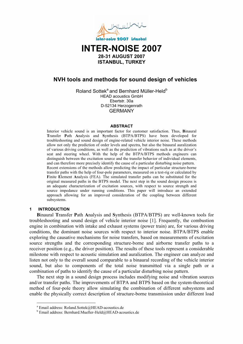
Figure 1: Vehicle simulator

In Figure 1 a small vehicle simulator is shown. A body is placed with three mounts on a soft, damped base plate to prevent external disturbances. On one side a cabin with Plexiglas® is attached. Inside the cabin is a microphone, representing the driver’s ear. On the other side of the body are two sources which together represent an engine. A shaker mainly produces structure-borne noise. It is fixed to a beam which is screwed with one mount to the body. A loudspeaker produces mainly airborne noise. This vehicle simulator has accordance to a real

vehicle in that a cabin is coupled over a chassis, and an engine mount to the engine. In addition, the airborne transfer path of the engine is considered.

3 OVERVIEW OF BTPA/BTPS The challenge of the BTPA/BTPS methods is to break down a complex noise into its

components. Therefore all acoustically-relevant airborne and structure-borne sources must be detected and considered in the BTPS model. These sources are linked to airborne and structure-borne paths which will be introduced in the next paragraphs.

3.1 Airborne Transfer Path The airborne transfer paths are the transfer functions between the volume flow of the

sources and the acoustic pressure measured at the receiver position. In reciprocal measurements the positions of transmitter (source) and receiver (sensor) are interchanged. Using the reciprocity principle, all the transfer paths are determined within one measurement: the exciting sound source at the receiver position is fed with a sweep signal, and the radiated sound is recorded simultaneously by all component microphones in the near field of the assumed real sound sources.

Synthesizing the airborne contributions demands volume flow as the input signal. Whereas normally the volume flow of the exciting source used for transfer function measurements is known, determining the volume flow of real sources like an engine is difficult [3]. Thus instead the sound pressure in the vicinity of the assumed sources is often taken as input signal. The corresponding airborne transfer functions are measured by relating the microphone signal at the receiver position with the microphone signals at the source position while exciting in each case with a loudspeaker in the vicinity of the assumed sources. This approach requires adequate consideration of crosstalk between different sources and measurement positions.

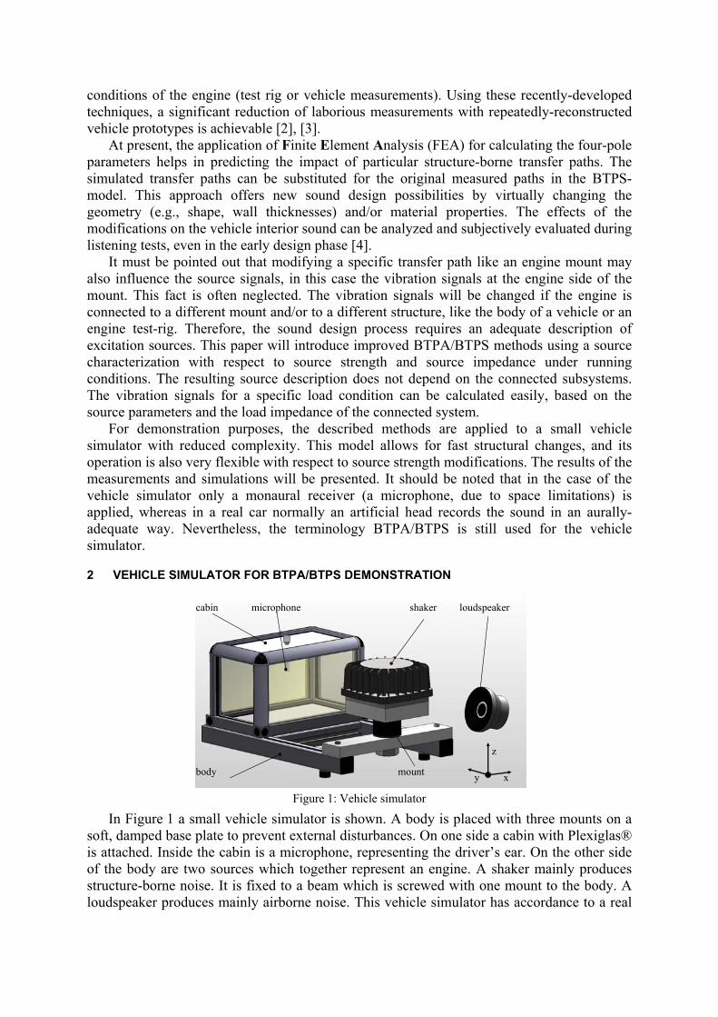
The simplified vehicle simulator has only one airborne sound source: a loudspeaker. The loudspeaker itself is excited with a sweep signal, and the sound pressure signals in the cabin and in front of the speaker are measured simultaneously in order to determine the airborne transfer function ATF

AB by correlation analyses (Figure 2).

enginep

t

ABATFABreceiverp

Sweep excitation

Figure 2: Airborne transfer path measurement

In real cars, the airborne sources can be found at different positions in the engine compartment, at the intake system, and at the exhaust pipe. To determine the corresponding transfer functions the sound pressure is measured at both ears of an artificial head placed on the driver’s seat while exciting with a single loudspeaker close to each assumed source.

3.2 Structure-Borne Transfer Path Each structure-borne transfer path from the source (engine side of the mounts) to the

receiver position (microphone in the cabin, and at the driver’s ears respectively in a real vehicle) can be described using two transfer functions, one after another: the mount transfer function MTF and the acoustical transfer function ATF

SB. The mount transfer function is the ratio of the force at the body side to the velocity at the engine side Fbody/vbody and the acoustical transfer function is the ratio of the sound pressure at the receiver position (e.g., at the driver’s ears) to the force at the body side.

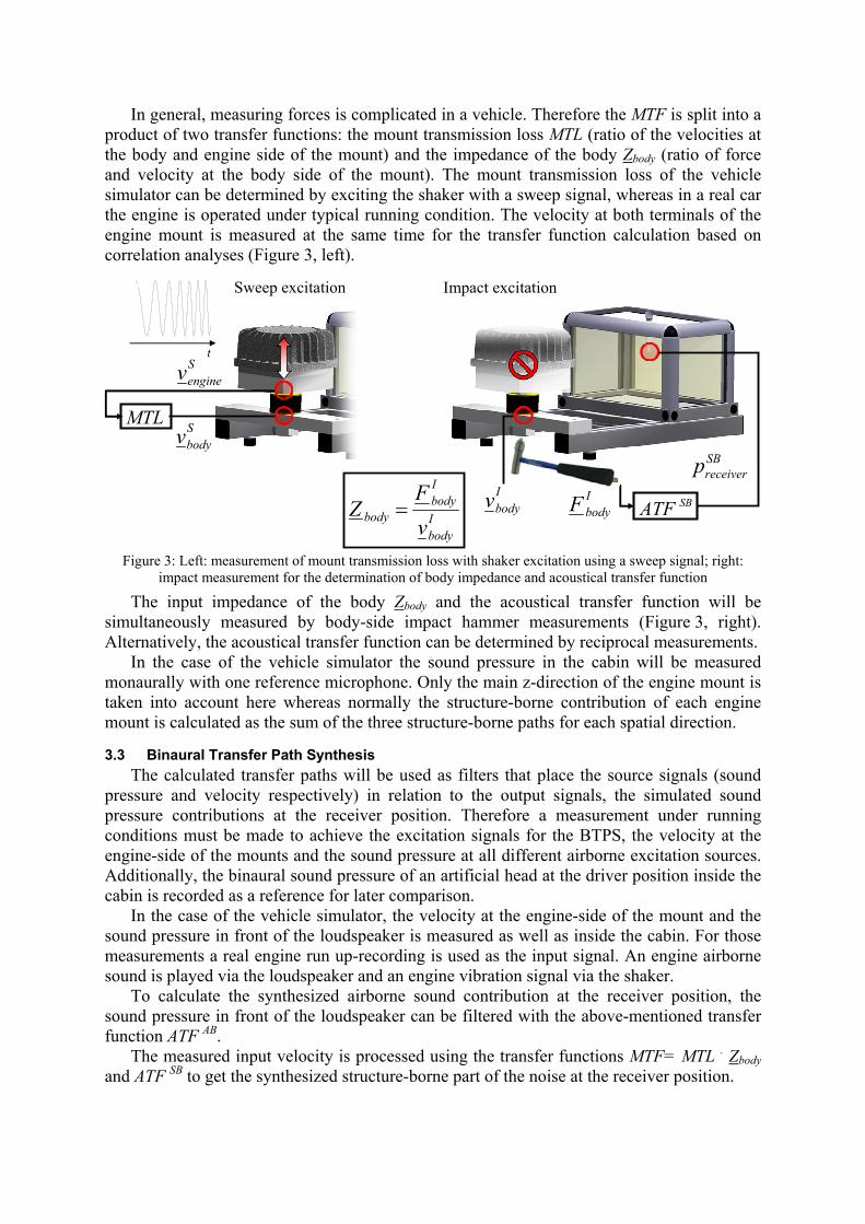
In general, measuring forces is complicated in a vehicle. Therefore the MTF is split into a product of two transfer functions: the mount transmission loss MTL (ratio of the velocities at the body and engine side of the mount) and the impedance of the body Zbody (ratio of force and velocity at the body side of the mount). The mount transmission loss of the vehicle simulator can be determined by exciting the shaker with a sweep signal, whereas in a real car the engine is operated under typical running condition. The velocity at both terminals of the engine mount is measured at the same time for the transfer function calculation based on correlation analyses (Figure 3, left).

MTL

Senginev

Sbodyv

Sweep excitation

t

Impact excitation

Ibodyv I

bodyF

SBreceiverp

SBATFIbody

Ibody

body vF

Z =

Figure 3: Left: measurement of mount transmission loss with shaker excitation using a sweep signal; right: impact measurement for the determination of body impedance and acoustical transfer function

The input impedance of the body Zbody and the acoustical transfer function will be simultaneously measured by body-side impact hammer measurements (Figure 3, right). Alternatively, the acoustical transfer function can be determined by reciprocal measurements.

In the case of the vehicle simulator the sound pressure in the cabin will be measured monaurally with one reference microphone. Only the main z-direction of the engine mount is taken into account here whereas normally the structure-borne contribution of each engine mount is calculated as the sum of the three structure-borne paths for each spatial direction.

3.3 Binaural Transfer Path Synthesis The calculated transfer paths will be used as filters that place the source signals (sound

pressure and velocity respectively) in relation to the output signals, the simulated sound pressure contributions at the receiver position. Therefore a measurement under running conditions must be made to achieve the excitation signals for the BTPS, the velocity at the engine-side of the mounts and the sound pressure at all different airborne excitation sources. Additionally, the binaural sound pressure of an artificial head at the driver position inside the cabin is recorded as a reference for later comparison.

In the case of the vehicle simulator, the velocity at the engine-side of the mount and the sound pressure in front of the loudspeaker is measured as well as inside the cabin. For those measurements a real engine run up-recording is used as the input signal. An engine airborne sound is played via the loudspeaker and an engine vibration signal via the shaker.

To calculate the synthesized airborne sound contribution at the receiver position, the sound pressure in front of the loudspeaker can be filtered with the above-mentioned transfer function ATF AB.

The measured input velocity is processed using the transfer functions MTF= MTL . Zbody and ATF SB to get the synthesized structure-borne part of the noise at the receiver position.

engine run ups

enginep

enginevreferencep

SBdsynthesizep

ABdsynthesizepABATF

SBATFMTF

SBABdsynthesizep +

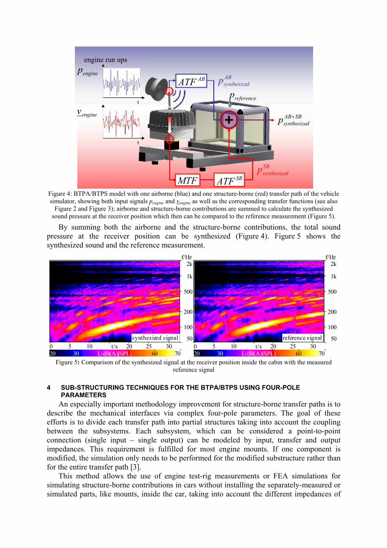
Figure 4: BTPA/BTPS model with one airborne (blue) and one structure-borne (red) transfer path of the vehicle simulator, showing both input signals pengine and vengine as well as the corresponding transfer functions (see also

Figure 2 and Figure 3); airborne and structure-borne contributions are summed to calculate the synthesized sound pressure at the receiver position which then can be compared to the reference measurement (Figure 5).

By summing both the airborne and the structure-borne contributions, the total sound pressure at the receiver position can be synthesized (Figure 4). Figure 5 shows the synthesized sound and the reference measurement.

BTPS Modell 2_synthesized signal alles synhese.FF f/Hz

50

100

200

500

1k

2k

t/s0 5 10 20 25 30L/dB(A)[SPL]20 30 60 70

synthesized signal

BTPS Modell 2_reference signal.FFT vs. Time (1024, f/Hz

50

100

200

500

1k

2k

t/s0 5 10 20 25 30L/dB(A)[SPL]20 30 60 70

reference signal

Figure 5: Comparison of the synthesized signal at the receiver position inside the cabin with the measured

reference signal

4 SUB-STRUCTURING TECHNIQUES FOR THE BTPA/BTPS USING FOUR-POLE PARAMETERS

An especially important methodology improvement for structure-borne transfer paths is to describe the mechanical interfaces via complex four-pole parameters. The goal of these efforts is to divide each transfer path into partial structures taking into account the coupling between the subsystems. Each subsystem, which can be considered a point-to-point connection (single input – single output) can be modeled by input, transfer and output impedances. This requirement is fulfilled for most engine mounts. If one component is modified, the simulation only needs to be performed for the modified substructure rather than for the entire transfer path [3].

This method allows the use of engine test-rig measurements or FEA simulations for simulating structure-borne contributions in cars without installing the separately-measured or simulated parts, like mounts, inside the car, taking into account the different impedances of

body and test-rig. The description of a component using four-pole parameters is independent of the load. Knowing the impedances of the car at the engine mount positions (engine and body side) and the four-pole parameters of the engine mount, a complete simulation of the signal transmission from engine to body and finally to the driver’s ears can be carried out. Any combination of test-rig, FEA- and vehicle data is possible.

softsoft stiffstiffmediummedium

Engine impedance

SZ Z

Four-pole Load impedance

1v 2v1F 2F

bodyZ

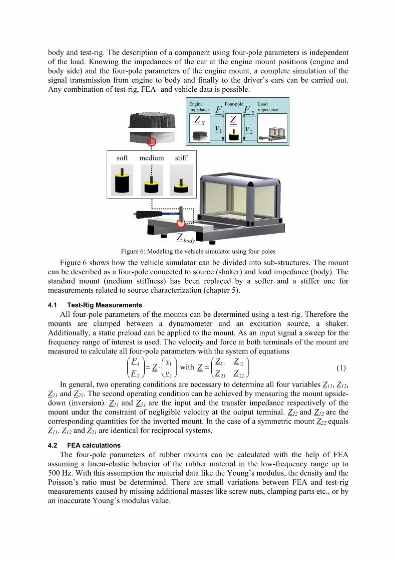
Figure 6: Modeling the vehicle simulator using four-poles

Figure 6 shows how the vehicle simulator can be divided into sub-structures. The mount can be described as a four-pole connected to source (shaker) and load impedance (body). The standard mount (medium stiffness) has been replaced by a softer and a stiffer one for measurements related to source characterization (chapter 5).

4.1 Test-Rig Measurements All four-pole parameters of the mounts can be determined using a test-rig. Therefore the

mounts are clamped between a dynamometer and an excitation source, a shaker. Additionally, a static preload can be applied to the mount. As an input signal a sweep for the frequency range of interest is used. The velocity and force at both terminals of the mount are measured to calculate all four-pole parameters with the system of equations

⎟⎟⎠

⎞⎜⎜⎝

⎛⋅=⎟⎟

⎠

⎞⎜⎜⎝

⎛

2

1

2

1

vv

ZFF

with ⎟⎟⎠

⎞⎜⎜⎝

⎛=

2221

1211

ZZZZ

Z (1)

In general, two operating conditions are necessary to determine all four variables Z11, Z12, Z21 and Z22. The second operating condition can be achieved by measuring the mount upside-down (inversion). Z11 and Z21 are the input and the transfer impedance respectively of the mount under the constraint of negligible velocity at the output terminal. Z22 and Z12 are the corresponding quantities for the inverted mount. In the case of a symmetric mount Z22 equals Z11. Z12 and Z21 are identical for reciprocal systems.

4.2 FEA calculations The four-pole parameters of rubber mounts can be calculated with the help of FEA

assuming a linear-elastic behavior of the rubber material in the low-frequency range up to 500 Hz. With this assumption the material data like the Young’s modulus, the density and the Poisson’s ratio must be determined. There are small variations between FEA and test-rig measurements caused by missing additional masses like screw nuts, clamping parts etc., or by an inaccurate Young’s modulus value.

A fitting algorithm allows for adapting the Young’s modulus, the damping coefficient and the additional mass. Based on comparing the FEA calculation with the test-rig measurements for one spatial direction (the longitudinal direction which is normally easier to operate), all parameters and boundary conditions of the FEA-model are corrected. Then, just by changing the direction of the input load, the reaction forces and deformations affected by this new boundary condition can be recalculated in order to obtain the four-pole parameters for the other spatial directions without further laborious test-rig measurements [4].

4.3 Integration of the four-pole parameters into the BTPS model The previous paragraph described how to determine the mount transfer function for

infinite load impedance, i.e., Z21 (vanishing velocity at the body side of the mount). If the mount is coupled to any known load impedance the resulting ratio of force at the body side to velocity at the engine side can be calculated using the four-pole parameters from the FEA simulation and/or the test-rig results:

bodyZZ

ZvF

22

21

1

2

1+= .

(2)

For example in a car, the load impedance Zbody can be determined by performing an impact hammer measurement at the body side of the engine mount (Figure 6). All necessary load impedances can be determined, measuring in all three directions in space.

5 SOURCE CHARACTERIZATION The use of four-pole parameters for characterizing engine mounts offers new possibilities

of sound design by virtually exchanging mounts, without having to perform any installations in the car. Equation (2) is needed to calculate the force at the body side based on some four-pole parameters and the body impedance in dependence of the velocity at the engine side. But in general it must be taken into account that the strength of the excitation source is also affected by the engine-mount-chassis fixture and the engine impedance.

~

SZSv

Sv

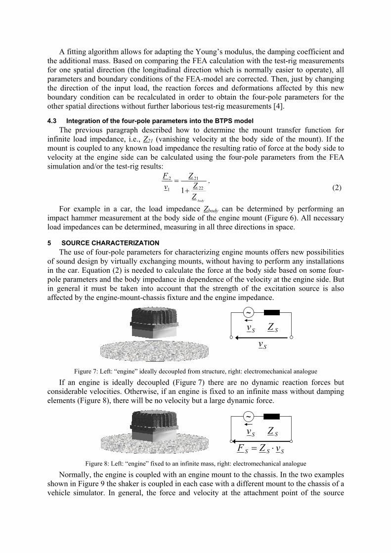
Figure 7: Left: “engine” ideally decoupled from structure, right: electromechanical analogue

If an engine is ideally decoupled (Figure 7) there are no dynamic reaction forces but considerable velocities. Otherwise, if an engine is fixed to an infinite mass without damping elements (Figure 8), there will be no velocity but a large dynamic force.

~

SZSv

SSS vZF ⋅=

Figure 8: Left: “engine” fixed to an infinite mass, right: electromechanical analogue

Normally, the engine is coupled with an engine mount to the chassis. In the two examples shown in Figure 9 the shaker is coupled in each case with a different mount to the chassis of a vehicle simulator. In general, the force and velocity at the attachment point of the source

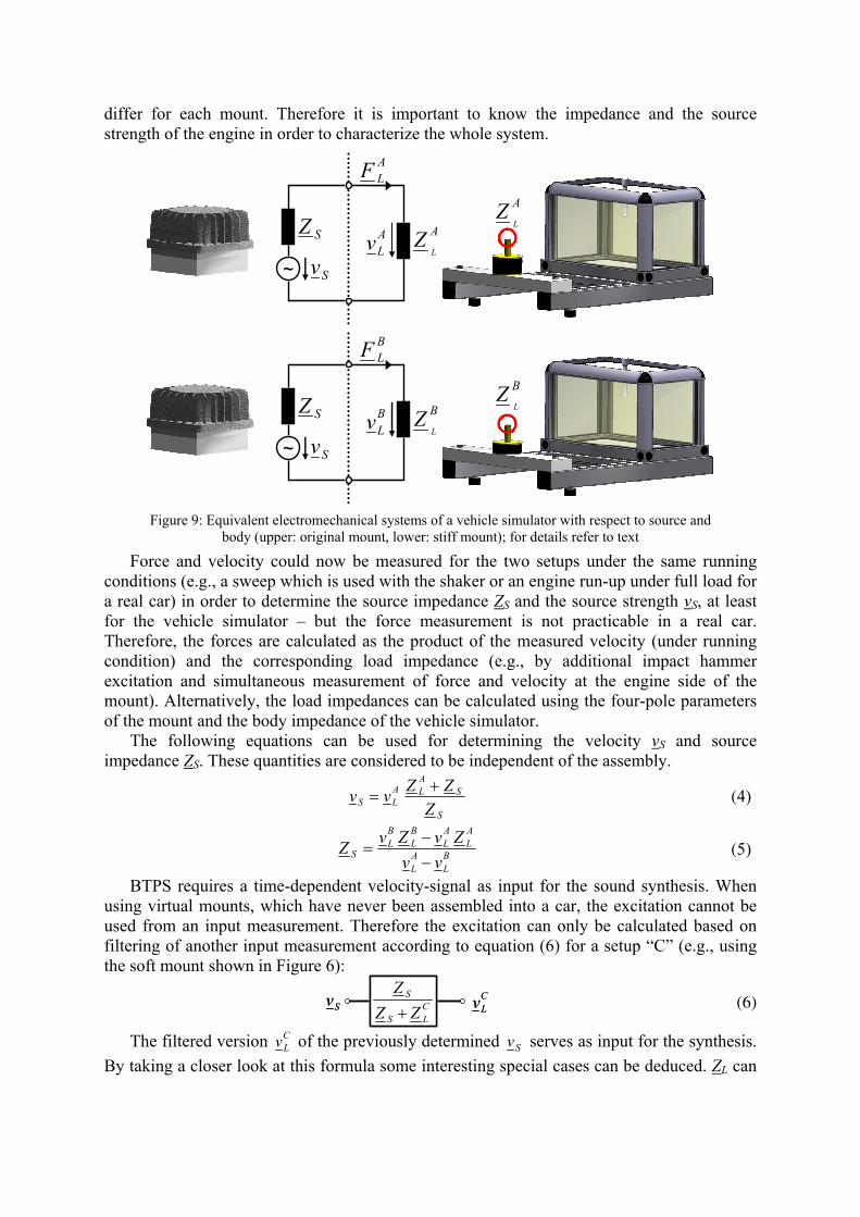
differ for each mount. Therefore it is important to know the impedance and the source strength of the engine in order to characterize the whole system.

~

SZ

SvALv

AL

Z

ALF

~

SZ

SvBLv

BL

Z

BLF

AL

Z

BL

Z

Figure 9: Equivalent electromechanical systems of a vehicle simulator with respect to source and

body (upper: original mount, lower: stiff mount); for details refer to text

Force and velocity could now be measured for the two setups under the same running conditions (e.g., a sweep which is used with the shaker or an engine run-up under full load for a real car) in order to determine the source impedance ZS and the source strength vS, at least for the vehicle simulator – but the force measurement is not practicable in a real car. Therefore, the forces are calculated as the product of the measured velocity (under running condition) and the corresponding load impedance (e.g., by additional impact hammer excitation and simultaneous measurement of force and velocity at the engine side of the mount). Alternatively, the load impedances can be calculated using the four-pole parameters of the mount and the body impedance of the vehicle simulator.

The following equations can be used for determining the velocity vS and source impedance ZS. These quantities are considered to be independent of the assembly.

S

SALA

LS ZZZvv +

= (4)

BL

AL

AL

AL

BL

BL

S vvZvZvZ

−−

= (5)

BTPS requires a time-dependent velocity-signal as input for the sound synthesis. When using virtual mounts, which have never been assembled into a car, the excitation cannot be used from an input measurement. Therefore the excitation can only be calculated based on filtering of another input measurement according to equation (6) for a setup “C” (e.g., using the soft mount shown in Figure 6):

CLS

S

ZZZ+Sv C

LvCLS

S

ZZZ+Sv C

Lv

(6)

The filtered version CLv of the previously determined Sv serves as input for the synthesis.

By taking a closer look at this formula some interesting special cases can be deduced. ZL can

be neglected in equation (6) if it is much smaller than ZS, thus vL is nearly equal to vS: the source can be characterized as a velocity source.

If ZL is much bigger than ZS equation (7) shows that the force FL equals approximately FS: the source can be characterized as a force source.

SCL

CL

ZZZ+SF C

LFS

CL

CL

ZZZ+SF C

LF

(7)

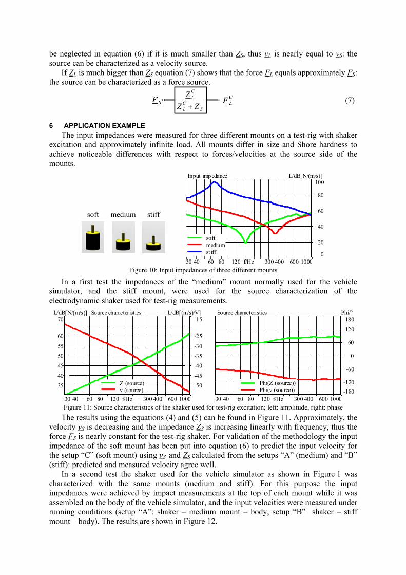
6 APPLICATION EXAMPLE The input impedances were measured for three different mounts on a test-rig with shaker

excitation and approximately infinite load. All mounts differ in size and Shore hardness to achieve noticeable differences with respect to forces/velocities at the source side of the mounts.

softsoft mediummedium stiffstiff

Input impedance L/dB[N/(m/s)]

0

20

40

60

80

100

f/Hz30 40 60 80 120 300 400 600 1000

softmediumst iff

Figure 10: Input impedances of three different mounts

In a first test the impedances of the “medium” mount normally used for the vehicle simulator, and the stiff mount, were used for the source characterization of the electrodynamic shaker used for test-rig measurements.

Source characteristicsL/dB[N/(m/s)] L/dB[(m/s)/V]

-50-45

-40-35-30

-25

-15

3540

455055

60

70

f/Hz30 40 60 80 120 300 400 600 1000

Z (source)v (source)

Source characteristics Phi/°

-180-120

-60

0

60

120

180

f/Hz30 40 60 80 120 300 400 600 1000

Phi(Z (source))Phi(v (source))

Figure 11: Source characteristics of the shaker used for test-rig excitation; left: amplitude, right: phase

The results using the equations (4) and (5) can be found in Figure 11. Approximately, the velocity vS is decreasing and the impedance ZS is increasing linearly with frequency, thus the force FS is nearly constant for the test-rig shaker. For validation of the methodology the input impedance of the soft mount has been put into equation (6) to predict the input velocity for the setup “C” (soft mount) using vS and ZS calculated from the setups “A” (medium) and “B” (stiff): predicted and measured velocity agree well.

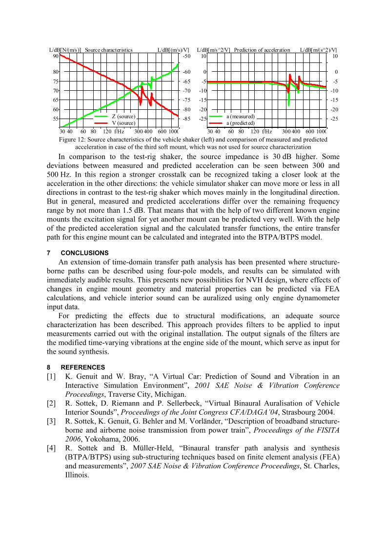
In a second test the shaker used for the vehicle simulator as shown in Figure 1 was characterized with the same mounts (medium and stiff). For this purpose the input impedances were achieved by impact measurements at the top of each mount while it was assembled on the body of the vehicle simulator, and the input velocities were measured under running conditions (setup “A”: shaker – medium mount – body, setup “B” shaker – stiff mount – body). The results are shown in Figure 12.

Source characteristicsL/dB[N/(m/s)] L/dB[(m/s)/V]

-85-80

-75-70-65

-60

-50

5560

657075

80

90

f/Hz30 40 60 80 120 300 400 600 1000

Z (source)V (source)

Prediction of accelerationL/dB[m/s^2/V] L/dB[m/(s^2)/V]

-25-20

-15-10-5

0

10

-25-20

-15-10-5

0

10

f/Hz30 40 60 80 120 300 400 600 1000

a (measured)a (predicted)

Figure 12: Source characteristics of the vehicle shaker (left) and comparison of measured and predicted

acceleration in case of the third soft mount, which was not used for source characterization In comparison to the test-rig shaker, the source impedance is 30 dB higher. Some

deviations between measured and predicted acceleration can be seen between 300 and 500 Hz. In this region a stronger crosstalk can be recognized taking a closer look at the acceleration in the other directions: the vehicle simulator shaker can move more or less in all directions in contrast to the test-rig shaker which moves mainly in the longitudinal direction. But in general, measured and predicted accelerations differ over the remaining frequency range by not more than 1.5 dB. That means that with the help of two different known engine mounts the excitation signal for yet another mount can be predicted very well. With the help of the predicted acceleration signal and the calculated transfer functions, the entire transfer path for this engine mount can be calculated and integrated into the BTPA/BTPS model.

7 CONCLUSIONS An extension of time-domain transfer path analysis has been presented where structure-

borne paths can be described using four-pole models, and results can be simulated with immediately audible results. This presents new possibilities for NVH design, where effects of changes in engine mount geometry and material properties can be predicted via FEA calculations, and vehicle interior sound can be auralized using only engine dynamometer input data.

For predicting the effects due to structural modifications, an adequate source characterization has been described. This approach provides filters to be applied to input measurements carried out with the original installation. The output signals of the filters are the modified time-varying vibrations at the engine side of the mount, which serve as input for the sound synthesis.

8 REFERENCES [1] K. Genuit and W. Bray, “A Virtual Car: Prediction of Sound and Vibration in an

Interactive Simulation Environment”, 2001 SAE Noise & Vibration Conference Proceedings, Traverse City, Michigan.

[2] R. Sottek, D. Riemann and P. Sellerbeck, “Virtual Binaural Auralisation of Vehicle Interior Sounds”, Proceedings of the Joint Congress CFA/DAGA’04, Strasbourg 2004.

[3] R. Sottek, K. Genuit, G. Behler and M. Vorländer, “Description of broadband structure-borne and airborne noise transmission from power train”, Proceedings of the FISITA 2006, Yokohama, 2006.

[4] R. Sottek and B. Müller-Held, “Binaural transfer path analysis and synthesis (BTPA/BTPS) using sub-structuring techniques based on finite element analysis (FEA) and measurements”, 2007 SAE Noise & Vibration Conference Proceedings, St. Charles, Illinois.