CAV2001:sessionB2.005 1

NUMERICAL STUDY OF UNSTEADY CAVITATION ON AHYDROFOIL SECTION USING A BAROTROPIC MODEL

Ciro Pascarella∗ and Vito Salvatore†

CIRA, Italian Aerospace Research CentreCapua, CE, Italy 81043

Abstract

A numerical study on the simulation of cavitation by means of a laminar 2D Navier Stokes flow solver ispresented in this study. In particular, results for cases of cavitating flow around a NACA0015 hydrofoil atdifferent angle of attack are reported. A barotropic relationship is implemented to take in to account theliquid-vapor phase change. The variations both of the flow dynamic response and of the main flow featuresassociated with different values of angles of attack are reported and discussed.

1 Introduction

The difficulty in the numerical modeling of cavitating flows using both an one-fluid (homogeneous) approach(Delannoy and Keuny, 1998, Kubota et al., 1992, Avva and Singhai, 1995, and Chen and Heister, 1994(a))and a two-phase approach (Chen and Heister, 1994(b), De Jong and Sabnis, 1991) is well known.

This paper deals with a numerical method belonging to the first family and, in particular, reports a workon the simulation of unsteady homogeneous cavitating flows in thermal equilibrium conditions.

A cavitating fluid often corresponds to a complicated situation from a numerical point of view; in fact,both incompressible zones (pure phases) and regions where the flow may become highly supersonic (liquid-vapor mixtures) are present in the flow field and need to be resolved. The numerical stiffness of the phe-nomenon is further increased both from the high density ratio between the two phases (for water at 293 Kthe density ratio is equal to O(104) and from the strong shock discontinuity occurring at re-condensation.This singular behaviour is due to the huge variation of speed of sound as the flow goes from a pure phase toa mixture. For instance, in the same hypothesis indicated above, the speed of sound is equal to about 1500m/s for the liquid phase, 400 m/s for vapor phase and 3.2 m/s for a liquid-vapor mixture corresponding toa value of void fraction equal to 0.5 (Jacobsen, 1964).

Moreover, the latter value of minimum speed of sound is calculated in thermal equilibrium conditionsand neglecting both the exchange of mass between the two phases and the surface tension effects. Indeed,the calculation of minimum speed of sound can vary largely depending on the hypothesis that one assumes.For example, using the steam tables (Rivkin, 1988) and assuming cavitation as an isenthalpic transformation(Avva, 1995), the minimum speed of sound at 293 K is approximately equal to 0.004 m/s. In addition, thespeed of sound is a parameter that can be easily defined only when the thermodynamics of phase changeis very fast or very slow (frozen - equilibrium with respect to the characteristic time of the phenomenon(Brennen, 1995). For all the other cases a speed of sound cannot be simply defined.

This paper will not deal with the physical uncertainty in the definition of the correct speed of sound,which is still an open problem. The present research focuses on the capability of the numerical method tocapture the main relevant aspects of cavitating flows. Computations were made on a two-dimensional flowfield around a NACA0015 hydrofoil at different angle of attack, assuming viscous flow.

∗Mechanical Engineer, Member ASME, c.pascarella@cira.it†Aerospace Engineer, v.salvatore@cira.it

CAV2001:sessionB2.005 2

2 Cavitating flow model

All the past main efforts to numerically model cavitating flows can be roughly divided into two classes:interface tracking and continuum methods. In the first case, each phase is treated separately and, typically,there are separate balance equations for each phase. The procedure starts with a tentative surface (atentative interface between two phases) that during the calculation is iteratively updated. The interfacetracking methods have been successfully applied to 2-D flows (Brewe, 1986, Vijayaraghavan and Keith,1990, Deshande and Merkle, 1979, and Chen and Heister, 1994(b)). These methods present two maindisadvantages: they are computationally expensive, due to the double number of balance equations, andthey cannot be easily extended to 3-D flows because of the obvious difficulties involved in tracking complexinterfaces in space. Continuum methods treat the flow as a homogeneous mixture employing a ”void fraction”variable to quantify the intensity of cavitation; this variable is defined as the ratio between the vapor volumeand the whole volume (liquid plus vapor).Continuum methods can be sub-divided into three categories: analyses introducing a vapor source productionterm, analyses including the bubble dynamics and analyses assuming a barotropic state law. The model thatemploys a vapor production equation (Song and He, 1998) resolves, together with the momentum andcontinuity equations for the mixture, the following phasic continuity equation when p < pV :

Dρ

Dt= S = CV (p− pV ) (1)

This approach imposes the choice of the empirical coefficient CV that, unfortunately, depends on severalparameters such as properties of the fluid, body geometry and other flow conditions. Furthermore, being thenumerical solutions very sensitive to the choice of CV , the use of this method seems to be confined only toacademic purposes. Kubota et al (1992) proposed one of the earliest continuum methods. In his approachhe treats the cavitating flow as a uniform mixture of liquid and very little bubbles. The mathematicalformulation of the problem is very rigorous: the growth and the collapse of bubble clusters is taken intoaccount by the introduction of a modified Raleigh’s equation. Also this method has free, user-suppliedconstants, that are the initial radii and initial number density of the bubbles. Another limitation of themethod proposed by Kubota et al. (1992) is represented by the severe stability problems encountered atlow void fractions, which makes this approach not easily applicable to any cavitating flow. Analyses in thethird category assume the existence of an effective barotropic relation for the homogeneous mixture. Thebarotropic relation ρ = ρ(p) assumes that the fluid pressure is a function of fluid density only. This impliesthat all the effects caused by bubble content are disregarded except for the compressibility and that thebubbly mixture can be regarded as a single-phase compressible fluid. Usually, the methods employing abarotropic state law, such as that proposed here, assume a continuous variation of density between liquidand vapor values in a range of pressures centered at the vapor pressure. Such a variation can be representedby a sinusoidal curve (Delannoy and Keuny, 1998), by a polynomial curve (Song and He, 1998), etc. Inall cases, the maximum slope of the curve occurs at the vapor pressure. For the present study a simplesinusoidal law has been chosen.

The following relation represents the barotropic variation in the two-phase zone:

ρ = ρV +1

a2min

2

π(p − pV )sin(

p− pVpL − pV

π

2) (2)

where amin , the minimum speed of sound, is the parameter that determines the maximum slope of thebarotropic curve and

ρV =ρL + ρG

2(3)

pL = pV + (ρL − ρV )a2min

π

2(4)

pG = 2pV − pL (5)

The density derivative with respect to pressure is

CAV2001:sessionB2.005 3

1

a2=dρ

dp=

1

a2min

cos(p− pVpL − pV

π

2) (6)

And so one finds that the speed of sound goes to infinity for p = pG and for p = pL (incompressibleregions) and is equal to amin for p = pV .

For this approach, it is necessary to specify three constants: the minimum speed of sound, the liquiddensity and the vapor density. For the last two properties one can choose the density values corresponding tothe equilibrium conditions (for fixed temperature). A reasonable value of amin could be assumed within therange limited by the values obtained following either the so called dynamic approach of Jakobsen (1964) orthe isenthalpic transformation approach proposed by Avva (1995). These two approaches give very differentvalues of minimum speed of sound. Following the dynamic approach, the mass and heat transfer betweenthe two phases is neglected. The thermodynamic transformation is assumed to be isentropic for each phase.

In these hypotheses the speed of sound in the homogeneous flow is

1

a2=

1

a2V

[α2 + α(1− α)ρLρV

] +1

a2L

[(1− α)2 + α(1− α)ρVρL

] (7)

where α is the void fraction, defined as

α =1− ρ/ρL

1− ρV /ρL(8)

In the isenthalpic transformation, the two phases are assumed in thermal equilibrium. Using the thermo-dynamic tables (RivKin, 1988) it is possible, if a value of enthalpy h is fixed, to establish a correspondencebetween pressure and density for the homogeneous mixture, therefore defining a barotropic relationship fromwhich the speed of sound can be easily derived.

3 Numerical approach

In the homogeneous approach and in the hypothesis of thermodynamic equilibrium the governing equationsto solve are the Navier Stokes equations written in the unsteady, compressible form for one phase withoutthe energy conservation equation; the barotropic state law completes the set of equations. The model maybe written as two vectorial partial differential equations and one algebraic equation of state:

∂ρ

∂t+∇ · (ρV) = 0 (9)

∂ρV

∂t+∇ · (ρVV) = −∇p +∇ · (µ∇V) (10)

ρ = ρ(p) (11)

where ρ and µ are, respectively, the density and the viscosity of the mixture. The barotropic law of state,eq. (2), defines the value of the density; a simple and stable way to calculate µ is the following (Kubota etal., 1992):

µ = µG · α+ µL(1− α) (12)

where ρG and ρL are the vapor viscosity and the liquid viscosity respectively, and α is the void frac-tion. The choice of the numerical method to approach cavitation is very critical. In fact a cavitating flowpresents huge gradients at the liquid-vapor interface. Furthermore, the flow field goes from incompressiblein the one-phase regions to highly supersonic where a liquid-vapor mixture is present. Thus, the mainrequirements for the flow solver are the capability to work well in a wide Mach number spectrum, fromzero to Mach >> 1, and the shock-capturing or interface-capturing property in order to solve correctly theliquid-vapor surface discontinuity. The most suitable methodology to solve the governing equations seemsto be a pressure-based method with a finite volume discretization written in conservative form, based onthe SIMPLE (Semi Implicit Method for Pressure Linked Equations) algorithm (Patankar, 1980), with Karki

CAV2001:sessionB2.005 4

(1986) compressibility correction. The code developed in the present work, named ALL2D, can be appliedto both plane and axi-symmetric configurations; under steady or unsteady conditions, and can be used tosimulate both inviscid and viscous laminar flows. In the developed code a non oscillatory TVD 2nd / 1st

order scheme, derived from SMART (Gaskel, and Lau, 1988), is adopted.ALL2D works with a body-fitted grid; the governing equations (9)-(10) have been reported here only in

a Cartesian coordinate system for simplicity; in any case, applying the tensor rules, the system of equations(9)-(10) can be transformed in an equivalent system written in a curvilinear reference frame. The actualform of the governing is more and can be found in Kadja and Leschziner (1987). As in all the methodsderived from the SIMPLE algorithm, also in ALL2D it is necessary to execute the so-called under-relaxationat the end of each iteration to promote stability; the value of the general variable φ at location L may beexpressed by:

φ = αφφoldL + (1− αφ)φnewL (13)

where α is a value between zero and one. Particular attention must be paid when the flow is cavitating;in this case, to avoid abrupt oscillations of density, the under-relaxation of pressure must be limited byimposing values to the pressure correction always less than (pL − pV ). A way to achieve this is to introducea varying under-relaxation factor which depends on the pressure correction itself as follows:

αP =pL − pV∆Pmax

1

χ(14)

where ∆Pmax is the maximum value of pressure correction and χ is an arbitrary number greater thanone.

4 Validation

The numerical method has been validated using the experimental data available from Rouse and McNown(1948), consisting in pressure measurements on the surface of some head forms at zero angle of yaw inwater under steady s tate conditions. Although these experiments are very old the data are quite reliable. Ingeneral, it is very hard to find reliable experimental data on cavitating flows. Among the several tests reportedin Rouse and McNown (1948) two different head form shapes have been chosen. Both head forms belongto the so-called ”Rounded Series”; in particular, they are called ”2in.-Caliber Ogival” and ”Hemispherical”.The comparison between numerical and experimental data has been made for each geometry at two differentflow conditions corresponding to incipient cavitation and fully developed cavitation, see Table (1). Followingthe terminology adopted in Rouse and McNown (1948) a cavitation index K has been defined as:

K =p∞ − pLp0 − p∞

(15)

The simulations have been performed neglecting the viscous effects (Euler approximation) and assuminga minimum speed of sound of 0.12 m/s.

The calculations have been carried out assuming a temperature of 320 K; the corresponding density ratiois equal to 13305 (989/0.072) and the vapor pressure is equal to 10530 Pa. Both the very high density ratioand the very low speed of sound represent quite severe conditions: in most of the works in the literature onnumerical modeling of cavitation using a barotropic law of state, a maximum value of density ratio of 1000and a minimum sp eed of sound of 0.5-1 m/s is reported in Delannoy and Keuny (1998) and Hoeijmakers etal. (1998), for example. For all simulations the total pressure at inlet and the static pressure at outlet havebeen imposed as boundary conditions.

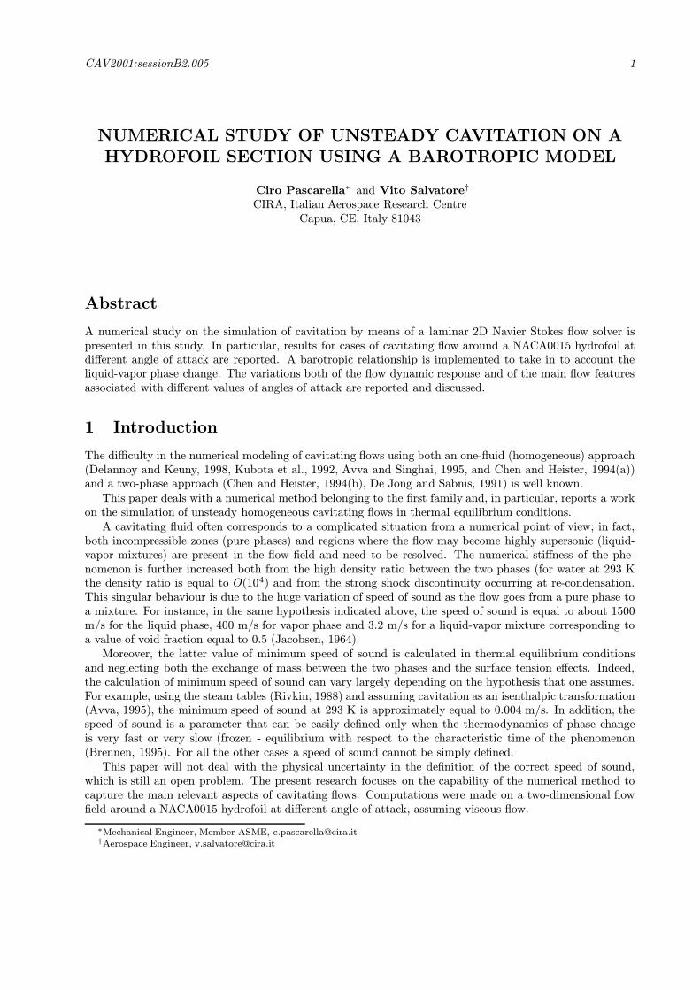
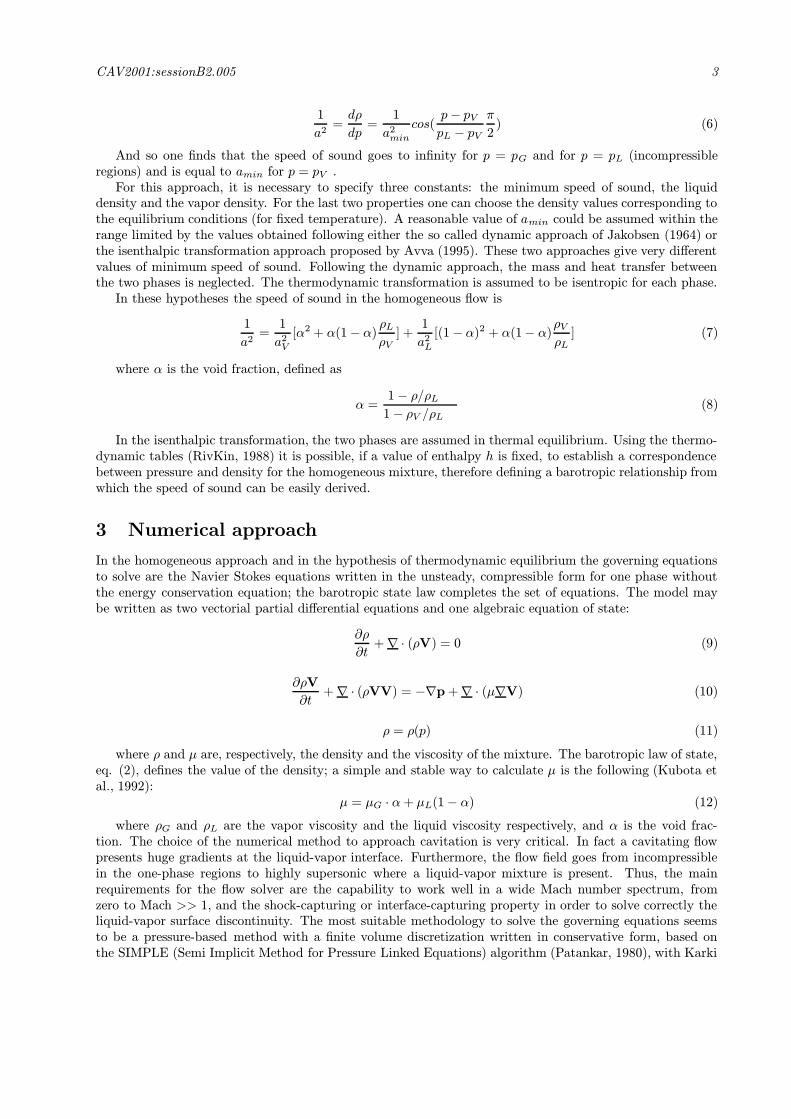
The comparison between calculated and measured Cp distributions along the surface of the ogival headform is shown in Figure (1),a, for the case of incipient cavitation, as shown by the small zone where the Cpremains almost constant. A good agreement between computed and experimental values is attained. Thisagreement is still good for the fully developed cavitation case, as shown in Figure (1),b, : the length ofthe vapor bubble has been captured rather well. The discrepancy in the re-condensation zone, where thecomputation shows a shock, is probably due to thermal non-equilibrium effects. Figure (2),a, shows the

CAV2001:sessionB2.005 5

Test Ogival Headform Hemispherical Headform

1 K=0.3 Incipient Cavitation K=0.7 Incipient Cavitation2 K=0.2 Developed Cavitation K=0.2 Developed Cavitation

Table 1: Validation Test Run Matrix

-0.8

-0.6

-0.4

-0.2

0

0.2

0.4

0.6

0.8

1

1.2

0 1 2 3 4 5 6

CP

S

computation experimental data

-0.8

-0.6

-0.4

-0.2

0

0.2

0.4

0.6

0.8

1

1.2

0 1 2 3 4 5 6

CP

S

computation experimental data

Figure 1: Ogival Headform. a: Incipient Cavitation, K=0.3. b: Developed Cavitation, K=0.2

Cp distribution on the hemispherical head form corresponding to the onset of cavitation; the comparison ofnumerical and experimental values is again quite satisfactory.

The most severe case is represented the fully developed cavitation on the hemispherical head form. Alsofor this case, agreement is excellent up to the end of the cavity where some discrepancy can be noted atre-condensation, Figure (2),b, More details can be found in Pascarella et al. (2000).

5 Results

The goal of this work is to investigate the dynamic response of the cavitating flow field around a NACA0015hydrofoil at different angles of attack. Water at temperature of 323 K, that corresponds to an enthalpy equal

-0.8

-0.6

-0.4

-0.2

0

0.2

0.4

0.6

0.8

1

1.2

0 1 2 3 4 5 6

CP

S

computation experimental data

-0.6

-0.4

-0.2

0

0.2

0.4

0.6

0.8

1

1.2

1.4

0 1 2 3 4 5 6

CP

S

computationexperimental data

Figure 2: Hemispherical Headform. a: Incipient Cavitation, K=0.7. b: Developed Cavitation, K=0.2

CAV2001:sessionB2.005 6

n α σ amin Vinlet P∞1 4o 1.0 3.0 m/s 3.0 m/s 23789 Pa2 8o 1.0 3.0 m/s 3.0 m/s 23789 Pa

Table 2: Computation matrix

to 200 kJ/kg, has been chosen as working fluid.The value of the minimum speed of sound of the sinusoidal barotropic model has been set equal to 3.0

m/s (see Pascarella et al., 2001), in the range defined by the isenthalpic model (Avva, 1995) and the dynamicapproach (Jacobsen, 1964), that, under these conditions, give the following values, respectively:

Isoenthalpic model: amin = 0.17 m/sDynamic approach: amin = 8.16 m/s

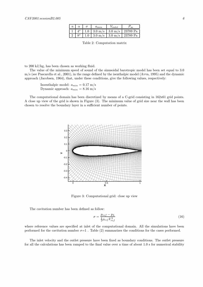
The computational domain has been discretized by means of a C-grid consisting in 162x61 grid points.A close up view of the grid is shown in Figure (3). The minimum value of grid size near the wall has beenchosen to resolve the boundary layer in a sufficient number of points.

X

Y

0 0.5 1

-0.4

-0.3

-0.2

-0.1

0

0.1

0.2

0.3

Figure 3: Computational grid: close up view

The cavitation number has been defined as follow:

σ =pref − pL12ρrefV

2ref

(16)

where reference values are specified at inlet of the computational domain. All the simulations have beenperformed for the cavitation number σ=1 . Table (2) summarizes the conditions for the cases performed.

The inlet velocity and the outlet pressure have been fixed as boundary conditions. The outlet pressurefor all the calculations has been ramped to the final value over a time of about 1.0 s for numerical stability

CAV2001:sessionB2.005 7

Thermodynamic Properties

Temperature T 323 KLiquid Density ρL 988 kg/m3

Vapor Density ρG 0.083 kg/m3

Vapor Pressure pV 12352 PaLiquid Sound Speed aL 1542 m/sVapor Sound Speed aG 443 m/s

Table 3: Thermodynamic Properties of Water @ 323 K

Time [s]

Poi

nts

0 0.2 0.4 0.6 0.8 1 1.2 1.4 1.6 1.8 2 2.2 2.4 2.6 2.8 3 3.2 3.4 3.6 3.8 4 4.2 4.4 4.6 4.8 50

100

200

300

400

Time [s]

Pre

ssur

e[P

a]

0.4 0.6 0.8 1 1.2 1.4 1.6 1.8 2 2.2 2.4 2.6 2.8 3 3.2 3.4 3.6 3.8 4 4.2 4.4 4.6 4.8 527000

27250

27500

27750

28000

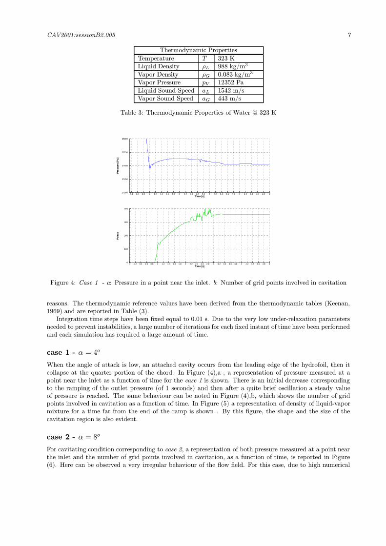
Figure 4: Case 1 - a: Pressure in a point near the inlet. b: Number of grid points involved in cavitation

reasons. The thermodynamic reference values have been derived from the thermodynamic tables (Keenan,1969) and are reported in Table (3).

Integration time steps have been fixed equal to 0.01 s. Due to the very low under-relaxation parametersneeded to prevent instabilities, a large number of iterations for each fixed instant of time have been performedand each simulation has required a large amount of time.

case 1 - α = 4o

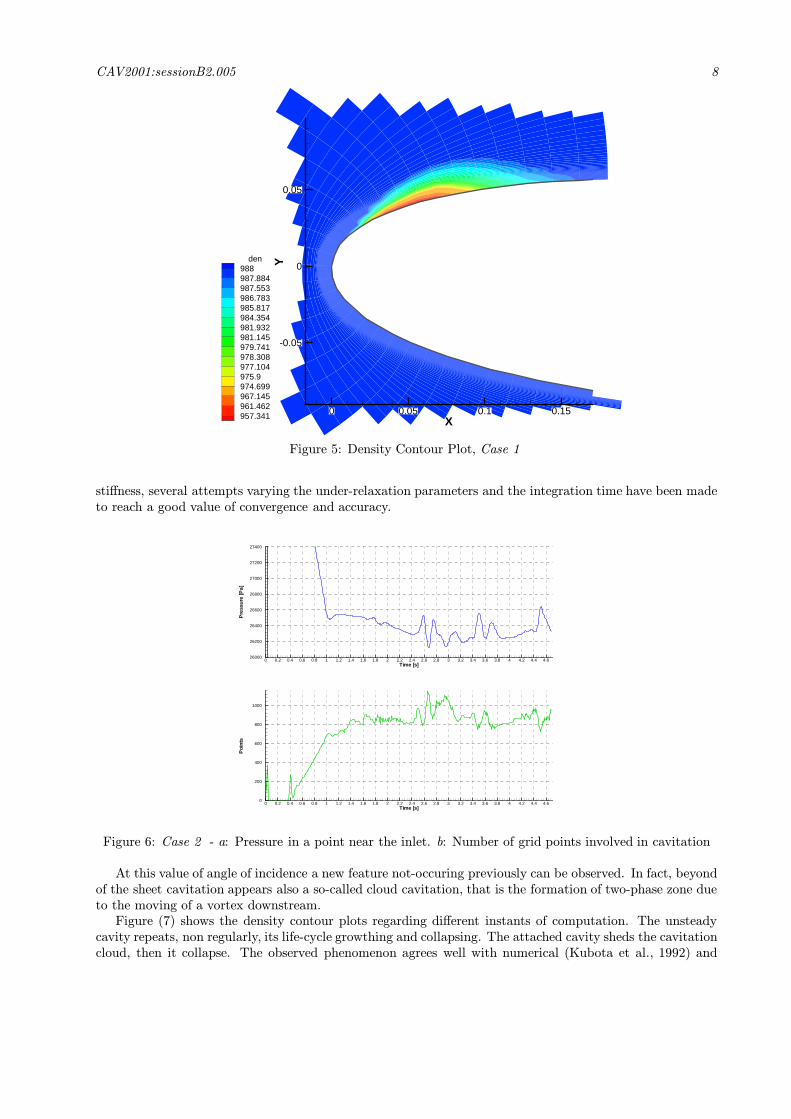
When the angle of attack is low, an attached cavity occurs from the leading edge of the hydrofoil, then itcollapse at the quarter portion of the chord. In Figure (4),a , a representation of pressure measured at apoint near the inlet as a function of time for the case 1 is shown. There is an initial decrease correspondingto the ramping of the outlet pressure (of 1 seconds) and then after a quite brief oscillation a steady valueof pressure is reached. The same behaviour can be noted in Figure (4),b, which shows the number of gridpoints involved in cavitation as a function of time. In Figure (5) a representation of density of liquid-vapormixture for a time far from the end of the ramp is shown . By this figure, the shape and the size of thecavitation region is also evident.

case 2 - α = 8o

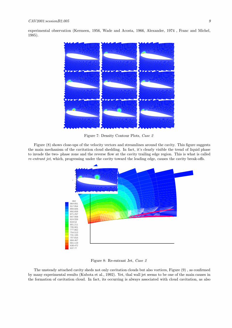
For cavitating condition corresponding to case 2, a representation of both pressure measured at a point nearthe inlet and the number of grid points involved in cavitation, as a function of time, is reported in Figure(6). Here can be observed a very irregular behaviour of the flow field. For this case, due to high numerical

CAV2001:sessionB2.005 8

X

Y

0 0.05 0.1 0.15

-0.05

0

0.05

den988987.884987.553986.783985.817984.354981.932981.145979.741978.308977.104975.9974.699967.145961.462957.341

Figure 5: Density Contour Plot, Case 1

stiffness, several attempts varying the under-relaxation parameters and the integration time have been madeto reach a good value of convergence and accuracy.

Time [s]

Poi

nts

0 0.2 0.4 0.6 0.8 1 1.2 1.4 1.6 1.8 2 2.2 2.4 2.6 2.8 3 3.2 3.4 3.6 3.8 4 4.2 4.4 4.60

200

400

600

800

1000

Time [s]

Pre

ssur

e[P

a]

0 0.2 0.4 0.6 0.8 1 1.2 1.4 1.6 1.8 2 2.2 2.4 2.6 2.8 3 3.2 3.4 3.6 3.8 4 4.2 4.4 4.626000

26200

26400

26600

26800

27000

27200

27400

Figure 6: Case 2 - a: Pressure in a point near the inlet. b: Number of grid points involved in cavitation

At this value of angle of incidence a new feature not-occuring previously can be observed. In fact, beyondof the sheet cavitation appears also a so-called cloud cavitation, that is the formation of two-phase zone dueto the moving of a vortex downstream.

Figure (7) shows the density contour plots regarding different instants of computation. The unsteadycavity repeats, non regularly, its life-cycle growthing and collapsing. The attached cavity sheds the cavitationcloud, then it collapse. The observed phenomenon agrees well with numerical (Kubota et al., 1992) and

CAV2001:sessionB2.005 9

experimental observation (Kermeen, 1956, Wade and Acosta, 1966, Alexander, 1974 , Franc and Michel,1985).

Figure 7: Density Contour Plots, Case 2

Figure (8) shows close-ups of the velocity vectors and streamlines around the cavity. This figure suggeststhe main mechanism of the cavitation cloud shedding. In fact, it’s clearly visible the trend of liquid phaseto invade the two- phase zone and the reverse flow at the cavity trailing edge region. This is what is calledre-entrant jet, which, progressing under the cavity toward the leading edge, causes the cavity break-offs.

den964.651917.954894.605892.659871.257847.908824.559819.52801.211795.901777.862754.513731.165707.816684.467661.119638.472637.77

X

Y

0 0.25 0.5 0.75

-0.2

-0.1

0

0.1

0.2

Figure 8: Re-entrant Jet, Case 2

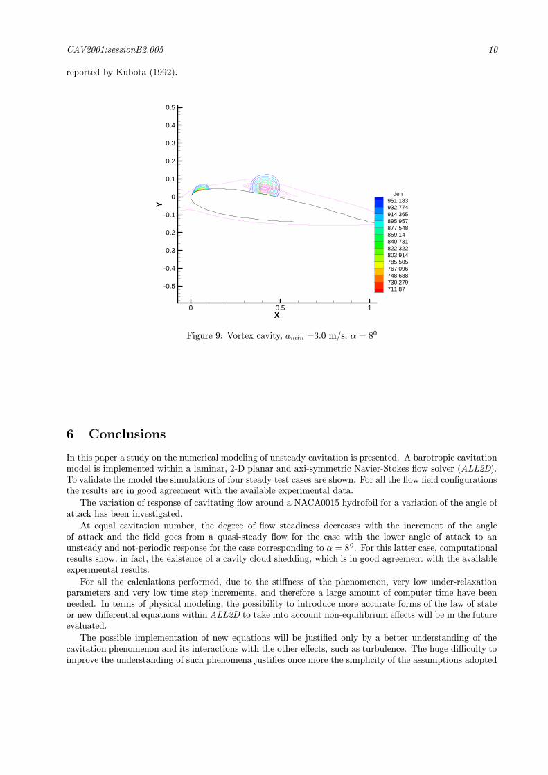
The unsteady attached cavity sheds not only cavitation clouds but also vortices, Figure (9) , as confirmedby many experimental results (Kubota et al., 1992). Yet, thal wall jet seems to be one of the main causes inthe formation of cavitation cloud. In fact, its occurring is always associated with cloud cavitation, as also

CAV2001:sessionB2.005 10

reported by Kubota (1992).

X

Y

0 0.5 1

-0.5

-0.4

-0.3

-0.2

-0.1

0

0.1

0.2

0.3

0.4

0.5

den951.183932.774914.365895.957877.548859.14840.731822.322803.914785.505767.096748.688730.279711.87

Figure 9: Vortex cavity, amin =3.0 m/s, α = 80

6 Conclusions

In this paper a study on the numerical modeling of unsteady cavitation is presented. A barotropic cavitationmodel is implemented within a laminar, 2-D planar and axi-symmetric Navier-Stokes flow solver (ALL2D).To validate the model the simulations of four steady test cases are shown. For all the flow field configurationsthe results are in good agreement with the available experimental data.

The variation of response of cavitating flow around a NACA0015 hydrofoil for a variation of the angle ofattack has been investigated.

At equal cavitation number, the degree of flow steadiness decreases with the increment of the angleof attack and the field goes from a quasi-steady flow for the case with the lower angle of attack to anunsteady and not-periodic response for the case corresponding to α = 80. For this latter case, computationalresults show, in fact, the existence of a cavity cloud shedding, which is in good agreement with the availableexperimental results.

For all the calculations performed, due to the stiffness of the phenomenon, very low under-relaxationparameters and very low time step increments, and therefore a large amount of computer time have beenneeded. In terms of physical modeling, the possibility to introduce more accurate forms of the law of stateor new differential equations within ALL2D to take into account non-equilibrium effects will be in the futureevaluated.

The possible implementation of new equations will be justified only by a better understanding of thecavitation phenomenon and its interactions with the other effects, such as turbulence. The huge difficulty toimprove the understanding of such phenomena justifies once more the simplicity of the assumptions adopted

CAV2001:sessionB2.005 11

in this work for the state law approximation. Despite this approximation, the results obtained at the presentstage of this project are surprisingly encouraging.

Acknowledgements

The authors would like to thank Dr. L. d’Agostino of the University of PISA for the helpful discussions oncavitation modeling.

The investigations were carried out at CIRA (Italian Center for Aerospace Research) in the frameworkof CFD applied to propulsive system.

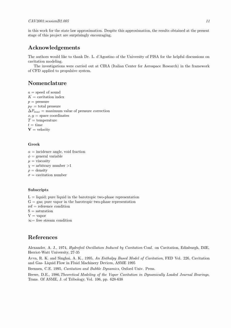
Nomenclature

a = speed of soundK = cavitation indexp = pressurepT = total pressure∆Pmax = maximum value of pressure correctionx, y = space coordinatesT = temperaturet = timeV = velocity

Greek

α = incidence angle, void fractionφ = general variableµ = viscosityχ = arbitrary number >1ρ = densityσ = cavitation number

Subscripts

L = liquid; pure liquid in the barotropic two-phase representationG = gas; pure vapor in the barotropic two-phase representationref = reference conditionS = saturationV = vapor∞= free stream condition

References

Alexander, A. J., 1974, Hydrofoil Oscillation Induced by Cavitation Conf. on Cavitation, Edinburgh, IME,Herriot-Watt University, 27-35

Avva, R. K. and Singhai, A. K., 1995, An Enthalpy Based Model of Cavitation, FED Vol. 226, Cavitationand Gas- Liquid Flow in Fluid Machinery Devices, ASME 1995

Brennen, C.E. 1995, Cavitation and Bubble Dynamics, Oxford Univ. Press.

Brewe, D.E., 1986,Theoretical Modeling of the Vapor Cavitation in Dynamically Loaded Journal Bearings,Trans. Of ASME, J. of Tribology, Vol. 106, pp. 628-638

CAV2001:sessionB2.005 12

Chen , Y. and Heister, D. S., 1994(a), Two Phase Modeling of Cavitated Flows, FED-Vol 190, ASMECavitation and gas-liquid Flow in Fluid-Machinery and Devices Forum

Chen , Y. and Heister, D. S., 1994(b), A Numerical Treatment for Attached Cavitation, J. Of Fluid Eng.,Sep tember, Vol.116

De Jong, F. J. and Sabnis, J. F. ,1991, Simulation of Cryogenic Liquid Flows with Vapor Bubbles, AIAA-91-2257

Delannoy, Y. and Kueny, J. L., 1998 Two-Phase Approach in Unsteady Cavitation Modeling, FED Vol. 98,ASME Cavitation and Multiphase Flow Forum, Grenoble, France

Deshande, M. and Merkle, C., 1979, Cavity Flow Predictions Based on Euler Equation, Trans. Of ASME,J. Fluid Eng., Vol. 116, pp. 36-44

Franc, J. P. and Michel, J.M., 1985 Attached Cavitation and Boundary Layer: Experimental Investigationand Numerical Treatment, J. Fluid Mech., 154, 63-90

Gaskell, P., H. and Lau, K. C. , 1988, Curvature Compensate Convective Transport: SMART, a New Bounde-ness Preserving Transport Algorithm, International Journal for Numerical Methods in Fluids, 8, pp. 617-641

Hoeijmakers, H. W. M., Janssens, M. E. and Kwon, W., 1998, Numerical Simulation of Sheet Cavitation,3nd International Symposium On Cavitation, Grenoble, France

Jakobsen, J., K., 1964, On The Mechanism of Head Breakdown in Cavitating Inducer, J. Of Basic Eng.,Trans. ASME, June 1 964, pp. 291-305

Kadja, M. and Leschziner, M., A., 1987 The Team-Cog Computer Code, UMIST, Draft1

Karki, K.C., 1986, Ph.D. Thesis, Minnesota State University.

Kermeen, R.W., 1956,Water Tunnel Test of NACA0012 and Walchner Profile 7 Hydrofoil in Non-Cavitatingand Cavitating flows. Hydrodynamic Laboratory, California institute of Technology, Pasadena, California,Rep. No. 47-5

Kubota, A., Kato, H. and Yamaguchi, H., 1992, A New Modeling of Cavitating Flows; a Numerical Study ofUnsteady Cavitation on a Hydrofoil Section, Journal of Fluid Mechanics, Vol. 240, pp 59-96

Pascarella, C., Ciucci, A., Salvatore V. and d’Agostino L., A Numerical Tool for the Investigation of Cavitat-ing Flows in Turbopump Inducers, 36th AIAA/ASME/SAE/ASEE Joint Propulsion Conference and Exhibit,July 17-19 2000, Huntsville, AL, USA

Pascarella, C., Ciucci, A. and Salvatore V., Numerical Study on the Effects of Speed of Sound Variation onUnsteady Cavitating Flows , Submitted to Trans. Of ASME, J. Fluid Eng.

Patankar, S. V., 1980, Numerical Heat Transfer and Fluid Flow, Hemisphere Publishing Corporation.

Rivkin, S.L., 1988, Thermodynamic Properties of Gases, Hemisphere Publishing Corporation.

Rouse, H. and McNown, J., S., 1948, Cavitation and Pressure Distribution: Head Form at Zero Angle ofYaw, State University of IOWA, Eng. Bull.,N.32

Song, C. and He, G., 1998, Numerical Simulation of Cavitating Flow by Single-Phase Flow Approach, 3nd

International Symposium On Cavitation, Grenoble, France

Wade, R. B. and Acosta, A. J. , 1966 Experimental Observation on the Flow Past a Plano-Convex Hydrofoil.Trans. ASME I: J. Fluids Engng 88, 273-283

Vijayaraghavan, D. and Keith, T.,G., 1990, An Efficient, Robust, and Time Accurate Numerical SchemeApplied to a Cavitation Algorithm, Trans. Of ASME, J. Of Tribology, Vol 112, pp. 44-51