UPTEC F 20062

Examensarbete 30 hpDecember 2020

Numerical solutions to high frequency approximations of the scalar wave equation

Carl Sundström

Teknisk- naturvetenskaplig fakultet UTH-enheten Besöksadress: Ångströmlaboratoriet Lägerhyddsvägen 1 Hus 4, Plan 0 Postadress: Box 536 751 21 Uppsala Telefon: 018 – 471 30 03 Telefax: 018 – 471 30 00 Hemsida: http://www.teknat.uu.se/student

Abstract

Numerical solutions to high frequency approximationsof the scalar wave equation

Carl Sundström

Throughout many fields of science and engineering, the need for describing waveequations is crucial. Solving the wave equation for high-frequency waves istime-consuming, requires a fine mesh size and memory usage. The main goal wasimplementing and comparing different solution methods for high-frequency waves.Four different methods have been implemented and compared in terms of runtimeand discretization error. From my results, the method which performs the best is thefast sweeping method. For the fast marching method, the time-complexity of thenumerical solver was higher than expected which indicates an error in myimplementation.

ISSN: 1401-5757, UPTEC F 20062Examinator: Tomas NybergÄmnesgranskare: Maya NeytchevaHandledare: Ivar Bratberg

1 Popularvetenskaplig sammanfattning

En viktig del inom naturvetenskap och ingenjorskonst ar att stalla upp modeller som amnar attbeskriva ett fenomen. Nar till exempel en bro byggs upprattas teoretiska modeller om maxlast forbron som baseras pa fysik och matematik. Experimentell matdata fran liknande broar anvandsocksa for att faststalla modellens tillforlitlighet. For att skapa sig en noggran uppfattning utifranteorin kravs ofta en dator. Teoretiska modeller, empirisk data samt datorsimulering ar tre viktigapelare for att beskriva ett system. Dessa anvands i samspel for att forutse ett systems beteendeMed datorer kan vi idag losa komplexa system som for bara nagra decennier sedan hade varitomojligt. Datorsimuleringar ar, utover ett verktyg for att losa svara teoretiska problem, aven valdigtkostnadseffektivt jamfort med att bygga experimentella anlaggningar. Ett omrade som ar av stortintresse ar att beskriva vagrorelse och vibrationer. Detta da det kan anvandas till exempel for attbeskriva ljus (elektromagnetiska vagor), havsvagor och ljudutbredning. Ett problem som uppstar narman beskriver snabbt svangande vagor ar brist pa datorminne samt lang kortid. For att motverkadetta finns modeller for hogfrekventvagutbredning som ar mer latthanterlig for en dator att losa.Malet med detta arbete har varit att jamfora olika losningsmetoder for hogfrekventvagutbredning.Fyra olika numeriska metoder har jamforts for att se for- och nackdelar. Metoderna har jamfortsmed avseende pa kortid samt diskretiseringsfel. Den metod som presterat bast ar ’the fast sweepingmethod’ som har kort kortid och aven lagt diskretiseringsfel. Det finns aven flera utvecklingsomradenfor framtida arbeten, dar ett av dem ar att utoka metodernas noggrannhetsordning.

3

Acknowledgement

I want thank my supervisors Ivar Bratberg and Jostein Natvig for guiding me throughout this thesis.

I also want to show my appreciation to Maya Neytcheva for being my subject reviewer who helpedme when needed.

4

Contents

1 Popularvetenskaplig sammanfattning 3

2 Introduction 6

3 Background 7

4 Numerical methods 94.1 Domain discretization . . . . . . . . . . . . . . . . . . . . . . . . . . . . . . . . . . . . 9

4.1.1 High resolution flux evaluation . . . . . . . . . . . . . . . . . . . . . . . . . . . 104.2 Numerical solution methods . . . . . . . . . . . . . . . . . . . . . . . . . . . . . . . . . 104.3 Gauss-Seidel iteration . . . . . . . . . . . . . . . . . . . . . . . . . . . . . . . . . . . . 10

4.3.1 Stopping criteria . . . . . . . . . . . . . . . . . . . . . . . . . . . . . . . . . . . 104.4 Eikonal equation . . . . . . . . . . . . . . . . . . . . . . . . . . . . . . . . . . . . . . . 10

4.4.1 Fast sweeping method . . . . . . . . . . . . . . . . . . . . . . . . . . . . . . . . 114.4.2 Fast marching method . . . . . . . . . . . . . . . . . . . . . . . . . . . . . . . . 11

4.5 Transport equation for the amplitude . . . . . . . . . . . . . . . . . . . . . . . . . . . . 124.5.1 Fast sweeping method . . . . . . . . . . . . . . . . . . . . . . . . . . . . . . . . 124.5.2 Time-stepping method . . . . . . . . . . . . . . . . . . . . . . . . . . . . . . . . 13

5 Computer specifications and implementation 13

6 Numerical results 136.1 Input data . . . . . . . . . . . . . . . . . . . . . . . . . . . . . . . . . . . . . . . . . . . 146.2 Performance . . . . . . . . . . . . . . . . . . . . . . . . . . . . . . . . . . . . . . . . . . 15

6.2.1 Eikonal equation . . . . . . . . . . . . . . . . . . . . . . . . . . . . . . . . . . . 166.2.2 Amplitude transport equation . . . . . . . . . . . . . . . . . . . . . . . . . . . . 16

6.3 Convergence . . . . . . . . . . . . . . . . . . . . . . . . . . . . . . . . . . . . . . . . . . 176.3.1 Eikonal equation . . . . . . . . . . . . . . . . . . . . . . . . . . . . . . . . . . . 186.3.2 Amplitude transport equation . . . . . . . . . . . . . . . . . . . . . . . . . . . . 19

6.4 Eikonal equation . . . . . . . . . . . . . . . . . . . . . . . . . . . . . . . . . . . . . . . 216.4.1 Amplitude transport equation . . . . . . . . . . . . . . . . . . . . . . . . . . . . 22

6.5 Displacement approximation . . . . . . . . . . . . . . . . . . . . . . . . . . . . . . . . . 23

7 Discussion 247.1 Eikonal equation . . . . . . . . . . . . . . . . . . . . . . . . . . . . . . . . . . . . . . . 24

7.1.1 Runtime . . . . . . . . . . . . . . . . . . . . . . . . . . . . . . . . . . . . . . . . 247.1.2 Convergence . . . . . . . . . . . . . . . . . . . . . . . . . . . . . . . . . . . . . 25

7.2 Amplitude transport equation . . . . . . . . . . . . . . . . . . . . . . . . . . . . . . . . 257.2.1 Run time . . . . . . . . . . . . . . . . . . . . . . . . . . . . . . . . . . . . . . . 267.2.2 Convergence . . . . . . . . . . . . . . . . . . . . . . . . . . . . . . . . . . . . . 26

8 Conclusion and future work 27

5

2 Introduction

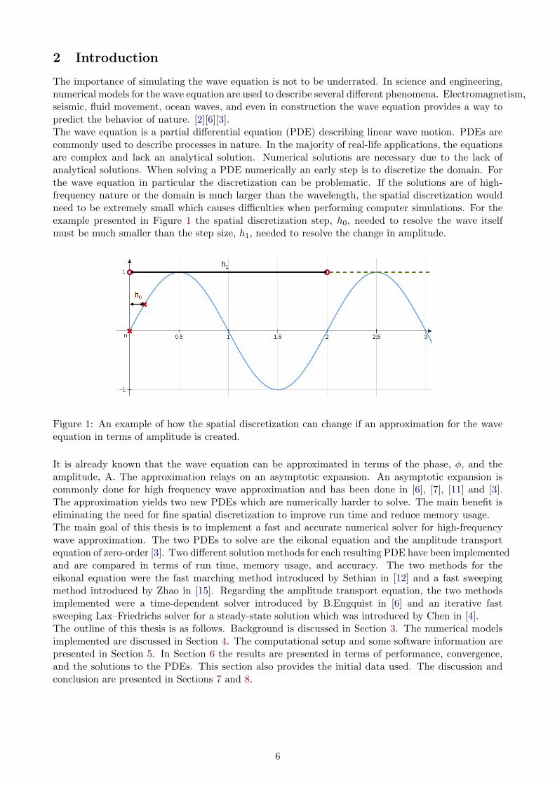
The importance of simulating the wave equation is not to be underrated. In science and engineering,numerical models for the wave equation are used to describe several different phenomena. Electromagnetism,seismic, fluid movement, ocean waves, and even in construction the wave equation provides a way topredict the behavior of nature. [2][6][3].The wave equation is a partial differential equation (PDE) describing linear wave motion. PDEs arecommonly used to describe processes in nature. In the majority of real-life applications, the equationsare complex and lack an analytical solution. Numerical solutions are necessary due to the lack ofanalytical solutions. When solving a PDE numerically an early step is to discretize the domain. Forthe wave equation in particular the discretization can be problematic. If the solutions are of high-frequency nature or the domain is much larger than the wavelength, the spatial discretization wouldneed to be extremely small which causes difficulties when performing computer simulations. For theexample presented in Figure 1 the spatial discretization step, h0, needed to resolve the wave itselfmust be much smaller than the step size, h1, needed to resolve the change in amplitude.

Figure 1: An example of how the spatial discretization can change if an approximation for the waveequation in terms of amplitude is created.

It is already known that the wave equation can be approximated in terms of the phase, φ, and theamplitude, A. The approximation relays on an asymptotic expansion. An asymptotic expansion iscommonly done for high frequency wave approximation and has been done in [6], [7], [11] and [3].The approximation yields two new PDEs which are numerically harder to solve. The main benefit iseliminating the need for fine spatial discretization to improve run time and reduce memory usage.The main goal of this thesis is to implement a fast and accurate numerical solver for high-frequencywave approximation. The two PDEs to solve are the eikonal equation and the amplitude transportequation of zero-order [3]. Two different solution methods for each resulting PDE have been implementedand are compared in terms of run time, memory usage, and accuracy. The two methods for theeikonal equation were the fast marching method introduced by Sethian in [12] and a fast sweepingmethod introduced by Zhao in [15]. Regarding the amplitude transport equation, the two methodsimplemented were a time-dependent solver introduced by B.Engquist in [6] and an iterative fastsweeping Lax–Friedrichs solver for a steady-state solution which was introduced by Chen in [4].The outline of this thesis is as follows. Background is discussed in Section 3. The numerical modelsimplemented are discussed in Section 4. The computational setup and some software information arepresented in Section 5. In Section 6 the results are presented in terms of performance, convergence,and the solutions to the PDEs. This section also provides the initial data used. The discussion andconclusion are presented in Sections 7 and 8.

6

3 Background

The scalar wave equation, presented in Equation (1) describes wave propagation in a medium. Thedisplacement is represented by u(x,y,t). Where c(x,y,t) defines the propagation speed at a point inthe medium and f(x,y,t) is a forcing function.

utt = c2∇2u+ f

u(x, 0) = u0

ut(x, 0) = u1.

(1)

For the problems considered in this thesis the spatial domain, Ω, is defined as a square with a sidesize of one centered at the origin. The time domain is defined as τ = [0, T] where T is the end timefor the simulation.When the propagation speed, c, causes the wavelength of the oscillations to be much smaller than thesize of the domain it is hard to discretize the domain to accurately simulate motion. To circumventthis problem an approximation of the wave equation is produced with ray series. This approximationfor high-frequency waves is well known and has been done by Haberman in [7], B.Engquist in [6]and by Johana Brokesova in [3]. Equations (2)-(11) present a derivation of the first order ray seriesapproximation. Under certain conditions such as planar waves and circular waves, a general ray seriessolution is introduced on the form,

u(x, t) =∞∑n=0

An(x)Rn(t− φ(x)). (2)

Where, u, represents the solution to the wave equation, A represents the amplitude, R representshigh-frequency signals and φ represents the phase of the solution. We follow Brokesova in [3] whereshe states, to describe the behavior of most seismic waves only the first term of the infinite seriesis considered and the higher-order terms are considered redundant. The first-order approximation iswritten as,

u(x, t) ≈ A(x)R(t− φ(x)). (3)

If we now consider R on the form R(t) = e−iωt we obtain the so called time harmonic, presented inEquation (4),

u(x, ω, t) ≈ A(x)e−iω(t−φ(x)). (4)

We have obtained the zero-order ray solution approximation wave equation. Instead of solving for theposition u, the wave motion is expressed in terms of amplitude and phase. To find the PDEs whichdescribe the behavior of the amplitude and the phase, the displacement approximation in Equation (4)is inserted into the scalar wave equation (1). This results in Equation (9) where the forcing functionf equals zero.

0 = utt − c2∆u (5)

0 ≈ 1

c2

d2

dt2(Ae−iω(t−φ))−∇2(Ae−iω(t−φ)) (6)

0 ≈ −ω2

c2Aeiω(t−φ) − (e−iω(t−φ)∇2A+ 2∇A · ∇(e−iω(t−φ)) +A∇2(e−iω(t−φ))) (7)

0 ≈ (−ω2

c2A+∇2A+A(iω∇2φ+ ω2(∇φ)2) + 2iω∇A · ∇φ)))e−iω(t−φ) (8)

0 ≈ (ω2A((∇φ)2 − η2) + iω(A∇2φ+ 2∇A · ∇φ) +∇2A)e−iω(t−φ) (9)

Where η = 1c and is referred to as the index of refraction. According to B. Engquist in [11] a criteria

for Equation (9) to hold is that the first and second term must be zero for cases where ω >> 1. Tosatisfy the criteria the equations presented in Equation (10) and (11) must hold,

7

|∇φ| = η Eikonal equation (10)

A∇2φ+ 2∇A · ∇φ = 0 Amplitude transport equation of the zero-order. (11)

Solving the two PDEs presented in Equation (10) and (11) is the main focus of the thesis. Note thatneither of these equations depends on the frequency and, hence, will not require fine discretizationfor stability. Equation (12) shows the approximation for the displacement, u, presented in [11]. Theapproximation depends on the phase and the amplitude which is calculated by the eikonal equationand the amplitude transport equation,

u ≈ A(x, y)eiω(φ +O(1/ω). (12)

The eikonal equation is a nonlinear PDE with homogeneous Dirichlet boundary conditions. Theexact boundary conditions and the values for η are discussed in Section 6.1. The amplitude transportequation is a linear first-order PDE with variable coefficients. There are Dirichlet boundary conditionsdefined at the same boundary as the eikonal equation due them to sharing characteristic lines.In some cases, it is easier to solve the amplitude transport equation when it is in a conservative form.To write this equation in the conservative form a variable w is introduced, namely w = A2. Then theamplitude transport equation can be written as a hyperbolic conservation law on the form,

∇ · (∇φw) = 0. (13)

For the time-dependent case, the following equation is used,

wt = ∇ · (∇φw) . (14)

In general Equation (11) is prone to produce shocks when characteristic lines are crossed. To understandwhen and why shocks occur a short description of characteristic lines and shocks are presented. Themethod of characteristic is a method of solving first order PDEs by finding characteristic lines wherethe PDE can be expressed as a set of ODEs. The method of characteristic is based on fact that alevel curve or a surface of a function is perpendicular to the gradient of said function. For a first-orderquasi-linear PDE on the form

a(x, y, u)ux + b(x, y, u)uy = c(x, y, u). (15)

Finding a solution is done by constructing the surface which satisfies the orthogonality condition.Introducing a parametric variable, s, the construction of the surface can be done by introducingcharacteristic curves, C, which satisfy the orthogonality. The curves for Equation (15) are describedby the following set of ODEs.

dx

ds= a(x(s), y(s), u(s)) (16)

dy

ds= b(x(s), y(s), u(s)) (17)

du

ds= c(x(s), y(s), u(s)) (18)

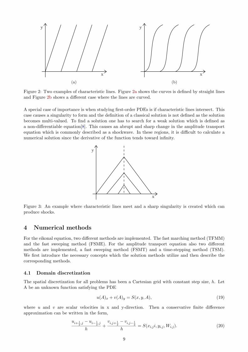
When the characteristic curves are found they can be pieced together to form a surface and usedwith boundary and/or initial condition to form a specific solution [8]. As the characteristic curves aredefined by the ODEs in equations (16) to (18) the curves can have different shapes. Figures 2a and2b show examples of characteristic curves. In Figure 2a an example is depicted, where the coefficientsare constant, and Figure 2b illustrates the case of variable coefficients. According to B.Engquist [11]the boundary for the eikonal and the amplitude transport equation should be defined in the sameregion as they share characteristic lines due to being derived from the same initial equation. He alsomentions the need to only prescribe the boundary condition at the inlet of the boundary and notprescribe the outlet.

8

y

x

(a)

y

x

(b)

Figure 2: Two examples of characteristic lines. Figure 2a shows the curves is defined by straight linesand Figure 2b shows a different case where the lines are curved.

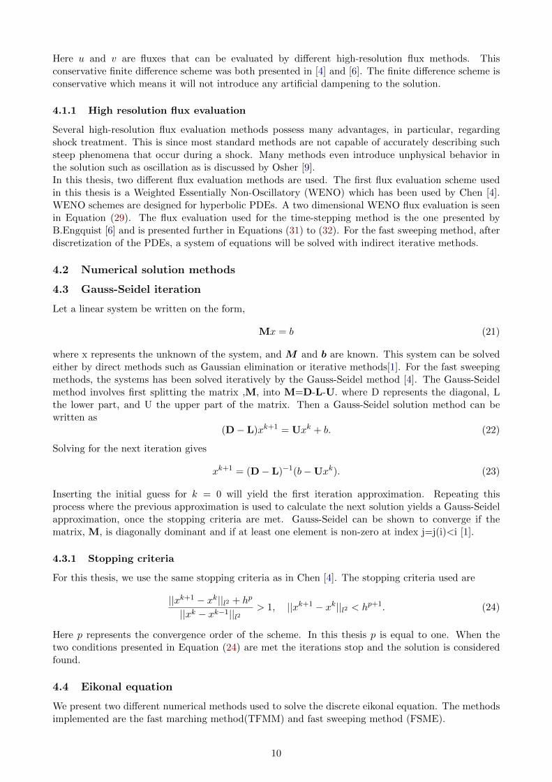
A special case of importance is when studying first-order PDEs is if characteristic lines intersect. Thiscase causes a singularity to form and the definition of a classical solution is not defined as the solutionbecomes multi-valued. To find a solution one has to search for a weak solution which is defined asa non-differentiable equation[8]. This causes an abrupt and sharp change in the amplitude transportequation which is commonly described as a shockwave. In these regions, it is difficult to calculate anumerical solution since the derivative of the function tends toward infinity.

y

x

Figure 3: An example where characteristic lines meet and a sharp singularity is created which canproduce shocks.

4 Numerical methods

For the eikonal equation, two different methods are implemented. The fast marching method (TFMM)and the fast sweeping method (FSME). For the amplitude transport equation also two differentmethods are implemented, a fast sweeping method (FSMT) and a time-stepping method (TSM).We first introduce the necessary concepts which the solution methods utilize and then describe thecorresponding methods.

4.1 Domain discretization

The spatial discretization for all problems has been a Cartesian grid with constant step size, h. LetA be an unknown function satisfying the PDE

u(A)x + v(A)y = S(x, y,A), (19)

where u and v are scalar velocities in x and y-direction. Then a conservative finite differenceapproximation can be written in the form,

ui+ 12,j − ui− 1

2,j

h+vi,j+ 1

2− vi,j− 1

2

h= S(xi,ji, yi,j ,Wi,j). (20)

9

Here u and v are fluxes that can be evaluated by different high-resolution flux methods. Thisconservative finite difference scheme was both presented in [4] and [6]. The finite difference scheme isconservative which means it will not introduce any artificial dampening to the solution.

4.1.1 High resolution flux evaluation

Several high-resolution flux evaluation methods possess many advantages, in particular, regardingshock treatment. This is since most standard methods are not capable of accurately describing suchsteep phenomena that occur during a shock. Many methods even introduce unphysical behavior inthe solution such as oscillation as is discussed by Osher [9].In this thesis, two different flux evaluation methods are used. The first flux evaluation scheme usedin this thesis is a Weighted Essentially Non-Oscillatory (WENO) which has been used by Chen [4].WENO schemes are designed for hyperbolic PDEs. A two dimensional WENO flux evaluation is seenin Equation (29). The flux evaluation used for the time-stepping method is the one presented byB.Engquist [6] and is presented further in Equations (31) to (32). For the fast sweeping method, afterdiscretization of the PDEs, a system of equations will be solved with indirect iterative methods.

4.2 Numerical solution methods

4.3 Gauss-Seidel iteration

Let a linear system be written on the form,

Mx = b (21)

where x represents the unknown of the system, and M and b are known. This system can be solvedeither by direct methods such as Gaussian elimination or iterative methods[1]. For the fast sweepingmethods, the systems has been solved iteratively by the Gauss-Seidel method [4]. The Gauss-Seidelmethod involves first splitting the matrix ,M, into M=D-L-U. where D represents the diagonal, Lthe lower part, and U the upper part of the matrix. Then a Gauss-Seidel solution method can bewritten as

(D− L)xk+1 = Uxk + b. (22)

Solving for the next iteration gives

xk+1 = (D− L)−1(b−Uxk). (23)

Inserting the initial guess for k = 0 will yield the first iteration approximation. Repeating thisprocess where the previous approximation is used to calculate the next solution yields a Gauss-Seidelapproximation, once the stopping criteria are met. Gauss-Seidel can be shown to converge if thematrix, M, is diagonally dominant and if at least one element is non-zero at index j=j(i)<i [1].

4.3.1 Stopping criteria

For this thesis, we use the same stopping criteria as in Chen [4]. The stopping criteria used are

||xk+1 − xk||l2 + hp

||xk − xk−1||l2> 1, ||xk+1 − xk||l2 < hp+1. (24)

Here p represents the convergence order of the scheme. In this thesis p is equal to one. When thetwo conditions presented in Equation (24) are met the iterations stop and the solution is consideredfound.

4.4 Eikonal equation

We present two different numerical methods used to solve the discrete eikonal equation. The methodsimplemented are the fast marching method(TFMM) and fast sweeping method (FSME).

10

4.4.1 Fast sweeping method

The idea of the fast sweeping method was first introduced in Zhao [14]. It is a PDE solving algorithmwhere the unique idea is to use Gauss-Seidel iteration from all different directions in the domain.According to Zhao each direction is meant to follow a group of characteristics lines. First, the eikonalequation (10) is discretized using a Godunov upwind finite difference scheme,

(φi,j −min(φi−1,j , φi+1,j))2 + (φi,j −min(φi,j−1, φi,j+1))2 = h2η2. (25)

Before using Gauss-Seidel to solve for the phase the next step is to introduce a=min(φki−1,j , φki+1,j)

and b=min(φi,j−1, φi,j+1) and express the phase as

φk+1i,j =

min(a, b) + hηi,j if |a− b| ≥ hηi,ja+b

√2η2i,jh

2−(a−b)2

2 if |a− b| < hηi,j .(26)

Where k denotes the current iteration of Gauss-Siedel. Initialize the solution with a large initial guess.The iteration is done in four different directions over the domain as our problem is in two dimensions[15]. The iterations stop when the solution φ satisfies the stopping criteria presented in Equation (24).The boundary condition in this thesis is a homogeneous Dirichlet boundary condition on the inlet ofthe domain, while the outlets are unprescribed. At the outlet where the boundary is unprescribed, aone-directional update is done per Zhao in [15]. These conditions would describe incoming wavefrontsfrom the inlet [11]. Proving stability of the discretization error is by many considered a difficult task.For this thesis the proofs presented by Zhao in [15] are considered reliable.

4.4.2 Fast marching method

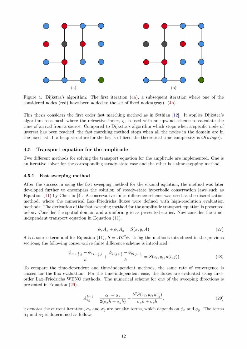
First pioneered by Sethian in [12], the fast marching method, is a computationally efficient methodof solving the eikonal equation. According to Sethian, one can think of the mesh as nodes on amathematical graph. As the phase, φ, can be considered the travel time from the source the solution forthe eikonal equation can be considered an optimization problem for finding the shortest path from thesource to all points. To find the shortest path when solving the eikonal solution, Dijkstra’s algorithmis often used. Dijkstra’s algorithm [5] is used to calculate the shortest travel distance between twonodes on a graph. To initialize the algorithm three lists are created. One for unconsidered nodes, onefor considered nodes, and one for fixed nodes. The next step is to add the starting points. For the fastmarching method this is the boundary to the list of fixed nodes with a value of zero. The remainingnodes are added to the list of unconsidered nodes with a travel distance set to infinity. The next stepis to calculate the travel distance of all the neighboring nodes in the set of fixed nodes and addingthe nodes to considered nodes with their respective travel distance. The node with the lowest traveldistance of all the considered nodes is added to the list of fixed nodes. Then the algorithm repeats bycalculating a new set of considered nodes around the new set of fixed nodes. This is repeated until thenode which one wants to calculate the distance from is encompassed in the fixed list. This iterationis illustrated in Figure 4 where the nodes in the fixed set are represented by gray, considered by red,unconsidered by blue, and the comparative node of interest with green.

11

(a) (b)

Figure 4: Dijkstra’s algorithm: The first iteration (4a), a subsequent iteration where one of theconsidered nodes (red) have been added to the set of fixed nodes(gray). (4b)

This thesis considers the first order fast marching method as in Sethian [12]. It applies Dijkstra’salgorithm to a mesh where the refractive index, η, is used with an upwind scheme to calculate thetime of arrival from a source. Compared to Dijkstra’s algorithm which stops when a specific node ofinterest has been reached, the fast marching method stops when all the nodes in the domain are inthe fixed list. If a heap structure for the list is utilized the theoretical time complexity is O(n logn).

4.5 Transport equation for the amplitude

Two different methods for solving the transport equation for the amplitude are implemented. One isan iterative solver for the corresponding steady-state case and the other is a time-stepping method.

4.5.1 Fast sweeping method

After the success in using the fast sweeping method for the eikonal equation, the method was laterdeveloped further to encompass the solution of steady-state hyperbolic conservation laws such asEquation (11) by Chen in [4]. A conservative finite difference scheme was used as the discretizationmethod, where the numerical Lax–Friedrichs fluxes were defined with high-resolution evaluationmethods. The derivation of the fast sweeping method for the amplitude transport equation is presentedbelow. Consider the spatial domain and a uniform grid as presented earlier. Now consider the time-independent transport equation in Equation (11).

φxAx + φyAy = S(x, y,A) (27)

S is a source term and for Equation (11), S = A∇2φ. Using the methods introduced in the previoussections, the following conservative finite difference scheme is introduced.

φxi+ 12,j − φxi− 1

2,j

h+φyi,j+ 1

2− φyi,j− 1

2

h= S(xi, yj , u(i, j)) (28)

To compare the time-dependent and time-independent methods, the same rate of convergence ischosen for the flux evaluation. For the time-independent case, the fluxes are evaluated using first-order Lax–Friedrichs WENO methods. The numerical scheme for one of the sweeping directions ispresented in Equation (29).

Ak+1i,j =

α1 + α2

2(σxh+ σyh)+h2S(xi, yj , u

mi,j)

σxh+ σyh, (29)

k denotes the current iteration, σx and σy are penalty terms, which depends on φx and φy. The termsα1 and α2 is determined as follows

12

α1 = σxh(Aki+1,j +Ak+1i−1,j) + σyh(Aki,j+1 +Ak+1

i,j−1)

α2 = h(φxAki+1,j − φxAk+1

i−1,j) + h(φyAki,j+1 − φyAk+1

i,j+1).

The method involves sweeping over the whole domain from all possible directions. For the 2D case,this gives a total of four directions. The discretization shown in Equation (29) sweeps from the leftand the bottom of the grid and ends at the right and top. As stated previously due to the amplitudetransport equation and eikonal equation sharing characteristic lines the boundary condition should bethe same. The inlet is prescribed while the outlet of the domain is not. As for the eikonal equation,a one-dimensional update is done on the unprescribed region.

4.5.2 Time-stepping method

B.Engquist shows in [6] a method to solve the time-dependent version of Equation (11). The domainfor the time-dependent solution is Ω with the additional dimension of time dimension, τ . The time isdivided into n points. Similarly, as in the time-independent problem, a finite-difference conservativescheme is introduced on the form.

An+1i,j = Ani,j −

(φxi+ 1

2,j − φxi− 1

2,j

h+φyi,j+ 1

2− φyi,j− 1

2

h

)+ S(xi, yj , u(i, j)) (30)

Instead of adding a term dependent on σ. B.Engquist in [6] defines the fluxes as,

φxi+ 12,j =

Ai,jnx if nx > 0

Ai+1,jnx if nx < 0φxi− 1

2,j =

Ai,jnx if nx > 0

Ai+1,jnx if nx < 0(31)

φyi,j+ 12

=

Ai,jnx if ny > 0

Ai,j+1nx if ny < 0φyi,j− 1

2=

Ai,jnx if ny > 0

Ai,j+1nx if ny < 0(32)

where n is defined by the gradient of the velocity field. To ensure numerical stability of the solutionthe discretization needs to follow the CFL condition for a two dimensional case, presented in Equation(33),

CFL =∆tφxh

+∆tφyh≤ 1. (33)

5 Computer specifications and implementation

All runs are done on a Lenovo computer. With a Intel(R) Core(TM) i7-7500U CPU @ 2.70GHz coreusing Ubuntu 18.04 with a x86 64 architecture. The software used was python 3.7.6. To increase theperformance of the code for the steady-state method Numba Just-in-time (Jit) python compiler hasbeen used to reduce the run time. Numba increases performance by compiling it to machine code“just-in-time” for execution. Parts of the code can then run at almost native machine code speed.

6 Numerical results

This section will present the numerical results of the four tested methods of solving the eikonal andamplitude transport equation. The methods which have been tested are a fast sweeping method and thefast marching method for the eikonal equation. For the amplitude transport equation, a fast sweepingmethod for a steady-state hyperbolic equation is implemented and also a time stepping method. Thegrid for all numerical methods implemented is uniform. The first subsection defines the input dataand boundary conditions used to produce the results. As it is of interest to have a solver that canproduce results quickly the performance of the different methods has been measured in terms of runtime. Additionally, the discretization error has been measured to determine the convergence rate. Thediscretization error has been measured in terms of absolute error, and the l2-norm. Finally, the lastsection covers the solutions of the equations for several cases.

13

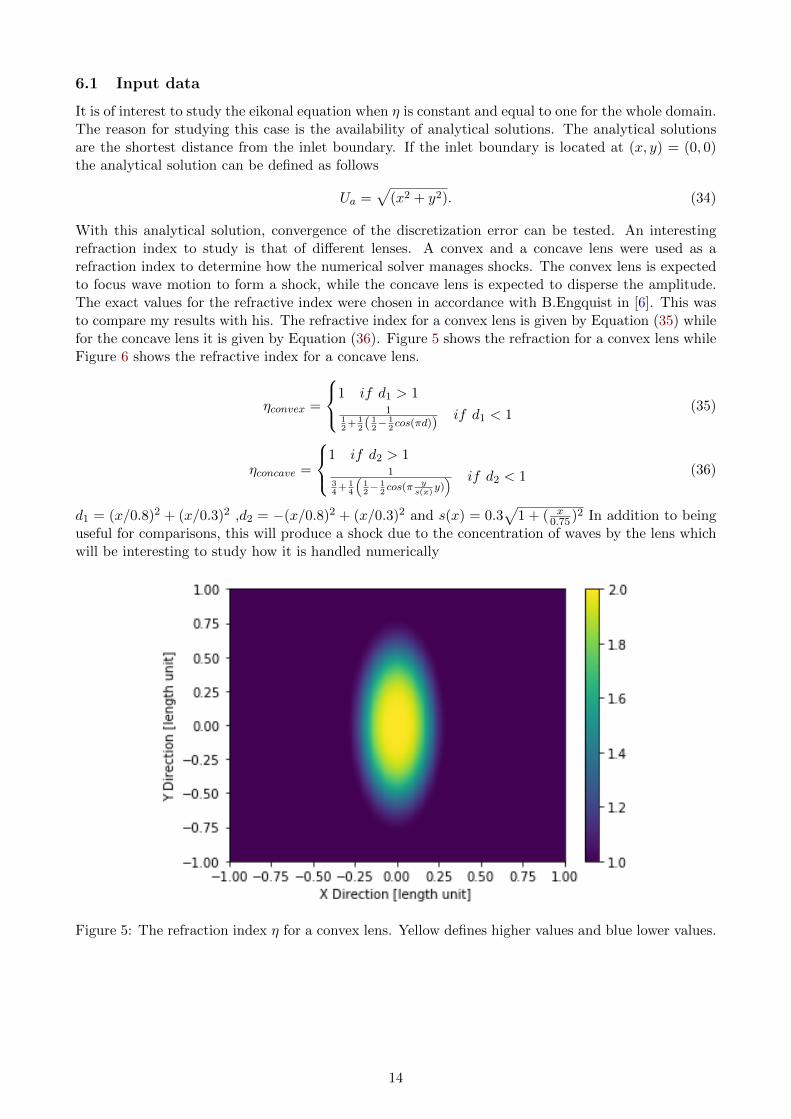
6.1 Input data

It is of interest to study the eikonal equation when η is constant and equal to one for the whole domain.The reason for studying this case is the availability of analytical solutions. The analytical solutionsare the shortest distance from the inlet boundary. If the inlet boundary is located at (x, y) = (0, 0)the analytical solution can be defined as follows

Ua =√

(x2 + y2). (34)

With this analytical solution, convergence of the discretization error can be tested. An interestingrefraction index to study is that of different lenses. A convex and a concave lens were used as arefraction index to determine how the numerical solver manages shocks. The convex lens is expectedto focus wave motion to form a shock, while the concave lens is expected to disperse the amplitude.The exact values for the refractive index were chosen in accordance with B.Engquist in [6]. This wasto compare my results with his. The refractive index for a convex lens is given by Equation (35) whilefor the concave lens it is given by Equation (36). Figure 5 shows the refraction for a convex lens whileFigure 6 shows the refractive index for a concave lens.

ηconvex =

1 if d1 > 11

12

+ 12( 1

2− 1

2cos(πd))

if d1 < 1(35)

ηconcave =

1 if d2 > 11

34

+ 14

(12− 1

2cos(π y

s(x)y)) if d2 < 1 (36)

d1 = (x/0.8)2 + (x/0.3)2 ,d2 = −(x/0.8)2 + (x/0.3)2 and s(x) = 0.3√

1 + ( x0.75)2 In addition to being

useful for comparisons, this will produce a shock due to the concentration of waves by the lens whichwill be interesting to study how it is handled numerically

Figure 5: The refraction index η for a convex lens. Yellow defines higher values and blue lower values.

14

Figure 6: The refraction index η for a concave lens. Yellow defines higher values and blue lower values.

The solutions to the amplitude transport equation have been calculated from the numerical value of φfrom the data for η from Section 6.1. To test the convergence of the solvers for the amplitude transportequation an analytical solution is manufactured. The manufactured solution is done following Roachein [10]. The manufactured analytical solution can be found if you start by defining φx = 1 and φy = 1,the PDE can then be written as,

dA

dx+dA

dy= 0 (37)

Assume a general solution on this form in Equation (38)

A(x, y) = arctan

(x− y0.1

)(38)

With this manufactured solution a source term for this case has to be calculated by inserting thegeneral solution into Equation (37).

dA

dx+dA

dy= S(x, y,A) (39)

The source term, in this case, is equal to zero as the two derivatives cancel out. The boundary is setto the analytical solution on the inlet boundary. The inlet boundary is on the left of the domain ΓLand the bottom ΓB. Another analytical solution for the steady state transport equation is presented

in Equation (40). This when φx = 1 and φy = 1 and in the inflow the boundary ΓL = e−(x−0.5r∗

)2 .

Aa = e−(x−y−0.5r∗

)2 (40)

.

6.2 Performance

The run time was defined as the time used by the numerical solver. The time was measured usingpythons time module, the program was then run three times to produce an average time which ispresented here. The fast sweeping methods were implemented both with and without the Jit compiler.Here the results which have been optimized with the Jit compiler are indicated by an ”O” ending. Ifthe run time exceeded three hours the run time was not considered, as we strive towards a fast solver.The three hours mark was determined arbitrarily.

15

6.2.1 Eikonal equation

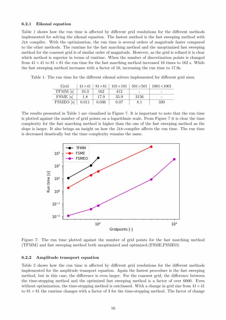
Table 1 shows how the run time is affected by different grid resolutions for the different methodsimplemented for solving the eikonal equation. The fastest method is the fast sweeping method withJit compiler. With the optimization, the run time is several orders of magnitude faster comparedto the other methods. The runtime for the fast marching method and the unoptimized fast sweepingmethod for the coarsest grid is of similar order of magnitude. However, as the grid is refined it is clearwhich method is superior in terms of runtime. When the number of discretization points is changedfrom 41× 41 to 81× 81 the run time for the fast marching method increased 16 times to 162 s. Whilethe fast sweeping method increases with a factor of 10, increasing the run time to 17.9s.

Table 1: The run time for the different eikonal solvers implemented for different grid sizes.

Grid 41×41 81×81 101×101 501×501 1001×1001

TFMM [s] 10.3 162 412 - -

FSME [s] 1.8 17.9 35.9 3156 -

FSMEO [s] 0.011 0.036 0.07 8.1 330

The results presented in Table 1 are visualized in Figure 7. It is important to note that the run timeis plotted against the number of grid points on a logarithmic scale. From Figure 7 it is clear the timecomplexity for the fast marching method is higher than the one of the fast sweeping method as theslope is larger. It also brings an insight on how the Jit-compiler affects the run time. The run timeis decreased drastically but the time complexity remains the same.

Figure 7: The run time plotted against the number of grid points for the fast marching method(TFMM) and fast sweeping method both unoptimized and optimized.(FSME,FSMEO)

6.2.2 Amplitude transport equation

Table 2 shows how the run time is affected by different grid resolutions for the different methodsimplemented for the amplitude transport equation. Again the fastest procedure is the fast sweepingmethod, but in this case, the difference is even larger. For the coarsest grid, the difference betweenthe time-stepping method and the optimized fast sweeping method is a factor of over 6000. Evenwithout optimization, the time-stepping method is outclassed. With a change in grid size from 41×41to 81× 81 the runtime changes with a factor of 3 for the time-stepping method. The factor of change

16

for the sweeping method is approximately 3.8. In terms of time complexity, the time-stepping methodperformed better.

Table 2: The runtime for different grid resolutions for the amplitude transport equation solvers.

Grid 41×41 81×81 101×101 501×501 1001×1001

TSM [s] 10.9 32.2 57.46 - -

FSMT [s] 0.067 0.26 0.519 10.3 46.8

FSMTO [s] 0.0018 0.0025 0.0034 0.092 0.88

The results presented in Table 2 is visualized in Figure 8. Figure 8 highlights the effect the Jit-compiler has on run time, the time complexity remains mostly the same regardless.

Figure 8: The runtime plotted against the number of grid points for the time stepping method(TSM)and the fast sweeping method both unoptimized and optimized(FSMT,FSMTO).

6.3 Convergence

This section covers the study of convergence of the discretization error for the numerical methods.There are many different ways in which one can analyze the discretization error. Two commonmethods of defining errors have been implemented and used to analyze the convergence propertiesfor the numerical solvers. The first one is a single point of absolute error. This error is measuredpoint-wise and is defined in Equation (41).

Error ≡√

(Ua − U)2, (41)

The second way used was the discrete l2-norm which is defined as follows,

l2(Ua − U) ≡√h∑

Ω

|Ua − U |2. (42)

This error analysis was done for all the methods implemented. The convergence was tested againstknown analytical solutions for each case. It is of great interest to know the rate at which the solutionconverges. Let, q, be the convergence rate and define it as in Equation (43).

q ≡ log10(||Ua − U (n1)||||Ua − U (n2)||

)/log10(n1

n2) (43)

The expected convergence rate is one for all methods.

17

6.3.1 Eikonal equation

Table 3 and 4 show the discretization error computed with the different methods introduced in Section6.3. Table 3 shows how the absolute error changes with respect to grid size for the fast marchingmethod and the fast sweeping method. In addition the tables show the convergence rate. When theabsolute error was measured it was done at the same x- and y-coordinates for both methods. Interms of absolute error, both methods show a convergence rate close to one which is the expectedvalue. The convergence rate and absolute error are the same up to the third decimal for both the fastsweeping method and the fast marching method. For the fast sweeping method with a coarse grid,the convergence rate is lower than one. Table 4 shows how the l2-norm and convergence rate changeswith respect to the grid size. The convergence rate is closer to 1 for the fast sweeping method thanfor the fast marching method. The convergence rate for the fast marching method ranges between 0.5and 0.7. While the convergence rate for the fast sweeping method starts at 0.7 and increases as yourefine the grid.

Table 3: Decimal logarithm of discretization error and convergence rate, q, using the absolute error.

Grid 41×41 81×81 101×101 501×501 1001×1001

TFMM -1.834 -2.135 -2.232 - -

q 1.000 1.000 - -

FSME -1.834 -2.135 -2.232 -2.931 -3.232

q 1.000 1.000 1.000 1.000

Table 4: Decimal logarithm of discretization error and convergence rate, q, using the l2-norm.

Grid 41×41 81×81 101×101 501×501 1001×1001

TFMM -1.360 -1.578 -1.638 - -

q - 0.736 0.627 - -

FSME -1.182 -1.400 -1.472 -2.013 -2.257

q - 0.725 0.741 0.774 0.811

Figure 9 and 10 show the numerical solution to the eikonal equation in red and the analytical solutionin black. Figure 9 shows the solution from the fast marching method and Figure 10 shows the solutionfrom the fast sweeping method. The coarsest grid for both methods was 21× 21 illustrated in Figure9a and 10a. Both methods for this case produce a larger error along the axis of the domain. As thegrid is refined the error reduces drastically. In Figure 9b the result from the fast marching method fora grid of size 101 × 101 is shown. In Figure 10b the result from the fast sweeping method for a gridof size 1001× 1001 is shown. With this grid resolution, the error is minuscule.

(a) Contour map with a grid of 21× 21 (b) Contour map with a grid of 101× 101

Figure 9: Shows the analytical and numerical solution of the eikonal equation by the fast marchingmethod. The inlet boundary is a point source in the center.

18

(a) Contour map with a grid of 21× 21 (b) Contour map with a grid of 1001× 1001

Figure 10: Shows the analytical and numerical solution of the eikonal equation by the fast sweepingmethod. The inlet boundary is a point source in the center.

6.3.2 Amplitude transport equation

Table 5 and 6 show the discretization error computed with the different methods introduced in section6.3. Table 5 shows how the absolute error changes with respect to grid size for the fast sweeping methodand the time-stepping method. In addition, it shows the convergence rate. When the absolute errorwas measured it was done at the same x- and y-coordinates for both methods. For both methods interms of the absolute error, the convergence rate is close to one, which is the expected value. Theconvergence rate and absolute error are very similar for both the fast sweeping method and the time-stepping method. Table 6 shows how the l2-norm and convergence rate changes with respect to thegrid size. For the l2-norm the two methods are again similar to each other. The rate of convergence forboth methods are lower than one, starting from approximately 0.5. For the fast sweeping method theconvergence rate increases as you refine the mesh, For the time-stepping method, it is not possible toconclude the behavior for larger grid sizes. The time-stepping method was solved for a very small timestep in the results presented here. This was to reduce the error introduced by the time discretizationbut also satisfy the CFL-condition. The final time was set high to 700 with 10000-time steps. Thefinal time was to ensure a comparability with the steady-state solver.

Table 5: Decimal logarithm of discretization error and convergence rate, q, using the absolute error

Grid 41×41 81×81 101×101 501×501 1001×1001

FSMT -1.483 -1.763 -1.857 -2.544 -2.843

q 0.931 0.960 0.983 0.995

TSM -1.612 -1.894 -1.986 - -

q 0.936 0.949 - -

Table 6: Decimal logarithm of discretization error and convergence rate, q, using the l2-norm

Grid 41×41 81×81 101×101 501×501 1001×1001

FSMT -0.264 -0.420 -0.474 -0.925 -1.155

q 0.519 0.557 0.646 0.764

TSM -0.295 -0.453 -0.507 - -

q 0.524 0.559 - -

Figure 11 depicts a slice of the numerical and analytical solution by both the time-stepping methodand the fast sweeping method. Figure 11a shows the results done by the fast sweeping method andFigure 11b the results for the time-stepping method. The legend names are referring to the numberof grid points, n, in the n× n grid. When n = 1001 the numerical and analytical solution are almostindistinguishable. This is seen in Figure 11a. Even the finest grid tested for the time-stepping method

19

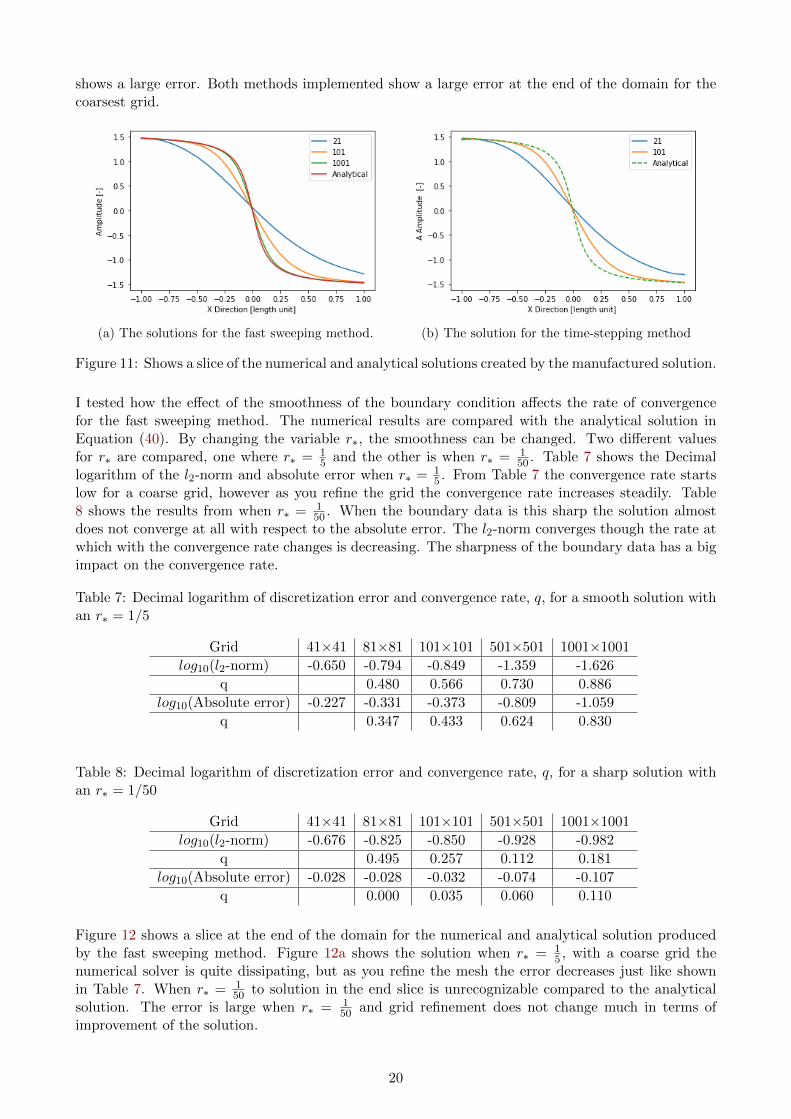
shows a large error. Both methods implemented show a large error at the end of the domain for thecoarsest grid.

(a) The solutions for the fast sweeping method. (b) The solution for the time-stepping method

Figure 11: Shows a slice of the numerical and analytical solutions created by the manufactured solution.

I tested how the effect of the smoothness of the boundary condition affects the rate of convergencefor the fast sweeping method. The numerical results are compared with the analytical solution inEquation (40). By changing the variable r∗, the smoothness can be changed. Two different valuesfor r∗ are compared, one where r∗ = 1

5 and the other is when r∗ = 150 . Table 7 shows the Decimal

logarithm of the l2-norm and absolute error when r∗ = 15 . From Table 7 the convergence rate starts

low for a coarse grid, however as you refine the grid the convergence rate increases steadily. Table8 shows the results from when r∗ = 1

50 . When the boundary data is this sharp the solution almostdoes not converge at all with respect to the absolute error. The l2-norm converges though the rate atwhich with the convergence rate changes is decreasing. The sharpness of the boundary data has a bigimpact on the convergence rate.

Table 7: Decimal logarithm of discretization error and convergence rate, q, for a smooth solution withan r∗ = 1/5

Grid 41×41 81×81 101×101 501×501 1001×1001

log10(l2-norm) -0.650 -0.794 -0.849 -1.359 -1.626

q 0.480 0.566 0.730 0.886

log10(Absolute error) -0.227 -0.331 -0.373 -0.809 -1.059

q 0.347 0.433 0.624 0.830

Table 8: Decimal logarithm of discretization error and convergence rate, q, for a sharp solution withan r∗ = 1/50

Grid 41×41 81×81 101×101 501×501 1001×1001

log10(l2-norm) -0.676 -0.825 -0.850 -0.928 -0.982

q 0.495 0.257 0.112 0.181

log10(Absolute error) -0.028 -0.028 -0.032 -0.074 -0.107

q 0.000 0.035 0.060 0.110

Figure 12 shows a slice at the end of the domain for the numerical and analytical solution producedby the fast sweeping method. Figure 12a shows the solution when r∗ = 1

5 , with a coarse grid thenumerical solver is quite dissipating, but as you refine the mesh the error decreases just like shownin Table 7. When r∗ = 1

50 to solution in the end slice is unrecognizable compared to the analyticalsolution. The error is large when r∗ = 1

50 and grid refinement does not change much in terms ofimprovement of the solution.

20

(a) Slices of the solution for different grid sizeswith r∗ = 1/5

(b) Slices of the solution for different grid sizeswith r∗ = 1/50

Figure 12: Numerical and analytical solution to the amplitude transport equation when the boundarycondition is a Gaussian impulse

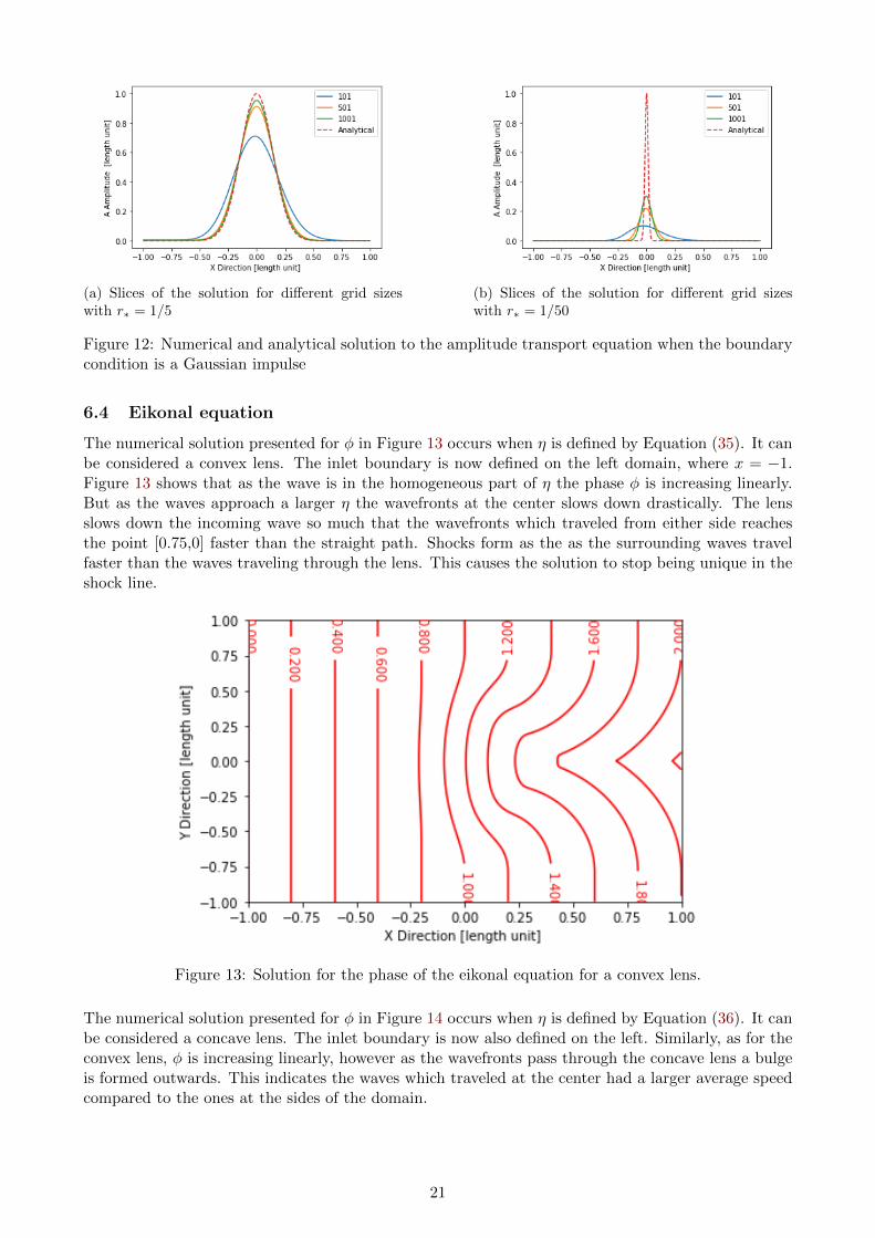
6.4 Eikonal equation

The numerical solution presented for φ in Figure 13 occurs when η is defined by Equation (35). It canbe considered a convex lens. The inlet boundary is now defined on the left domain, where x = −1.Figure 13 shows that as the wave is in the homogeneous part of η the phase φ is increasing linearly.But as the waves approach a larger η the wavefronts at the center slows down drastically. The lensslows down the incoming wave so much that the wavefronts which traveled from either side reachesthe point [0.75,0] faster than the straight path. Shocks form as the as the surrounding waves travelfaster than the waves traveling through the lens. This causes the solution to stop being unique in theshock line.

Figure 13: Solution for the phase of the eikonal equation for a convex lens.

The numerical solution presented for φ in Figure 14 occurs when η is defined by Equation (36). It canbe considered a concave lens. The inlet boundary is now also defined on the left. Similarly, as for theconvex lens, φ is increasing linearly, however as the wavefronts pass through the concave lens a bulgeis formed outwards. This indicates the waves which traveled at the center had a larger average speedcompared to the ones at the sides of the domain.

21

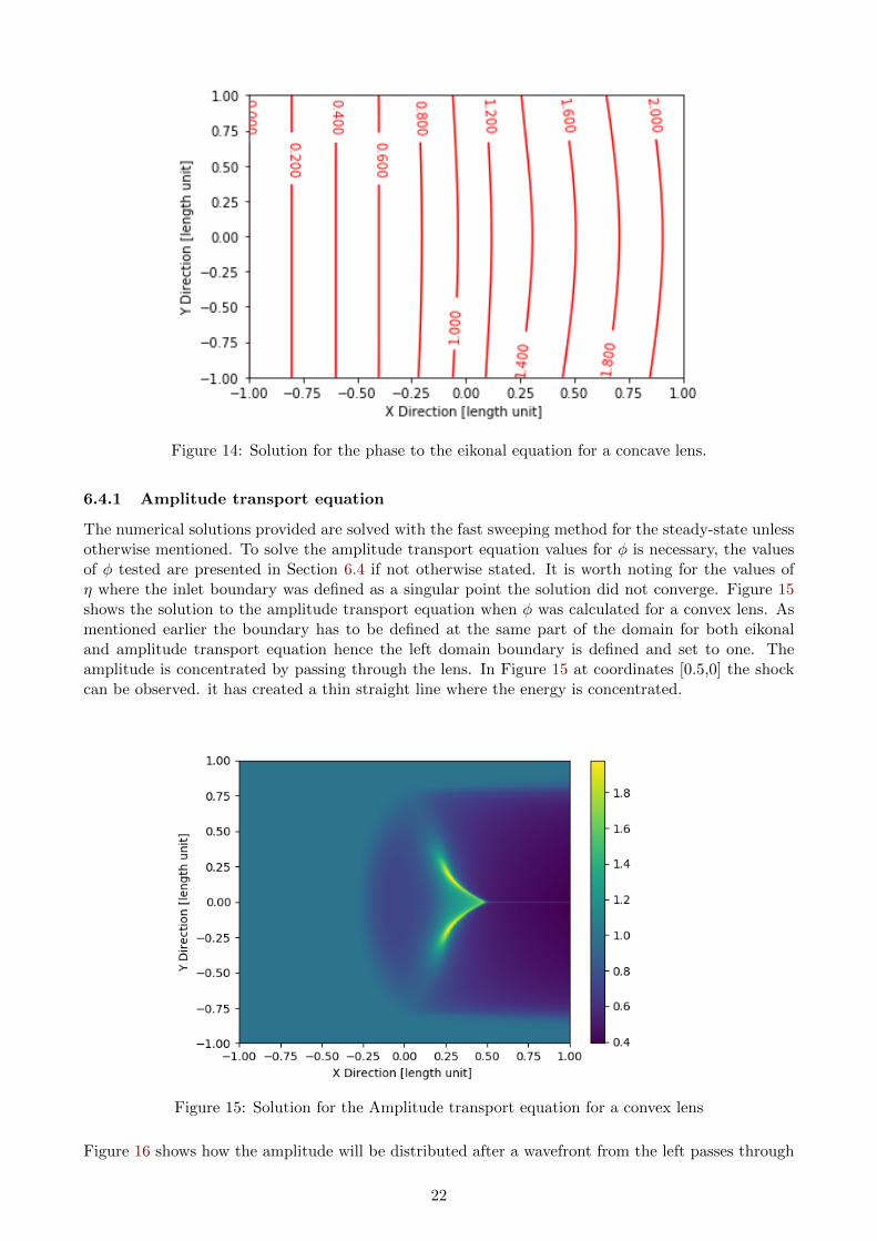
Figure 14: Solution for the phase to the eikonal equation for a concave lens.

6.4.1 Amplitude transport equation

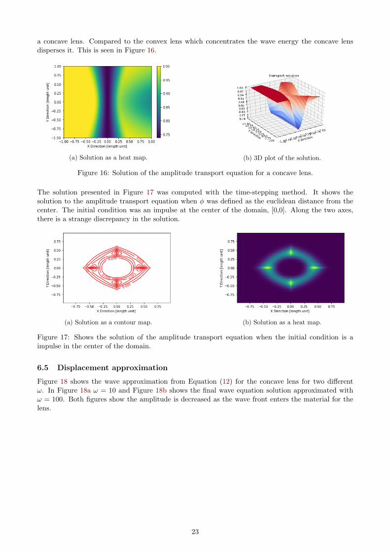
The numerical solutions provided are solved with the fast sweeping method for the steady-state unlessotherwise mentioned. To solve the amplitude transport equation values for φ is necessary, the valuesof φ tested are presented in Section 6.4 if not otherwise stated. It is worth noting for the values ofη where the inlet boundary was defined as a singular point the solution did not converge. Figure 15shows the solution to the amplitude transport equation when φ was calculated for a convex lens. Asmentioned earlier the boundary has to be defined at the same part of the domain for both eikonaland amplitude transport equation hence the left domain boundary is defined and set to one. Theamplitude is concentrated by passing through the lens. In Figure 15 at coordinates [0.5,0] the shockcan be observed. it has created a thin straight line where the energy is concentrated.

Figure 15: Solution for the Amplitude transport equation for a convex lens

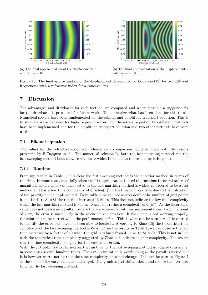
Figure 16 shows how the amplitude will be distributed after a wavefront from the left passes through

22

a concave lens. Compared to the convex lens which concentrates the wave energy the concave lensdisperses it. This is seen in Figure 16.

(a) Solution as a heat map. (b) 3D plot of the solution.

Figure 16: Solution of the amplitude transport equation for a concave lens.

The solution presented in Figure 17 was computed with the time-stepping method. It shows thesolution to the amplitude transport equation when φ was defined as the euclidean distance from thecenter. The initial condition was an impulse at the center of the domain, [0,0]. Along the two axes,there is a strange discrepancy in the solution.

(a) Solution as a contour map. (b) Solution as a heat map.

Figure 17: Shows the solution of the amplitude transport equation when the initial condition is aimpulse in the center of the domain.

6.5 Displacement approximation

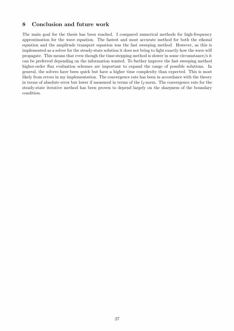
Figure 18 shows the wave approximation from Equation (12) for the concave lens for two differentω. In Figure 18a ω = 10 and Figure 18b shows the final wave equation solution approximated withω = 100. Both figures show the amplitude is decreased as the wave front enters the material for thelens.

23

(a) The final approximation of the displacement uwith an ω = 10

(b) The final approximation of the displacement uwith an ω = 100

Figure 18: The final approximation of the displacement determined by Equation (12) for two differentfrequencies with a refractive index for a concave lens.

7 Discussion

The advantages and drawbacks for each method are compared and where possible a suggested fixfor the drawbacks is presented for future work. To summarize what has been done for this thesis.Numerical solvers have been implemented for the eikonal and amplitude transport equation. This isto simulate wave behavior for high-frequency waves. For the eikonal equation two different methodshave been implemented and for the amplitude transport equation and two other methods have beenused.

7.1 Eikonal equation

The values for the refractive index were chosen so a comparison could be made with the resultspresented by B.Engquist in [6]. The numerical solution by both the fast marching method and thefast sweeping method both show results for φ which is similar to the results by B.Engquist.

7.1.1 Runtime

From my results in Table 1, it is clear the fast sweeping method is the superior method in terms ofrun time. In some cases, especially when the Jit optimization is used the run time is several orders ofmagnitude faster. This was unexpected as the fast marching method is widely considered to be a fastmethod and has a low time complexity of O(n log(n)). This time complexity is due to the utilizationof the priority queue implemented. From table 1 we can see as you double the number of grid pointsfrom 41×41 to 81×81 the run time increases 16 times. This does not indicate the low time complexitywhich the fast marching method is known to have but rather a complexity of O(n4). As the theoreticalvalue does not match my results I believe there was an error with my implementation. From my pointof view, the error is most likely in the queue implementation. If the queue is not working properlythe solution can be correct while the performance suffers. This is what can be seen here. I have triedto identify the error but have not been able to locate it. According to Zhao [15] the theoretical timecomplexity of the fast sweeping method is O(n). From the results in Table 1, we can observe the runtime increases by a factor of 10 when the grid is refined from 41 × 41 to 81 × 81. This is not in linewith the theoretical time complexity suggested by Zhao but indicates higher complexity. The reasonwhy the time complexity is higher for this case is uncertain.With the Jit optimization turned on, the run time for the fast sweeping method is reduced drastically,in some cases several hundred times. The Jit optimization is worth doing as the payoff is incredible.It is however worth noting that the time complexity does not change. This can be seen in Figure 7as the slope of the curve remains unchanged. The graph is just shifted down and reduce the overheadtime for the fast sweeping method.

24

To examine the fairness of the comparison of the run time for the two methods. It can be consideredunfair to compare an iterative method with a non-iterative method. As the fast sweeping method isiterative the run time can depend largely on the initial guess as well as the values of the refractiveindex η. While, the run time of the fast marching method will be more constant no matter thecircumstances. Still it is important to know the fastest method. The property of depending on theinitial guess could potentially be utilized in future work to an advantage to reduce the run time, ifyou were to solve for a coarse grid first and then use the solution as a initial guess for a finer meshthere is a possibility of a performance boost.There are several ways to improve the run time for the fast marching method I implemented. Thefirst would be to correct the error regarding the time complexity. This has the potential to reduce therun time drastically and could make the method competitive with the fast sweeping method or evenoutperform it. One could also look into the method proposed by Yatziv [13] as this is using an untidypriority queue and can reduce the time complexity to O(n).

7.1.2 Convergence

The results in Table 3 show the absolute error to be the same value for both methods. That surprisedme as I assumed there be a difference. If it were not for two reasons, the results being so similar wouldbe a possible indication of an error. The first reason, the theoretical and experimental convergencerate match. Second, the results in Table 4 shows a different l2-norm which indicates a difference inthe methods. Though as can be seen in Figure 9 the error is largest along the axis for both caseswhich makes me believe the underlying mechanics of numerical solvers are very similar. From Table 4we can also observe that the convergence rate for my implementation in terms of the l2-norm is lowerthan the expected rate of one. A possible reason why it is lower than expected is whether or not mydefinition of the discrete l2-norm in Equation (42) is correct especially considering the two-dimensionalcase. Another possible reason for this is the fact that the edges of the domain are calculated with aone sides difference as presented in Zhao [15]. This could explain why the absolute error evaluated ata point has the expected convergence rate while the l2-norm considering the entire domain is affected.It is also observed that for the fast marching method the convergence rate does not seem to changemuch when the grid is refined. For the fast sweeping method, the convergence rate does however climbcloser to the expected value of one as you refine the grid. For the fast sweeping method implementedfor the steady-state conservation laws in Chen [4] the convergence rate in some cases started lowerthan the expected value, but increased as you refined the mesh. Chen mentions this to be a propertyof the discretization method used, as it is more dissipating for coarse grids. Something similar couldbe happening for the fast sweeping method.

7.2 Amplitude transport equation

The exact values of the refractive index for the convex and the concave lens was chosen so the numericalsolution for the phase φ and the amplitude A could be compared to the results by B.Engquist in [6].The results in Figure 15 and 16 is comparable with the results produced by B.Engquist. It is a goodsign that the time-dependent method, implemented by B.Engquist, produces similar results as thesteady state solution solved by the fast sweeping method implemented for this thesis.The numerical results can also be compared to the intuition from optics. According to Snell’s law ofrefraction as light travels from material A to B the angle of incidence is larger than the of refractionif ηA > ηB. The numerical solution for the convex lens shows this behavior. The wavefront is beingfocused after passing through the region of higher refractive index.An Improvement which can be done for the calculation of the amplitude is to include more term fromthe infinite sum of ray series approximation. As previously mentioned according to Johana in [3] thefirst term is usually enough for seismology, but if we want to model diffraction patterns more termsin the infinite sum has to be included.As mentioned in the results some numerical values for φ were not used to calculate the amplitude.The values for φ, which was not considered, is when the inlet boundary was a singular point. Whenthe inlet is defined only in a singular point the solvers for the amplitude transport equation do not

25

converge. I believe this is due to the numerical flux schemes implemented. The convergence rate isonly of the first order, which is not capable of handling such a sharp change. The exact effect of thesharpness of the inlet boundary is further discussed in Section 7.2.2.In seismic, it can be of interest to model the solution when the inlet of the domain is a singular point,as this could model an explosion in bedrock. An improvement to encompass cases with a singularpoint boundary would be to implement higher-order flux discretization. Higher-order WENO-schemesare presented in Chen [4]. As mentioned earlier it is important to remember even though this wouldmake it possible to solve for different cases the final error for the displacement might be unaffectedas it is dependent on several numerical solvers in sequence. The method with the lowest convergencerate will determine the convergence rate of the system as a whole.The effect of a point inlet boundary for the time-stepping method is shown in Figure 17. Thediscrepancies along the axis can be seen, I believe this is also due to the order of convergence ofthe numerical scheme. Improving this could potentially remove this error.For most cases, a steady-state solution is sufficient to describe the wave movement, unless there is aneed for precise behavior in the time domain. So the steady-state solver gives less information aboutthe wave behavior in total but is several orders of magnitude faster so there is a trade-off.

7.2.1 Run time

From Table 2 the run time for the fast sweeping method and the time-stepping method is shown.Similarly, as for solving the eikonal equation, the fast sweeping method is far superior to the comparingmethod. It is expected that the fast sweeping method will have a better performance as it solves forthe steady-state and disregard the time dimension. The time complexity however is lower for thetime-stepping method compared to the fast sweeping method. For this case it is quite irrelevant asit is so slow. Table 2 highlights one major drawback of the time-stepping method. We can observeempty rows for finer grid sizes. Either the run time was too large or the size of the matrix createdwas several GB in size and the computer used was not capable of solving it. The size of the matrixwas very large as the number of time steps was set high both to satisfy the CFL-condition and tominimize the effect the time discretization has on the error.

7.2.2 Convergence

The fast sweeping method and the time-stepping method were both tested against the manufacturedanalytical solution presented in Equation (38). The results are presented in Table 5 and 6. For theabsolute error the convergence rate is very close to one, the expected convergence rate. However, theconvergence rate for the l2-norm is lower than expected. The convergence rate is increasing for thefast sweeping method as the grid is refined. One reason for this can be the dissipating properties forWENO-fluxes as mentioned in Zhao [15]. The effect of the smoothness of the boundary condition forthe steady-state amplitude transport equation was tested. The results for the is presented in Table7 and Table 8. The convergence rate for the sharp boundary condition is very low. The convergencerate is close to zero and sometimes negative indicating the solution almost not converging. This isbelieved to be the reason why if the boundary is defined in a singular inlet point the solution notconverging at all.

26

8 Conclusion and future work

The main goal for the thesis has been reached. I compared numerical methods for high-frequencyapproximation for the wave equation. The fastest and most accurate method for both the eikonalequation and the amplitude transport equation was the fast sweeping method. However, as this isimplemented as a solver for the steady-state solution it does not bring to light exactly how the wave willpropagate. This means that even though the time-stepping method is slower in some circumstance/s itcan be preferred depending on the information wanted. To further improve the fast sweeping methodhigher-order flux evaluation schemes are important to expand the range of possible solutions. Ingeneral, the solvers have been quick but have a higher time complexity than expected. This is mostlikely from errors in my implementation. The convergence rate has been in accordance with the theoryin terms of absolute error but lower if measured in terms of the l2-norm. The convergence rate for thesteady-state iterative method has been proven to depend largely on the sharpness of the boundarycondition.

27

References

[1] Owe Axelsson. Iterative Solution Methods. Cambridge University Press, 1994. doi: 10.1017/CBO9780511624100.

[2] K. Y. Billah and Robert H. Scanlan. “Resonance, Tacoma Narrows bridge failure, and undergraduatephysics textbooks”. English. In: American journal of physics 59.2 (1991), pp. 118–124.

[3] Johana Brokesova. ASYMPTOTIC RAY METHOD IN SEISMOLOGY-A TUTORIAL. MATFYZPRESS,2006. isbn: 80-86732-74-6.

[4] Weitao Chen, Ching-Shan Chou, and Chiu-Yen Kao. “Lax–Friedrichs fast sweeping methods forsteady state problems for hyperbolic conservation laws”. In: Journal of Computational Physics234 (2013), pp. 452–471.

[5] E.W. DIJKSTRA. “A Note on Two Problems in Connexion with Graphs.” In: NumerischeMathematik 1 (1959), pp. 269–271. url: http://eudml.org/doc/131436.

[6] B.Engquist E.Fatemi and S. Osher. “Numerical Solution of the High Frequency AsymptoticExpansion for the Scalar Wave Equation”. In: Journal of Computational Physics 120 (Aug.1995), pp. 145–155. doi: https://doi.org/10.1006/jcph.1995.1154.

[7] Richard haberman. Applied partial differential equations with fourier seriers and boundary valueproblem. 5th ed. Edinburgh Gate, Harlow, Essex CM20 2JE, England: Pearson, 2014.

[8] Math 220A, Partial Differential Equations of Applied Mathematics. Fall 2002. eprint: https://web.stanford.edu/class/math220a/handouts/.

[9] Stanley Osher et al. “Weighted Essentially Non-Oscillatory Schemes”. In: (1994).

[10] Patrick J. Roache. “Code Verification by the Method of Manufactured Solutions ”. In: Journalof Fluids Engineering 124.1 (Nov. 2001), pp. 4–10. issn: 0098-2202. doi: 10.1115/1.1436090.eprint: https://asmedigitalcollection.asme.org/fluidsengineering/article-pdf/124/1/4/5901562/4\_1.pdf. url: https://doi.org/10.1115/1.1436090.

[11] Olof Runborg. Numerical Solutions of Differential Equations. Spring 2012.

[12] J A Sethian. “A fast marching level set method for monotonically advancing fronts”. In: Proceedingsof the National Academy of Sciences 93.4 (1996), pp. 1591–1595. issn: 0027-8424. doi: 10.1073/pnas.93.4.1591. eprint: https://www.pnas.org/content/93/4/1591.full.pdf. url:https://www.pnas.org/content/93/4/1591.

[13] Liron Yatziv, Alberto Bartesaghi, and Guillermo Sapiro. “O(N) implementation of the fastmarching algorithm”. In: Journal of Computational Physics 212.2 (2006), pp. 393–399. issn:0021-9991. doi: https://doi.org/10.1016/j.jcp.2005.08.005. url: http://www.

sciencedirect.com/science/article/pii/S0021999105003736.

[14] Hong-Kai Zhao et al. “Implicit and Nonparametric Shape Reconstruction from UnorganizedData Using a Variational Level Set Method”. In: Computer Vision and Image Understanding80.3 (2000), pp. 295–314. issn: 1077-3142. doi: https://doi.org/10.1006/cviu.2000.0875.url: http://www.sciencedirect.com/science/article/pii/S1077314200908750.

[15] Hongkai Zhao. “A FAST SWEEPING METHOD FOR EIKONAL EQUATIONS”. In: (2004).

28