ENTE PER LE NUOVE TECNOLOGIEL'ENERGIA E L'AMBIENTE " |foi00038

Dipartimento Innovazione

ISSN/ 1120/5571

NUMERICAL SIMULATION OF TIG WELDINGWITH FILLER OF STEEL PIECES

OF HIGH THICKNESS

B. CARMIGNANI, G. TOSELLI

ENEA - Dipartimento InnovazioneCentra Ricerche "Ezio Clementel", Bologna

RT/INN/99/16

Work presented at the 12th International ABAQUS Users' ConferenceMay, 26-28, 1999 - Chester, U.K.

I contenuti tecnico-scientifici dei rapporti tecnici dell'ENEA rispecchiano I'opinione degli autorie non necessariamente quelia dell'Ente.

PLEASE BE AWARE THATALL OF THE MISSING PAGES IN THIS DOCUMENT

WERE ORIGINALLY BLANK

SUMMARY

The problem of the numerical simulation of welding process with filler, in particular TIG (Tungsten InertGas) with cold filler, has been approached with ABAQUS/S code. Reference has been made to someexperimental models studied and prepared "ad hoc" in order to better know the physical phenomenainvolved in the TIG welding technique and to validate the computation methodologies and resultsobtained. This numerical simulation has been required in order to assist the fabrication development andQ.A. for TF (Toroidal Field) Coil Case, an important component of ITER (International ThermonuclearExperimental Reactor) machine.The first results obtained, compared with the experimental ones, will be presented, analyzed anddiscussed. The difficulties, approximations and research of simplified procedures will be also describedand discussed.

( TIG WELDING, NUMERICAL SIMULATION, ITER MACHINE)

SOMMARIO

Con il codice di analisi termo-strutturale non lineare agli E.F, ABAQUS/S, viene affrontato per la primavolta il problema della simulazione numerica di un processo di saldatura con materiale d'apporto, inparticolare il processo di saldatura TIG (Tungsten Inert Gas) a filo freddo.Si e fatto riferimento ad alcuni modelli sperimentali studiati e preparati "ad hoc" per conoscere piu davicino i fenomeni fisici coinvolti nella tecnica di saldatura considerata e per poter meglio valutare lemetodologie di calcolo adottate ed i corrispondenti risultati ottenuti.Questo tipo di simulazione e stato richiesto per fornire alcune conoscenze preliminari, che potesseroessere di aiuto e guida nelle scelte di saldatura da eseguire per la fabbricazione e la "Quality Assurance"delle casse che dovranno contenere le bobine per la creazione del campo magnetico toroidale nellamacchina ITER (International Thermonuclear Experimental Reactor) per la fusione nucleare.In questo lavoro sono presentati, analizzati, discussi e confrontati con le corrispondenti misuresperimentali i primi risultati ottenuti. Sono descritte e discusse anche le difficolta incontrate, leapprossimazioni fatte e la ricerca di procedure di calcolo piu semplificate.

NUMERICAL SIMULATION OF TIG WELDING WITH FILLER

OF STEEL PIECES OF HIGH THICKNESS

B.CARMIGNANI, G.TOSELLI

ENEA-WN.FIS.MACO - CR "KOemetel" Bologna

Via G.Fiammelli, 2 -140129 Bologna (Italy)

ABSTRACT

The problem of the numerical simulation of welding process with filler, in particular TIG

(Tungsten Inert Gas) with cold filler, has been approached with ABAQUS/S code. Reference

has been made to some experimental models studied and prepared "ad hoc" in order to better

know the physical phenomena involved in the TIG welding technique and to validate the

computation methodologies and results obtained. This numerical simulation has been required

in order to assist the fabrication development and Q.A. for TF (Toroidal Field) Coil Case, an

important component of ITER (International Thermonuclear Experimental Reactor) machine.

The first results obtained, compared with the experimental ones, will be presented, analyzed

and discussed. The difficulties, approximations and research of simplified procedures will be

also described and discussed.

1. INTRODUCTION

In the aim of the project activities "Fabrication Development and Q.A.for TF Coil Case" for

ITER machine (project committed to the ENEA-EURATOM Association by the EUROPEAN

HOME TEAM, NET team), an important aspect is constituted by the welds necessary for the

TF (Toroidal Field) Coil Case fabrication, that is assembly and closure of the cases containing

the coils for toroidal field creation.

In order to set up the welding techniques to be utilized and in particular to single out the

welding technique which may give the best result as concerns the containment of the

deformations and residual stresses without any material embrittlement, NET team decided that

the use of the numerical approach might be a convenient and important tool. For this reason,

studies and applications have been proposed in order to approach, adopting ABAQUS/S code,

the numerical simulation of welds of thick steel (AISI-316LN) sheets for the model in

scalel.lO (mockup) of TF Coil Case, experimental model designed and to be realized in order

to investigate the different problems connected with different welding strategies.

The welding technique adopted for the mockup has been the manual TIG welding with cold

filler.

By the numerical point of view, the numerical simulation of TIG welding with (cold or hot)

filler is practically an uninvestigated problem; indeed, in this frame the experience is very

limited. As a consequence, the first activity phase must be characterized by studies, researches

and developments with the aim to set up the calculation tools and methodologies to be used in

order to correctly represent the physical engineering phenomena connected with the welding

procedure adopted.

For this first phase, it has been judged, again by NET team, suitable to consider two models,

Coupons A and B, with simple geometry and nearly small dimensions, constituted by the same

type of material but with different boundary constraints, which, however, make reference to the

experimental model of interest, that is mockup, and on which the welding chosen is executed

with great care, making also several measures for different physical quantities (at the

beginning, the end and during the process), as for example temperature, angular displacement,

deformation and, if possible, residual stress in some particular positions and zones of the

model. These measures will be utilized for comparisons with the corresponding numerical

simulations.

Subsequently, the study and research phases will have the following objectives:

• to single out suitable numerical simplifications which, however, can produce equivalent

results and, for this reason, simulate the welds of more complex pieces (of dimensions

nearer to the reality), providing an evaluation of the strains and stresses, induced by the

weld process, in the zones welded during the fabrication of the whole mockup and TF Coil

Case;

• to execute calculations of stress analysis for the two models above mentioned, in which the

state of stress and strain along the welds made is taken into account.

However, before approaching the simulations of the two Coupons proposed, in order to set

up, as above said, the calculation strategies and methodologies to be used, simulations

concerning welding samples of even smaller dimensions have been performed. Corresponding

experimental tests have been realized "ad hoc", in support of the calculations, and measures of

temperatures and angular sheet displacements have been made for a first comparison with the

computation results.

In this paper the first numerical attempts made are presented and discussed. The study has

been approached, by ABAQUS/S code, performing simulations in 3D geometry, using cubic

elements at 8 nodes and whole integration and executing uncoupled thermo-structural analyses

2. COMPUTATION STRATEGIES

Immediately, already at the first approach, it is clear that the numerical simulation of a

welding process with cold or hot filler material, as the TIG welding, presents several

difficulties to be overcome.

Indeed, it is necessary to take into account that the geometry of pieces to be welded changes

during the process evolution both as a consequence of the addition of the so said filler and the

effect of the process considered itself. In these types of welding, utilized in particular for the

weld of steel pieces of great thickness (2 cm up to 40 cm and more), it is necessary to work the

faces of the pieces to be welded, so that a cavity, said chamfer or bevel, of a suitable form (V,

or U, or Y, or trapezoidal form, depending on the material considered, thickness and so on...),

is obtained. This cavity will be gradually filled by the filler material (constituted by rods or

wires having circular section) in subsequent welding passes, whose number depends on the

filler diameter and parameters characterizing the welding tool.

Each welding pass is then constituted by a succession of deposits of drops of filler material

melted by the discharges of TIG tool.

The geometry changes therefore at each pass and also during each pass, nearly with

continuity, for the addition of material, but it can also change as a consequence of the

mechanical response of the material welded, which tends to shrink the chamfer.

The simulation of the welding (process in which at the same time two material phases, liquid

and solid, are present and these phases change practically continuously in the space and time)

has been already approached (Carmignani et al., 1994a; Carmignani et al., 1994b; Carmignani

et al., 1998; Carmignani et al., 1999) by ABAQUS and solved by the use of User Routines

UMAT realized "ad hoc" for the material behaviour treatment of the high temperatures.

As in the welding computation previously carried out (see still Carmignani et al., 1994b;

Carmignani et al., 1998; Carmignani et al., 1999), also in the case of the TIG welding,

uncoupled thermo-mechanical analyses have been chosen, because the mechanical effects

during the welding influence scarcely the thermal exchange physics. However, as a

consequence of all that previously said, in the case of the weld technique here considered,

beside the problem to single out what heat quantity and heat source distribution on structure

interested parts must be provided with the aim to represent a correct temperature distribution as

near as possible to the real situation, other two problems must be faced, that is:

• how to represent the filler material used in TIG welding process;

• how, as concerns the thermal calculations, to take the possible chamfer shrinkage into

account.

As a consequence of the characteristics of this welding type, the most correct computation

strategy to be adopted (always in the case of uncoupled thermo-mechanical analysis) would be

given by

• the execution, for each pass, of the structural computation, immediately after the thermal

one;

• the adjourn of the geometry before the subsequent pass;

• the execution of the uncoupled thermo-mechanical analysis for the new pass, as

previously;

• and so on, up to the last welding pass.

This procedure is very expensive, in particular in man time. As a consequence, it has been

chosen to execute firstly the thermal calculation for all passes and subsequently the structural

one. However, in the performing of the thermal calculation, taking the indications of the

experimental people into account, it has been tried to consider the chamfer shrinkage, varying

the initial form and dimensions of the chamfer.

The simulation of filler added at each pass (pass by pass) has been realized subdividing each

pass in a predefined number of parts, representing each part by a finite number of elements (at

the minimum one) which are added to the initial structure using ABAQUS facility "MODEL

CHANGE".

In the thermal analysis, the heat source is distributed, in part, on each element added and, in

part, on the elements with which the element added comes into contact.

It can be noted that, in the structural calculation, MODEL CHANGE facility allows the

elements (representing the part of the new material added) to be introduced as elements at zero

strain, that is no effect of strain or stress, due to previous structure deformations, is added on

the new elements, as it must be.

As concerns the definition of the heat source, many preliminary tests have been made in

order to single out a sufficiently correct power distribution, because the heat quantity absorbed

by the filler and the chamfer walls is not known respect to the nominal heat power given by

welding tool adopted; at the same way the maximum temperature values reached in the filler

after the fusion are not known. (Note that the physical phenomena in play are different and

complex, also as a consequence of the continuous change of the bevel geometry.)

The guide criterion has been to chose a power distribution (on the volume and surfaces of the

elements interested) so that the temperature values obtained, as indicated by experimental

people, are not too much greater than the fusion one, that is 1600-1650°C, in the element (or

elements) added and in a small part of the thickness of the surrounding elements.

The temperatures measured in some experimental models of small dimensions, executed as a

support of calculations, are to be used to give a judgment on the source power definition

assumed.

The dimensions of the elements added must be related to the welding parameters: number of

passes for each complete welding layer and number of welding layers.

In order to save in part the computer time, taking however the physical aspects into account,

it has been tried to reduce the number of elements to be added to a minimum, but maintaining

all the passes really executed: for this reason only one element is gradually added.

However, even with the simplifications and hypotheses adopted, the simulations undertaken

are sufficiently fine (because they try to follow, pass by pass, the real welding process) and, as

a consequence, are very expensive from point of view of both man and computer times.

Besides, these simulations require a very great computer power and large spaces of disk

memory; in this way, now they are possible only for models of reduced dimensions. This

means that, if one wants to utilize the calculation tool for models of greater dimensions (for

example, also the mockup itself mentioned in the introduction of this paper) it becomes

fundamental to find numerical methodologies simplified which, however, provide results

equivalent to the ones of hypothetical fine simulations. This last aspect will concern the future

development of studies and researches in the field of the welding of large and thick pieces.

3. EXPERIMENTAL REFERENCE MODELS

As said in the introduction, in order to verify the correspondence of the numerical simulation

with the experimental results and, subsequently, in order to find out simplified but equivalent

numerical schematizations, the manual TIG welding with cold filler of two Coupons,

constituted by two sheets of AISI-316LN steel of dimensions 150x400x20 mm3, were foreseen

by NET team.

However, for the preliminary studies and comparisons, as already said, and in order to have a

more direct knowledge of the TIG welding with cold filler and to best approach the problems

involved in the simulation of this kind of welding technique, underlined (in part) in the

previous paragraph, it has been decided to consider models with the same characteristics of the

Coupons, but with dimensions more reduced in welding direction. Such tests have been

performed at ENEA (B.S.Tranchina et al., 1999).

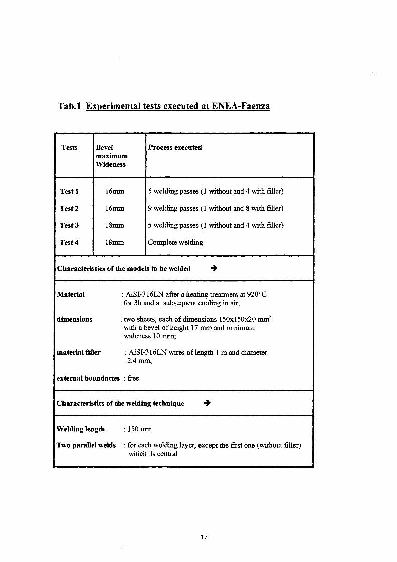
In Tab. 1 the characteristics of the experimental tests executed are reported.

The first two tests, with free external boundaries, have been performed with a reduced

number of welding passes (5 and 9, respectively) in order to acquire a knowledge of the

physical phenomena involved and to follow gradually the welding by the numerical simulation,

saving computation times.

Since from the experimental mechanical response it has been judged that the chamfer

opening was shrinking too much, the subsequent tests ( and in future also the same Coupon A)

have been performed increasing the bevel initial maximum opening, from 16 mm up to 18 mm

(see Tab. 1).

For all the 4 experimental tests reported, temperatures have been recorded by 6

thermocouples applied in 6 positions along the central line orthogonal to the welding direction

on the lower face of the sheets and sheet angular displacements have been measured after the

cooling, following each welding pass.

4. NUMERICAL TESTS

4.1 Generality

After different preliminary calculations concerning the investigations of ABAQUS code

capability of approaching the problem of interest and setting up the strategies described in

paragraph 2, considering a reduced number of passes and making reference to the

corresponding experimental tests previously presented, finally a calculation has been carried

out for the simulation of the complete welding of a sample having free boundary conditions, in

particular experimental test 4 of Tab. 1.

10

4.2 Mesh adopted

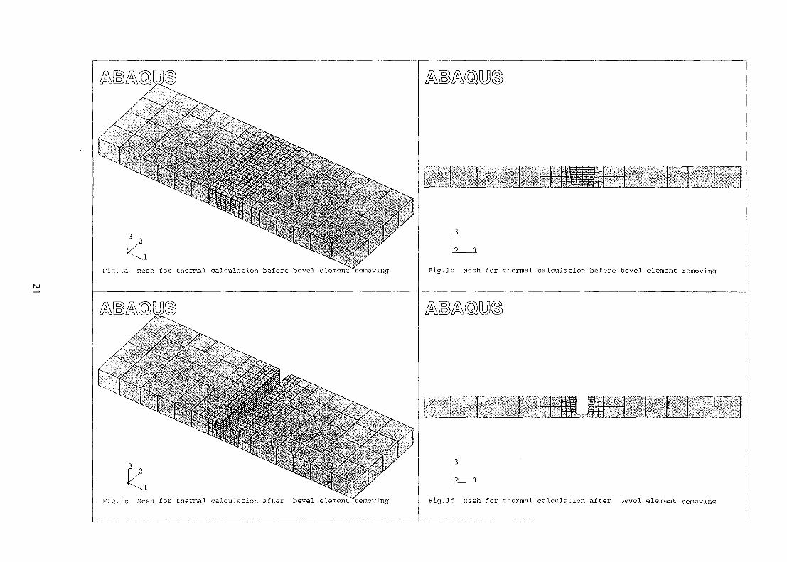
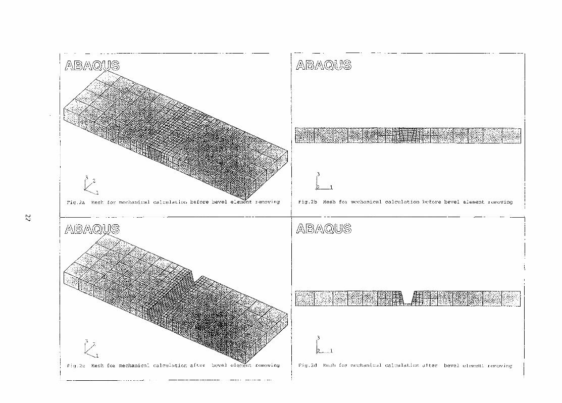
Figs. 1 and 2 show different views of the initial mesh discretization adopted in the numerical

calculation (both for the thermal part and mechanical one) in order to simulate the TIG welding

with cold filler of two sheets (as said of AISI-316LN steel), each of dimensions 150x100x20

mm3.

As can be seen, the dimension of this numerical model in the welding direction is reduced

respect to the one of the corresponding experimental sample (test 4 of Tab. 1) from 150 up to

100 mm. This was made with the aim of taking into account that the initial and final zones

welded in the real case are in a transient situation for which, often, they are not welded in a

proper way and completely.

From Fig. 1 for the thermal calculation and Fig.2 for the mechanical one it can be seen that a

fine mesh has been adopted in the zone directly interested by the weld and then a gradually

coarser mesh has been defined, proceeding far from the central welding zone. Besides, in the

thermal calculation, as said in paragraph 2, the chamfer geometry has been modified, that is,

starting from the second welding layer, the chamfer has been chosen so that it presents a

constant opening, of wideness 12 mm (see Fig.l, in particular Figs.lb and Id).

For the elements representing filler material the height has been determined on the basis of

the number of passes resulted by the corresponding experimental test. Because, in our case, the

number of passes with filler (remember that the first pass is executed without filler, see Tab. 1)

is odd, (in particular, 15) and because for each welding layer two passes are used, the last pass

has been simulated still as two parallel and contemporary passes, but with half height respect to

the previous ones.

In order to limit the number of elements to be added gradually, each pass has been

subdivided in 20 parts, constituted by only one element, having a dimension of 5 mm in the

welding direction. The dimension in the transversal direction depends on the chamfer form.

4.3 Source definition and material properties

The source movement has been simulated using the facility "AMPLITUDE by step" of

ABAQUS, applied on the elements representing the filler deposited after its introduction by

MODEL CHANGE facility for the duration time of 4 sec for each element. This time

corresponds to the time employed, on an average (remember that the welding process to be

11

simulated is carried out manually), in order to perform 5 mm of welding. Each pass is, in this

way, constituted by 40 calculation steps (20 for the introduction of each of the elements

constituting the pass examined and 20 for the source application and movement on each

element, in succession).

At the end of each pass a cooling step follows, as it occurs in the reality.

The heat source has been simulated at each pass, after the new filler-element introduction,

applying a volume source (suitably deduced by the nominal source power emitted by TIG tool,

trying to take into account the source power loss in air) on the element introduced and surface

sources (always suitably deduced by the source power above said) on the faces of all the

structure elements with which the new element is in contact.

The material physical properties have been provided by the NET team (NET team, 1998) up

to 800-1000 °C; subsequently, because not available, they have been suitably extrapolated for

the high temperatures of interest. As concerns the material mechanical properties, the necessary

stress-strain laws have been deduced and extrapolated by some experimental measures made ad

hoc (G.Bevilacqua, 1998; M.Labanti, 1998).

At the high temperatures, equal to or greater than the fusion one, in the mechanical

calculation, only the annealing effects have been taken into account by the use of an "ad hoc"

routine UMAT, as described in (Carmignani et al., 1994b). The viscoplastic material treatment

at temperatures greater than 2/3 the fusion one has been not considered in this case, because the

pieces to be welded are constituted by a strongly austenitic steel, for which the viscoplastic

effects are low and, in a first approximation (also in order to save computation times), may be

neglected.

5. RESULTS AND COMPARISONS WITH THE EXPERIENCE: ANALYSES AND

DISCUSSIONS

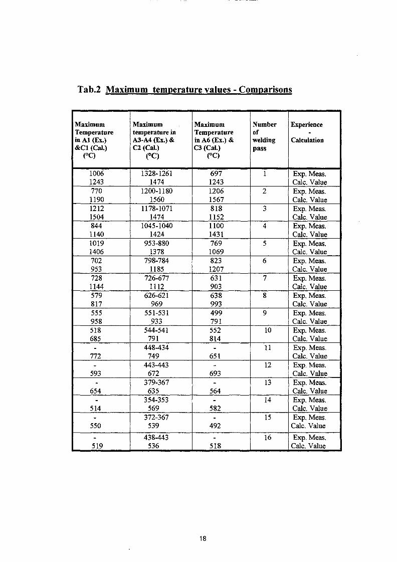
The maximum values of the temperatures measured and calculated in some positions placed

in the central zone of the lower face of pieces welded are reported in Tab.2 and the

corresponding histories of the simulation executed for the first 9 welding passes are shown in

Figs.3, 4, 5.

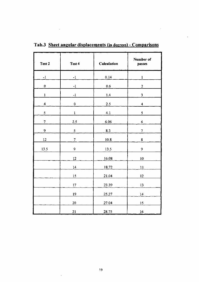
The sheet final displacement is shown in Fig. 6 and the comparison, at each welding pass,

between the angular sheet displacements calculated and the corresponding values measured for

two experimental tests (test 2 and test 4), is reported in Tab.3.

12

As concerns the maximum temperatures of Tab.2, one can see that the values calculated are,

on an average, 200-500°C higher than the corresponding ones measured. In order to evaluate

completely the means of these differences it is necessary to make some considerations:

• the experimental tests have been carried out manually; this provides differences as

concerns the duration of the welding execution and not constant values of the source

power emitted; this fact, indeed, is evident also in the spread of experimental values of

temperatures recorded;

• during the experimental tests, the temperatures at the beginning of each welding pass (in

the central zone of the lower surface) and the time duration of each pass have been

recorded, but no measure for the cooling time duration between two subsequent welding

passes has been recorded;

• in the experimental tests the beginning of the subsequent passes is conditioned by the

value of temperatures measured in the central zone of the piece lower surface and should

occur when these temperatures are nearly 100-150 °C. In the calculation, because it is not

possible to make the cooling time duration (in general, the time duration of a thermal step)

dependent on temperature value (but only on its rate), it was necessary to define a guess

for the duration of the cooling passes. Starting from a value of 6 min, the time duration has

been increased by 2 min at each subsequent pass.

It has be noted that up to the 10th pass the temperature value in the central point of the lower

surface, at the end of the cooling steps, results nearly 80-100 °C greater than the corresponding

experimental one, even if the cooling times adopted are surely greater than the ones used in the

reality; starting from the 11* pass, on the contrary, the final temperatures after each cooling

step result lower than the corresponding experimental values recorded.

This situation, jointly with the fact that the maximum temperatures are too high, seems to

single out three possible causes:

• to have adopted a too high value for the source power;

• to have underestimated the thermal exchange with the environment;

• to have extrapolated, in an uncorrected way, the material physical properties at the

temperatures greater than 800-1000 °C.

Indeed, analyzing the temperature behaviour in some points, it can be noted that the

maximum values near to 1800 °C are reached; besides, the radiation effects (in order to reduce

the computation times) have been completely neglected. However, these two facts do not seem

sufficient to explain the systematic differences, of nearly 400 °C between the maximum

13

temperature values calculated and measured; at the most, they can explain the highest

temperatures calculated at the end of each cooling step.

The uncorrected extrapolation of the material specific heat and thermal conductivity at

temperatures higher than 800-1000 °C (as said, not available) can, on the contrary, explain the

too high maximum temperatures calculated. Different hypotheses for these values have been

taken into account and new calculations are, now, in course.

As concerns the sheet angular displacement, whose value results at the end of the process

greater than 30% compared with the experimental corresponding one, it is necessary to observe

that the experimental values for this quantity present a very great spread and the experimental

test of reference for the final value (that is, test 4) presented an initial configuration having

already an angular deformation of nearly -1 degree. Besides, considering that (seeTab.3) at the

end of the 9th pass the angular displacement value of this test is 4 degrees lower than the

corresponding value of the test 2 (see always Tab.3), one can reasonably think that the

difference, between calculation and experience, is really much lower than 30%; besides, it will

probably decrease if the thermal source is defined lower.

6. CONCLUSIONS

From the comparisons made, it is clear that further studies and improvements seem still be

necessary in order to consider sufficiently accurate the numerical simulation of the TIG

welding process here presented. Indeed, sensitive analyses are in course in order to understand

the causes of the differences between the maximum temperature values calculated and

measured and the influence of these on the angular sheet displacements. However, it seems

that it can be said that:

• the TIG welding technique can be simulated utilizing AB AQUS/S code;

• an initial computation strategy has been found and tested; the use of this strategy has

allowed promising results to be obtained;

• even if the strategy followed is heavy, both for the input data preparation, for the

computation times and space-disk required (in particular, in ABAQUS versions adopted,

5.7 and 5.8, which do not use VTEWER modulus) , it seems possible, adopting this same

strategy, to approach the simulation of Coupons A, for which more accurate and more

extended experimental measures (also strain and residual stress measures) are available.

14

7. REFERENCES

B.Carmignani, A.Daneri, S.Giambuzzi, G.Toselli: "Thermal and Mechanical Response of Steel

Sheet Welded by Laser Process: Pre-analysis Made by ABAQUS/S Code", ENEA

RT/INN/94/45,1994.

B.Carmignani, A.Daneri, G.Toselli, R.Vitali, G.L.Zanotelli, M.Bellei: "Evaluation of the Sheet

Mechanical Response to Laser Welding Processes".^ ABAQUS Users' Conference

Proceedings - Paris (France), 31May-2 June 1995 and ENEA-RT/INN/95/11,1994.

B.Carmignani, R.Mares, G.Toselli: "User Routine UMATDevelopment and Use in order to

Treat the MetalElastoviscoplastic Behaviour at High Temperatures". 11th ABAQUS Users'

Conference Proceedings - Newport (R.I. - USA), 27-29 May, 1998.

B.Carmignani, RMares, G.Toselli: "Transient Finite Element Analysis of Deep Penetration

Laser Welding Process in a Single Pass Butt-Welded Thick Steel Plate", (to be published on

the journal "COMP. METH. in APP. MECH. and ENG.", 1999.)

B.S.Tranchina, A.Mancorti, T.Minghetti, G.Panzani, D.Trestini: "Report on experimental tests

for TIG welding technique with filler carried out atENEA, Faenza (Italy)", to be published,

1999.

NET team: private communication, (Garching, Germany), 1998.

G.Bevilacqua private communication, (NET team-Garching, Germany), 1998.

MXabanti, B.S.Tranchina: private communication, (ENEA-Faenza, Italy), 1998.

15

Tab.l Experimental tests executed at ENEA-Faenza

Tests BevelmaximumWideness

Process executed

Testl

Test 2

Test 3

Test 4

16mm

16mm

18mm

18mm

5 welding passes (1 without and 4 with filler)

9 welding passes (1 without and 8 with filler)

5 welding passes (1 without and 4 with filler)

Complete welding

Characteristics of the models to be welded

Material : AISI-316LN after a heating treatment at 920°Cfor 3h and a subsequent cooling in air;

dimensions : two sheets, each of dimensions 150x150x20 mm3

with a bevel of height 17 mm and minimumwideness 10 mm;

material filler : AISI-316LN wires of length 1 m and diameter2.4 mm;

external boundaries : free.

Characteristics of the welding technique

Welding length : 150 mm

Two parallel welds : for each welding layer, except the first one (without filler)which is central

17

Tab.2 Maximum temperature values - Comparisons

MaximumTemperaturein Al (Ex.)&C1 (Cal.)

(°C)

100612437701190121215048441140101914067029537281144579817555958518685

772

593

654

514

550

519

Maximumtemperature inA3-A4 (Ex.) &C2 (Cal.)

(°Q

1328-12611474

1200-11801560

1178-10711474

1045-10401424

953-8801378

798-7841185

726-6771112

626-621969

551-531933

544-541791

448-434749

443-443672

379-367635

354-353569

372-367539

438-443536

MaximumTemperaturein A6 (Ex.) &C3 (Cal.)

(°Q

69712431206156781811521100143176910698231207631903638993499791552814

651

693

564

582

492

518

Numberofweldingpass

1

2

3

4

5

6

7

8

9

10

11

12

13

14

15

16

Experience

Calculation

Exp. Meas.Calc. ValueExp. Meas.Calc. ValueExp. Meas.Calc. ValueExp. Meas.Calc. ValueExp. Meas.Calc. ValueExp. Meas.Calc. ValueExp. Meas.Calc. ValueExp. Meas.Calc. ValueExp. Meas.Calc. ValueExp. Meas.Calc. ValueExp. Meas.Calc. ValueExp. Meas.Calc. ValueExp. Meas.Calc. ValueExp. Meas.Calc. ValueExp. Meas.

Calc. Value

Exp. Meas.Calc. Value

18

Tab.3 Sheet angular displacements (in degrees) - Comparisons

Test 2

-1

0

1

4

5

7

9

12

13.5

Test 4

-1

-1

-1

0

1

2.5

5

7

9

12

14

15

17

19

20

21

Calculation

0.14

0.6

1.4

2.5

4.1

6.06

8.3

10.8

13.5

16.08

18.72

21.04

23.39

25.27

27.04

28.75

Number ofpasses

1

2

3

4

5

6

7

8

L 9

10

11

12

13

14

15

16

19

1

Fig. la Mesh for thermal calculation before bevel elementT"*removirig Fig.lb Mesh for thermal calculation before bevel element removing

.1

Fig.lc Mesh for thermal calculation after bevel element lemoving Fig.Id Mesh for thermal calculation after bevel element removing

1

Fig.2a Mesh for mechanical calculation before bevel element removing Fig.2b Mesh for mechanical calculation before bevel element removing

3 „

Fig.2c Mesh for mechanical calculation after bevel element removing Fig.2d Mesh for mechanical calculation after bevel element removing

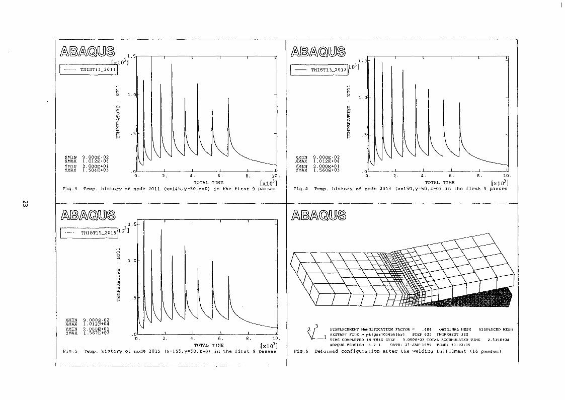
XMIN 9.000E-02XMAX 1.012E+04YMIN 2.000E+01YMAX 1.504E+03 0. 4. 6. 8. 10.

TOTAL TIME [xlO3]Fig.3 Temp, history of node 2011 (x=145,y=50,z=0) in the first 9 passes

UJ

XMIN 9.000E-02XMAX 1.012E+04YMIN 2.000E+01YMAX 1.560E+03 2. 8. 10.4. 6.

TOTAL TIME [xlO3]Fig.4 Temp, history of node 2013 (x=150,y=50,z=0) in the first 9 passes

XMINXMAXYMINYMAX

rig . ci

9 .000E-021 .012E+042 .OOOE+011.567E+03

2. 4. 6TOTAL TIME

Temp, history of node 2015 (x=155,y=50,z=0) in the first

8. 10.

[xlO3]9 passes

DISPLACEMENT MAGNIFICATION FACTOR = .484 ORIGINAL MESH DISPLACED MESHRESTART FILE = ptic)3rl016pk£brl STEP 623 INCREMENT 322TIME COMPLETED IN THIS STEP 3.0OOE*O3 TOTAL ACCUMULATED TIME 2.515E+O1ABAOUS VERSION: 5.7-1 DATE: 27-JAN-1999 TIME: 11:02:19

Fig.6 Deformed configuration after the welding fulfilment (16 passes)

Unita Comunicazione e InformazioneLungotevere Grande Ammiraglio Thaon di Revel, 76 - 00196 Roma

Sito Web http://www.enea.it

Stampa Centro Stampa Tecnografico - C.R. Frascati

Finito di stampare nel mese di novembre 1999

24