M a t h e m a t i c aB a l k a n i c a

—————————

NewSeries Vol. 20, 2006, Fasc. 3-4

Numerical Solution of Monge-Ampere Equation

M. Bouchiba and F. Ben Belgacem

Presented by V. Kiryakova

We show that the numerical solution, of the fully non linear Monge-Ampre equation in

two dimension, can be obtained by resolving an optimisation problem implying the resolution

of a quasilinear Dirichlet problem. A gradient method is used. We give a no classical method

to compute the gradient.

Key Words Monge-Ampre, finite elements, gradient method.

1. Introduction

In this paper we give a numerical solution of the following Monge-Ampreproblem :

(PI)

det[D2u] = f2(x, u) x ∈ Ωu|Γ = 0, u convex on Ω.

Where Ω is a smooth convex and bounded domain in R2, [D2u] is the Hessian

of u and f ∈ C2(Ω × R), f > 0 on Ω × R , and∂f

∂s(x, s) ≥ 0.

The problem (PI) has a unique strictly convex solution uI ∈ C2(Ω)∩W 1,∞(Ω)(see[1] ).

We propose a variationnal method for the approximation of the solutionuI of (PI) as in [2]. We show that (PI) is equivalent to the following problem :

(PII)ming∈V

J(g),

with

J(g) =1

2

∫

Ω[det[D2u(g)] − f 2(x, u(g))]2dx

370 M. Bouchiba, F. Belgacem

where u(g) is solution of the Dirichlet problem

Pg

−∆u + 2f(., u) = −gu|Γ = 0

and we show that uI = u(g), where g = Arg(minJ(g))

In section 2 we prove the equivalence between (PI) and (PII) and we usea Galerkin-finite elements to approximize the solution u(g) of (Pg). In section3 we give a non classical method to compute the gradient of the functional J .In the end we give a numerical test.

2. An equivalent problem

Let us consider the following assumptions

• (H1) f ∈ C2(Ω × R) ∩ W 2,∞(Ω × R).

• (H2) f(x, s) ≥ α0 > 0, ∀s ∈ R−, ∀x ∈ Ω.

• (H3)∂f

∂s(x, s) > 0, ∀s ∈ R−, ∀x ∈ Ω.

• (H4) s 7−→ f(., s) is convex ∀s ∈ R−.

2.1. The Problem (PII)

Let λ1 and λ2 be the eigenvalues of the matrix [D2u]. We have

λ1 + λ2 = ∆uI ,λ1λ2 = f(., uI).

Then λ1 and λ2 are the solutions of

X2 − ∆uIX + f2(., uI) = 0.

So

(∆uI)2 − 4f2(., uI) ≥ 0.

Since uI is convex and f > 0 we should have

∆uI − 2f ≥ 0.

If we put

g = ∆uI − 2f,(2.1)

Numerical Solution of Monge-Ampere Equation 371

it is clear that uI is solution of the following problem

Pg

−∆u + 2f(., u) = −gu|Γ = 0

(2.2)

To compute g, we consider the functional

J(g) =1

2

∫

Ω[det[D2u(g)] − f 2(x, u(g))]2dx(2.3)

where u(g) is the solution of the Dirichlet problem

(Pg)

−∆u + 2f(., u) = −gu|Γ = 0.

(2.4)

We remark that J is well-defined if u(g) ∈ W 2,4(Ω) and f 2(., u(g)) ∈ L2(Ω).We recall the following result:

Theorem 2.1. Under assumptions (H3) and g ∈ L2(Ω) the quasilinear

elliptic problem (Pg) has a unique solution u(g) ∈ H10 (Ω). (see[4]).

We have the following result:

Theorem 2.2. Problems (PI) and (PII). are equivalents

P r o o f. By (2.2) we have uI = u(g) so J(g) = 0.Let g a solution of (PII) then J(g) = 0 so

det[D2u(g)] = f,

u(g)|Γ = 0.

Since ∆u(g) = 2f + g > 0 and det[D2u(g) > 0 we have u(g) is strictly convexand from the uniqueness of solution for (PI) we get u(g) = uI .

Re ma r k 2.3 From the previous section we can deduce that the com-putation by finite elements method of uI is possible by resolving (P

g) if one hasg for this purpose we resolve (PII).

3. The numerical resolution of (PII)

To numerical resolve (PII) we start linearizing (Pg) by considering asequence of linear problems which are resolved by finite elements method. Tocompute g we use a gradient method.

3.1. Resolution of the problem (Pg)3.1.1. Linearisation of the problem (Pg) We assume that

g ∈ H1+(Ω) = v ∈ H1(Ω)/v ≥ 0

372 M. Bouchiba, F. Belgacem

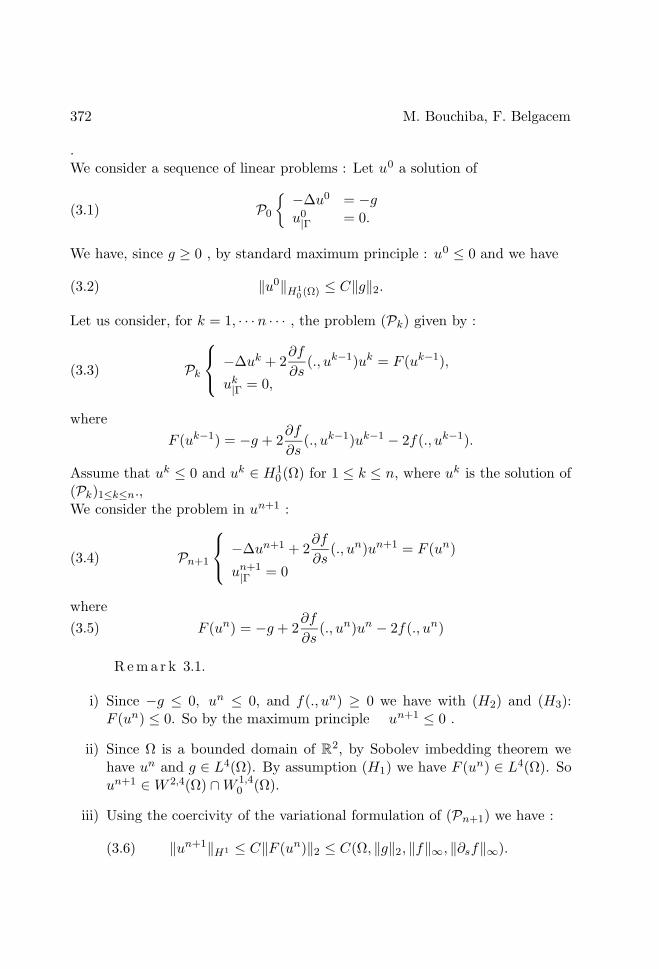
.We consider a sequence of linear problems : Let u0 a solution of

P0

−∆u0 = −gu0|Γ = 0.

(3.1)

We have, since g ≥ 0 , by standard maximum principle : u0 ≤ 0 and we have

‖u0‖H1

0(Ω) ≤ C‖g‖2.(3.2)

Let us consider, for k = 1, · · · n · · · , the problem (Pk) given by :

Pk

−∆uk + 2∂f

∂s(., uk−1)uk = F (uk−1),

uk|Γ = 0,

(3.3)

where

F (uk−1) = −g + 2∂f

∂s(., uk−1)uk−1 − 2f(., uk−1).

Assume that uk ≤ 0 and uk ∈ H10 (Ω) for 1 ≤ k ≤ n, where uk is the solution of

(Pk)1≤k≤n.,We consider the problem in un+1 :

Pn+1

−∆un+1 + 2∂f

∂s(., un)un+1 = F (un)

un+1|Γ = 0

(3.4)

where

F (un) = −g + 2∂f

∂s(., un)un − 2f(., un)(3.5)

R e ma r k 3.1.

i) Since −g ≤ 0, un ≤ 0, and f(., un) ≥ 0 we have with (H2) and (H3):F (un) ≤ 0. So by the maximum principle un+1 ≤ 0 .

ii) Since Ω is a bounded domain of R2, by Sobolev imbedding theorem we

have un and g ∈ L4(Ω). By assumption (H1) we have F (un) ∈ L4(Ω). Soun+1 ∈ W 2,4(Ω) ∩ W 1,4

0 (Ω).

iii) Using the coercivity of the variational formulation of (Pn+1) we have :

‖un+1‖H1 ≤ C‖F (un)‖2 ≤ C(Ω, ‖g‖2, ‖f‖∞, ‖∂sf‖∞).(3.6)

Numerical Solution of Monge-Ampere Equation 373

.

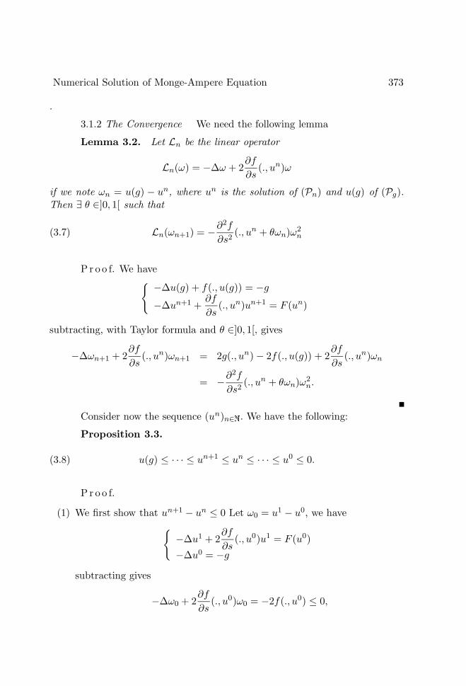
3.1.2 The Convergence We need the following lemma

Lemma 3.2. Let Ln be the linear operator

Ln(ω) = −∆ω + 2∂f

∂s(., un)ω

if we note ωn = u(g) − un, where un is the solution of (Pn) and u(g) of (Pg).Then ∃ θ ∈]0, 1[ such that

Ln(ωn+1) = −∂2f

∂s2(., un + θωn)ω2

n(3.7)

P r o o f. We have

−∆u(g) + f(., u(g)) = −g

−∆un+1 +∂f

∂s(., un)un+1 = F (un)

subtracting, with Taylor formula and θ ∈]0, 1[, gives

−∆ωn+1 + 2∂f

∂s(., un)ωn+1 = 2g(., un) − 2f(., u(g)) + 2

∂f

∂s(., un)ωn

= −∂2f

∂s2(., un + θωn)ω2

n.

Consider now the sequence (un)n∈ . We have the following:

Proposition 3.3.

u(g) ≤ · · · ≤ un+1 ≤ un ≤ · · · ≤ u0 ≤ 0.(3.8)

P r o o f.

(1) We first show that un+1 − un ≤ 0 Let ω0 = u1 − u0, we have

−∆u1 + 2

∂f

∂s(., u0)u1 = F (u0)

−∆u0 = −g

subtracting gives

−∆ω0 + 2∂f

∂s(., u0)ω0 = −2f(., u0) ≤ 0,

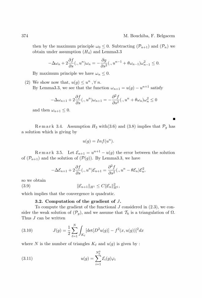
374 M. Bouchiba, F. Belgacem

then by the maximum principle ω0 ≤ 0. Subtracting (Pn+1) and (Pn) weobtain under assumption (H4) and Lemma3.3

−∆ωn + 2∂f

∂s(., un)ωn = −

∂g

∂s2(., un−1 + θωn−1)ω

2n−1 ≤ 0.

By maximum principle we have ωn ≤ 0.

(2) We show now that, u(g) ≤ un ,∀ n.By Lemma3.3, we see that the function ωn+1 = u(g) − un+1 satisfy

−∆ωn+1 + 2∂f

∂s(., un)ωn+1 = −

∂2f

∂s2(., un + θωn)ω2

n ≤ 0

and then ωn+1 ≤ 0.

R e ma r k 3.4. Assumption H3 with(3.6) and (3.8) implies that Pg hasa solution which is giving by

u(g) = Inf(un).

Re ma r k 3.5. Let En+1 = un+1 − u(g) the error between the solutionof (Pn+1) and the solution of (P(g)). By Lemma3.3, we have

−∆En+1 + 2∂f

∂s(., un)En+1 =

∂2f

∂s2(., un − θEn)E2

n,

so we obtain‖En+1‖H1 ≤ C‖En‖

2H1 ,(3.9)

which implies that the convergence is quadratic.

3.2. Computation of the gradient of J .

To compute the gradient of the functional J considered in (2.3), we con-sider the weak solution of (Pg), and we assume that Th is a triangulation of Ω.Thus J can be written

J(g) =1

2

N∑

`=1

∫

K`

[det[D2u(g)] − f 2(x, u(g))]2dx(3.10)

where N is the number of triangles K` and u(g) is given by :

u(g) =

N0

h∑

i=1

Ei(g)ϕi(3.11)

Numerical Solution of Monge-Ampere Equation 375

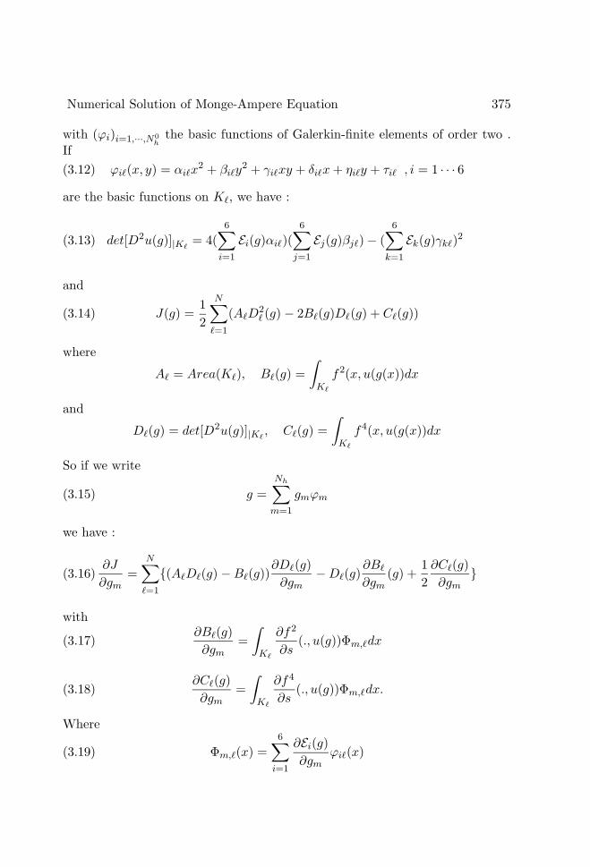
with (ϕi)i=1,···,N0

h

the basic functions of Galerkin-finite elements of order two .If

ϕi`(x, y) = αi`x2 + βi`y

2 + γi`xy + δi`x + ηi`y + τi` , i = 1 · · · 6(3.12)

are the basic functions on K`, we have :

det[D2u(g)]|K`= 4(

6∑

i=1

Ei(g)αi`)(6∑

j=1

Ej(g)βj`) − (6∑

k=1

Ek(g)γk`)2(3.13)

and

J(g) =1

2

N∑

`=1

(A`D2` (g) − 2B`(g)D`(g) + C`(g))(3.14)

where

A` = Area(K`), B`(g) =

∫

K`

f2(x, u(g(x))dx

and

D`(g) = det[D2u(g)]|K`, C`(g) =

∫

K`

f4(x, u(g(x))dx

So if we write

g =

Nh∑

m=1

gmϕm(3.15)

we have :

∂J

∂gm

=

N∑

`=1

(A`D`(g) − B`(g))∂D`(g)

∂gm

− D`(g)∂B`

∂gm

(g) +1

2

∂C`(g)

∂gm

(3.16)

with∂B`(g)

∂gm

=

∫

K`

∂f2

∂s(., u(g))Φm,`dx(3.17)

∂C`(g)

∂gm

=

∫

K`

∂f4

∂s(., u(g))Φm,`dx.(3.18)

Where

Φm,`(x) =

6∑

i=1

∂Ei(g)

∂gm

ϕi`(x)(3.19)

376 M. Bouchiba, F. Belgacem

and

∂D`(g)

∂gm

= 4

(6∑

i=1

∂Ei(g)

∂gm

αi`

)( 6∑

j=1

Ej(g)βj`

)

+ 4( 6∑

i=1

Ei(g)αi`

)( 6∑

j=1

∂Ej(g)

∂gm

βj`

)

− 2( 6∑

k=1

Ek(g)γk`

)( 6∑

k=1

∂Ek(g)

∂gm

γk`

)

(3.20)

So to compute the gradient of J we need

∂Ei(g)

∂gm

i = 1, · · · , N 0h , m = 1, · · · , Nh(3.21)

We consider then equation (2.4) and after partial derivation we have by(3.15)

−∆ωm + 2∂f

∂s(., u(g))ωm = −ϕm,

ωm|Γ = 0.(3.22)

Where ωm =∂u(g)

∂gm

. Note too using (3.11) that

∂u(g)

∂gm

=

N0

h∑

i=1

∂Ei(g)

∂gm

ϕi

and (3.22) give

ωm =

N0

h∑

i=1

ηmi ϕi.(3.23)

So resolving (3.22) by the use of the finite elements method we obtain with(3.23)

∂Ei(g)

∂gm

= ηmi i = 1, · · · , N 0

h m = 1, · · · , Nh.(3.24)

4. Numerical test

In order to test this method, we have shosen, an example of problem(PI) which we know its explicet solution. The latter is shosen in order to becompared to the computed solution.

Numerical Solution of Monge-Ampere Equation 377

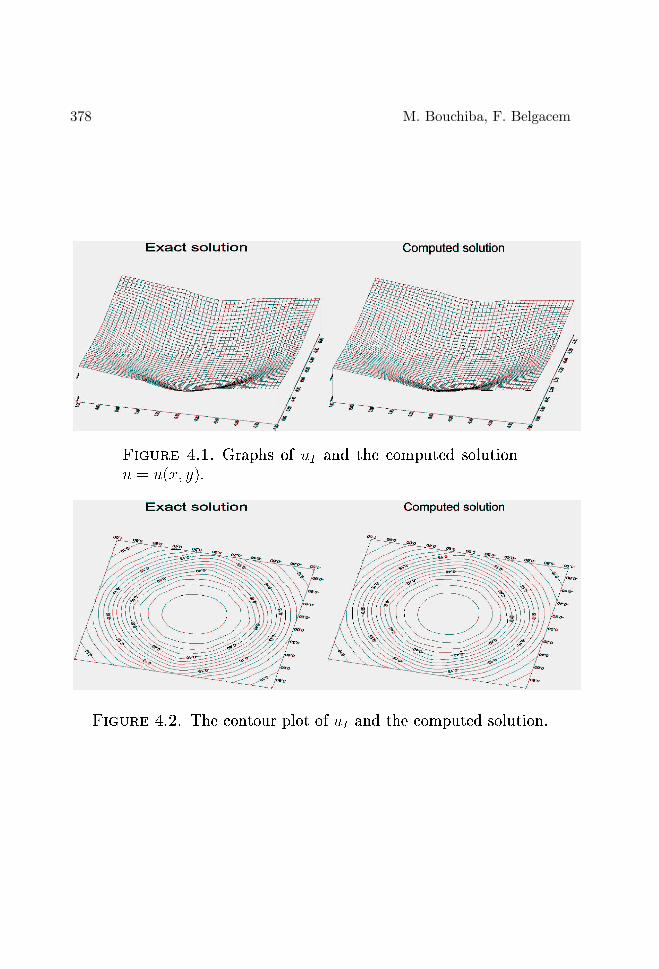
Ex a mp l e Example 4.1. We take Ω the unit disque and

f((x, y), u) = 4 (3 + 2Log (1 + u)) (1 + u)2 .

It’s clear that f verifies all assuptions (H1), (H2, ) (H3) and (H4). The solutionof (PI) is the following

uI(x, y) = e(x2+y2−1) − 1.

In Fig. 4.1 and Fig. 4.2 we present the computed solution obtained by applyingthis method at 10 iterations compared to the exact solution uI .

References

[1] P . L . L i o n s. Sur les quations de Monge-Ampere I, Manscripta. Math.,41, 1983.

[2] F . B e n B e l g a c em. Computation method for the Monge-Ampre equa-tion, IJAM, 16, 2005,(preprint).

[3] D . G i l b a r g , N . S . T ru d i n g e r. Elliptic Partial Differential Equations

of Second Order, Spring-Verlag, Heidelberg (1983)

[4] O . K a v i a n . Intoduction a la thorie des points critiques, Springer-Verlag(1991)

Department of Mathematics Received 02.04.2005

Faculty of Sciences of Tunis,

1060 Tunis, Tunisia

378 M. Bouchiba, F. Belgacem