Embed Size (px)
Citation preview
Numerical Solution for the Variable Order Fractional Partial Differential Equation with Bernstein polynomials
1 Jinsheng Wang, 2 Liqing Liu, 3 Lechun Liu, 4 Yiming Chen
1, First AuthorYanshan University, [email protected] *2,Corresponding AuthorYanshan University, [email protected]
3,4Yanshan University, [email protected], chenym.ysu.edu.cn
Abstract In this paper, we develop a framework to obtain numerical solution of the variable order fractional
partial differential equation using Bernstein polynomials. The main characteristic behind this approach is that we derive a fractional order operational matrix of Bernstein polynomials. With the operational matrix, the equation is transformed into the products of several dependent matrixes which can also be regarded as the system of linear equations after dispersing the variable. By solving the linear system of algebraic equations, the numerical solutions are acquired. Only a small number of Bernstein polynomials are needed to obtain a satisfactory result. Numerical examples are provided to show that the method is computationally efficient.
Keywords: Bernstein polynomials, the variable order fractional partial differential equation,
Numerical solution,the absolute error
1. Introduction
In recent years, fractional calculus has attracted many researchers successfully in different disciplines of science and engineering. One of the main advantages of the fractional calculus is that the fractional derivatives provide a superior approach for the description of memory and hereditary properties of various materials and processes [1]. Many numerical methods using different kinds of fractional derivative operators for solving different types of fractional differential equations have been proposed. The most commonly used ones are Adomian decomposition method (ADM) [2][3], Variational iteration method (VIM) [4], generalized differential transform method (GDTM) [5-7], generalized block pulse operational matrix method [8] and wavelet method [9][10] and other methods [11-13].
Recently, more and more researchers are finding that numerous important dynamical problems exhibit fractional order behavior which may vary with space and time. This fact illustrates that variable order calculus provides an effective mathematical framework for the description of complex dynamical problems. The concept of a variable order operator is a much more recent development, which is a new orientation in science. Different authors have proposed different definitions of variable order differential operators, each of these with a specific meaning to suit desired goals. The variable order operator definitions recently proposed in the science include the Riemann-Liouvile definition, Caputo definition, Marchaud definition, Coimbra definition and Grünwald definition [14-18].
Since the kernel of the variable order operators is too complex for having a variable-exponent, the numerical solutions of variable order fractional differential equations are quite difficult to obtain, and have not attracted much attention. Therefore, the development of numerical techniques to solve variable order fractional differential equations has not taken off. To the best of the authors’ knowledge, there are few references arisen on the discussion of variable order fractional differential equation. In several emerging, most authors adopt difference method to deduce an approximate scheme. For example, Coimbra [16] employed a consistent approximation with first-order accurate for the solution of variable order differential equations. Soon et al. [19] proposed a second-order Runge–Kutta method which is consisting of an explicit Euler predictor step followed by an implicit Euler corrector step to numerically integrate the variable order differential equation. Lin et al. [20] studied the stability and the convergence of an explicit finite-difference approximation for the variable-order fractional diffusion equation with a nonlinear source term. Zhuang et al. [21] obtained explicit and implicit Euler approximations for the fractional advection–diffusion nonlinear equation of variable-order. Aiming a variable-order anomalous subdiffusion equation, Chen et al. [22] employed two numerical schemes one
Numerical Solution for the Variable Order Fractional Partial Differential Equation with Bernstein polynomials Jinsheng Wang, Liqing Liu, Lechun Liu, Yiming Chen
International Journal of Advancements in Computing Technology(IJACT) Volume 6, Number 3, May 2014
22
fourth order spatial accuracy and with first order temporal accuracy, the other with fourth order spatial accuracy and second order temporal accuracy. However, as far as we know, no one had attempted to seek the numerical solution of the variable order fractional equations.
So in this paper, we introduce the Bernstein polynomials to seek the numerical solution of the variable order fractional partial equation. With the simple structure and perfect properties [23][24], the Bernstein polynomials play an important role in various areas of mathematics and engineering. Those polynomials have been widely used in the solution of integral equations and differential equations [23-29].
In this paper, our study focuses on a class of fractional partial differential equation as follows:
, ,
, ,x t
x t
u x t u x tf x t
x t
(1)
Subject to the initial conditions
,0
0,
u x g x
u t h t
(2)
where , /x xu x t x and
, /t tu x t t are fractional derivative of Caputo sense,
,f x t is the known continuous function, ,u x t is the unknown function, 0 , 1x t .
The reminder of the paper is organized as follows: Sections 2 and 3 are preparative, the definitions and properties of the variable order fractional order integrals and derivatives and Bernstein polynomials are given in Sections 2 and 3. In Section 4, the fractional operational matrixes of Bernstein polynomials are derived and we applied the operational matrix to solve the equation as given at beginning. In Section 5, we present some numerical examples to illustrative the method and to demonstrate efficiency of the method. We end the paper with a few concluding remarks in Section 6.
2. Basic definitions and properties of the variable order fractional integrals and derivatives
Form the definitions and properties of fractional order calculus, we can derive the definitions and properties of the variable order fractional order calculus [14-16].
i) Riemann-Liouville fractional integral of the first kind with order t
11
, 0 Re 0ttt
a aI u t t T u T dT t t
t
(3)
ii) Riemann-Liouville fractional derivate of the first kind with order t
1
11
mtt
a m t ma
udD u t d m t m
dtm t t
(4)
but t t
a aD I u u .
iii) Captuo’s fractional derivate with order t
0
0 01
1 1
tttt u u t
D u t t u dt t
(5)
where 0 1t . If we assume the starting time in a perfect situation, we can get the definition as
follows:
Numerical Solution for the Variable Order Fractional Partial Differential Equation with Bernstein polynomials Jinsheng Wang, Liqing Liu, Lechun Liu, Yiming Chen
23
0
10 1
1
tttD u t t u d tt
(6)
with the definition above, we can get the following formula 0 1t :
0 0
11,2,3
1
ta tD x
xt
(7)
3. Bernstein Polynomials and their properties
3.1. The definition of Bernstein Polynomials basis The Bernstein Polynomials of degree n are defined by
, 1n ii
i n
nB x x x
i
(8)
By using the binomial expansion of 1n i
x , Eq. (9) can be expressed as:
,0
1 1kn i
n ii i ki n
k
n n n iB x x x x
i i k
(9)
Now, we define:
T
0, 1, ,, , ,n n n nx B x B x B x Φ (10)
where we can have
nx xΦ AT (11)
where
0 1 0
0 1
0
0 01 1 1
0 0 1 0 0
1 10 1 1
1 0 1 1
0 0 1
n
n
n n n n n
n
n n n n
n
n
n
A (12)
T21, , , , nn x x x x T (13)
Clearly
1n x xT A Φ (14)
3.2. function approximation
A function 2 0,1f x L can be expressed in terms of the Bernstein Polynomials basis. In
practice, only the first 1n terms of Bernstein Polynomials are considered. Hence
Numerical Solution for the Variable Order Fractional Partial Differential Equation with Bernstein polynomials Jinsheng Wang, Liqing Liu, Lechun Liu, Yiming Chen
24

,0
nT
i i ni
f x c B x c x
Φ (15)
where 0 1, , ,T
nc c c c .
Then we have
1 ,f xc Q Φ (16)
where Q is an 1 1n n matrix, which is called the dual matrix of xΦ .
1
0
1
0
1
0
T
T
n n
T Tn n
T
x x dx
x x dx
x x dx
Q Φ Φ
AT AT
A T T A
AHA
(17)
where H is a Hilbert matrix:
1 11
2 11 1 1
2 3 2
1 1 1
1 2 2 1
n
n
n n n
H (18)
We can also approximate the function 2, 0,1 0,1u x t L as following:
, , ,0 0
,n n
Ti j i n j n
i j
u x t u B x B t x t
Φ UΦ (19)
where
00 01 0
10 11 1
0 1
n
n
n n nn
u u u
u u u
u u u
U (20)
AndU can be obtained as following:
1 1, , ,x t u x t U Q Q (21)
3.3. Convergence analysis
Suppose that the function : 0,1f is 1m times continuously differentiable,
1 0,1mf C , and 0, 1, 2, ,{ , , , }n n n n nSpan B B B B Y .If T xc Φ is the best approximation of
f out ofY , then the mean error bound is presented as follows:
Numerical Solution for the Variable Order Fractional Partial Differential Equation with Bernstein polynomials Jinsheng Wang, Liqing Liu, Lechun Liu, Yiming Chen
25
2 3
2
2
2
1 ! 2 3
m
T MSf
m m
c Φ (22)
where 1[0,1] 0 0max , max 1 ,m
xM f x S x x .
Proof: We consider the Taylor polynomials
2
0 01 0 0 0 0 02 !
m
mx x x xf x f x f x x x f x f x
m
which we know
1
1 01 0,1
1 !
m
m x xf x f x f
m
since T xc Φ is the best approximation of f , so we have
212 2
1 122 0
211 1 0
0
2 1 2 2
02 0
2 2 3
2
1 !
1 !
2
1 ! 2 3
T
m
m
m
m
f f f f x f x dx
x xf dx
m
Mx x dx
m
M S
m m
c Φ
And taking square roots we have the above bound. 4. Proposed method for the numerical solution of the fractional partial differential equation
Now, consider Eq. (1). If we approximate the function ,u x t with the Bernstein Polynomials, it
can be written as Eq. (19).Then we have
,x Tx
x x
Tx
x
x tu x t
x x
xt
x
Φ UΦ
ΦUΦ
Numerical Solution for the Variable Order Fractional Partial Differential Equation with Bernstein polynomials Jinsheng Wang, Liqing Liu, Lechun Liu, Yiming Chen
26
1
2
1
2 10
2 1
0 0 01
20 0
2
10 0
1
Txn T
x
x n x T
T
x
T
xn
TT T
xt
x
nx x t
x n x
xxx
tx
nx x
n x
x t
TA UΦ
A UΦ
A UΦ
Φ A MA UΦ
(23) Also we have
1
1
,
2 10
2 1
0 0 0
20 0
2
10 0
1
t Tt
t t
tT
t
tnT
t
T
t n tT
t
Tn
t
T
x tu x t
t t
tx
t
tx
t
nx t t
t n t
tt
x t
nt
n t
x t
Φ UΦ
ΦΦ U
TΦ UA
Φ UA
Φ UA T
Φ UANA Φ
(24)
Numerical Solution for the Variable Order Fractional Partial Differential Equation with Bernstein polynomials Jinsheng Wang, Liqing Liu, Lechun Liu, Yiming Chen
27
Now we define
0 0 0
20 0
2
10 0
1
x
x
xx
nx
n x
M (25)
we define
0 0 0
20 0
2
10 0
1
t
t
tt
nt
n t
N (26)
M , N are called the fractional order operational matrix of Bernstein polynomials. Substituting Eq. (23), Eq. (24) into Eq. (1), we have
1 1 ,TT T Tx t x t f x t Φ A MA UΦ Φ UANA Φ (27)
Dispersing Eq. (27) by the points , 1, 2, , ; 1,2, ,i j x tx t i n j n , by using Mathematica
software, we can obtainU which is unknown. At last, we can obtain the numerical solution as
,u x t x tΦ UΦ .
5. numerical examples
To demonstrate the efficiency and the practicability of the proposed method based on Bernstein polynomials method, we present some examples and find their solution via the method described in the previous section.
Example 1:
sin 1 /3 cos 1 /3
sin 1 /3 cos 1 /3
2
, ,,
,0 10 1
0, 0 , 0,1 0,1
x t
x t
u x t u x tf x t
x t
u x x x
u t x t
where
2 cos 5 sin223 3 3 3
2
60 1 5 3 cos 180 1 8 9 +sin
2 1 2 110 7cos cos cos sin 8 sin 5 sin 2 sin
3 3 3 3
t x
t x x t t t x x xf
t t t x x x x
Numerical Solution for the Variable Order Fractional Partial Differential Equation with Bernstein polynomials Jinsheng Wang, Liqing Liu, Lechun Liu, Yiming Chen
28
The exact solution of the above equation is 22, 10 1 1u x t x x t .
We solved the problem by adopting of the technique described in section 4 and by making use of
Mathematica 9.0.
Taking 3n , dispersing 1 1, 1,2,3; 1,2,3
3 6 3 6ji
i j i j
kkx t k k , we can obtain the
matrixU as follows:
0 0 0 0
0 0 0 0
10 50 80 40
3 9 9 30 0 0 0
U
The numerical solution is ,u x t x tΦ UΦ , as the matrix U is given above, and
3 2 3 22 3 2 31 3 1 3 1 , 1 3 1 3 1T T
x x x x x x x t t t t t t t Φ Φ
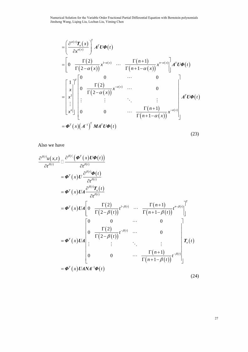
The absolute error between the exact solution and the numerical solution is displayed as follows:
Figure 1. The absolute error for Example 1 of 3n
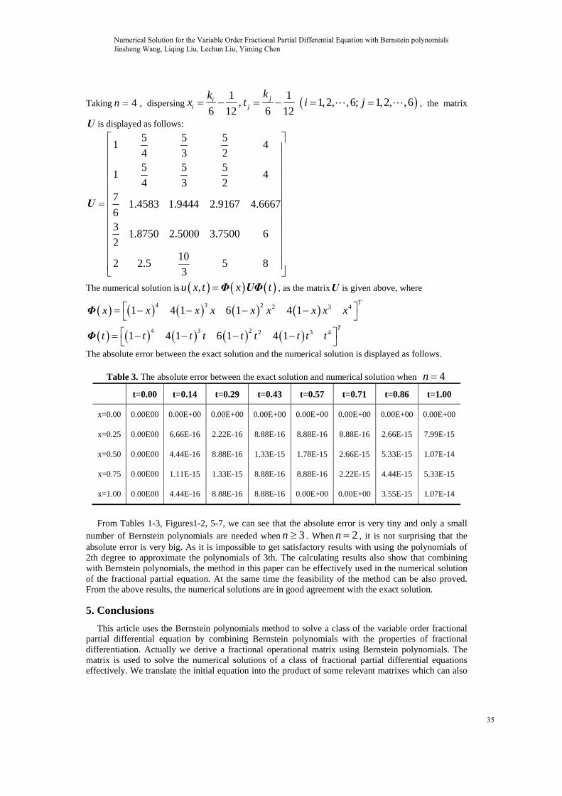
Taking 4n , dispersing 1 1, 1,2, 5; 1,2, 5
5 10 5 10ji
i j i j
kkx t k k , the matrix
U is displayed as follows:
0 0 0 0 0
0 0 0 0 0
52.5000 3.6111 5 6.6667
35
3.7500 5.4167 7.5000 1020 0 0 0 0
U
Numerical Solution for the Variable Order Fractional Partial Differential Equation with Bernstein polynomials Jinsheng Wang, Liqing Liu, Lechun Liu, Yiming Chen
29
The numerical solution is ,u x t x tΦ UΦ , as the matrixU is given above, and
4 3 2 2 3 41 4 1 6 1 4 1 ,T
x x x x x x x x x Φ
4 3 2 2 3 41 4 1 6 1 4 1T
t t t t t t t t t Φ .
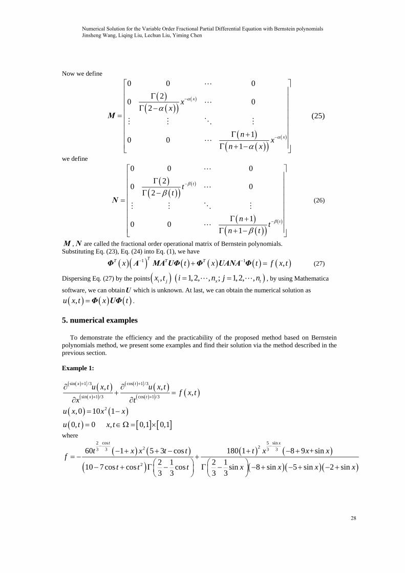
The absolute error between the exact solution and the numerical solution is displayed as follows:
Figure 2. The absolute error for Example 1 of 4n
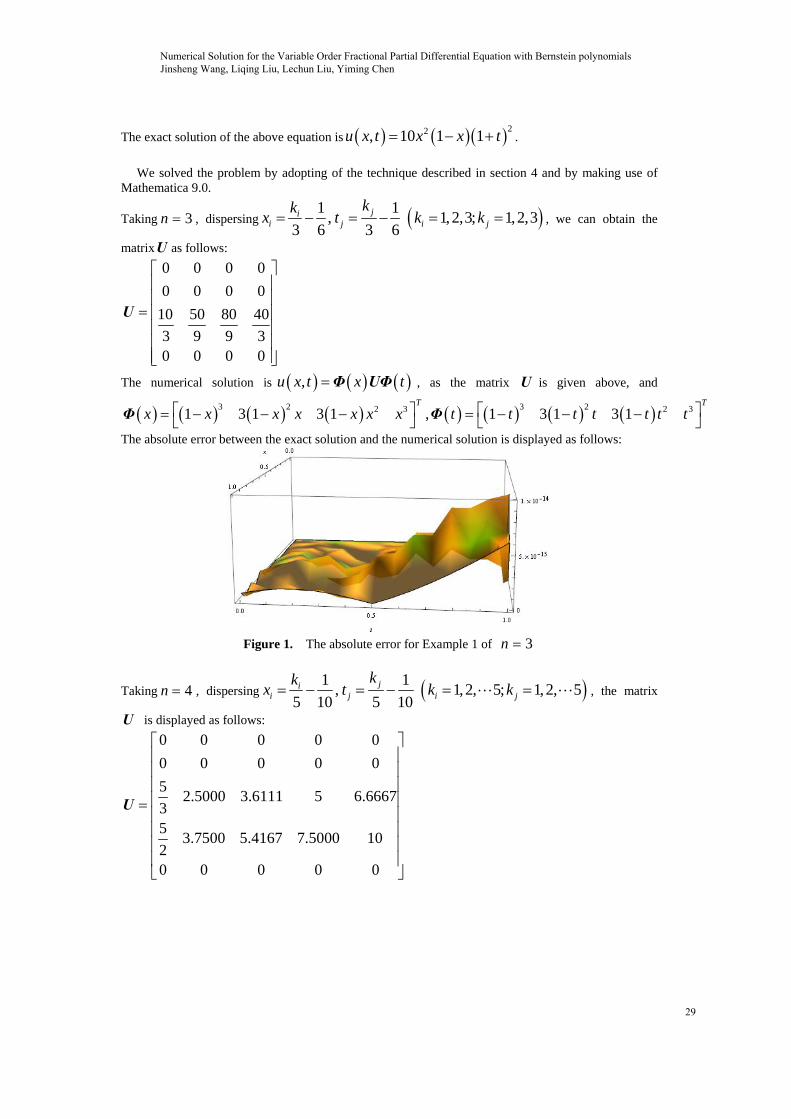
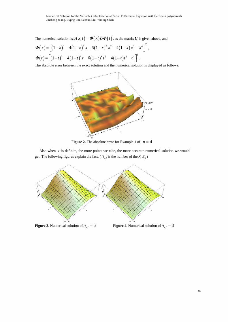
Also when n is definite, the more points we take, the more accurate numerical solution we would
get. The following figures explain the fact. ( ,x tn is the number of the ,i jx t )
Figure 3. Numerical solution of , 5x tn Figure 4. Numerical solution of , 8x tn
Numerical Solution for the Variable Order Fractional Partial Differential Equation with Bernstein polynomials Jinsheng Wang, Liqing Liu, Lechun Liu, Yiming Chen
30
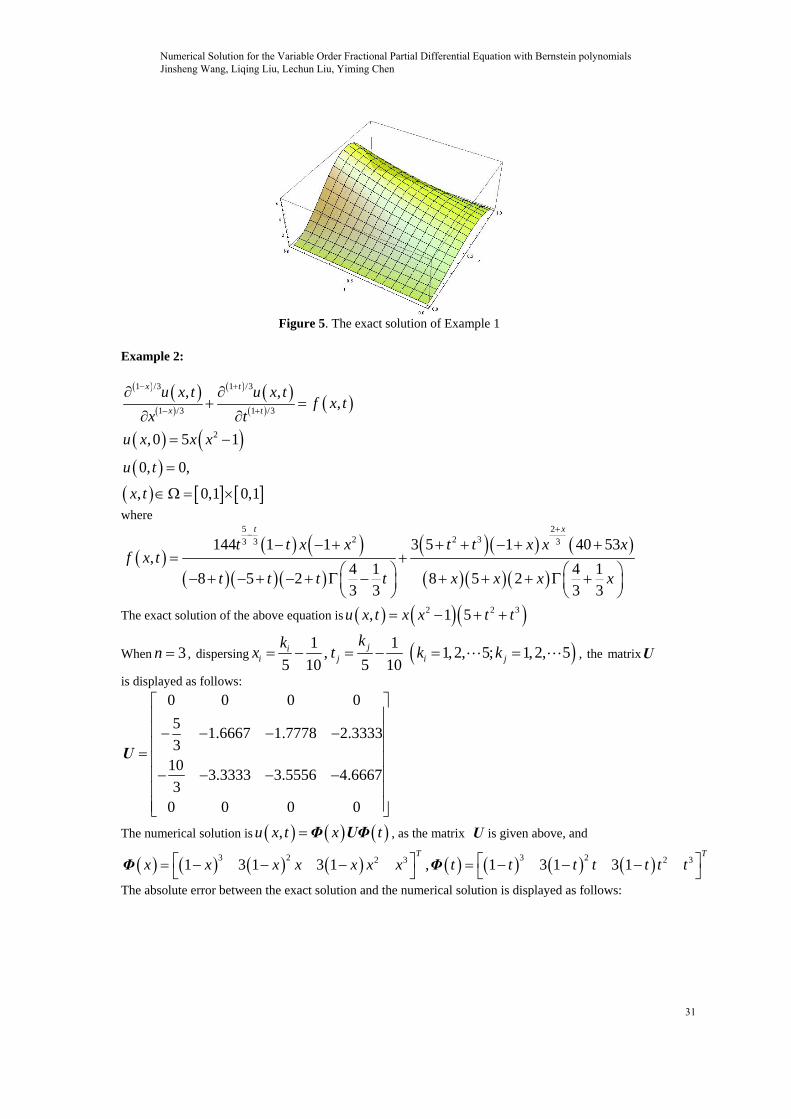
Figure 5. The exact solution of Example 1
Example 2:
1 /3 1 /3
1 /3 1 /3
2
, ,,
,0 5 1
0, 0,
, 0,1 0,1
x t
x t
u x t u x tf x t
x t
u x x x
u t
x t
where
5 22 2 33 3 3144 1 1 3 5 1 40 53
,4 1 4 1
8 5 2 8 5 23 3 3 3
t x
t t x x t t x x xf x t
t t t t x x x x
The exact solution of the above equation is 2 2 3, 1 5u x t x x t t
When 3n , dispersing 1 1, 1,2, 5; 1,2, 5
5 10 5 10ji
i j i j
kkx t k k , the matrixU
is displayed as follows:
0 0 0 0
51.6667 1.7778 2.3333
310
3.3333 3.5556 4.66673
0 0 0 0
U
The numerical solution is ,u x t x tΦ UΦ , as the matrix U is given above, and
3 2 3 22 3 2 31 3 1 3 1 , 1 3 1 3 1T T
x x x x x x x t t t t t t t Φ Φ
The absolute error between the exact solution and the numerical solution is displayed as follows:
Numerical Solution for the Variable Order Fractional Partial Differential Equation with Bernstein polynomials Jinsheng Wang, Liqing Liu, Lechun Liu, Yiming Chen
31
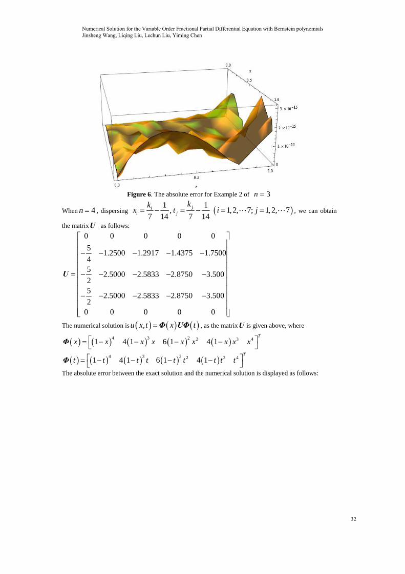
Figure 6. The absolute error for Example 2 of 3n
When 4n , dispersing 1 1, 1,2, 7; 1,2, 7
7 14 7 14ji
i j
kkx t i j , we can obtain
the matrixU as follows:
0 0 0 0 0
51.2500 1.2917 1.4375 1.7500
45
2.5000 2.5833 2.8750 3.50025
2.5000 2.5833 2.8750 3.5002
0 0 0 0 0
U
The numerical solution is ,u x t x tΦ UΦ , as the matrixU is given above, where
4 3 2 2 3 41 4 1 6 1 4 1T
x x x x x x x x x Φ
4 3 2 2 3 41 4 1 6 1 4 1T
t t t t t t t t t Φ
The absolute error between the exact solution and the numerical solution is displayed as follows:
Numerical Solution for the Variable Order Fractional Partial Differential Equation with Bernstein polynomials Jinsheng Wang, Liqing Liu, Lechun Liu, Yiming Chen
32
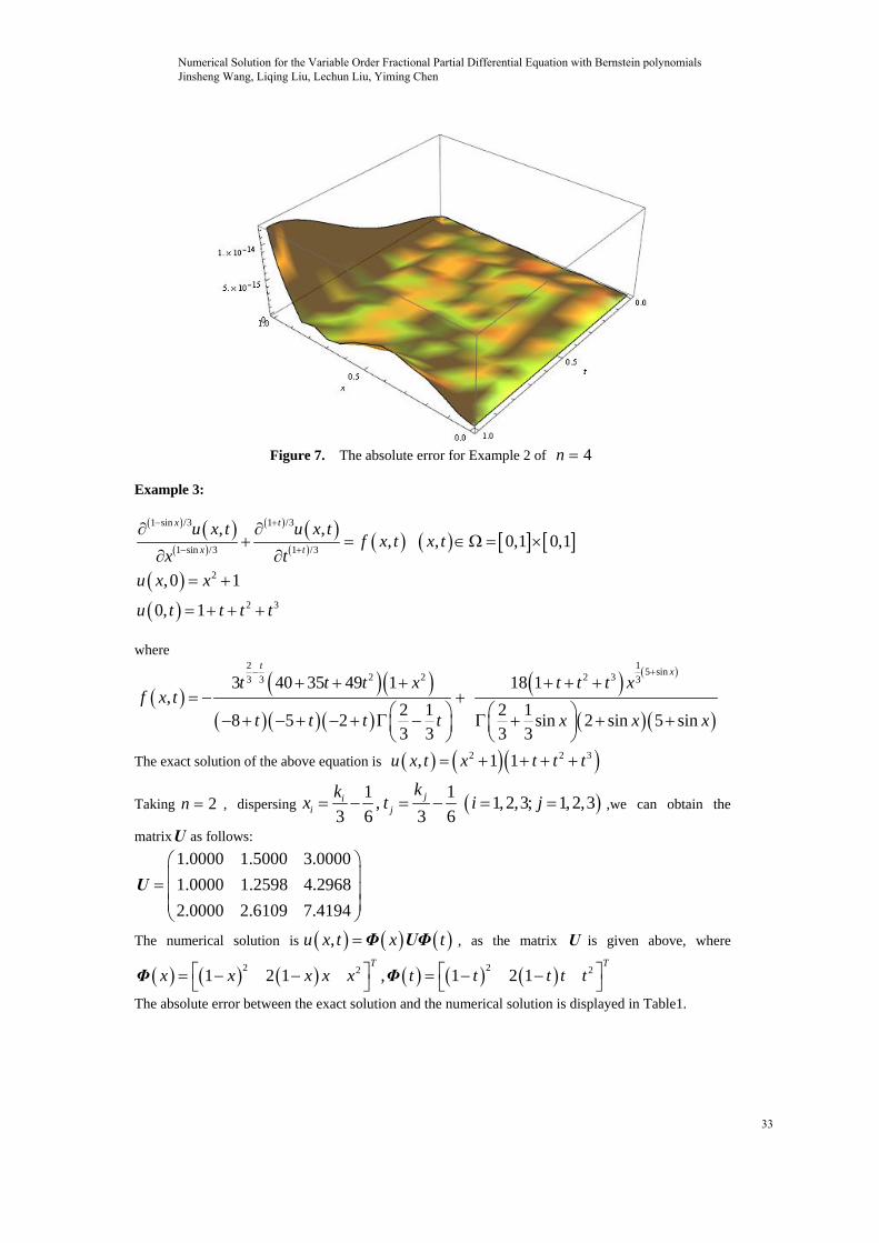
Figure 7. The absolute error for Example 2 of 4n
Example 3:
1 sin /3 1 /3
1 sin /3 1 /3
2
2 3
, ,, , 0,1 0,1
,0 1
0, 1
x t
x t
u x t u x tf x t x t
x t
u x x
u t t t t
where
2 15 sin2 2 2 33 3 33 40 35 49 1 18 1
,2 1 2 1
8 5 2 sin 2 sin 5 sin3 3 3 3
tx
t t t x t t t xf x t
t t t t x x x
The exact solution of the above equation is 2 2 3, 1 1u x t x t t t
Taking 2n , dispersing 1 1, 1,2,3; 1,2,3
3 6 3 6ji
i j
kkx t i j ,we can obtain the
matrixU as follows:
1.0000 1.5000 3.0000
1.0000 1.2598 4.2968
2.0000 2.6109 7.4194
U
The numerical solution is ,u x t x tΦ UΦ , as the matrix U is given above, where
2 22 21 2 1 , 1 2 1T T
x x x x x t t t t t Φ Φ
The absolute error between the exact solution and the numerical solution is displayed in Table1.
Numerical Solution for the Variable Order Fractional Partial Differential Equation with Bernstein polynomials Jinsheng Wang, Liqing Liu, Lechun Liu, Yiming Chen
33
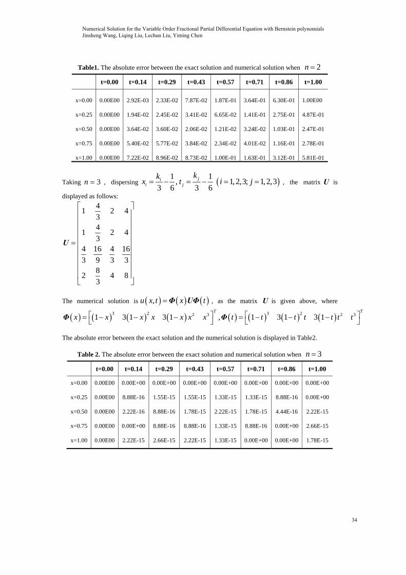
Table1. The absolute error between the exact solution and numerical solution when 2n
t=0.00 t=0.14 t=0.29 t=0.43 t=0.57 t=0.71 t=0.86 t=1.00
x=0.00 0.00E00 2.92E-03 2.33E-02 7.87E-02 1.87E-01 3.64E-01 6.30E-01 1.00E00
x=0.25 0.00E00 1.94E-02 2.45E-02 3.41E-02 6.65E-02 1.41E-01 2.75E-01 4.87E-01
x=0.50 0.00E00 3.64E-02 3.60E-02 2.06E-02 1.21E-02 3.24E-02 1.03E-01 2.47E-01
x=0.75 0.00E00 5.40E-02 5.77E-02 3.84E-02 2.34E-02 4.01E-02 1.16E-01 2.78E-01
x=1.00 0.00E00 7.22E-02 8.96E-02 8.73E-02 1.00E-01 1.63E-01 3.12E-01 5.81E-01
Taking 3n , dispersing 1 1, 1,2,3; 1,2,3
3 6 3 6ji
i j
kkx t i j , the matrix U is
displayed as follows:
41 2 4
34
1 2 43
4 16 4 16
3 9 3 38
2 4 83
U
The numerical solution is ,u x t x tΦ UΦ , as the matrix U is given above, where
3 2 3 22 3 2 31 3 1 3 1 , 1 3 1 3 1T T
x x x x x x x t t t t t t t Φ Φ
The absolute error between the exact solution and the numerical solution is displayed in Table2.
Table 2. The absolute error between the exact solution and numerical solution when 3n
t=0.00 t=0.14 t=0.29 t=0.43 t=0.57 t=0.71 t=0.86 t=1.00
x=0.00 0.00E00 0.00E+00 0.00E+00 0.00E+00 0.00E+00 0.00E+00 0.00E+00 0.00E+00
x=0.25 0.00E00 8.88E-16 1.55E-15 1.55E-15 1.33E-15 1.33E-15 8.88E-16 0.00E+00
x=0.50 0.00E00 2.22E-16 8.88E-16 1.78E-15 2.22E-15 1.78E-15 4.44E-16 2.22E-15
x=0.75 0.00E00 0.00E+00 8.88E-16 8.88E-16 1.33E-15 8.88E-16 0.00E+00 2.66E-15
x=1.00 0.00E00 2.22E-15 2.66E-15 2.22E-15 1.33E-15 0.00E+00 0.00E+00 1.78E-15
Numerical Solution for the Variable Order Fractional Partial Differential Equation with Bernstein polynomials Jinsheng Wang, Liqing Liu, Lechun Liu, Yiming Chen
34
Taking 4n , dispersing 1 1, 1,2, ,6; 1,2, ,6
6 12 6 12ji
i j
kkx t i j , the matrix
U is displayed as follows:
5 5 51 4
4 3 25 5 5
1 44 3 2
71.4583 1.9444 2.9167 4.6667
63
1.8750 2.5000 3.7500 62
102 2.5 5 8
3
U
The numerical solution is ,u x t x tΦ UΦ , as the matrixU is given above, where
4 3 2 2 3 41 4 1 6 1 4 1T
x x x x x x x x x Φ
4 3 2 2 3 41 4 1 6 1 4 1T
t t t t t t t t t Φ
The absolute error between the exact solution and the numerical solution is displayed as follows.
Table 3. The absolute error between the exact solution and numerical solution when 4n t=0.00 t=0.14 t=0.29 t=0.43 t=0.57 t=0.71 t=0.86 t=1.00
x=0.00 0.00E00 0.00E+00 0.00E+00 0.00E+00 0.00E+00 0.00E+00 0.00E+00 0.00E+00
x=0.25 0.00E00 6.66E-16 2.22E-16 8.88E-16 8.88E-16 8.88E-16 2.66E-15 7.99E-15
x=0.50 0.00E00 4.44E-16 8.88E-16 1.33E-15 1.78E-15 2.66E-15 5.33E-15 1.07E-14
x=0.75 0.00E00 1.11E-15 1.33E-15 8.88E-16 8.88E-16 2.22E-15 4.44E-15 5.33E-15
x=1.00 0.00E00 4.44E-16 8.88E-16 8.88E-16 0.00E+00 0.00E+00 3.55E-15 1.07E-14
From Tables 1-3, Figures1-2, 5-7, we can see that the absolute error is very tiny and only a small
number of Bernstein polynomials are needed when 3n . When 2n , it is not surprising that the absolute error is very big. As it is impossible to get satisfactory results with using the polynomials of 2th degree to approximate the polynomials of 3th. The calculating results also show that combining with Bernstein polynomials, the method in this paper can be effectively used in the numerical solution of the fractional partial equation. At the same time the feasibility of the method can be also proved. From the above results, the numerical solutions are in good agreement with the exact solution.
5. Conclusions This article uses the Bernstein polynomials method to solve a class of the variable order fractional
partial differential equation by combining Bernstein polynomials with the properties of fractional differentiation. Actually we derive a fractional operational matrix using Bernstein polynomials. The matrix is used to solve the numerical solutions of a class of fractional partial differential equations effectively. We translate the initial equation into the product of some relevant matrixes which can also
Numerical Solution for the Variable Order Fractional Partial Differential Equation with Bernstein polynomials Jinsheng Wang, Liqing Liu, Lechun Liu, Yiming Chen
35
be regarded as the system of linear equations after dispersing the variable. And it is easy to solve by the least square method. Numerical examples illustrate the powerful of the proposed method. The solutions obtained using the suggested method show that numerical solutions are in very good coincidence with the exact solution. The method can be applied by developing for the other fractional problem.
However, there are many issues to be resolved, such as the section 1 0,1 0,1 is
transformed to 2 0, 0,X T , or the equations are nonlinear and so on. This requires the
efforts of all of us.
6. Acknowledgement: [1] This work is supported by the Natural Foundation of Hebei Province (A2012203407). [2] This work is supported by Qinhuangdao research and development program of science and
technology, Adaptive Boundary Element Method of precision rolling process simulation. (201201B019)
[3] This work is supported by Qinhuangdao Technology Bureau 2013 research and development projects of science and technology. (201302A023)
The authors also gratefully acknowledge the helpful comments and suggestions of the reviewers, which have improved the presentation.
7. References [1] Leda Galue, S.L. Kalla, B.N. Al-Saqabi, “Fractional extensions of the temperature field problems
in oil strata”, Applied Mathematics and Computation, Elsevier, vol. 186, no.1, pp. 35–44, 2007. [2] I. L. EI-Kalla, “Error estimate of the series solution to a class of nonlinear fractional differential
equations”. Commun. Nonlinear Sci. Numer. Simulate, Elsevier, vol. 16, no.3, pp. 1408-1413, 2011.
[3] Ahmed. M. A. EI-Sayed, “Nonlinear functional differential equations of arbitrary orders”. Nonliear Analysis: Theory, Methods & Applications, Elsevier, vol. 33, no.2, pp. 181-186, 1998.
[4] Zaid. Odibat, “A study on the convergence of variational iteration method”, Mathematical and Computer Modelling, Elsevier, vol.51, no. 9-10, pp. 1181-1192, 2010.
[5] Shaher Momani, Zaid. Odibat, “Generalized differential transform method for solving a space and time-fractional diffusion-wave equation”, Physics Letters A, Elsevier, vol.370, no. 5-6, pp. 379-387, 2007.
[6] Zaid. Odibat, Shaher Momani, “A generalized differential transform method for linear partial differential equations of fractional order”, Applied Mathematics Letters, Elsevier, vol. 21, no. 2, pp. 194-199, 2008.
[7] Zaid. Odibat, Shaher Momani, “Generalized differential transform method: Application to differential equations of fractional order”, Applied Mathematics and Computation, Elsevier, vol. 197, no.2, pp. 467-477, 2008.
[8] Yuanlu Li, Ning Sun, “Numerical solution of fractional differential equations using the generalized block pulse operational matrix”, Computers and Mathematics with Application, Elsevier, vol. 62, no.3, pp. 1046 -1054, 2011.
[9] Li Zhu, Qibin Fan, “Solving fractional nonlinear Fredholm integro-differential equations by the second kind Chebyshev wavelet”. Communications in Nonlinear Science and Numerical Simulatation, Elsevier, vol. 17, no.6, pp. 2333-2341, 2012.
[10] Mingxu Yi, Yiming Chen, “Haar wavelet operational matrix method for solving fractional partial differential equations”. Computer Modeling in Engineering &Sciences, Tech Science, vol. 88, no.3, pp. 229-244, 2012.
[11] Zaid. Odibat, Shaher Momani, “An algorithm for the numerical solution of differential equations of fractional order”, J. Appl. Math. Inform, Elsevier, vol. 26, no. 1-2, pp. 15–27, 2008.
[12] Kai Diethelm, Neville J. Ford, “Multi-order fractional differential equations and their numerical solution”, Applied Mathematics and Computation, Elsevier, vol. 154, no.3, pp. 621–640, 2004.
[13] M. Javidi, A. Golbabai, “Modified homotopy perturbation method for solving system of linear
Numerical Solution for the Variable Order Fractional Partial Differential Equation with Bernstein polynomials Jinsheng Wang, Liqing Liu, Lechun Liu, Yiming Chen
36
Fredholm integral equations”, Mathematical and Computer Modelling, Elsevier, vol. 50, no. 1-2, pp. 159-165, 2009.
[14] Lorenzo Carl F, Hartley Tom T, “Initialization, conceptualization, and application in the generalized fractional calculus”, Critical Reviews in Biomedical Engineering, PubMed, vol. 35, no.6, pp.447-553, 2007.
[15] Zaid. Odibat, Shaher Momani, “Generalized differential transform method for solving a space and time-fractional diffusion-wave equation”, Physics Letters A, Elsevier, vol.370, no. 5-6, pp. 379-387, 2007.
[16] C.F.M. Coimbra, “Mechanics with variable-order differential operators”, Ann. Phys, General & Introductory Physics , vol.12, no. 11–12, pp. 692–703, 2003.
[17] Stefan G. Samko, Bertram Ross, “Intergation and differentiation to a variable fractional order”, Integral Transforms and Special Functions, Taylor & Francis, vol. 1, no. 4, pp. 277–300, 1993.
[18] S.G. Samko, “Fractional integration and differentiation of variable order”, Analysis Mathematica, Springer, vol. 21, no. 3, pp. 213–236, 1995.
[19] C.M. Soon, F.M. Coimbra, M.H. Kobayashi, “The variable viscoelasticity oscillator”, Ann. Phys., Wiley, vol. 12, no. 11-12, pp. 692-703, 2003.
[20] R. Lin, F. Liu, V. Anh, I. Turner, “Stability and convergence of a new explicit finite-difference approximation for the variable-order nonlinear fractional diffusion equation”, Applied Mathematics and Computation, Elsevier, vol. 212, no. 2, pp. 435–445, 2009.
[21] P. Zhuang, F. Liu, V. Anh, I. Turner, “Numerical methods for the variable-order fractional advection-diffusion equation with a nonlinear source term”, SIAM J. Numer. Anal, Society for Industrial and Applied Mathematics Philadelphia, PA, USA, vol. 47, no.3, pp. 1760–1781, 2009.
[22] Chang-Ming Chen, Fawang Liu, Vo Anh, Ian W. Turner, “Numerical schemes with high spatial accuracy for a variable-order anomalous subdiffusion equation”, SIAM J. Sci. Comput, The DBLP Computer Science Bibliography, vol. 32, no. 4, pp. 1740–1760, 2010.
[23] S.A. Yousefi, M. Behroozifar, Mehdi Dehghan, “The operational matrices of Bernstein polynomials for solving the parabolic equation subject to specification of the mass”. Journal of Computational and Applied Mathematics, Elsevier, vol. 235, no.17, pp. 5272–5283, 2011.
[24] S.A. Yousefi, M. Behroozifar, “Operational matrices of Bernstein polynomials and their applications”, Internat. J. Systems Sci, Elsevier, vol. 41, no. 6, pp. 709–716, 2010.
[25] Yiming Chen, Mingxu Yi, Chen Chen, Chunxiao Yu, “Bernstein polynomials method for fractional convection-diffusion equation with variable coefficients”, Computer Modeling in Engineering & Sciences, Tech Science, vol. 83, no.6, pp. 639-653, 2011.
[26] E.H. Doha, A.H. Bhrawy, M.A. Saker, “Integrals of Bernstein polynomials: an application for the solution of high even-order differential equations”, Applied Mathematics Letters, Elsevier, vol. 24, no. 4, pp. 559–565, 2011.
[27] K. Maleknejad, E. Hashemizadeh, B. Basirat, “Computational method based on Bernstein operational matrices for nonlinear Volterra–Fredholm–Hammerstein integral equations”, Commun Nonlinear Sci Numer Simulat, Elsevier, vol.17, no. 1, pp. 52–61, 2012.
[28] Maleknejad K, Hashemizadeh E, Ezzati R, “A new approach to the numerical solution of Volterra integral equations by using Bernsteins approximation”, Commun Nonlinear Sci Numer Simulat, Elsevier, vol.16, no. 2, pp. 647–655, 2011.
[29] Mandal BN, Bhattacharya S, “Numerical solution of some classes of integral equations using Bernstein polynomials”, Applied Mathematics and Computation, Elsevier, vol. 190, no. 2, pp. 1707–16, 2007.
Numerical Solution for the Variable Order Fractional Partial Differential Equation with Bernstein polynomials Jinsheng Wang, Liqing Liu, Lechun Liu, Yiming Chen
37

![Fractional Cascading Fractional Cascading I: A Data Structuring Technique Fractional Cascading II: Applications [Chazaelle & Guibas 1986] Dynamic Fractional](https://img.pdfslide.us/doc/110x75/56649ea25503460f94ba64dd/fractional-cascading-fractional-cascading-i-a-data-structuring-technique-fractional.jpg)