Linear and nonlinear diffusion with fractional operators · The fractional Laplacian operator Different formulas for fractional Laplacian operator. We assume that the space variable

$Page 1: Linear and nonlinear diffusion with fractional operators · The fractional Laplacian operator Different formulas for fractional Laplacian operator. We assume that the space variable$
1

Linear and nonlinear diffusion with fractionaloperators

JUAN LUIS VAZQUEZ

Departamento de MatematicasUniversidad Autonoma de Madridand Royal Academy of Sciences

BCAM Scientific SeminarBilbao, 29 Nov. 2016

2

Outline

1 Linear and Nonlinear DiffusionNonlinear equations

2 Fractional diffusion

3 Nonlinear Fractional diffusion modelsModel I. A potential Fractional diffusionMain estimates for this model

4 Recent team work

5 Operators and Equations in Bounded Domains

3

Outline




4 Recent team work


Outline




4 Recent team work


5

Diffusion equations describe how a continuous medium(say, a population) spreads to occupy the available space.Models come from all kinds of applications: fluids,chemicals, bacteria, animal populations, the stock market,...These equations have occupied a large part of my research since 1980.

The mathematical study of diffusion starts with the HeatEquation,

ut = ∆ua linear example of immense influence in Science.The Heat Equation has produced a huge number of concepts,techniques and connections for pure and applied science, for analysts,probabilists, computational people and geometers, for physicists andengineers, and lately in finance and the social sciences.Today educated people talk about the Gaussian function, separation ofvariables, Fourier analysis, spectral decomposition, Dirichlet forms,Maximum Principles, Brownian motion, generation of semigroups,positive operators in Banach spaces, entropy dissipation, ...

5




5




5




6

Nonlinear equations

The heat example is generalized into the theory of linear parabolicequations, which is nowadays a basic topic in any advanced study ofPDEs.However, the heat example and the linear models are not representativeenough, since many models of science are nonlinear in a form that isvery not-linear. A general model of nonlinear diffusion takes thedivergence form

∂tH(u) = ∇ · ~A(x, u,Du) + B(x, t, u,Du)

with monotonicity conditions on H and ∇p ~A(x, t, u, p) and structuralconditions on ~A and B. Posed in the 1960s (Serrin et al.)In this generality the mathematical theory is too rich to admit a simpledescription. This includes the big areas of Nonlinear Diffusion andReaction Diffusion, where I have been working.Reference works. Books by Ladyzhenskaya-Solonnikov-Uraltseva,Friedman, Smoller,... But they are only basic reference.

6

Nonlinear equations


∂tH(u) = ∇ · ~A(x, u,Du) + B(x, t, u,Du)


6

Nonlinear equations


∂tH(u) = ∇ · ~A(x, u,Du) + B(x, t, u,Du)


7

Nonlinear heat flows

Many specific examples, now considered the “classical nonlineardiffusion models”, have been investigated to understand in detail thequalitative features and to introduce the quantitative techniques, thathappen to be many and from very different originsTypical nonlinear diffusion: Stefan Problem (phase transition betweentwo fluids like ice and water), Hele-Shaw Problem (potential flow in athin layer between solid plates), Porous Medium Equation:ut = ∆(um), Evolution P-Laplacian Eqn: ut = ∇ · (|∇u|p−2∇u).

Typical reaction diffusion: Fujita model ut = ∆u + up.

7




7




8

Outline




4 Recent team work


9

Recent Direction. Fractional diffusion

Replacing Laplacians by fractional Laplacians is motivated by the need torepresent anomalous diffusion. In probabilistic terms, it replacesnext-neighbour interaction of Random Walks and their limit, the Brownianmotion, by long-distance interaction. The main mathematical models are theFractional Laplacians that have special symmetry and invariance properties.

The Basic evolution equation

ut + (−∆)su = 0

Intense work in Stochastic Processes for some decades, but not in Analysis ofPDEs until 10 years ago, initiated around Prof. Caffarelli in Texas.

A basic theory and survey for PDE people: M. Bonforte, Y. Sire, J. L. Vazquez.“Optimal Existence and Uniqueness Theory for the Fractional Heat Equation”,Arxiv:1606.00873v1 [math.AP], to appear.

Precedent : B. Barrios, I. Peral, F. Soria, E. Valdinoci. “A Widder’s typetheorem for the heat equation with nonlocal diffusion” Arch. Ration. Mech.Anal. 213 (2014), no. 2, 629–650.

9




ut + (−∆)su = 0




9




ut + (−∆)su = 0




10

The fractional Laplacian operator

Different formulas for fractional Laplacian operator.We assume that the space variable x ∈ Rn, and the fractional exponentis 0 < s < 1. First, pseudo differential operator given by the Fourier transform:

(−∆)su(ξ) = |ξ|2su(ξ)

Singular integral operator:

(−∆)su(x) = Cn,s

∫Rn

u(x)− u(y)

|x− y|n+2s dy

With this definition, it is the inverse of the Riesz integral operator (−∆)−su.This one has kernel C1|x− y|n−2s, which is not integrable.Take the random walk for Levy processes:

un+1j =

∑k

Pjkunk

where Pik denotes the transition function which has a . tail (i.e, power decaywith the distance |i− k|). In the limit you get an operator A as the infinitesimalgenerator of a Levy process: if Xt is the isotropic α-stable Levy process we have

Au(x) = limh→0

E(u(x)− u(x + Xh))

10



(−∆)su(ξ) = |ξ|2su(ξ)


(−∆)su(x) = Cn,s

∫Rn

u(x)− u(y)

|x− y|n+2s dy


un+1j =

∑k

Pjkunk


Au(x) = limh→0

E(u(x)− u(x + Xh))

10



(−∆)su(ξ) = |ξ|2su(ξ)


(−∆)su(x) = Cn,s

∫Rn

u(x)− u(y)

|x− y|n+2s dy


un+1j =

∑k

Pjkunk


Au(x) = limh→0

E(u(x)− u(x + Xh))

11

The fractional Laplacian operator II

The α-harmonic extension: Find first the solution of the (n + 1) problem

∇ · (y1−α∇v) = 0 (x, y) ∈ Rn × R+; v(x, 0) = u(x), x ∈ Rn.

Then, putting α = 2s we have

(−∆)su(x) = −Cα limy→0

y1−α ∂v∂y

When s = 1/2 i.e. α = 1, the extended function v is harmonic (in n + 1variables) and the operator is the Dirichlet-to-Neumann map on the base spacex ∈ Rn. It was proposed in PDEs by Caffarelli and Silvestre, 2007.This construction is generalized to other differential operators, like theharmonic oscillator, by Stinga and Torrea, Comm. PDEs, 2010.

The semigroup formula in terms of the heat flow generated by ∆:

(−∆)sf (x) =1

Γ(−s)

∫ ∞0

(et∆f (x)− f (x)

) dtt1+s .

11

The fractional Laplacian operator II

The α-harmonic extension: Find first the solution of the (n + 1) problem

∇ · (y1−α∇v) = 0 (x, y) ∈ Rn × R+; v(x, 0) = u(x), x ∈ Rn.

Then, putting α = 2s we have

(−∆)su(x) = −Cα limy→0

y1−α ∂v∂y

When s = 1/2 i.e. α = 1, the extended function v is harmonic (in n + 1variables) and the operator is the Dirichlet-to-Neumann map on the base spacex ∈ Rn. It was proposed in PDEs by Caffarelli and Silvestre, 2007.This construction is generalized to other differential operators, like theharmonic oscillator, by Stinga and Torrea, Comm. PDEs, 2010.

The semigroup formula in terms of the heat flow generated by ∆:

(−∆)sf (x) =1

Γ(−s)

∫ ∞0

(et∆f (x)− f (x)

) dtt1+s .

12

Fractional Laplacians on bounded domainsIn Rn all the previous versions are equivalent. In a bounded domain Ω ⊂ Rn we haveto re-examine all of them. Two main alternatives are studied in probability and PDEs,corresponding to different options about what happens to particles at the boundary orwhat is the domain of the functionals. There are more alternatives.

The restricted Laplacian. It is the simplest option. Functions f (x) defined in Ωare extended by zero to the complement and then the whole space hypersingularintegral is used

(−∆rest)sf (x) = cn,sP.V.

∫Rn

f (x)− f (y)

|x− y|n+2s dy.

The spectral Laplacian

(−∆sp)sf (x) =

1Γ(−s)

∫ ∞0

(et∆D f (x)− f (x)

) dtt1+s =

∞∑j=1

λsj fj ϕj(x) ,

where (λj, ϕj), j = 1, 2, . . . are the normalized spectral sequence of thestandard Dirichlet Laplacian ∆D on Ω, fj are the Fourier coeff. of f .

Analysis references for the whole space. Books by Landkof (1966-72), Stein (1970),Davies (1996). Analysis references for Bounded Domains. Cabre, Bonforte, Grubb,Musina, Sire, Vazquez, Valdinoci,...

12

Fractional Laplacians on bounded domainsIn Rn all the previous versions are equivalent. In a bounded domain Ω ⊂ Rn we haveto re-examine all of them. Two main alternatives are studied in probability and PDEs,corresponding to different options about what happens to particles at the boundary orwhat is the domain of the functionals. There are more alternatives.

The restricted Laplacian. It is the simplest option. Functions f (x) defined in Ωare extended by zero to the complement and then the whole space hypersingularintegral is used

(−∆rest)sf (x) = cn,sP.V.

∫Rn

f (x)− f (y)

|x− y|n+2s dy.

The spectral Laplacian

(−∆sp)sf (x) =

1Γ(−s)

∫ ∞0

(et∆D f (x)− f (x)

) dtt1+s =

∞∑j=1

λsj fj ϕj(x) ,

where (λj, ϕj), j = 1, 2, . . . are the normalized spectral sequence of thestandard Dirichlet Laplacian ∆D on Ω, fj are the Fourier coeff. of f .

Analysis references for the whole space. Books by Landkof (1966-72), Stein (1970),Davies (1996). Analysis references for Bounded Domains. Cabre, Bonforte, Grubb,Musina, Sire, Vazquez, Valdinoci,...

13

Mathematical theory of the Fractional Heat Equation

The Linear Problem isut + (−∆)s(u) = 0

We take x ∈ Rn, 0 < m <∞, 0 < s < 1, with initial data in u0 ∈ L1(Rn).Normally, u0, u ≥ 0.This model represents the linear flow generated by the so-called Levy processesin Stochastic PDEs, where the transition from one site xj of the mesh to anothersite xk has a probability that depends on the distance |xk − xj| in the form of aninverse power for j 6= k. The power we take is c |xk − xj|−n−2s. The range is0 < s < 1. The limit from random walk to the continuous equation is done byE. Valdinoci, in From the long jump random walk to the fractional Laplacian,Bol. Soc. Esp. Mat. Apl. 49 (2009), 33-44.The solution of the linear equation can be obtained in Rn by means ofconvolution with the fractional heat kernel

u(x, t) =

∫u0(y)Pt(x− y) dy,

and people in probability (like Blumental and Getoor) proved in the 1960s that

Pt(x) t(t1/s + |x|2

)(n+2s)/2 ⇒ look at the fat tail.

13




u(x, t) =



Pt(x) t(t1/s + |x|2


13




u(x, t) =



Pt(x) t(t1/s + |x|2


14

The paperB. Barrios, I. Peral, F. Soria, E. Valdinoci. “A Widder’s type theorem for theheat equation with nonlocal diffusion” Arch. Ration. Mech. Anal. 213 (2014),no. 2, 629-650, studies the theory in classes of (maybe) large functions andstudies the question: is every solution representable by the convolution formula.The answer is yes if the solutions are ‘nice’ strong solutions and the growth in xis no more that u(x, t) ≤ (1 + |x|)a with a < 2s.

Our recent paperM. Bonforte, Y. Sire, J. L. Vazquez. “Optimal Existence and UniquenessTheory for the Fractional Heat Equation”, Arxiv:1606.00873v1solves the problem of existence and uniqueness of solutions when the initialdata is a locally finite Radon measure with the condition∫

Rn(1 + |x|)−(n+2s) dµ(x) <∞ . (1)

Moreover we prove that any constructed solution by convolution, or any veryweak solution u ≥ 0, has an initial trace µ which is a measure in the above classMs. So the result closes the problem of the Widder theory for the fractionalheat equation posed in Rn.

The paper goes on to tell what you want to know about this semigroup fornonnegative solutions. Arxiv is free.

14



Rn(1 + |x|)−(n+2s) dµ(x) <∞ . (1)



14



Rn(1 + |x|)−(n+2s) dµ(x) <∞ . (1)



14



Rn(1 + |x|)−(n+2s) dµ(x) <∞ . (1)



15

Recent coauthors

16

Outline




4 Recent team work


17

Nonlocal nonlinear diffusion model I

The model arises from the consideration of a continuum, say, a fluid,represented by a density distribution u(x, t) ≥ 0 that evolves with timefollowing a velocity field v(x, t), according to the continuity equation

ut +∇ · (u v) = 0.

We assume next that v derives from a potential, v = −∇p, as happens in fluidsin porous media according to Darcy’s law, an in that case p is the pressure. Butpotential velocity fields are found in many other instances, like Hele-Shawcells, and other recent examples.

We still need a closure relation to relate u and p. In the case of gases in porousmedia, as modeled by Leibenzon and Muskat, the closure relation takes theform of a state law p = f (u), where f is a nondecreasing scalar function, whichis linear when the flow is isothermal, and a power of u if it is adiabatic.The linear relationship happens also in the simplified description of waterinfiltration in an almost horizontal soil layer according to Boussinesq. In bothcases we get the standard porous medium equation, ut = c∆(u2).See PME Book for these and other applications (around 20!).

17



ut +∇ · (u v) = 0.



17



ut +∇ · (u v) = 0.



17



ut +∇ · (u v) = 0.



18

Nonlocal diffusion model. The problemThe diffusion model with nonlocal effects proposed in 2007 with LuisCaffarelli uses the derivation of the PME but with a closure relation of the formp = K(u), where K is a linear integral operator, which we assume in practiceto be the inverse of a fractional Laplacian. Hence, p es related to u through afractional potential operator, K = (−∆)−s, 0 < s < 1, with kernel

k(x, y) = c|x− y|−(n−2s)

(i.e., a Riesz operator). We have (−∆)sp = u.

The diffusion model with nonlocal effects is thus given by the system

ut = ∇ · (u∇p), p = K(u). (2)

where u is a function of the variables (x, t) to be thought of as a density orconcentration, and therefore nonnegative, while p is the pressure, which isrelated to u via a linear operator K. ut = ∇ · (u∇(−∆)−su)

The problem is posed for x ∈ Rn, n ≥ 1, and t > 0, and we give initialconditions

u(x, 0) = u0(x), x ∈ Rn, (3)

where u0 is a nonnegative, bounded and integrable function in Rn.Papers and surveys by us and others are available, see below

18


k(x, y) = c|x− y|−(n−2s)



ut = ∇ · (u∇p), p = K(u). (2)



u(x, 0) = u0(x), x ∈ Rn, (3)


18


k(x, y) = c|x− y|−(n−2s)



ut = ∇ · (u∇p), p = K(u). (2)



u(x, 0) = u0(x), x ∈ Rn, (3)


18


k(x, y) = c|x− y|−(n−2s)



ut = ∇ · (u∇p), p = K(u). (2)



u(x, 0) = u0(x), x ∈ Rn, (3)


19

Nonlocal diffusion model

The interest in using fractional Laplacians in modeling diffusive processes has awide literature, especially when one wants to model long-range diffusiveinteraction, and this interest has been activated by the recent progress in themathematical theory as a large number works on elliptic equations, mainly ofthe linear or semilinear type (Caffarelli school; Bass, Kassmann, and others)

There are many works on the subject. Here is a good reference to fractionalelliptic work by a young Spanish authorXavier Ros-Oton. Nonlocal elliptic equations in bounded domains: a survey,Preprint in arXiv:1504.04099 [math.AP].

20

Nonlocal diffusion Model I. ApplicationsModeling dislocation dynamics as a continuum. This has been studied by P.Biler, G. Karch, and R. Monneau (2008), and then other collaborators,following old modeling by A. K. Head on Dislocation group dynamics II.Similarity solutions of the continuum approximation. (1972).This is a one-dimensional model. By integration in x they introduce viscositysolutions a la Crandall-Evans-Lions. Uniqueness holds.Equations of the more general form ut = ∇ · (σ(u)∇Lu) have appearedrecently in a number of applications in particle physics. Thus, Giacomin andLebowitz (J. Stat. Phys. (1997)) consider a lattice gas with general short-rangeinteractions and a Kac potential, and passing to the limit, the macroscopicdensity profile ρ(r, t) satisfies the equation

∂ρ

∂t= ∇ ·

[σs(ρ)∇δF(ρ)

δρ

]See also (GL2) and the review paper (GLP). The model is used to study phasesegregation in (GLM, 2000).More generally, it could be assumed that K is an operator of integral typedefined by convolution on all of Rn, with the assumptions that is positive andsymmetric. The fact the K is a homogeneous operator of degree 2s, 0 < s < 1,will be important in the proofs. An interesting variant would be the Besselkernel K = (−∆ + cI)−s. We are not exploring such extensions.

20


∂ρ

∂t= ∇ ·

[σs(ρ)∇δF(ρ)

δρ


20


∂ρ

∂t= ∇ ·

[σs(ρ)∇δF(ρ)

δρ


21

Extreme cases

If we take s = 0, K = the identity operator, we get the standard porous mediumequation, whose behaviour is well-known, see references later.

In the other end of the s interval, when s = 1 and we take K = −∆ we get

ut = ∇u · ∇p− u2, −∆p = u. (4)

In one dimension this leads to ut = uxpx − u2, pxx = −u. In terms ofv = −px =

∫u dx we have

vt = upx + c(t) = −vxv + c(t),

For c = 0 this is the Burgers equation vt + vvx = 0 which generates shocks infinite time but only if we allow for u to have two signs.

HYDRODYNAMIC LIMIT. The case s = 1 in several dimensions is moreinteresting because it does not reduce to a simple Burgers equation.

ut = ∇ · (u∇p) = ∇u · ∇p− u2; , p = (−∆)−1u ,

Applications in superconductivity and superfluidity, see paper with Serfaty andbelow.

21

Extreme cases



ut = ∇u · ∇p− u2, −∆p = u. (4)


∫u dx we have




ut = ∇ · (u∇p) = ∇u · ∇p− u2; , p = (−∆)−1u ,


21

Extreme cases



ut = ∇u · ∇p− u2, −∆p = u. (4)


∫u dx we have




ut = ∇ · (u∇p) = ∇u · ∇p− u2; , p = (−∆)−1u ,


22

Our first project. Results

Existence of weak energy solutions and property of finite propagationL. Caffarelli and J. L. Vazquez, Nonlinear porous medium flow withfractional potential pressure, Arch. Rational Mech. Anal. 2011; arXiv2010.

Existence of self-similar profiles, renormalized Fokker-Planck equationand entropy-based proof of stabilizationL. Caffarelli and J. L. Vazquez, Asymptotic behaviour of a porousmedium equation with fractional diffusion, appeared in Discrete Cont.Dynam. Systems, 2011; arXiv 2010.

Regularity in three levels: L1 → L2, L2 → L∞, and bounded implies Cα

L. Caffarelli, F. Soria, and J. L. Vazquez, Regularity of porous mediumequation with fractional diffusion, J. Eur. Math. Soc. (JEMS) 15 5(2013), 1701–1746. The very subtle case s = 1/2 is solved in a newpaper L. Caffarelli, and J. L. Vazquez, appeared in ArXiv and asNewton Institute Preprint, 2014

22






22






22






22






22






23


Limit s→ 1 S. Serfaty, and J. L. Vazquez, Hydrodynamic Limit ofNonlinear. Diffusion with Fractional Laplacian Operators, Calc. Var.PDEs 526, online; arXiv:1205.6322v1 [math.AP], may 2012.

A presentation of this topic and results for the Proceedings from theAbel Symposium 2010.

J. L. Vazquez. Nonlinear Diffusion with Fractional LaplacianOperators. in “Nonlinear partial differential equations: the AbelSymposium 2010”, Holden, Helge & Karlsen, Kenneth H. eds.,Springer, 2012. Pp. 271–298.

Last reference is proving that the selfsimilar solutions of Barenblatttype (Caffareli-Vazquez, Biler-Karch-Monneau) are attractors withcalculated rate in 1DExponential Convergence Towards Stationary States for the 1D PorousMedium Equation with Fractional Pressure, by J. A. Carrillo, Y. Huang,M. C. Santos, and J. L. Vazquez. JDE, 2015.Uses entropy analysis. Problem is open (and quite interesting in higherdimensions).

23






23






24

Main estimates for this model

We recall that the equation of M1 is ∂tu = ∇ · (u∇K(u)), posed in the wholespace Rn.We consider K = (−∆)−s for some 0 < s < 1 acting on Schwartz classfunctions defined in the whole space. It is a positive essentially self-adjointoperator. We let H = K1/2 = (−∆)−s/2.We do next formal calculations, assuming that u ≥ 0 satisfies the requiredsmoothness and integrability assumptions. This is to be justified later byapproximation.

Conservation of massddt

∫u(x, t) dx = 0. (5)

First energy estimate:

ddt

∫u(x, t) log u(x, t) dx = −

∫|∇Hu|2 dx. (6)

Second energy estimate

ddt

∫|Hu(x, t)|2 dx = −2

∫u|∇Ku|2 dx. (7)

25

Main estimatesConservation of positivity: u0 ≥ 0 implies that u(t) ≥ 0 for all times.

L∞ estimate. We prove that the L∞ norm does not increase in time.Proof. At a point of maximum of u at time t = t0, say x = 0, we have

ut = ∇u · ∇P + u ∆K(u).

The first term is zero, and for the second we have −∆K = L where L = (−∆)q

with q = 1− s so that

∆Ku(0) = −Lu(0) = −∫

u(0)− u(y)

|y|n+2(1−s) dy ≤ 0.

This concludes the proof.

We did not find a clean comparison theorem, a form of the usual maximumprinciple is not proved for Model 1. Good comparion works for Model 2 to bepresented below, actually, it helps produce a very nice theory.

Finite propagation is true for model M1. Infinite propagation is true for modelM2.

∂tu + (−∆)sum = 0,

the most recent member of the family, that we love so much.

26

Boundedness

Solutions are bounded in terms of data in Lp, 1 ≤ p ≤ ∞.For Model 1 Use (the de Giorgi or the Moser) iteration technique on theCaffarelli-Silvestre extension as in Caffarelli-Vasseur.Or use energy estimates based on the properties of the quadratic andbilinear forms associated to the fractional operator, and then theiteration technique

Theorem (for M1) Let u be a weak solution the IVP for the FPMEwith data u0 ∈ L1(Rn) ∩ L∞(Rn), as constructed before. Then, thereexists a positive constant C such that for every t > 0

supx∈Rn|u(x, t)| ≤ C t−α‖u0‖γL1(Rn)

(8)

with α = n/(n + 2− 2s), γ = (2− 2s)/((n + 2− 2s). The constant Cdepends only on n and s.This theorem allows to extend the theory to data u0 ∈ L1(Rn), u0 ≥ 0,with global existence of bounded weak solutions.

26

Boundedness




(8)


26

Boundedness




(8)


27

Energy and bilinear forms

Energy solutions: The basis of the boundedness analysis is a propertythat goes beyond the definition of weak solution. We will review theformulas with attention to the constants that appear since this is notdone in [CSV]. The general energy property is as follows: for any Fsmooth and such that f = F′ is bounded and nonnegative, we have forevery 0 ≤ t1 ≤ t2 ≤ T ,∫

F(u(t2)) dx−∫

F(u(t1)) dx = −∫ t2

t1

∫∇[f (u)]u∇p dx dt =

−∫ t2

t1

∫∇h(u)∇(−∆)−su dx dt

where h is a function satisfying h′(u) = u f ′(u). We can write the lastintegral as a bilinear form∫

∇h(u)∇(−∆)−su dx = Bs(h(u), u)

This bilinear form Bs is defined on the Sobolev space W1,2(Rn) by

Bs(v,w) = Cn,s

∫∫∇v(x)

1|x− y|n−2s∇w(y) dx dy . (9)

27

Energy and bilinear forms

Energy solutions: The basis of the boundedness analysis is a propertythat goes beyond the definition of weak solution. We will review theformulas with attention to the constants that appear since this is notdone in [CSV]. The general energy property is as follows: for any Fsmooth and such that f = F′ is bounded and nonnegative, we have forevery 0 ≤ t1 ≤ t2 ≤ T ,∫

F(u(t2)) dx−∫

F(u(t1)) dx = −∫ t2

t1

∫∇[f (u)]u∇p dx dt =

−∫ t2

t1

∫∇h(u)∇(−∆)−su dx dt

where h is a function satisfying h′(u) = u f ′(u). We can write the lastintegral as a bilinear form∫

∇h(u)∇(−∆)−su dx = Bs(h(u), u)


Bs(v,w) = Cn,s

∫∫∇v(x)

1|x− y|n−2s∇w(y) dx dy . (9)

28

Energy and bilinear forms II


Bs(v,w) = Cn,s∫∫∇v(x) 1

|x−y|n−2s∇w(y) dx dy =∫∫N−s(x, y)∇v(x)∇w(y) dx dy

where N−s(x, y) = Cn,s|x− y|−(n−2s) is the kernel of operator (−∆)−s.After some integrations by parts we also have

Bs(v,w) = Cn,1−s

∫∫(v(x)− v(y))

1|x− y|n+2(1−s) (w(x)− w(y)) dx dy

(10)since −∆N−s = N1−s.It is known (Stein) that Bs(u, u) is an equivalent norm for the fractionalSobolev space W1−s,2(Rn).We will need in the proofs that Cn,1−s ∼ Kn(1− s) as s→ 1, for someconstant Kn depending only on n.

28



Bs(v,w) = Cn,s∫∫∇v(x) 1



Bs(v,w) = Cn,1−s

∫∫(v(x)− v(y))

1|x− y|n+2(1−s) (w(x)− w(y)) dx dy


28



Bs(v,w) = Cn,s∫∫∇v(x) 1



Bs(v,w) = Cn,1−s

∫∫(v(x)− v(y))

1|x− y|n+2(1−s) (w(x)− w(y)) dx dy


29

Additional and Recent work, open problems

The asymptotic behaviour as t→∞ is a very interesting topicdeveloped in a paper with Luis Caffarelli. Rates of convergence arefound for in dimension n = 1 but they are not available for n > 1, theyare tied to some functional inequalities that are not known.The study of the free boundary is in progress, but it is still open forsmall s > 0.The equation is generalized into ut = ∇ · (um−1∇(−∆)−su) withm > 1. Recent work with D. Stan and F. del Teso shows that finitepropagation is true for m ≥ 2 and propagation is infinite is m < 2. Thisis quite different from the standard porous medium case s = 0, wherem = 1 is the dividing value.Gradient flow in Wasserstein metrics is work by S. Lisini, E. Maininiand A. Segatti, just appeared in arXiv, A gradient flow approach to theporous medium equation with fractional pressure. Thanks to the Paviapeople!Previous work by J. A. Carrillo et al. in n = 1.

29

Additional and Recent work, open problems

The asymptotic behaviour as t→∞ is a very interesting topicdeveloped in a paper with Luis Caffarelli. Rates of convergence arefound for in dimension n = 1 but they are not available for n > 1, theyare tied to some functional inequalities that are not known.The study of the free boundary is in progress, but it is still open forsmall s > 0.The equation is generalized into ut = ∇ · (um−1∇(−∆)−su) withm > 1. Recent work with D. Stan and F. del Teso shows that finitepropagation is true for m ≥ 2 and propagation is infinite is m < 2. Thisis quite different from the standard porous medium case s = 0, wherem = 1 is the dividing value.Gradient flow in Wasserstein metrics is work by S. Lisini, E. Maininiand A. Segatti, just appeared in arXiv, A gradient flow approach to theporous medium equation with fractional pressure. Thanks to the Paviapeople!Previous work by J. A. Carrillo et al. in n = 1.

30

The questions of uniqueness and comparison are solved in dimensionn = 1 thanks to the trick of integration in space used by Biler, Karch,and Monneau. New tools are needed to make progress in severaldimensions.Recent uniqueness results. Paper by X H Zhou, W L Xiao, J C Chen,Fractional porous medium and mean field equations in Besov spaces,EJDE 2014. They obtain local in time strong solutions in Besov spaces.Thus, for initial data in Bα1,∞ if 1/2 ≤ s < 1 and α > n + 1 and n ≥ 2.The problem in a bounded domain with Dirichlet or Neumann data hasnot been studied.Good numerical studies are needed.

30

The questions of uniqueness and comparison are solved in dimensionn = 1 thanks to the trick of integration in space used by Biler, Karch,and Monneau. New tools are needed to make progress in severaldimensions.Recent uniqueness results. Paper by X H Zhou, W L Xiao, J C Chen,Fractional porous medium and mean field equations in Besov spaces,EJDE 2014. They obtain local in time strong solutions in Besov spaces.Thus, for initial data in Bα1,∞ if 1/2 ≤ s < 1 and α > n + 1 and n ≥ 2.The problem in a bounded domain with Dirichlet or Neumann data hasnot been studied.Good numerical studies are needed.

31

Most of the recent effort by me and collaborators has been devoted tothe parallel model

ut + (−∆)sum = 0

which does not have an entropy theory. However, it generates asemigroup of contractions in L1(Rn). This needs a whole new lecture

The theory in bounded domains is being developed just now, I mentionmy collaborators M. Bonforte and Y. Sire, and among other groups, E.Valdinoci and coauthors (mostly elliptic).

(Go to arXiv, the consolation of the learning masses)

31


ut + (−∆)sum = 0




31


ut + (−∆)sum = 0




31


ut + (−∆)sum = 0




32

FPME: Second model for fractional Porous MediumFlows

An alternative natural equation is the equation that we will call FPME:

∂tu + (−∆)sum = 0. (11)

This model arises from stochastic differential equations when modelingfor instance heat conduction with anomalous properties and oneintroduces jump processes into the modeling.Understanding the physical situation looks difficult to me , but themodelling on linear an non linear fractional heat equations is done byStefano Olla, Milton Jara and collaborators, see for instanceM. D. Jara, T. Komorowski, S. Olla, Ann. Appl. Probab. 19 (2009), no. 6,2270–2300. M. Jara, C. Landim, S. Sethuraman, Probab. Theory Relat.Fields 145 (2009), 565–590.

Another derivation comes from boundary control problems and itappears inAthanasopoulos, I.; Caffarelli, L. A. Continuity of the temperature in boundaryheat control problems, Adv. Math. 224 (2010), no. 1, 293–315, where theyprove Cα regularity of the solutions.

32



∂tu + (−∆)sum = 0. (11)



32



∂tu + (−∆)sum = 0. (11)



33

Mathematical theory of the FPME, Model 2

The Problem isut + (−∆)s(|u|m−1u) = 0

We take x ∈ Rn, 0 < m <∞, 0 < s < 1, with initial data in u0 ∈ L1(Rn).Normally, u0, u ≥ 0.This second model, M2 here, represents another type of nonlinear interpolation,this time between

ut −∆(|u|m−1u) = 0 and ut + |u|m−1u = 0

A complete analysis of the Cauchy problem done byA. de Pablo, F. Quiros, Ana Rodrıguez, and J.L.V., in 2 papers appeared inAdvances in Mathematics (2011) and Comm. Pure Appl. Math. (2012).In the classical Benilan-Brezis-Crandall style, a semigroup of weak energysolutions is constructed, the L1 − L∞ smoothing effect works,Cα regularity (if m is not near 0),Nonnegative solutions have infinite speed of propagation for all m and s⇒ nocompact support. But Model 1 with Caffarelli did have the compact supportproperty.

33




ut −∆(|u|m−1u) = 0 and ut + |u|m−1u = 0


33




ut −∆(|u|m−1u) = 0 and ut + |u|m−1u = 0


33




ut −∆(|u|m−1u) = 0 and ut + |u|m−1u = 0


33




ut −∆(|u|m−1u) = 0 and ut + |u|m−1u = 0


33




ut −∆(|u|m−1u) = 0 and ut + |u|m−1u = 0


34

Outline




4 Recent team work


35

Outline of work done for model M2Comparison of models M1 and M2 is quite interesting

Existence of self-similar solutions, paper JLV, JEMS 2014. The fractionalBarenblatt solution is constructed:

U(x, t) = t−αF(xt−β)

The difficulty is to find F as the solution of an elliptic nonlinear equation offractional type.F has behaviour like a Blumental tail F(r) ∼ r−(n+2s for m ≥ 1, but not forsome fast diffusion m < 1. Asymptotic behaviour follows: the Barenblattsolution is an attractor.

A priori upper and lower estimates of intrinsic, local type. Paper with MatteoBonforte in Advances Math., 2014 for problems posed in Rn.- Quantitative positivity and Harnack Inequalities follow.Against some prejudice due to the nonlocal character of the diffusion, we areable to obtain them here for fractional PME/FDE using a technique of weightedintegrals to control the tails of the integrals in a uniform way. The novelty is theweighted functional inequalities.Work on bounded domains is more recent and very interesting.

35






35






36

Existence of classical solutions and higher regularity for the FPME andthe more general model

∂tu + (−∆)sΦ(u) = 0

Two works by group PQRV. The first appeared at J. Math. Pures Appl.treats the model case Φ(u) = log(1 + u), which is interesting. Secondis general Φ and is accepted 2015 in J. Eur. Math. Soc. It proves higherregularity for nonnegative solutions of this fractional porous mediumequation.Recent extension of C∞ regularity to solutions in bounded domains byM. Bonforte, A. Figalli, X. Ros-Oton, Infinite speed of propagation andregularity of solutions to the fractional porous medium equation ingeneral domains, arxiv1510.03758.

Symmetrization (Schwarz and Steiner). Collaboration with BrunoVolzone, two papers at JMPA. Applying usual symmetrizationtechniques is not easy and we have many open problems. Recentcollaboration with Sire and Volzone on the Faber Krahn inequality.

36

Existence of classical solutions and higher regularity for the FPME andthe more general model

∂tu + (−∆)sΦ(u) = 0

Two works by group PQRV. The first appeared at J. Math. Pures Appl.treats the model case Φ(u) = log(1 + u), which is interesting. Secondis general Φ and is accepted 2015 in J. Eur. Math. Soc. It proves higherregularity for nonnegative solutions of this fractional porous mediumequation.Recent extension of C∞ regularity to solutions in bounded domains byM. Bonforte, A. Figalli, X. Ros-Oton, Infinite speed of propagation andregularity of solutions to the fractional porous medium equation ingeneral domains, arxiv1510.03758.

Symmetrization (Schwarz and Steiner). Collaboration with BrunoVolzone, two papers at JMPA. Applying usual symmetrizationtechniques is not easy and we have many open problems. Recentcollaboration with Sire and Volzone on the Faber Krahn inequality.

37

The phenomenon of KPP propagation in linear and nonlinear fractionaldiffusion. Work with Diana Stan based on previous linear work ofCabre and Roquejoffre (2009, 2013).Numerics is being done by a number of authors at this moment:Nochetto, Jakobsen, and coll., and with my student Felix del Teso.Extension of model M1 to accept a general exponent m so that thecomparison of both models happens on equal terms.Work by P. Biler and collaborators. Work by Stan, Teso and JLV(papers in CRAS, and a Journal Diff. Eqns., 2016) on

∂tu +∇(um−1∇(−∆)−sup) = 0

Interesting question : separating finite and infinite propagation.

37


∂tu +∇(um−1∇(−∆)−sup) = 0


37


∂tu +∇(um−1∇(−∆)−sup) = 0


37


∂tu +∇(um−1∇(−∆)−sup) = 0


37


∂tu +∇(um−1∇(−∆)−sup) = 0


37


∂tu +∇(um−1∇(−∆)−sup) = 0


38

Younger collaborators

39

A detailed account on such progress is obtained in the papers (cf. arxiv)and in the following reference that is meant as a survey for two-yearprogress on Model M2

Recent progress in the theory of Nonlinear Diffusion with FractionalLaplacian Operators, by Juan Luis Vazquez. In “Nonlinear elliptic andparabolic differential equations”, Disc. Cont. Dyn. Syst. - S 7, no. 4(2014), 857–885.

Fast diffusion and extinction. Very singular fast diffusion. Paper withBonforte and Segatti in CalcVar. 2016, on non-existence due toinstantaneous extinction.

fractional p-Laplacian flows This is a rather new topic. The definitionof the nonlocal p-laplacian operator was given in Mingione’s last talk asthe Euler-Lagrange operator corresponding to a power-like functionalwith nonlocal kernel of the s-Laplacian type. There the aim is elliptictheory. Paper by JLV, 2015 in arXiv, appeared JDE 2016, solvesparabolic theory on bounded domains.

Very degenerate nonlinearities, like the Mesa Problem. This is the limitof NLPME with m→∞. Paper by JLV, Interfaces Free Bound. 2015.

39






39






39






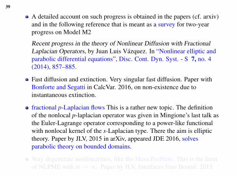
40

Some future Directions

Other nonlocal linear operators (hot topic)

Elliptic theory (main topic, by many authors)

Geostrophic flows (this is more related to Fluid Mechanics)

Reaction-diffusion and blowup

Geometrical flows, fractional Yamabe (MMar Gonzalez, Sire)

Chemotaxis systems, ....

40

Some future Directions

Other nonlocal linear operators (hot topic)

Elliptic theory (main topic, by many authors)

Geostrophic flows (this is more related to Fluid Mechanics)

Reaction-diffusion and blowup

Geometrical flows, fractional Yamabe (MMar Gonzalez, Sire)

Chemotaxis systems, ....

41

Outline




4 Recent team work


42

Operators and Equations in Bounded Domains

Work needs a different lecture. It comes from long time collaborationwith Matteo Bonforte, and recently with Yannick Sire and AlessioFigalli.We develop a new programme for Existence, Uniqueness, Positivity, Apriori bounds and Asymptotic behaviour for fractional porous mediumequations on bounded domains, after examining very carefully the setof suitable concepts of FLO in a bounded domain.But the main issue is how many natural definitions we find of the FLOin a bounded domain.Then we use the “dual” formulation of the problem and the concept ofweak dual solution. In brief, we use the linearity of the operator L to liftthe problem to a problem for the potential function

U(x, t) =

∫Ω

u(y, t)G(x, y)dy

Where G is the elliptic Green function for L.

42

Operators and Equations in Bounded Domains

Work needs a different lecture. It comes from long time collaborationwith Matteo Bonforte, and recently with Yannick Sire and AlessioFigalli.We develop a new programme for Existence, Uniqueness, Positivity, Apriori bounds and Asymptotic behaviour for fractional porous mediumequations on bounded domains, after examining very carefully the setof suitable concepts of FLO in a bounded domain.But the main issue is how many natural definitions we find of the FLOin a bounded domain.Then we use the “dual” formulation of the problem and the concept ofweak dual solution. In brief, we use the linearity of the operator L to liftthe problem to a problem for the potential function

U(x, t) =

∫Ω

u(y, t)G(x, y)dy

Where G is the elliptic Green function for L.

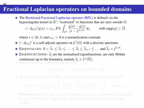
43

Fractional Laplacian operators on bounded domainsThe Restricted Fractional Laplacian operator (RFL) is defined via thehypersingular kernel in Rn, “restricted” to functions that are zero outside Ω.

(−∆|Ω)sg(x) = cN,s P.V.∫RN

g(x)− g(z)|x− z|n+2s dz , with supp(g) ⊂ Ω .

where s ∈ (0, 1) and cn,s > 0 is a normalization constant.

(−∆|Ω)s is a self-adjoint operator on L2(Ω) with a discrete spectrum:

EIGENVALUES: 0 < λ1 ≤ λ2 ≤ . . . ≤ λj ≤ λj+1 ≤ . . . and λj j2s/N .

EIGENFUNCTIONS: φj are the normalized eigenfunctions, are only Holdercontinuous up to the boundary, namely φj ∈ Cs(Ω) .Lateral boundary conditions for the RFL:

u(t, x) = 0 , in (0,∞)×(RN \ Ω

).

The Green function G of RFL satisfies a strong behaviour condition (K4)

G(x, y) 1|x− y|N−2s

(δγ(x)

|x− y|γ ∧ 1)(

δγ(y)

|x− y|γ ∧ 1), with γ = s

References.(K4) Bounds proven by Bogdan, Grzywny, Jakubowski, Kulczycki,Ryznar (1997-2010). Eigenvalues: Blumental-Getoor (1959), Chen-Song(2005).

43

Fractional Laplacian operators on bounded domainsThe Restricted Fractional Laplacian operator (RFL) is defined via thehypersingular kernel in Rn, “restricted” to functions that are zero outside Ω.

(−∆|Ω)sg(x) = cN,s P.V.∫RN

g(x)− g(z)|x− z|n+2s dz , with supp(g) ⊂ Ω .

where s ∈ (0, 1) and cn,s > 0 is a normalization constant.

(−∆|Ω)s is a self-adjoint operator on L2(Ω) with a discrete spectrum:

EIGENVALUES: 0 < λ1 ≤ λ2 ≤ . . . ≤ λj ≤ λj+1 ≤ . . . and λj j2s/N .

EIGENFUNCTIONS: φj are the normalized eigenfunctions, are only Holdercontinuous up to the boundary, namely φj ∈ Cs(Ω) .Lateral boundary conditions for the RFL:

u(t, x) = 0 , in (0,∞)×(RN \ Ω

).

The Green function G of RFL satisfies a strong behaviour condition (K4)

G(x, y) 1|x− y|N−2s

(δγ(x)

|x− y|γ ∧ 1)(

δγ(y)

|x− y|γ ∧ 1), with γ = s

References.(K4) Bounds proven by Bogdan, Grzywny, Jakubowski, Kulczycki,Ryznar (1997-2010). Eigenvalues: Blumental-Getoor (1959), Chen-Song(2005).

44

Fractional Laplacian operators on bounded domains

The The Spectral Fractional Laplacian operator (SFL)

(−∆Ω)sg(x) =∞∑j=1

λsj gj φj(x) =

1Γ(−s)

∫ ∞0

(et∆Ωg(x)− g(x)

) dtt1+s .

where ∆Ω is the classical Dirichlet Laplacian on the domain Ω,

gj =

∫Ω

g(x)φj(x) dx , with ‖φj‖L2(Ω) = 1 .

EIGENVALUES: 0 < λ1 ≤ λ2 ≤ . . . ≤ λj ≤ λj+1 ≤ . . . and λj j2/n.

EIGENFUNCTIONS: φj are as smooth as the boundary of Ω allows,namely when ∂Ω is Ck, then φj ∈ C∞(Ω) ∩ Ck(Ω) for all k ∈ N .

Lateral boundary conditions for the SFL. They are better defined by using theCaffarelli-Silvestre extension adapted to bounded domain as a cylinder. Thenwe put U = 0 on the lateral boundary x ∈ ∂Ω, y > 0.

The Green function of SFL satisfies a stronger assumption

G(x, y) 1|x− y|n−2s

(δγ(x)

|x− y|γ ∧ 1)(

δγ

|x− y|γ ∧ 1), with γ = 1

44



(−∆Ω)sg(x) =∞∑j=1

λsj gj φj(x) =

1Γ(−s)

∫ ∞0


) dtt1+s .


gj =

∫Ω






G(x, y) 1|x− y|n−2s

(δγ(x)

|x− y|γ ∧ 1)(

δγ

|x− y|γ ∧ 1), with γ = 1

44



(−∆Ω)sg(x) =∞∑j=1

λsj gj φj(x) =

1Γ(−s)

∫ ∞0


) dtt1+s .


gj =

∫Ω






G(x, y) 1|x− y|n−2s

(δγ(x)

|x− y|γ ∧ 1)(

δγ

|x− y|γ ∧ 1), with γ = 1

45


Censored Fractional Laplacians (CFL)This is another option that has been introduced in 2003 by Bogdan, Burdzy andChen. Definition

Lf (x) = P.V.∫

Ω

(f (x)− f (y))a(x, y)

|x− y|N+2s dy , with12< s < 1 ,

where a(x, y) is a measurable, symmetric function bounded between twopositive constants, satisfying some further assumptions; for instancea ∈ C1(Ω× Ω).

The Green function G(x, y) satisfies condition K4 , proven by Chen, Kim andSong (2010), in the form

G(x, y) 1|x− y|N−2s

(δγ(x)

|x− y|γ ∧ 1)(

δγ(y))

|x− y|γ ∧ 1), with γ = s− 1

2.

Roughly speaking, s ∈ (0, 1/2] would correspond to Neumann boundaryconditions.

45



Lf (x) = P.V.∫

Ω

(f (x)− f (y))a(x, y)

|x− y|N+2s dy , with12< s < 1 ,



G(x, y) 1|x− y|N−2s

(δγ(x)

|x− y|γ ∧ 1)(

δγ(y))

|x− y|γ ∧ 1), with γ = s− 1

2.


45



Lf (x) = P.V.∫

Ω

(f (x)− f (y))a(x, y)

|x− y|N+2s dy , with12< s < 1 ,



G(x, y) 1|x− y|N−2s

(δγ(x)

|x− y|γ ∧ 1)(

δγ(y))

|x− y|γ ∧ 1), with γ = s− 1

2.


46

We have presented 3 models of Dirichlet fractional Laplacian.Put

[a(x, y) = const

]in the last case. The estimates (K4) show that

they are of course not equivalent.

References. K. Bogdan, K. Burdzy, K., Z.-Q. Chen. Censored stableprocesses. Probab. Theory Relat. Fields (2003).Z.-Q. Chen, P. Kim, R. Song, Two-sided heat kernel estimates forcensored stable-like processes. Probab. Theory Relat. Fields (2010).

Last work announced. M. Bonforte, A. Figalli, J. L. Vazquez. Sharpglobal estimates for local and nonlocal porous medium-type equationsin bounded domains, arXiv:1610.09881.

Last ongoing work.D. Stan, F. del Teso, J. L. Vazquez.Asymptotic behaviour ...., yesterday on the BCAM walls.

46


[a(x, y) = const






46


[a(x, y) = const






46


[a(x, y) = const






46


[a(x, y) = const






46


[a(x, y) = const






47

But let us stop here

Thank you, Gracias,

Eskerrik asko

47


Thank you, Gracias,

Eskerrik asko

47


Thank you, Gracias,

Eskerrik asko

47


Thank you, Gracias,

Eskerrik asko

Documents

Linear and nonlinear diffusion with fractional operators · The fractional Laplacian operator Different formulas for fractional Laplacian operator. We assume that the space variable