NUMERICAL SOLUTION FOR THE TIME SPACE … partial differential equations (FPDEs) is presented. ... approximation of the true solution with less computation. In section 6, the stability

U.P.B. Sci. Bull., Series A, Vol. 78, Iss. 4, 2016 ISSN 1223-7027

NUMERICAL SOLUTION FOR THE TIME–SPACE

FRACTIONAL PARTIAL DIFFERENTIAL EQUATIONS BY

USING THE WAVELET MULTI–SCALE METHOD

H. AMINIKHAH1, M. TAHMASEBI2, M. MOHAMMADI ROOZBAHANI3

In this paper, a practical method for numerical solutions of the time-space

fractional partial differential equations (FPDEs) is presented. The wavelet method

based on multiple resolutions is used to solve the FPDE. This method transforms the

given FPDE and the boundary conditions to matrix equations with unknown wavelet

coefficients which can be solved by a sequential evaluation of two systems, with

significantly less computational effort. Theoretical considerations are discussed. For

illustration the accuracy and efficiently of the method some numerical examples are

presented

Keywords: Fractional diffusion equation; Wavelet numerical method; Multi

resolutions Method; Fractional differential equations.

1. Introduction

There is a vast literature on efficient methods for fractional partial

differential equations. These equations are important as they arise naturally in

many applied areas [1-4, 8, 11, 15, 17, 18-20]. Almost all methods of solving

FPDEs are the generalizations of the same strategies for the solutions of PDEs.

Multiscale wavelet method for the solution of PDEs are used in many works [6,

10, 14, 16, 22]. Also Mclaren et. al. handled multiscaling collocation method in

different way [13]. Their method keeps the different levels of resolution consistent

with each other which has a property similar to domain decomposition methods.

In the present work, we are interested to combine Adams fractional and the

multiscale techniques to solve the fractional partial differential equations

efficiently. The main objective of the present work is to extended the multiscaling

collocation method in [13] for FPDE. We intend to consider a kind of

“generalized diffusion” equation which is referred to the space-time FDE with

Robin condition boundary,

1Department of Applied Mathematics, School of Mathematical Sciences, University of

Guilan, P.O. Box 41938-1914, Rasht, Iran, e-mail: [email protected] 2Department of Applied Mathematics, Faculty of Mathematical Sciences, Tarbiat Modares

University, P.O. Box 14115-134 ,Tehran, Iran, e-mail: [email protected] 3Department of Applied Mathematics, School of Mathematical Sciences, University of

Guilan, P.O. Box 41938-1914, Rasht, Iran, e-mail: [email protected]

mailto:[email protected]



H. Aminikhah, M. Tahmasebi, M. Mohammadi Roozbahani 176

1 2 3

4 5 6

, , , 0, , 0 , 0 1,

,0 ,

0, 0, ,

, , ,

t

x

x

D u x t Lu x t x n t T

u x g x

c u t c u t c

c u n t c u n t c

(1)

where 0

. k

N

k x

k

L f D

, and kf x are sufficiently well behaved functions on and

the operator xD is Caputo fractional derivative of order defined by [15]

1

1

0

1,

1

x mm

x mD F x x F d

m

(2)

where 1m m , m .

In this approach, we utilize cubic B-spline wavelets which are symmetric,

compactly supported and smooth enough. The paper is organized as follows:

In section 2 the basic definitions and required properties of the wavelets

are briefly mentioned. In section 3 the fractional derivative matrix was

approximated by collocation method. In section 4 the wavelets and scaling

functions were reshaped to satisfy the boundary conditions exactly. In section 5

we employ the fractional Adams method for time discretization FPDE, then by the

operational matrices we convert the FPDE to a linear system. Finally, by multi-

resolution method in some subdomains this system divides to some smaller

systems which each of them has different resolution and less computation than the

primary system, then by combining the solutions of these systems, we derive an

approximation of the true solution with less computation. In section 6, the stability

of the method is investigated. In section 7 numerical examples are given to

demonstrate the validity of the proposed method.

2. Wavelet analysis Preliminaries and notations

In this section, we present some notations, definitions and preliminary

facts of the wavelet theory which will be used further in this work. The discrete

wavelets constitute a family of functions constructed from dilation and translation

of a function called the mother wavelet x . They are defined by

2

, 2 2 .j

j

j k x x k

(3)

The best way to understand wavelets is through a multi-resolution analysis [5].

Given a function 2f x L , a multi-resolution analysis (MRA) of 2L

produces a sequence of subspaces 0 1j jV V V such that the projections

of f onto these spaces give finer approximations of the function f as j .

There exists 0V such that x k , k is a Riesz basis in 0V . The function

is called the scaling function. As a consequence of above definition, jV is spanned

Numerical solution for the time-space FPDEs by using the wavelet multi-scale method 177

by 2, 2 2

jj

j k x x k

. One may construct wavelets by first completing the

spaces jV to the space 1jV by the space jW , i.e., 1j j jV V W . In such away there

exists a function such that jW is spanned by 2 j x k . The space jW include

all the functions in 1jV that are orthogonal to all those in jV under 2L -inner

product. The set of functions which form a basis for the space jW are called

wavelets [3, 4]. For the inclusion 0 1V V and 0 1W V there are two important

identities:

2 2 , 2 2 .k k

k k

t h t k t g t k (4)

For more details, refer to [5].

Definition (Biorthogonal wavelets): Two functions 2, L are

called biorthogonal wavelets if each of the sets : ,jk j k and : ,jk j k be

a Riesz basis of 2L and they are biorthogonal to each other in the following

sense

, , , ,,j k l m j l k m for all , , ,j k l m .

Designing biorthogonal wavelets allows more freedom than orthogonal wavelets.

One of them is the possibility of constructing symmetric wavelet functions. Since

they define a multi-resolution analysis, the dual functions must satisfy

2k

k

x h x k and 2 .k

k

x g x k (5)

In this work we will use biorthogonal wavelets whose scaling functions are the

cubic B-splines:

4

3

3

0

411 ,

6

k

k

x B x x kk

(6)

where 0,

0 0.

n

n x xx

x

The fractional derivative of cubic B-spline 3B x is given in [11]:

4

3

3

0

411 .

4

k

x

k

D B x x kk

(7)

2.1. Fast Wavelet Transform (FWT)

From 1j j jV V W , every function 1 1j jv V can be written uniquely as

the sum of a function j jv V and a function j jw W . Then there exist some

coefficients such that

1

1, 1, , , , ,

,

.

j j j

j k j k j k j k j k j k

k k k

v v x w x

a x a x b x

(8)

http://en.wikipedia.org/wiki/Orthogonal_wavelet


In other words, we have two representations of the function 1jv , one as an

element in 1jV and associated with the sequence 1,j ka , and another as a sum of

elements in jV and jW associated with the sequences ,j ka and ,j kb . The

following relations show how to pass between these representations. From (5) and

(8) and biorthogonal property of wavelets,

, 1,2 ,j k i j k i

i

a h a (9)

and

, 1,2 .j k i j k i

i

b g a (10)

These formulas define the FWT, let 1ja , ja and jb be vectors which contain

coefficients 1,j ka , ,j ka and ,j kb respectively, then the FWT maps the vector

1ja onto vectors ja and jb :

1 .j

j

j

aFWT a

b

For numerical purposes we have to reverse the process to define Inverse fast

wavelet transform (IFWT). To do this, taking the inner product of each side of (8)

with 1,j k , we derive

1, 2 , 2 , ,j k k n j n k l j l

n l

a h a g b (11)

so we can define IFWT as following:

1 .j

j

j

aIFWT a

b

3. Matrix approximations

In this work we need operational matrix M to approximate xD on jV

where 0 1 . We will use a collocation based method to calculate them. First

we want to approximate any function of 2L as finite series of wavelets and

scaling functions. For a fixed 0j , we use jV as a basic space, we add extra

spaces jW for increasing the resolution. Let jV

f denote the projection 2f L

onto jV . From 1j j jV V W we have

1

1 2 1

, , 1 1,

1 1 1

,j

N N N

j i j i j i j i j i j iVi i i

f x b x a x a x

(12)


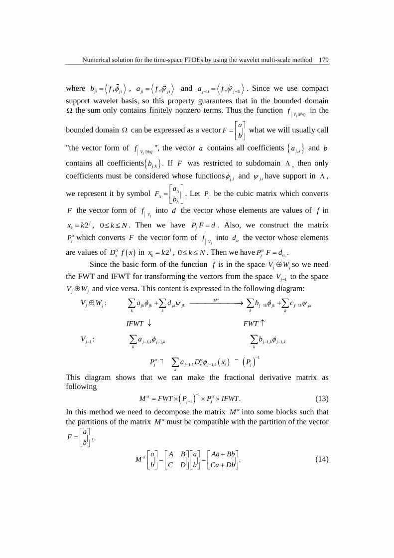
where ,ji j ib f , ,ji j ia f and 1 1,j i j ia f . Since we use compact

support wavelet basis, so this property guarantees that in the bounded domain

the sum only contains finitely nonzero terms. Thus the function jV Wj

f

in the

bounded domain can be expressed as a vectora

Fb

what we will usually call

"the vector form of jV Wj

f

", the vector a contains all coefficients ,j ka and b

contains all coefficients ,j kb . If F was restricted to subdomain , then only

coefficients must be considered whose functions ,j i and .j i have support in ,

we represent it by symbol a

Fb

. Let jP be the cubic matrix which converts

F the vector form of

jVf into d the vector whose elements are values of f in

2 j

kx k , 0 k N . Then we have jP F d . Also, we construct the matrix

jP which converts F the vector form of jV

f into d the vector whose elements

are values of xD f x in 2 j

kx k , 0 k N . Then we have jP F d

.

Since the basic form of the function f is in the space j jV W so we need

the FWT and IFWT for transforming the vectors from the space 1jV to the space

j jV W and vice versa. This content is expressed in the following diagram:

1 1

1 1, 1, 1, 1,

1

1, 1,

:

:

M

j j jk jk jk jk j k jk j k jk

k k k k

j j k j k j k j k

k k

j j k x j k i j

k

V W a d b c

IFWT FWT

V a b

P a D x P

This diagram shows that we can make the fractional derivative matrix as

following

1

1 .j jM FWT P P IFWT

(13)

In this method we need to decompose the matrix M into some blocks such that

the partitions of the matrix M must be compatible with the partition of the vector

aF

b

,

.a A B a Aa Bb

Mb C D b Ca Db

(14)


In addition, if we use the restricted vector a

Fb

, then the matrix M must be

adapted with the size of F , we denote by M

.

.a A B a A a B b

Mb C D b C a D b

(15)

3.1. Advection matrix

One further requirement is the multiplication by the space independent

function g x . We create the linear operator G to approximate the multiplication.

1

,j jFWT P G P IFWT

(16)

G is a diagonal matrix with the values of function g in 2 j

kx k , 0 k N .

In the general case, we can represent the operator . k

k x

k

L f D

in the

following matrix form.

1 1

1

,

k

k

j k j j j

k

j k j

k

M FWT P F P IFWT FWT P P IFWT

FWT P F P IFWT

(17)

where kF is a diagonal matrix with the values of function kf in some locations.

4. Boundary conditions

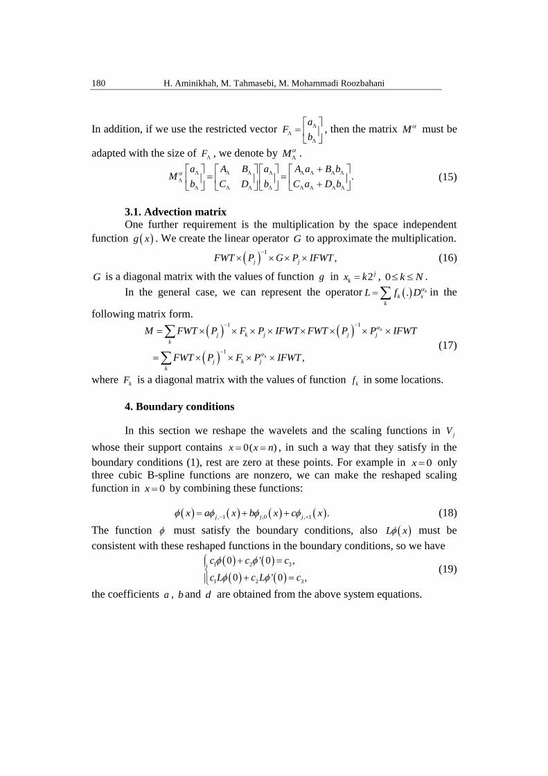
In this section we reshape the wavelets and the scaling functions in jV

whose their support contains 0( )x x n , in such a way that they satisfy in the

boundary conditions (1), rest are zero at these points. For example in 0x only

three cubic B-spline functions are nonzero, we can make the reshaped scaling

function in 0x by combining these functions:

, 1 ,0 , 1 .j j jx a x b x c x (18)

The function must satisfy the boundary conditions, also L x must be

consistent with these reshaped functions in the boundary conditions, so we have

1 2 3

1 2 3

0 ' 0 ,

0 ' 0 ,

c c c

c L c L c

(19)

the coefficients a , b and d are obtained from the above system equations.


5. The proposed method

We consider the fractional Adams method for solving FPDE (1), This

method was first studied by Diethelm, Ford and Freed [7]. Their method for

solving equation (20) is as follows:

,D y t f t y t , 00y y , 0 1, (20)

1 0 , 1 1, 1 1 1

0

, , ,2

n

n k n k k n n n n

k

hy y c f t y c f t y

(21)

where

1

1 1 1

, 1

1 , 0,

2 2 1 , 1 ,

1, 1.k n

n n n k

c n k n k n k k n

k n

(22)

and , : 0,1,.., , .k k k

Th t kh k N y y t

N

Let nu denote the exact solution ., nu t and nu denote approximation

solution of it. So approximation solution for the time space-fractional diffusion

equation (1) by using the fractional Adam's method would be

1 0 , 1 1

0

.2

n

n k n k n

k

hu u c Lu Lu

(23)

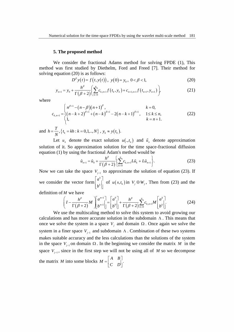
Now we can take the space 1jV to approximate the solution of equation (23). If

we consider the vector formk

k

a

b

of , ku x t in j jV W , Then from (23) and the

definition of M we have

1 0

, 11 00

.2 2

n kn

k nn kk

a a ah hI M c M

b b b

(24)

We use the multiscaling method to solve this system to avoid growing our

calculations and has more accurate solution in the subdomain . This means that

once we solve the system in a space jV and domain . Once again we solve the

system in a finer space 1jV and subdomain . Combination of these two systems

makes suitable accuracy and the less calculations than the solutions of the system

in the space 1jV on domain . In the beginning we consider the matrix M in the

space 1jV , since in the first step we will not be using all of M so we decompose

the matrix M into some blocks .A B

MC D


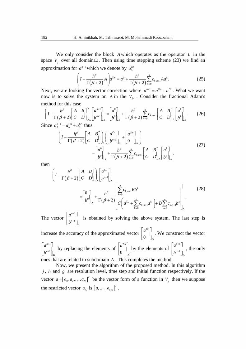
We only consider the block A which operates as the operator L in the

space jV over all domain . Then using time stepping scheme (23) we find an

approximation for 1na which we denote by Tma

0

, 1

0

.2 2

nTm k

k n

k

h hI A a a c Aa

(25)

Next, we are looking for vector correction where 1n Tm Cra a a . What we want

now is to solve the system on in the 1jV . Consider the fractional Adam's

method for this case

1 0

, 11 00

.2 2

n kn

k nn kk

A B a a A B ah hI c

C D C Db b b

(26)

Since 1n Tm Cra a a

thus

1

0

, 100

2 0

,2

Cr Tm

n

kn

k n kk

A B a ahI

C D b

a A B ahc

C Db b

(27)

then

1

, 1

0

0

, 1 , 1

0 0

2

0.

2

r

m

C

n

nk

k n

k

n nT k k

k n k n

k k

A B ahI

C D b

c Bbh

bC a c a D c b

(28)

The vector

1

1

n

n

a

b

is obtained by solving the above system. The last step is

increase the accuracy of the approximated vector 0

Tma

. We construct the vector

1

1

n

n

a

b

by replacing the elements of 0

Tma

by the elements of 1

1

n

n

a

b

, the only

ones that are related to subdomain . This completes the method.

Now, we present the algorithm of the proposed method. In this algorithm

j , h and g are resolution level, time step and initial function respectively. If the

vector 0 2, , ,T

Na a a a be the vector form of a function in jV then we suppose

the restricted vector a is 1, ,T

r sa a .


5.1. Algorithm:

1. 0 1 2, , , Nv g g g where 2 jN m and 2 0, ,2j

kg g k k N

2. 1

j

aFWT P v

b

3. Constructing matrix M by using (17)

4. Blocking the matrix A B

MC D

where 1: 1,1: 1A M N N ,

1: 1, 1: 2 1B M N N N and so on for C and D

5. A B

MC D

Limiting M to subdomain , where

: 1, : 1A A r s r s , : 1, :B B r s r s and so on for C and D

6. For 0n to k do

7. n

n

a a

b b

8. : 1a a r s , :b b r s

9. Solve the system (25) to get vector Tma

10. : 1Tm Tma a r s

11. Solve the system (28) to get vector Cra

b

12. Cr Tma a a ,

13. : 1Tma r s a , :b r s b , Tma

vb

14. End for

6. Stability

In order to show stability of the approximate solution, we recall discrete

Gronwall lemma.

Lemma (Discrete Gronwall Lemma): If ky , kf , and kg are nonnegative

sequences and

0

0,n n k k

k n

y f g y for n

(29)

then

0

exp 0.n n k k i

k n k i n

y f f g g for n

(30)

If, in addition, kf is nondecreasing then


0

exp 0.n n i

i n

y f g for n

(31)

Now, let nu denote the approximation solution of equation (23), and nU be the

vector form of nu in the jV and 0 1, , , , , ,T

n n n N nU u x t u x t u x t where

2 j

kx k , 0 k N . Since n njP U U , from equation (23) we have

1 1 1 1

1 0 1, 1

0

.2

n

n k nj j k n j j

k

hP U P U c MP U MP U

(32)

Choosing h small enough that

11

2 2

hM

guarantees nonsingularity of

the matrix 2

hI M

, then

1

12

21

2

hI M

hM

,

therefore, we have

1

11 0

1

1

, 1

0

2

.2 2

n j j

n

kj j k n

k

hU P I M P U

h hP I M P M c U

(33)

Since

1

22

hI M

and T

hN

, we have

1 1

1 0 , 1

0

2

2 .2

n

n kj j j j k n

k

T

NU P P U P P M c U

(34)

By applying Gronwall's inequality, we obtain

, 1

1 01 2

0

exp ,n

k nn

k

cU C U C T

N

(35)

since

1 1 1

, 1 2 1 22

k nc n k n k n k

N N N N N

is bounded and

increasing function with respect to so we have

1 01 2exp 2 ,nU C U C T (36)


where 1

1 2 j jC P P and

1

2

4

2j j

hC P P M

, this completes the proof of

stability.

7. Numerical Examples

Example 7.1. We consider the following time space fractional differential

equation

, , ,t tD u x t D u x t

the initial condition and the boundary conditions are as follows:

2

1exp , 3 4,

1, 20, 0,0 2, ,0 1 2

0, .

xu t u t t u x x

otherwise

For comparison, the example 1 was solved numerically in different levels of

resolutions. Table 1 shows the convergence when j decreases, also the Figure 1

shows in different times the approximated results satisfy the boundary conditions

exactly. Table 1. The errors are the difference between the jV results and The 1jV results ( 1/j jV V )

with h=0.01 at t=0.5.

0.9

x 3 4/V V 4 5/V V 5 6/V V 6 7/V V 7 8/V V solution on 8V

1.5 0.0030298 -0.000261 -6.163E-6 -3.025E-7 -1.516E-8 3.5574E-7

2 0.0007083 7.9038E-6 8.4961E-7 9.6163E-8 1.0941E-8 0.11612065

2.5 0.000198 -9.662E-6 1.9387E-9 -1.41E-9 7.848E-11 0.28671766

3 0.000521 -1.194E-5 -3.205E-7 -1.114E-8 4.754E-10 0.29474804

3.5 -0.000733 -0.000135 -1.081E-5 -8.237E-7 -6.865E-8 0.10448197

0.7

x 3 4/V V 4 5/V V 5 6/V V 6 7/V V 7 8/V V solution on 8V

1.5 -3.29E-6 -2.831E-7 -1.968E-9 -6.91E-11 8.928E-12 2.3211E-9

2 0.0002645 1.4228E-6 -2.444E-7 -6.756E-9 -7.375E-10 0.00223121

2.5 0.0002652 3.0337E-6 -2.905E-7 -2.917E-9 -2.156E-10 0.03290537

3 0.0002006 3.0142E-6 -1.995E-7 -1.829E-10 1.453E-10 0.08704351

3.5 0.0001583 3.6176E-6 3.9999E-9 1.5924E-8 2.7148E-9 0.12114837


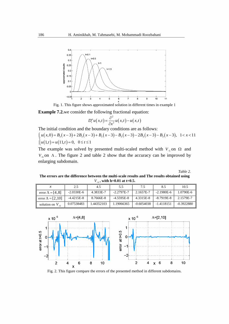
Fig. 1. This figure shows approximated solution in different times in example 1

Example 7.2.we consider the following fractional equation:

2

2, , ,tD u x t u x t u x t

x

The initial condition and the boundary conditions are as follows:

3 3 3 3 3 3,0 3 2 3 3 3 2 3 3 , 1 11

1, 11, 0, 0 1

u x B x B x B x B x B x B x x

u t u t t

The example was solved by presented multi-scaled method with 5V on and

6V on . The figure 2 and table 2 show that the accuracy can be improved by

enlarging subdomain.

Table 2.

The errors are the difference between the multi-scale results and The results obtained using

6V , with h=0.01 at t=0.5.

x 2.5 4.5 5.5 7.5 8.5 10.5

error [4,8] -2.0330E-6 4.3833E-7 -2.2797E-7 2.1657E-7 -2.1980E-6 1.0790E-6

error [2,10] -4.4215E-8 8.7666E-8 -4.5595E-8 4.3315E-8 -8.7919E-8 2.1579E-7

solution on 6V 0.07538483 1.44352103 1.19066365 -0.6054038 -1.4118151 -0.3922880

Fig. 2. This figure compare the errors of the presented method in different subdomains.


8. Conclusions

In this work a practical approach for solving time space fractional partial

differential equation is presented. Multi scaling method via wavelets is used to

increase resolution in some locations, furthermore the computations are reduced

because of the compact support of wavelets, and also wavelets are employed in

such a way that they satisfy the boundary conditions exactly. The method can be

extended to nonlinear FPDEs that is now under progress.

Acknowledgement

We are very grateful to two anonymous referees for their careful reading

and valuable comments which led to the improvement of this paper. We would

like to thank Dr. Donald A. McLaren for his useful comments.

R E F E R E N C E S

[1] B. Baeumer, M. M. Meerschaert, D. A. Benson and S. W. Wheatcraft, ‘‘Subordinated

advection–dispersion equation for contaminant transport’’, Water Resour. Res., Vol. 37, no.

6, 2001, pp. 1543–1550. [2] D. Benson, R. Schumer, M. Meerschaert and S. Wheatcraft, ‘‘Fractional dispersion, Levy

motions and the MADE tracer tests’’, Transport Porous Media, Vol. 42, no. 1, 2001, pp. 211–

240. [3] D. Benson, S. Wheatcraft and M. Meerschaert, ‘‘Application of a fractional advection–

dispersion equation’’, Water Resour. Res., Vol. 36, no. 6, 2000, pp. 1403–1412. [4] D. Benson, S. Wheatcraft and M. Meerschaert, ‘‘The fractional-order governing equation of

Levy motion’’, Water Resour. Res., Vol. 36, no. 6, 2000, pp. 1413–1424. [5] C. Blatter, ‘‘Wavelets, A Primer’’, A K Peters/CRC Press, 2002. [6] W. Dahmen, A. Kurdila and P. Oswald, ‘‘Multiscale Wavelet Methods for Partial Differential

Equations’’, Academic Press, Toronto, 1997. [7] K. Diethelm, N.J. Ford and A.D. Freed, ‘‘Detailed error analysis for a fractional Adams

method’’, Numer. Algorithms, Vol. 36, no. 1, 2004, pp. 31–52. [8] R. Gorenflo, F. Mainardi, E. Scalas and M. Raberto, ‘‘Fractional calculus and continuous-

time finance III, The diffusion limit, Mathematical finance (Konstanz, 2000)’’, Trends in

Math., Birkhuser, Basel, 2001, pp. 171–180. [9] J.C. Goswami and Andrew K. Chan, ‘‘Fundamentals of Wavelets. Theory, Algorithms and

Applications’’, John Wiley and Sons, New York, 1999. [10] J. S. Hesthaven and L. M. Jameson, ‘‘A Wavelet optimized adaptive multi-domain method’’,

Journal of Computational Physics, Vol. 145, no. 1, 1998, pp. 280-296. [11] X. Li, ‘‘Numerical solution of fractional equations using cubic b-spline wavelet collocation

method’’, Commun. Nonlinear Sci. Numer. Simulat., Vol. 17, no. 10, 2012, pp. 3934-3946. [12] S. Mallat, ‘‘A Wavelet Tour of Signal Processing’’, Academic Press, New York, 1999. [13] D. A. McLaren, ‘‘Sequential and localized implicit wavelet-based solvers for stiff partial

differential equations’’, Ph.D. Thesis, 2012. [14] M. Mehra and N.K.-R. Kevlahan, ‘‘An adaptive multilevel wavelet solver for elliptic

equations on an optimal spherical geodesic grid’’, SIAM J. Sci. Comput., Vol. 30, no. 6,

2008, pp. 3073–3086. [15] K.S. Miller and B. Ross, ‘‘An Introduction to the Fractional Calculus and Fractional

Differential Equations’’, John Wiley and Sons, New York, 1993.


[16] S. Muller and Y. Stiriba, ‘‘A multilevel finite volume method with multiscale-based grid

adaptation for steady compressible flows’’, J. Comput. Appl. Math., Vol. 277, no. 2, 2009,

pp. 223–233. [17] I. Podlubny, ‘‘Fractional Differential Equations’’, Academic Press, SanDiego, CA, 1999. [18] M. Raberto, E. Scalas and F.Mainardi, ‘‘Waiting-times and returns in high-frequency

5nancial data: an empirical study’’, Physica A, Vol. 314, no. 1, 2002, pp. 749–755. [19] L. Sabatelli, S. Keating, J. Dudley and P. Richmond, ‘‘Waiting time distributions in 5nancial

markets’’, The European Physical Journal B, Vol. 27, no. 2, 2002, pp. 273–275. [20] R. Schumer, D.A. Benson, M.M. Meerschaert and B. Baeumer, ‘‘Multiscaling fractional

advection–dispersion equations and their solutions’’, Water Resour. Res., Vol. 39, no. 1,

2003, pp. 1022–1032. [21] W. Sweldens, ‘‘The Construction and Application of Wavelets in Numerical Analysis’’,

Ph.D. Thesis, Leuven, 1995. [22] O.V. Vasilyev and S. Paolucci, ‘‘A dynamically adaptive multilevel wavelet collocation

method for solving partial differential equations in a finite domain’’, J. Comput. Phys., Vol.

125, no. 2, 1996, pp. 498–512.

Documents

NUMERICAL SOLUTION FOR THE TIME SPACE … partial differential equations (FPDEs) is presented. ... approximation of the true solution with less computation. In section 6, the stability