A Predictor-Corrector Approach for the

Numerical Solution of Fractional Differential

Equations

Kai Diethelm* Neville J. Ford t Alan D. Freed t

December 19, 2001

Abstract

We discuss an Adams-type predictor-corrector method for the numer-

ical solution of fractional differential equations. The method may be usedboth for linear and for nonlinear problems, and it may be extended tomulti-term equations (involving more than one differential operator) too.

1 Statement of the Problem

In this paper we want to discuss an algorithm for the numerical solution of dif-ferential equations of fractional order, equipped with suitable initial conditions.

To be precise, we first look at the fractional differential equation

D_.V(x)=/(z, v(x)), (1)

where a > 0 (but not necessarily c_ E N). We shall determine a solution of this

equation on the interval [0, T], say, where T is a suitable positive number. At a

later stage we will also investigate a more general problem (see §4) but for themoment we restrict ourselves to (1) in order to explain the fundamental ideas

behind our strategy.

It is well known [4, 31, 33] that there are many ways to define a fractionaldifferential operator. The special operator D. _ that we are using in (1) is defined

by

D.ay(x) = ..]'rn-ay(m)(X) (2)

"Institut fiir Angewandte Mathematik, Technische Universitgt Braunschweig, Pockels-str. 14, 38106 Braunschweig, Germany (K. Diethelm©tu-bs .de).

tDepartment of Mathematics, Chester College, Parkgate Road, Chester CH1 4BJ, UnitedKingdom (nj :ford©chester. ac. uk)

tPolymers Branch, MS 49-3, NASA's John H. Glenn Research Center at Lewis Field, 21000Brookpark Road, Cleveland, OH 44135, USA (Alan. D.Freed©grc. nasa. gov).

This report is a preprint of an article submitted to a journal forpublication. Because of changes that may be made before formal

publication, this preprint is made available with the understandingthat it will not be cited or reproduced without the permission of theauthor.

https://ntrs.nasa.gov/search.jsp?R=20020024453 2018-07-13T13:20:41+00:00Z

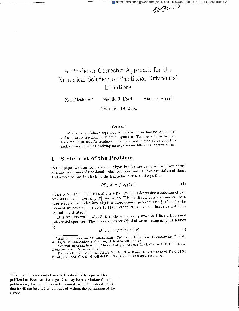
wherem := [c_1 is just the value a rounded up to the nearest integer, y('_) is

the ordinary ruth derivative of y (recall that m is an integer, so we are dealing

with the classical situation), and

/0•1 (x - t)_-lz(t)dt (3)J_z(x)- r(9)

is the Riemann-Liouville integral operator of order/3 > 0. It is common practice

to call the operator D. _ the Caputo differential operator of order c_ because it.

has apparently first been used for the solution of practical problems by Caputo

[5]. Note however that, according to [4, p. 11], it had already been introducedin a 19th century paper of Liouville.

A typical feature of differential equations (classical or fractional) is that one

needs to specify additional conditions to make sure that the solution is unique.

In many situations these additional conditions describe certain properties of the

solution at the beginning of the process, i.e. at the point x = 0. Therefore such

a problem is called an initial value problem. It is easily seen that the number ofinitial conditions that one needs to specify in order to obtain a unique solution

is m = rc_]. In particular, if 0 < c_ < 1 (which is the case in many applications),we have to specify just one condition. However the precise form of this condition

is not arbitrary. Rather, when fractional differential equations are concerned, itturns out that there is a close connection between the type of the initial condition

and the type of the fractional derivative. This is actually also the reason for us

to choose the Caputo derivative and not the Riemann-Liouville derivative that is

more commonly used in pure mathematics: For the Riemann-Liouville case, one

would have to specify the values of certain fractional derivatives (and integrals)of the unknown solution at the initial point x = 0, cf. [33, §42]. However, when

we are dealing with a concrete physical application then the unknown quantity

y will typically have a certain physical meaning (e.g. a dislocation), but it isnot clear what the physical meaning of a fractional derivative of y is, and hence

it is also not clear how such a quantity can be measured. In other words,

the required data simply will not be available in practice. V_rhen we deal with

Caputo derivatives however, the situation is different. We may [11] specify the

initial values y(0), y'(0),..., y(-_-ll (0), i.e. the function value itself and integer-order derivatives. These data typically have a well understood physical meaning

and can be measured.

Note that Lorenzo and Hartley [27] have discussed the problem of finding thecorrect form of the initial conditions in a more general setting (not necessarily

assuming that the entire history of the process can be observed).Thus we combine our fractional differential equation (1) with initial condi-

tions

y(k)(0) = y_k), k = 0, 1,...,m - 1, (4)

where once again m = [a_ and the real numbers y(ok), k = 0, 1,..., m - 1, are

assumed to be given. It then turns out that, under some very weak conditions

on the function f on the right-hand side of the differential equation, we indeed

can say that a solution exists and that this solution is uniquely determined [11].

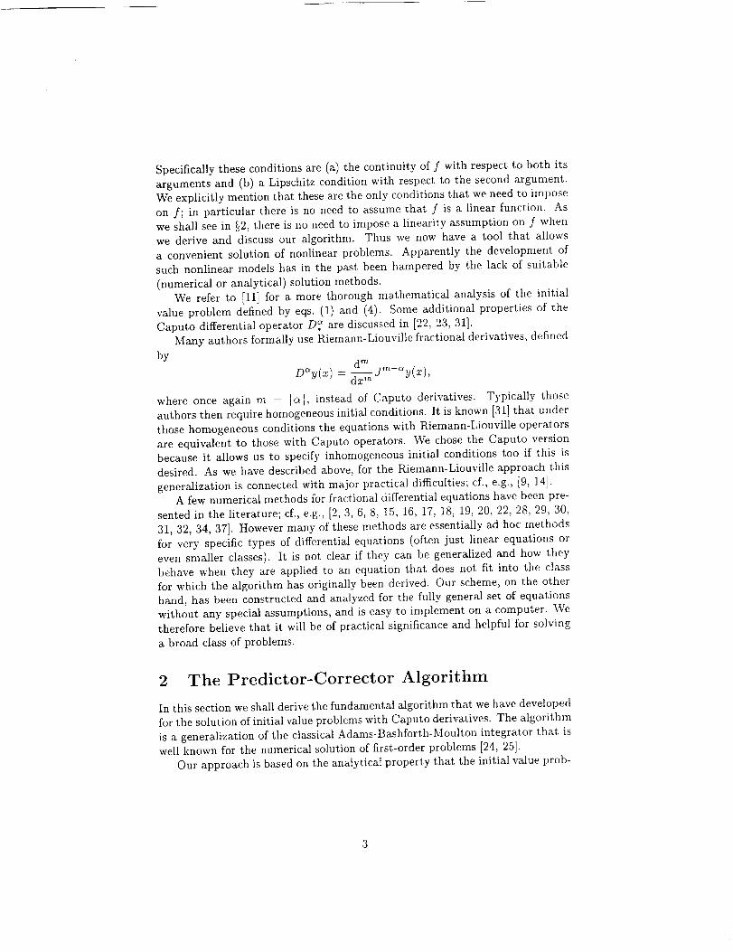
Specificallytheseconditionsare(a)thecontinuityof f with respect to both its

arguments and (b) a Lipschitz condition with respect to the second argument.

We explicitly mention that these are the only conditions that we need to imposeon f; in particular there is no need to assume that f is a linear function. As

we shall see in §2, there is no need to impose a linearity assumption on f when

we derive and discuss our algorithm. Thus we now have a tool that allows

a convenient solution of nonlinear problems. Apparently the development of

such nonlinear models has in the past been hampered by the lack of suitable

(numerical or analytical) solution methods.

We refer to [11] for a more thorough mathematical analysis of the initial

value problem defined by eqs. (1) and (4). Some additional properties of the

Caputo differential operator D. _ are discussed in [22, 23, 3:1].Many authors formally use Riemann-Liouville fractional derivatives, defined

by

where once again rn = [c_], instead of Caputo derivatives. Typically those

authors then require homogeneous initial conditions. It is known I31] that underthose homogeneous conditions the equations with Riemann-Liouville operators

are equivalent to those with Caputo operators. We chose the Caputo version

because it allows us to specify inhomogeneous initial conditions too if this is

desired. As we have described above, for the Riemann-Liouville approach this

generalization is connected with major practical difficulties; cf., e.g., [9, 14].A few numerical methods for fractional differential equations have been pre-

sented in the literature; cf., e.g., [2, 3, 6, 8, 15, 16, 17, :18, 19, 20, 22, 28, 29, 30,

3:1, 32, 34, 37]. However many of these methods are essentially ad hoc methods

for very specific types of differential equations (often just linear equations or

even smaller classes). It is not clear if they can be generalized and how they

behave when they are applied to an equation that does not fit into the classfor which the algorithm has originally been derived. Our scheme, on the other

hand, has been constructed and analyzed for the fully general set of equationswithout any special assumptions, and is easy to implement on a computer. We

therefore believe that it will be of practical significance and helpful for solvinga broad class of problems.

2 The Predictor-Corrector Algorithm

In this section we shall derive the fundamental algorithm that. we have developed

for the solution of initial value problems with Caputo derivatives. The algorithmis a generalization of the classical Adams-Bashforth-Moulton integrator that is

well known for the numerical solution of first-order problems [24, 25].Our approach is based on the analytical property that the initial value prob-

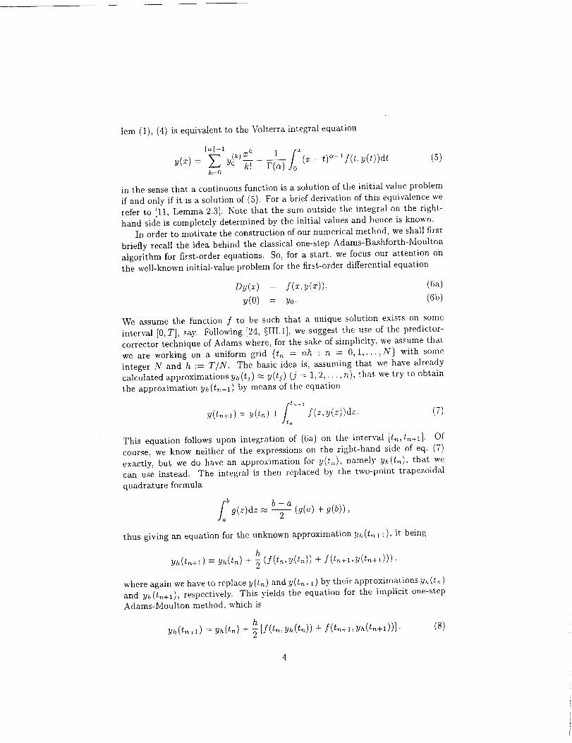
lem(1),(4)isequivalentto theVolterraintegralequation

y(x)= E y;klz kk_(.+-_1 fo (x-t)_-lf(t'y(t))dt (5)k=0

in the sense that a continuous function is a solution of the initial value problem

if and only if it is a solution of (5). For a brief derivation of this equivalence we

refer to [11, Lemma 2.3]. Note that the sum outside the integral on the right-

hand side is completely determined by the initial values and hence is known.In order to motivate the construction of our numerical method, we shall first

briefly recall the idea behind the classical one-step Adams-Bashforth-Moulton

algorithm for first-order equations. So, for a start, we focus our attention on

the well-known initial-value problem for the first-order differential equation

Dr(z) = f(_,_(x)), (6a)

y(0) = Y0. (6b)

_re assume the function f to be such that a unique solution exists on some

interval [0, T], say. Following [24, §III.1], we suggest the use of the predictor-

corrector technique of Adams where, for the sake of simplicity, we assume that

we are working on a uniform grid {tn = nh : n = 0,1,...,N} with some

integer N and h := T/N. The basic idea is, assuming that we have already

calculated approximations yh(tj) "_ y(tj) (j = 1, 2,..., n), that we try to obtainthe approximation yh(tn+l) by means of the equation

t_,+ly(t,_+l) = y(t,_) + f(z,y(z))dz. (7)J t_

This equation follows upon integration of (6a) on the interval [tn, t,_+l]. Of

course, we know neither of the expressions on the right-hand side of eq. (7)

exactly, but we do have an approximation for y(t_,), namely yh(t,_), that wecan use instead. The integral is then replaced by the two-point trapezoidal

quadrature formula

Lb b - a9(z)dz _, --7- (9(a) + 9(b)),

thus giving an equation for the unknown approximation yh(t,,+l), it being

hw(t,_+l) = yh(t_) + _ (f(t,_,y(t_)) + f(t,,+l,y(t,,+l))),

where again we have to replace y(t,_) and y(t,_+l) by their approximations yh(t_)

and yn(t,,+l), respectively. This yields the equation for the implicit one-stepAdams-Moulton method, which is

h

yh(tn+l) = yh(t,) + -{ [f(t,, yh(tn)) + f(t,_+,, Yn(t_+l))]. (8)

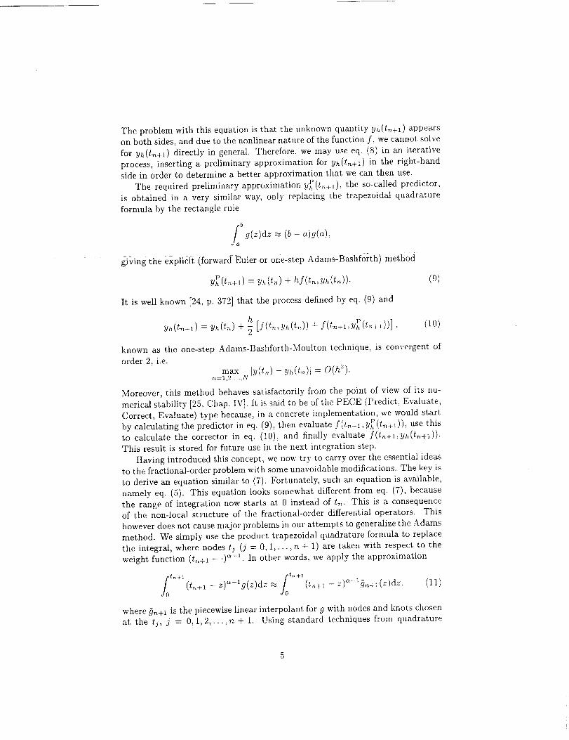
Theproblemwiththisequationisthat theunknownquantityyh(t,_+1) appearson both sides, and due to the nonlinear nature of the function f, we cannot solve

for yh(t,_+l) directly in general. Therefore, we may use eq. (8) in an iterative

process, inserting a preliminary approximation for Yh(t,_+_) in the right-hand

side in order to determine a better approximation that we can then use.

The required preliminary approximation yP(t,_+l), the so-called predictor,h

is obtained in a very similar way, only replacing the trapezoidal quadrature

formula by the rectangle rule

b

giving the explicit (forward Euler or one-step Adams-Bashf0rth) method

yP(t,_+l) = yh(tn) + hf(t,_, yh(t,_)). (9)

It is well known [24, p. 372] that the process defined by eq. (9) and

hyh(t_+l) = yh(t,_) + _ [f(t_,yh_(t,_)) + f(t,_+l,y_(t,_l))], (10)

known as the one-step Adams-Bashforth-Moulton technique, is convergent of

order 2, i.e.

max ly(t_) - _r,(t_)l = O(h2).n=] ,2,...,N

Moreover, this method behaves satisfactorily from the point of view of its nu-

merical stability [25, Chap. IV]. It is said to be of the PECE (Predict, Evaluate,

Correct, Evaluate) type because, in a concrete implementation, we would start

by calculating the predictor in eq. (9), then evaluate f(t,_+l, yPh(t,+l)), use thisto calculate the corrector in eq. (10), and finally evaluate f(t_+_,yj,(t,+_)).

This result is stored for future use in the next integration step.

Having introduced this concept, we now try to carry over the essential ideas

to the fractional-order problem with some unavoidable modifications. The key is

to derive an equation similar to (7). Fortunately, such an equation is available,

namely eq. (5). This equation looks somewhat different from eq. (7), because

the range of integration now starts at 0 instead of t_. This is a consequenceof the non-local structure of the fractional-order differential operators. This

however does not cause major problems in our attempts to generalize the Adams

method. We simply use the product trapezoidal quadrature formula to replace

the integral, where nodes tj (j = 0, 1,...,n + 1) are taken with respect to theweight function (t,_+l - .)_,-1. In other words, we apply the approximation

ft,,+_ ft,,+_(tn+l - z)O-lg(z)dz _ (t_+l - z)a-lf?,_+l(z)dz, (11)vO ,,'0

where 9,_+iisthe piecewiselinearinterpolantforg with nodes and knots chosen

at the tj, j = 0,1,2,...,n + 1. Using standard techniques from quadrature

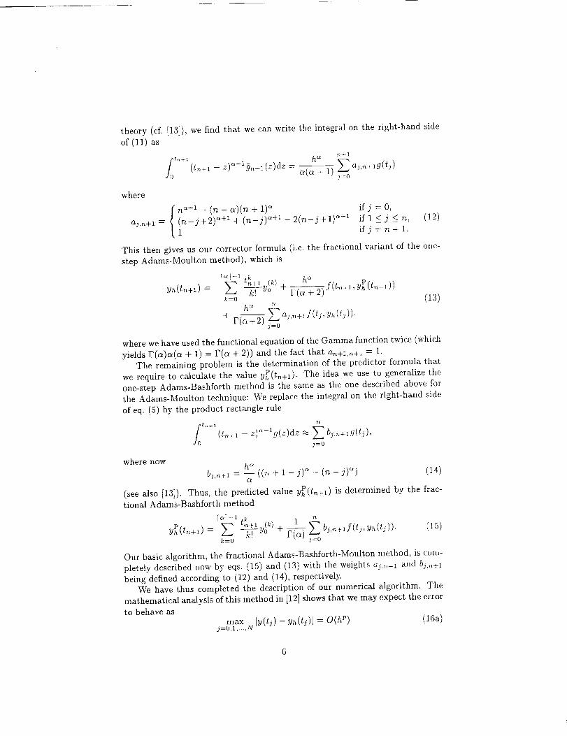
theory(cf. [131),wefind that wecanwritetheintegralon the right-hand side

of (11) as

f0 '_+_ (t_+l - z)a-10_+_ (z)dz -ha n+l

_(_ + 1)Z _j,...,g(tj)j=0

where we have used the functional equation of the Gamma function twice (which

yields r(a)a(ct + 1) = P(a + 2)) and the fact that an+m,n+l = 1.

The remaining problem is the determination of the predictor formula thatwe require to calculate the value yP(t,_+l). The idea we use to generalize the

one-step Adams-Bashforth method is the same as the one described above for

the Adams-Moulton technique: We replace the integral on the right-hand side

of eq. (5) by the product rectangle rule

fot°'_(t,_+l - z)_-lg(z)dz _ £ ba,,_+lg(t;),j=O

where now

(see also [13]).tional Adams-Bashforth method

;o,1-1 k £trt+l (k) 1 b£,_+lf(tj, yh(tj)). (15)

Our basic algorithm, the fractional Adams-Bashforth-Moulton method, is com-

pletely described now by eqs. (15) and (13) with the weights aa,,_+l and ba.,_+lbeing defined according to (12) and (14), respectively.

We have thus completed the description of our numerical algorithm. Themathematical analysis of this method in [12] shows that we may expect the errorto behave as

max ly(tj) - Yh(tj)l = O(h p) (16a)j----0,1,...,N

bj,_+l = -- ((n + 1 - j)_ - (n - j)a) (14)C[

Thus, the predicted value yPh(t_+l) is determined by the frac-

where

n a+m - (n - a)(n + 1) _ if j = 0,aj,n+l = (n-j+2)a+l+(n-j)a+l-2(n-j+l)a+l ifl<j_<n, (12)

1 ifj=n+l.

This then gives us our corrector formula (i.e. the fractional variant of the one-

step Adams-Moulton method), which is

[_]-1 k h_tn+l (k) f(tn+l,yP(tn+l))Y"(_+_)= _ -_U'y° + r(_+2)

k:0 (13)

+ r(_,+2-----7 _"_+'/(_' >(_J))'j=0

where

p = min(2, 1 + a) (]6b)

and the quantities h and N are related according to h = TIN, and T is theupper bound of the interval on which we are looking for the solution. The

reason for this rather special form of the exponent p is that one can prove that

p must be the minimum of the order of the corrector (which is 2 in our case)

and the order of the predictor method (which is 1 here) plus the order of the

differential operator (viz., a). This is a well known fact for PECE algorithms

for first-order equations (the case a = 1). In view of the fact that 1 < p < 2 wehave a satisfactory globally valid error bound. We note that, quite in contrast

to the behaviour of the algorithm described in [8], the convergence order p of theAdams-Bashforth-Moulton scheme increases as a, the order of the differential

equation, increases.

As far as the stability properties of our algorithm are concerend, we note that

it follows (unsing the general methods of Lubich [29]) that the stability prop-

erties of this fractional Adams-Bashforth-Moulton scheme are at least as good

as the corresponding properties of its counterpart for first-order equations, i.e.

the classical second-order Adams-Bashforth-Moulton method. The properties

of the latter are described in detail, e.g., in [25, Chap. IV].

For a more detailed investigation, including numerical examples, we refer to

[12]. The remainder of this paper will be devoted to more practical aspects.

Specifically in §3 we shall introduce some modifications that can enhance the

efficiency of our scheme, and in §4 we extend the capabilities of our integratorso that it can handle a more general class of equations. Finally we present some

numerical examples in §6, and for the convenience of the reader we also provide

an appendix where the algorithm is stated once again, but in a pseudo-code

type of notation.

3 Modifications of the Algorithm

We have completed the description of the basic algorithm and its most important

properties. Now we want to address the question of whether it is possible toimprove the performance of the algorithm in certain respects. There are indeed

a few ways to do this, and we shall mention some here. It is easily seen that most

of these modifications are independent of each other, so the user may implement

almost any combination of them as required.

3.1 Reduction of the arithmetic complexity

First of all, there is a fundamental problem associated with all fractional differ-

entiaI operators (not only the Caputo version that we look at here): In contrast

to differential operators of integer order, fractional derivatives are not local op-erators. This means that we cannot calculate D_.y(x), say, solely on the basis

of function values of y taken from a neighbourhood of the point x where we

work. R&ther, we have to take the entire history of y (i.e. all function values

y(t) for 0 < t < x) into account. This is clearly exhibited in the definition of theoperator, cf. eq. (2). As a matter of fact, this property is highly desirable from

the physical point of view because it allows us to model phenomena with mem-

ory effects. But when it comes to numerical work we find that this non-locality

leads to a significantly higher computational effort: The arithmetic complexity

of our algorithm with step size h is O(h-2), whereas a comparable algorithm for

an integer-order initial value problem (thus involving a local operator) would

only give rise to a O(h -1) complexity. A number of ways have been suggestedto overcome this difficulty. The first idea seems to have been the fixed memory

principle of Podlubny [31]. However a close mathematical analysis [13] reveals

that the reduced complexity is achieved at the price of a significant loss in the

order of accuracy of the method. A more promising approach seems to be the

nested memory concept of Ford and Simpson [21] that may well be applied to

our algorithm. This concept leads to an O(h -1 logh -1) complexity (so almostall of the additional work introduced by the non-locality is removed), and itcan be shown that this idea retains the order of accuracy of the underlying

algorithm. For more details we refer to [21].

3.2 Additional corrector iterations

Recall that in the case of a very stiff equation, we mentioned that the sta-

bility properties of the Adams-Bashforth-Moulton integrator may not be suffi-

cient. However, it is well known [24, 25] that the pure one-step Adams-Moulton

method (i.e. the trapezoidal method) possesses extremely good stability proper-

ties. These are spoiled in the Adams-Bashforth-Moulton approach only by the

fact that in eq. (13) we cannot replace the predictor approximation PYn-.-1 on tile

right-hand side by the correetor value yn+l because, in general, we cannot solve

that equation exactly any more. The idea is now to find a better approximationfor the exact solution of that equation than the rather simple one obtained by

applying just one functional corrector iteration with the predictor as a startingvalue.

There are two main ways to achieve this goal. The first one is to use the

value obtained by the first iteration (the first corrector step) as a new predictor

and apply another corrector step. Obviously, this procedure can be iterated

any given number of times, M say; the resulting method is called a P(EC)ME

algorithm. In this way, we find a method that is "closer" to the pure Adams-Moulton technique, and therefore, its stability properties are also closer to the

better properties of this method. Taking this idea to the extreme, we couldeven refrain from stopping after M iterations and continue to iterate until con-

vergence is achieved. This would (theoretically) lead to even better stability,but the computational cost could be prohibitive, and it may even happen that

(due to rounding errors) convergence could not be achieved numerically in finite

precision. Moreover the iteration may not converge unless the step size h ofthe method is sufficiently small. It is possible to make the P(EC)ME approach

more efficient by not using the same number M of corrector iterations in every

step. In regions of higher stiffness, more steps may be taken in order to retain

stabilityandto keeptheerrorundercontrol;whereas,inregionswherestiffnessisnotaproblem,highaccuracymaybeachievedalreadywithasmallchoiceofM, thus speeding up the algorithm.

In practice, one can implement this feature in such a way that the user can

supply an upper bound for the number M of corrector steps to be taken. Setting

this bound to 1 is then equivalent to switching off this modification completely.Moreover, the user can specify a tolerance c > 0 to the effect that the iteration

is stopped if two consecutive steps give results that differ by less than thistolerance even if the maximum number of iterations has not been reached.

In §4 we shall see that there also may exist other reasons for replacing the

plain PECE structure by a more complex P(EC)ME version with some suitableM.

As mentioned above, this is not the only possible approach to get a better

approximation to the solution of the corrector equation. The second idea that

we may use to enhance the stability of the method is to find another way ofsolving eq. (13) with PYn+l replaced by yn+l. The most obvious way to do this

would be to use a Newton iteration. As a starting value, we can still use the

Adams-Bashforth predictor. Since it is known that Newton iteration converges

faster (locally) than the simple functional iteration of the PECE process, wemay expect to come very close to the pure Adams-Moulton method in just a

few iterations. However, in order to implement Newton's method, we need to

work with the Jacobian of the right-hand side of the differential equation. This

can also be a source of numerical problems, and may even lead to very long run

times. We have, therefore, refrained from implementing and testing this so far,

but a future extension in this way is possible.

Note that, since we keep the Adams-Moulton formula as the basis of eq. (13),

the convergence order of these modified algorithms remains unchanged. More-

over, this modification of the algorithm does not alter the order of the arithmeticcomplexity in terms of the step size h. Only the stability is affected by these

modifications. Further, we stress that this modification (unlike the P(EC)ME

scheme) does not avoid the problems that we shall encounter in certain of thesituations mentioned in §4.

3.3 Richardson extrapolation

Whereas the suggestions above were constructed in order to improve the run

time or the stability of the algorithm without changing the convergence be-

haviour, we now turn our attention towards a possibile way of speeding up the

convergence. As noted in [12], numerical evidence suggets that the error of ourAdams scheme, taken to approximate the exact solution at a fixed point T > 0,

possesses an asymptotic expansion of the form

/:1 k2

y(T) - = c3h + j+° + O(h (17)j=l j=l

where kl, k2 and k3 are certain constants depending only on the solution y and

satisfying k3 > max(2kl, k2 + a). In practice it is unlikely that these constants

can be determined explicitly, but as a rule of thumb one may often work withsmall or moderate values like kl = 3 and k2 = 5. We shall see below that

knowledge of the value of ka is only necessary in order to derive an error bound

but not in order to actually implement the convergence speedup procedure•Notice that the asymptotic expansion begins with an h2 term and continues

with h1+_ for 1 < a < 3, whereas it begins with h _+a, followed by h2, for0<c_<l.

Our belief in the truth of this conjecture is not only supported by numer-

ical results but also by the theoretical analysis of de Hoog and Weiss [7, §5]

who show that asymptotic expansions of this form hold if we use the fractional

Adams-Moulton method (i.e. if we solve the corrector equation exactly) and that

a similar expansion can be derived for the fractional Adams-Bashforth method

(using the predictor as the final approximation rather than correcting once withthe Adams-Moulton formula). Assuming that the conjecture is correct, we may

use the relation (17) to eliminate the leading terms and thus obtain an approx-

imation that converges faster than the original one. According to the usual

constructions (cf., e.g., Walz I361), this results in a Richardson extrapolationscheme that has the following form• We begin by sorting the exponents of h

in eq. (17) in increasing order, thus obtaining a sequence jl, j2, j3,. •. where, in

the case 0 < a < 1, we have jl = 1 + a, j2 = 2, J3 = 2 + a, j4 = 3 + a, j5 = 4,

j6 =4+aetc-,whereasfor 1 <a < 2wehave31 = 2, j2 = l+a, j3 =2+a,

j4 = 4, j5 = 3+a, j6 = 4+a, etc. Obviously, we can proceed in a similar

way for the case a > 2, but since this latter case seems to be of minor practical

interest, we omit the details. Using this newly introduced terminology we can

rewrite the asymptotic expansion (17) for the error in the form

/(--1

y(T) - yh(T) = _ c'kh j_ + O(h jK) (18)k=l

with certain coefficients c_., some K E N and some positive real numbers j_ <j2 < "'" < jK. Note that, in a practical application, the jk are known by the

considerations above whereas the coefficients c; are in general unknown.The key observation is that we can use eq. (18) to improve the accuracy of our

approximation even though we do not know those coefficients c_. We proceed

by setting up a triangular array (a so-called Romberg tableau) of approximation

values for y(T) of the form

¢°2h i 2

Yht4y(o) _ (1)

h,18 b'h/8

_(2)his

• , o

10

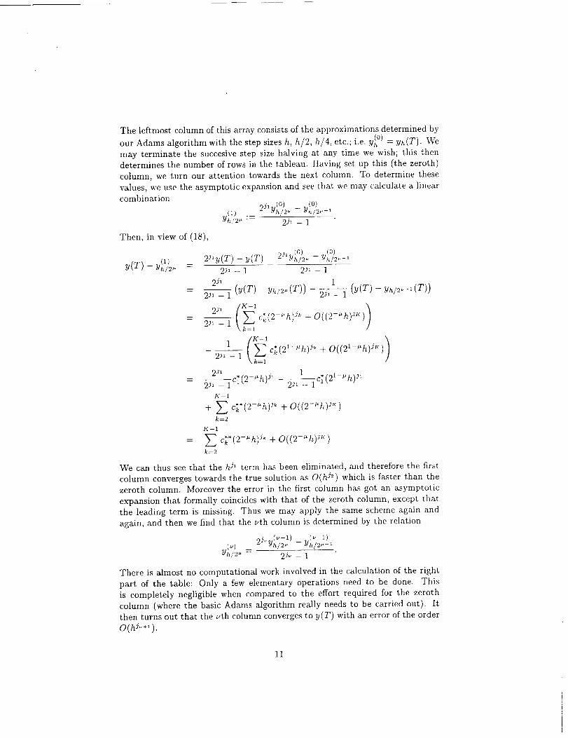
TheleffmostcolumnofthisarrayconsistsoftheapproximationsdeterminedbyourAdamsalgorithmwiththestepsizesh, h/2, h/4, etc.; i.e. y(h°) = yh(T). We

may terminate the succesive step size halving at any time we wish; this thendetermines the number of rows in the tableau. Having set up this (the zeroth)

column, we turn our attention towards the next column. To determine these

values, we use the asymptotic expansion and see that we may calculate a linear

combination2J'_(°) __(°)

. (1) ._ _h/2. ,Vh/2 .-1

9h/2, "-- 2 jl -- 1

Then, in view of (18),

y(Z) - yil/)2_,

2jl. (o) _ (o)2_'y(T) - y(T) _h/2,' -- Yt,/2,-'

2¢_ -- 1 2_' -- 1

2JI 1 (y(T) - Yh/2,-_ (T))= _ - t (y(T) - Y,_/2,(T)) 2Jl - 1

_2 j' -- 1 \ k=l

1(_'c*k(2'-_h)Jk+O((21-_'h)J'_))2 jl -- 1 \k=l

2jl 1 .= -- c1(21-"h)J'

2_1 - 1 2J1 - 1K-1

+ + O((2-"h)JK)k=2

K--1

= + o((2-"h) JK)k=2

We can thus see that the h jl term has been eliminated, and therefore the first

column converges towards the true solution as O(h j_) which is faster than the

zeroth column. Moreover the error in the first column has got an asymptotic

expansion that formally coincides with that of the zeroth column, except that

the leading term is missing. Thus we may apply the same scheme again and

again, and then we find that the uth column is determined by the relation

2j,,_,(u- 1) (w--l). (_) _'h/2*" -- Yh/2' "-1"{th/2" : 2 j_ -- 1

There is almost no computational work involved in the calculation of the right

part of the table: Only a few elementary operations need to be done. Thisis completely negligible when compared to the effort required for the zeroth

column (where the basic Adams algorithm really needs to be carried out). Itthen turns out that the _th column converges to y(T) with an error of the order

O(hJ_+').

11

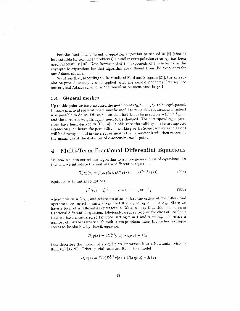
For the fractional differential equation algorithm presented in [8] (that is

less suitable for nonlinear problems) a similar extrapolation strategy has been

used successfully [16]. Note however that the exponents of the h-terms in the

asymptotic expansions for that algorithm are different from the exponents forour Adams scheme.

We stress that, according to the results of Ford and Simpson [21], the extrap-

olation procedure may also be applied (with the same exponents) if we replace

our original Adams scheme by the modification mentioned in §3.1.

3.4 General meshes

Up to this point we have assumed the mesh points to, tl, • • •, tN to be equispaced.

In some practical applications it may be useful to relax this requirement. Indeed

it is possible to do so. Of course we then find that the predictor weights bj,_+l

and the corrector weights aj,n+l need to be changed. The corresponding expres-

sions have been derived in [13, 14]. In this case the validity of the asymptotic

expansion (and hence the possibility of working with Richardson extrapolation)will be destroyed, and in the error estimates the parameter h will then representthe maximum of the distances of consecutive mesh points.

4 Multi-Term Fractional Differential Equations

We now want to extend our algorithm to a more general class of equations. To

this end we introduce the multi-term differential equation

,D.D, y(x) f(x,y(x),D_y(x),.., a.__

equipped with initial conditions

y(k)(0) = y_k), k = 0, 1,...,rn - 1,

(20a)

(2Oh)

where now m = [a_], and where we assume that the orders of the differential

operators are sorted in such a way that 0 < ch < c_2 < ..- < (_,- Since wehave a total of n differential operators in (20a), we say that this is an n-term

fractional differential equation. Obviously, we may recover the class of problemsthat we have considered so far upon setting n = 1 and a := a'_. There are a

number of instances where such multi-term problems arise; the earliest example

seems to be the Bagley-Torvik equation

bD3,/2y(x) + cy(x) + f(x)

rigid plate immersed into a Newtonian viscouscases are Babenko's model

D2,y(x) :

that describesthe motion of a

fluid (cf. [35, 9]). Other special

Dl, y(x) = F(x)D1,/2y(x) + G(x)y(x) + H(x)

12

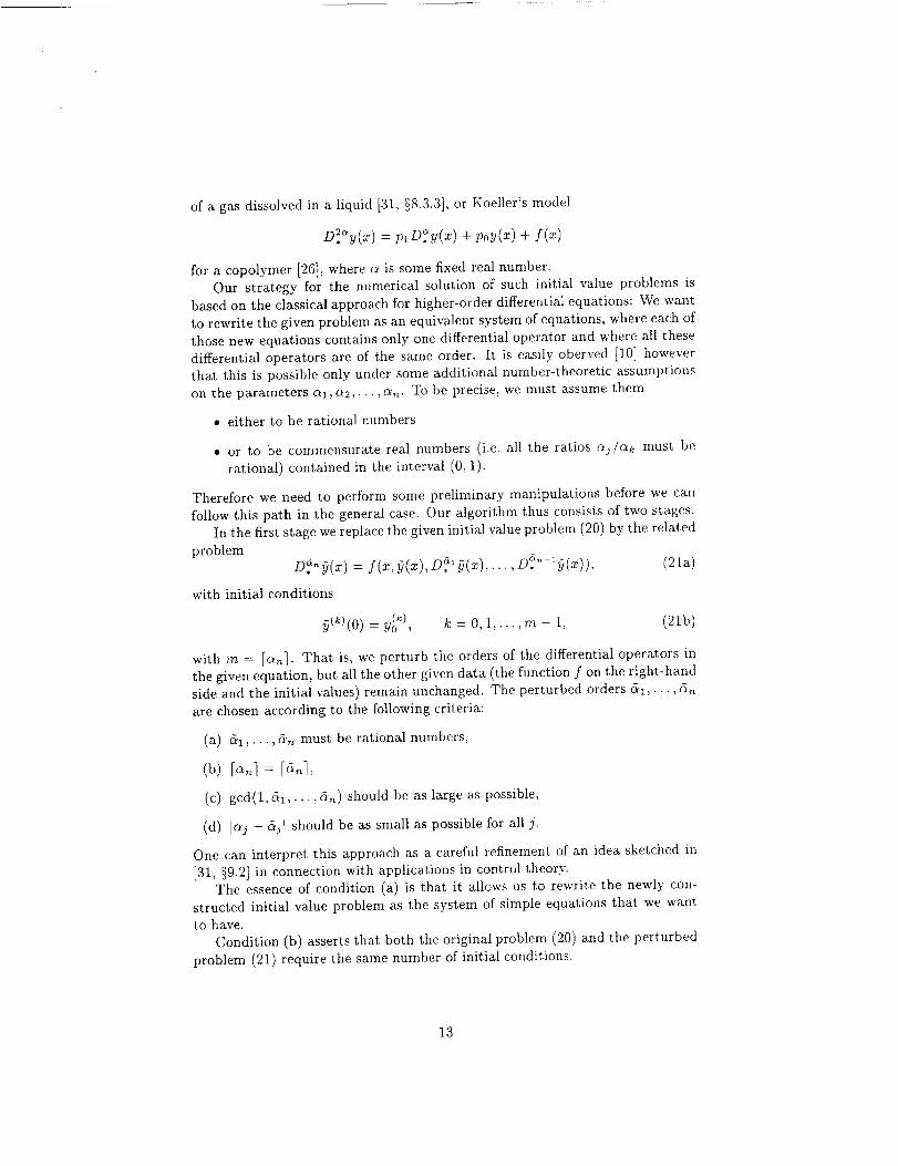
of agasdissolvedin a liquid[31,§8.3.3],orKoeller'smodel

= plD y(x) + poy(x) +

for a copolymer [26], where a is some fixed real number.

Our strategy for the numerical solution of such initial value problems is

based on the classical approach for higher-order differential equations: We want

to rewrite the given problem as an equivalent system of equations, where each of

those new equations contains only one differential operator and where all these

differential operators are of the same order. It is easily oberved /101 howeverthat this is possible only under some additional number-theoretic assumptions

on the parameters al, a2,..., a,. To be precise, we must assume them

• either to be rational numbers

• or to be commensurate real numbers (i.e. all the ratios aj/ak must be

rational) contained in the interval (0, 1).

Therefore we need to perform some preliminary manipulations before we can

follow this path in the general case. Our algorithm thus consists of two stages.

In the first stage we replace the given initial value problem (20) by the related

problem

: f(x,0(x),D. ,D. .... (21a)

with initial conditions

if(k)(0) = y_k), k = 0,1,...,m - 1, (21b)

with m = [c_]. That is, we perturb the orders of the differential operators inthe given equation, but all the other given data (the function f on the right-hand

side and the initial values) remain unchanged. The perturbed orders 51,.,., &,

are chosen according to the following criteria:

(a) &l, • -., 6'n must be rational numbers,

(b) ranl = ran],

(c) gcd(1, 51,..., &n) should be as large as possible,

(d) Jc_j - 5j] should be as small as possible for all j.

One can interpret this approach as a careful refinement of an idea sketched in

[31, _9.2] in connection with applications in control theory.The essence of condition (a) is that it allows us to rewrite the newly con-

structed initial value problem as the system of simple equations that we wantto have.

Condition (b) asserts that both the original problem (20) and the perturbed

problem (21) require the same number of initial conditions.

13

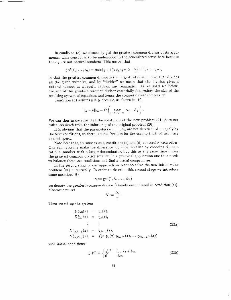
In condition(c),wedenotebygcdthegreatestcommondivisorof its argu-ments.Thisconceptis to beunderstoodin thegeneralizedsenseherebecausethe OLj are not natural numbers. This means that

gcd(zl,...,z,,) =max{q C Q:zj/q CN Vj = 1,2,...,n},

so that the greatest common divisor is the largest rational number that divides

all the given numbers, and by "divides" we mean that the division gives anatural number as a result, without any remainder. As we shall see below,

the size of this greatest common divisor essentially determines the size of the

resulting system of equations and hence the computational complexity.

Condition (d) assures 9 _ Y because, as shown in [10],

Hy-_)II_ =o ( max ]aj-Sjl _.\j=1,2 ..... ,_ /

We can thus make sure that the solution _ of the new problem (21) does not

differ too much fi'om the solution y of the original problem (20).

It is obvious that the parameters &l, • • •, an are not determined uniquely bythe four conditions, so there is some freedom for the user to trade off accuracy

against speed.Note here that, to some extent, conditions (c) and (d) contradict each other:

One can typically make the difference [&j - ajl smaller by choosing 5j as arational number with a larger denominator, but this at the same time makes

the greatest common divisor smaller. In a practical application one thus needsto balance these two conditions and find a useful compromise.

In the second stage of our approach we want to solve the new initial value

problem (21) numerically. In order to describe this second stage we introduce

some notation. By7 := gcd(1,&i,...,5,_)

we denote the greatest common divisor (already encountered in condition (c)).Moreover we set

OG z:z --.

?

Then we set up the system

D:yo(Z) = _(_),

n_,yl(x) = yz(x),

:

D_.y__,(x) = f(x,yo(x),ya,/._(x),...,y6._,/.r(x))

with initial conditions

yoJ'r) for j? E No,y_ (0) = 0 else,

(22a)

(22b)

14

andfind [10]that this isequivalentto theperturbedinitial valueprobleminthefollowingsense:Assumethatthesolutionofthesystemisthevector-valuedfunction(y0,...,YN-1),andthat 9 is thesolutionof (21).ThenYo = _).

We can immediately see that the dimension of the system is N, and by

definition of this quantity we see that this is large if 7 is small and vice versa.

This justifies condition (c) above.

The initial conditions (22b) correspond to the given initial conditions in the

sense that those components of (Yo,...,Y__I) that correspond to an integer-order derivative of 9 are assigned that initial value, whereas all other initial

values are set to zero. A mathematical justification of this choice is given in [9];

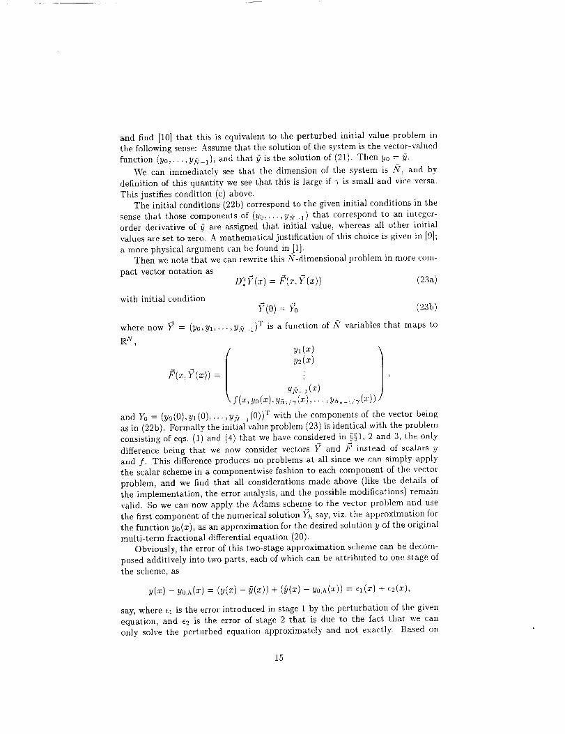
a more physical argument can be found in [I].Then we note that we can rewrite this N-dimensional problem in more com-

pact vector notation as

D_,Y(x) = F(z, Y(x)) (23a)

with initial condition

I7(0) = 17o (23b)

where now 17 = (Yo,Y_,... ,YR_I) T is a function of fi,r variables that maps to

II@? ,

w(x)f(x, f(x)) = • ,

f (x,yo(x),w,/,(x), . . . , )

and Y0 = (yo(0), Yl (0),... Y_-I (0)) T with the components of the vector being

as in (22b). Formally the initial value problem (23) is identical with the problem

consisting of eqs. (1) and (4) that we have considered in §§1, 2 and 3, the only

difference being that we now consider vectors }7 and /Y instead of scalars y

and f. This difference produces no problems at all since we can simply applythe scalar scheme in a componentwise fashion to each component of the vector

problem, and we find that all considerations made above (like the details ofthe implementation, the error analysis, and the possible modifications) remain

valid. So we can now apply the Adams scheme to the vector problem and use

the first component of the numerical solution _ say, viz. the approximation for

the function yo(x), as an approximation for the desired solution y of the original

multi-term fractional differential equation (20).

Obviously, the error of this two-stage approximation scheme can be decom-posed additively into two parts, each of which can be attributed to one stage of

the scheme, as

- yo,h( ) = - + - y0,h(x))= +

say, where q is the error introduced in stage 1 by the perturbation of the given

equation, and ez is the error of stage 2 that is due to the fact that we can

only solve the perturbed equation approximately and not exactly. Based on

15

this decompositionit mayseemtemptingto reducetheoverallerrorsimplyby reducingthecontributionfromq andleavingstage2 unchanged.In viewof whatwesaidabove,this caneasilybeachievedby choosingthe6d values

closer to the original aj. However, we repeat that this is likely to increase thedimension of the system, and the very structure of the system (to be precise: the

large number of zeros in the initial condition (22b)) has the unwanted effect of

making this more precise system much more difficult to handle for a numerical

integration scheme. Thus it will often be observed that the cavalier approach of

improving in stage 1 and not changing stage 2 will lead to a small improvement

in q at the price of a major deterioration of _2 and hence a worse overall result.

5 Further work

One area that needs further investigation is this last dilemma. We have identified

two possible ways forward, but the question remains open as to which of these

(or some other approach) would be more appropriate.

The first option we have identified is to decrease the step size h used in stage2 as the dimension fig of the system increases (a useful rule of thumb would be

to use h = c/fig with some constant c).

Our second approach would be to remove those zeros (that do not contribute

to the overall solution, so that the numerical solution gets stuck at the initial

value for the first approximately 1/(27) steps) by replacing the plain PECE

structure by a P(EC)ME version with a sufficiently large M (e.g. M = 1/?').One could also combine these two ideas or use different values of M in

different regions. For the present we can say that these two approaches both have

the disadvantage of a significant increase in the computational effort, so one may

often be better off with a quite crude approximation in the first stage followed

by a simple version of the approximation algorithm in the second stage. This

is particularly true if the given orders oh,..., c_ of the differential operators in(20a) are something like material constants that are known only up to a limited

accuracy.

6 Numerical Examples

In this section we present some numerical examples to illustrate the error bounds

derived above. We only considered examples where 0 < (_ < 2 since the case a

2 does not seem to be of major practical interest. In all cases, the computationswere performed in the usual double precision arithmetic on a Pentium-basedPC.

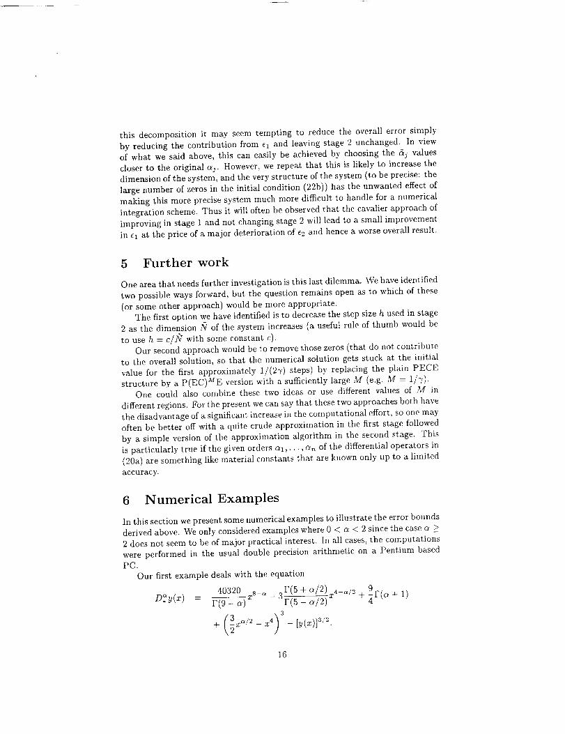
Our first example deals with the equation

40320- 3r(5 + _/2)_ 4-_/2 + _r(_ + 1)D*_Y(z) = r(9- _)zs-_ r(5- 4/2)

+ (_°/_ - _4) 3 - [y(_)]3/2.

16

Theinitial conditionswerechosento behomogeneous(y(0)= 0,y'(0) = 0; the

latter only in the case a > 1). The exact solution of this initial value problemis

9y(x) = x s - 3x 4+a/2 -k _x .

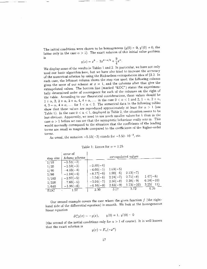
We display some of the results in Tables 1 and 2. In particular, we have not only

used our basic algorithm here, but we have also tried to increase the accuracy

of the numerical solution by using the Richardson extrapolation idea of §3.3. In

each case, the leftmost column shows the step size used; the following columngives the error of our scheme at x = 1, and the columns after that give the

extrapolated values. The bottom line (marked "EOC") states the experimen-

tally determined order of convergence for each of the columns on the right of

the table. According to our theoretical considerations, these values should be

1 + _, 2, 2 + _, 3 + a, 4, 4 + a, ... in the case 0 < a. < 1 and 2, 1 + _, 2 + a,

4, 3 + a, 4 + a, ... for 1 < a < 2. The numerical data in the following tables

show that these values are reproduced approximately at least for a > 1 (see

Table 1). In the case 0 < a < 1, displayed in Table 2, the situation seems to beless obvious. Apparently, we need to use much smaller values for h than in the

case a > 1 before we can see that the asymptotic behaviour really sets in. This

would normally correspond to the situation that. the coefficients of the leadingterms are small in magnitude compared to the coefficients of the higher-orderterms.

As usual, the notation -5.53(-3) stands for -5.53- 10 -3 , etc.

Table 1: Errors for c_ = 1.25.

step size

1/lO1/2o1/4o1/8o1/160

1/3201/640EOC

error of

Adams scheme

-5.53(-3)-1.59(-3)-4.33(-4)-1.14(-4)-2.97(-5)-7.66(-6)-1.96(-6)

1.97

extrapolated values

-2.80(-4)-4.6O(-5) 1.63(-5)-8.17(-6) 1.90(-6) 2.13(-7)-1.54(-6) 2.24(-7) 2.71(-8) 1.47(-8)-3.04(-7) 2.56(-8) 2.28(-9) 6.24(-10)-6.16(-8) 2.85(-9) 1.73(-10) 3.25(-11)

2,30 3.17 3.72 4.26

Our second example covers the case where the given function f (the right-

hand side of the differential equation) is smooth. We look at the homogeneous

linear equation

D.%(x) = -y(x), y(0) = 1, y'(0) = 0

(the second of the initial conditions only for a > 1 of course). It is well knownthat the exact solution is

y(z) = E_(-z _)

17

stepsize1/lO1t2o1/40

1/8o1/160

1/32o1/640EOC

Table 2: Errors for a = 0.25.

error ofAdams scheme

2.5o(-1)1.81(-2)3.61(-3)1.45(-3)6.58(-4)2.97(-4)1.31(-4)

1.18

extrapolated values

-1.50(-1)-6.91(-3) 4.09(-2)-1.10(-4) 2.16(-3) -8.15(-3)

8.19(-5) 1.46(-4) -3.89(-4) 1.28(-4)3.49(-5) 1.92(-5) -1.45(-5) ].05(-5)1.12(-5) 3.37(-6) -s.50(-r) 6.01(-8)

1.63 2.51 4.09 7,44

where

_(z) = p(_k + 1)k=0

is the Mittag-Leffler function of order a.In Table 3 we state some numerical results for this problem in the case a < 1.

The data given in the tables is the error of the Adams scheme at the point x = 1.We can see from the last line that the order of convergence is always close to

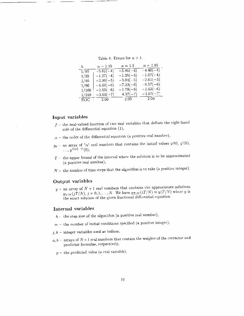
1 + a. In contrast, Table 4 displays the case a > 1; here the results confirm the

O(h 2) behaviour. This reflects the statement of eq. (16).

1/10

1/201/40

1/8o1/16o1/32oEOC

Table 3: Errors for a < 1.

a=0.1 c_ = 0.3 c_ = 0.5 a=0.7 a=0,9

-5.42(-3) -1.86(-3) -1.30(-3) -9.91(-4) -7.51(-4)

-1,22(-3) -5.85(-4) -3,93(-4) -2,81(-4) -1,91(-4)

-4.40(-4) -1.97(-4) -1,26(-4) -8.28(-5) -4.99(-5)

-1.68(-4) -6.90(-5) -4,18(-5) -2.50(-5) -1.32(-5)-6.65(-5) -2.49(-5) -1.42(-5) -763(-6) -3.54(-6)

-2.68(-5) -9.18(-6) -4.86(-6) -2.35(-6) -9.48(-7)1.31 1.44 1.54 1.70 1.90

Appendix: Pseudo code of the algorithm

Following the derivation and description of the Adams-Bashforth-Moulton al-

gorithm in mathematical terms given in §2 we now state this algorithm in a

pseudo code type notation. In this way the reader interested in implementing

the method can easily do so in the language of his or her preference.

18

h

111o

1/2o1t4ol/SO1/160

11320EOC

Table 4: Errors for a > 1.

c_ = 1.25 a = 1.5 a = 1,85

-5.61(-4) -5.46(-4) -4.40(-4)

-1.27(-4) -1.28(-4) -1.07(-4)-2.90(-5) -3.04(-5) -2.65(-5)

-6.68(-6) -7.33(-6) -6.57(-6)

-1.55(-6) -1.78(-6) -1.63(-6)

-3.63(-7) -4.37(-7) -4.07(-7)2.09 2.03 2.00

Input variables

f - the real-valued function of two real variables that defines the right-hand

side of the differential equation (1),

a - the order of the differential equation (a positive real number),

yo - an array of [a] real numbers that contains the initial values y(0), y'(0),

..., y(l_7-1t(0),

T - the upper bound of the interval where the solution is to be approximated

(a positive real number),

N - the number of time steps that the algorithm is to take (a positive integer).

Output variables

y - an array of N + 1 real numbers that contains the approximate solutions

yT/N(jTIN), j = O, 1,..., N. W'e have yTtJv(jT/N) _. y(T/N) where y isthe exact solution of the given fractional differential equation.

Internal variables

h - the step size of the algorithm (a positive real number),

m - the number of initial conditions specified (a positive integer),

j, k - integer variables used as indices,

a, b - arrays of N + 1 real numbers that contain the weights of the corrector and

predictor formulae, respectively,

p - the predicted value (a real variable).

19

Comment

In orderto savememory,thearraysa andb are one-dimensional and not two-dimensional as indicated by the notation in §2. This is possible because the

values a3,k and bd,k defined in eqs. (12) and (14), respectively, essentially havea convolution structure, i.e. they only depend on the difference k - j of the twoindices.

Body of the procedure

h := T/N

FOR k := 1 TO N DO BEGIN

b[k] := k ° - (k - 1) _

a[k] := (k + 1) _+1 - 2k _+1 + (k - 1) _+_

END

y[o] := yo[o]

FOR j := 1 TO N DO BEGIN

._-1 (jh)k ._ he j-1p := _ --_._ yot_j + F(a + 1) __b[j - k]f(hh, y[k])

k0k=0

_-_ (jh)k ,,_[j] := _ --g-, yo[_j

k----0

END

+ F(c_+2_ f(jh,p)+ ((j- 1) a+l-(j- 1-c_)9 ) f(0,y[0])

J-_ )+ E a[j - k]f(kh, y[k])k=l

References

[1] R. L. BAGLEY AND R. A. CALICO, Fractional order state equations for

the control of viscoeIastically damped structures, J. of Guidance, Control

and Dynamics, 14 (1991), pp. 304-311.

[2] D. A. BENSON, The Fractional Advection-Dispersion Equation: Develop-ment and Application, Ph. D. thesis, University of Nevada Reno, 1998.

2O

[3] L. BLANK, Numerical treatment of differential equations of fractional or-der, Numerical Analysis Report 287, Manchester Centre for Computational

Mathematics, 1996.

[4] P. L. BUTZER AND U. WESTPHAL, An introduction to fractional calculus,

in Applications of Fractional Calculus in Physics, R. Hilfer, ed., World

Scientific Publ. Comp., Singapore, 2000, pp. 1-85.

[5] M. CAPUTO, Linear models of dissipation whose Q is almost frequency

independent, II, Oeophys. J. Royal Astronom. Soc., 13 (1967), pp. 529-539.

[6] J.-T. CHERN, Finite Element Modeling of Viscoelastic Materials on the

Theory of Fractional Calculus, Ph. D. thesis, Pennsylvania State University,1993.

[7] F. DE HOOG AND R. V_TEISS, Asymptotic expansions for product integra-

tion, Math. Comp., 27 (1973), pp. 295-306.

[8] K. DIETHELM, An algorithm for the numerical solution of differential equa-

tions of fractional order, Elec. Transact. Numer. Anal., 5 (1997), pp. 1-6.

[9] K. DIETHELM AND N. J. FORD, Numerical solution of the Bagley-Torvik

equation, Berichte der Mathematischen Institute 00/]4, Technische Univer-

sit£t Braunschweig, 2000 (http://www.tu-bs.de/_diethelm/publications/bteq.ps). Submitted for publication.

[10] K. DIETHELM AND N. J. FORD, Numerical solution of linear and

non-linear fractional differential equations involving fractional deriva-tives of several orders, Numerical Analysis Report 379, Manchester Cen-

tre for Computational Mathematics, 2001 (http://www.maths.man.ac.uk/

_nareports/narep379.ps.gz). Submitted for publication.

[11] K. DIETHELM AND N. J. FORD, Analysis of fractional differential equa-

tions, J. Math. Anal. Appl., 265 (2002), in press.

[12] K. DIETHELM, N. J. FORD, AND A. D. FREED, Full error analysis for a

fractional Adams method, (in preparation).

[13] K. DIETHELM AND A. D. FREED, The FracPECE subroutine for the nu-

merical solution of differential equations of fractional order, in Forschungund wissenschaftliches Rechnen 1998, S. Heinzel and T. Plesser, eds., no. 52

in GWDG-Berichte, GSttingen, 1999, Gesellschaft flit wissenschaftliche

Datenverarbeitung, pp. 57-71.

[14] K. DIETHELM AND A. D. FREED, On the solution of nonlinear fractional

differential equations used in the modeling of viscoplasticity, in Scientific

Computing in Chemical Engineering II -- Computational Fluid Dynam-

ics, Reaction Engineering, and Molecular Properties, F. Keil, W. Mackens,H. Vofl and J. Werther, eds., Heidelberg, 1999, Springer, pp. 217-224.

21

[15] K. DIETHELM AND Y. LUCHI<O, Numerical solution of linear multi-term

initial value problems of fractional order, J. Comput. Anal. Appl., to ap-

pear.

[16] K. DIETHELM AND G. WALZ, Numerical solution of fractional order differ-

ential equations by extrapolation, Numer. Algorithms, 16 (1997), pp. 231-

253.

[17} M. ENELUND, A. FENANDER, AND P. OLSSON, Fractional integral for-

mulation of constitutive equations of viscoelasticity, AIAA J., 35 (1997),

pp. 1356-1362.

[18] M. ENELUND AND B. L. JOSEFSON, Time-domain finite element analysis

of viscoelastic structures with fractional derivative constitutive relations,

AIAA J., 35 (1997), pp. 1630-1637.

[19] M. ENELUND AND G. A. LESIEUTRE, Time domain modeling of damping

using anelastic displacement fields and fractional calculus, Int. J. Solids

Structures, 36 (1998), pp. 4447-4472.

[20] M. ENELUND AND P. OLSSON, Damping descmbed by fading memory --

Analysis and application to fractional derivative models, Int. J. Solids Struc-

tures, 36 (1998), pp. 939-970.

[211 N. J. FORD AND A. C. SIMPSON, The numerical solution of fractional dif-

ferential equations: Speed versus accuracy, Numer. Algorithms, 26 (2001),

pp. 333-346.

[22] R. GORENFLO, Fractional calculus: Some numerical methods, in Frac-

tals and Fractional Calculus in Continuum Mechanics, A. Carpinteri and

F. Mainardi, eds., Wien, 1997, Springer, pp. 277-290.

[231 R. GORENFLO AND F. _/IAINARDI, Fractional calculus: Integral and differ-

ential equations of fractional order, in Fractals and Fractional Calculus in

Continuum Mechanics, A. Carpinteri and F. Mainardi, eds., Wien, 1997,

Springer, pp. 223-276.

[24] E. HAIRER, S. P. Nq_RSETT, AND G. VVANNER, Solving Ordinary Dzf-

ferential Equations I: Nonstiff Problems, Springer, Berlin, 2nd revised ed.,

1993.

[25] E. HAIRER AND G. WANNER, Solving Ordinary Differential Equations II:

Stiff and Differential-Algebraic Problems, Springer, Berlin, 1991.

[26] R. C. KOELLER, Polynomial operators, Stieltjes convolution, and fractional

calculus in hereditary mechanics, Acta Mech., 58 (1986), pp. 251-264.

[27] C. F. LORENZO AND T. T. HARTLEY, Initialized fractional calculus, Int.

J. Appl. Math., 3 (2000), pp. 249-265.

22

[28] C. LUBICH, Runge-Kutta theory for Volterra and Abel integral equations of

the second kind, Math. Comp., 41 (1983), pp. 87-102.

[29] C. LUBICH, Fractional linear multistep methods for Abel-Volterra integralequations of the second kind, Math. Comp., 45 (1985), pp. 463--469.

[30] C. LUBICH, Discretizedfractional calculus, SIAM J. Math. Anal., 17 (1986),pp. 704-719.

[31] I. PODLUBNY, Fractional Differential Equations, Academic Press, San

Diego, 1999.

[32] P. RUGE AND N. WAGNER, Time-domain solutions for vibration sys-terns with fading memory, In Proceedings of the European Conference

on Computational Mechanics 1999. CD-ROM, Lehrstuhl fiir Statik, Tech-

nische Universit/it M/inchen (http://www.isd.uni-stuttgart.de/_nwagner/

eccm99.ps).

[33] S. G. SAMKO, A. A. KILBAS, AND O. I. MARICHEV, Fractional Integrals

and Derivatives: Theory and Applications, Gordon and Breach, Yverdon,1993.

[34] A. SHOKOOH AND L. E. SUAREZ, A comparison of numerical methodsapplied to a fractional derivative model of damping materials, J. Vibration

Control, 5 (1999), pp. 331-354.

[35] P. J. TORVIK AND R. L. BAGLEY, On the appearance of the fractional

derivative in the behavior of real materials, J. App]. Mech., 51 (t984),

pp. 294-298.

[36] G. WALZ, Asymptotics and Extrapolation, Akademie-Verlag, Berlin, 1996.

[37] L. YUAN AND O. P. AGRAWAL, A numerical scheme for dynamic systemscontaining fractional derivatives, Proceedings of the ]998 ASME Design

Engineering Technical Conferences (September 13-16, 1998, Atlanta, Geor-

gia). CD-ROM, ASME International, New York, 1998, ISBN 0791819531

(http: / /heera.engr.siu.edu/mech/faculty /agrawal/mech5857.pdf).

23