Numerical Simulation of Wind Wave Field · Numerical Simulation of Wind Wave Field Lihwa Lin 1, Ray-Qing Lin 2, and Jerome P.Y. Maa3 1 U.S. Army Engineer Research and Development

Numerical Simulation of Wind Wave Field

Lihwa Lin 1, Ray-Qing Lin 2, and Jerome P.Y. Maa3

1 U.S. Army Engineer Research and Development Center 3909 Halls Ferry Road, Vicksburg, MS. 39180

2 David Taylor Model Basin, Division of Seakeeping,

9500 MacArthur Blvd, West Bethesda, NSWCCD, MD 20817-5700

3 Virginia Institute of Marine Science, School of Marine Science Route 1208, Greate Road, Gloucester Point, VA 23062

1. INTRODUCTION Water waves observed in the field are the result of combined mechanics of wave generation, dissipation, propagation, and nonlinear wave-wave interactions. In physical terms, the wave generation and dissipation are essentially source and sink functions, respectively, responsible for the wave energy growth and decay. The propagation and nonlinear wave-wave interactions, on the other hand, are accounted for straight wave transformation and evolution that the energy is conserved in these processes. In applications, it is necessary to formulate individual terms of generation, dissipation, and nonlinear wave-wave interactions for accurate calculations of the combined physics in the wave field. Because natural gravity waves normally appear in irregular forms and propagate in scattered directions, directional spectral transformation models shall be used for the calculation of a wave field. The directional spectrum propagation scheme including linear wave shoaling and refraction has been well developed in the past. Some recent efforts have included wave diffraction and reflection in the spectral energy propagation scheme (Lin and Demirbilek, 2005). Theoretical and numerical formations of nonlinear wave-wave interactions are also well studied and documented in the last two decades (Lin and Perrie, 1997, 1999). Lin and Lin (2002, 2006) have used the field data to illustrate the nonlinearity of spectral wave energy transfer. There are a number of formulas applied for wave generation and dissipation in spectral wave models. However, because of the general difficulty separating data for wave growth and decay, formulating and calibrating these source and sink functions are the least satisfaction in the model. In previous studies, authors have proposed both wind input and wave breaking functions based on physical interpretations and calibrated with field data (Lin and Lin, 2004a, 2004b). In the present study, these wind input and wave breaking functions are applied in a directional spectral model and verified with two available data sets collected independently in the field. The first data set is collected in the lower Chesapeake Bay and used in the investigation of new wave generation under a strong wind condition. The second data set is collected at the mouth of Columbia River, OR/WA, for the investigation of directional spectral evolution in the near shore under either weak or moderate wind speeds. Calculated directional spectra at these two sites generally compare well with the data. Because the nonlinear wave energy transfer is not simulated in the model, the calculated directional spectrum is skewed to higher frequencies. 2. NUMERICAL MODEL Lin and Lin (2004a, 2004b) have investigated wind input and wave dissipation functions using the field data. This paper presents the continued study and applies these wind input and wave breaking functions to simulate the wind wave filed. A Wave-Action Balance Equation with Diffraction (WABED) model is used to calculate the wave field for a steady sea state (Mase 2001; Mase et al. 2005; Lin et al. 2006):

2 2[( ) ] [( ) ] [ ] 1{( cos ) cos }2 2

gx gy gg y y g yy in dp

c u A c v A c Acc A cc A S S

x yθ κ θ θθ σ

∂ + ∂ + ∂+ + = − + +

∂ ∂ ∂

(1) where /A E σ= is the wave action density, defined as the ratio of spectral energy density ( , )E E σ θ=

to intrinsic frequency σ ; gxc , gyc , and θgc are group velocities relative to x, y (eastern and northern

axes of the water surface), and θ (angle between north and wavelet direction), respectively; u and v are the current velocity components in the x and y directions, respectively. inS is a source term for the energy

growth and dsS is a sink term for the energy dissipation. The nonlinear wave-wave interaction is not included in Eq. (1). The wave diffraction is presented by the first term in the right hand side of Eq. (1), where the parameterκ controls the intensity of wave diffraction. In the present study, the WABED solves Eq. (1) by a forward-marching, finite-difference method on a half plane so primary waves can propagate only from the seaward boundary toward shore. The current effect on waves is included in the model as a Doppler shift in the solution of intrinsic frequency calculated through the wave dispersion equation. This treatment of the wave-current interaction is considered in other similar models (Smith et al. 1999; Lin and Demirbilek 2005). 2.1 Wind Input Function The rate of wind-input is formulated as functions of the ratio of wave celerity c to wind speed w, the ratio of wave group velocity to wind speed, the difference of wind speed and wave celerity, and the angle difference between wind direction windθ and wave directionθ (Lin and Lin, 2004b):

*1 21 2 1 2 3( ) ( ) ( ) ( ) ( ) ( ) ( )in PM

a ac c cS F w c F E F w c F F Eg w g w wσ σσ θ= − Φ + −

r r r r (2)

where 1

cos( ) ,( )

0,windw c

F w cθ θ− −⎧

− = ⎨⎩

r r ifif

c wc w<≥

0.8

2( ) ,( )1,

gg

ccF ww

⎧⎪= ⎨⎪⎩

ifif

g

g

c w

c w

<

≥

1

103

log [( ) ],( )

0,

ccF ww

−⎧⎪= ⎨⎪⎩

ifif

c wc w<≥

and 42

* 05 4( ) exp( 0.74 )PM

gE σσσ σ

= − .

Here, )(* σPME is the functional form of Pierson-Moskowitz (PM) spectrum, 0 /g wσ = is the Phillips’s constant, and

)(cos38)( 4

windθθπ

θ −=Φ for 2/|| πθθ <− wind .

is a normalized directional spreading. Function 1F is due to the wind stress effect, 2F is due to Phillips’

mechanisms (Phillips, 1957) and 3F is due to the wave age effect. For long waves (developed or “old”

waves), the phase velocity is generally large and 3F < 1. If wc ≥ , then 3F =0. For short waves

(“young” waves), the phase velocity is generally small and 3F > 1. 2.2 Wave Dissipation Function The wave breaking function including whitecapping and turbulent viscous dissipation effects is (Lin and Lin, 2004a)

4 51.5( ) ( , ) ( , , ) ( )dp ds g current gS C ak c F w u c F kh E

gσ σ θ= −

r r r (3)

with 4 ( , , )current gcurrent g

wF w u cw u c

υ +=

+ +r r r

r r r and 51( )

tanhF kh

kh=

where dsC is a proportional constant and υ is for the turbulent viscous dissipation. The wavelet amplitude

( , )d dEa σ θ σ θ= is calculated at each grid cell. To avoid the numerical instability and consider the

physical constraint of energy loss for the dissipation, the function F4 is set to equal to 1 if the computed value is greater than 1. 2.3 Bottom Frictional Loss The additional dissipation rate attributed to bottom friction is also calculated (Collins, 1972):

2, sinhb

fdp fricuS C E

g khσ < >

= − with < bu >12 total

g Eh

= (4)

where < bu > presents the ensemble mean of horizontal wave orbital velocity at the sea bed and totalE is the total energy density at a grid cell.

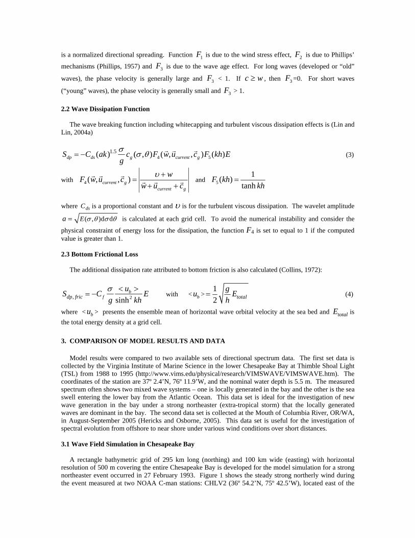
3. COMPARISON OF MODEL RESULTS AND DATA Model results were compared to two available sets of directional spectrum data. The first set data is collected by the Virginia Institute of Marine Science in the lower Chesapeake Bay at Thimble Shoal Light (TSL) from 1988 to 1995 (http://www.vims.edu/physical/research/VIMSWAVE/VIMSWAVE.htm). The coordinates of the station are 37º 2.4’N, 76º 11.9’W, and the nominal water depth is 5.5 m. The measured spectrum often shows two mixed wave systems – one is locally generated in the bay and the other is the sea swell entering the lower bay from the Atlantic Ocean. This data set is ideal for the investigation of new wave generation in the bay under a strong northeaster (extra-tropical storm) that the locally generated waves are dominant in the bay. The second data set is collected at the Mouth of Columbia River, OR/WA, in August-September 2005 (Hericks and Osborne, 2005). This data set is useful for the investigation of spectral evolution from offshore to near shore under various wind conditions over short distances. 3.1 Wave Field Simulation in Chesapeake Bay A rectangle bathymetric grid of 295 km long (northing) and 100 km wide (easting) with horizontal resolution of 500 m covering the entire Chesapeake Bay is developed for the model simulation for a strong northeaster event occurred in 27 February 1993. Figure 1 shows the steady strong northerly wind during the event measured at two NOAA C-man stations: CHLV2 (36º 54.2’N, 75º 42.5’W), located east of the

lower bay entrance, and TPLM2 (38º 53.5’N, 76º 26.1’W), located in the middle of the narrow upper bay (http://www.ndbc.noaa.gov/maps/Chesapeake_Bay.shtml). During this strong wind event, large waves were observed at Stations CHLV2 and TSL (Figure 1). Figure 2 shows (a) the model bathymetric domain, and (b) calculated wave field under a steady northerly wind (15 m/sec from north) at 12:00 GMT, 27 February 1993. Figure 3 compares measured and calculated directional spectra at Station TSL. The magnitude and direction of calculated spectrum agree well with the measured. The effect of nonlinear wave-wave interactions from higher to lower frequency is clearly seen in the measured spectrum. Because this nonlinearity of energy transfer is not simulated in the model, the calculated spectrum is significantly skewed to higher frequency. Therefore, the nonlinear wave energy transfer is evidently strong and important in the wind wave generation and should be incorporated in the model calculations.

Figure 1. Wave and wind data collected at Stations CHLV2, TPLM2, and TSL, 21-29 February 1993 – an extra-tropical event for the illustration of wind wave generation is shown in circles

Extra-tropical storm

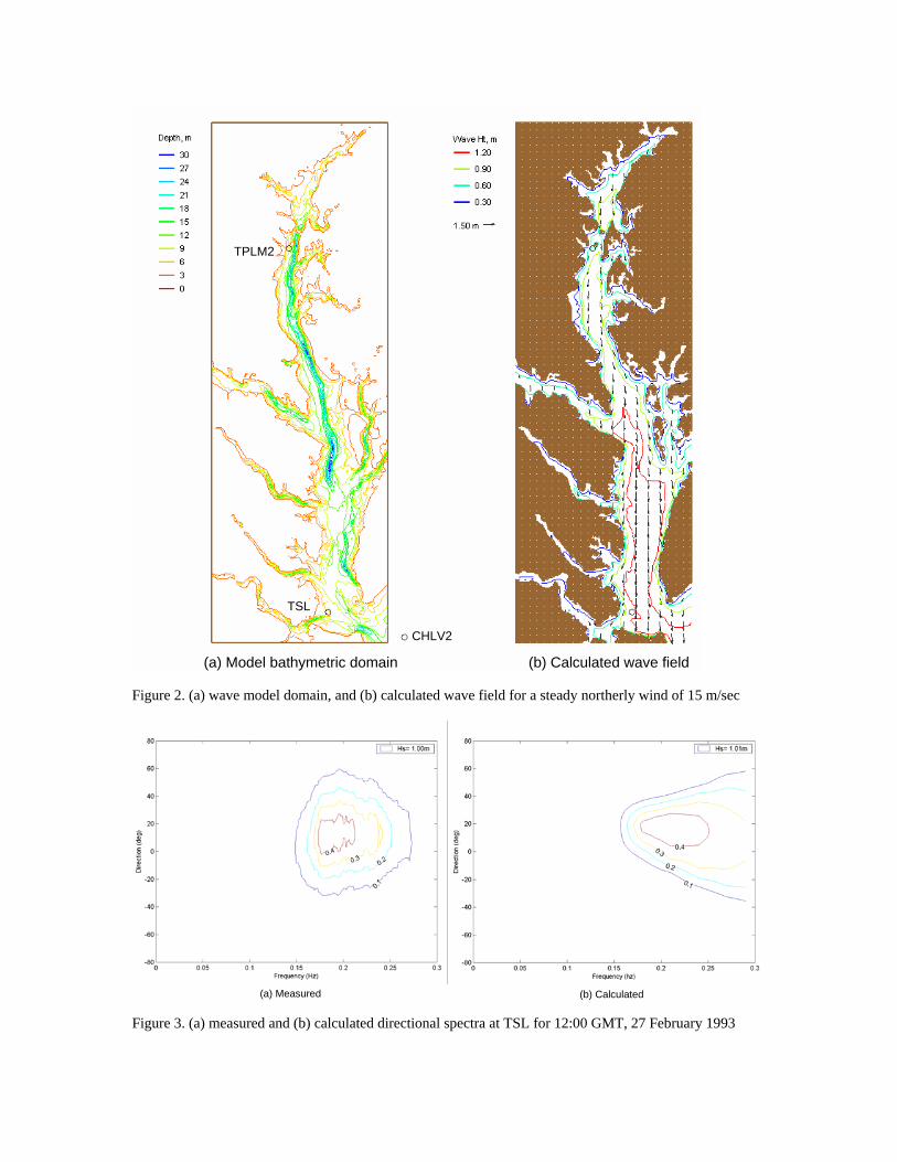
Figure 2. (a) wave model domain, and (b) calculated wave field for a steady northerly wind of 15 m/sec

Figure 3. (a) measured and (b) calculated directional spectra at TSL for 12:00 GMT, 27 February 1993

CHLV2

TPLM2

TSL

(a) Model bathymetric domain (b) Calculated wave field

(a) Measured (b) Calculated

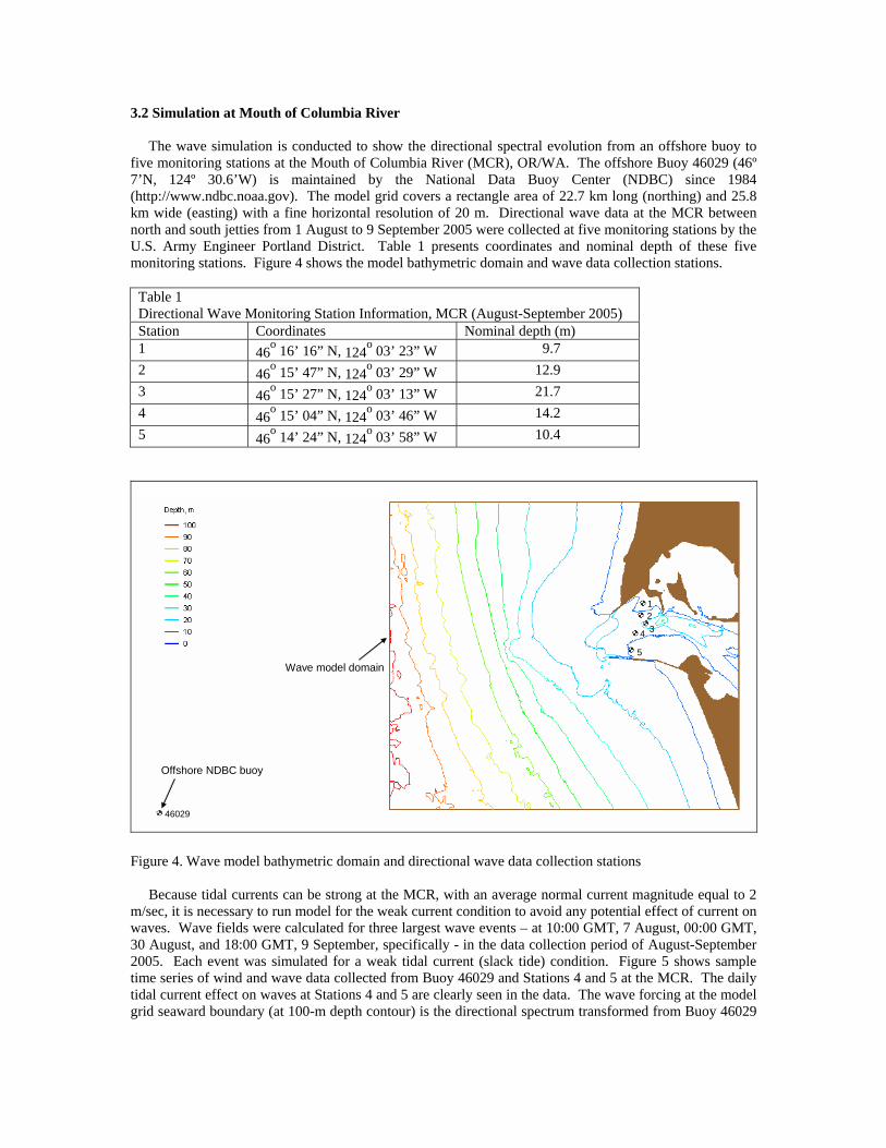
3.2 Simulation at Mouth of Columbia River The wave simulation is conducted to show the directional spectral evolution from an offshore buoy to five monitoring stations at the Mouth of Columbia River (MCR), OR/WA. The offshore Buoy 46029 (46º 7’N, 124º 30.6’W) is maintained by the National Data Buoy Center (NDBC) since 1984 (http://www.ndbc.noaa.gov). The model grid covers a rectangle area of 22.7 km long (northing) and 25.8 km wide (easting) with a fine horizontal resolution of 20 m. Directional wave data at the MCR between north and south jetties from 1 August to 9 September 2005 were collected at five monitoring stations by the U.S. Army Engineer Portland District. Table 1 presents coordinates and nominal depth of these five monitoring stations. Figure 4 shows the model bathymetric domain and wave data collection stations.

Table 1 Directional Wave Monitoring Station Information, MCR (August-September 2005) Station Coordinates Nominal depth (m) 1 46o 16’ 16” N, 124o 03’ 23” W 9.7 2 46o 15’ 47” N, 124o 03’ 29” W 12.9 3 46o 15’ 27” N, 124o 03’ 13” W 21.7 4 46o 15’ 04” N, 124o 03’ 46” W 14.2 5 46o 14’ 24” N, 124o 03’ 58” W 10.4

46029

1234

5

Offshore NDBC buoy

Wave model domain

Figure 4. Wave model bathymetric domain and directional wave data collection stations Because tidal currents can be strong at the MCR, with an average normal current magnitude equal to 2 m/sec, it is necessary to run model for the weak current condition to avoid any potential effect of current on waves. Wave fields were calculated for three largest wave events – at 10:00 GMT, 7 August, 00:00 GMT, 30 August, and 18:00 GMT, 9 September, specifically - in the data collection period of August-September 2005. Each event was simulated for a weak tidal current (slack tide) condition. Figure 5 shows sample time series of wind and wave data collected from Buoy 46029 and Stations 4 and 5 at the MCR. The daily tidal current effect on waves at Stations 4 and 5 are clearly seen in the data. The wave forcing at the model grid seaward boundary (at 100-m depth contour) is the directional spectrum transformed from Buoy 46029

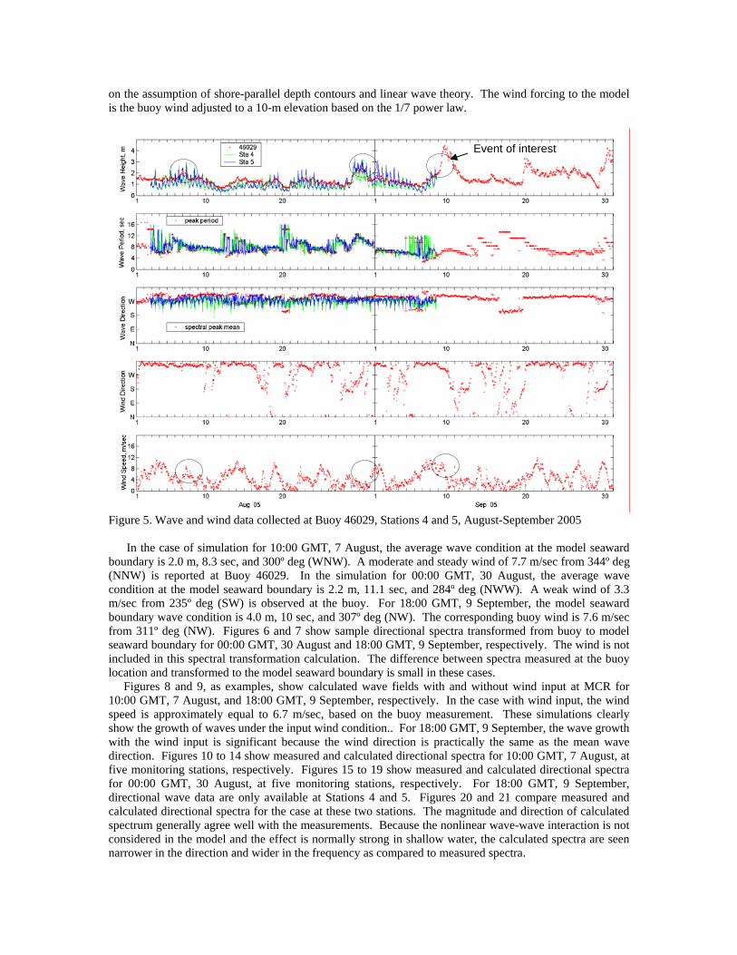
on the assumption of shore-parallel depth contours and linear wave theory. The wind forcing to the model is the buoy wind adjusted to a 10-m elevation based on the 1/7 power law.

Figure 5. Wave and wind data collected at Buoy 46029, Stations 4 and 5, August-September 2005 In the case of simulation for 10:00 GMT, 7 August, the average wave condition at the model seaward boundary is 2.0 m, 8.3 sec, and 300º deg (WNW). A moderate and steady wind of 7.7 m/sec from 344º deg (NNW) is reported at Buoy 46029. In the simulation for 00:00 GMT, 30 August, the average wave condition at the model seaward boundary is 2.2 m, 11.1 sec, and 284º deg (NWW). A weak wind of 3.3 m/sec from 235º deg (SW) is observed at the buoy. For 18:00 GMT, 9 September, the model seaward boundary wave condition is 4.0 m, 10 sec, and 307º deg (NW). The corresponding buoy wind is 7.6 m/sec from 311º deg (NW). Figures 6 and 7 show sample directional spectra transformed from buoy to model seaward boundary for 00:00 GMT, 30 August and 18:00 GMT, 9 September, respectively. The wind is not included in this spectral transformation calculation. The difference between spectra measured at the buoy location and transformed to the model seaward boundary is small in these cases. Figures 8 and 9, as examples, show calculated wave fields with and without wind input at MCR for 10:00 GMT, 7 August, and 18:00 GMT, 9 September, respectively. In the case with wind input, the wind speed is approximately equal to 6.7 m/sec, based on the buoy measurement. These simulations clearly show the growth of waves under the input wind condition.. For 18:00 GMT, 9 September, the wave growth with the wind input is significant because the wind direction is practically the same as the mean wave direction. Figures 10 to 14 show measured and calculated directional spectra for 10:00 GMT, 7 August, at five monitoring stations, respectively. Figures 15 to 19 show measured and calculated directional spectra for 00:00 GMT, 30 August, at five monitoring stations, respectively. For 18:00 GMT, 9 September, directional wave data are only available at Stations 4 and 5. Figures 20 and 21 compare measured and calculated directional spectra for the case at these two stations. The magnitude and direction of calculated spectrum generally agree well with the measurements. Because the nonlinear wave-wave interaction is not considered in the model and the effect is normally strong in shallow water, the calculated spectra are seen narrower in the direction and wider in the frequency as compared to measured spectra.

Event of interest

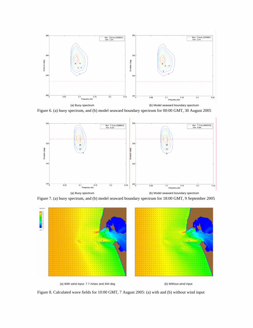
(a) Buoy spectrum (b) Model seaward boundary spectrum Figure 6. (a) buoy spectrum, and (b) model seaward boundary spectrum for 00:00 GMT, 30 August 2005

(a) Buoy spectrum (b) Model seaward boundary spectrum Figure 7. (a) buoy spectrum, and (b) model seaward boundary spectrum for 18:00 GMT, 9 September 2005

Figure 8. Calculated wave fields for 10:00 GMT, 7 August 2005: (a) with and (b) without wind input

(a) With wind input: 7.7 m/sec and 344 deg (b) Without wind input

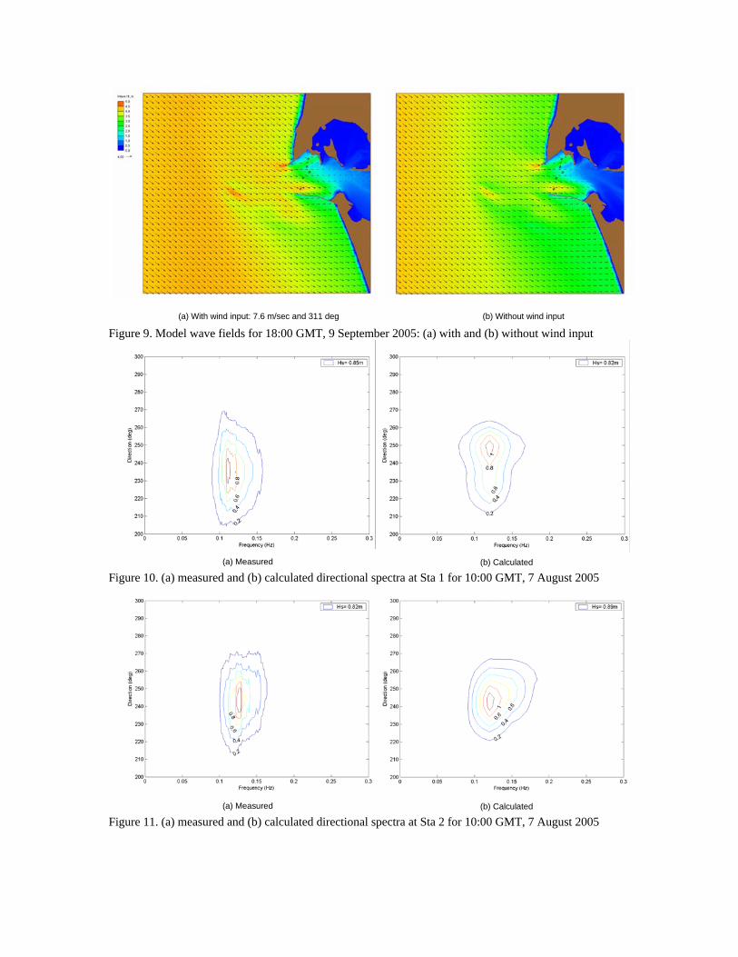
Figure 9. Model wave fields for 18:00 GMT, 9 September 2005: (a) with and (b) without wind input

(a) Measured (b) Calculated Figure 10. (a) measured and (b) calculated directional spectra at Sta 1 for 10:00 GMT, 7 August 2005


(a) With wind input: 7.6 m/sec and 311 deg (b) Without wind input









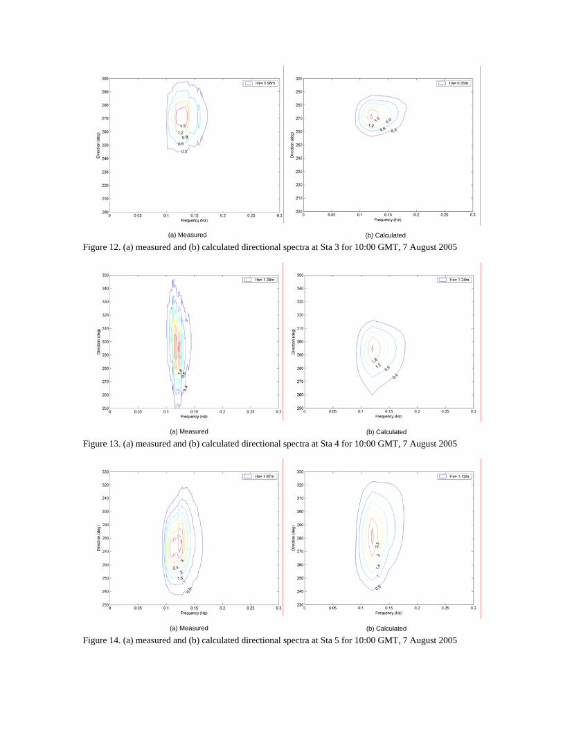
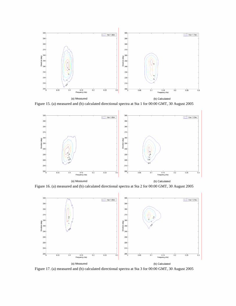
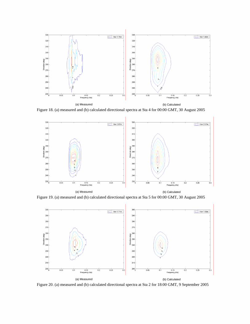
(a) Measured (b) Calculated Figure 20. (a) measured and (b) calculated directional spectra at Sta 2 for 18:00 GMT, 9 September 2005

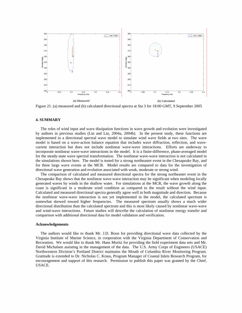
(a) Measured (b) Calculated Figure 21. (a) measured and (b) calculated directional spectra at Sta 3 for 18:00 GMT, 9 September 2005 4. SUMMARY The roles of wind input and wave dissipation functions in wave growth and evolution were investigated by authors in previous studies (Lin and Lin, 2004a, 2004b). In the present study, these functions are implemented in a directional spectral wave model to simulate wind wave fields at two sites. The wave model is based on a wave-action balance equation that includes wave diffraction, reflection, and wave-current interaction but does not include nonlinear wave-wave interactions. Efforts are underway to incorporate nonlinear wave-wave interactions in the model. It is a finite-difference, phase-averaged model for the steady-state wave spectral transformation. The nonlinear wave-wave interaction is not calculated in the simulations shown here. The model is tested for a strong northeaster event in the Chesapeake Bay, and for three large wave events at the MCR. Model results are compared to data for the investigation of directional wave generation and evolution associated with weak, moderate or strong wind. The comparison of calculated and measured directional spectra for the strong northeaster event in the Chesapeake Bay shows that the nonlinear wave-wave interaction may be significant when modeling locally generated waves by winds in the shallow water. For simulations at the MCR, the wave growth along the coast is significant in a moderate wind condition as compared to the result without the wind input. Calculated and measured directional spectra generally agree well in both magnitude and direction. Because the nonlinear wave-wave interaction is not yet implemented in the model, the calculated spectrum is somewhat skewed toward higher frequencies. The measured spectrum usually shows a much wider directional distribution than the calculated spectrum and this is most likely caused by nonlinear wave-wave and wind-wave interactions. Future studies will describe the calculation of nonlinear energy transfer and comparison with additional directional data for model validation and verification. Acknowledgements The authors would like to thank Mr. J.D. Boon for providing directional wave data collected by the Virginia Institute of Marine Science, in cooperation with the Virginia Department of Conservation and Recreation. We would like to thank Mr. Hans Moritz for providing the field experiment data sets and Mr. David Michalsen assisting in the management of the data. The U.S. Army Corps of Engineers (USACE) Northwestern Division’s Portland District maintains the Mouth of Columbia River Monitoring Program. Gratitude is extended to Dr. Nicholas C. Kraus, Program Manager of Coastal Inlets Research Program, for encouragement and support of this research. Permission to publish this paper was granted by the Chief, USACE.

References Collins, J.I. 1972. Prediction of Shallow Water Spectra, J. Geophys. Res., 77(15), 2693-2707. Hericks, D.B. and P. Osborne. 2005. Roving 3D Current Measurements across Mouth of Columbia River –Summer 2005 Oceanographic Data Collection. Pacific International Engineering, PLLC. Lin, L. and Z. Demirbilek. 2005. Evaluation of Two Numerical Wave Models with Inlet Physical Model, J. Waterway, Port, Coastal, and Ocean Engineering 131(4), 149-161. Lin, L., H. Mase, F. Yamada, and Z. Demirbilek. 2006. Wave-Action Balance Equation Diffraction (WABED) Model: Tests of Wave Diffraction and Reflection at Inlets. Technical Note, ERDC/CHL CHETN-III-73. Vicksburg, MS: U.S. Army Engineer Research and Development Center. Vicksburg, Mississippi. Lin, L. and R.-Q. Lin, 2004a. Wave Breaking Function, the 8th International Workshop on Wave Hindcasting and Prediction. North Shore, Oahu, Hawaii. November 14-19. Lin, L. and R-Q. Lin, 2006. Wave Breaking Energy in Coastal Region, the 9th International Workshop on Wave Hindcasting and Prediction. Victoria, British Columbia, Canada. September 24-29. Lin, R.-Q. and L. Lin. 2002. Using Field Buoy Data to Study Asymmetrical Wave-Wave Interactions in a Horse-Shoe Pattern, the 7th International Workshop on Wave Hindcasting and Prediction. Banff, Alberta, Canada. October 21-25. Lin, R.-Q. and L. Lin, 2004b. Wind Input Function, the 8th International Workshop on Wave Hindcasting and Prediction. North Shore, Oahu, Hawaii. November 14-19. Lin, R.-Q. and W. Perrie. 1997. A New Coast Wave Model Part III. Nonlinear Wave-Wave Interactions, J. Phys. Oceanogr., 27, 1813-1826. Lin, R.-Q. and W. Perrie. 1999. Wave-Wave Interactions in Finite Water Depth (A New Coastal Wave Model, Part IV), J. Geophys. Res., 104, No. C5, 11193-11213. Mase, H. 2001. Multi-Directional Random Wave Transformation Model Based on Energy Balance Equation, Coastal Engineering Journal 43(4), 317-337. Mase, H., K. Oki, T. Hedges, and H.J. Li. 2005. Extended Energy-Balance-Equation Wave Model for Multidirectional Random Wave Transformation,” Ocean Engineering 32, 961-985. Phillips, O. M. 1957. On the Generation of Waves by Turbulent Wind. J. Fluid Mech. 2, Part 5, 417.ne Smith, J.M., D.T. Resio, and A. Zundel. 1999. STWAVE: Steady-State Spectral Wave Model, Report 1, User’s Manual for STWAVE Version 2.0,” Instruction Report CHL-99-1, U.S. Army Engineer Waterways Experiment Station, Vicksburg, Mississippi.

Documents

Numerical Simulation of Wind Wave Field · Numerical Simulation of Wind Wave Field Lihwa Lin 1, Ray-Qing Lin 2, and Jerome P.Y. Maa3 1 U.S. Army Engineer Research and Development