computation

Article

Numerical Simulation of the Laminar ForcedConvective Heat Transfer between TwoConcentric Cylinders

Ioan Sarbu * and Anton Iosif

Department of Building Services Engineering, Polytechnic University of Timisoara, Piata Victoriei, no 2A,300006 Timisoara, Romania; anton.iosif@upt.ro* Correspondence: ioan.sarbu@upt.ro; Tel.: +40-256-403-991

Academic Editor: Demos TsahalisReceived: 20 March 2017; Accepted: 10 May 2017; Published: 13 May 2017

Abstract: The dual reciprocity method (DRM) is a highly efficient numerical method of transformingdomain integrals arising from the non-homogeneous term of the Poisson equation into equivalentboundary integrals. In this paper, the velocity and temperature fields of laminar forced heatconvection in a concentric annular tube, with constant heat flux boundary conditions, have beenstudied using numerical simulations. The DRM has been used to solve the governing equation, whichis expressed in the form of a Poisson equation. A test problem is employed to verify the DRM solutionswith different boundary element discretizations and numbers of internal points. The results of thenumerical simulations are discussed and compared with exact analytical solutions. Good agreementbetween the numerical results and exact solutions is evident, as the maximum relative errors areless than 5% to 6%, and the R2-values are greater than 0.999 in all cases. These results confirm theeffectiveness and accuracy of the proposed numerical model, which is based on the DRM.

Keywords: concentric annular tube; laminar flow; heat convection; heat flux; boundary condition;dual reciprocity method; numerical model

1. Introduction

Modern computational techniques facilitate solving problems with imposed boundary conditionsusing different numerical methods [1–9]. The numerical analysis of heat transfer [10–14] has beenindependently, though not exclusively, developed in four main streams: the finite difference method(FDM) [15,16], the finite volume method (FVM) [17], the finite element method (FEM) [18–20], andthe boundary element method (BEM) [21–23]. The FDM is based on using Taylor series expansionto find approximation formulas for derivative operators. The basic concept of the FVM is derivedfrom physical conservation laws applied to control volumes. The FDM, FVM and FEM depend on themesh that discretizes the domain via a special scheme. The FEM and BEM are based on the integralequation for heat conduction. This equation can be obtained from the differential equation using thevariational calculus.

The BEM uses a fundamental solution to convert a partial differential equation to an integralequation. In the BEM, only the boundary is discretized and an internal point’s position can be freelydefined. This method has the immediate advantage of reducing the dimensionality of the problem byone. Additionally, the BEM naturally handles the problems caused by dynamic geometry. Unlike theFEM, which requires that the domain be meshed, the BEM only discretizes the boundary. Therefore,the amount of data necessary for solving a problem can be greatly reduced [21–24]. A complete reviewof the BEM’s domain integrals is presented in [25].

Computation 2017, 5, 25; doi:10.3390/computation5020025 www.mdpi.com/journal/computation

Computation 2017, 5, 25 2 of 14

The BEM, an effective and promising numerical analysis tool due to its semi-analytical natureand ability to reduce a problem’s dimension, has been successfully applied to the homogeneouslinear heat conduction problem [26]. In the context of BEM-based velocity-vorticity formulation, thework of Žagar and Škerget [27] was one of the first attempts to solve 3D viscous laminar flow byBEM. The BEM has also been used to solve direct and inverse heat conduction problems [22,28,29].However, its extension to non-homogeneous and non-linear problems is not straightforward. Therefore,applications of the BEM to heat convection problems have not been sufficiently studied, and are still inthe development stage. Because the effects of convection are of considerable importance in many heattransfer phenomena, more research should focus on these effects. However, applying the BEM to suchproblems has drawbacks—the required fundamental solution depends on the thermal conductivity,and it is difficult to model heat generation rates (due to heat sources), because they introduce domainintegrals [30].

Several researchers have also worked on a combination of boundary element and finite elementmethods. A combined BEM-FEM model for the velocity-vorticity formulation of the Navier-Stokesequations was developed by Žunic et al. [31] to solve 3D laminar fluid flow. In the field ofviscous fluid flow numerical simulation, an important work was done by Young et al. [32] usingprimitive variable formulation of Navier-Stokes equations. They computed pressure fields withBEM and momentum equation with a three-steps FEM. In the field of viscous fluid flow numericalsimulation with velocity-vorticity formulation of Navier-Stokes equations, contributions were madeby Young et al. [33]. In their work, BEM was used to obtain boundary velocities and normal velocityfluxes implicitly, and then explicitly the internal velocities and boundary vorticities were computed byderivation of kinematical integral equations. Simulations, as well as experiments, of turbulent flowhave also been extensively investigated [34]. Hsieh and Lien [35] considered numerical modelling ofbuoyancy-driven turbulent flows in enclosures, using the Reynolds-average Navier-Stokes approach.

Recently, the radial integration method (RIM) has been developed by Gao [36], which did notrequire fundamental solutions to basis functions, and can remove various singularities appearing indomain integrals. However, although the radial integration BEM is very flexible in treating the generalnon-linear and non-homogeneous problems, the numerical evaluation of the radial integrals is verytime-consuming compared to other methods [37–39], especially for large 3D problems.

To approximate a solution to the heat conduction equation using boundary integrals, the dualreciprocity method (DRM), introduced by Nardini and Brebbia [40], can be used. The DRM preservesthe advantages of the BEM: a shorter computational time than the FEM, and a reduced number ofboundary elements. Since its introduction, the DRM has been applied to engineering problems inmany fields [41–43]. In the DRM, an available fundamental solution is used for the complete governingequation, and the domain integral arising from the heat source-like term is transferred to the boundaryusing radial interpolation functions [44–46].

In this paper, the velocity and temperature fields of laminar forced heat convection in a concentricannular tube with constant heat flux on the boundaries were studied using numerical simulations.The DRM was used to solve the governing equation, which is expressed mathematically in the form ofa Poisson equation. A test problem was employed to verify the DRM solutions with different boundaryelement discretizations and different numbers of internal points, and the results of the numericalsimulations are discussed and compared with exact analytical solutions to determine their convergenceand accuracy. A concentric annular tube was chosen because of its simplicity and ability to providean exact solution, allowing the basic nature of the proposed model for convection problems to beanalysed in detail [47,48]. Therefore, present research efforts aiming at the establishment of the DRM’sapplicability to heat convection are confirmed, and could eventually be extended to the study of otherheat transfer systems.

Computation 2017, 5, 25 3 of 14

2. Physical Problem and Its Mathematical Formulation

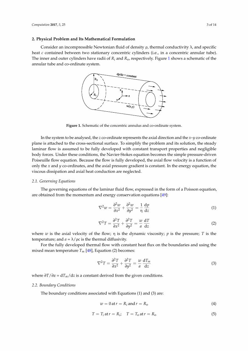
Consider an incompressible Newtonian fluid of density ρ, thermal conductivity λ, and specificheat c contained between two stationary concentric cylinders (i.e., in a concentric annular tube).The inner and outer cylinders have radii of Ri and Ro, respectively. Figure 1 shows a schematic of theannular tube and co-ordinate system.

Computation 2017, 5, 25 3 of 14

inner and outer cylinders have radii of Ri and Ro, respectively. Figure 1 shows a schematic of the

annular tube and co-ordinate system.

Figure 1. Schematic of the concentric annulus and co-ordinate system.

In the system to be analysed, the z co-ordinate represents the axial direction and the x–y

co-ordinate plane is attached to the cross-sectional surface. To simplify the problem and its solution,

the steady laminar flow is assumed to be fully developed with constant transport properties and

negligible body forces. Under these conditions, the Navier-Stokes equation becomes the simple

pressure-driven Poiseuille flow equation. Because the flow is fully developed, the axial flow velocity

is a function of only the x and y co-ordinates, and the axial pressure gradient is constant. In the

energy equation, the viscous dissipation and axial heat conduction are neglected.

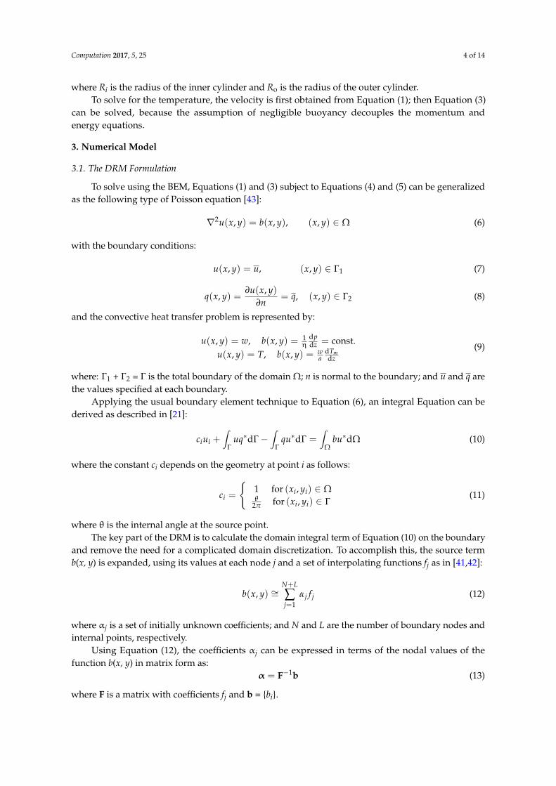
2.1. Governing Equations

The governing equations of the laminar fluid flow, expressed in the form of a Poisson equation,

are obtained from the momentum and energy conservation equations [49]:

z

p

y

w

x

ww

d

d

η

12

2

2

22

(1)

z

T

a

w

y

T

x

TT

d

d2

2

2

22

(2)

where w is the axial velocity of the flow; η is the dynamic viscosity; p is the pressure; T is the

temperature; and a = λ/ρc is the thermal diffusivity.

For the fully developed thermal flow with constant heat flux on the boundaries and using the

mixed mean temperature Tm [48], Equation (2) becomes:

z

T

a

w

y

T

x

TT m

d

d2

2

2

22

(3)

where ∂T/∂z = dTm/dz is a constant derived from the given conditions.

2.2. Boundary Conditions

The boundary conditions associated with Equations (1) and (3) are:

oandat0 RrRrw i (4)

oo at;at RrTTRrTT ii (5)

where Ri is the radius of the inner cylinder and Ro is the radius of the outer cylinder.

To solve for the temperature, the velocity is first obtained from Equation (1); then Equation (3)

can be solved, because the assumption of negligible buoyancy decouples the momentum and energy

equations.

Figure 1. Schematic of the concentric annulus and co-ordinate system.

In the system to be analysed, the z co-ordinate represents the axial direction and the x–y co-ordinateplane is attached to the cross-sectional surface. To simplify the problem and its solution, the steadylaminar flow is assumed to be fully developed with constant transport properties and negligiblebody forces. Under these conditions, the Navier-Stokes equation becomes the simple pressure-drivenPoiseuille flow equation. Because the flow is fully developed, the axial flow velocity is a function ofonly the x and y co-ordinates, and the axial pressure gradient is constant. In the energy equation, theviscous dissipation and axial heat conduction are neglected.

2.1. Governing Equations

The governing equations of the laminar fluid flow, expressed in the form of a Poisson equation,are obtained from the momentum and energy conservation equations [49]:

∇2w =∂2w∂x2 +

∂2w∂y2 =

1η

dpdz

(1)

∇2T =∂2T∂x2 +

∂2T∂y2 =

wa

dTdz

(2)

where w is the axial velocity of the flow; η is the dynamic viscosity; p is the pressure; T is thetemperature; and a = λ/ρc is the thermal diffusivity.

For the fully developed thermal flow with constant heat flux on the boundaries and using themixed mean temperature Tm [48], Equation (2) becomes:

∇2T =∂2T∂x2 +

∂2T∂y2 =

wa

dTm

dz(3)

where ∂T/∂z = dTm/dz is a constant derived from the given conditions.

2.2. Boundary Conditions

The boundary conditions associated with Equations (1) and (3) are:

w = 0 at r = Ri and r = Ro (4)

T = Ti at r = Ri; T = To at r = Ro (5)

Computation 2017, 5, 25 4 of 14

where Ri is the radius of the inner cylinder and Ro is the radius of the outer cylinder.To solve for the temperature, the velocity is first obtained from Equation (1); then Equation (3)

can be solved, because the assumption of negligible buoyancy decouples the momentum andenergy equations.

3. Numerical Model

3.1. The DRM Formulation

To solve using the BEM, Equations (1) and (3) subject to Equations (4) and (5) can be generalizedas the following type of Poisson equation [43]:

∇2u(x, y) = b(x, y), (x, y) ∈ Ω (6)

with the boundary conditions:

u(x, y) = u, (x, y) ∈ Γ1 (7)

q(x, y) =∂u(x, y)

∂n= q, (x, y) ∈ Γ2 (8)

and the convective heat transfer problem is represented by:

u(x, y) = w, b(x, y) = 1η

dpdz = const.

u(x, y) = T, b(x, y) = wa

dTmdz

(9)

where: Γ1 + Γ2 = Γ is the total boundary of the domain Ω; n is normal to the boundary; and u and q arethe values specified at each boundary.

Applying the usual boundary element technique to Equation (6), an integral Equation can bederived as described in [21]:

ciui +∫

Γuq∗dΓ−

∫Γ

qu∗dΓ =∫

Ωbu∗dΩ (10)

where the constant ci depends on the geometry at point i as follows:

ci =

1 for (xi, yi) ∈ Ωθ

2π for (xi, yi) ∈ Γ(11)

where θ is the internal angle at the source point.The key part of the DRM is to calculate the domain integral term of Equation (10) on the boundary

and remove the need for a complicated domain discretization. To accomplish this, the source termb(x, y) is expanded, using its values at each node j and a set of interpolating functions fj as in [41,42]:

b(x, y) ∼=N+L

∑j=1

αj f j (12)

where αj is a set of initially unknown coefficients; and N and L are the number of boundary nodes andinternal points, respectively.

Using Equation (12), the coefficients αj can be expressed in terms of the nodal values of thefunction b(x, y) in matrix form as:

α = F−1b (13)

where F is a matrix with coefficients fj and b = bi.

Computation 2017, 5, 25 5 of 14

The radial basis functions fj are linked with the particular solutions uj to the equation:

∇2uj = f j (14)

Substituting Equation (14) into Equation (12) and applying integration by parts to the domainintegral term of Equation (10) twice leads to:

ciui +∫

Γuq∗dΓ−

∫Γ

qu∗dΓ =N+L

∑j=1

αj

(ciuij +

∫Γ

ujq∗dΓ−∫

Γqju∗dΓ

)(15)

On a two-dimensional domain, u∗, q∗ and u, q can be derived as:

u∗ =1

2πln(

1r); q∗ =

−12π r∇r ·→n (16)

u =r2

4+

r3

9; q = (

r2+

r2

3)∇r ·→n (17)

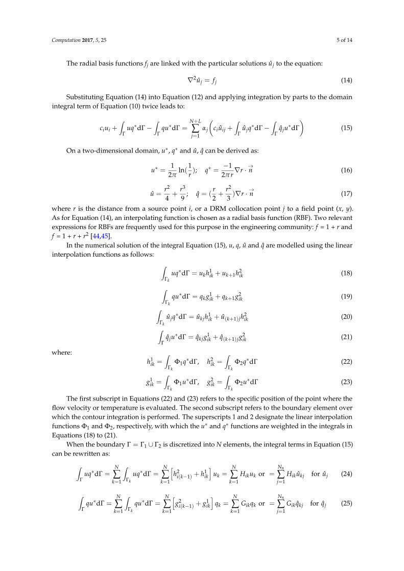
where r is the distance from a source point i, or a DRM collocation point j to a field point (x, y).As for Equation (14), an interpolating function is chosen as a radial basis function (RBF). Two relevantexpressions for RBFs are frequently used for this purpose in the engineering community: f = 1 + r andf = 1 + r + r2 [44,45].

In the numerical solution of the integral Equation (15), u, q, u and q are modelled using the linearinterpolation functions as follows: ∫

Γk

uq∗dΓ = ukh1ik + uk+1h2

ik (18)

∫Γk

qu∗dΓ = qkg1ik + qk+1g2

ik (19)

∫Γk

ujq∗dΓ = ukjh1ik + u(k+1)jh

2ik (20)

∫Γ

qju∗dΓ = qkjg1ik + q(k+1)jg

2ik (21)

where:h1

ik =∫

Γk

Φ1q∗dΓ, h2ik =

∫Γk

Φ2q∗dΓ (22)

g1ik =

∫Γk

Φ1u∗dΓ, g2ik =

∫Γk

Φ2u∗dΓ (23)

The first subscript in Equations (22) and (23) refers to the specific position of the point where theflow velocity or temperature is evaluated. The second subscript refers to the boundary element overwhich the contour integration is performed. The superscripts 1 and 2 designate the linear interpolationfunctions Φ1 and Φ2, respectively, with which the u∗ and q∗ functions are weighted in the integrals inEquations (18) to (21).

When the boundary Γ = Γ1 ∪ Γ2 is discretized into N elements, the integral terms in Equation (15)can be rewritten as:

∫Γ

uq∗dΓ =N

∑k=1

∫Γk

uq∗dΓ =N

∑k=1

[h2

i(k−1) + h1ik

]uk =

N

∑k=1

Hikuk or =Nn

∑j=1

Hikukj for uj (24)

∫Γ

qu∗dΓ =N

∑k=1

∫Γk

qu∗dΓ =N

∑k=1

[g2

i(k−1) + g1ik

]qk =

N

∑k=1

Gikqk or =Nn

∑j=1

Gik qkj for qj (25)

Computation 2017, 5, 25 6 of 14

where h2i0 = h2

iN and g2i0 = g2

iN .Substituting Equations (24) and (25) into Equation (15), after several manipulations, yields the

dual reciprocity boundary element Equation:

ciui +N

∑k=1

Hikuk −N

∑k=1

Gikqk =N+L

∑j=1

αj

(ciuij +

N

∑k=1

Hikukj −N

∑k=1

Gik qkj

)(26)

3.2. Numerical Solution

Equation (26) can now be written in a matrix-vector form as:

HU−GQ = (HU−GQ)α (27)

where H and G are matrices with elements Hik and Gik, with ci incorporated into the principal diagonalelement; and U, Q and their terms U, Q correspond to vectors with elements uk and qk, and matriceswith ukj and qkj as the jth column vectors.

Substituting α from Equation (13) into the above equation yields:

HU−GQ = (HU−GQ)F−1b (28)

Introducing the boundary conditions into the nodes of the uk and qk vectors, and rearranging bymoving known quantities to the right-hand side and unknown quantities to the left-hand side, leads toa system of linear equations of the form:

AX = B (29)

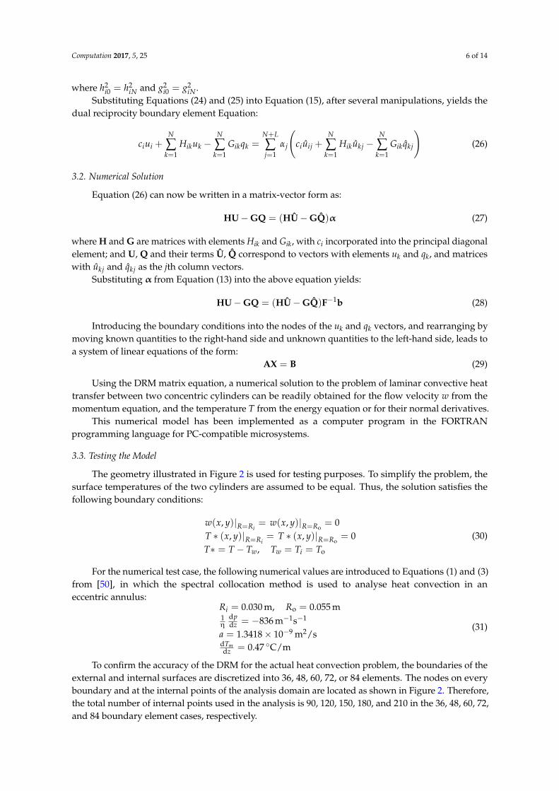
Using the DRM matrix equation, a numerical solution to the problem of laminar convective heattransfer between two concentric cylinders can be readily obtained for the flow velocity w from themomentum equation, and the temperature T from the energy equation or for their normal derivatives.

This numerical model has been implemented as a computer program in the FORTRANprogramming language for PC-compatible microsystems.

3.3. Testing the Model

The geometry illustrated in Figure 2 is used for testing purposes. To simplify the problem, thesurface temperatures of the two cylinders are assumed to be equal. Thus, the solution satisfies thefollowing boundary conditions:

w(x, y)|R=Ri= w(x, y)|R=Ro

= 0T ∗ (x, y)|R=Ri

= T ∗ (x, y)|R=Ro= 0

T∗ = T − Tw, Tw = Ti = To

(30)

For the numerical test case, the following numerical values are introduced to Equations (1) and (3)from [50], in which the spectral collocation method is used to analyse heat convection in aneccentric annulus:

Ri = 0.030 m, Ro = 0.055 m1η

dpdz = −836 m−1s−1

a = 1.3418× 10−9 m2/sdTmdz = 0.47 C/m

(31)

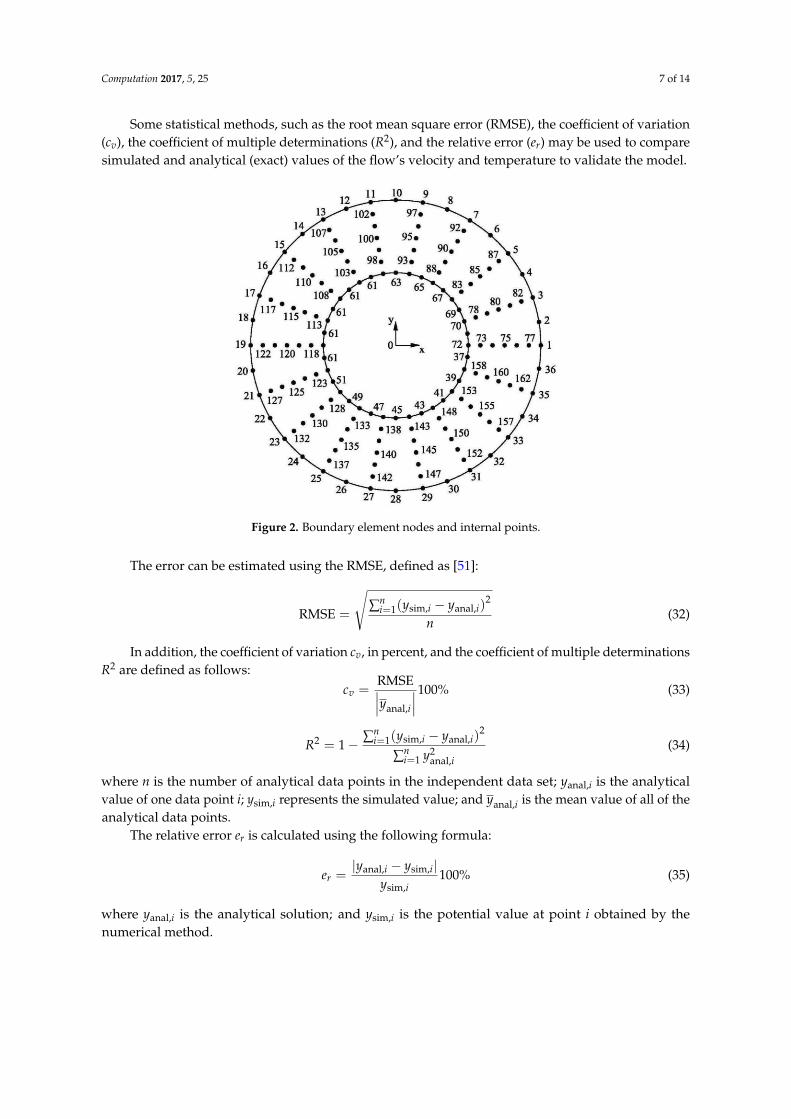
To confirm the accuracy of the DRM for the actual heat convection problem, the boundaries of theexternal and internal surfaces are discretized into 36, 48, 60, 72, or 84 elements. The nodes on everyboundary and at the internal points of the analysis domain are located as shown in Figure 2. Therefore,the total number of internal points used in the analysis is 90, 120, 150, 180, and 210 in the 36, 48, 60, 72,and 84 boundary element cases, respectively.

Computation 2017, 5, 25 7 of 14

Some statistical methods, such as the root mean square error (RMSE), the coefficient of variation(cv), the coefficient of multiple determinations (R2), and the relative error (er) may be used to comparesimulated and analytical (exact) values of the flow’s velocity and temperature to validate the model.Computation 2017, 5, 25 7 of 14

Figure 2. Boundary element nodes and internal points.

The error can be estimated using the RMSE, defined as [51]:

n

yyn

iii

1

2

,anal,sim

RMSE (32)

In addition, the coefficient of variation cv, in percent, and the coefficient of multiple

determinations R2 are defined as follows:

%100RMSE

,anal i

vy

c (33)

n

ii

n

iii

y

yyR

1

2

,anal

1

2

,anal,sim2 1 (34)

where n is the number of analytical data points in the independent data set; yanal,i is the analytical

value of one data point i; ysim,i represents the simulated value; and iy ,anal is the mean value of all of

the analytical data points.

The relative error er is calculated using the following formula:

%100,sim

,sim,anal

i

ii

ry

yye

(35)

where yanal,i is the analytical solution; and ysim,i is the potential value at point i obtained by the

numerical method.

4. Simulation Results and Discussion

To obtain the axial flow velocity w (x, y), Equation (1) is solved first. The results for the

boundary and internal nodes are shown in Tables 1 and 2 for the RBFs f = 1 + r and f = 1 + r + r2,

respectively. In these tables, the normal derivative of the velocity w at the boundary is also listed,

and all of the numerical solutions are compared with the exact solutions [47], in order to determine

their accuracy. In addition, statistical values such as the RMSE, cv, and R2, which correspond to

different numbers of boundary elements in the analysed system, are given in Tables 1 and 2.

Figure 2. Boundary element nodes and internal points.

The error can be estimated using the RMSE, defined as [51]:

RMSE =

√∑n

i=1(ysim,i − yanal,i)2

n(32)

In addition, the coefficient of variation cv, in percent, and the coefficient of multiple determinationsR2 are defined as follows:

cv =RMSE∣∣∣yanal,i

∣∣∣100% (33)

R2 = 1− ∑ni=1(ysim,i − yanal,i)

2

∑ni=1 y2

anal,i(34)

where n is the number of analytical data points in the independent data set; yanal,i is the analyticalvalue of one data point i; ysim,i represents the simulated value; and yanal,i is the mean value of all of theanalytical data points.

The relative error er is calculated using the following formula:

er =|yanal,i − ysim,i|

ysim,i100% (35)

where yanal,i is the analytical solution; and ysim,i is the potential value at point i obtained by thenumerical method.

Computation 2017, 5, 25 8 of 14

4. Simulation Results and Discussion

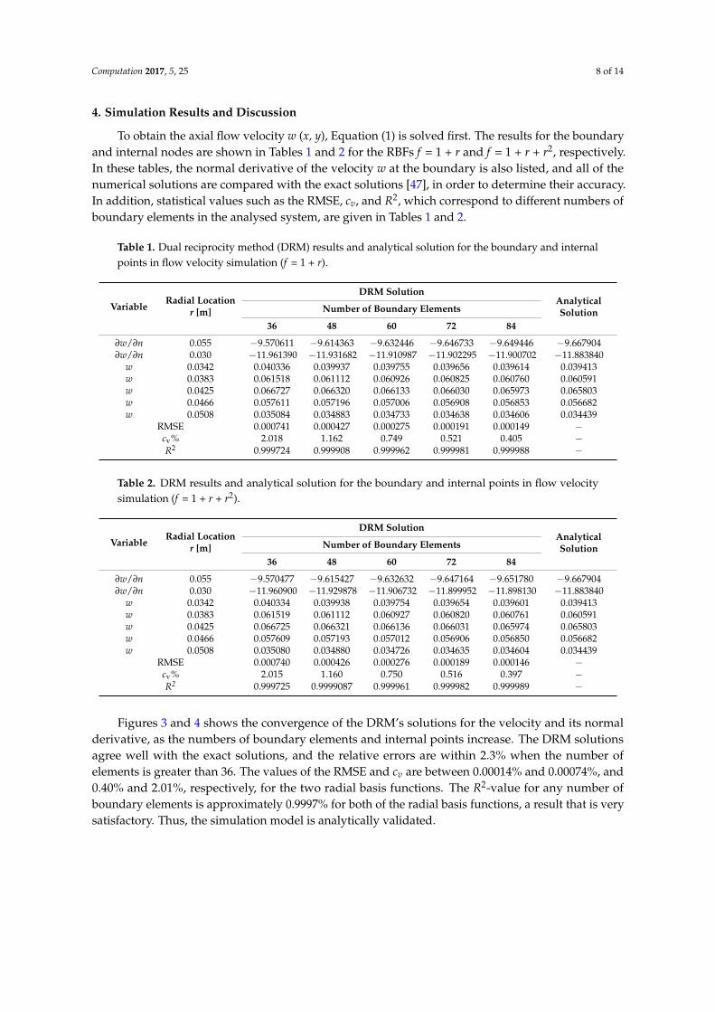
To obtain the axial flow velocity w (x, y), Equation (1) is solved first. The results for the boundaryand internal nodes are shown in Tables 1 and 2 for the RBFs f = 1 + r and f = 1 + r + r2, respectively.In these tables, the normal derivative of the velocity w at the boundary is also listed, and all of thenumerical solutions are compared with the exact solutions [47], in order to determine their accuracy.In addition, statistical values such as the RMSE, cv, and R2, which correspond to different numbers ofboundary elements in the analysed system, are given in Tables 1 and 2.

Table 1. Dual reciprocity method (DRM) results and analytical solution for the boundary and internalpoints in flow velocity simulation (f = 1 + r).

VariableRadial Location

r [m]

DRM SolutionAnalyticalSolutionNumber of Boundary Elements

36 48 60 72 84

∂w/∂n 0.055 −9.570611 −9.614363 −9.632446 −9.646733 −9.649446 −9.667904∂w/∂n 0.030 −11.961390 −11.931682 −11.910987 −11.902295 −11.900702 −11.883840

w 0.0342 0.040336 0.039937 0.039755 0.039656 0.039614 0.039413w 0.0383 0.061518 0.061112 0.060926 0.060825 0.060760 0.060591w 0.0425 0.066727 0.066320 0.066133 0.066030 0.065973 0.065803w 0.0466 0.057611 0.057196 0.057006 0.056908 0.056853 0.056682w 0.0508 0.035084 0.034883 0.034733 0.034638 0.034606 0.034439

RMSE 0.000741 0.000427 0.000275 0.000191 0.000149 −cv% 2.018 1.162 0.749 0.521 0.405 −R2 0.999724 0.999908 0.999962 0.999981 0.999988 −

Table 2. DRM results and analytical solution for the boundary and internal points in flow velocitysimulation (f = 1 + r + r2).

VariableRadial Location

r [m]

DRM SolutionAnalyticalSolutionNumber of Boundary Elements

36 48 60 72 84

∂w/∂n 0.055 −9.570477 −9.615427 −9.632632 −9.647164 −9.651780 −9.667904∂w/∂n 0.030 −11.960900 −11.929878 −11.906732 −11.899952 −11.898130 −11.883840

w 0.0342 0.040334 0.039938 0.039754 0.039654 0.039601 0.039413w 0.0383 0.061519 0.061112 0.060927 0.060820 0.060761 0.060591w 0.0425 0.066725 0.066321 0.066136 0.066031 0.065974 0.065803w 0.0466 0.057609 0.057193 0.057012 0.056906 0.056850 0.056682w 0.0508 0.035080 0.034880 0.034726 0.034635 0.034604 0.034439

RMSE 0.000740 0.000426 0.000276 0.000189 0.000146 −cv% 2.015 1.160 0.750 0.516 0.397 −R2 0.999725 0.9999087 0.999961 0.999982 0.999989 −

Figures 3 and 4 shows the convergence of the DRM’s solutions for the velocity and its normalderivative, as the numbers of boundary elements and internal points increase. The DRM solutionsagree well with the exact solutions, and the relative errors are within 2.3% when the number ofelements is greater than 36. The values of the RMSE and cv are between 0.00014% and 0.00074%, and0.40% and 2.01%, respectively, for the two radial basis functions. The R2-value for any number ofboundary elements is approximately 0.9997% for both of the radial basis functions, a result that is verysatisfactory. Thus, the simulation model is analytically validated.

Computation 2017, 5, 25 9 of 14

Computation 2017, 5, 25 8 of 14

Table 1. Dual reciprocity method (DRM) results and analytical solution for the boundary and

internal points in flow velocity simulation (f = 1 + r).

Variable Radial Location

r [m]

DRM Solution Analytical

Solution Number of Boundary Elements

36 48 60 72 84

∂w/∂n 0.055 −9.570611 −9.614363 −9.632446 −9.646733 −9.649446 −9.667904

∂w/∂n 0.030 −11.961390 −11.931682 −11.910987 −11.902295 −11.900702 −11.883840

w 0.0342 0.040336 0.039937 0.039755 0.039656 0.039614 0.039413

w 0.0383 0.061518 0.061112 0.060926 0.060825 0.060760 0.060591

w 0.0425 0.066727 0.066320 0.066133 0.066030 0.065973 0.065803

w 0.0466 0.057611 0.057196 0.057006 0.056908 0.056853 0.056682

w 0.0508 0.035084 0.034883 0.034733 0.034638 0.034606 0.034439

RMSE 0.000741 0.000427 0.000275 0.000191 0.000149 −

cv% 2.018 1.162 0.749 0.521 0.405 −

R2 0.999724 0.999908 0.999962 0.999981 0.999988 −

Table 2. DRM results and analytical solution for the boundary and internal points in flow velocity

simulation (f = 1 + r + r2).

Variable Radial Location

r [m]

DRM Solution Analytical

Solution Number of Boundary Elements

36 48 60 72 84

∂w/∂n 0.055 −9.570477 −9.615427 −9.632632 −9.647164 −9.651780 −9.667904

∂w/∂n 0.030 −11.960900 −11.929878 −11.906732 −11.899952 −11.898130 −11.883840

w 0.0342 0.040334 0.039938 0.039754 0.039654 0.039601 0.039413

w 0.0383 0.061519 0.061112 0.060927 0.060820 0.060761 0.060591

w 0.0425 0.066725 0.066321 0.066136 0.066031 0.065974 0.065803

w 0.0466 0.057609 0.057193 0.057012 0.056906 0.056850 0.056682

w 0.0508 0.035080 0.034880 0.034726 0.034635 0.034604 0.034439

RMSE 0.000740 0.000426 0.000276 0.000189 0.000146 −

cv% 2.015 1.160 0.750 0.516 0.397 −

R2 0.999725 0.9999087 0.999961 0.999982 0.999989 −

Figures 3 and 4 shows the convergence of the DRM’s solutions for the velocity and its normal

derivative, as the numbers of boundary elements and internal points increase. The DRM solutions

agree well with the exact solutions, and the relative errors are within 2.3% when the number of

elements is greater than 36. The values of the RMSE and cv are between 0.00014% and 0.00074%, and

0.40% and 2.01%, respectively, for the two radial basis functions. The R2-value for any number of

boundary elements is approximately 0.9997% for both of the radial basis functions, a result that is

very satisfactory. Thus, the simulation model is analytically validated.

(a) (b)

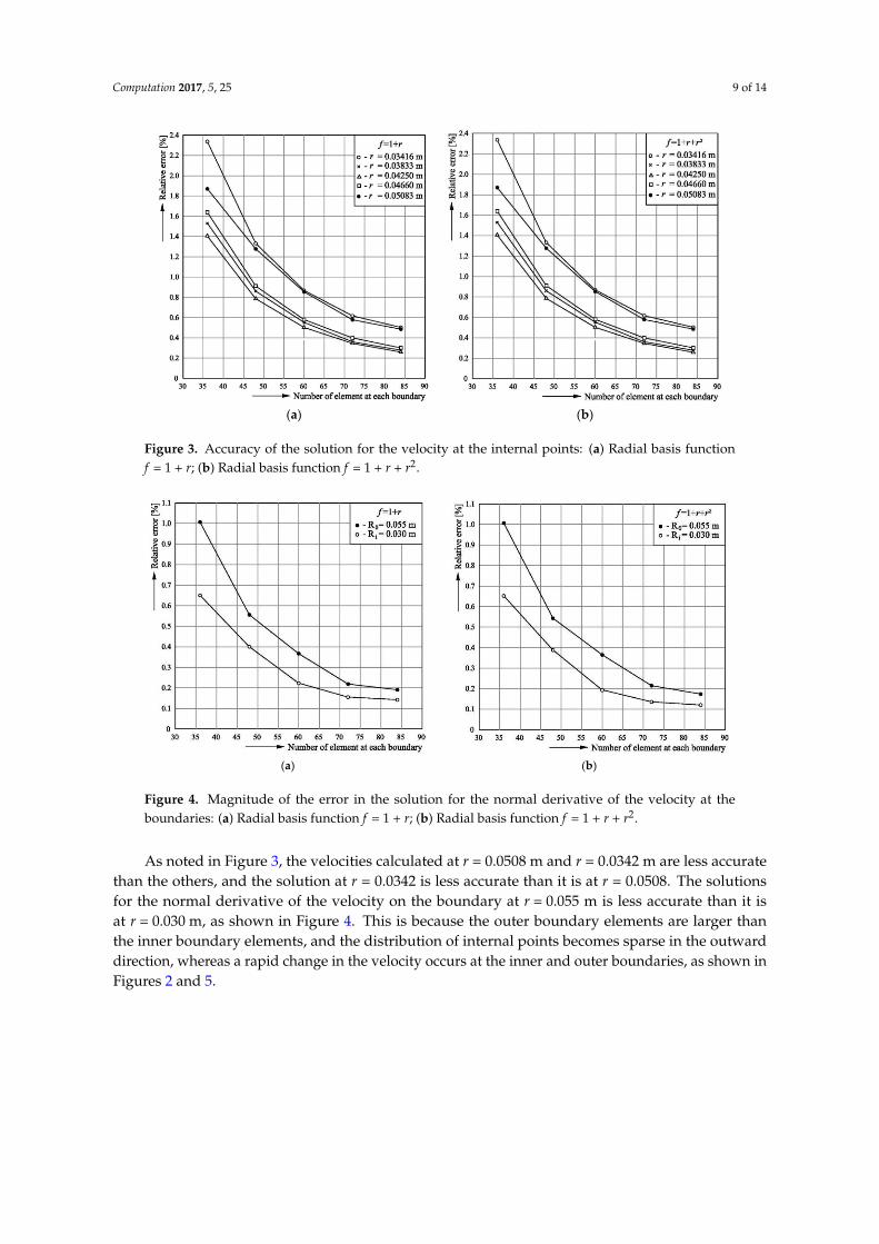
Figure 3. Accuracy of the solution for the velocity at the internal points: (a) Radial basis function f = 1

+ r; (b) Radial basis function f = 1 + r + r2. Figure 3. Accuracy of the solution for the velocity at the internal points: (a) Radial basis functionf = 1 + r; (b) Radial basis function f = 1 + r + r2.Computation 2017, 5, 25 9 of 14

(a) (b)

Figure 4. Magnitude of the error in the solution for the normal derivative of the velocity at the

boundaries: (a) Radial basis function f = 1 + r; (b) Radial basis function f = 1 + r + r2.

As noted in Figure 3, the velocities calculated at r = 0.0508 m and r = 0.0342 m are less accurate

than the others, and the solution at r = 0.0342 is less accurate than it is at r = 0.0508. The solutions for

the normal derivative of the velocity on the boundary at r = 0.055 m is less accurate than it is at r =

0.030 m, as shown in Figure 4. This is because the outer boundary elements are larger than the inner

boundary elements, and the distribution of internal points becomes sparse in the outward direction,

whereas a rapid change in the velocity occurs at the inner and outer boundaries, as shown in Figures

2 and 5.

(a) (b)

Figure 5. Comparison of velocity profile obtained using analytical solution and DRM results: (a)

Radial basis function f = 1 + r; (b) Radial basis function f = 1 + r + r2.

Therefore, the magnitude of the solution’s error in the radial direction is closely related to the

physical and the mathematical aspects of the problem; hence, the overall accuracy of the solution is

fairly acceptable. Therefore, when 36 elements are used, the solution has a maximum error of 2.34%

at radial position r = 0.0342 m, and the next step results in an accurate solution for the temperature.

The DRM solutions for the velocity are, in turn, used in the energy equation (Equation (3)) to solve

for the temperature distribution. Tables 3 and 4 show the simulation results for temperature and

statistical values such as the RMSE, cv, and R2. The DRM solutions are in excellent agreement with

the exact solutions and the relative errors er are within 5% when 36 elements are used (Figures 6–8).

The cv values are in the range of 0.3%–5.0%, and the R2-value is approximately 0.999 for the two

Figure 4. Magnitude of the error in the solution for the normal derivative of the velocity at theboundaries: (a) Radial basis function f = 1 + r; (b) Radial basis function f = 1 + r + r2.

As noted in Figure 3, the velocities calculated at r = 0.0508 m and r = 0.0342 m are less accuratethan the others, and the solution at r = 0.0342 is less accurate than it is at r = 0.0508. The solutionsfor the normal derivative of the velocity on the boundary at r = 0.055 m is less accurate than it isat r = 0.030 m, as shown in Figure 4. This is because the outer boundary elements are larger thanthe inner boundary elements, and the distribution of internal points becomes sparse in the outwarddirection, whereas a rapid change in the velocity occurs at the inner and outer boundaries, as shown inFigures 2 and 5.

Computation 2017, 5, 25 10 of 14

Computation 2017, 5, 25 9 of 14

(a) (b)

Figure 4. Magnitude of the error in the solution for the normal derivative of the velocity at the

boundaries: (a) Radial basis function f = 1 + r; (b) Radial basis function f = 1 + r + r2.

As noted in Figure 3, the velocities calculated at r = 0.0508 m and r = 0.0342 m are less accurate

than the others, and the solution at r = 0.0342 is less accurate than it is at r = 0.0508. The solutions for

the normal derivative of the velocity on the boundary at r = 0.055 m is less accurate than it is at r =

0.030 m, as shown in Figure 4. This is because the outer boundary elements are larger than the inner

boundary elements, and the distribution of internal points becomes sparse in the outward direction,

whereas a rapid change in the velocity occurs at the inner and outer boundaries, as shown in Figures

2 and 5.

(a) (b)

Figure 5. Comparison of velocity profile obtained using analytical solution and DRM results: (a)

Radial basis function f = 1 + r; (b) Radial basis function f = 1 + r + r2.

Therefore, the magnitude of the solution’s error in the radial direction is closely related to the

physical and the mathematical aspects of the problem; hence, the overall accuracy of the solution is

fairly acceptable. Therefore, when 36 elements are used, the solution has a maximum error of 2.34%

at radial position r = 0.0342 m, and the next step results in an accurate solution for the temperature.

The DRM solutions for the velocity are, in turn, used in the energy equation (Equation (3)) to solve

for the temperature distribution. Tables 3 and 4 show the simulation results for temperature and

statistical values such as the RMSE, cv, and R2. The DRM solutions are in excellent agreement with

the exact solutions and the relative errors er are within 5% when 36 elements are used (Figures 6–8).

The cv values are in the range of 0.3%–5.0%, and the R2-value is approximately 0.999 for the two

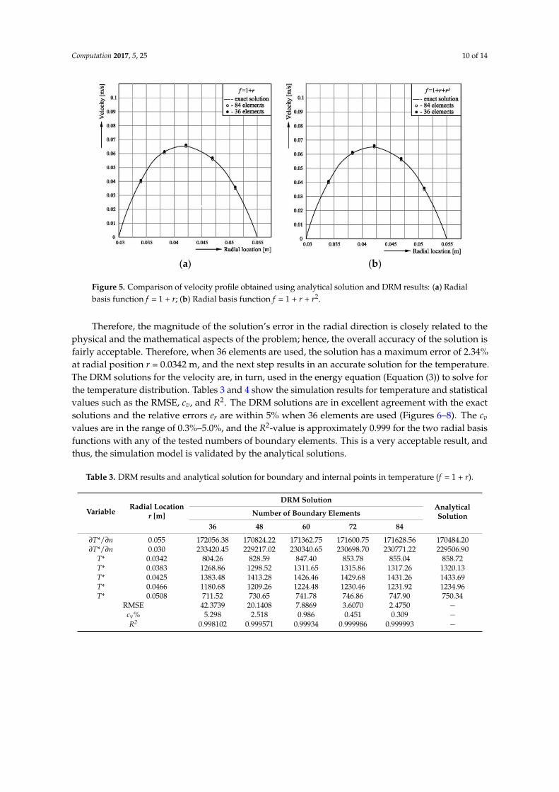
Figure 5. Comparison of velocity profile obtained using analytical solution and DRM results: (a) Radialbasis function f = 1 + r; (b) Radial basis function f = 1 + r + r2.

Therefore, the magnitude of the solution’s error in the radial direction is closely related to thephysical and the mathematical aspects of the problem; hence, the overall accuracy of the solution isfairly acceptable. Therefore, when 36 elements are used, the solution has a maximum error of 2.34%at radial position r = 0.0342 m, and the next step results in an accurate solution for the temperature.The DRM solutions for the velocity are, in turn, used in the energy equation (Equation (3)) to solve forthe temperature distribution. Tables 3 and 4 show the simulation results for temperature and statisticalvalues such as the RMSE, cv, and R2. The DRM solutions are in excellent agreement with the exactsolutions and the relative errors er are within 5% when 36 elements are used (Figures 6–8). The cv

values are in the range of 0.3%–5.0%, and the R2-value is approximately 0.999 for the two radial basisfunctions with any of the tested numbers of boundary elements. This is a very acceptable result, andthus, the simulation model is validated by the analytical solutions.

Table 3. DRM results and analytical solution for boundary and internal points in temperature (f = 1 + r).

VariableRadial Location

r [m]

DRM SolutionAnalyticalSolutionNumber of Boundary Elements

36 48 60 72 84

∂T*/∂n 0.055 172056.38 170824.22 171362.75 171600.75 171628.56 170484.20∂T*/∂n 0.030 233420.45 229217.02 230340.65 230698.70 230771.22 229506.90

T* 0.0342 804.26 828.59 847.40 853.78 855.04 858.72T* 0.0383 1268.86 1298.52 1311.65 1315.86 1317.26 1320.13T* 0.0425 1383.48 1413.28 1426.46 1429.68 1431.26 1433.69T* 0.0466 1180.68 1209.26 1224.48 1230.46 1231.92 1234.96T* 0.0508 711.52 730.65 741.78 746.86 747.90 750.34

RMSE 42.3739 20.1408 7.8869 3.6070 2.4750 −cv% 5.298 2.518 0.986 0.451 0.309 −R2 0.998102 0.999571 0.99934 0.999986 0.999993 −

Computation 2017, 5, 25 11 of 14

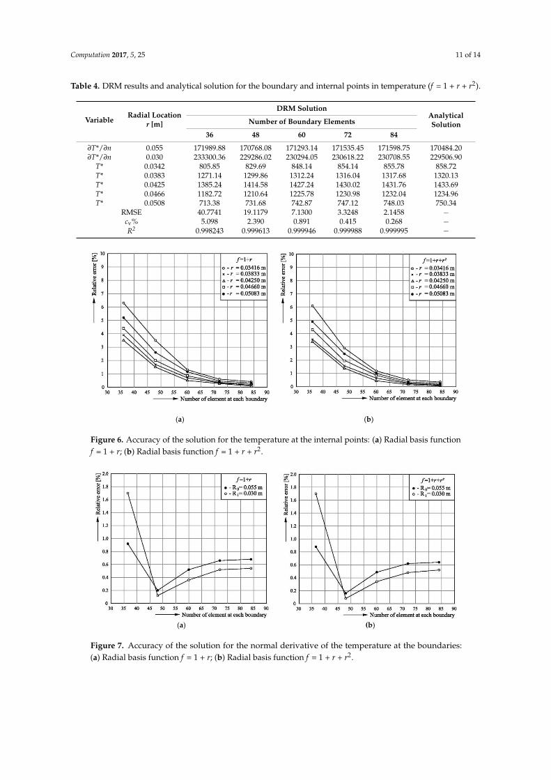
Table 4. DRM results and analytical solution for the boundary and internal points in temperature (f = 1 + r + r2).

VariableRadial Location

r [m]

DRM SolutionAnalyticalSolutionNumber of Boundary Elements

36 48 60 72 84

∂T*/∂n 0.055 171989.88 170768.08 171293.14 171535.45 171598.75 170484.20∂T*/∂n 0.030 233300.36 229286.02 230294.05 230618.22 230708.55 229506.90

T* 0.0342 805.85 829.69 848.14 854.14 855.78 858.72T* 0.0383 1271.14 1299.86 1312.24 1316.04 1317.68 1320.13T* 0.0425 1385.24 1414.58 1427.24 1430.02 1431.76 1433.69T* 0.0466 1182.72 1210.64 1225.78 1230.98 1232.04 1234.96T* 0.0508 713.38 731.68 742.87 747.12 748.03 750.34

RMSE 40.7741 19.1179 7.1300 3.3248 2.1458 −cv% 5.098 2.390 0.891 0.415 0.268 −R2 0.998243 0.999613 0.999946 0.999988 0.999995 −

Computation 2017, 5, 25 10 of 14

radial basis functions with any of the tested numbers of boundary elements. This is a very acceptable

result, and thus, the simulation model is validated by the analytical solutions.

Table 3. DRM results and analytical solution for boundary and internal points in temperature (f = 1 + r).

Variable Radial Location

r [m]

DRM Solution

Analytical Solution Number of Boundary Elements

36 48 60 72 84

∂T*/∂n 0.055 172056.38 170824.22 171362.75 171600.75 171628.56 170484.20

∂T*/∂n 0.030 233420.45 229217.02 230340.65 230698.70 230771.22 229506.90

T* 0.0342 804.26 828.59 847.40 853.78 855.04 858.72

T* 0.0383 1268.86 1298.52 1311.65 1315.86 1317.26 1320.13

T* 0.0425 1383.48 1413.28 1426.46 1429.68 1431.26 1433.69

T* 0.0466 1180.68 1209.26 1224.48 1230.46 1231.92 1234.96

T* 0.0508 711.52 730.65 741.78 746.86 747.90 750.34

RMSE 42.3739 20.1408 7.8869 3.6070 2.4750 −

cv% 5.298 2.518 0.986 0.451 0.309 −

R2 0.998102 0.999571 0.99934 0.999986 0.999993 −

Table 4. DRM results and analytical solution for the boundary and internal points in temperature

(f = 1 + r + r2).

Variable

Radial

Location

r [m]

DRM Solution Analytical

Solution Number of Boundary Elements

36 48 60 72 84

∂T*/∂n 0.055 171989.88 170768.08 171293.14 171535.4

5

171598.7

5 170484.20

∂T*/∂n 0.030 233300.36 229286.02 230294.05 230618.2

2

230708.5

5 229506.90

T* 0.0342 805.85 829.69 848.14 854.14 855.78 858.72

T* 0.0383 1271.14 1299.86 1312.24 1316.04 1317.68 1320.13

T* 0.0425 1385.24 1414.58 1427.24 1430.02 1431.76 1433.69

T* 0.0466 1182.72 1210.64 1225.78 1230.98 1232.04 1234.96

T* 0.0508 713.38 731.68 742.87 747.12 748.03 750.34

RMSE 40.7741 19.1179 7.1300 3.3248 2.1458 −

cv% 5.098 2.390 0.891 0.415 0.268 −

R2 0.998243 0.999613 0.999946 0.999988 0.999995 −

(a) (b)

Figure 6. Accuracy of the solution for the temperature at the internal points: (a) Radial basis function

f = 1 + r; (b) Radial basis function f = 1 + r + r2. Figure 6. Accuracy of the solution for the temperature at the internal points: (a) Radial basis functionf = 1 + r; (b) Radial basis function f = 1 + r + r2.Computation 2017, 5, 25 11 of 14

(a) (b)

Figure 7. Accuracy of the solution for the normal derivative of the temperature at the boundaries: (a)

Radial basis function f = 1 + r; (b) Radial basis function f = 1 + r + r2.

(a) (b)

Figure 8. Comparison of temperature profile T* obtained using analytical solution and DRM results:

(a) Radial basis function f= 1 + r; (b) Radial basis function f = 1 + r + r2.

Although the convergence trend shown in Figure 7 is not monotonic and the radial location’s

effect on the magnitude of the error does not exactly follow the trend shown in the previous case, the

solution trends can be considered indistinguishable within 1% relative error.

These test results validate the power of the dual reciprocity boundary element method and the

accuracy of its solutions. This is because the numerical solution for the velocity was used as an input

in Equation (3), and the source-like function b(x, y) of Equation (12) in Equation (3) was

approximated using interpolating functions and the nodal values of internal points.

As a final note, all of the numbers of elements tested are adequate for solving this problem. The

amount of error in the solutions for the velocity and temperature is acceptable. Using the

fourth-order RBFs, the accuracy of the DRM is increased insignificantly, so that only minor

differences are observed between errors (0.2%). The errors can be decreased using only a higher

adequate number of boundary elements and internal points limited by computational capacity.

5. Conclusions

A numerical simulation model based on the dual reciprocity boundary element method has

been developed for the solution of the laminar heat convection problem between two concentric

cylinders with a constant imposed heat flux.

Figure 7. Accuracy of the solution for the normal derivative of the temperature at the boundaries:(a) Radial basis function f = 1 + r; (b) Radial basis function f = 1 + r + r2.

Computation 2017, 5, 25 12 of 14

Computation 2017, 5, 25 11 of 14

(a) (b)

Figure 7. Accuracy of the solution for the normal derivative of the temperature at the boundaries: (a)

Radial basis function f = 1 + r; (b) Radial basis function f = 1 + r + r2.

(a) (b)

Figure 8. Comparison of temperature profile T* obtained using analytical solution and DRM results:

(a) Radial basis function f= 1 + r; (b) Radial basis function f = 1 + r + r2.

Although the convergence trend shown in Figure 7 is not monotonic and the radial location’s

effect on the magnitude of the error does not exactly follow the trend shown in the previous case, the

solution trends can be considered indistinguishable within 1% relative error.

These test results validate the power of the dual reciprocity boundary element method and the

accuracy of its solutions. This is because the numerical solution for the velocity was used as an input

in Equation (3), and the source-like function b(x, y) of Equation (12) in Equation (3) was

approximated using interpolating functions and the nodal values of internal points.

As a final note, all of the numbers of elements tested are adequate for solving this problem. The

amount of error in the solutions for the velocity and temperature is acceptable. Using the

fourth-order RBFs, the accuracy of the DRM is increased insignificantly, so that only minor

differences are observed between errors (0.2%). The errors can be decreased using only a higher

adequate number of boundary elements and internal points limited by computational capacity.

5. Conclusions

A numerical simulation model based on the dual reciprocity boundary element method has

been developed for the solution of the laminar heat convection problem between two concentric

cylinders with a constant imposed heat flux.

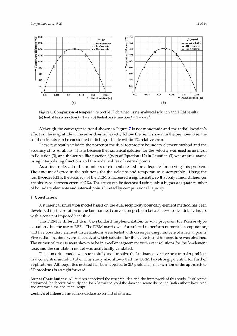
Figure 8. Comparison of temperature profile T* obtained using analytical solution and DRM results:(a) Radial basis function f = 1 + r; (b) Radial basis function f = 1 + r + r2.

Although the convergence trend shown in Figure 7 is not monotonic and the radial location’seffect on the magnitude of the error does not exactly follow the trend shown in the previous case, thesolution trends can be considered indistinguishable within 1% relative error.

These test results validate the power of the dual reciprocity boundary element method and theaccuracy of its solutions. This is because the numerical solution for the velocity was used as an inputin Equation (3), and the source-like function b(x, y) of Equation (12) in Equation (3) was approximatedusing interpolating functions and the nodal values of internal points.

As a final note, all of the numbers of elements tested are adequate for solving this problem.The amount of error in the solutions for the velocity and temperature is acceptable. Using thefourth-order RBFs, the accuracy of the DRM is increased insignificantly, so that only minor differencesare observed between errors (0.2%). The errors can be decreased using only a higher adequate numberof boundary elements and internal points limited by computational capacity.

5. Conclusions

A numerical simulation model based on the dual reciprocity boundary element method has beendeveloped for the solution of the laminar heat convection problem between two concentric cylinderswith a constant imposed heat flux.

The DRM is different than the standard implementation, as was proposed for Poisson-typeequations due the use of RBFs. The DRM matrix was formulated to perform numerical computation,and five boundary element discretizations were tested with corresponding numbers of internal points.Five radial locations were selected, at which solution for the velocity and temperature was obtained.The numerical results were shown to be in excellent agreement with exact solutions for the 36-elementcase, and the simulation model was analytically validated.

This numerical model was successfully used to solve the laminar convective heat transfer problemin a concentric annular tube. This study also shows that the DRM has strong potential for furtherapplications. Although this method has been applied to 2D problems, an extension of the approach to3D problems is straightforward.

Author Contributions: All authors conceived the research idea and the framework of this study. Iosif Antonperformed the theoretical study and Ioan Sarbu analysed the data and wrote the paper. Both authors have readand approved the final manuscript.

Conflicts of Interest: The authors declare no conflict of interest.

Computation 2017, 5, 25 13 of 14

References

1. Irons, B.M.; Ahmad, S. Techniques of Finite Elements; John Wiley: New York, NY, USA, 1980.2. Rao, S. The Finite Element Method in Engineering; Pergamon Press: New York, NY, USA, 1981.3. Nowak, A.J.; Brebbia, A.C. The multiple reciprocity method: A new approach for transforming BEM domain

integrals to the boundary. Eng. Anal. 1989, 6, 164–167. [CrossRef]4. Partridge, W.P.; Brebbia, A.C. Computer implementation of the BEM dual reciprocity method for the solution

of general field Equations. Commun. Appl. Numer. Methods 1990, 6, 83–92. [CrossRef]5. Chen, G.; Zhou, J. Boundary Element Methods; Academic Press: New York, NY, USA, 1992.6. Reddy, J.N. An Introduction to the Finite Element Method; McGraw-Hill: New York, NY, USA, 1993.7. Paris, F.; Cañas, J. Boundary Element Method: Fundamentals and Applications; Oxford University Press: Oxford,

UK, 1997.8. Power, H.; Mingo, R. The DRM Subdomain decomposition approach to solve the two-dimensional

Navier-Stokes system of equations. Eng. Anal. Bound. Elements 2000, 24, 107–119. [CrossRef]9. Sarbu, I. Numerical Modelling and Optimizations in Building Services; Polytechnic Publishing House: Timisoara,

Romania, 2010. (In Romanian)10. Lavine, A.S.; Incropera, F.P.; Dewitt, D.P. Fundamentals of Heat and Mass Transfer; John Wiley & Sons: New York,

NY, USA, 2011.11. Popov, V.; Bui, T.T. A meshless solution to two-dimensional convection-diffusion problems. Eng. Anal.

Bound. Elements 2010, 34, 680–689. [CrossRef]12. Bai, F.; Lu, W.Q. The selection and assemblage of approximating functions and disposal of its singularity in

axisymmetric DRBEM for heat transfer problems. Eng. Anal. Bound. Elements 2004, 28, 955–965. [CrossRef]13. Asad, A.S. Heat transfer on axis symmetric stagnation flow an infinite circular cylinder. In Proceedings of

the 5th WSEAS International Conference on Heat and Mass Transfer, Acapulco, Mexico, 25–27 January 2008;pp. 74–79.

14. Nekoubin, N.; Nobari, M.R.H. Numerical analysis of forced convection in the entrance region of an eccentriccurved annulus. Numer. Heat Transf. Appl. 2014, 65, 482–507. [CrossRef]

15. Wang, B.L.; Tian, Y.H. Application of finite element: Finite difference method to the determination of transienttemperature field in functionally graded materials. Finite Elements Anal. Des. 2005, 41, 335–349. [CrossRef]

16. Wu, Q.; Sheng, A. A Note on finite difference method to analysis an ill-posed problem. Appl. Math. Comput.2006, 182, 1040–1047. [CrossRef]

17. Shakerim, F.; Dehghan, M. A finite volume spectral element method for solving magnetohydrodynamic(MHD) equations. Appl. Numer. Math. 2011, 61, 1–23. [CrossRef]

18. Sammouda, H.; Belghith, A.; Surry, C. Finite element simulation of transient natural convection of low-Prandtl-number fluids in heated cavity. Int. J. Numer. Methods Heat Fluid Flow 1999, 5, 612–624. [CrossRef]

19. Sarbu, I. Numerical analysis of two-dimensional heat conductivity in steady state regime. Period. Polytech.Mech. Eng. 2005, 49, 149–162.

20. Wang, B.L.; Mai, Y.W. Transient one dimensional heat conduction problems solved by finite element. Int. J.Mech. Sci. 2005, 47, 303–317. [CrossRef]

21. Brebbia, C.A.; Telle, J.C.; Wrobel, I.C. Boundary Element Techniques; Springer-Verlag: New York, NY, USA, 1984.22. Kane, J.H. Boundary Element Analysis in Engineering Continuum Mechanics; Prentice–Hall: New Jersey, NJ,

USA, 1994.23. Goldberg, M.A.; Chen, C.S.; Bowman, H. Some recent results and proposals for the use of radial basis

functions in the BEM. Eng. Anal. Bound. Elements 1999, 23, 285–296. [CrossRef]24. Yang, K.; Peng, H.-F.; Cui, M.; Gao, X.-W. New analytical expressions in radial integration BEM for solving

heat conduction problems with variable coefficients. Eng. Anal. Bound. Elements 2015, 50, 224–230. [CrossRef]25. Sedaghatjoo, Z.; Adibi, H. Calculation of domain integrals of two dimensional boundary element method.

Eng. Anal. Bound. Elements 2012, 36, 1917–1922. [CrossRef]26. Divo, E.A.; Kassab, A.J. Boundary Element Methods for Heat Conduction: Applications in Non-Homogeneous

Media; WIT Press: Southampton, NY, USA, 2003.27. Žagar, I.; Škerget, L. Boundary elements for time dependent 3-D laminar viscous fluid flow. J. Mech. Eng.

1989, 35, 160–163.

Computation 2017, 5, 25 14 of 14

28. Choi, C.Y. Detection of cavities by inverse heat conduction boundary element method using minimal energytechnique. J. Korean Soc. Non-Destr. Test. 1997, 17, 237–247.

29. Garimella, S.; Dowling, W.I.; van der Veen, M.; Killion, J. Heat transfer coefficients for simultaneouslydeveloping flow in rectangular tubes. In Proceedings of the ASME 2000 International Mechanical EngineeringCongress and Exposition, Orlando, FL, USA, 5–10 November 2000; 2, pp. 3–11.

30. Skerget, L.; Rek, Z. Boundary-domain integral method using a velocity-vorticity formulation. Eng. Anal.Bound. Elements 1995, 15, 359–370. [CrossRef]

31. Žunic, Z.; Hriberšek, M.; Škerget, L.; Ravnik, J. 3-D boundary element–finite element method for velocity–vorticityformulation of the Navier-Stokes equations. Eng. Anal. Bound. Elements 2007, 31, 259–266. [CrossRef]

32. Young, D.L.; Huang, J.L.; Eldho, T.I. Simulation of laminar vortex shedding flow past cylinders using acoupled BEM and FEM model. Comput. Methods Appl. Mech. Eng. 2001, 190, 5975–5998. [CrossRef]

33. Young, D.L.; Liu, Y.H.; Eldho, T.I. A combined BEM–FEM model for the velocity-vorticity formulation of theNavier-Stokes equations in three dimensions. Eng. Anal. Bound. Elements 2000, 24, 307–316. [CrossRef]

34. Ravnik, J.; Škerget, L.; Hriberšek, M. Two-dimensional velocity-vorticity based LES for the solution ofnatural convection in a differentially heated enclosure by wavelet transform based BEM and FEM. Eng. Anal.Bound. Elements 2006, 30, 671–686. [CrossRef]

35. Hsieh, K.J.; Lien, F.S. Numerical modeling of buoyancy-driven turbulent flows in enclosures. Int. J. HeatFluid Flow 2004, 25, 659–670. [CrossRef]

36. Gao, X.W. The radial integration method for evaluation of domain integrals with boundary-onlydiscretization. Eng. Anal. Bound. Elements 2002, 26, 905–916. [CrossRef]

37. Cui, M.; Gao, X.W.; Zhang, J.B. A new approach for the estimation of temperature-dependent thermalproperties by solving transient inverse heat conduction problems. Int. J. Therm. Sci. 2012, 58, 113–119. [CrossRef]

38. Gao, X.W.; Peng, H.F. A boundary-domain integral equation method for solving convective heat transferproblems. Int. J. Heat Mass Transf. 2013, 63, 183–190. [CrossRef]

39. Peng, H.F.; Yang, K.; Gao, X.W. Element nodal computation-based radial integration BEM fornon-homogeneous problems. Acta Mech. Sin. 2013, 29, 429–436. [CrossRef]

40. Nardini, D.; Brebbia, C.A. A new approach for free vibration analysis using boundary elements. In BoundaryElement Methods in Engineering; Computational Mechanics Publications: Southampton, NY, USA, 1982;pp. 312–326.

41. Wrobel, C.L.; DeFigueiredo, D.B. A dual reciprocity boundary element formulation for convection diffusionproblems with variable velocity fields. Eng. Anal. Bound. Elements 1991, 8, 312–319. [CrossRef]

42. Partridge, P.W.; Brebbia, C.A.; Wrobel, L.C. The Dual Reciprocity Boundary Element Method; ComputationalMechanics Publications: Southampton, NY, USA, 1992.

43. Tezer-Sezgin, M.; Bozkaya, C.; Türk, Ö. BEM and FEM based numerical simulations for biomagnetic fluidflow. Eng. Anal. Bound. Elements 2013, 37, 127–1135. [CrossRef]

44. Yamada, T.; Wrobel, L.C.; Power, H. On the convergence of the dual reciprocity boundary element method.Eng. Anal. Bound. Elements 1994, 13, 91–298. [CrossRef]

45. Karur, S.R.; Ramachandran, P.A. Radial basis function approximation in the dual reciprocity method.Math. Comput. Model. 1994, 20, 59–70. [CrossRef]

46. Ilati, M.; Dehghan, M. The use of radial basis function (RBFs) collocation and RBF-QR methods for solvingthe coupled nonlinear Sine-Gordon equations. Eng. Anal. Bound. Elements 2015, 52, 99–109. [CrossRef]

47. Kays, W.M.; Crawford, M.E. Convective Heat and Mass Transfer; McGraw-Hill: New York, NY, USA, 1993.48. Kakac, S.; Yener, Y.; Pramuanjaroenkij, A. Convective Heat Transfer; CRC Press: New York, NY, USA, 2014.49. Jawarneh, A.M.; Vatistas, G.H.; Ababneh, A. Analytical approximate solution for decaying laminar swirling

flows within narrow annulus. Jordan J. Mech. Ind. Eng. 2008, 2, 101–109.50. Sim, W.G.; Kim, J.M. Application of spectral collocation method to conduction and laminar forced heat convection

in eccentric annuli. KSME Int. J. 1996, 10, 94–104. [CrossRef]51. Bechthler, H.; Browne, M.W.; Bansal, P.K.; Kecman, V. New approach to dynamic modelling of vapour-compression

liquid chillers: Artificial neural networks. Appl. Therm. Eng. 2001, 21, 941–953. [CrossRef]

© 2017 by the authors. Licensee MDPI, Basel, Switzerland. This article is an open accessarticle distributed under the terms and conditions of the Creative Commons Attribution(CC BY) license (http://creativecommons.org/licenses/by/4.0/).