Embed Size (px)
Citation preview
American Journal of Applied Mathematics 2014; 2(4): 96-110
Published online July 30, 2014 (http://www.sciencepublishinggroup.com/j/ajam)
doi: 10.11648/j.ajam.20140204.11
ISSN: 2330-0043 (Print); ISSN: 2330-006X (Online)
Free and forced convective flow in a vertical channel filled with composite porous medium using Robin boundary conditions
Jada Prathap Kumar, Jawali Channabasappa Umavathi*, Yadav Ramarao
Department of Mathematics, Gulbarga University, Karnataka, India
Email address: [email protected] (J. C. Umavathi)
To cite this article: Jada Prathap Kumar, Jawali Channabasappa Umavathi, Yadav Ramarao. Free and Forced Convective Flow in a Vertical Channel Filled
with Composite Porous Medium Using Robin Boundary Conditions. American Journal of Applied Mathematics.
Vol. 2, No. 4, 2014, pp. 96-110. doi: 10.11648/j.ajam.20140204.11
Abstract: Mixed convection flow and heat transfer in a vertical channel filled with composite porous medium using
Robin boundary conditions is analyzed. The flow is modeled using the Darcy-Lapwood-Brinkman model. The viscous and
Darcy dissipation terms are included in energy equation. The plate exchanges heat with an external fluid. Both the
conditions of equal and different reference temperature of the external fluid are considered. The governing equations are
coupled and non-linear because of inclusion of dissipation terms and buoyancy forces. The equations are solved using
perturbation method valid for small values of perturbation parameter. However, the restriction on the perturbation
parameter is relaxed by finding the solutions of governing equations by using Differential Transform Method. The effects
of various parameters such as mixed convection parameter, porous parameter, viscosity ratio, width ratio, conductivity ratio
and the Biot numbers on the flow are discussed. The percentage of error between perturbation method and differential
transformation method increases as the perturbation parameter increases for both equal and unequal Biot numbers.
Keywords: Mixed Convection, Composite Porous Medium, Perturbation Method, Differential Transform Method,
Robin Boundary Condition
1. Introduction
Convective heat transfer in closed conduits partially
filled with a porous medium is of essential importance to a
variety of engineering applications including solar
collectors, micro scale channels for cooling electronic
components, nuclear reactors, chemical catalytic reactors,
thermal insulation, and heat pipes. In the past decade, this
importance has attracted substantial analytical studies. The
flow and heat transfer aspects of immiscible fluids is of
special importance in petroleum extraction and transport.
For example, the reservoir rock of oil always contains
several immiscible fluids in its pores. Part of the pore
volume is occupied by water and the rest may be occupied
either by oil or gas or both. These examples show the
importance of knowledge of the laws governing immiscible
multi-phase flows for proper understanding of the
processes involved. The subject of two-fluid flow and heat
transfer has been extensively studied due to its importance
in chemical and nuclear industries. Identification of the
two-fluid flow region and determination of the pressure
drop, void fraction, quality reaction and two-fluid heat
transfer coefficient are of great importance for the design of
two-fluid systems. In modeling such problems, the
presence of a second immiscible fluid phase adds a number
of complexities as to the nature of interacting transport
phenomena and interface conditions between the faces.
The work of Beavers and Joseph [1] was one of the first
attempts to study the fluid flow boundary conditions at the
interface region. They performed experiments and detected
a slip in the velocity at the interface. Neale and Nadar [2]
presented one of the earlier attempts regarding this type of
boundary condition in porous medium. In this study, the
authors proposed continuity in both the velocity and the
velocity gradient at the interface by introducing the
Brinkman term in the momentum equation for the porous
side. Vafai and Kim [3] presented an exact solution for the
fluid flow at the interface between a porous medium and a
fluid layer including the inertia and boundary effects. In

97 Jada Prathap Kumar et al.: Free and Forced Convective Flow in a Vertical Channel Filled with Composite Porous
Medium Using Robin Boundary Conditions
this study, the shear-stress in the fluid and the porous
medium were taken to be equal at the interface region.
Vafai and Thiyagaraja [4] analytically studied the fluid flow
and heat transfer for three types of interfaces, namely, the
interface between two different porous media, the interface
separating a porous medium from a fluid region and the
interface between a porous medium and an impermeable
medium. Continuity of shear stress and heat flux were
taken into account in their study while employing the
Forchheimer-extended Darcy equation in their analysis.
Other studies considered the same set of boundary
conditions for the fluid flow and heat transfer used in Vafai
and Thiyagaraja [4] such as Vafai and Kim [5], Kim and
Choi [6], Poulikakos and Kazmierczak [7] and Ochoa and
Whitaker [8].
Forced convection in composite channels is a subject of
intensive investigation. This is due to rapid development of
technology and numerous modern thermal applications
relevant to this area, such as cooling of micro-electronic
devices. Some novel designs of heat sinks for cooling
micro-electronic devices utilize highly porous materials,
such as aluminum foam [9]. Poulikakos and Kazmierczak
[7] presented analytical solutions for forced convection
flow in ducts where the central part is occupied by clear
fluid and the peripheral part is occupied by a Brinkman-
Darcy fluid saturated porous medium. The results of
Poulikakos and Kazmierczak [7] were extended by
Kuznetsov [10] to account for the Forchheimer (quadratic
drag) effects. Nield and Kuznetsov [11]) considered a
forced convection problem in a channel whose centre is
occupied by a layer of isotropic porous medium and whose
peripheral part is occupied by another layer of isotropic
porous medium, each of the layers with its own
permeability and thermal conductivity. They utilized the
Darcy law for the flow in porous layers. Malashetty et al.
[12,13] studied mixed convection in an inclined channel
containing porous medium for immiscible fluids. Umavathi
et al. [14-16] studied the flow and heat transfer in a
composite channel. Recently, Prathap Kumar et al. [17,18]
studied fully developed mixed convection flow in a vertical
channel for composite porous medium for symmetric and
asymmetric wall heating conditions.
In the past, the laminar forced convection heat transfer in
the thermal entrance region of a rectangular channel has
been analyzed either for the temperature boundary
condition of the first kind, characterized by prescribed wall
temperature [19-21] or for the boundary conditions of
second kind, expressed by the prescribed wall heat flux
[22,23]. A more realistic condition in many applications,
however, will be temperature boundary conditions of third
kind: the local wall heat flux is a linear function of the local
temperature. Heat transfer in laminar region of a flat
channel for the temperature boundary condition of third
kind was explored by Javeri [24]. Javeri [25] investigated
the influence of the temperature boundary condition of the
third kind on the laminar heat transfer in the thermal
entrance region of a rectangular channel. Later Zanchini
[26] analyzed the effect of viscous dissipation on mixed
convection in a vertical channel with boundary conditions
of third kind. Kumari and Nath [27] analyzed the effects of
localized cooling/heating and injection/suction on mixed
convection flow on a thin vertical cylinder.
The differential transformation method (DTM) was first
applied in the engineering domain by Zhou [28]. The
differential transform method is based on Taylor expansion.
It constructs an analytical solution in the form of a
polynomial. It is different from the traditional high order
Taylor series method, which requires symbolic computation
of the necessary derivatives of the data functions. The
Taylor series method is computationally taken long time for
large orders. The differential transform is an iterative
procedure for obtaining analytic Taylor series solutions of
differential equations. DTM has been successfully applied
to solve many nonlinear problems arising in engineering,
physics, mechanics, biology, etc. The differential transform
method can overcome the restrictions and limitations of
perturbation techniques so that it provides us with a
possibility to analyze strongly nonlinear problems. Jang et
al. [29] applied the two-dimensional differential transform
method to the solution of partial differential equations.
Kurnaz and Oturanç [30] applied DTM for solution of
system of ordinary differential equations. Arikoglu and
Ozkol [31] employed DTM on differential-difference
equations. Ravi Kanth and Aruna [32] found the solution of
singular two-point boundary value problems using
differential transformation method. The method was
successfully applied to various application problems [33-
35]. Very recently Rashidi et al. [36] applied the DTM to
obtain approximate analytical solutions of combined free
and forced (mixed) convection about inclined surfaces in a
saturated porous medium.
Based on our review, a study on composite porous layer
for mixed convection flow in a vertical channel with Robin
boundary conditions is not found in the literature. Thus we
concentrate on the case of mixed convection flow through a
channel confined by parallel plate wall for composite
porous matrix using Robin boundary conditions.
2. Mathematical Formulation
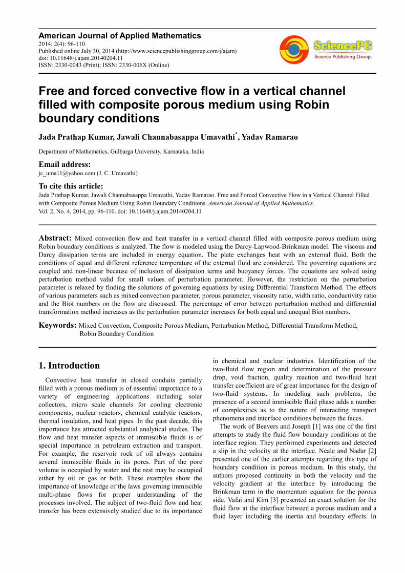
The geometry under consideration illustrated in figure. 1
consists of two infinite parallel plates maintained at equal
or different constant temperatures extending in the X and
Z directions. The region 1 2 0h Y− ≤ ≤ is occupied by a
fluid-saturated porous medium of permeability 1
κ , density
1ρ , viscosity
1µ , thermal conductivity
1k , and thermal
expansion coefficient 1
β , and the region 20 2Y h≤ ≤ is
occupied by another porous medium of permeability 2
κ ,
density 2
ρ , viscosity 2
µ , thermal conductivity 2
k , and
thermal expansion coefficient 2
β . The fluids are assumed
to have constant properties except the density in the
buoyancy term in the momentum equation
American Journal of Applied Mathematics 2014; 2(4): 96-110 98
( )1 0 1 1 01 T Tρ ρ β= − − and ( )2 0 2 2 01 T Tρ ρ β= − − . A fluid
rises in the channel driven by buoyancy forces. The
transport properties of both fluids are assumed to be
constant.
Fig 1: Physical configuration
We consider the fluids to be incompressible and the flow
is steady, laminar, and fully developed. It is assumed that
the only non-zero component of the velocity q�
are the X-
component ( 1,2)i
U i = . Thus, as a consequence of the mass
balance equation, one obtains
0iU
X
∂=
∂ (1)
so that iU depends only on Y . The stream wise and the
transverse momentum balance equations yields
( )2
1 11 1 0 1 12
1 1
10
d UPg T T U
X dY
νβ νρ κ
∂− − + − =∂
(2)
Region-II
( )2
2 22 2 0 2 22
2 2
10
d UPg T T U
X dY
νβ νρ κ
∂− − + − =∂
(3)
and Y -momentum balance equation in both the regions
can be expressed as
0P
Y
∂ =∂
(4)
where 0P p gxρ= + (assuming 1 2p p p= = ) is the
difference between the pressure and hydrostatic pressure.
On account of (4) P depends only on X so that (2) and (3)
can be rewritten as
Region-I
2
1 1 11 0 12
1 1 1 1 1
1 d UdPT T U
g dX g gdY
ν νβ ρ β β κ
− = − + (5)
Region-II
2
2 2 22 0 22
2 2 2 2 2
1 d UdPT T U
g dX g gdY
ν νβ ρ β β κ
− = − + (6)
From (5) and (6) one obtains
Region-I
2
1
2
1 1
1T d P
X g dXβ ρ∂
=∂
(7)
3
1 1 1 1 1
3
1 1 1
T d U dU
Y g g dYdY
ν νβ β κ
∂= − +
∂ (8)
2 4 2
1 1 1 1 1
2 4 2
1 1 1
T d U d U
g gY dY dY
ν νβ β κ
∂= − +
∂ (9)
Region-II
2
2
2
2 2
1T d P
X g dXβ ρ∂
=∂
(10)
3
2 2 2 2 2
3
2 2 2
T d U dU
Y g g dYdY
ν νβ β κ
∂= − +
∂ (11)
2 4 2
2 2 2 2 2
2 4 2
2 2 2
T d U d U
g gY dY dY
ν νβ β κ
∂= − +
∂ (12)
Both the walls of the channel will be assumed to have a
negligible thickness and to exchange heat by convection
with an external fluid. In particular, at 1 2Y h= − the
external convection coefficient will be considered as
uniform with the value 1q and the fluid in the region
1 2 0h Y− ≤ ≤ will be assumed to have a uniform reference
temperature1qT . At 2 2Y h= the external convection
coefficient will be considered as uniform with the value
2q and the fluid in the region 20 2Y h≤ ≤ will be
supposed to have a uniform reference temperature2 1q qT T≥ .
Therefore, the boundary conditions on the temperature field
can be expressed as
( )( )1
1
1
1 1 1 1
2
, 2q
hY
Tk q T T X h
Y =−
∂− = − −
∂ (13)
( )( )2
2
2
2 2 2 2
2
, 2q
hY
Tk q T X h T
Y =
∂− = −
∂ (14)
On account of (8) and (11), (13) and (14) can be
rewritten as
( )( )1
3
1 1 1
1 1 13
1 1 1
1, 2q
d U dU gq T T X h
dY kdY
βκ ν
− = − − at 1
2
hY = − (15)

99 Jada Prathap Kumar et al.: Free and Forced Convective Flow in a Vertical Channel Filled with Composite Porous
Medium Using Robin Boundary Conditions
( )( )2
3
2 2 22 2 23
2 2 2
1, 2 q
d U dU gq T X h T
dY kdY
βκ ν
− = − at 2
2
hY = (16)
On account of (5) and (6), there exist a constant A such
that
dPA
dX= (17)
For the problem under examination, the energy balance
equation in the presence of viscous dissipation can be
written as
Region-I
22
21 1 1 1
12
1 1 1p p
d T dUU
C dY CY
ν να κ α
= − − ∂ (18)
Region-II
22
22 2 2 2
22
2 2 2p p
d T dUU
C dY CY
ν να κ α
= − − ∂ (19)
From (9), (18), (12) and (19) allow one to obtain
differential equations for iU namely
Region-I
24 2 21 1 1 1
14 21 1 1 1 1
1 1
p p
d U d U dU Ug
g c dY cdY dYβ
β κ α κ α
= + +
(20)
Region-II
24 2 22 2 2 2
24 22 2 2 2 2
1 1
p p
d U d U dU Ug
g c dY cdY dYβ
β κ α κ α
= + +
(21)
The boundary conditions on velocity are no-slip
conditions, and those induced by boundary conditions on
temperature. In addition, the continuity of velocity, shear
stress, temperature and heat flux at the interface between
the two porous layers are assumed as:
( ) ( )1 1 2 22 2 0U h U h− = = (22)
together with (15) and (16) which on account of (5) and
(6) can be rewritten as
( )1
3 2
1 1 1 1 1 1 1
03 2
1 1 1 1 1 1
1q
d U dU q d U q g q AT T
dY k k kdY dY
βκ ν µ
− − = − − at
1
2
hY = −
( )2
3 2
2 2 2 2 2 2 2
03 2
2 2 2 2 2 2
1q
d U dU q d U q q gAT T
dY k k kdY dY
βκ µ ν
− + = − − at
2
2
hY = (23)
( ) ( )1 20 0U U= ,
( ) ( )1 2
1 2
0 0dU dU
dY dYµ µ= , ( ) ( )1 2
0 0T T= ,
( ) ( )1 2
1 2
0 0dT dTk k
dY dY= (24)
Equations (20)-(24) determine the velocity distribution.
They can be written in a dimensionless form by means of
the following dimensionless parameters
( )1
1 1
0
Uu
U= , ( )
2
2 2
0
Uu
U= , 1
1
1
Yy
D= , 2
2
2
Yy
D= ,
3
1 1
2
1
g TDGr
βν∆
= ,
( )1
0 1
1
ReU D
ν= ,
( )21
0 1
1
UBr
k T
µ=
∆ ,
Re
GrΛ = , 1 0
1
T T
Tθ −
=∆
,
2 0
2
T T
Tθ −
=∆
, 2 1T
T TR
T
−=
∆, 1
1 21
DaD
κ= , 2
2 22
DaD
κ= ,
1 1
1
1
h DBi
k= , 2 2
2
2
h DBi
k= , 1 2
1 2 1 22 2
Bi Bis
Bi Bi Bi Bi=
+ + (25)
The reference velocity and the reference temperature are
given by
( )2
1 1
0
148
ADU
µ= − ,
( )2
2 2
0
248
ADU
µ= − , ( )1 2
2 10
1 2
1 1
2
q q
q q
T TT s T T
Bi Bi
+ = + − −
(26)
Moreover, the temperature difference T∆ is given by
2 1q qT T T∆ = − if
1 2q qT T< . As a consequence, the
dimensionless parameter TR can only take the values 0 or 1.
More precisely, the temperature difference ratio TR is equal
to 1 for asymmetric heating i.e.1 2q q
T T< , while TR =0 for
symmetric heating i.e. 1 2q q
T T= , respectively. Equation (17)
implies that A can be either positive or negative. If 0A < ,
then 0
iU , Re , and Λ are negative, i.e. the flow is
downward. On the other hand, if 0A > , the flow is upward,
so that 0
iU , Re , and Λ are positive. Using (25) and (26),
(20)-(24) becomes
Region-I
24 2 2
1 1 1 1
4 2
1 1
1d u d u du uBr
Da dy Dady dy
− = Λ +
(27)
Region-II
24 2 242 2 2 2
4 2
2 2
1d u d u du uBr bh knm
Da dy Dady dy
− = Λ +
(28)
The boundary and interface conditions becomes
( ) ( )1 21 4 1 4 0u u− = = ,
American Journal of Applied Mathematics 2014; 2(4): 96-110 100
2 3
1 1 1
2 3
1 1 1 11 4
1 1 448 1
2
T
y
d u du d u R s
Da Bi dy Bi Bidy dy=−
Λ+ − = − + +
,
2 3
2 2 2
2 3
2 2 2 21 4
1 1 448 1
2
T
y
d u d u du R sbn
Bi Bi Da dy Bidy dy =
Λ+ − = − − +
,
( ) ( )2
1 20 0u mh u= , ( ) ( )1 20 0du du
hdy dy
= ,
2 2
1 1 2 2
2 2
1 2
1 148 1
d u u d u u
Da nb Da nbdy dy
− = − + −
at 0Y =
3 3
1 1 2 2
3 3
1 2
1 1 1d u du d u du
Da dy nbkh Da dydy dy
− = −
at 0Y = (29)
2.1. Basic Idea of Differential Transformation Method
(DTM)
If ( )u y is analytic in the time domain T, then it will be
differentiated continuously with respect to y in the domain
of interest. The differential transform of function ( )u y is
defined as
( )0
1( )
!
k
k
y
d u yU k
k dy=
=
(30)
where ( )u y is the original function and ( )U k is the
transformed function which is called the T-function.
The differential inverse transform of ( )U k is defined as
follows:
( ) ( )0
k
k
u y U k y∞
=
=∑ (31)
In real applications, the function ( )u y by a finite series
of (31) can be written as
( ) ( )0
nk
k
u y U k y=
=∑ (32)
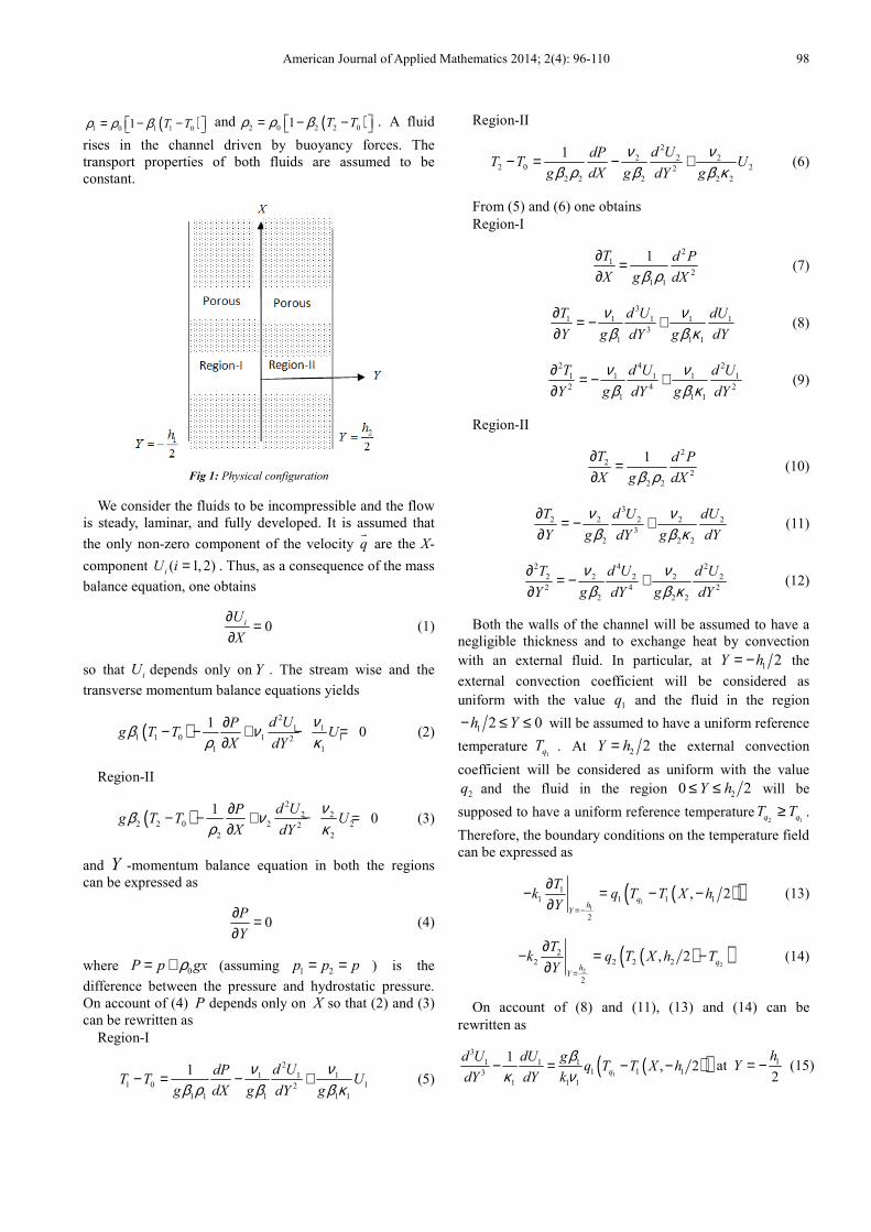
Table 1: The operations for the one-dimensional differential transform
method.
Original function Transformed function
( ) ( ) ( )y x g x h x= ± ( ) ( ) ( )Y k G k H k= ±
( ) ( )y x g xα= ( ) ( )Y k G kα=
( )( )
dg xy x
dx= ( ) ( 1) ( 1)Y k k G k= + +
2
2
( )( )
d g xy x
dx= ( ) ( 1)( 2) ( 2)Y k k k G k= + + +
( ) ( ) ( )y x g x h x= 0
( ) ( ) ( )k
l
Y k G l H k l=
= −∑
( ) my x x= 1, if
( ) ( )0, if
k mY k k m
k mδ
== − = ≠
and (31) implies that ( ) ( )1
k
k n
u y U k y∞
= +
= ∑ and is
neglected as it is small. Usually, the values of n are decided
by a convergence of the series coefficients. The
fundamental mathematical operations performed by
differential transform method are listed in Table 1.
3. Solutions
3.1. Special Cases
3.1.1. Case of Negligible Viscous Dissipation ( )0Br =
The solution of (27) and (28) using boundary and
interface conditions in (29) in the absence of viscous
dissipation term ( )0Br = is given by
Region-I
( ) ( )1 1 2 3 1 4 1cosh sinhu l l y l M y l M y= + + + (33)
Region-II
( ) ( )2 5 6 7 2 8 2cosh sinhu l l y l M y l M y= + + + (34)
where ( )1 11M Da= , ( )2 2
1M Da=
Using (29) in (5) and (6), the energy balance equations
becomes
Region-I
2
1 11 2
1
148
d u u
Dadyθ
= − − + Λ
(35)
Region-II
2
2 22 2
2
148
d u u
bn Dadyθ
= − − + Λ
(36)
Using the expressions obtained in (33) and (34) the
energy balance (35) and (36) becomes
Region-I
( ) ( ) ( )1 2
1 1 1 2 1
1
148 cosh sinh
l l yr M y r M y
Daθ
+ = − + + + Λ
(37)
Region-II
( ) ( ) ( )5 6
2 3 2 4 2
2
148 cosh sinh
l l yr M y r M y
bn Daθ
+ = − + + + Λ
(38)
3.1.2. Case of Negligible Buoyancy Force ( )0Λ =
The solution of (27) and (28) can be obtained when
buoyancy forces are negligible ( 0Λ = ) and viscous
dissipation is dominating ( 0Br ≠ ), so that purely forced
convection occurs. For this case, solutions of (27) and (28),
using the boundary and interface conditions given by (29),
the velocities are given by
Region-I
101 Jada Prathap Kumar et al.: Free and Forced Convective Flow in a Vertical Channel Filled with Composite Porous
Medium Using Robin Boundary Conditions
( ) ( )1 1 2 3 1 4 1cosh sinhu f f y f M y f M y= + + + (39)
Region-II
( ) ( )2 5 6 7 2 8 2cosh sinhu f f y f M y f M y= + + + (40)
The energy balance (18) and (19) in non-dimensional
form can also be written as
Region-I
22 2
1 1 1
2
1
d du uBr
dy Dady
θ = − +
(41)
Region-II
22 2
42 2 2
2
2
d du uBr k m h
dy Dady
θ = − +
(42)
The boundary and interface conditions for temperature
are
( )1 1
1 1
11 4
41 4 1
2
T
y
d Bi R sBi
dy Bi
θ θ=−
− − = +
,
( )2 2
2 2
21 4
41 4 1
2
T
y
d Bi R sBi
dy Bi
θ θ=
+ = +
,
( ) ( )1 20 0θ θ= ,
( ) ( )1 20 01d d
dy kh dy
θ θ= (43)
Using (39) and (40), solving (41) and (42) we obtain
Region-I
( )( ( ) ( ) ( )( ) ( ) )
1 10 1 11 1 12 1 13 1
4 3 2
14 1 15 1 16 17 18 1 2
cosh 2 sinh 2 cosh sinh
cosh sinh
Br p M y p M y p M y p M y
p y M y p y M y p y p y p y c y c
θ = − + + + +
+ + + + + + (44)
Region-II
( )( ( ) ( ) ( )( ) ( ) )
4
2 28 2 29 2 30 2 31 2
4 3 2
32 2 33 2 34 35 36 3 4
cosh 2 sinh 2 cosh sinh
cosh sinh
Br mkh p M y p M y p M y p M y
p y M y p y M y p y p y p y c y c
θ = − + + +
+ + + + + + + (45)
3.2. Perturbation Method (PM)
3.2.1. Combined Effects of Buoyancy Forces and Viscous
Dissipation
We solve (27) and (28) using the perturbation method
with a dimensionless parameter ε (<<1) defined as
Brε = Λ (46)
which does not depend on the reference temperature
difference T∆ . To this end the solutions are assumed in the
form
( ) ( ) ( ) ( ) ( )2
0 1 2
0
...n
n
n
u y u y u y u y u yε ε ε∞
=
= + + + =∑ (47)
Substituting (47) in (27) and (28) and equating the
coefficients of like powers of ε to zero, we obtain the zero
and first order equations as follows:
Region-I
Zero-order equations
4 2
10 10
4 2
1
10
d u d u
Dady dy− = (48)
First-order equations
2 24 2
10 1011 11
4 2
1 1
1 du ud u d u
Da dy Dady dy
− = +
(49)
Region-II
Zero-order equations
4 2
20 20
4 2
2
10
d u d u
Dady dy− = (50)
First-order equations
2 24 2
20 2021 2114 2
2 2
1 du ud u d uz
Da dy Dady dy
− = +
(51)
The corresponding boundary and interface conditions
given by (29) for the zeroth and first order reduces to
Zero-order
( ) ( )10 201 4 1 4 0u u− = =
, ( ) ( )2
10 200 0u mh u=,
( ) ( )10 200 0du du
hdy dy
= ,
2 2
10 10 20 20
2 2
1 2
1 148 1
d u u d u u
Da nb Da nbdy dy
− = − + −
at 0y = ,
3 3
10 10 20 20
3 3
1 2 2
1 1 1d u du d u du
Da dy z Da dydy dy
− = −
at 0y = ,
2 3
10 10 10
2 3
1 1 1 11 4
1 1 448 1
2
T
y
d u du d u R s
Da Bi dy Bi Bidy dy=−
Λ+ − = − + +
,
American Journal of Applied Mathematics 2014; 2(4): 96-110 102
2 3
20 20 20
2 3
2 2 2 21 4
1 1 448 1
2
T
y
d u d u du R sbn
Bi Bi Da dy Bidy dy=
Λ+ − = − − +
(52)
First-order
( ) ( )11 211 4 1 4 0u u− = =
, ( ) ( )2
11 210 0u mh u=,
( ) ( )11 210 0du du
hdy dy
=
2 2
11 11 21 21
2 2
1 2
1d u u d u u
Da nb Dady dy
− = −
at 0y = ,
3 3
11 11 21 21
3 3
1 2 2
1 1 1d u du d u du
Da dy z Da dydy dy
− = −
at 0y =
2 3
11 11 11
2 3
1 1 1 1 4
1 10
y
d u du d u
Da Bi dy Bidy dy =−
+ − =
,
2 3
21 21 21
2 3
2 2 2 1 4
1 10
y
d u d u du
Bi Da Bi dydy dy =
+ − =
(53)
Solutions of zeroth-order (48) and (50) using boundary
and interface conditions (52) are
( ) ( )10 1 2 3 1 4 1cosh sinhu H H y H M y H M y= + + +
(54)
( ) ( )20 5 6 7 2 8 2cosh sinhu H H y H M y H M y= + + + (55)
Solutions of first-order (49) and (51) using boundary and
interface conditions of (53) are
( ) ( ) ( )( ) ( ) ( ) ( )
( )
11 9 10 11 1 12 1 10 1
2
11 1 12 1 13 1 14 1
2 4 3 2
15 1 16 17 18
cosh sinh cosh 2
sinh 2 sinh cosh cosh
sinh
u H H y H M y H M y k M y
k M y k y M y k y M y k y M y
k y M y k y k y k y
= + + + + +
+ + + +
+ + + (56)
( ) ( ) ( )(( ) ( ) ( ) ( )
( ) )
21 13 14 15 2 16 2 1 28 2
2
29 2 30 2 31 2 32 2
2 4 3 2
33 2 34 35 36
cosh sinh cosh 2
sinh 2 sinh cosh cosh
sinh
u H H y H M y H M y t k M y
k M y k y M y k y M y k y M y
k y M y k y k y k y
= + + + + +
+ + + +
+ + +
(57)
Using velocities given by (54)-(57), the expressions for energy balance (35) and (36) becomes
Region-I
( ( )( ( ) ( )
( ) ( ) ( )( )( ) ( )( ) ( )
( ) ( )) ( ))
2 2
1 1 10 1 1 11 1 1 12 1
1 13 1 14 1 1 1
2 4 2 3 2 2
15 1 1 1 1 16 1 17 16 1 18
2 2 2
17 1 10 18 1 9 1 1 2
148 3 cosh 2 3 sinh 2 2 cosh
2 sinh 4 sinh 2cosh
4 cosh 2sinh 12
6 2
M k M y M k M y M k M y
M k M y k M y M y M y
k M y M y M y M k y M k y k M k y
k M H y k M H M H H y
θ ε= − − + +Λ+ + +
+ + + + + +
+ + + + + +
(58)
Region-II
( (( ( ) ( ) ( )
( ) ( ( ) ( )) ( )(( )) )( ) ( )
( )) ( ))
2 2
2 1 2 28 2 2 29 2 2 30 2
2 31 2 32 2 2 2 33 2 2
2 4 3 2 2
2 2 34 35 1 34 2 36 1 35 1 36
2 2
2 13 14 2 5 6
148 3 cosh 2 3 sinh 2 2 cosh
2 sinh 4 sinh 2cosh 4 cosh
2sinh 12 6 2
z M k M y M k M y M k M ybn
M k M y k M y M y M y k M y M y
M y M k y k y z k M k y z k y z k
M H H y M H H y
θ ε= − − + +Λ
+ + + +
+ + + + + + +
+ + + +
(59)
3.3. Solution with Differential Transform Method
Now Differential Transformation method has been applied for solving (27) and (28).Taking the differential
transformation of (27) and (28) with respect to k , and following the process as given in Table 1 yields:

103 Jada Prathap Kumar et al.: Free and Forced Convective Flow in a Vertical Channel Filled with Composite Porous
Medium Using Robin Boundary Conditions
( )( )( )( ) ( )( ) ( )
( )( )1
0 01
1 1( 4) 1 2 2
1 2 3 4
11 1 ( 1) ( 1) ( ) ( )
r r
s s
U r r r U rr r r r Da
Br r s s U r s U s U s U r sDa= =
+ = + + ++ + + +
+ Λ − + + − + + + −
∑ ∑ (60)
( )( ) ( )( )( )( ) ( )
2
4
0 02
1 ( 1)( 2)( 4) ( 2)
1 2 3 4
11 1 ( 1) ( 1) ( )
r r
s s
r rV r V r
r r r r Da
Br b n k m h r s s V r s V s V r s V sDa= =
+ ++ = ++ + + + + Λ − + + − + + + −
∑ ∑
(61)
The differential transform of the initial conditions are as follows
( ) ( ) ( ) ( )3 4
1 20 , 1 , 2 , 3 ,
2 6
c cU c U c U U= = = = ( ) 1
20
cV
mh= , ( ) 21 ,
cV
h=
( ) ( ) ( )1 1
3 4 2 2 2 22
1 2
12 48 1 , 3
c cV nb c V c c Da nbkh c h Da
nb Da Da nbmh
= − − − + = − +
(62)
where ( )U r and ( )V r are the transformed versions of
( )1u y and ( )2
u y respectively.
Using the conditions as given in (62), one can evaluate
the unknowns 1c , 2c , 3c , and 4c . By using the DTM and
the transformed boundary conditions, above equations that
finally leads to the solution of a system of algebraic
equations.
A Nusselt number can be defined at each boundary, as
follows:
( )1
1 2 11
2 2 1 12
2( )
2 ( 2) (1 )T TY h
h h dTNu
dYR T h T h R T=−
+=
− − + − ∆
( )2
1 2 22
2 2 1 12
2( )
2 ( 2) (1 )T TY h
h h dTNu
dYR T h T h R T=
+=
− − + − ∆ (63)
By employing (26), in (64) can be written as
( )1
1
2 11 4
(1 )
1 4 ( 1 4) (1 )T Ty
dhNu
dyR R
θθ θ
=−
+=− − + −
( )2
2
2 11 4
(1 1 )
1 4 ( 1 4) (1 )T Ty
dhNu
dyR R
θθ θ
=
+=− − + −
. (64)
All the constants appeared in the above equations are not
presented due to want of space.
4. Results and Discussion
The governing (28) and (29) subject to the boundary
conditions (30) have been solved analytically by regular
perturbation method valid for small values of perturbation
parameter ε . However this condition is relaxed by finding
the solutions valid for all values of ε by Differential
Transform method which is a semi-analytical method. Both
the cases of asymmetric ( )1T
R = and symmetric ( )0T
R =
wall heating conditions are considered and the results are
shown graphically in Figs. 2-13 for equal and unequal Biot
numbers. When 0Br = for equal Biot numbers, there is a
flow reversal for 400Λ = at the left wall and for
400Λ = − at the right wall as seen in Fig. 2. Further Fig. 2
also display the result that as σ increases velocity
decreases in both the regions for all values of Λ . The non-
dimensional temperature field θ is evaluated for different
values of Brinkman number in the case of negligible
buoyancy force which corresponds to 0Λ = for equal and
unequal Biot numbers in Figs. 3a and 3b respectively. The
temperature field is linear in the absence of mixed
convection parameter Λ and viscous dissipation ( )0Br =
indicating that the heat transfer is purely by conduction for
both equal and unequal Biot numbers. The temperature
field increases with increase in Brinkman number for both
equal and unequal Biot numbers. However the nature of
profiles for equal and unequal Biot numbers is different at
the cold plate. One should realize that this nature is due to
the fact that when1 2
0.1, 10Bi Bi= = , one obtains
( ) ( )2 2T L T L− > (following Zanchini, [26]). The effect
of Λ and Br for two fluid model is the similar result
observed by Zanchini [26] and Barletta [37] using
asymmetric wall heating conditions for one fluid model. To
compare the present results for one fluid model the values
of ratios of viscosity, width and conductivity are fixed as 1.
American Journal of Applied Mathematics 2014; 2(4): 96-110 104
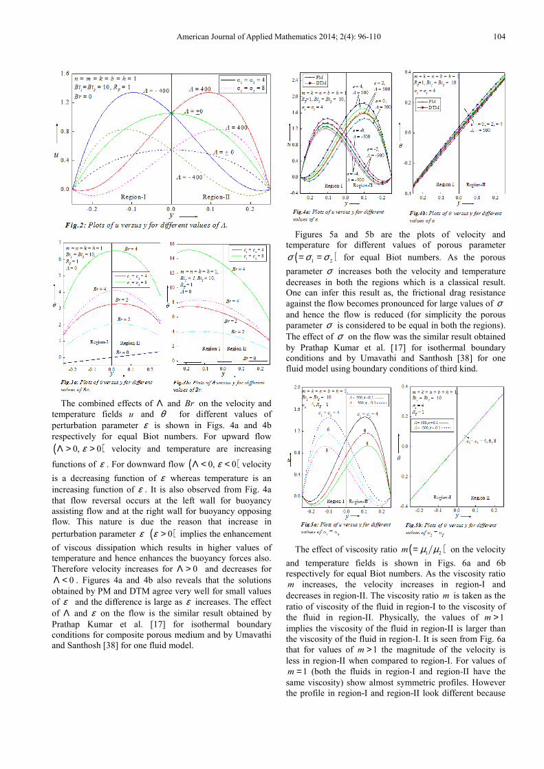
The combined effects of Λ and Br on the velocity and
temperature fields u and θ for different values of
perturbation parameter ε is shown in Figs. 4a and 4b
respectively for equal Biot numbers. For upward flow
( )0, 0εΛ > > velocity and temperature are increasing
functions of ε . For downward flow ( )0, 0εΛ < < velocity
is a decreasing function of ε whereas temperature is an
increasing function of ε . It is also observed from Fig. 4a
that flow reversal occurs at the left wall for buoyancy
assisting flow and at the right wall for buoyancy opposing
flow. This nature is due the reason that increase in
perturbation parameter ε ( )0ε > implies the enhancement
of viscous dissipation which results in higher values of
temperature and hence enhances the buoyancy forces also.
Therefore velocity increases for 0Λ > and decreases for
0Λ < . Figures 4a and 4b also reveals that the solutions
obtained by PM and DTM agree very well for small values
of ε and the difference is large as ε increases. The effect
of Λ and ε on the flow is the similar result obtained by
Prathap Kumar et al. [17] for isothermal boundary
conditions for composite porous medium and by Umavathi
and Santhosh [38] for one fluid model.
Figures 5a and 5b are the plots of velocity and
temperature for different values of porous parameter
( )1 2σ σ σ= = for equal Biot numbers. As the porous
parameter σ increases both the velocity and temperature
decreases in both the regions which is a classical result.
One can infer this result as, the frictional drag resistance
against the flow becomes pronounced for large values of σ
and hence the flow is reduced (for simplicity the porous
parameter σ is considered to be equal in both the regions).
The effect of σ on the flow was the similar result obtained
by Prathap Kumar et al. [17] for isothermal boundary
conditions and by Umavathi and Santhosh [38] for one
fluid model using boundary conditions of third kind.
The effect of viscosity ratio ( )1 2m µ µ= on the velocity
and temperature fields is shown in Figs. 6a and 6b
respectively for equal Biot numbers. As the viscosity ratio
m increases, the velocity increases in region-I and
decreases in region-II. The viscosity ratio m is taken as the
ratio of viscosity of the fluid in region-I to the viscosity of
the fluid in region-II. Physically, the values of 1m >
implies the viscosity of the fluid in region-II is larger than
the viscosity of the fluid in region-I. It is seen from Fig. 6a
that for values of 1m > the magnitude of the velocity is
less in region-II when compared to region-I. For values of
1m = (both the fluids in region-I and region-II have the
same viscosity) show almost symmetric profiles. However
the profile in region-I and region-II look different because

105 Jada Prathap Kumar et al.: Free and Forced Convective Flow in a Vertical Channel Filled with Composite Porous
Medium Using Robin Boundary Conditions
of the value of Λ chosen to be 500. Further there is a
continuity of velocity at the interface for 1m = and sudden
jump at the interface for values of 1m > . The fall at the
interface for values of 1m > is due to the nature of the
condition imposed at the interface. Figure 6b shows almost
no variation for the effects of m on the temperature. As the
porous parameter ( )1 2σ σ σ= = increases velocity
decreases in both regions. However the effect of σ is not
effective on the temperature field as seen in Fig. 6b.
The effect of width ratio ( )2 1h h h on the flow field is
shown in Figs. 7a and 7b respectively. The velocity and
temperature decreases in both regions as the width ratio h
increases. Physically, h increases imply width of the fluid
in region-I is wider than that of the fluid in region-II. The
magnitude of suppression is significant in region-I when
compared to region-II. Further from Fig. 7a one can also
explore that as ( )1 2σ σ σ= = increases velocity decreases
in both regions. Figure 7b also tells that the effect of σ is
not effective on the temperature field.
The velocity and temperature fields for variations of
conductivity ratio ( )1 2k k k are seen in Figs. 8a and 8b
respectively for equal Biot numbers. As k increases both
the velocity and temperature decreases in both regions.
Values of 1k > implies the thermal conductivity in region-
II is greater than the thermal conductivity in region-I.
Further as σ increases velocity decreases in both the
regions and is not effective on the temperature field.
The effect of Λ and ε for unequal Biot numbers on the
velocity and temperature field is displayed in Figs. 9a and
9b respectively. It is observed that for unequal Biot
numbers there is no flow reversal at both the cold and hot
walls for upward and downward flows when compared
with equal Biot numbers. Further the nature of temperature
profiles for unequal Biot numbers is more distinguishable
at the cold wall when compared with equal Biot numbers.
However the effect of Λ and ε for unequal Biot numbers
is similar to the equal Biot numbers. Comparing Figs. 4a, b
(equal Biot numbers) and Figs. 9a,b (unequal Biot numbers)
one can explore the result that the effect of Λ on u and θ
becomes stronger if either 1
Bi or 2
Bi becomes stronger.
The effect of porous parameter ( )1 2σ σ σ= = for
unequal Biot numbers on the flow field is depicted in Figs.
10a,b. The effect of σ on the flow for unequal Biot
numbers shows the similar nature as that on equal Biot
numbers (Fig. 5a, b). That is as σ increases velocity
decreases in both the regions for both buoyancy assisting
and buoyancy opposing flows. The effect of σ is not
changing the temperature field as seen Fig. 10b. The effect
of σ on the flow was the similar result obtained by
Umavathi and Santosh [38] for unequal Biot numbers for
one fluid model.
Figures 11a,b and 12a,b are the plots of u and θΛ for
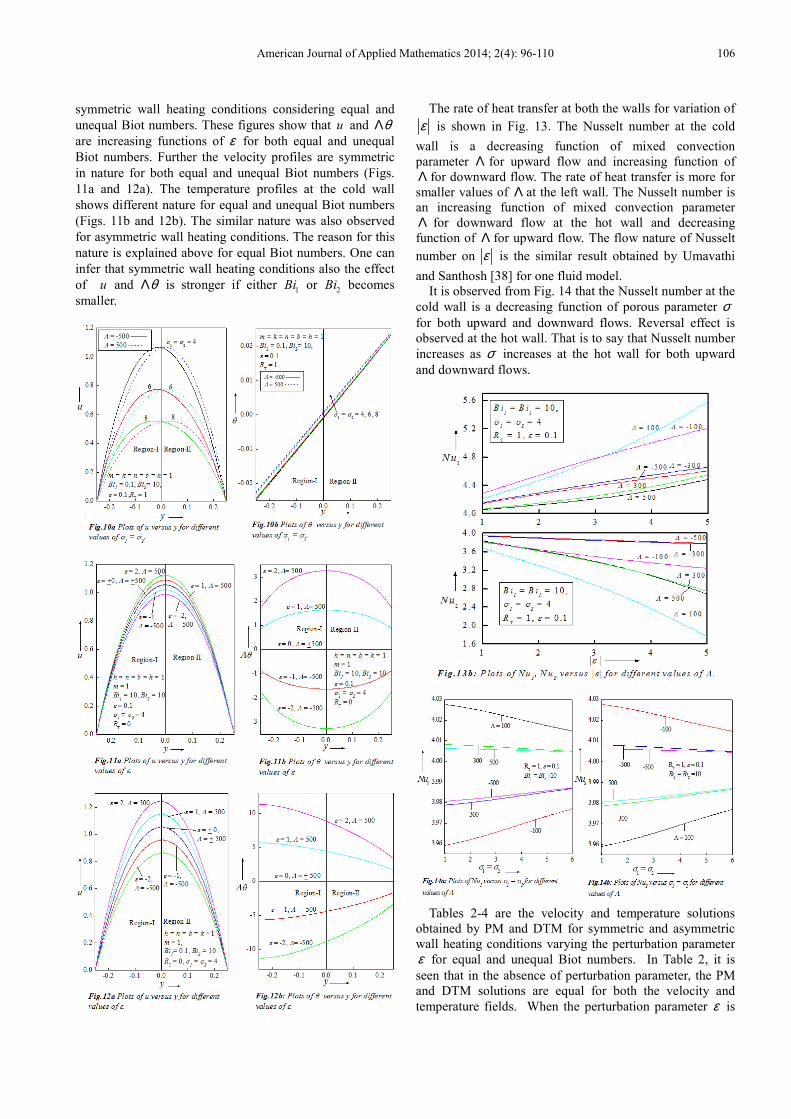
American Journal of Applied Mathematics 2014; 2(4): 96-110 106
symmetric wall heating conditions considering equal and
unequal Biot numbers. These figures show that u and θΛ
are increasing functions of ε for both equal and unequal
Biot numbers. Further the velocity profiles are symmetric
in nature for both equal and unequal Biot numbers (Figs.
11a and 12a). The temperature profiles at the cold wall
shows different nature for equal and unequal Biot numbers
(Figs. 11b and 12b). The similar nature was also observed
for asymmetric wall heating conditions. The reason for this
nature is explained above for equal Biot numbers. One can
infer that symmetric wall heating conditions also the effect
of u and θΛ is stronger if either 1
Bi or 2
Bi becomes
smaller.
The rate of heat transfer at both the walls for variation of
ε is shown in Fig. 13. The Nusselt number at the cold
wall is a decreasing function of mixed convection
parameter Λ for upward flow and increasing function of
Λ for downward flow. The rate of heat transfer is more for
smaller values of Λ at the left wall. The Nusselt number is
an increasing function of mixed convection parameter
Λ for downward flow at the hot wall and decreasing
function of Λ for upward flow. The flow nature of Nusselt
number on ε is the similar result obtained by Umavathi
and Santhosh [38] for one fluid model.
It is observed from Fig. 14 that the Nusselt number at the
cold wall is a decreasing function of porous parameter σ
for both upward and downward flows. Reversal effect is
observed at the hot wall. That is to say that Nusselt number
increases as σ increases at the hot wall for both upward
and downward flows.
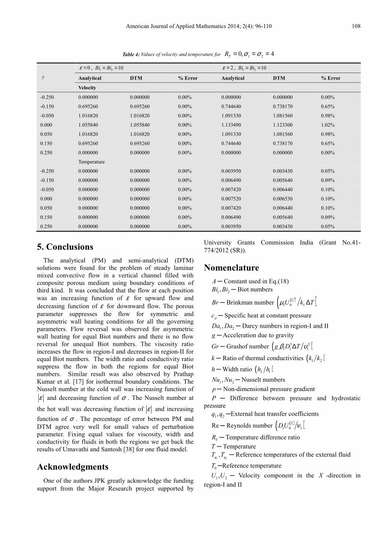
Tables 2-4 are the velocity and temperature solutions
obtained by PM and DTM for symmetric and asymmetric
wall heating conditions varying the perturbation parameter
ε for equal and unequal Biot numbers. In Table 2, it is
seen that in the absence of perturbation parameter, the PM
and DTM solutions are equal for both the velocity and
temperature fields. When the perturbation parameter ε is
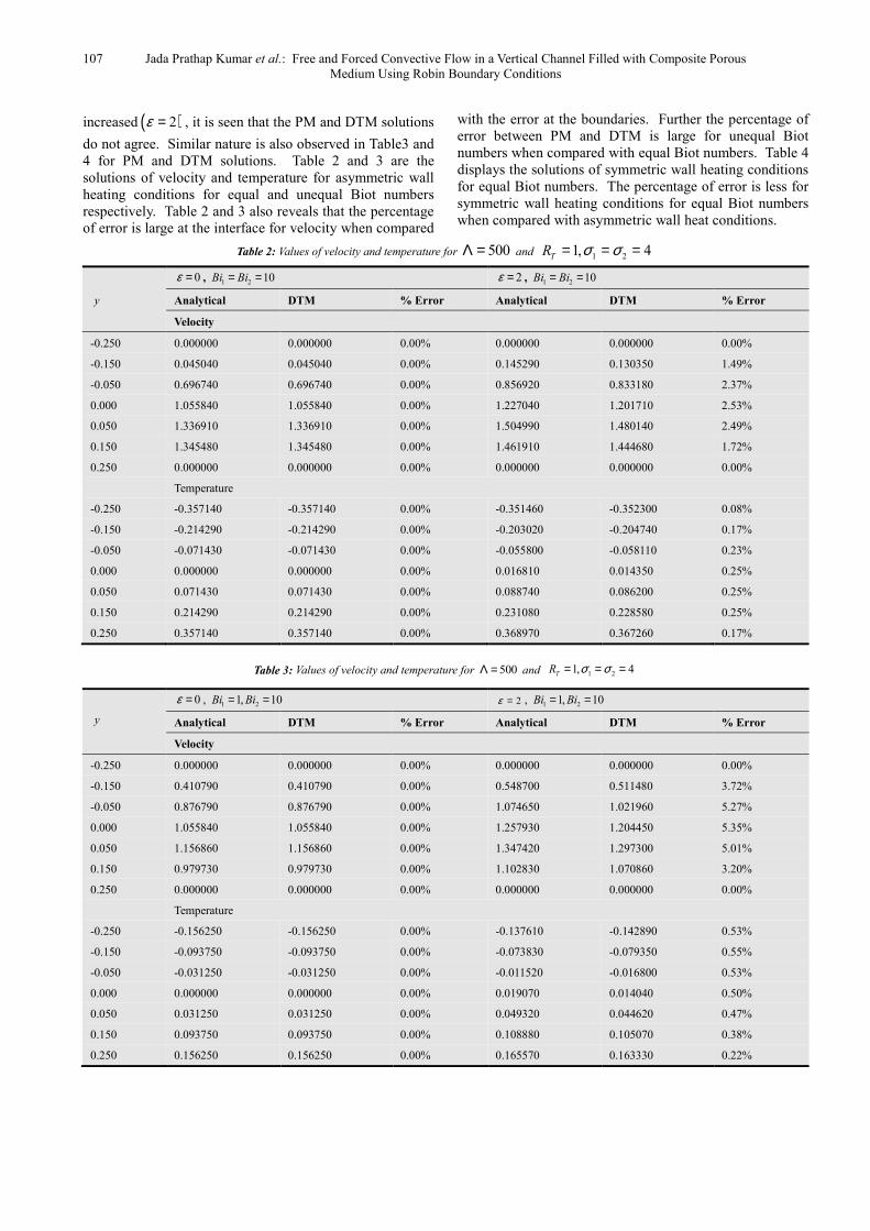
107 Jada Prathap Kumar et al.: Free and Forced Convective Flow in a Vertical Channel Filled with Composite Porous
Medium Using Robin Boundary Conditions
increased ( )2ε = , it is seen that the PM and DTM solutions
do not agree. Similar nature is also observed in Table3 and
4 for PM and DTM solutions. Table 2 and 3 are the
solutions of velocity and temperature for asymmetric wall
heating conditions for equal and unequal Biot numbers
respectively. Table 2 and 3 also reveals that the percentage
of error is large at the interface for velocity when compared
with the error at the boundaries. Further the percentage of
error between PM and DTM is large for unequal Biot
numbers when compared with equal Biot numbers. Table 4
displays the solutions of symmetric wall heating conditions
for equal Biot numbers. The percentage of error is less for
symmetric wall heating conditions for equal Biot numbers
when compared with asymmetric wall heat conditions.
Table 2: Values of velocity and temperature for 500Λ = and 1 21, 4TR σ σ= = =
y
0ε = , 1 2 10Bi Bi= = 2ε = , 1 2 10Bi Bi= =
Analytical DTM % Error Analytical DTM % Error
Velocity
-0.250 0.000000 0.000000 0.00% 0.000000 0.000000 0.00%
-0.150 0.045040 0.045040 0.00% 0.145290 0.130350 1.49%
-0.050 0.696740 0.696740 0.00% 0.856920 0.833180 2.37%
0.000 1.055840 1.055840 0.00% 1.227040 1.201710 2.53%
0.050 1.336910 1.336910 0.00% 1.504990 1.480140 2.49%
0.150 1.345480 1.345480 0.00% 1.461910 1.444680 1.72%
0.250 0.000000 0.000000 0.00% 0.000000 0.000000 0.00%
Temperature
-0.250 -0.357140 -0.357140 0.00% -0.351460 -0.352300 0.08%
-0.150 -0.214290 -0.214290 0.00% -0.203020 -0.204740 0.17%
-0.050 -0.071430 -0.071430 0.00% -0.055800 -0.058110 0.23%
0.000 0.000000 0.000000 0.00% 0.016810 0.014350 0.25%
0.050 0.071430 0.071430 0.00% 0.088740 0.086200 0.25%
0.150 0.214290 0.214290 0.00% 0.231080 0.228580 0.25%
0.250 0.357140 0.357140 0.00% 0.368970 0.367260 0.17%
Table 3: Values of velocity and temperature for 500Λ = and 1 21, 4TR σ σ= = =
y
0ε = , 1 21, 10Bi Bi= = 2ε = , 1 21, 10Bi Bi= =
Analytical DTM % Error Analytical DTM % Error
Velocity
-0.250 0.000000 0.000000 0.00% 0.000000 0.000000 0.00%
-0.150 0.410790 0.410790 0.00% 0.548700 0.511480 3.72%
-0.050 0.876790 0.876790 0.00% 1.074650 1.021960 5.27%
0.000 1.055840 1.055840 0.00% 1.257930 1.204450 5.35%
0.050 1.156860 1.156860 0.00% 1.347420 1.297300 5.01%
0.150 0.979730 0.979730 0.00% 1.102830 1.070860 3.20%
0.250 0.000000 0.000000 0.00% 0.000000 0.000000 0.00%
Temperature
-0.250 -0.156250 -0.156250 0.00% -0.137610 -0.142890 0.53%
-0.150 -0.093750 -0.093750 0.00% -0.073830 -0.079350 0.55%
-0.050 -0.031250 -0.031250 0.00% -0.011520 -0.016800 0.53%
0.000 0.000000 0.000000 0.00% 0.019070 0.014040 0.50%
0.050 0.031250 0.031250 0.00% 0.049320 0.044620 0.47%
0.150 0.093750 0.093750 0.00% 0.108880 0.105070 0.38%
0.250 0.156250 0.156250 0.00% 0.165570 0.163330 0.22%
American Journal of Applied Mathematics 2014; 2(4): 96-110 108
Table 4: Values of velocity and temperature for 1 20, 4TR σ σ= = =
y
0ε = , 1 2 10Bi Bi= = 2ε = , 1 2 10Bi Bi= =
Analytical DTM % Error Analytical DTM % Error
Velocity
-0.250 0.000000 0.000000 0.00% 0.000000 0.000000 0.00%
-0.150 0.695260 0.695260 0.00% 0.744640 0.738170 0.65%
-0.050 1.016820 1.016820 0.00% 1.091330 1.081560 0.98%
0.000 1.055840 1.055840 0.00% 1.133490 1.123300 1.02%
0.050 1.016820 1.016820 0.00% 1.091330 1.081560 0.98%
0.150 0.695260 0.695260 0.00% 0.744640 0.738170 0.65%
0.250 0.000000 0.000000 0.00% 0.000000 0.000000 0.00%
Temperature
-0.250 0.000000 0.000000 0.00% 0.003950 0.003430 0.05%
-0.150 0.000000 0.000000 0.00% 0.006490 0.005640 0.09%
-0.050 0.000000 0.000000 0.00% 0.007420 0.006440 0.10%
0.000 0.000000 0.000000 0.00% 0.007520 0.006530 0.10%
0.050 0.000000 0.000000 0.00% 0.007420 0.006440 0.10%
0.150 0.000000 0.000000 0.00% 0.006490 0.005640 0.09%
0.250 0.000000 0.000000 0.00% 0.003950 0.003430 0.05%
5. Conclusions
The analytical (PM) and semi-analytical (DTM)
solutions were found for the problem of steady laminar
mixed convective flow in a vertical channel filled with
composite porous medium using boundary conditions of
third kind. It was concluded that the flow at each position
was an increasing function of ε for upward flow and
decreasing function of ε for downward flow. The porous
parameter suppresses the flow for symmetric and
asymmetric wall heating conditions for all the governing
parameters. Flow reversal was observed for asymmetric
wall heating for equal Biot numbers and there is no flow
reversal for unequal Biot numbers. The viscosity ratio
increases the flow in region-I and decreases in region-II for
equal Biot numbers. The width ratio and conductivity ratio
suppress the flow in both the regions for equal Biot
numbers. Similar result was also observed by Prathap
Kumar et al. [17] for isothermal boundary conditions. The
Nusselt number at the cold wall was increasing function of
ε and decreasing function of σ . The Nusselt number at
the hot wall was decreasing function of ε and increasing
function of σ . The percentage of error between PM and
DTM agree very well for small values of perturbation
parameter. Fixing equal values for viscosity, width and
conductivity for fluids in both the regions we get back the
results of Umavathi and Santosh [38] for one fluid model.
Acknowledgments
One of the authors JPK greatly acknowledge the funding
support from the Major Research project supported by
University Grants Commission India (Grant No.41-
774/2012 (SR)).
Nomenclature
A ─ Constant used in Eq.(18)
1 2,Bi Bi ─ Biot numbers
Br ─ Brinkman number ( )( )21
1 0 1U k Tµ ∆
pc ─ Specific heat at constant pressure
1 2,Da Da ─ Darcy numbers in region-I and II
g ─ Acceleration due to gravity
Gr ─ Grashof number ( )3 2
1 1 1g D Tβ υ∆
k ─ Ratio of thermal conductivities ( )1 2k k
h ─ Width ratio ( )2 1h h
1 2,Nu Nu ─ Nusselt numbers
p ─ Non-dimensional pressure gradient
P ─ Difference between pressure and hydrostatic
pressure
1 2,q q ─External heat transfer coefficients
Re ─ Reynolds number ( )( )1
1 0 1DU ν
TR ─ Temperature difference ratio
T ─ Temperature
1 2,q qT T ─ Reference temperatures of the external fluid
0T ─Reference temperature
1 2,U U ─ Velocity component in the X -direction in
region-I and II

109 Jada Prathap Kumar et al.: Free and Forced Convective Flow in a Vertical Channel Filled with Composite Porous
Medium Using Robin Boundary Conditions
( )0
iU ─Reference velocity
1, 2u u ─ Dimensionless velocity in the X -direction in
region-I and II
X ─Stream wise coordinate
x ─Dimensionless stream wise coordinate
Y ─Transverse coordinate
y ─Dimensionless transverse coordinate
Greek Symbols
1α ,
2α ─Thermal diffusivity in region-I and II
1β ,
2β ─Thermal expansion coefficient in region-I and II
1 2,κ κ ─Permeability of porous medium in region-I and II
T∆ ─ Reference temperature difference ( )2 1q qT T−
ε ─ Dimensionless parameter
1 2,θ θ ─ Dimensionaless temperatures in region-I and II
1 2,µ µ ─Viscosity in region-I and II
1 2,ν ν ─ Kinematics viscosities in region-I and II
1 2,ρ ρ ─ Density of fluids in region-I and II
Λ ─Dimensionless parameter ( )ReGr
Subscripts
1 and 2 reference quantities for Region-I and II,
respectively
References
[1] G. Beavers, and D.D. Joseph, “Boundary conditions at a naturally permeable wall,” J. Fluid Mech, vol. 30: pp. 197-207, 1967.
[2] G. Neale, and W. Nadar, “Practical significance of Brinkman’s extension of Darcy’s law: Coupled parallel flows within a channel and a bounding porous medium,” Can. J. Chem. Engrg, vol. 52, pp. 475- 478, 1974.
[3] K. Vafai, and S.J. Kim, “Fluid mechanics of the inter-phase region between a porous medium and a fluid layer-an exact solution,” Int. J. Heat Fluid Flow, vol. 11, pp.254-256, 1990.
[4] K. Vafai, and R. Thiyagaraja, “Analysis of flow and heat transfer at the interface region of a porous medium,” Int. J. Heat Fluid Flow, vol. 30, pp. 1391-1405, 1987.
[5] K. Vafai, and S.J. Kim, “Analysis of surface enhancement by a porous substrate,” J. Heat Transfer, vol. 112, pp. 700-706, 1990.
[6] S.J. Kim, and C.Y. Choi, “Convection heat transfer in porous and overlaying layers heated from below,” Int. J. Heat Mass Transfer, vol. 39, pp. 319-329, 1996.
[7] D. Poulikakos, and M. Kazmierczak, “Forced convection in a duct partially filled with a porous material,” J. Heat Transfer, vol. 109, pp.653-662, 1987.
[8] J.A. Ochoa-Tapie, and S. Whitaker, “Heat transfer at the boundary between a porous medium and a homogeneous
fluid,” Int. J. Heat Mass Transfer, vol. 40, pp. 2691-2707, 1997.
[9] J.W. Paek, B.H. Kang, S.Y. Kim, and J.M. Hyan, “Effective thermal conductivity and permeability of aluminum foam materials,” Int. J. Thermophys, vol. 21, pp. 453-464, 2000.
[10] A.V. Kuznetsov, “Analytical study of fluid flow and heat transfer during forced convection in a composite channel partly filled with a Brinkman-Forchheimer porous medium,” Flow Turbulence and Combustion, vol. 60, pp. 173-192, 1998.
[11] D.A. Nield, and A.V. Kuznetsov, “The effect of heterogeneity in forced convection in a porous medium: parallel plate channel or circular duct,” Int. J. Heat Mass Transfer, vol. 43, pp. 4119-4134, 2000.
[12] M.S. Malashetty, J.C. Umavathi, and J. Prathap Kumar, “Convective Flow and Heat Transfer in an Inclined Composite Porous Medium,” J. Porous Media, vol. 4(1), pp. 15-22, 2001.
[13] M.S. Malashetty, J.C. Umavathi, and J. Prathap Kumar, “Two fluid flow and heat transfer in an inclined channel containing porous and fluid layer,” Heat and Mass Transfer, vol. 40, pp. 871–876, 2004.
[14] J.C. Umavathi, Ali J Chamkha, Abdul Mateen, and Al-Mudhaf A, “Oscillatory flow and heat transfer in a horizontal composite porous medium channel,” Int. J. Heat and Tech, vol. 25(2), pp. 75-86, 2006.
[15] J.C. Umavathi, M.S. Malashetty, and J. Prathap Kumar, “Flow and heat transfer in an inclined channel containing a porous layer sandwiched between two fluid layers,” ASME, Modelling Measurement and Controlling, vol. 74, pp. 19-35, 2005.
[16] J.C. Umavathi, J. Prathap Kumar, and K.S.R. Sridhar, “Flow and heat transfer of poiseuille.couette flow in an inclined channel for composite porous medium,” Int. J. Appl. Mech. Engg, vol. 15(1), pp. 249-266, 2010.
[17] J. Prathap Kumar, J.C. Umavathi, and Basavaraj M Biradar, “Mixed convection of composite potous medium in a vertical channel with asymmetrical wall heating conditions,” J. Porous Media, vol. 13(3), pp. 271-285, 2010.
[18] J. Prathap Kumar, J.C. Umavathi, I. Pop, and Basavaraj M Biradar, “Fully developed mixed convection flow in a vertical channel containing porous and fluid layer with isothermal or isoflux boundaries,” Trans. Porous Med, vol. 80, pp. 117–135, 2009.
[19] P. Wibulswas, “Laminar flow heat transfer in non circular ducts,” Ph.D. Thesis, London University, 1966 (as reported by Shah and London in 1971)
[20] R.W. Lyczkowski, C.W. Solbrig, and D. Gidaspow, Forced convective heat transfer in rectangular ducts general case of wall resistance and peripheral conduction. 969. Institute of Gas Technology Tech. Info, Center File 3229, 3424S, State, Street, Chicago, Ill 60616 (as reported by Shah and London in 1971).
[21] V. Javeri, “Analysis of laminar thermal entrance region of elliptical and rectangular channels with Kantorowich method,” Warme- und Stoffuberragung, vol. 9, pp. 85–98, 1976.
American Journal of Applied Mathematics 2014; 2(4): 96-110 110
[22] E. Hicken, and Das, Temperatur field in laminar durchstromten Kanalen mitechteckquerschnitt bei unterschiedlicher Beheizung der Kanalwade,” Warme- und Stoffubertragung, vol. 1, pp. 98–104, 1968.
[23] E.M. Sparrow, R. Siegal, “Application of variational methods to the thermal entrance region of ducts,” Int. J. Heat Mass Transfer, vol. 1, pp. 161–172, 1960.
[24] V. Javeri, Heat transfer in laminar entrance region of a flat channel for the temperature boundary condition of the third kind,” Warne-und Stoffubertragung Thermo-and Fluid Dynamics, vol. 10, pp. 137-144, 1977.
[25] V. Javeri, “Laminar heat transfer in a rectangular channel for the temperature boundary conditions of third kind,” Int. J, Heat Mass Transfer, vol. 10, pp. 1029-1034, 1978.
[26] E. Zanchini, Effect of viscous dissipation on mixed convection in a vertical channel with boundary conditions of the third kind,” Int. J Heat and Mass Transfer, vol. 41, pp. 3949 –3959, 1998.
[27] M. Kumari, and G. Nath, “Mixed convection boundary layer flow over a thin vertical cylinder with localized injection/suction and cooling/heating,” Int. Heat mass Transfer, vol. 47, pp. 969-976, 2004.
[28] J.K. Zhou, “Differential transformation and its applications for electrical circuits,” Huarjung University Press, 1986. (in Chinese)
[29] M.J. Jang, C.L. Chen, and Y.C. Liu, “Two-dimensional differential transform for partial differential equations,” Appl. Math. Comput, vol 21, pp. 261–270, 2001.
[30] A. Kurnaz, and G. Oturanç, “The differential transform approximation for the system of ordinary differential equations,” Int. J. Comput. Math, vol. 82, pp. 709–719, 2005.
[31] A. Arikoglu, and I. Ozkol, “Solution of differential-difference equations by using differential transform method,” Appl. Math. Comput, vol. 181, pp. 153–62, 2006.
[32] A.S.V. Ravi Kanth, and K. Aruna, “Solution of singular two-point boundary value problems using differential transformation method,” Physics Letters A, vol. 372, pp. 4671–4673, 2008.
[33] M.J. Jang, Y.L. Yeh, C.L. Chen, and W.C. Yeh, “Differential transformation approach to thermal conductive problems with discontinuous boundary condition,” Appl., Math. Comput, vol. 216, pp. 2339–2350, 2010.
[34] M.M. Rashidi, N. Laraqi, and S. M. Sadri, “A novel analytical solution of mixed convection about an inclined flat plate embedded in a porous medium using the DTM-Padé,” Int. J. Thermal Sci, vol. 49, pp. 2405–2412, 2010.
[35] H. Yaghoobi, and M. Torabi, “The application of differential transformation method to nonlinear equations arising in heat transfer,” Int. Commu. Heat and Mass Transfer, vol. 38, pp. 815–820, 2011.
[36] M.M. Rashidi, O. Anwar Beg, and N. Rahimzadeh, “A generalized differential transform method for combined free and forced convection flow about inclined surfaces in porous media,” Chem. Eng. Comm, vol. 199, pp. 257–282, 2012.
[37] A. Barletta, “Laminar mixed convection with viscous dissipation in a vertical channel,” Int. J. Heat Mass Transfm, vol. 41, pp. 3501-3513, 1998.
[38] J.C. Umavathi, and V. Santosh, “Non-Darcy mixed convection in a vertical porous channel with boundary conditions of third kind,” Trans. Porous Media, vol. 95, pp. 111-131, 2012.


![Application of Partial Differential Equations to Drum Head ...article.sciencepublishinggroup.com/pdf/10.11648.j.ajam...Similarly [5] provided an algorithm of Elzaki projected differential](https://img.pdfslide.us/doc/110x75/5afbfbd97f8b9a434e8b8649/application-of-partial-differential-equations-to-drum-head-5-provided-an-algorithm.jpg)