Embed Size (px)
Citation preview

POLITECNICO DI MILANO
Energy Department
Numerical Simulation of non-Reactive Evaporative Diesel
Sprays Using OpenFoam
Supervisor
Prof. Tommaso Lucchini
Master’s Degree Thesis of
Alireza Ghasaemi, matr. 816931
Academic Year 2016/2017

What follows is a 15 page summary of this work. The reader is encouraged to refer to the full report for better clarifications and further reading on the details.

1
Numerical Simulation of non-Reactive Evaporative Diesel Sprays Using OpenFoam
Summary of Master’s Degree Thesis of Alireza Ghasemi, matr. 816931 Politecnico di Milano, 2017
Supervisor: Prof. Tommaso Lucchini
Abstract
Computational methods have been an indispensable tool in rapid engine design and improvement. Difficulties in direct experimental measurements of the optically thick liquid core in the diesel fuel injection, which occurs at high temporal and spatial resolutions, has resulted in various breakup models and method to describe the injection physics.
This work focuses on Eulerian-Lagrangian CFD simulation of the fuel injection inside the diesel combustion chamber in non-reactive conditions using Lib-ICE, an OpenFOAM Library. The model was tuned so that the simulation results were in agreement with the results of experimental data with regards to parameters such as liquid and vapor penetration and the spray mixing line. The case tuning involved turbulence model coefficient adjustment, turbulent Schmidt number modification and adjusting the parameters regarding a blob-KH/RT breakup scheme. Simulation fidelity with respect to ambient gas temperatures as well as simulating various spray nozzles was examined and discussed. The results was presented as contribution to the fifth ECN workshop under the third topic regarding evaporative spray simulation.
Keywords: CFD, OpenFOAM, Lib-ICE, Diesel, non-Reactive Spray, Breakup, KH/RT, ECN, Mixing Line
Introduction
Liquid spray simulation concerns a wide range of natural phenomenon present in a variety of technical systems and industrial applications. One of the main area of focus for this type of fluid simulation is the diesel sprays. Due to their reliability, better part load operation, fuel flexibility, etc. diesel engines have been widely adopted from medium-low to high power units [1, 2].
From an environmental perspective, the growing concerns on human caused global climate change [3] as well as the adverse health effects of exposure to gaseous and particulate components of vehicular emissions [4, 5] have been historically pushing the industry to lower the diesel engine emissions. Furthermore, the global energy demands have been calling for better fuel economy in modern engines and thus, the diesel engine has been undergoing a rapid development and refinement ever since its commercialization with the two main objectives of lowering engine emission levels, and preserving performance and improving fuel economy [6, 7]. Nevertheless, the relentless development of diesel
engines in the last decades has been largely a consequence of the improvement of the injection systems performance and flexibility and the implementation of new combustion strategies [8].
The modern methods of fluid simulation have been a key factor in these rapid improvements over the years and have proved beneficial as opposed to conventional methods of prototyping since numerical simulation can be used to investigate processes that take place at time and length scales or in places that are not accessible and thus cannot be easily investigated using experimental techniques [2, 9]. This is crucial since there are many challenges associated with measuring diesel injection since spray breakup is characterized in the orders of micrometers and nanoseconds and the optically thick nature of the liquid core near the nozzle could introduce significant uncertainty in optical measurements [10]. By utilizing computational fluid dynamics (CFD) in conjunction with experiments in has been possible to drastically reduce the time and cost associated with diesel engine development [11].
This project was defined around the participation of Politecnico di Milano in the fifth edition of the Engine

2
Combustion Network (ECN) workshop [12], on the topic of diesel spray mixing and evaporation. More specifically, it involved computational fluid dynamic simulation of the fuel injection inside the diesel combustion chamber in non-reactive conditions with a focus on three specific injectors dubbed Spray A,C and D. The non-reactive injection is simulated with the aim of better understanding of the liquid core breakup and the subsequent formation of droplets and evaporation in the implemented method. The focus was on some of the most important parameters in diesel spray vaporization process i.e. the penetration length of liquid and vapor and the spray mixing line. The effects of various simulation parameters such as the breakup scheme coefficients and ambient temperature were studied.
An invaluable database of experimental tests conducted by various participating institutions in the ECN was utilized for simulation validation purposes and model tuning. The results were presented in the ECN5 conference held at Wayne State University in Detroit, USA, along with the contributions from other participating institutions and groups.
The ECN is an international collaboration among experimental and computational researchers in engine combustion. The aim is to establish an internet library of well-documented experiments that are appropriate for model validation and the advancement of scientific understanding of combustion at conditions specific to engines. In this work, a CFD solver for combustion simulation in direct injection Diesel engines has been implemented in Lib-ICE, an OpenFOAM library for internal combustion engine simulations developed by the ICE group of Politecnico di Milano.
Eulerian Phase
The gas medium is treated in an Eulerian fashion and the spray evolves into the domain based on the mass, momentum and energy exchange with the continuous gas phase. For the gas phase, the mass, momentum and energy equations are solved for a compressible, multi-component gas flow using the RANS approach. The equations are described in brief according to [11,
18]. Considering an infinitesimal flow element which is fixed in space, we can obtain the continuity equation in conservation form by applying the mass conservation principal:
𝜕𝜌𝜕𝑡
+ ∇. (𝜌.U) = 𝑆�̇� (1)
The conservation of species mass fraction:
𝜕𝜌𝑌𝑖𝜕𝑡
+ 𝛻. (𝜌.U𝑌𝑖) − 𝛻. [(𝜇 + 𝜇𝑡)𝛻𝑌𝑖]
= 𝑆�̇�,𝑖 + 𝑆�̇�ℎ𝑒𝑚,𝑖 (2)
Considering the momentum equation, applying the newton’s second law we can obtain the momentum equations in conservation form in each of the three Cartesian directions as follows:
𝜕(𝜌U)𝜕𝑡
+ 𝛻. (𝜌UU) =
−𝛻𝑝 + 𝛻. [(𝜇 + 𝜇𝑡)(𝛻U + (𝛻U)𝑇 )]
−𝛻. [(𝜇 + 𝜇𝑡) (23
𝑡𝑟(𝛻U)𝑇 )] + 𝜌𝑔 + 𝑆�̇� (3)
Using the sensible enthalpy form of the energy equation:
ℎ = ∑ 𝑌𝐾
𝑛𝑠
𝑘=1(𝛥ℎ𝑓,𝑘
0 + ∫ 𝐶𝑝𝑘𝑑𝑇
𝑇
𝑇0
) (4)
The energy equation can be expressed as follows:
𝜕(𝜌ℎ)𝜕𝑡
+ 𝛻. (𝜌Uℎ) − 𝛻[(𝛼 + 𝛼𝑡)𝛻ℎ]
= 𝐷𝑝𝐷𝑡
+ 𝑆�̇� (5)
The terms 𝑆�̇� , 𝑆�̇�,𝑖 , 𝑆�̇�ℎ𝑒𝑚,𝑖 , 𝑆�̇� and 𝑆�̇� are the source terms associated with the lagrangian phsae.
Adopting a Reynolds Averaged Navier Stokes (RANS)
model; The standard - model was used in this report for the modeling of turbulence in the spray simulation.
The turbulent kinetic energy equation is given by:
3
𝜕(𝜌𝑘)𝜕𝑡
+ 𝛻 ⋅ (𝜌U𝑘) − 𝛻 ⋅ (𝜌 (𝜇 + 𝜇𝑡𝜎𝑘
)𝛻𝑘)
= 𝐺𝑘 −23𝜌(𝛻 ⋅ U)𝑘 − 𝜌𝜖 + 𝑆𝑘 (6)
The dissipation rate is defined as follows:
𝜕(𝜌𝜀)𝜕𝑡
+ 𝛻 ⋅ (𝜌U𝜀) − 𝛻 ⋅ (𝜌 (𝜇 +𝜇𝑡𝜎𝜀
)𝛻𝜀)
= 𝐶1𝐺𝑘𝜀𝑘
− (23𝐶1 + 𝐶3) 𝜌(𝛻 ⋅ U)𝑘
− 𝐶2𝜌𝜀2
𝑘+ 𝑆𝜀 (7)
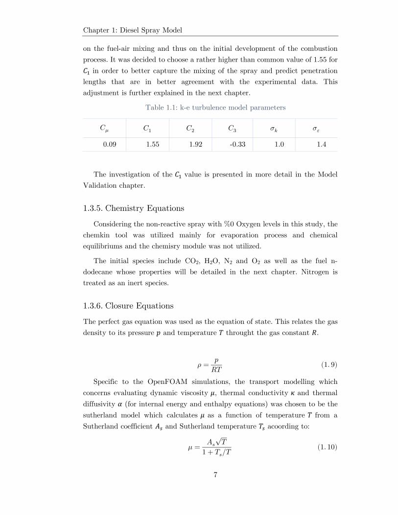
It was decided to choose a rather higher than common value of 1.55 for in order to better capture the mixing of the spray and predict penetration lengths that are in better agreement with the experimental data.
Lagrangian phase
In this approach the droplets are treated as individual mass points or computational parcels. A number of these computational parcels are injected into the flow domain according to the rate of injection profile. The properties of each parcel including its position, velocity and temperature are determined for each timestep by solving the governing equations in a lagrangian way. This ineraction between the two phases is modeled by a coupling scheme which allows for exchange of momentum in form of droplet velocity change, exchange of energy in form of heat and exchange of mass in form of droplet evaporation. The mass, momentum and energy equasions are described here in brief according to [11].
The mass equation for the droplet is as follows:
𝑑𝑚𝑑𝑑𝑡
= −𝑚𝑑𝜏𝑖
(8)
𝑑𝐷𝑑𝑡
= − 𝐷3𝜏𝑖
(9)
Where under standard evaporation and under boiling conditions. Droplet momentum
equation is defined as follows:
𝑚𝑑𝑑𝑢𝑑𝑑𝑡
= −𝜋𝐷2
8𝜌𝐶𝑑|𝑢𝑑 − 𝑢|(𝑢𝑑 − 𝑢) + 𝑚𝑑𝑔 (10)
The energy equation for the droplet is defined as follows and accounts for heat transfer and evaporation:
𝑚𝑑𝑑ℎ𝑑𝑑𝑡
= �̇�𝑑ℎ𝑣(𝑇𝑑) + 𝜋𝐷 𝜅 𝑁𝑢 (𝑇 − 𝑇𝑑) 𝑓 (11)
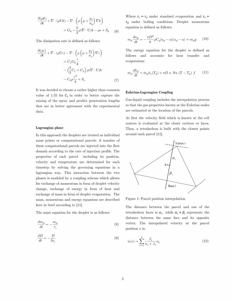
Eulerian-Lagrangian Coupling
Gas-liquid coupling includes the interpolation process so that the gas properties known at the Eulerian nodes are estimated at the location of the parcels.
At first the velocity field which is known at the cell centers is evaluated at the closet vertices or faces. Then, a tetrahedron is built with the closest points around each parcel [11].
i
i
Vertex i
Base i
x
Figure 1: Parcel position interpolation
The distance between the parcel and one of the tetrahedron faces is , while represents the distance between the same face and its opposite vertex. The interpolated velocity at the parcel position x is:
𝑢(𝑥) = ∑𝛽𝑖
𝛼𝑖 + 𝛽𝑖𝑢𝑖
4
𝑖=1 (12)

4
This method ensures that the parcels experience a continuous velocity field . The liquid-gas coupling is the effect of spray source terms on the Eulerian governing equations.
The Eulerian solution is frozen at time instant and the parcels are advanced one by one to the next time step of 𝑛 + 1 . All the source terms in the mass, momentum and energy equation are thus evaluated at the time 𝑛. Each parcel is tracked along its path by using the face-to-face algorithm. This makes possible to identify all the cells crossed by each parcel during one time step and to split the Lagrangian source terms of the Eulerian equations accordingly. If the velocity of the parcel is lower than the interpolated Eulerian velocity it will gain momentum which is taken from the Eulerian phase and reduce the Eulerian velocity. The droplet temperature, however, is not obtained by means of interpolation on the Eulerian phase. Instead, the energy equation accounts for heat transfer and evaporation of the droplets.
Every parcel is injected from a point located in a disk whose size is equal to the injector nozzle and the points are randomly chosen according to a uniform distribution. The frequency of the addition of new parcels is directly related to the fuel injection rate (ROI), assuming constant density of the liquid fuel and ideally spherical droplets. Following the blob injector model, every injected parcel is characterized by the same diameter which is comparable to the size of the nozzle hole on the gas side.
𝑁(𝑡) = 𝑚𝑎𝑥(1, 𝛥𝑡 𝑁𝑡𝑜𝑡𝑡𝑒𝑜𝑖 − 𝑡𝑠𝑜𝑖
) (13)
is the total number of parcels. There was an attempt to increase the total number of injected Parcels to around 100,000 but due to instabilities in the runtime this number was reduced to 30000. and indicate the time of end and start of injection respectively.
Blob - KH/RT model
The blob method is used as the injection model. This method is based on the assumption that atomization and drop break-up within the dense spray near the
nozzle are indistinguishable processes, and that a detailed simulation can be replaced by the injection of big spherical droplets with uniform size, which are then subject to secondary aerodynamic-induced break-up. The diameter of these droplets are assumed to be equal to that of the injector hole [14].
Figure 2: Schematics of the blob injection method
Determining the number of blobs based on the rate of injection and the speed and direction of the injection.
𝑈𝑏 =�̇�𝑖𝑛𝑗𝑒𝑐𝑡𝑖𝑜𝑛
𝐴𝑛𝑜𝑧𝑧𝑙𝑒. 𝜌𝑓
(14)
The direction of the blob is chosen to be a random angle within the spray cone. The blobs lose mass as they penetrate the spray
The KH model developed by Reitz and Diwakar [22] is based on a first order linear analysis of a Kelvin-Helmholtz instability growing on the surface of a cylindrical liquid jet with initial diameter . The new droplet continuously loses mass as it penetrates the gas and the rate of this shrinkage is related to how far the radius is from equilibrium radius (or the new child radius) and also the characteristic time span value.
𝑑𝑟𝑑𝑡
= − 𝑟 − 𝑟𝑛𝑒𝑤𝜏𝑏𝑢
(15)
𝜏𝑏𝑢 = 3.788 ⋅ 𝐵1𝑟
𝛬 ⋅ 𝛺 (16)
𝐵1 is an adjustable model constant including the influence of the nozzle hole flow like turbulence level and nozzle design on spray break-up. Values between 𝐵1=1.73 to 𝐵1=60 have been suggested.

5
The KH model, based on the work of Taylor [23], deals with the instability of the interface between two fluids of different densities in the case of an acceleration (or deceleration) normal to this interface.
𝛬 = 𝐶32𝜋√3𝜎
𝑎(𝜌𝑙 − 𝜌𝑔) (17)
𝐶3 is the adjustable constant used to allow modification of effective wavelength similar to B1 in KH model. Break-up time is found to be the reciprocal of the frequency of the fastest growing wave after which the drop disintegrates completely into small droplets of 𝑑𝑛𝑒𝑤 = 𝛬.
In the case of the KH-RT model, both models are implemented in CFD codes in a competing manner. Both models are allowed to grow unstable waves simultaneously, and if the RT-model predicts a break-up within the actual time step, the disintegration of the whole drop according to the RT mechanism occurs. Otherwise the KH model will produce small child droplets and reduce the diameter of the parent drop.
Figure 3: Catastrophic breakup schematics in KH/RT model
Typically a breakup length is set so only KH stripping breakup occurs in that length . This is due to the fact that reduction of droplet size by the RT model is too fast. After that the KHRT model is fully applied
in a competing manner and droplets break up for whichever conditions of KH or RT that applies.
Figure 4: Combined blob-KH/RT model
Pressure and Velocity coupling
The algorithm used in this project is a PIMPLE algorithm which is a coupling of SIMPLE and PISO algorithms [27]. This algorithm utilizes an inner PISO loop with the addition of an outer correction loop which includes cycling over the same time step using the previous iteration result as initial guess for next iteration.
Performance Indexes
A number of measurements were the focus of each CFD simulation in order to assess the simulation results and provide a basis for comparison. In Lib-ICE, the liquid length evolution as function of time is stored in a file named sp99.Bomb. It is defined as the axial distance from the injector where 99% of the liquid mass was found, which is the definition which is mostly used for comparison with experimental data of liquid spray penetration.
The steady state liquid length was defined as the average of the sp99 values from 0.45 ms to 1.2 ms. This threshold was observed to be well after the initial ramp up and able to filter out all the inherent noise in the values of sp99.
As for the vapor phase penetration in the OpenFOAM library, the fuel vapor penetration evolution as function of time is stored in a file named vapPen1.Bomb. It is defined as the maximum axial

6
distance where a mixture fraction value of 1e-3 was found. This is the definition which is currently used for comparison with experimental data of fuel vapor penetration.
Another important index is the spray mixing line. As the enthalpy balance for the mixture is expressed in terms of the following adiabatic mixing process [36].
ℎ(𝑇 ) = 𝑍. ℎ𝑓(𝑇0) + (1 − 𝑍). ℎ𝑎(𝑇𝑎) (18)
In order to investigate and ensure that the spray simulation is of the mixing limited evaporation nature, the mixture fraction at the location of the injected parcels is compared to the local temperature in the vicinity of the parcel to generate the mixing line.
Thus the ideal spray simulation is that which exhibits a tight mixing line with very low dispersion showing the closer to ambient temperature values as the mixture fraction is reduced. Other effects such as the heat transfer phenomena especially close to the injection nozzle could alter this line and cause dispersions as represented in Figure 5.
Z [%]
T[K
]
Figure 5: schematic of an ideal mixing limited spray mixing line
Higher 𝐵1 value leads to reduced break-up and increased penetration and a lower 𝐵1 value results in increased spray disintegration, faster fuel-air mixing, and reduced penetration.
This value requires careful tuning and adjustment for a balanced simulation of the spray.
Target Sprays
The sprays and their respective operating conditions simulated in this study are those denoted by ECN and the main focus of ECN5 workshop. The geometrical and operational details are denoted in the full report.
Grid Convergence
A collection of experimental geometry measurements for Spray A has led to the generation of educated 3D surface files, smoothed to remove experimental artifacts and provided through ECN. However, in the simulations conducted for this report, the focus was on a simplified wedge type mesh which was created in OpenFOAM using the blockMesh method. The 3D mesh file was only used for calculations of geometric ratios of the injector and cross checking with similar studies on Spray A. The wedge type domain is schematically presented in the following figure where a small slice of the cylinder with an angle less than 5 degrees is considered
Figure 6: Schematics of the Wedge type domain
The optimal grid sizing configurations were defined based on two principals: Mesh size and Mesh grading. Three options were chosen for each of these two parameters and the grading was set so the mesh would be much finer closer to the spray region where finer mesh resolution might be needed to capture the flow phenomena properly. This is both due to the injection causing great gradients near the nozzle region as well as the Lagrangian field of parcels being injected in the flows

7
Figure 7: Effect of grid size on liquid penetration
Figure 8: Effect of grading of grid size on vapor penetration
It is observed that the results of CFD simulation exhibit a convergence with respect to increasing the grid size for a same grading scheme and making the grid even finer will not be beneficial in terms of achieving better results and will simply bring about too much computational cost.
Figure 9: Effect of grid sizing on liquid length
Figure 10: Effect of grid sizing on mixture fraction at 30 mm
With a sizing of 0.127 mm for the smallest division and 23328 cells, the mesh proved to be reliable for the CFD setup capturing the penetration values and mixture fraction curve in a suitable fashion and with adequate resolution.
0
0.002
0.004
0.006
0.008
0.01
0.012
0.014
0.016
0.018
Liquid Pen
etration [m
]
time [s]
1458
5832
23328
36450
52488
0
0.01
0.02
0.03
0.04
0.05
0.06
Vap
or Pen
etration [m
]
time [s]
1458
5832
23328
36450
52488
0
0.002
0.004
0.006
0.008
0.01
0.012
0.014
Steady State Liquid Len
gth [m
]
Number of Cells

8
Turbulence Model Calibration
The k-ε model is widely used in CFD simulations to simulate mean flow characteristics for turbulent flow conditions. However, the values of the model constants are typically chosen to be in agreement with results of numerous iterations of data fitting for a wide range of turbulent flows. One important constant is the coefficient used in the dissipation (ε) equation.
Following the poor results of previous simulations with respect to mixing of the spray, the idea was to increase this parameter in order to simulate a more turbulent flow resulting in improved mixing of the spray and better agreement with experimental data.
The following figure shows the effect of increasing the 𝐶1 value on the liquid length evolution over time.
Figure 11: effect of C1 value on liquid penetration
Vapor penetration was exceedingly higher for higher 𝐶1 values. Considering the experimental data, it was decided to choose a rather higher than common value of 1.55 for 𝐶1 . Going even higher than the 1.55 threshold was considered to cause unrealistic turbulent simulation results and further case tuning of other influential parameters was a more rational approach than to improve the penetration results by merely increasing the 𝐶1 value to even higher unrealistic quantities.
Figure 12: Effect of 𝐶1 value on vapor penetration
The final turbulence model parameters are tabulated below which are
Table 1: k-e turbulence model parameters
𝐶𝜇 𝐶1 𝐶2 𝐶3 𝜎𝑘 𝜎𝜀
0.09 1.55 1.92 -0.33 1.0 1.4
Additionally the effect of turbulent Schmidt number on penetration values was studied. Conceptually, this value is the ratio of eddy viscosity to eddy diffusivity of the flow and describes the ratio between the rates of turbulent transport of momentum and the turbulent transport of mass.
(15)
There appears to be no significant change in vapor penetration simulation results. This is in agreement with other studies suggesting that the turbulent Schmidt number has minor impact on such simulations [44]. The value of 1.0 was chosen to be used and this was in agreement with the range of Schmidt numbers used in similar simulations [45, 46].
0
0.002
0.004
0.006
0.008
0.01
0.012
0.014
0.016
0.018
Liquid Pen
etration [m
]
time [s]
1.44
1.52
1.55
1.6
SNL 675
0
0.01
0.02
0.03
0.04
0.05
0.06
Vap
or Pen
etration [m
]
time [s]
1.44
1.52
1.55
1.6
SNL 675

9
Figure 13: Effect of turbulent Schmidt number on liquid penetration
Figure 14: Effect of turbulent Schmidt number on vapor penetration
In a variety of previous ECN workshops, Schmidt numbers close 0.9 has been adopted [47].
Results and Discussion
After the case tuning procedure, the proper simulation parameters were identified in order to exhibit the best matching with the SNL experimental data for the Spray A675 standard condition. The final CFD model is summarized in the following table:
Table 2: Summary of Final Simulation parameters
Parameter Description
Software used OpenFOAM, Lib-ICE library
Turbulence model with 1.55
Turbulent Schmidt number 1.0
Sub-grid or turbulent scalar transport
Gradient Transport
Spray Model Lagrangian discrete phase model
Injection Blob
Atomization and Breakup KHRT with breakup length
Collision None
Drag Spherical Drag Model
Evaporation Spalding
Heat Transfer Ranz-Marshall
Dispersion None
Injection Pressure 150MPa
Ambient density 22.8 kg/m^3
Ambient Pressure for 900
6MPa
Table 3: Final Grid Details
Dimensionality 2D axisymmetric Wedge
Type Block structured
Grid size range (mm) 0.127 mm – 1.27 mm
Total grid number 23328 Cells
0.000
0.002
0.003
0.005
0.006
0.008
0.009
0.011
0.012
0.014
0.015
0.017
0.018
Liquid Pen
etration [m
]
time [s]
0.5
0.8
0.9
1.0
1.2
0
0.01
0.02
0.03
0.04
0.05
0.06
Vap
or Pen
etration [m
]
time [s]
0.5
0.8
0.9
1.0
1.2

10
Table 4: Time advancement method details
Time discretization scheme
PIMPLE
Fixed time-step (sec) 2e-7 with max Courant number of
0.25
Table 5: Breakup and atomization parameter details
B0 0.61
B1 40
Ctau 1.0
CRT 0.1
msLimit 0.02
WeberLimit 6
cBU 12
For the standard condition, the simulation results are presented. At first the penetration values is examined for both liquid length and vapor penetration. The following figure shows the evolution of penetration values through time as well as the experimental data available from SNL.
The simulation shows quite good agreement with experimental values of liquid and vapor penetration for the standard condition. It should be noted that other sets of parameters would lead into a better capturing of the vapor penetration value but that required pushing some constants such as the 𝐶1 value to extreme measures and it was decided to avoid that approach.
Figure 15: Penetration results for standard condition spray A
Figure 16: Mixing line for Spray A at standard condition
0.00
0.01
0.02
0.03
0.04
0.05
0.06
Pen
etration [m
]
time [s]
Simulation Liquid Length
Simulation Vapor Penetration
SNL 675 Liquid Length
SNL 675 Vapor Penetration
𝑉𝑎𝑝𝑜𝑟 𝑃𝑒𝑛𝑒𝑡𝑟𝑎𝑡𝑖𝑜𝑛
𝐿𝑖𝑞𝑢𝑖𝑑 𝑃𝑒𝑛𝑒𝑡𝑟𝑎𝑡𝑖𝑜𝑛

11
The spray line exhibits low dispersion in this case indicating a proper mixing spray simulation. The tuning of breakup parameters has resulted in proper matching with the Sandia experimental data for steady state liquid penetration of 11.7mm.
Ambient Temperature Effect
To test the model’s fidelity and robustness, ECN denotes a number of conditions that involve various ambient temperatures. For fixed ambient density values, the ambient temperature was increased from 700K to 1200K.
The following figure shows liquid and vapor penetration data for Spray A at 700K.
Figure 17: Liquid and Vapor penetration results for Spray A at T=700K
The experimental data available for this specific injector and injection condition form SNL are also represented. It can be observed that the model, specifically tuned for T=900K is not capable of
capturing the liquid length properly at lower temperatures while it still predicts the vapor penetration in a suitable margin of error. The lower temperature simulations is particularly challenging due to less temperature difference between the fuel and the ambient gas and the evaporation is less promoted resulting in higher liquid length prediction of 22 mm which is way above the experimental values of around 18
Figure 18: Mixing line for Spray A at T=700k
The following figure shows an overlapping of liquid and vapor penetration lines for the study of the ambient temperature’s effect on the model.
It can be observed that the liquid length simulation is quite sensitive to ambient temperature. The average liquid length is progressively reduced for higher ambient temperature values whereas the vapor penetration line, although changed slightly to lower values, does not seem to be affected as much. Other interesting observation is the jitter in the liquid length line that involved a higher amplitude for the T=700K case.
0
0.01
0.02
0.03
0.04
0.05
0.06
Pen
etration [m
]
time [s]
Simulation Liquid Length
Simulation Vapor Penetration
SNL 675 Liquid Length #1
SNL 675 Liquid Length #2
SNL 675 Vapor Penetration
𝑉𝑎𝑝𝑜𝑟 𝑃𝑒𝑛𝑒𝑡𝑟𝑎𝑡𝑖𝑜𝑛
𝐿𝑖𝑞𝑢𝑖𝑑 𝑃𝑒𝑛𝑒𝑡𝑟𝑎𝑡𝑖𝑜𝑛

12
Figure 19: Effect of ambient temperature on penetration values
Figure 20: Ambient temperature effect on simulation results
The experimental data are from Sandia National Laboratories and CMT-Motores Térmicos and they indicate the model over predicts the steady state liquid penetration at lower Temperatures. This is
corroborated with the disperse spray line as presented above.
Similar study of liquid penetration was also conducted on Spray C and D. Due to lack of experimental results available for the target sprays (D134 and C003), in this case the experimental data for other injector numbers of the same kind was used. Namely the D134 and C037.
Figure 21: Experimental and simulation results for Spray D
The red bars in this figure show the range of the available experimental data.
For Spray D134, the one instance of available experimental result for 900 shows promising agreement with the simulated value of 25 mm for liquid length. Same cannot be said for the spray D135. Although the trend shows agreements with the experimentations but the error margin appears to be high. The value of 1.0 was used for Spray D as cavitation was not expected.
700K 800K 900K 1000K 1100K 1200K
0
0.01
0.02
0.03
0.04
0.05
0.06
Pen
etration [m
]
time [s]
600 800 1000 1200 1400
0.0000
0.0050
0.0100
0.0150
0.0200
0.0250
T [K]
Average Liquid Pen
etration [m]
Simulation Experimental
800 900 1000 1100
0
0.005
0.01
0.015
0.02
0.025
0.03
0.035
0.04
T [K]Average Liquid Pen
etration [m]
Sim D135 Exp D135
Exp D134 Sim D134
𝑉𝑎𝑝𝑜𝑟 𝑃𝑒𝑛𝑒𝑡𝑟𝑎𝑡𝑖𝑜𝑛
𝐿𝑖𝑞𝑢𝑖𝑑 𝑃𝑒𝑛𝑒𝑡𝑟𝑎𝑡𝑖𝑜𝑛

13
Figure 22: Experimental and simulation results for Spray C
For Spray C, according to a previous ECN4 study, a value of 0.81 was used and this proved to be in
good agreement with the experimental results for C003 but the same cannot be said for C037.
Nonetheless, the study of spray C and D is a good indication of the fidelity of the simulation and applicability of its results in various conditions.
The simulation results was submitted as part of the contributions for the third topic of ECN5 workshop as an evaporative spray simulation. Other contributions incorporated different CFD setup and simulation approach including the utilization of DNS and LES simulations. The investigation of simulation result discrepancies as well as the points of agreement highlighted the more challenging areas for simulations and the aspects which tend to show more deviation from experimental results are highlighted.
Focusing on the macroscopic features of the spray, the next figure shows the simulation results for the average liquid length at various ambient temperatures. The liquid penetration results shows that various spray simulations struggle most at the lower temperature levels and mostly under predict it.
Figure 23: Liquid penetration results of ECN5
Figure 24: Mixing Line results of ECN5
Comparing the mixing line between the various submissions reveals some interesting characteristics. The 1D adiabatic mixing model results are shown in the form of a dashed line as reference. The scatter plot for various submissions is also presented. An interesting phenomena is the so called “knee” in the mixing line where the data seems to shift backwards. Politecnico and TUM results exhibited this trait at slightly richer mixtures as opposed to CMT results. The Temperature at which the “knee” is observed is rather significant as the temperatures above that threshold (close to 570K) are associated with only the gas phase while below that level both liquid and gas phase are present in the corresponding cell.
800 900 1000 1100
0
0.005
0.01
0.015
0.02
0.025
0.03
0.035
0.04
T [K]
Average Liquid Pen
etration [m]
Sim C003 Exp C003
Exp C037 Sim C037

14
One motivation in the reason behind different simulation result for this temperature level could be non-identical fuel properties as well as various methods used to calculate the temperature. Nonetheless, this effect could be the focus of future work.
Figure 25: Mixture fraction as function of axial distance. ECN5
Mixture fraction at various axial locations is another interesting comparison in the data as it exposed another measurement where many simulations seemingly were in agreement except for one (RWTH). This difference is also observed one the mixture fraction is plotted at a fixed axial position as presented in the following figure.
RWTH simulation involves a DNS simulation close to nozzle and LES model for further downstream. Their model seems to be under predicting the mixture fraction compared to other data but it should be noted that it captures the regions with lower mixture fraction with better agreement to experimental data as presented in the following figure.
Figure 26: Mixture fraction at axial position of 30 mm
In other comparisons it was observed that all simulations are over predicting the velocity prior to the axial distance of 18-20 mm after which there seems to be good agreement between the simulation and experimental data. It appears that RANS models have an advantage in predicting the velocity profiles farther from the nozzle. The difference is more pronounced for the peak velocity values.
Conclusions
A direct injection diesel spray was simulated using a RANS model by means of a Lagrangian-Eulerian approach.
Steady state liquid penetration and vapor phase penetration were selected as the main injector simulation indexes as well as the spray shape visualization using the Lagrangian field and a definition of the spray mixing line was introduced. Parameters of standard - turbulence model, turbulent Schmidt number and the computational grid were studied for their impact on simulation results and modified to better capture the spray phenomena and mixing. Additionally, the blob injection model and a KH/RT breakup model was adopted and the parameters were tuned to match the experimental results of SNL available at Spray A standard conditions.

15
The same simulation was applied to different injection conditions at various temperatures keeping the same ambient density to observe the effect of ambient temperature on the results. It was observed that the steady state liquid penetration is reduced for higher ambient temperatures where spray evaporation is facilitated. The correlation between mixing line dispersion and validity of simulation results was demonstrated. The simulation results appear to be in good agreement with the experimental data above ambient temperatures of 900K below which the model over predicts the steady state liquid length and exhibits an observable dispersion in the mixing line.
Furthermore, same Spray A simulation parameters were used to simulate Spray C and D conditions with higher nominal nozzle diameter than Spray A and different nozzle shape more prone to flow cavitation inside the nozzle hole. Simulation results show considerable variation form the experimental results and the liquid length was not reliably captured for spray C.
The results were presented as contribution to the fifth ECN workshop along with contribution of other institutions and groups for the third topic of the workshop regarding non-reactive diesel spray mixing and evaporation. The discrepancies in the simulation results shows the sensitivity of such simulations to the models embedded and the simulation parameters.
Most simulations predict the liquid length of the Spray A with good accuracy but the uncertainty in the experimental data makes this comparison more difficult. The liquid length seems to be under predicted at lower temperature levels for most simulation results but at higher temperature levels the results are in better agreement with experimentations. As for the vapor phase penetration, the simulation results show better consistency regardless of the model used and better results are obtained also for lower temperature values. With respect to other measurements such as mixture fraction or velocity field at various axial distances from the nozzle, there appears to be variability between the predictions of different models. This discrepancy is more pronounced if we focus our attention to the jet front as opposed
to the entire spray global features and it appears that the averaging schemes of RANS and LES provide different predictions with respect to variables such as the mixture fraction. Simulations of Spray C and D were able to predict the difference in penetration values and distinguish between the two sprays but they showed considerable margins of error with respect to experimental data.
Considering the future work on this topic, it appears that focusing on macroscopic features of the spray such as liquid length and vapor phase penetration does not provide a good picture of the simulation accuracies. Despite the attention to spray mixing line, other indexes could be interesting in model tuning. Some motivations based on simulation results of this work as well as previous ECN workshops include examining the SMD values at certain axial distances and a focus on model tuning for lower temperatures. As for Spray C and D, the involved cavitation could call for a modified atomization approach and further study of those specific sprays and performing case tuning could prove beneficial.
Acknowledgement
I would like to thank Professor Tommaso Lucchini, the thesis advisor at Politecnico di Milano without whom this work would not have been possible. I would also like to show my gratitude to Dr. Michele Bardi who was the organizer for the third topic in the ECN5 workshop for providing the information and part of the experimental data pertaining to this work as well as his presentation of the results as a contribution to the workshop.
Bibliography
Please refer to the full report for the full list of references. The numbering scheme is consistent between the two.

I
This page is intentionally left blank
II
Acknowledgements
I would like to thank all the people who were my inspiration and their support made this work possible. First I’d like to thank Professor Tommaso Lucchini, my dear advisor at Politecnico di Milano who was always available and whose deep knowledge of the topic and passion was a fantastic motivation and guide.
I also would like to thank Mr. Davide Paredi and the PHD team of the ICE department of Politecnico di Milano who always had a positive attitude towards issues and were quite welcoming. I would like to also show my gratitude to Dr. Michele Bardi who was the organizer of the third topic in the ECN5 workshop for providing the information and part of the experimental data pertaining to this work as well as his presentation of the results as a contribution to the ECN5.
Last and certainly not least I would like to thank my amazing friends and my fantastic family for filling my life with love and compassion and motivating me to go the extra distance.

III
Table of Contents
Introduction .................................................................................................. 1
1. Diesel Spray Model ............................................................................... 3
1.1. Background .................................................................................... 3
1.2. Governing Equations ..................................................................... 4
1.3. Eulerian Phase ............................................................................... 4
1.3.1. Continuity equation ................................................................ 4
1.3.2. Momentum Equation .............................................................. 5
1.3.3. Energy Equation ..................................................................... 5
1.3.4. Turbulence Equation .............................................................. 6
1.3.5. Chemistry Equations ............................................................... 7
1.3.6. Closure Equations ................................................................... 7
1.4. Lagrangian Phase .......................................................................... 8
1.4.1. Mass Equation ........................................................................ 8
1.4.2. Momentum Equation .............................................................. 9
1.4.3. Energy Equation ..................................................................... 9
1.5. Atomization ................................................................................. 10
1.5.1. Blob Injection Model ............................................................. 10
1.5.2. Kelvin-Helmholtz Breakup Model ......................................... 11
1.5.3. Rayleigh-Taylor Break-up Model .......................................... 13
1.5.4. Combined Break-up Model ................................................... 14
2. OpenFOAM and Lib-ICE ................................................................... 16
2.1. CFD Model .................................................................................. 17
2.1.1. OpenFOAM setup ................................................................. 17
2.2. Numerical Schemes ...................................................................... 18
2.2.1. Equation discretization ......................................................... 18

IV
2.2.2. Temporal Discretization ........................................................ 20
2.2.3. Summary ............................................................................... 21
2.3. Eulerian-Lagrangian Coupling ..................................................... 21
2.3.1. Gas-Liquid Coupling ............................................................. 21
2.3.2. Liquid-Gas Coupling ............................................................. 22
2.4. Pressure and Velocity Coupling .................................................. 23
2.5. Computational Grid .................................................................... 23
2.6. Performance Indexes .................................................................... 24
2.6.1. Liquid Length ........................................................................ 25
2.6.2. Jet Penetration ..................................................................... 25
2.6.3. Spray Mixing Line ................................................................. 26
2.6.4. Spray Shape .......................................................................... 28
2.7. Simulation Parameters ................................................................ 29
2.8. Post Processing ............................................................................ 30
2.8.1. Automation Scripts ............................................................... 30
3. Model Validation ................................................................................ 32
3.1. Spray case study .......................................................................... 32
3.1.1. SNL Experimental Setup ...................................................... 33
3.1.2. Spray Characteristics ............................................................ 36
3.1.3. Rate of Injection ................................................................... 38
3.1.4. Target Sprays ........................................................................ 40
3.2. Target Conditions ........................................................................ 41
3.3. Experimental Parameters ............................................................ 42
3.4. Grid Convergence ........................................................................ 44
3.5. Turbulence Model Calibration ..................................................... 49
3.6. Effects on Spray Mixing Line and Penetration ........................... 53
4. Results and Discussion ....................................................................... 56
4.1. Standard Condition ..................................................................... 58
4.2. Ambient Temperature Effect ....................................................... 62

V
4.3. Spray C and D simulation ........................................................... 67
4.4. ECN5 Submissions ....................................................................... 69
Conclusions ................................................................................................. 74
Bibliography ............................................................................................... 76

VI
List of Figures
Figure 1.1: Schematics of the blob injection method ................................. 11
Figure 1.2: Kelvin-Helmholtz model ........................................................... 12
Figure 1.3: Rayleigh-Taylor instability ...................................................... 14
Figure 1.4: Catastrophic breakup schematics in KH/RT model ................ 15
Figure 1.5: Combined blob-KH/RT model ................................................. 15
Figure 2.1: Parameters in finite volume discretization ............................... 18
Figure 2.2: Parcel position interpolation .................................................... 22
Figure 2.3: Schematics of the Wedge type domain .................................... 24
Figure 2.4: 3D schematic of the Wedge type geometry .............................. 24
Figure 2.5: Schematics of the penetration values over time ....................... 26
Figure 2.6: schematic of an ideal mixing limited spray mixing line ........... 27
Figure 2.7: Schematics of the dispersion of the spray mixing line ............. 27
Figure 2.8: Schematics of the diesel spray .................................................. 28
Figure 3.1: Optically accessible constant volume SNL spray chamber ...... 33
Figure 3.2: The SNL vessel shcematic ........................................................ 33
Figure 3.3: The Combustion Chamber ....................................................... 34
Figure 3.4: Chamber Volume Schamatics .................................................. 35
Figure 3.5: Half and full 3D chamber view ................................................ 36
Figure 3.6: ROI for Spray C with Injection Pressure of 50MPa ................ 40
Figure 3.7: X-ray tomography of nozzle D (left) and C (right) ................. 41
Figure 3.8: Mesh simple grading along a block edge .................................. 44
Figure 3.9: Finer mesh closer to the Spray ................................................ 44
Figure 3.10: Simple grading scheme near the nozzle outlet ........................ 45
Figure 3.11: Effect of grid size on liquid penetration ................................. 46
Figure 3.12: Effect of grading of grid size on vapor penetration ................ 46

VII
Figure 3.13: Effect of grid sizing on liquid length ...................................... 48
Figure 3.14: Effect of grid sizing on mixture fraction at 30 mm ................ 49
Figure 3.15: effect of C1 value on liquid penetration .................................. 50
Figure 3.16: Effect of 𝐶1 value on vapor penetration ................................ 51
Figure 3.17: Effect of turbulent Schmidt number on liquid penetration .... 52
Figure 3.18: Effect of turbulent Schmidt number on vapor penetration .... 52
Figure 3.19: Effect of increasing the 𝐵1 value on the mixing line ............. 53
Figure 3.20: Lagrangian Field and Mean Void Fraction ............................ 54
Figure 3.21: Spray Mixing Line .................................................................. 54
Figure 3.22: Effects of increasing CRT and Ctau values on penetration ... 55
Figure 4.1: Penetration results for standard condition spray A ................. 58
Figure 4.2: Simulation details for the standard condition Spray A ........... 59
Figure 4.3: Mixing line for Spray A at standard condition ........................ 59
Figure 4.4: Spray A evolution over time under standard conditions ......... 61
Figure 4.5: Liquid and Vapor penetration results for Spray A at T=700K 62
Figure 4.6: Simulation details for Spray A at T=700K ............................. 63
Figure 4.7: Mixing line for Spray A at T=700k ......................................... 63
Figure 4.8: Effect of ambient temperature on penetration values .............. 64
Figure 4.9: Simulation details of Spray A at higher temperatures ............. 66
Figure 4.10: Ambient temperature effect on simulation results ................. 67
Figure 4.11: Experimental and simulation results for Spray D .................. 68
Figure 4.12: Experimental and simulation results for Spray C .................. 68
Figure 4.13: Liquid penetration results of ECN5 topic 3 ........................... 70
Figure 4.14: Mixing Line results of ECN5 topic 3 ...................................... 71
Figure 4.15: Mixture fraction as function of axial distance. ECN5 ............ 72
Figure 4.16: Mixture fraction at axial position of 30 mm .......................... 72
Figure 4.17: Velocity profile at various axial positions .............................. 73
Figure 4.18: Velocity profile at axial position of 30 mm ............................ 73

VIII
List of Tables
Table 1.1: k-e turbulence model parameters ................................................ 7
Table 2.1: Numerical schemes for the divergence terms used .................... 21
Table 2.2: Numerical schemes for the other terms used ............................. 21
Table 3.1: Spray A specifications and operating conditions ....................... 36
Table 3.2: Geometric details of Spray A .................................................... 40
Table 3.3: Spray conditions simulated for ECN5 ....................................... 42
Table 3.4: n-dodecane Properties ............................................................... 43
Table 4.1: Summary of Final Simulation parameters ................................ 56
Table 4.2: Final Grid Details ..................................................................... 57
Table 4.3: Time advancement method details ........................................... 57
Table 4.4: Breakup and atomization parameter details ............................. 57
Table 4.5: Summary of ECN5 participants ................................................ 69

IX
Abbreviations
ASI After Start of Injection CFD Computational Fluid Dynamics CN Cetane Number DDM Discrete Droplet Model DI Direct Injection DNS Direct Numerical Simulation ECN Engine Combustion Network EGR Exhaust-Gas Recirculation EOS Equation of State ICE Internal Combustion Engine KH Kelvin-Helmholtz Model LES Large Eddy Simulation Nu Nusselt Number PDE Partial Differential Equation PISO Pressure Implicit with Splitting Operators Pr Prandtl Number RANS Reynolds Averaged Navier Stokes Re Reynolds Number RT Rayleigh-Taylor Model Sc Schmidt Number Sh Sherwood Number SIMPLE Semi-Implicit Method for Pressure-Linked Equations SMD Sauter Mean Diameter SNL Sandia National Laboratories SOI Start of Injection VLE Vapor-Liquid Equilibrium We Weber Number Z Ohnesorge Number

X
𝛼 Thermal diffusivity for enthalpy Turbulent thermal diffusivity
Δ Difference [ / ]
Dissipation rate of turbulent kinetic energy [𝑚2/𝑠3]
energy ratio [ / ]
Λ Wave Length of Fastest Growing Wave [𝑚]
Dynamic Viscosity [(𝑁 𝑠)/𝑚2 ]
Kinematic Viscosity [𝑚2/𝑠] Density [𝑘𝑔/𝑚3 ]
Characteristic Time Scale [𝑠] , Shear Stress [𝑁/𝑚2]
Φ Spray Cone Angle [rad], [𝑑𝑒𝑔]
Growth Rate [𝑠−1 ]
Ω Growth Rate of Most Unstable Wave [𝑠−1]
𝐴 area [𝑚2]
𝐶𝑐 contraction coefficient [ / ]
𝐶𝑑 discharge coefficient [ / ]
𝐶𝐷 drag coefficient [ / ]
𝑐𝑝 specific heat capacity at constant pressure [𝐽/(𝑘𝑔 𝐾)] 𝑐𝑣 specific heat capacity at constant volume [𝐽/(𝑘𝑔 𝐾)] 𝑑 diameter [𝑚],
𝐷 nozzle hole diameter [𝑚],
ℎ Enthalpy [𝐽/𝑘𝑔]
𝐿 Length of nozzle hole [𝑚]
𝑚 mass [𝑘𝑔]
𝑝 Pressure [𝑃𝑎]
𝑅 Gas constant [𝐽/(𝑘𝑔 𝐾)] 𝑟 Radius [𝑚]
𝑆 Source term
𝑡 Time [𝑠] 𝑇 Temperature [𝐾]
𝑇𝑠 Sutherland Temperature [𝐾]
𝑢 velocity component [𝑚/𝑠] U Velocity [𝑚/𝑠] 𝑌 mass fraction in gas phase [ / ]

XI
Abstract
Computational methods have been an indispensable tool in rapid engine design and improvement. Difficulties in direct experimental measurements of the optically thick liquid core in the diesel fuel injection, which occurs at high temporal and spatial resolutions, has resulted in various breakup models and methods to describe the injection physics.
This work focuses on Eulerian-Lagrangian CFD simulation of the fuel injection inside the diesel combustion chamber in non-reactive conditions using Lib-ICE, an OpenFOAM Library. The model was tuned so that the simulation results were in agreement with the results of experimental data with regards to parameters such as liquid and vapor penetration and the spray mixing line. The case tuning involved turbulence model coefficient adjustment, turbulent Schmidt number modification and adjusting the parameters regarding a blob-KH/RT breakup scheme. Simulation fidelity with respect to ambient gas temperatures as well as simulating various spray nozzles was examined and discussed. The results was presented as contribution to the fifth ECN workshop under the third topic regarding evaporative spray simulation.
Keywords: CFD, OpenFOAM, Lib-ICE, Diesel, non-Reactive Spray, breakup, KH/RT, ECN, Mixing Line

1
Introduction
Introduction
Liquid spray simulation concerns a wide range of natural phenomenon present in a variety of technical systems and industrial applications. One of the main area of focus for this type of fluid simulation is the diesel sprays. Due to their reliability, better part load operation, fuel flexibility, etc. diesel engines have been widely adopted from medium-low to high power units [1, 2].
From an environmental perspective, the growing concerns on human caused global climate change [3] as well as the adverse health effects of exposure to gaseous and particulate components of vehicular emissions [4, 5] have been historically pushing the industry to lower the diesel engine emissions. Furthermore, the global energy demands have been calling for better fuel economy in modern engines and thus, the diesel engine has been undergoing a rapid development and refinement ever since its commercialization with the two main objectives of lowering engine emission levels, and preserving performance and improving fuel economy [6, 7]. Nevertheless, the relentless development of diesel engines in the last decades has been largely a consequence of the improvement of the injection systems performance and flexibility and the implementation of new combustion strategies [8].
The modern methods of fluid simulation have been a key factor in these rapid improvements over the years and have proved beneficial as opposed to conventional methods of prototyping since numerical simulation can be used to investigate processes that take place at time and length scales or in places that are not accessible and thus cannot be easily investigated using experimental techniques [2, 9]. This is crucial since there are many challenges associated with measuring diesel injection since spray breakup is characterized in the orders of micrometers and nanoseconds and the optically thick nature of the liquid core near the nozzle could introduce significant uncertainty in optical measurements [10]. By utilizing computational fluid dynamics (CFD) in conjunction with

Introduction
2
experiments in has been possible to drastically reduce the time and cost associated with diesel engine development [11].
This project was defined around the participation of Politecnico di Milano in the fifth edition of the Engine Combustion Network (ECN) workshop [12], on the topic of diesel spray mixing and evaporation. More specifically, it involved computational fluid dynamic simulation of the fuel injection inside the diesel combustion chamber in non-reactive conditions with a focus on three specific injectors dubbed Spray A,C and D. The non-reactive injection is simulated with the aim of better understanding the liquid core breakup and the subsequent formation of droplets and evaporation in the implemented method. The focus was on some of the most important parameters in diesel spray vaporization process i.e. the penetration length of liquid and vapor and the spray mixing line. The effects of various simulation parameters such as the breakup scheme coefficients and ambient temperature were studied.
An invaluable database of experimental tests conducted by various participating institutions in the ECN was utilized for simulation validation purposes and model tuning. The results were presented in the ECN5 workshop held at Wayne State University in Detroit, USA, along with the contributions from other participating institutions and groups.
The ECN is an international collaboration among experimental and computational researchers in engine combustion. The aim is to establish an internet library of well-documented experiments that are appropriate for model validation and the advancement of scientific understanding of combustion at conditions specific to engines. In this work, a CFD solver for combustion simulation in direct injection Diesel engines has been implemented in Lib-ICE, an OpenFOAM library for internal combustion engine simulations developed by the ICE group of Politecnico di Milano.
This work is organized in four chapters. First the spray model is discussed and the main equations governing the flow are presented. The second chapter focuses more on the CFD implementations in OpenFOAM and Lib-ICE and introduces the important simulation parameters. Third chapter deals with case tuning and correcting the CFD simulation with respect to available experimental results. The simulation results are presented in the fourth chapter and discussed. Finally, the main achievements of this work and most important findings are presented in the conclusions section.

3
1. Diesel Spray Model
Chapter 1 Diesel Spray Model
1.1. Background
The diesel spray involves very turbulent fluid flow with extreme gradients. With nozzle diameter scales of around 0.1 mm and nominal injection velocities of 200-400 m/s; Simulating this turbulent reacting flow has proven to be one of the most difficult problems of applied macroscopic physics [11].
The widespread adoption of Computational Fluid Dynamics (CFD) in diesel spray studies should come as no surprise as the extremely resolute temporal and spatial scales of the optically thick injection limit our understanding of the physics involved. Nevertheless the diesel spray is one of the most challenging flow phenomena to be simulated and many theories have been developed to describe the disintegration of the liquid core into droplets and subsequent evaporation of the fuel during the injection process. Early attempts at modeling the diesel spray run the gamut of utilizing highly empirical equations [13, 14] to use of continuity and momentum equations highly dependent on experimental results [15, 16]. With the growing appeal and accessibility of CFD simulations and their applications to engine development and design, a handful of injection models were developed that focus on characterizing fuel penetration within the combustion chamber [17]. These simulation have been maturing over the years and provide fundamental information about the injection process, often not available from the experiments or simply not attainable at desired detail or repeatability. In this chapter the governing equations and the breakup models used in this simulation are explained.

Chapter 1: Diesel Spray Model
4
1.2. Governing Equations
The governing equations of fluid mechanics completely determine the behavior of the flow phenomena and can be summarized as follows:
Continuity equation which deals with conservation of mass
Momentum equations which are attained by applying the law of conservation of momentum in each of the three Cartesian dimensions
Energy equation which ensures the conservation of energy
Typically these equations are referred to as the “Navier-Stokes” equations. Additionally an equation of state is used to determine the state of the fluid.
In short, CFD is solving these equations with the help of a computer through numerical methods on a geometrical domain divided into small volumes. One important distinction in case of the diesel injection is that in order to calculate a spray penetrating into the gaseous atmosphere of the combustion chamber, two phases, the dispersed liquid and the continuous gas phase, must be considered. The Eulerian formulation, while suitable for modeling of the continuous gaseous phase, is not appropriate for the description of the disperse liquid phase. In the following sections the Eulerian and Lagrangian phases are described in more details.
1.3. Eulerian Phase
The gas medium is treated in an Eulerian fashion and the spray evolves into the domain based on the mass, momentum and energy exchange with the continuous gas phase. For the gas phase, the mass, momentum and energy equations are solved for a compressible, multi-component gas flow using the RANS approach.
The equations are described in brief according to [11, 18].
1.3.1. Continuity equation Considering an infinitesimal flow element which is fixed in space, we can
obtain the continuity equation in conservation form by applying the mass conservation principal:
𝜕𝜌𝜕𝑡
+ ∇. (𝜌. U) = 𝑆�̇� (1. 1)

Chapter 1: Diesel Spray Model
5
Where denotes the density of the gas and U is the velocity vector field. is a source term related to largrangian apprach of spray simulation. Source terms in the conservation equations of the gas phase enable the increase or decrease of momentum, energy, and mass in each grid cell and in this case the exchange of mass between the Lagrangian phase and the Eulerian phase is considered through the source term.
The conservation of species mass fraction:
𝜕𝜌𝑌𝑖𝜕𝑡
+ 𝛻. (𝜌. U𝑌𝑖) − 𝛻. [(𝜇 + 𝜇𝑡)𝛻𝑌𝑖] = 𝑆�̇�,𝑖 + 𝑆�̇�ℎ𝑒𝑚,𝑖 (1. 2)
in this equation indicates the mass fraction of species i.
1.3.2. Momentum Equation Considering the momentum equation, applying the newton’s second law we
can obtain the momentum equations in conservation form in each of the three Cartesian directions as follows:
𝜕(𝜌U)𝜕𝑡
+ 𝛻. (𝜌UU) =
−𝛻𝑝 + 𝛻. [(𝜇 + 𝜇𝑡)(𝛻U + (𝛻U)𝑇 )] − 𝛻. [(𝜇 + 𝜇𝑡) (23 𝑡𝑟(𝛻U)𝑇 )] + 𝜌𝑔 + 𝑆�̇�(1. 3)
is the gas dynamic viscosity and is the turbulent viscosity of gas phase. The term tr denotes the trace operator on matrices; the trace of a matrix is the sum of its diagonal elements.
is a source term related to largrangian apprach of spray simulation. Also it should be noted that the gravitational acceleration was neglected in this study.
1.3.3. Energy Equation
As for the energy equation, it is derived from the first law of thermodynamics which states that the rate of change of energy of a fluid particle is equal to the rate of heat addition to the fluid particle plus the rate of work done on the particle. Adopting the sensible enthalpy form of the energy equation:
ℎ = ∑ 𝑌𝐾
𝑛𝑠
𝑘=1(𝛥ℎ𝑓,𝑘
0 + ∫ 𝐶𝑝𝑘𝑑𝑇
𝑇
𝑇0
) (1. 4)
With being the total number of species and be the mass fraction of the generic species k. is teh specific heat capacity at constant pressure and
Chapter 1: Diesel Spray Model
6
is a reference temperature.Δh , is the heat of formation of species k at the reference temperature. Finally, the energy equation can be expressed as follows:
𝜕(𝜌ℎ)𝜕𝑡
+ 𝛻. (𝜌Uℎ) − 𝛻[(𝛼 + 𝛼𝑡)𝛻ℎ] = 𝐷𝑝𝐷𝑡
+ 𝑆�̇� (1. 5)
𝛼 is the thermal diffusivity for enthalpy and 𝛼𝑡 is the turbulent thermal diffusivity.
All the source terms , , , and are present to account for mass, momentum and energy exchange between the gas and the liquid phases as will be discussed in the coupling section in the next chapter.
1.3.4. Turbulence Equation
Adopting a Reynolds Averaged Navier Stokes (RANS) model; The standard - model was used in this report for the modeling of turbulence in the spray
simulation. In this model, dynamic turbulent kinematic viscosity is defined as:
𝜇𝑡 = 𝜌𝐶𝜇𝑘2
𝜀1. 6
Turbulence kinetic energy and dissipation rate are obtained by the solution of their respective (or equivalent) transport equations.
The turbulent kinetic energy equation is given by:
𝜕 𝜌𝑘𝜕𝑡 + 𝛻 ⋅ 𝜌U𝑘 − 𝛻 ⋅ 𝜌 𝜇 +
𝜇𝑡𝜎𝑘
𝛻𝑘 = 𝐺𝑘 −23 𝜌 𝛻 ⋅ U 𝑘 − 𝜌𝜖 + 𝑆𝑘 1. 7
The dissipation rate is defined as follows:
𝜕(𝜌𝜀)𝜕𝑡
+ 𝛻 ⋅ (𝜌U𝜀) − 𝛻 ⋅ (𝜌 (𝜇 + 𝜇𝑡𝜎𝜀
) 𝛻𝜀) =
𝐶1𝐺𝑘𝜀𝑘 − (2
3𝐶1 + 𝐶3) 𝜌(𝛻 ⋅ U)𝑘 − 𝐶2𝜌
𝜀2
𝑘+ 𝑆𝜀
(1. 8)
is the mean rate of deformation tensor. This model uses some constants which usually require to be tuned. The values used in the simulation is mostly the same as common values used with the exception for value. In case of diesel fuel injection, gas motion within the engine cylinder has a great influence
Chapter 1: Diesel Spray Model
7
on the fuel-air mixing and thus on the initial development of the combustion process. It was decided to choose a rather higher than common value of 1.55 for
in order to better capture the mixing of the spray and predict penetration lengths that are in better agreement with the experimental data. This adjustment is further explained in the next chapter.
Table 1.1: k-e turbulence model parameters
𝐶𝜇 𝐶1 𝐶2 𝐶3 𝜎𝑘 𝜎𝜀
0.09 1.55 1.92 -0.33 1.0 1.4
The investigation of the value is presented in more detail in the Model Validation chapter.
1.3.5. Chemistry Equations
Considering the non-reactive spray with %0 Oxygen levels in this study, the chemkin tool was utilized mainly for evaporation process and chemical equilibriums and the chemisry module was not utilized.
The initial species include CO2, H2O, N2 and O2 as well as the fuel n-dodecane whose properties will be detailed in the next chapter. Nitrogen is treated as an inert species.
1.3.6. Closure Equations
The perfect gas equation was used as the equation of state. This relates the gas density to its pressure and temperature throught the gas constant .
𝜌 = 𝑝𝑅𝑇
(1. 9)
Specific to the OpenFOAM simulations, the transport modelling which concerns evaluating dynamic viscosity , thermal conductivity and thermal diffusivity (for internal energy and enthalpy equations) was chosen to be the sutherland model which calculates as a function of temperature from a Sutherland coefficient and Sutherland temperature acoording to:
𝜇 = 𝐴𝑠√
𝑇1 + 𝑇𝑠/𝑇
(1. 10)

Chapter 1: Diesel Spray Model
8
The Janaf thermodynamic tables [19] was used concerning the evaluation of the specific heat using a set of Janaf coefficients.
𝑐𝑝 = 𝑅 ((((𝑎4𝑇 + 𝑎3)𝑇 + 𝑎2)𝑇 + 𝑎1)𝑇 + 𝑎0) (1. 11)
The numerical implementation of these equations including discretization schemes are discussed in more detain in the next chapter.
1.4. Lagrangian Phase
In this approach the droplets are treated as individual mass points or computational parcels. A number of these computational parcels are injected into the flow domain according to the rate of injection profile. The properties of each parcel including its position, velocity and temperature are determined for each timestep by solving the governing equations in a lagrangian way. This ineraction between the two phases is modeled by a coupling scheme which allows for exchange of momentum in form of droplet velocity change, exchange of energy in form of heat and exchange of mass in form of droplet evaporation. The coupling of the two phases is explained in more detain in the next chapter.
The mass, momentum and energy equations are described here in brief according to [11].
1.4.1. Mass Equation
The mass equation for the droplet is as follows:
𝑑𝑚𝑑𝑑𝑡 = − 𝑚𝑑
𝜏𝑖(1. 12)
𝑑𝐷𝑑𝑡
= − 𝐷3𝜏𝑖
(1. 13)
Where under standard evaporation and under boiling conditions. As defined below:
𝜏𝑒 = 𝑚𝑑𝜋𝐷𝒟 𝑆ℎ 𝜌𝑣 𝑙𝑛(1 + 𝐵)
(1. 14)
Where is the sherwood number that is a function of the Reynolds number and the Schmidt number detailed below, is the mass diffusion
coefficiend and B is denoted as follows:
𝑆ℎ = 2.0 + 0.6 𝑅𝑒1/2𝑆𝑐1/3 (1. 15)

Chapter 1: Diesel Spray Model
9
𝐵 =𝑋𝑣,𝑠 − 𝑋𝑣,∞
1 − 𝑋𝑣,𝑠(1. 16)
, is the mass fraction fuel vapor at droplet surface and , is mass fraction fuel vapor far away.
𝑅𝑒 = 𝜌|𝑢𝑑 − 𝑢|𝐷𝜇
(1. 17)
𝑆𝑐 = 𝜈𝒟
(1. 18)
Under boiling conditions the following boiling relaxation time is used:
𝜏𝑏 =𝐷2𝜌𝑑𝑐𝑝,𝑣
2𝜅 𝑁𝑢 𝑙𝑛𝑐𝑝,𝑣ℎ𝑣
𝑇 − 𝑇𝑑 + 11. 19
is the nusselt number and the following correlation is used according to [20]:
𝑁𝑢 = 2.0 + 0.6 𝑅𝑒1/2𝑃𝑟1/3 (1. 20)
Where is the Prandtl number defined as:
𝑃𝑟 = 𝜇𝑐𝑝
𝜅(1. 21)
he momentum of the droplet is influenced by drag and gravitational forces, and their evaporation is estimated through the law i.e.
𝑑𝐷2
𝑑𝑡= 𝐶𝑒𝑣𝑎𝑝 (1. 22)
1.4.2. Momentum Equation
Droplet momentum equation is defined as follows:
𝑚𝑑𝑑𝑢𝑑𝑑𝑡
= − 𝜋𝐷2
8𝜌𝐶𝑑|𝑢𝑑 − 𝑢|(𝑢𝑑 − 𝑢) + 𝑚𝑑𝑔 (1. 23)
Wherer denotes the mass of the droplet and represents its diameter. indicates the relative velocity of the lagrangian droplet and the eulerian
corresponding velocity respectively and is the drag coefficient on the droplet.
1.4.3. Energy Equation
In diesel injection, liquid droplet receives energy from the gas phase, increasing its temperature and overcoming the latent heat of evaporation leads to evaporation of the fuel. The energy equation for the droplet is defined as follows and accounts for heat transfer and evaporation:

Chapter 1: Diesel Spray Model
10
𝑚𝑑𝑑ℎ𝑑𝑑𝑡
= �̇�𝑑ℎ𝑣(𝑇𝑑) + 𝜋𝐷 𝜅 𝑁𝑢 (𝑇 − 𝑇𝑑) 𝑓 (1. 24)
Where is a factor correlating the rate of heat exchange due to mass transfer defined as follows:
𝑓 = 𝑧𝑒𝑧 − 1
(1. 25)
𝑧 = −𝑐𝑝,𝑣�̇�𝑑
𝜋𝐷 𝜅 𝑁𝑢 (1. 26)
1.5. Atomization
Experimental investigation of diesel sprays cannot be easily conducted. Current imaging technology is not able to provide the necessary simultaneous spatial and temporal resolution to directly view and study spray breakup phenomenon, while laser-based measurements are unable to probe spray characteristics in optically thick regions such as the near-nozzle region [21]. This, in turn, has resulted in relatively few detailed models for the simulation of primary break-up of high-pressure sprays. Additionally, with the necessity of utilizing both Eulerian and Lagrangian approach and difficulty in direct calculation of the spray phenomenon, the necessity of using breakup models becomes clear. Different classes of break-up models exist concerning the way the relevant mechanisms like aerodynamic-induced, cavitation-induced and turbulence-induced break-up are treated. Simpler models require less input data but this means that more assumptions about the upstream conditions have to be made as the nozzle flow is less linked with the primary spray [9]. The following is a description of the injection and breakup scheme used in this report.
1.5.1. Blob Injection Model
The blob method is used as the injection model. The simplest and most popular way of defining the starting conditions of the first droplets at the nozzle orifice exit of full-cone diesel sprays is the so-called blob method. This method is based on the assumption that atomization and drop break-up within the dense spray near the nozzle are indistinguishable processes, and that a detailed simulation can be replaced by the injection of big spherical droplets with uniform size, which are then subject to secondary aerodynamic-induced break-up. The diameter of these droplets are assumed to be equal to that of the injector hole [22].

Chapter 1: Diesel Spray Model
11
Figure 1.1: Schematics of the blob injection method
Other considerations are determining the number of blobs based on the rate of injection and the speed and direction of the injection.
𝑈𝑏 =�̇�𝑖𝑛𝑗𝑒𝑐𝑡𝑖𝑜𝑛
𝐴𝑛𝑜𝑧𝑧𝑙𝑒. 𝜌𝑓(1. 27)
The direction of the blob is chosen to be a random angle within the spray cone. The blobs lose mass as they penetrate the spray
1.5.2. Kelvin-Helmholtz Breakup Model
The model developed by Reitz and Diwakar [22] is based on a first order linear analysis of a Kelvin-Helmholtz instability growing on the surface of a cylindrical liquid jet with initial diameter that is penetrating into a stationary incompressible and inviscid gas with a relative velocity . It is assumed that due to the turbulence generated inside the nozzle hole the jet surface is covered with a spectrum of sinusoidal surface waves. These waves cause small axisymmetric fluctuating pressures as well as axial and radial velocity components in both liquid and gas.
Growth rate of a perturbation, generated due to relative velocity between the gas and liquid, is linked to its wavelength through a dispersion equation. The wave with the highest growth rate Ω will be sheared off the jet and form new droplets.
Curve fitting of numerical solutions to the dispersion equation for the fastest growing wave with Ω which would be the most unstable has resulted in the following correlations:
𝛺 [𝜌𝑙𝑟03
𝜎 ]0.5
=0.34 = 0.38 ⋅ 𝑊𝑒𝑔
1.5
(1 + 𝑍)(1 + 1.4 ⋅ 𝑇 0.6)(1. 28)
𝛬𝑟0
= 9.02 (1 + 0.45 ⋅ 𝑍0.5)(1 + 0.4 ⋅ 𝑇 0.7)(1 + 0.865 ⋅ 𝑊𝑒𝑔
1.67)0.6 (1. 29)

Chapter 1: Diesel Spray Model
12
Where
𝑍 =√𝑊𝑒𝑙
𝑅𝑒𝑙, 𝑇 = 𝑍√𝑊𝑒𝑔, 𝑊𝑒𝑔 =
𝜌𝑔𝑟0𝑢𝑟𝑒𝑙2
𝜎,𝑅𝑒𝑙 = 𝜌𝑙𝑟0𝑢𝑟𝑒𝑙
𝜂𝑙(1. 30)
𝑟0 Cylindrical liquid jet radius 𝛺 Fastest wave surface growth rate 𝛬 Corresponding wavelength 𝑍 Ohnesorge number 𝑊𝑒 Webber number 𝑇 Taylor number
𝑟𝑛𝑒𝑤 = 𝐵0. 𝛬 (1. 31)
0.61 is a model constant.
Figure 1.2: Kelvin-Helmholtz model
The new droplet continuously loses mass as it penetrates the gas and the rate of this shrinkage is related to how far the radius is from equilibrium radius (or the new child radius) and also the characteristic time span value.
𝑑𝑟𝑑𝑡
= − 𝑟 − 𝑟𝑛𝑒𝑤𝜏𝑏𝑢
(1. 32)
𝜏𝑏𝑢 = 3.788 ⋅ 𝐵1𝑟
𝛬 ⋅ 𝛺(1. 33)
In blob-KH model the influence of nozzle hole flow on primary break-up is not modeled satisfactorily. In this case, 𝐵1 is an adjustable model constant including the influence of the nozzle hole flow like turbulence level and nozzle

Chapter 1: Diesel Spray Model
13
design on spray break-up. Values between 𝐵1 =1.73 to 𝐵1 =60 have been suggested.
1.5.3. Rayleigh-Taylor Break-up Model
This model based on the work of Taylor [23], who investigated the instability of the interface between two fluids of different densities in the case of an acceleration (or deceleration) normal to this interface. In case of droplet and gas moving with velocity relative to each other, instable disturbances can grow on the back side of the drop as it penetrates the gas. Acceleration of the interface of liquid gas is found in this manner:
𝐹𝑎𝑒𝑟𝑜 = 𝜋𝑟2𝐶𝐷𝜌𝑔𝑈𝑟𝑒𝑙
2
2(1. 34)
𝑎 = 38
𝐶𝐷𝜌𝑔𝑈𝑟𝑒𝑙
2
𝜌𝑙𝑟(1. 35)
Where , is the drag coefficient of droplet.
𝛺2 = 23√
3𝜎[𝑎(𝜌𝑙 − 𝜌𝑔)]1.5
𝜌𝑙 + 𝜌𝑔(1. 36)
𝛬 = 𝐶32𝜋√3𝜎
𝑎(𝜌𝑙 − 𝜌𝑔)(1. 37)
Surface tension of the droplet is indicated with 𝜎. 𝐶3 is the adjustable constant used to allow modification of effective wavelength similar to 𝐵1 in KH model. It changes the size of new droplets and likelihood of breakup events. By increasing its value, break-up is reduced (break-up is only allowed if 𝛬 < 𝑑𝑛𝑒𝑤), and the size of the new droplets is increased. Recommended 𝐶3 values are in the range of 1.0 to 5.33. Usually the gas density is neglected because it is much smaller than the liquid density
Chapter 1: Diesel Spray Model
14
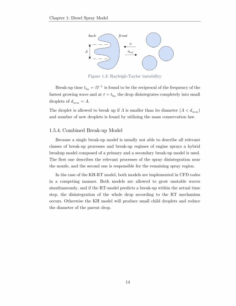
Break-up time 𝑡𝑏𝑢 = 𝛺−1 is found to be the reciprocal of the frequency of the fastest growing wave and at 𝑡 = 𝑡𝑏𝑢 the drop disintegrates completely into small droplets of 𝑑𝑛𝑒𝑤 = 𝛬.
The droplet is allowed to break up if 𝛬 is smaller than its diameter (𝛬 < 𝑑𝑛𝑒𝑤) and number of new droplets is found by utilizing the mass conservation law.
1.5.4. Combined Break-up Model
Because a single break-up model is usually not able to describe all relevant classes of break-up processes and break-up regimes of engine sprays a hybrid breakup model composed of a primary and a secondary break-up model is used. The first one describes the relevant processes of the spray disintegration near the nozzle, and the second one is responsible for the remaining spray region.
In the case of the KH-RT model, both models are implemented in CFD codes in a competing manner. Both models are allowed to grow unstable waves simultaneously, and if the RT-model predicts a break-up within the actual time step, the disintegration of the whole drop according to the RT mechanism occurs. Otherwise the KH model will produce small child droplets and reduce the diameter of the parent drop.
Figure 1.3: Rayleigh-Taylor instability

Chapter 1: Diesel Spray Model
15
Figure 1.4: Catastrophic breakup schematics in KH/RT model
Typically a breakup length is set so only KH stripping breakup occurs in that length . This is due to the fact that reduction of droplet size by the RT model is too fast. After that the KHRT model is fully applied in a competing manner and droplets break up for whichever conditions of KH or RT that applies.
Figure 1.5: Combined blob-KH/RT model
The numerical implementation of these equations as well as the important simulation parametes are examined in more detail in the next chapter.

16
2. OpenFOAM and Lib‐ICE
Chapter2 OpenFOAM and Lib-ICE
CFD enables the possibility of flow study without conducting experiments nor needing to measure flow characteristics at desired locations. It also allows for the study of flow phenomena at a much cheaper cost than experiments, it is non-intrusive and repeatable and it can be utilized to conduct parametric studies faster than experiments. Whether it is flow simulation in micro tubes or biomedical simulations of drug distribution through arteries, CFD has enables us to understand the world in unprecedented ways.
As any physical simulation, CFD results are as good as the embedded physics. Due to highly complex physics behind fluid flow, the CFD implementations are susceptible to simplifications, mistakes or incorrect assumptions and here lies the inherent problems related to CFD simulations and interpretation of its results. This is why experimentation in the world of fluid flow simulations is an invaluable and inseparable asset. In other words, CFD and experiments complement each other and are both utilized in tandem to understand fluid flow phenomena.
Despite the complications with attaining experimental studies of diesel injection [10, 24], there is a rather large pool of experimental data made available through the ECN platform and this experimental data is invaluable in addressing flow simulations and research. In this project, the simulation results were validated using these available experimental results and simulation parameters were fine tuned for more reliable simulation results. It is through these attempts that a better understanding of the diesel DI injection could be attainable and make further enhancement to diesel emissions and energy requirements possible [25, 26].

Chapter 2: OpenFOAM and Lib-ICE
17
In this chapter various techniques used to implement the governing equations in Lib-ICE are outlined and discussed. Further details and description of the OpenFOAM package and the Lib-ICE library can be found in the respective user documentations [27, 28].
2.1. CFD Model
As discussed before, over the years, use of simulations for diesel fuel injection has become common practice. Even though early approaches were limited to predicting some of the principal characteristics of the spray such as penetration values, complex and comprehensive models have been developed [17, 29]. Notable software typically used include commercial software such as Convergent science (Madison, WI), ANSYS (Canonsburg, PA), KIVA (Los Alamos National Laboratory, Los Alamos, NM), AVL (Graz, Austria) and CD-Adapco (now part of Siemens PLM, Plano, TX) [2].
Developed by OpenCFD (an ESI group company), OpenFOAM [30, 31] is a free-to-use Open Source numerical simulation software with extensive CFD and multi-physics capabilities and is released under an open source (GPL) license by the OpenFOAM foundation. With a fully documented source code and no license fees, OpenFOAM has seen steady growth and adoption and provides a collaborative open environment. In this work a CFD solver for spray simulation in direct injection Diesel engines has been implemented in Lib-ICE, an OpenFOAM library for internal combustion engine simulations developed by the ICE group of Politecnico di Milano using the solver named dieselFoamAutoRefine designed for diesel spray modeling.
2.1.1. OpenFOAM setup
Each spray simulation consists of three main parts. First folder called “0” is the initial and boundary conditions setup. This involves parameters such as the initial mass fraction of species (detailed in section 1.3.5) in the combustion chamber, the thermodynamic quantities Pressure, Temperature and Velocity fields and mixture fraction Z.
The second portion of the setup, organized in the folder “constants” involves all the information related to the physical models that will be used by the simulation as well as the geometry. This includes all various parameters needed to implement the desired physics discussed in the previous chapter.

Chapter 2: OpenFOAM and Lib-ICE
18
The third folder named “system” deals with code convergence limits and the main simulation control parameters including time advancement and discretization schemes. Information about how dieselFoamAutoRefine solves the equations are stored in the fvSchemes, fvSolution and controlDict and will be discussed here.
The Lagrangian solver provided by Lib-ICE library uses several phenomenological models including atomization, secondary breakup, collision, drag, evaporation, heat transfer, and turbulent dispersion models to describe processes occurring in the sub-grid length scales. During the injection duration, large and spherical drops (called blobs or parent parcels) are continuously injected to the gas phase [32]. The following section details the interaction between the Eulerian and Lagrangian phases.
2.2. Numerical Schemes
2.2.1. Equation discretization
The system of nonlinear partial differential equations (PDEs) as described in the previous chapter cannot be analytically solved. Discretization schemes are adopted to transform the PDEs into discrete algebraic equations which can be treated numerically. Finite volume method (FVM) is widely adopted in most commercial and open source CFD software and is also adopted in OpenFOAM.
Figure 2.1: Parameters in finite volume discretization
In this method the flow domain is divided into smaller portions which form the computational grid as a whole which is represented in the next sections. Dependent variables and properties are mainly stored in cell centroid P, otherwise they may be stored on faces or vertices. Flow properties are constant within these non-overlapping sub domains and obtained by integrating the

Chapter 2: OpenFOAM and Lib-ICE
19
PDEs over each sub-domain and solving them iteratively. As the number of grid divisions increases, the solution of the discretized equations approaches the exact solution of the corresponding PDEs, since as the control volumes become smaller, difference in variables between neighboring cells become smaller and thus the interpolation become less influential. The schemes adopted are reported in this chapter. Each category of mathematical terms which makes up a PDE can be discretized by several methods which is discussed below.
The Laplacian term is integrated over a control volume. By using the Gauss theorem, the volume integrals are switched into surface integrals and the term is discretized as denoted below.
∫ ∇𝑉
. (𝛤∇𝜙) 𝑑𝑉 = ∫𝑑S𝑉
. (𝛤∇𝜙) = ∑ 𝛤𝑓S𝑓𝑓
. (∇𝜙)𝑓 (2. 1)
The laplacian coefficient 𝛤𝑓 is calculated by interpolating through centeral differencing of centroid values of two neighbouring cels P and N. The face gradient is implicit in case of orthogonal neghbour cells (the normal to the shared face is parallel to the vector d, connecting life of their centroids).
Γ𝑓 = 𝑓𝑥Γ𝑃 + (1 − 𝑓𝑥)Γ𝑁 (2. 2)
S𝑓. (∇𝜙)𝑓 = ∣S𝑓∣ 𝜙𝑁 − 𝜙𝑃|d|
+ 𝑘. (∇𝜙)𝑓 (2. 3)
In case of non-orthogonality, an additional explicit term, k, is used.
𝑓𝑥 = 𝑓𝑁̅̅̅ ̅̅ ̅̅ ̅ /𝑃𝑁̅̅̅ ̅̅ ̅̅ ̅̅ . 𝑓𝑁̅̅̅ ̅̅ ̅̅ ̅ is the distance between face (f) and centroid N and 𝑃𝑁̅̅̅ ̅̅ ̅̅ ̅̅ is the distance between the two centroids.
The convection term is integrated over a control volume by applying the Gauss theorem and linearized as follows
∫∇𝑉
. (𝜌U𝜙) 𝑑𝑉 = ∫𝑑S𝑉
. (𝜌U𝜙) = ∑ Sf𝑓
. (𝜌U)𝑓𝜙𝑓 = ∑𝐹𝜙𝑓𝑓
(2. 4)
𝜙𝑓 is the face field and can be evaluated using a variety of schemes such as the upwind scheme which approximates 𝜙𝑓 by using neighbouring cells based on flow direction. Other shcmes such as central difference interpolation or as mostly used in this simulation, linear interpolation, interpolate 𝜙 based on nearest two cell centroids with a second order accuracy.

Chapter 2: OpenFOAM and Lib-ICE
20
2.2.2. Temporal Discretization
In addition to domain discretization, in case of transient CFD models, an integration over time is also needed.
Time domain is divided into smaller time steps ∆ . For this simulation the implicit time discretization is used with an Euler first order discretization and fixed interval of 2e-07 seconds.
If we denote all the spatial terms as 𝒜𝜙 where 𝒜 is any spatial operator such as the Laplacian, then we can express a transient PDE in integral form as follows:
∫⎣⎢⎡
𝜕𝜕𝑡
∫ 𝜌𝜙 𝑑𝑉𝑉 ⎦
⎥⎤𝑑𝑡 =𝑡+Δ𝑡
𝑡
∫ (𝜌𝑃 𝜙𝑃 𝑉 )𝑛 − (𝜌𝑃 𝜙𝑃 𝑉 )0
Δ𝑡𝑑𝑡 = (𝜌𝑃 𝜙𝑃 𝑉 )𝑛 − (𝜌𝑃 𝜙𝑃 𝑉 )0
Δ𝑡Δ𝑡
𝑡+Δ𝑡
𝑡
(2. 5)
The second term can be expressed as:
∫⎣⎢⎡ ∫𝒜𝜙 𝑑𝑉
𝑉 ⎦⎥⎤ 𝑑𝑡 =
𝑡+Δ𝑡
𝑡
∫ 𝒜∗𝜙 𝑑𝑡𝑡+Δ𝑡
𝑡
(2. 6)
Where 𝒜∗ represents the spatial discretization of 𝒜. For the Eulerian method adopted in this work the first order accurate scheme is as follows:
∫ 𝒜∗𝜙 𝑑𝑡𝑡+Δ𝑡
𝑡
= 𝒜∗𝜙0 𝑑𝑡 (2. 7)
𝜙0 refers to the old values of spatial terms.
This method’s stability is not ensured and in order to have stability the time step cannot be larger than a maximum value, which depends on the Courant number
𝐶𝑜 = 𝑢∆𝑥∆𝑡
(2. 8)
Where is the magnitude of the velocity and ∆ is the grid sizing. To ensure stability, courant number needs to be below one. In this simulation a maximum
value of 0.25 was used.

Chapter 2: OpenFOAM and Lib-ICE
21
2.2.3. Summary
The following is a summary of the numerical schemes used in this simulation.
Table 2.1: Numerical schemes for the divergence terms used
default Gauss limitedLinear 1.0
div(phi,U) Gauss limitedUpwind grad(U)
Table 2.2: Numerical schemes for the other terms used
ddtSchemes Euler
laplacianSchemes Gauss linear corrected
gradSchemes Gauss linear
interpolationSchemes linear
snGradSchemes corrected
2.3. Eulerian-Lagrangian Coupling
As discussed in the previous chapter, the spray is described in a Lagrangian fashion by a number of parcels injected into the domain where each parcel is representative of droplets with the same properties. The gas medium however, is treated in an Eulerian fashion and the spray evolves into the domain based on the mass, momentum and energy exchange with the continuous gas phase.
The Eulerian and Lagrangian phases interact with each other in order to determine the mixture formation and the evolving spray. The phase coupling can be distinguished into tow part of gas-liquid and liquid-gas [11].
2.3.1. Gas-Liquid Coupling
Gas-liquid coupling includes the interpolation process so that the gas properties known at the Eulerian nodes are estimated at the location of the parcels.
At first the velocity field which is known at the cell centers is evaluated at the closet vertices or faces. Then, a tetrahedron is built with the closest points around each parcel.

Chapter 2: OpenFOAM and Lib-ICE
22
i
i
Vertex i
Base i
x
Figure 2.2: Parcel position interpolation
The distance between the parcel and one of the tetrahedron faces is , while represents the distance between the same face and its opposite vertex.
The interpolated velocity at the parcel position x is:
𝑢(𝑥) = ∑ 𝛽𝑖𝛼𝑖 + 𝛽𝑖
𝑢𝑖
4
𝑖=1(2. 9)
This method ensures that the parcels experience a continuous velocity field. And the momentum exchage after obtaining the velocity field at parcel location is calculated according to the eqautions explained in section 1.4.
2.3.2. Liquid-Gas Coupling
The liquid-gas coupling is the effect of spray source terms on the Eulerian governing equations.
The Eulerian solution is frozen at time instant and the parcels are advanced one by one to the next time step of 𝑛 + 1. All the source terms in the mass, momentum and energy equation are thus evaluated at the time 𝑛. Each parcel is tracked along its path by using the face-to-face algorithm. This makes possible to identify all the cells crossed by each parcel during one time step and to split the Lagrangian source terms of the Eulerian equations accordingly. If the velocity of the parcel is lower than the interpolated Eulerian velocity it will gain momentum which is taken from the Eulerian phase and reduce the Eulerian velocity. The droplet temperature, however, is not obtained by means of interpolation on the Eulerian phase. Instead, the energy equation accounts for heat transfer and evaporation of the droplets. The time advancement mechanism is discussed in more detail in this chapter.

Chapter 2: OpenFOAM and Lib-ICE
23
Every parcel is injected from a point located in a disk whose size is equal to the injector nozzle and the points are randomly chosen according to a uniform distribution. The frequency of the addition of new parcels is directly related to the fuel injection rate (ROI), assuming constant density of the liquid fuel and ideally spherical droplets. Following the blob injector model (1.5.1), every injected parcel is characterized by the same diameter which is comparable to the size of the nozzle hole on the gas side.
𝑁(𝑡) = 𝑚𝑎𝑥 (1, 𝛥𝑡 𝑁𝑡𝑜𝑡𝑡𝑒𝑜𝑖 − 𝑡𝑠𝑜𝑖
) (2. 10)
is the total number of parcels. There was an attempt to increase the total number of injected Parcels to around 100,000 but due to instabilities in the runtime this number was reduced to 30000. and indicate the time of end and start of injection respectively.
2.4. Pressure and Velocity Coupling
Since an explicit equation for the pressure in the Navier-Stokes equations is not available, a coupling scheme relates the pressure values to the velocity field. The algorithm used in this project is a PIMPLE algorithm which is a coupling of SIMPLE and PISO algorithms [27]. This algorithm utilizes an inner PISO loop with the addition of an outer correction loop which includes cycling over the same time step using the previous iteration result as initial guess for next iteration. It should be noted that the non-orthogonality of typical chamber meshes requires higher correction loops and the PIMPLE algorithm shows its strength by enabling the use of larger time steps. In this specific simulation, however, the structured grid and relatively lower cell size reduces the significance of this method.
2.5. Computational Grid
A collection of experimental geometry measurements for Spray A has led to the generation of educated 3D surface files, smoothed to remove experimental artifacts and provided through ECN. However, in the simulations conducted for this report, the focus was on a simplified wedge type mesh which was created in OpenFOAM using the blockMesh method. The 3D mesh file was only used for calculations of geometric ratios of the injector and cross checking with similar studies on Spray A. The wedge type domain is schematically presented

Chapter 2: OpenFOAM and Lib-ICE
24
in the following figure where a small slice of the cylinder with an angle less than 5 degrees is considered:
Figure 2.3: Schematics of the Wedge type domain
Thus the main focus would be on the 2-D plane with the axisymmetric edge on the left and the cylinder walls on the other edges where the injector is positioned at the top right as presented the following scheme. In the wedge type domain no divisions are applied in the y-direction; this is how OpenFOAM interprets the 2D solver and will ignore that dimension.
Figure 2.4: 3D schematic of the Wedge type geometry
The mesh is discussed in more detail in the next chapter.
2.6. Performance Indexes
This section denotes the main spray measurements of interest used to evaluate the simulation results and comparison with the empirical data.
Chapter 2: OpenFOAM and Lib-ICE
25
2.6.1. Liquid Length
This value denotes the maximum extent of liquid-phase spray penetration during injection. It is measured using methods such as diffused back-illumination extinction (DBI) method, Phase Doppler Particle Analyzer (PDPA), Mie scattering, laser-induced fluorescence (LIF) [8, 21, 26, 33].
The process of atomization of sprays is responsible of creating thousands of droplets with different diameters. For example in the case of DBI method, the droplets result in a laser intensity loss respect to the initial light intensity due to scattering. The optical depth (or optical thickness ) is basically the fraction of light that passes across such a turbid medium which has not been absorbed or scattered.
In Lib-ICE, the liquid length evolution as function of time is stored in a file named sp99.Bomb. It is defined as the axial distance from the injector where 99% of the liquid mass was found, which is the definition which is mostly used for comparison with experimental data of liquid spray penetration.
The steady state liquid length was defined as the average of the sp99 values from 0.45 ms to 1.2 ms. This threshold was observed to be well after the initial ramp up and able to filter out all the inherent noise in the values of sp99.
2.6.2. Jet Penetration
Shadowgraph or Schlieren imaging are used to identify the vapor boundary of a penetrating jet [34]. The boundary of the spray is determined through image analysis and the penetration distance is defined as the distance along the spray axis to the boundary of the spray. In the OpenFOAM library the fuel vapor penetration evolution as function of time is stored in a file named vapPen1.Bomb. It is defined as the maximum axial distance where a mixture fraction value of 1e-3 was found. This is the definition which is currently used for comparison with experimental data of fuel vapor penetration.
In this work, the liquid and vapor penetration values are reported in a same figure with the following schematics.

Chapter 2: OpenFOAM and Lib-ICE
26
Time [ms]
Pene
trat
ion
Len
gth
[m]
Liquid Penetration sp99
Vapor Penetration vapPen1
Figure 2.5: Schematics of the penetration values over time
2.6.3. Spray Mixing Line
The evaporation of diesel spray has a direct effect on the combustion rate since only vaporized fuel that has been mixed with air in a combustible ratio can chemically react with the oxygen contained in the fresh air intake.
The idea behind the mixing line is to assess whether the spray evaporation is mixing limited. Existing phenomenological spray models are roughly distinguished into two modeling schools, namely the droplet limited evaporation and the mixing limited evaporation. In the droplet limited case, the droplet evaporation process is the limiting factor for spray formation whereas in the mixing limited models the vaporization rate of the fuel is limited by the mixing rate of fuel and ambient gas. The vapor-liquid thermodynamic equilibrium is assumed to settle immediately, which makes the amount of air entrained a direct limiting factor [35].
The enthalpy balance for the mixture is expressed in terms of an adiabatic mixing process [36]:
ℎ(𝑇 ) = 𝑍. ℎ𝑓(𝑇0) + (1 − 𝑍). ℎ𝑎(𝑇𝑎) (2. 11)
ℎ𝑓(𝑇0) is the enthalpy of fuel at the fuel temperature and ℎ𝑎(𝑇𝑎) is the enthalpy of air at the ambient temperature. Following this equation, the spray mixing line is expected to resemble Figure 2.6.

Chapter 2: OpenFOAM and Lib-ICE
27
Z [%]T
[K]
Figure 2.6: schematic of an ideal mixing limited spray mixing line
In order to investigate and ensure that the spray simulation is of the mixing limited evaporation nature, the mixture fraction at the location of the injected parcels is compared to the local temperature in the vicinity of the parcel. If the spray simulation is mixing limited then the lower mixture fractions should be the result of more fuel evaporation and in turn, temperatures closer to ambient temperature is expected. However, other effects such as heat transfer close to the nozzle tip could affect the mixture fraction and cause a scatter and dispersion in the spray mixing line as denoted in Figure 2.7.
Z [%]
T[K
]
Figure 2.7: Schematics of the dispersion of the spray mixing line
The wider the dispersion visible in the mixing line, the more likely it is that the evaporation is not mixing limited and some other factor has influenced the evaporation process and thus the simulation results might show significant deviation from the experimental data.

Chapter 2: OpenFOAM and Lib-ICE
28
2.6.4. Spray Shape
Fuel is injected by means of the injector fed by the common rail. Typically there is a certain coefficient associated with the nozzle of the injector where the geometrical features of the needle coupled with the amount of inflicted pressure difference will reduce the actual injection area to an effective amount due to cavitation. The spray covers a 3D conical shape and starts in the optically thick region where the primary breakup schemes occur followed by the secondary breakup. The spray will eventually evolve into the optically thin regions where the injected liquid is essentially evaporated and the steady state penetration length of the spray can be seen.
Figure 2.8: Schematics of the diesel spray
In the dieselFoamAutoRefine solver, the Lagrangian approach provides a method of visualization to understand the spray cone as well as the diameter of the liquid droplets at any parcel location. This method was utilized in conjunction with the mean void fraction of the domain which represents the volume fraction occupied by the gas phase in and the result was helpful in a better visualization of the simulated spray.
Another benefit of this approach is the possibility to distinguish the gradual reduction of liquid droplets as the spray evolves into the domain and study the

Chapter 2: OpenFOAM and Lib-ICE
29
effect of various breakup model parameters on spray evaporation. The results are presented in the next chapter.
Cavitation is schematically represented in the figure above. It is noteworthy that the injector shape has a great deal of influence over cavitation. For example smooth guiding injector walls allows for the streamlines to better follow the injector contours and prohibit cavitation.
2.7. Simulation Parameters
Apart from the adjustment of turbulence model coefficient 𝐶1, some of the influential simulation parameters include KH-RT model parameters as well as the L/D ratio of the injector which has impact on the blob model. They have a definitive impact on the performance indexes discussed in the previous section and require a careful calibration for the spray simulations.
The following is a summary of these variables and a short description.
B0: this constant must be fixed to 0.61. It regulates the size of stripped secondary droplets according to the KH breakup mechanism. In the fourth ECN workshop the B0 value, typically considered constant, has been subject to study and modifications. Nonetheless it is mainly a fixed constant.
B1: tuning constant for Wave breakup. It controls the diameter reduction of
secondary droplets, according to breakup length and timescales. Lower 𝐵1 results in higher diameter reduction rate.
Ctau: constant of the RT breakup model.
CRT: constant that regulates the size of the most unstable RT breakup waves. Range: 0.05 - 2. The smaller it is, the earlier catastrophic breakup will take place.
WeberLimit: below this value, secondary droplets do not experience breakup. Droplet disintegration is greatly influenced by the Webber number [37].
msLimit: parameter to control the generation of new droplets originating from wave breakup.
cBU: coefficient regulating the breakup length. The higher it is, the farther from nozzle RT breakup will take place as represented in Figure 1.5.

Chapter 2: OpenFOAM and Lib-ICE
30
2.8. Post Processing
In a CFD simulation, post processing includes all the activities needed to make sense of the raw data and make them useful in order to be able to draw conclusions. In this work, the open source software named Paraview [38] was utilized for flow visualizations as described in section 2.6.4. In the next section the methods used to access Paraview and generate automated figures for each simulation case is described in brief.
2.8.1. Automation Scripts
Case tuning and making sense of the data required a sizable database of simulation results for various setup parameters. This was rendered possible through the use of the powerful computers indispensable to the department of energy of Politecnico di Milano. Remote access through the Secure Shell (SSH) limited the data accessibility and the double checking of the setup and this resulted in some poor case setup and unusable simulation results and wasted CPU time on the nodes. In order to prevent these shortcomings a series of python modules was developed and utilized in a Python script. This automation enabled case setup with the desired values in bulk and with high confidence in the case setup and made room for more focused data analysis free from doubts about the correctness of the case setup.
A number of important simulation parameters were defined in a script and the subsequent particular folder structure was made ready for OpenFOAM to utilize. Coupled with easy simulation initiation commands, real-time monitoring of the remote simulation and archiving schemes; this method was very effective in removing as many areas of probable missteps and friction as possible.
In addition to simulation automation scripts, the need for some form of automation in the area of post processing was felt. Additional Python scripts utilizing Paraview.simple [39] modules was developed which would produce relevant charts and figures related to the region near the nozzle. Including a particle Lagrangian field, a mixture fraction field and the spray line delineating the mixture fraction versus cell temperature.
Additional scripts using LaTeX, turned the produced figures into a single PDF page already containing simulation parameters and relevant numbers.
The result was a sizable database of simulations covering a rather wide range of parameters (detailed in section 2.7). This was quite helpful in case tuning

Chapter 2: OpenFOAM and Lib-ICE
31
and matching of the simulation results to experimental results which were available through multiple institutions and other studies. Visualization of the simulation results facilitated data analysis and trend observation necessary in performing a useful and reliable CFD simulation.
Despite available suggestion for the range on many of the spray simulation parameters, these visualizations lead to a form of sensitivity analysis so while staying in the suggested ranges, the final simulation was based on the setup that had the best agreement with available data.
Multiple experimentations have already been carried out related to the ECN workshop and producing spray mixing simulations. These experiments are valuable in spray studies and useful in predictions or parametrizations of certain aspects of the mixing phenomenon. Successful CFD simulation of spray mixing and evaporation needs a careful study of available data so the final simulation result are in best agreement with available experiments.

32
3. Model Validation
Chapter 3 Model Validation
As discussed previously, the importance of experimental results cannot be overstated in CFD model validation and this is even more emphasized in case of diesel injection simulation due to existence of various models utilized in describing the flow phenomena and breakup regime. In this chapter the details of the ECN sprays are discussed.
3.1. Spray case study
The ECN working group has identified a few experimental conditions that will be the focus of modelers and experimentalists who wish to voluntarily participate in the ECN in the future. The experimental collaboration is made possible by the donation of identical injection systems by Robert Bosch LLC. The ECN group has agreed to experiment at the same injector and ambient conditions, thereby leveraging the expertise of each participant, and enabling direct comparison between different facilities. The expectation is that the data set developed will become a serious focal point for model validation and further advanced diagnostics.
There are various Sprays that are the main focus of the ECN workshops: Spray A, B, C and D. Each with a unique injector, number of injection holes and diameter. Each spray has been subject to a number of experimental tests and the history of location and use of each one is documented and maintained. There are also variations within each Spray specified with the injector serial number. These variations are important as there would be minor differences in the nuanced geometry of each injector and thus the research would be focused on one specific serial number of a spray in order to minimize the potential differences in experiments or simulations.

33
3.1.1. SNL Experimental Setup
The main experiment of interest in this study is conducted by Sandia National Laboratories. The experiment is conducted in a vessel which is constant volume and optically accessible capable of withstanding high pressure and temperature levels.
Figure 3.1: Optically accessible constant volume SNL spray chamber
The chamber is a Cross-Optical, Cube-Shaped Vessel with the following schematics:
Figure 3.2: The SNL vessel shcematic
Figure 3.2 shows a schematic cross-section of the combustion vessel. The vessel has a cubical-shaped combustion chamber. With full optical access, the following ambient conditions can be generated:

Chapter 3: Model Validation
34
• Ambient gas temperatures from 450 to 1300
• Ambient gas densities from 3 to 60 /
• Ambient gas oxygen concentrations from 0% to 21%
These conditions span or exceed those typically experienced in a diesel engine.
Fuel is injected using common-rail fuel injectors. The characteristic dimension of the cube is 108 mm. Each side of the combustion chamber has a round port with a diameter of 105 mm. The fuel injector is located in one side port using a metal insert that forms the right wall of the combustion chamber. Two spark plugs and a mixing fan are mounted in another metal insert that forms the top wall of the chamber. Optical access is provided by four sapphire windows with clear apertures of 102 mm located in the other four ports. For wall heat transfer modeling purposes, the steel vessel and metal inserts for the injector and spark plugs are made of 4340 steel.
Figure 3.3: The Combustion Chamber
A picture of the inside of the combustion vessel is shown in Figure 3.3. Visible objects include the spark plugs, mixing fan, injector, intake valves, and a beaded thermocouple. Two spark plugs are used to produce consistent combustion in the high-density, fuel-lean environment. The spark gap located is 16.5 mm below the vessel top and at a radius of 31.8 mm relative to center of vessel. Electrode diameter is 3.2 mm. Ground strap diameter is 1.6 mm. Ground strap leads (in-line with the electrode) are separated by 21 mm.

Chapter 3: Model Validation
35
The mixing fan at the center is operated at 8000 rpm to ensure uniform ambient conditions at the time of injection. The bottom of the fan is approximately 15 mm below the top. The outer diameter of the fan is 25 mm. There are eight fan blades, oriented at a 30 degree angle relative to horizontal, attached to a 7 mm disk at the center. Fan blades are 0.85 mm thick.
Figure 3.4: Chamber Volume Schamatics
Intake and exhaust valves, or instruments such as pressure transducers or thermocouple inputs, are mounted at the corners of the cubical-shaped combustion chamber. Figure 3.3 and the solid model of the chamber volume presented in Figure 3.4, show that the edge of the cube is an extension of the 105 mm cylindrical ports with a 19.05 mm port hole going exactly through the corner of the cube. Closed valves are recessed a depth of 4 mm from the highest part of the extended cylinder ports. Note that the windows are recessed some from the 105 mm bored port diameter, so that the effective cube dimension is 108 mm. The injector protrudes into the vessel consequently affecting the vessel geometry.

Chapter 3: Model Validation
36
Figure 3.5: Half and full 3D chamber view
3.1.2. Spray Characteristics
The ECN group has agreed to experiment at the same injector and ambient conditions but recommendations for parametric variation beyond Spray A are also available. The Spray A condition is a low-temperature combustion condition relevant to engines that use moderate EGR. The injector specifications are for modern advanced injection systems with high pressure capability. As a prerequisite to using these injectors, ECN participants are expected to measure the boundary conditions (e.g. temperature, pressure) for the ambient and injector quantities, and uncertainties associated with the boundary conditions and other data.
The so called standard condition is concerned with the Spray A and a specific set of conditions and detailed below [40].
Table 3.1: Spray A specifications and operating conditions
Ambient gas temperature 900 K
Ambient gas pressurea near 6.0 MPa
Ambient gas densitya 22.8 kg/m3
Ambient gas oxygen (by volume)
15% O2 (reacting); 0% O2 (non-reacting).
Ambient gas velocity Near-quiescent, less than 1 m/s
Common rail fuel injector Bosch solenoid-activated, generation 2.4
Fuel injector nominal nozzle outlet diameter
0.090 mm
Nozzle K factor K = (𝑑𝑖𝑛𝑙𝑒𝑡 − 𝑑𝑜𝑢𝑡𝑙𝑒𝑡)/10 [use 𝜇𝑚] = 1.5

Chapter 3: Model Validation
37
Nozzle shaping Hydro-eroded / Smoothed by hydro-erosion
Mini-sac volume 0.2 mm3
Discharge coefficient at 10 MPa pressure drop 𝐶𝑑 = 0.86 (room temperature, diesel fuel)
Number of holes 1 (single hole)
Orifice orientation Axial (0° full included angle)
Fuel injection pressure 150 MPa (1500 bar), prior to start of injection
Fuel n-dodecaneb
Fuel temperature at nozzlec 363 K (90°C)
Common raild GM Part number 97303659. Used by 2005-2006 Duramax engines.
Common rail volume/length 22 cm^3/28 cm
Distance from injector inlet to common rail
24 cm
Tubing inside and outside diameters
Inside: 2.4 mm. Outside: 6-6.4 mm.
Fuel pressure measurement 7 cm from injector inlet / 24 cm from nozzle
Injection duration 1.5 ms
Injection mass 3.5 - 3.7 mg
Approximate injector driver current
18 A for 0.45 ms ramp, 12 A for 0.345 ms hold
a) This exact combination of ambient pressure and density corresponds to a particular set of gases for a 0% O2 condition with 89.71% N2, 6.52% CO2, and
3.77% H2O by volume and a compressibility factor, Z =1.01. When different gases are used, the pressure must vary to maintain the same density.
b) Chosen as a fluorescence-free diagnostics fuel with known chemistry and properties. Other fuels may be selected after initial study and comparison.
c) May be slightly different than injector body temperature. d) Use rail outlet farthest away from fuel entrance (small orifice) to rail.
Well defined parametric variation about the Spray A conditions is useful for more deliberate model validation and cross checking between experimental facilities. This report will not go into the detail of experimentations but the

Chapter 3: Model Validation
38
results of the experiments conducted by various institutes covering a wide range of operating conditions and parameters are available. Experimental conditions such as ambient temperature, ambient density, injection pressure, nozzle size, fuel type, etc. were varied for a given experimental diagnostic. As there are many different combinations of variables, a search utility has been developed to quickly display the data of interest.
3.1.3. Rate of Injection
Injection rate profiles, and the discharge and area-contraction coefficients were measured by injecting onto a force transducer and simultaneously collecting and weighing injected fuel [34, 41]. In this section some aspects of the injector and the experimental method are discussed in brief.
As the development of a spray is dependent on both the mass and momentum flow rates from an orifice, two orifice coefficients are used to characterize these flow rates.
𝐶𝑑 = 𝐶𝑎𝐶𝑣 (3. 1)
Using 𝐶𝑣 and 𝐶𝑎, the mass flow rate �̇�𝑓 and momentum flow rate �̇�𝑓 from an orifice are given by the following:
𝑚�̇� = 𝐶𝑎.𝐴𝑓. 𝜌𝑓 . 𝐶𝑣. 𝑈𝑏 (3. 2)
𝑀�̇� = �̇�.𝐶𝑣.𝑈𝑏 (3. 3)
Where 𝑈𝑏 is given by the Bernoulli’s equation:
(𝑃 + 12
𝜌𝑈2 + 𝜌𝑔ℎ)𝑃𝑟𝑖𝑜𝑟 𝑡𝑜 𝑂𝑟𝑖𝑓𝑖𝑐𝑒
= (𝑃 + 12
𝜌𝑈2 + 𝜌𝑔ℎ)𝐴𝑓𝑡𝑒𝑟 𝑡ℎ𝑒 𝑂𝑟𝑖𝑓𝑖𝑐𝑒
(3. 4)
𝑈𝑖𝑛𝑗,𝑚𝑎𝑥 = √2.[𝑃𝑓 − 𝑃𝑎]
𝜌𝑓(3. 5)
The velocity 𝑈𝑖𝑛𝑗,𝑚𝑎𝑥 is the maximum potential fluid velocity at the orifice exit, while the product 𝐶𝑣 · 𝑈𝑏 is the average velocity at the orifice exit over the area 𝐶𝑎 · 𝐴𝑓 .
The orifice area-contraction coefficients were determined from the spray momentum measured with a force transducer and the following relationship derived from previous equations.

Chapter 3: Model Validation
39
𝐶𝑎 = 2.𝐴𝑓. 𝐶𝑑2.
(𝑃𝑓 − 𝑃𝑎)�̇�𝑓
(3. 6)
�̇�𝑓 Mass flow rate
�̇�𝑓 Momentum flow rate 𝑈𝑏 Velocity of the stream right after the orifice 𝐴𝑓 Orifice exit area 𝜌𝑓 and 𝜌𝑎 Fuel density and ambient density 𝑃𝑓 and 𝑃𝑎 Fuel pressure and ambient pressure The injection rate profiles show that the opening and closing of the injector occurs in less than 0.1 ms. Injection is nearly steady during the time of injection, creating a square-wave injection rate shape [34]. As opening and closing times are small, the average momentum (𝑀𝑓) during the steady-flow period was used to determine the orifice coefficients.
As for the numerical simulation, ROI is determined based on the results of the experimental campaign performed to a pool of standard ECN injectors and evaluates the impact of the nozzle geometry on the hydraulic performance and cavitation phenomenon [42]. The study investigates the effects of geometry, back pressure, injection pressure, etc. on the Injection rate. It is shown that in general, very similar mass flow rate and momentum flux rate curves are obtained in each group of injectors (Spray C and Spray D). During the steady state period, the ROI results seem to scale with the actual outlet diameters with certain non-dimensional scaling factors.
To generate the ROI of a particular nozzle orifice, the nominal mass flow of the corresponding nozzle orifice which is provided by measurements, must be multiplied by the normalized non-dimensional shape of ROI [42]. These numbers were tabulated and the corresponding ROI was calculated. A trapezoidal numerical integration was used to calculate the total injected mass needed by OpenFOAM. The injection duration was set to be 1.5 ms denoted by “SHORT”. As opposed to 4.5 ms “LONG” injection duration which was not considered in this report.

Chapter 3: Model Validation
40
Figure 3.6: ROI for Spray C with Injection Pressure of 50MPa
The figure above is an example of ROI profile for spray C where rail injection pressure is 50MPa and the ambient back pressure is 2MPa. In this case the non-dimensional mass flow rate multiplier is 1.9104. The final rate of injection profile is added to Lib-ICE using the injectorProperties file which involved the detailed injection rate, total mass to be injected and the 𝐶𝑑 value.
3.1.4. Target Sprays
The target injector for Spray A modeling efforts was selected to be the injector with the serial number of 210675 which is simply referred to as “675”. Spray A has been the subject of exhaustive geometrical measurements [43]. The following table shows the geometric details of this specific injector as opposed to others:
Table 3.2: Geometric details of Spray A
Serial # 𝑫𝒊𝒏𝒋 [mm] Fuel
𝑷𝒊𝒏𝒋 [MPa] 𝑻𝒇𝒖𝒆𝒍 [K]
𝝆𝒇𝒖𝒆𝒍 [kg/m3] 𝑪𝒅 𝑪𝒂
210370 0.0908 n-dodecane 150 343 713 0.89 0.98
210675 0.0894 n-dodecane 150 343 713 0.90 0.98
210677 0.0837 n-dodecane 150 343 713 0.89 0.98
210678 0.0886 n-dodecane 150 343 713 0.89 0.98
0
0.5
1
1.5
2
2.5
0 1 2 3 4 5
Mass flow rate [g/s]
time [ms]
Rate of Injection Profile
Actual mass flow rate Non‐dimensioanl mass flow rate

Chapter 3: Model Validation
41
210679 0.0841 n-dodecane 150 343 713 0.91 0.98
For Spray C, the Spray C210037 was chosen with a nominal nozzle diameter of 0.208 mm. For Spray D, the Spray D209134 was chosen with a nominal nozzle diameter of 0.186 mm. Spray C has a sharper edge for the injector inlet and thus, cavitation is expected in the nozzle and this will reduce the effective nozzle outlet and influence the breakup of the spray as well. Spray D, however, has a smoother surface as presented in Figure 3.7 and less likely to cause cavitation.
Figure 3.7: X-ray tomography of nozzle D (left) and C (right)
3.2. Target Conditions
Considering a fixed ambient density, it is required to adjust the ambient Pressure and Temperature according to the thermodynamic gas law. Thus there is a proportional change in pressure so that the product of pressure and temperature remains constant. The following conditions and sprays were of interest to the fifth ECN workshop and thus the focus was put on them. It is noteworthy that the majority of the attention was in case tuning of Spray A and the other spray simulations were performed with the same simulation constants except for adjustments in Length to Diameter ratio of injectors related to the blob injector model and the suitable rate of injections according to the injector. They were all simulated in the short injection period of 1.5 ms.

Chapter 3: Model Validation
42
Table 3.3: Spray conditions simulated for ECN5
Spray T [K]
A675 700, 800, 900, 1000, 1100, 1200
C003 and C037 850, 900, 1000, 1100
D134 and D135 850, 900, 1000, 1100
3.3. Experimental Parameters
There are a number of parameters carefully studied and reported with regards to each ECN experimental record. A number of these parameters are the so called “Nominal Parameters” which outline the most important setup parameters for a specific spray. The following is a short description of these values.
Nominal Ambient Oxygen Concentration [%],
Defines the mole fraction of ambient oxygen in the vessel. Used for simulating the use of EGR or creating an inert (0% O2) environment. In this case the inert condition was used i.e. 0% O2.
Nominal Ambient Temperature [K],
Gas temperature of the core region of the vessel. The small fan in the combustion chamber keeps this value uniform within the chamber volume.
Nominal Ambient Density [kg/m3],
Gas density of the core region of the vessel. This value is kept constant in this project. Thus upon examining the effects of ambient temperature, the ambient pressure needs to be adjusted according to the ideal gas law. Ambient density value of 22.4kg/m was maintained.
Nozzle Size or Orifice Diameter [mm],
Smallest diameter of injector nozzle. Obtained using Optical microscopy, x-ray tomography, and x-ray phase contrast derived data.
Nominal Injection Pressure Difference [MPa],
Difference between fuel injector pressure and ambient gas pressure.

Chapter 3: Model Validation
43
Nominal Injection Duration
The injection duration was set to be 1.5 ms denoted by “SHORT”. In the datasets the Time After Start of Injection (ASOI) is set as a reference of time keys after which the data such as Liquid Penetration is measured and recorded.
Fuel Type
Only fuel type used for Spray A experiments and simulations is normal dodecane (nC12). Although n-dodecane is not an ideal surrogate for transportation fuels, its choice due to the fact that unlike pump fuels, normal dodecane has been subject to different optical measurements and the physical and chemical properties of the fuel are precisely defined [25]. Another advantage of using normal dodecane is low amounts of soot which helps with experimental setups. Fuel properties are listed below:
Table 3.4: n-dodecane Properties
T100 [°C] 216
Cetane Number 87
Low. Heat. Value [MJ/kg] 44.17
Density at 15°C [kg/m3] 752.1
Aromatics Vol. % 0
H2 mass % 15.3
Sulfur [ppm] 0
Kin. Visc. (-20°C) [mm2/s] 4.7
Kin. Visc. (40°C) [mm2/s] 1.5
Freeze Point [°C] -10
Flash Point [°C] 83
The above mentioned parameters along with the fuel temperature, are the nominal values. Coupled with other information such as the name of the institute or further documentations they are the basis for various spray distinguishing. Other parameters such as the spray shape, liquid length and jet penetration (vapor penetration) as among the important measurements as discussed in section 2.6.

Chapter 3: Model Validation
44
3.4. Grid Convergence
The optimal grid sizing configurations were defined based on two principals: Mesh size and Mesh grading. Three options were chosen for each of these two parameters and the grading was set so the mesh would be much finer closer to the spray region where finer mesh resolution might be needed to capture the flow phenomena properly. This is both due to the injection causing great gradients near the nozzle region as well as the Lagrangian field of parcels being injected in the flow. Simple grading method used is based on the proportion of the first and last divisions along an edge and shown in Figure 3.8:
Figure 3.8: Mesh simple grading along a block edge
Figure 3.9: Finer mesh closer to the Spray
A set of initial simulations clarified the proper grid size. As it will be discussed shortly, there are multiple simulation parameters with a recommended range for spray simulations but the fine tuning of these parameters is a meticulous and time consuming task. Here, the main concern is the grid convergence so we can ensure the simulation results are grid independent and reliable with respect to sizing of the mesh. Coarser mesh will not be able to capture the flow phenomena especially closer to the spray region and an extremely fine mesh will simply put too much computational load on the simulation and render it unviable. The grid convergence study outlined the advantages of the mid to high mesh resolution over the coarse size. Spatial divisions are represented in the following figure showing more refined mesh near the nozzle outlet in case of mesh (c) as opposed to the same number of cells in case of mesh (a) with a less pronounced grading scheme.

Chapter 3: Model Validation
45
a b c
Figure 3.10: Simple grading scheme near the nozzle outlet
Figure 3.11 and Figure 3.12 show the simulation of the spray A and the evolution of liquid and vapor penetration values over time under standard condition. The number of cells was increased and the effect of mesh resolution can be observed.
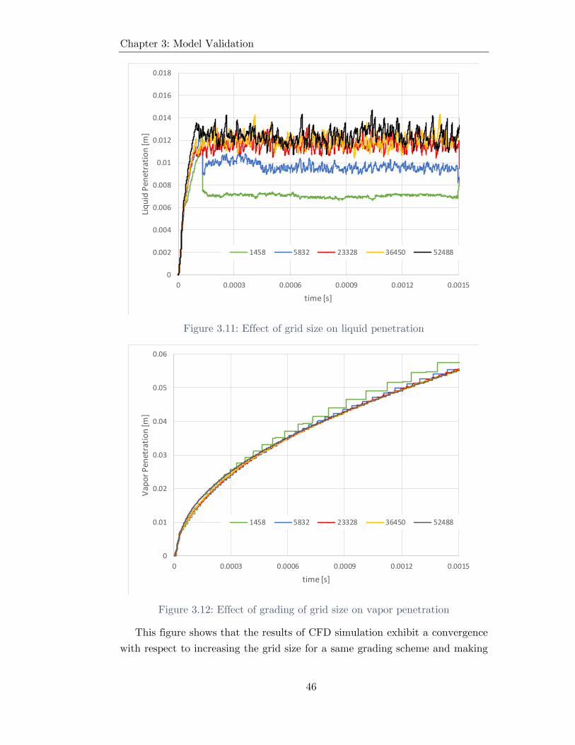
Chapter 3: Model Validation
46
Figure 3.11: Effect of grid size on liquid penetration
Figure 3.12: Effect of grading of grid size on vapor penetration
This figure shows that the results of CFD simulation exhibit a convergence with respect to increasing the grid size for a same grading scheme and making
0
0.002
0.004
0.006
0.008
0.01
0.012
0.014
0.016
0.018
0 0.0003 0.0006 0.0009 0.0012 0.0015
Liquid Pen
etration [m
]
time [s]
1458 5832 23328 36450 52488
0
0.01
0.02
0.03
0.04
0.05
0.06
0 0.0003 0.0006 0.0009 0.0012 0.0015
Vap
or Pen
etration [m
]
time [s]
1458 5832 23328 36450 52488

Chapter 3: Model Validation
47
the grid even finer will not be beneficial in terms of achieving better results and will simply bring about too much computational cost.
It is observed that the smaller grid size results in higher liquid penetration (sp99) and slightly lower vapor penetration (vapPen1). This can be explained due to intricacies of Eulerian-Lagrangian approach adopted in the spray simulation. Three important effects of mesh dependency can be identified [9]:
Calculation of representative gas phase flow quantities at the exact location of the droplets
Distribution of mass, momentum, and energy to the nodes of gas phase Unrealistically fast diffusion due to immediate averaging of the source
terms over the whole cell volume
Finer grid size results in more accurate approximations of differentials and the strong spatial gradients of flow quantities are resolved better. But the implemented Lagrangian methodology calls for proper capturing of the parcels or droplets within the grid and calculating the momentum transfer between the parcel and the engulfing grid cell in a proper fashion so that this exchange is not averaged over a large area and result in unrealistically fast diffusions. So it is expected to obtain more realistic results upon utilizing finer mesh resolutions. In this case the enhanced momentum transfer for finer mesh resolutions results in higher steady state liquid penetration and slightly lower vapor penetration.
Due to diminishing returns upon increasing the number of cells and also due to being able to capture the liquid length in agreement with experimental results the suitable grid size for the simulations was identified. The radial distribution of the mixture fraction at 30 mm axial distance from the injector was also examined for various grid sizing which also helped define the proper grid sizing.

Chapter 3: Model Validation
48
Figure 3.13: Effect of grid sizing on liquid length
The figure above, shows the liquid length grid convergence study. The significant observation is the small change of the steady state liquid length for much higher number of cells. The proper grid size is indicated with a cross. It provides a sizing of 0.127 mm for the smallest division.
Another grid convergence measure was the mixture fraction at 30 mm axial distance from the injector. Figure 3.14 shows the increased accuracy of capturing this curve for more resolute grid sizing. It is observed that the simulation results for the specified sizing is well within an acceptable threshold and the increased number of cells closer to the axisymmetric edge improves the distribution curve details significantly. The curve appears to be well captured and this is even more pronounced for when the data is interpolated to produce a smooth curve where the difference between the fine grid resolutions are not easily distinguishable any more. It should also be noted that the grading scheme increases the number of division at the region closer to the axisymmetric edge. This effect improves the simulation results and helps keep the cell count to a lower value.
0
0.002
0.004
0.006
0.008
0.01
0.012
0.014
0 10000 20000 30000 40000 50000 60000
Steady State Liquid Len
gth [m
]
Number of Cells

Chapter 3: Model Validation
49
Figure 3.14: Effect of grid sizing on mixture fraction at 30 mm
Some other noteworthy aspects of the mesh is the usual quality controls including aspect ratio, skewness, non-orthogonality and cell volume ratio. They all check out well within the suitable range as a structured wedge type mesh was utilized. The aspect ratio of the wedge type mesh used which is the ratio between the biggest and the smallest areas of the cell's bounding box is around 20.05. The skewness of the mesh which measures the distance between the intersection of the line connecting two cell centers with their common face and the center of that face is a low value of 0.33 due to the wedge type structured mesh.
3.5. Turbulence Model Calibration
The k-ε model is widely used in CFD simulations to simulate mean flow characteristics for turbulent flow conditions as described in section 1.3.4. However, the values of the model constants are typically chosen to be in agreement with results of numerous iterations of data fitting for a wide range of turbulent flows. One important constant is the coefficient used in the dissipation (ε) equation.

Chapter 3: Model Validation
50
Following the poor results of previous simulations with respect to mixing of the spray, the idea was to increase this parameter in order to simulate a more turbulent flow resulting in improved mixing of the spray and better agreement with experimental data.
The following figure shows the effect of increasing the 𝐶1 value on the liquid length evolution over time.
Figure 3.15: effect of C1 value on liquid penetration
The higher 𝐶1 values proved effective in promoting the spray mixing and enhancing the liquid length results. It should be noted that the typical value used in CFD simulations is around 1.44 and increasing this value, albeit allowed for specific simulations, requires caution and rationale.
0
0.002
0.004
0.006
0.008
0.01
0.012
0.014
0.016
0.018
0 0.0003 0.0006 0.0009 0.0012 0.0015
Liquid Pen
etration [m
]
time [s]
1.44 1.52 1.55 1.6 SNL 675

Chapter 3: Model Validation
51
Figure 3.16: Effect of 𝐶1 value on vapor penetration
Vapor penetration (vapPen1) was exceedingly higher for higher 𝐶1 values. Considering the experimental data discussed in the next section, it was decided to choose a rather higher than common value of 1.55 for 𝐶1. Going even higher than the 1.55 threshold was considered to cause unrealistic turbulent simulation results and further case tuning of other influential parameters was a more rational approach than to improve the penetration results by merely increasing the 𝐶1 value to even higher unrealistic quantities.
Additionally the effect of turbulent Schmidt number on penetration values was studied. Conceptually, this value is the ratio of eddy viscosity to eddy diffusivity of the flow and describes the ratio between the rates of turbulent transport of momentum and the turbulent transport of mass.
3. 7
0
0.01
0.02
0.03
0.04
0.05
0.06
0 0.0003 0.0006 0.0009 0.0012 0.0015
Vap
or Pen
etration [m
]
time [s]
1.44 1.52 1.55 1.6 SNL 675

Chapter 3: Model Validation
52
Figure 3.17: Effect of turbulent Schmidt number on liquid penetration
Figure 3.18: Effect of turbulent Schmidt number on vapor penetration
There appears to be no significant change in vapor penetration simulation results. This is in agreement with other studies suggesting that the turbulent
0
0.0015
0.003
0.0045
0.006
0.0075
0.009
0.0105
0.012
0.0135
0.015
0.0165
0.018
0 0.0003 0.0006 0.0009 0.0012 0.0015
Liquid Pen
etration [m
]
time [s]
0.5 0.8 0.9 1.0 1.2
0
0.01
0.02
0.03
0.04
0.05
0.06
0 0.0003 0.0006 0.0009 0.0012 0.0015
Vap
or Pen
etration [m
]
time [s]
0.5 0.8 0.9 1.0 1.2

Chapter 3: Model Validation
53
Schmidt number has minor impact on such simulations [44]. The value of 1.0 was chosen to be used and this was in agreement with the range of Schmidt numbers used in similar simulations [45, 46]. In a variety of previous ECN workshops, Schmidt numbers close 0.9 has been adopted [47].
3.6. Effects on Spray Mixing Line and Penetration
Breakup model constant 𝐵1 controls the diameter reduction of secondary droplets, according to breakup length and timescales. A higher 𝐵1 value leads to reduced break-up and increased penetration whereas a lower 𝐵1 value results in higher diameter reduction rate, increased spray disintegration, faster fuel-air mixing, and reduced penetration. Sudden disintegration of the complete drop into droplets with diameter much bigger that the KH child droplets is important near the nozzle and this motivates the use of the RT model as discussed in section 1.5.3.
Z [%]
T[K
]
Figure 3.19: Effect of increasing the 𝐵1 value on the mixing line
It is observed that increasing this value beyond 60 results in very low dissipation in mixing line. However, setting this value to such high values is basically equivalent to overriding the breakup theory and neglecting it. It should be preferred to achieve suitable simulations with lower 𝐵1 values. The final value for 𝐵1 was decided to be 40 according to experimental data and other performance indexes. The next figure highlights the shape of the spray mixing line for the target condition Spray A.

Chapter 3: Model Validation
54
Figure 3.20: Lagrangian Field and Mean Void Fraction
Figure 3.21: Spray Mixing Line

Chapter 3: Model Validation
55
The figures above, demonstrate the simulation results after 1 ms time step. In Figure 3.20, the location of parcels is indicated (color coded by droplet size) on the left. On the right, the mean void fraction of cells (the volume fraction occupied by the gas phase) is representative of where the liquid is located within the grid. It can be observed that the spray line is not exhibiting much dispersion and this is an indicator of a proper mixing limited evaporative spray simulation.
Time [ms]
Pene
trat
ion
Len
gth
[m]
Liquid Penetration sp99
Vapor Penetration vapPen1
Figure 3.22: Effects of increasing CRT and Ctau values on penetration
Other breakup parameters of significance include Ctau, constant of the RT breakup model and CRT constant that regulates the size of the most unstable RT breakup waves. Amongst the many combinations of the breakup parameters studied, it was observed that higher Ctau and CRT values resulted in higher liquid penetrations but the vapor penetration was not affected as much. It should be noted that modifying the breakup model constants in general, had a tangible effect on the liquid penetration while the vapor penetration profile was changed there was no appreciable difference in vapPen1 values.
The final selected values are reported in the next chapter and the results are discussed.

56
4. Results and Discussion
Chapter 4 Results and Discussion
After the case tuning procedure described in previous chapter, the proper simulation parameters were identified in order to exhibit the best matching with the SNL experimental data for the Spray A675 standard condition. The final CFD model is summarized in the following table:
Table 4.1: Summary of Final Simulation parameters
Parameter Description
Software used OpenFOAM, Lib-ICE library
Turbulence model with 1.55
Turbulent Schmidt number 1.0
Sub-grid or turbulent scalar transport Gradient Transport
Spray Model Lagrangian discrete phase model
Injection Blob
Atomization and Breakup KHRT with breakup length
Collision None
Drag Spherical Drag Model
Evaporation Spalding
Heat Transfer Ranz-Marshall
Dispersion None
Injection Pressure 150MPa
Ambient density 22.8 kg/m^3
Ambient Pressure for 900 6MPa

Results and Discussion
57
Table 4.2: Final Grid Details
Dimensionality 2D axisymmetric Wedge
Type Block structured
Grid size range (mm) 0.127 mm – 1.27 mm
Total grid number 23328 Cells
Table 4.3: Time advancement method details
Time discretization scheme PIMPLE
Fixed time-step (sec) 2e-7 with max Courant number of 0.25
Table 4.4: Breakup and atomization parameter details
B0 0.61
B1 40
Ctau 1.0
CRT 0.1
msLimit 0.02
WeberLimit 6
cBU 12

Results and Discussion
58
4.1. Standard Condition
For the standard condition as detailed in section 3.2, the simulation results are presented in this section. At first the penetration values is examined for both liquid length and vapor penetration. The following figure shows the evolution of penetration values through time as well as the experimental data available from SNL:
Figure 4.1: Penetration results for standard condition spray A
The simulation shows quite good agreement with experimental values of liquid and vapor penetration for the standard condition. It should be noted that other sets of parameters would lead into a better capturing of the vapor penetration value but that required pushing some constants such as the 𝐶1 value to extreme measures and it was decided to avoid that approach.
Following the method described in section 2.6, the next figure denotes a visual representation of the spray as well as the spray mixing line at 1 ms timeframe.
0.00
0.01
0.02
0.03
0.04
0.05
0.06
0.0000 0.0003 0.0006 0.0009 0.0012 0.0015
Pen
etration [m
]
time [s]
Simulation Liquid Length Simulation Vapor Penetration
SNL 675 Liquid Length SNL 675 Vapor Penetration
𝑉𝑎𝑝𝑜𝑟 𝑃𝑒𝑛𝑒𝑡𝑟𝑎𝑡𝑖𝑜𝑛
𝐿𝑖𝑞𝑢𝑖𝑑 𝑃𝑒𝑛𝑒𝑡𝑟𝑎𝑡𝑖𝑜𝑛

Results and Discussion
59
Figure 4.2: Simulation details for the standard condition Spray A
Figure 4.3: Mixing line for Spray A at standard condition

Results and Discussion
60
As presented in Figure 4.3, the spray line exhibits low dispersion in this case indicating a proper mixing spray simulation. The tuning of breakup parameters has resulted in proper matching with the Sandia experimental data for steady state liquid penetration of 11.7mm.
For further demonstration purposes, the evolution of temperature and mixture fraction fields are also shown in Figure 4.4. The mixture fraction % (left) and Temperature (right) are demonstrated for standard
condition at 5, 10 and 15 ms timeframes. It is observed that the relatively cooler fuel is injected into the combustion chamber of 900K and the corresponding lower temperatures for higher mixture fraction values can be cross examined.

Results and Discussion
61
Figure 4.4: Spray A evolution over time under standard conditions

Results and Discussion
62
4.2. Ambient Temperature Effect
To test the model’s fidelity and robustness, ECN denotes a number of conditions that involve various ambient temperatures as described in section 3.2. For fixed ambient density values, the ambient temperature was increased from 700K to 1200K and the results are presented in this section.
The following figure shows liquid and vapor penetration data for Spray A at 700K.
Figure 4.5: Liquid and Vapor penetration results for Spray A at T=700K
The experimental data available for this specific injector and injection condition form SNL are also represented. It can be observed that the model, specifically tuned for T=900K is not capable of capturing the liquid length properly at lower temperatures while it still predicts the vapor penetration in a suitable margin of error. The lower temperature simulations is particularly challenging due to less temperature difference between the fuel and the ambient gas and the evaporation is less promoted resulting in higher liquid length prediction of 22 mm which is way above the experimental values of around 18 mm.
0.00E+00
1.00E‐02
2.00E‐02
3.00E‐02
4.00E‐02
5.00E‐02
6.00E‐02
0.00E+00 3.00E‐04 6.00E‐04 9.00E‐04 1.20E‐03 1.50E‐03
Pen
etration [m
]
time [s]
Simulation Liquid Length Simulation Vapor Penetration
SNL 675 Liquid Length #1 SNL 675 Liquid Length #2
SNL 675 Vapor Penetration
𝑉𝑎𝑝𝑜𝑟 𝑃𝑒𝑛𝑒𝑡𝑟𝑎𝑡𝑖𝑜𝑛
𝐿𝑖𝑞𝑢𝑖𝑑 𝑃𝑒𝑛𝑒𝑡𝑟𝑎𝑡𝑖𝑜𝑛

Results and Discussion
63
Figure 4.6: Simulation details for Spray A at T=700K
Figure 4.7: Mixing line for Spray A at T=700k

Results and Discussion
64
Poor spray evaporation and higher liquid length prediction is corroborated with the spray line. The mixing line exhibits a wide dispersion indicating the spray in this case might not be mixing limited and the simulation results might be unreliable. Amongst the various combinations of the simulation parameters tested, all of them failed to produce suitable simulation results for this temperature.
The following figure shows an overlapping of liquid and vapor penetration lines for the study of the ambient temperature’s effect on the model.
Figure 4.8: Effect of ambient temperature on penetration values
It can be observed that the liquid length simulation is quite sensitive to ambient temperature. The average liquid length is progressively reduced for higher ambient temperature values whereas the vapor penetration line, although changed slightly to lower values, does not seem to be affected as much. Other interesting observation is the jitter in the liquid length line that involved a higher amplitude for the T=700K case.
Focusing on the spray mixing line for these cases, it is observed that the mixing line shows progressively less disperse scatter as the evaporation is promoted at higher temperature values. Figure 4.9 shows the spray mixing line for T=1000k (top), T=1100K (middle) and T=1200K (bottom) at timeframe of 1 ms. The evaporation seems to be promoted as the spray line gets less disperse
0
0.01
0.02
0.03
0.04
0.05
0.06
0 0.0003 0.0006 0.0009 0.0012 0.0015
Pen
etration [m
]
time [s]
700K
800K
900K
1000K
1100K
1200K
𝑉𝑎𝑝𝑜𝑟 𝑃𝑒𝑛𝑒𝑡𝑟𝑎𝑡𝑖𝑜𝑛
𝐿𝑖𝑞𝑢𝑖𝑑 𝑃𝑒𝑛𝑒𝑡𝑟𝑎𝑡𝑖𝑜𝑛

Results and Discussion
65
and the parcels left in the system and representing the liquid fuel droplets are reduced in number especially for the droplets of lower diameter shown in blue.

Results and Discussion
66
Figure 4.9: Simulation details of Spray A at higher temperatures
T=1000K
T=1100K
T=1200K

Results and Discussion
67
Overall effect of the ambient temperature variation is presented in the figure below:
Figure 4.10: Ambient temperature effect on simulation results
The experimental data are from Sandia National Laboratories and CMT-Motores Térmicos and they indicate the model over predicts the steady state liquid penetration at lower Temperatures. This is corroborated with the disperse spray line as presented above.
4.3. Spray C and D simulation
Similar study of liquid penetration was also conducted on Spray C and D. Due to lack of experimental results available for the target sprays (D134 and C003), in this case the experimental data for other injector numbers of the same kind was used. Namely the D134 and C037.
These sprays involve injectors of higher nozzle orifice diameter and a different ROI profile. Keeping the same simulation parameters for the standard Spray A conditions, this is a good indicator of the model’s sensitivity to the ROI profile, nozzle diameter and the 𝐶𝑑 value.
600 700 800 900 1000 1100 1200 1300
0.0000
0.0050
0.0100
0.0150
0.0200
0.0250
T [K]
Average Liquid Pen
etration [m]
Simulation Experimental
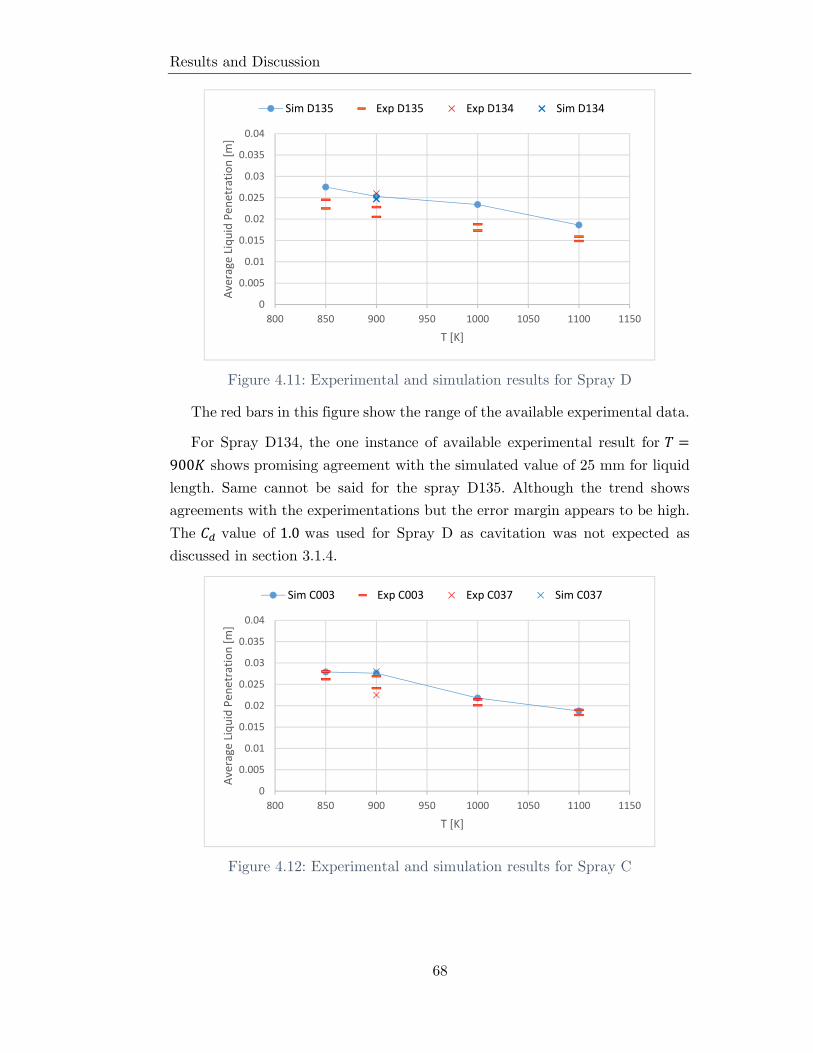
Results and Discussion
68
Figure 4.11: Experimental and simulation results for Spray D
The red bars in this figure show the range of the available experimental data.
For Spray D134, the one instance of available experimental result for 900 shows promising agreement with the simulated value of 25 mm for liquid length. Same cannot be said for the spray D135. Although the trend shows agreements with the experimentations but the error margin appears to be high. The value of 1.0 was used for Spray D as cavitation was not expected as discussed in section 3.1.4.
Figure 4.12: Experimental and simulation results for Spray C
800 850 900 950 1000 1050 1100 1150
0
0.005
0.01
0.015
0.02
0.025
0.03
0.035
0.04
T [K]
Average Liquid Pen
etration [m]
Sim D135 Exp D135 Exp D134 Sim D134
800 850 900 950 1000 1050 1100 1150
0
0.005
0.01
0.015
0.02
0.025
0.03
0.035
0.04
T [K]
Average Liquid Pen
etration [m]
Sim C003 Exp C003 Exp C037 Sim C037

Results and Discussion
69
For Spray C, according to a previous ECN4 study, a value of 0.81 was used and this proved to be in good agreement with the experimental results for C003 but the same cannot be said for C037.
Nonetheless, the study of spray C and D is a good indication of the fidelity of the simulation and applicability of its results in various conditions.
4.4. ECN5 Submissions
Various participating organizations and groups presented their data in the fifth ECN workshop and the general setup for each one is briefly summarized below:
Table 4.5: Summary of ECN5 participants
Institution/ Group CFD code
Turbulence model Spray Modeling Thermodynamics
Aachen-RWTH
CIAO (in-house)
LES Dynamic Smagorinsky
Lagrangian DDM: Initial angle and drop size from DNS primary atomization with no BU model
Ideal fluid EoS and drop evaporation
CMT-UniOvi OpenFOAMRANS standard k-e C1=1.6
Eulerian single fluid Σ-Y: Homogeneous mixture
Ideal fluid EoS and VLE
Politecnico di Milano
OpenFOAMRANS standard k-e C1=1.55
Lagrangian DDM: Blob / KH+RT
Ideal fluid EoS and drop evaporation
TUM/TU Delft
INCA (in-house)
LES ALDM implicit filter
Eulerian single-fluid: Homogeneous mixture
Real fluid cubic EoS and VLE
Comparison of these contributions to the workshop shows some interesting agreements between different approaches to spray simulation as well as some stark areas of disagreement. Politecnico di Milano and CMT results utilized a RANS simulation. Aachen-RWTH used a DNS simulation for the region near the nozzle and switch to LES simulation for the far field. The other LES simulation was performed by TUM which used a real fuel model as opposed to the ideal model used in other simulations.

Results and Discussion
70
The results for liquid penetration, spray mixing line, mixture fraction as a function of axial distance and velocity values from the injector of Spray A from different submissions are presented and discussed in this section. These comparisons could show the benefits or shortcomings of certain simulation methods over others and expose some ideas for further improvements.
Figure 4.13: Liquid penetration results of ECN5 topic 3
Focusing on the macroscopic features of the spray, the figure above shows the simulation results for the average liquid length at various ambient temperatures. The liquid penetration results shows that various spray simulations struggle most at the lower temperature levels and mostly under predict it.
There is a significant uncertainty also present in the experimental results for liquid length measurements. This value is strongly dependent on factors such as the age and status of the internal surface of the nozzle. The case tuning for 900K was done on a difference set of experimental results than the experimental results presented in the figure.
The challenging condition of lower temperature for different approaches to spray simulation also for previous ECN workshops is a good indicator that it might be beneficial to focus on lower temperature ranges and identify a working setup for those conditions. The higher temperature ranges appears to resolve the issue and the prediction from various models fall within closer prediction values of each other.

Results and Discussion
71
Figure 4.14: Mixing Line results of ECN5 topic 3
Comparing the mixing line between the various submissions reveals some interesting characteristics. The 1D adiabatic mixing model results are shown in the form of a dashed line as reference. The scatter plot for various submissions is also presented. An interesting phenomena is the so called “knee” in the mixing line where the data seems to shift backwards. Politecnico and TUM results exhibited this trait at slightly richer mixtures as opposed to CMT results. The Temperature at which the “knee” is observed is rather significant as the temperatures above that threshold (close to 570K) are associated with only the gas phase while below that level both liquid and gas phase are present in the corresponding cell.
One motivation in the reason behind different simulation result for this temperature level could be non-identical fuel properties as well as various methods used to calculate the temperature. Nonetheless, this effect could be the focus of future work.

Results and Discussion
72
Figure 4.15: Mixture fraction as function of axial distance. ECN5
Mixture fraction at various axial locations is another interesting comparison in the data as it exposed another measurement where many simulations seemingly were in agreement except for one (RWTH). This difference is also observed one the mixture fraction is plotted at a fixed axial position as presented in the following figure.
Figure 4.16: Mixture fraction at axial position of 30 mm
RWTH simulation involves a DNS simulation close to nozzle and LES model for further downstream. Their model seems to be under predicting the mixture fraction compared to other data but it should be noted that it captures the regions with lower mixture fraction with better agreement to experimental data.
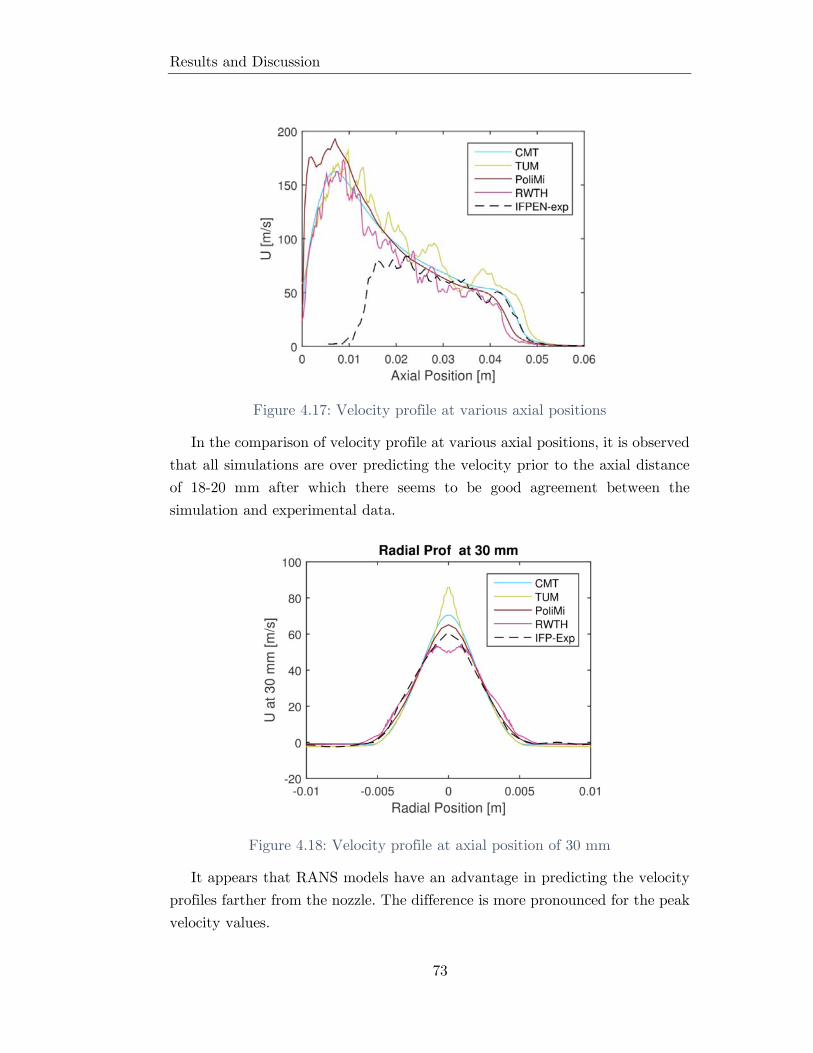
Results and Discussion
73
Figure 4.17: Velocity profile at various axial positions
In the comparison of velocity profile at various axial positions, it is observed that all simulations are over predicting the velocity prior to the axial distance of 18-20 mm after which there seems to be good agreement between the simulation and experimental data.
Figure 4.18: Velocity profile at axial position of 30 mm
It appears that RANS models have an advantage in predicting the velocity profiles farther from the nozzle. The difference is more pronounced for the peak velocity values.

Conclusions
74
Conclusions
Conclusions
A direct injection diesel spray was simulated using a RANS model by means of a Lagrangian-Eulerian approach.
Steady state liquid penetration and vapor phase penetration were selected as the main injector simulation indexes as well as the spray shape visualization using the Lagrangian field and a definition of the spray mixing line was introduced. Parameters of standard - turbulence model, turbulent Schmidt number and the computational grid were studied for their impact on simulation results and modified to better capture the spray phenomena and mixing. Additionally, the blob injection model and a KH/RT breakup model was adopted and the parameters were tuned to match the experimental results of SNL available at Spray A standard conditions.
The same simulation was applied to different injection conditions at various temperatures keeping the same ambient density to observe the effect of ambient temperature on the results. It was observed that the steady state liquid penetration is reduced for higher ambient temperatures where spray evaporation is facilitated. The correlation between mixing line dispersion and validity of simulation results was demonstrated. The simulation results appear to be in good agreement with the experimental data above ambient temperatures of 900K below which the model over predicts the steady state liquid length and exhibits an observable dispersion in the mixing line.
Furthermore, same Spray A simulation parameters were used to simulate Spray C and D conditions with higher nominal nozzle diameter than Spray A and different nozzle shape more prone to flow cavitation inside the nozzle hole. Simulation results show considerable variation form the experimental results and the liquid length was not reliably captured for spray C.
The results were presented as contribution to the fifth ECN workshop along with contribution of other institutions and groups for the third topic of the
Conclusions
75
workshop regarding non-reactive diesel spray mixing and evaporation. The discrepancies in the simulation results shows the sensitivity of such simulations to the models embedded and the simulation parameters.
Most simulations predict the liquid length of the Spray A with good accuracy but the uncertainty in the experimental data makes this comparison more difficult. The liquid length seems to be under predicted at lower temperature levels for most simulation results but at higher temperature levels the results are in better agreement with experimentations. As for the vapor phase penetration, the simulation results show better consistency regardless of the model used and better results are obtained also for lower temperature values. With respect to other measurements such as mixture fraction or velocity field at various axial distances from the nozzle, there appears to be variability between the predictions of different models. This discrepancy is more pronounced if we focus our attention to the jet front as opposed to the entire spray global features and it appears that the averaging schemes of RANS and LES provide different predictions with respect to variables such as the mixture fraction. Simulations of Spray C and D were able to predict the difference in penetration values and distinguish between the two sprays but they showed considerable margins of error with respect to experimental data.
Considering the future work on this topic, it appears that focusing on macroscopic features of the spray such as liquid length and vapor phase penetration does not provide a good picture of the simulation accuracies. Despite the attention to spray mixing line, other indexes could be interesting in model tuning. Some motivations based on simulation results of this work as well as previous ECN workshops include examining the SMD values at certain axial distances and a focus on model tuning for lower temperatures. As for Spray C and D, the involved cavitation could call for a modified atomization approach and further study of those specific sprays and performing case tuning could prove beneficial.

76
Bibliography
Bibliography
[1] G. Ferrari, Motori a combustione interna. Società Editrice Esculapio, 2016.
[2] A. H. Lefebvre and V. G. McDonell, Atomization and sprays. CRC press, 2017.
[3] S. K. Mahapatra and K. C. Ratha, "Paris Climate Accord: Miles to Go," Journal of International Development, vol. 29, no. 1, pp. 147-154, 2017.
[4] K. Burton, J. L. Whitelaw, A. L. Jones, and B. Davies, "Are respiratory protection standards protecting worker health against ultrafine diesel particulate matter emissions? An Australian perspective," 2016.
[5] J. B. Brower, M. Doyle-Eisele, B. Moeller, S. Stirdivant, J. D. McDonald, and M. J. Campen, "Metabolomic changes in murine serum following inhalation exposure to gasoline and diesel engine emissions," Inhalation Toxicology, vol. 28, no. 5, pp. 241-250, 2016/04/15 2016.
[6] N. Kumar, S. L. Soni, D. Sharma, and A. K. Srivastava, "Performance evaluation and emission analysis of variable compression ratio direct injection diesel engine," MATTER: International Journal of Science and Technology, vol. 2, no. 2, 2016.
[7] S. Hoseini, G. Najafi, B. Ghobadian, R. Mamat, N. A. C. Sidik, and W. Azmi, "The effect of combustion management on diesel engine emissions fueled with biodiesel-diesel blends," Renewable and Sustainable Energy Reviews, vol. 73, pp. 307-331, 2017.
[8] F. Payri, J. V. Pastor, R. Payri, and J. Manin, "Determination of the optical depth of a DI diesel spray," Journal of Mechanical Science and Technology, vol. 25, no. 1, pp. 209-219, 2011.
[9] C. Baumgarten, Mixture formation in internal combustion engines. Springer Science & Business Media, 2006.

Bibliography
77
[10] A. Hamzah, F. Poursadegh, J. Lacey, P. Petersen, M. Brear, and R. Gordon, "A comparison of diffuse back-illumination (DBI) and Mie-scattering technique for measuring the liquid length of severely flashing spray," 2016.
[11] P. Nordin, Complex chemistry modeling of diesel spray combustion. Chalmers University of Technology, 2001.
[12] Engine Combustion Network [Website]. Available: https://ecn.sandia.gov/
[13] W. Chiu, S. Shahed, and W. Lyn, "A transient spray mixing model for diesel combustion," SAE Technical Paper0148-7191, 1976.
[14] H. Hiroyasu and T. Kadota, "Models for combustion and formation of nitric oxide and soot in direct injection diesel engines," SAE Technical Paper0148-7191, 1976.
[15] D. Adler and W. Lyn, "The evaporation and mixing of a liquid fuel spray in a diesel air swirl," in Proceedings of the Institution of Mechanical Engineers, Conference Proceedings, 1969, vol. 184, no. 10, pp. 171-180: SAGE Publications.
[16] R. B. Melton, "Diesel fuel injection viewed as a jet phenomenon," SAE Technical Paper0148-7191, 1971.
[17] R. Reitz and C. Rutland, "Development and testing of diesel engine CFD models," Progress in Energy and Combustion Science, vol. 21, no. 2, pp. 173-196, 1995.
[18] G. Stiesch, Modeling engine spray and combustion processes. Springer Science & Business Media, 2013.
[19] M. W. Chase, "JANAF thermochemical tables," JANAF thermochemical tables, by Chase, MW Washington, DC: American Chemical Society; New York: American Institute of Physics for the National Bureau of Standards, c1986.. United States. National Bureau of Standards., 1986.
[20] A. Gosman and D. Clerides, "Diesel spray modelling: a review," Proceedings of ILASS-Europe, Florence, Italy, 1997.
[21] G. M. Magnotti and C. L. Genzale, "A Novel Approach to Assess Diesel Spray Models using Joint Visible and X-Ray Liquid Extinction Measurements," SAE International Journal of Fuels and Lubricants, vol. 8, no. 2015-01-0941, pp. 167-178, 2015.
[22] R. D. Reitz and R. Diwakar, "Structure of high-pressure fuel sprays," SAE Technical Paper0148-7191, 1987.
[23] G. Taylor, "The instability of liquid surfaces when accelerated in a direction perpendicular to their planes. I," in Proceedings of the Royal

Bibliography
78
Society of London A: Mathematical, Physical and Engineering Sciences, 1950, vol. 201, no. 1065, pp. 192-196: The Royal Society.
[24] L. M. Pickett, J. Manin, A. Kastengren, and C. Powell, "Comparison of near-field structure and growth of a diesel spray using light-based optical microscopy and x-ray radiography," SAE International Journal of Engines, vol. 7, no. 2014-01-1412, pp. 1044-1053, 2014.
[25] Y. Pei, M. J. Davis, L. M. Pickett, and S. Som, "Engine Combustion Network (ECN): Global sensitivity analysis of Spray A for different combustion vessels," Combustion and Flame, vol. 162, no. 6, pp. 2337-2347, 2015/06/01/ 2015.
[26] J. Gimeno, G. Bracho, P. Martí-Aldaraví, and J. E. Peraza, "Experimental study of the injection conditions influence over n-dodecane and diesel sprays with two ECN single-hole nozzles. Part I: Inert atmosphere," Energy Conversion and Management, vol. 126, pp. 1146-1156, 2016.
[27] C. J. Greenshields, "Openfoam user guide," OpenFOAM Foundation Ltd, version, vol. 3, no. 1, 2015.
[28] T. Lucchini and G. D’Errico, "Diesel spray simulations using OpenFOAM and Lib-ICE," in "OpenFOAM Foundation Ltd, version," Politecnico di Milano, Internal Combustion Engine Group2013, vol. 3.
[29] A. Andriotis, M. Gavaises, and C. Arcoumanis, "Vortex flow and cavitation in diesel injector nozzles," Journal of Fluid Mechanics, vol. 610, pp. 195-215, 2008.
[30] H. G. Weller, G. Tabor, H. Jasak, and C. Fureby, "A tensorial approach to computational continuum mechanics using object-oriented techniques," Computers in physics, vol. 12, no. 6, pp. 620-631, 1998.
[31] The OpenFOAM Foundation [Website]. Available: https://openfoam.org/
[32] T. Lucchini, G. D’Errico, and D. Ettorre, "Numerical investigation of the spray–mesh–turbulence interactions for high-pressure, evaporating sprays at engine conditions," International Journal of Heat and Fluid Flow, vol. 32, no. 1, pp. 285-297, 2011.
[33] F. P. Joshua Lacey, Michael Brear, Robert Gordon, "Characterising the Liquid Length of Multi-hole GDI Sprays Using Diffuse Back-Illumination," Asia Pacific Automotive Engineering Conference APAC, 2015.
[34] J. D. Naber and D. L. Siebers, "Effects of gas density and vaporization on penetration and dispersion of diesel sprays," SAE technical paper0148-7191, 1996.

Bibliography
79
[35] C. Kurvers and C. Luijten, "Real Gas Effects in Siebers' Mixing-Limited Spray Vaporization Model," SAE Technical Paper0148-7191, 2010.
[36] J. Gacia-Oliver, J. Pastor, A. Pandal, N. Trask, E. Baldwin, and D. Schmidt, "Diesel Spray CFD Simulations Based on the Sigma-Y Eulerian Atomizaton Model," Atomization and Sprays, vol. 23, pp. 71-95, 2013.
[37] A. Wierzba, "Deformation and breakup of liquid drops in a gas stream at nearly critical Weber numbers," Experiments in Fluids, vol. 9, no. 1, pp. 59-64, 1990.
[38] U. Ayachit, "The Paraview Guide," Kitware Inc, 2015.
[39] K. Moreland, "The paraview tutorial," Sandia National Laboratories, Tech. Rep. SAND, 2013.
[40] L. M. Pickett et al., "Comparison of Diesel Spray Combustion in Different High-Temperature, High-Pressure Facilities," SAE Int. J. Engines, vol. 3, no. 2, pp. 156-181, 2010.
[41] D. L. Siebers, "Scaling liquid-phase fuel penetration in diesel sprays based on mixing-limited vaporization," SAE technical paper0148-7191, 1999.
[42] R. Payri, J. Gimeno, J. Cuisano, and J. Arco, "Hydraulic characterization of diesel engine single-hole injectors," Fuel, vol. 180, pp. 357-366, 9/15/ 2016.
[43] A. L. Kastengren et al., "Engine combustion network (ECN): measurements of nozzle geometry and hydraulic behavior," Atom. Sprays, vol. 22, no. 12, pp. 1011-1052, 2012.
[44] Q. Xue et al., "Eulerian CFD modeling of coupled nozzle flow and spray with validation against X-ray radiography data," SAE International Journal of Engines, vol. 7, no. 2014-01-1425, pp. 1061-1072, 2014.
[45] Y. Tominaga and T. Stathopoulos, "Turbulent Schmidt numbers for CFD analysis with various types of flowfield," Atmospheric Environment, vol. 41, no. 37, pp. 8091-8099, 2007.
[46] D. Valero and D. B. Bung, "Sensitivity of turbulent Schmidt number and turbulence model to simulations of jets in crossflow," Environmental Modelling & Software, vol. 82, pp. 218-228, 2016.
[47] "ECN Workshop Proceedings," 2014-2015: Engine Combustion Network.