Embed Size (px)
Citation preview
J. Non-Newtonian Fluid Mech., 74 (1998) 47–88
Numerical simulation of extensional deformations of viscoelasticliquid bridges in filament stretching devices
Minwu Yao a,*, Gareth H. McKinley b
a Ohio Aerospace Institute, 22800 Cedar Point Road, Brook Park, OH 44142, USAb Di6ision of Applied Sciences, Har6ard Uni6ersity, Cambridge, MA 02138, USA
Received 5 December 1996
Abstract
Large extensional deformations of viscoelastic fluid columns in filament stretching rheometers are studied throughnumerical simulations up to Hencky strains of greater than o=4. The time-dependent axisymmetric calculationsincorporate the effects of viscoelasticity, surface tension, fluid inertia, plus a deformable free surface and providequantitative descriptions of the evolution in the filament profile, the kinematics in the liquid column and the resultingdynamic evolution in the viscous and elastic contributions to the total stress. In addition to investigating the variationin the apparent Trouton ratio expected in experimental measurements using this new type of extensional rheometer,we also investigate the generic differences between the response of Newtonian and viscoelastic fluid filamentsdescribed by the Oldroyd-B model. For small strains, the fluid deformation is governed by the Newtonian solventcontribution to the stress and the filament evolution is very similar in both the Newtonian and viscoelastic cases.However, in the latter case at large strains and moderate Deborah numbers, elastic stresses dominate leading tostrain-hardening in the axial mid-regions of the column and subsequent drainage of the quasi-static liquid reservoirthat forms near both end-plates. These observations are in good qualitative agreement with experimental observa-tions. For small initial aspect ratios and low strains, the non-homogeneous deformation predicted by numericalsimulations is well described by a lubrication theory solution. At larger strains, the initial flow non-homogeneity leadsto the growth of viscoelastic stress boundary layers near the free surface which can significantly affect the transientTrouton ratio measured in the device. Exploratory design calculations suggest that mechanical methods for modifyingthe boundary conditions at the rigid end-plates can reduce this non-homogeneity and lead to almost ideal uniaxialelongational flow kinematics. © 1998 Elsevier Science B.V.
Keywords: Extensional flow; Fluid dynamics; Finite element method; Liquid bridge; Filament stretching device;Viscoelasticity; Oldroyd-B fluid; Moving boundary problem
* Corresponding author. Tel.: +1 216 9623094; fax: +1 216 9623120.
0377-0257/98/$19.00 © 1998 Elsevier Science B.V. All rights reserved.PII S0377 -0257 (97 )00052 -9
M. Yao, G.H. McKinley / J. Non-Newtonian Fluid Mech. 74 (1997) 47–8848
1. Introduction
The key to a better understanding of the extensional behavior of polymer liquids in complexflows is the accurate, unambiguous quantitative measurement of extensional rheological materialproperties [1]. Filament stretching devices are one of the most promising techniques that havebeen developed for providing accurate measurements of transient elongational stress growthfunctions for viscous polymer solutions [2]. Such filament stretching devices are currently beingdeveloped by several independent research groups around the world and in the present paper werefer extensively to the work of Sridhar and Tirtaatmadja [3,4], Kroger, Berg et al. [5,6],Solomon and Muller [7], and McKinley and Spiegelberg et al. [8–10]. In the filament stretchingapparatus, a cylindrical liquid column is first generated between two concentric circular platesand then is elongated by pulling one or both of the end-plate fixtures at an exponentiallyincreasing rate. It is hoped that the resulting flow kinematics in the liquid column approximatean ideal uniaxial elongational flow, and the extensional viscosity is determined from the axialforce at the end-plate which is measured as a function of time [11].
The major problems with the conventional filament stretching configuration are: (i) thepresence of a deformable free surface and (ii) the two rigid, non-deforming end-plates. Theformer leads to a significant ‘necking’ in the central region of liquid bridge due to the surfacetension of the fluid and the latter results in an appreciable shear component in the deformationhistory due to the no-slip boundary condition at the rigid end-plates. As a result the elongationis not shear-free, the extension rate is spatially and temporally inhomogeneous and analysis ofthe experimental results does not lead to true extensional material properties, but an ‘apparentextensional viscosity’ [2].
To overcome the experimental difficulties, two approaches that modify the fluid kinematics insuch devices have been proposed in the literature. One is the velocity compensation algorithmwhich was first successfully used by Tirtaatmadja and Sridhar [4] and more recently bySpiegelberg et al. [9]. In this approach the imposed velocity at the moving plate is modified insuch a way that a constant ‘effective’ extension rate, defined on the basis of the measured radiusand velocity at the mid-plane of the filament, can be achieved at the axial mid-section of thefilament. This strategy provides more accurate extensional rheological measurements despite thefact that the extension rate in the liquid column remains spatially inhomogeneous along theaxial direction as we show below in our numerical results. The second approach focuses ongenerating homogeneous uniaxial elongational kinematics by simultaneously elongating thesample axially and reducing the diameter of the end-plate fixtures at an exponential rate. Sincethe imposed axial and radial velocity components at the two end-plates provide the boundaryconditions necessary for homogeneous uniaxial elongational flow, this approach in theory leadsto a perfect cylindrical fluid column and a constant extensional strain rate both in space andthroughout the duration of the test. At large strains, the cylindrical fluid column rapidly exceedsthe static stability criterion of Rayleigh L]2pR [8]; however, as we show below, capillarybreak-up is greatly retarded as a result of the high viscosity of the fluid column. This latterapproach will be referred to as a reducing diameter device (RDD) herewith. Experiments witha RDD were first carried out by Berg et al. [6] under microgravity conditions. One inherent limitwith such a RDD is that the radial engineering strain (defined by the ratio of ultimate diameterover the initial diameter) that can be achieved is usually restricted by the mechanical design of
M. Yao, G.H. McKinley / J. Non-Newtonian Fluid Mech. 74 (1998) 47–88 49
the instrument to be much lower than the total axial strain of the experiment. In the experimentsof Berg et al., a final reduction ratio of two was achieved (namely the end-plate diameter wasreduced by half at the end of experiments). In the present work, we investigate the consequencesof such limitations and explore possible enhancement in the accuracy of the measured materialproperties that may be achieved by increasing the final reduction ratio of a mechanical RDD.
Despite the rapid proliferation of filament stretching rheometers, there are few theoreticalstudies of these devices. Broad qualitative agreement between experimental measurements of asingle fluid in different laboratories has been demonstrated [4,9], and the measurements havebeen fitted with single and multi-mode formulations of viscoelastic constitutive models [12].However, observations have shown that the geometric configuration of the device can affect thefluid kinematics and the dynamical evolution in the tensile force [9] and also lead to the onsetof elastic flow instabilities [10]. Large discrepancies between the measured material functions atlarge strains and the asymptotic steady state value estimated from molecular considerations havealso been noted [13]. Before new constitutive models are sought, however, it is necessary toverify through numerical calculation that the device is behaving as expected. Similar calculationsfor other extensional flow devices, such as opposed jet rheometers have revealed that largedeviations from the expected kinematics can exist even for Newtonian fluids [14,15]. Suchsimulations can also be used to guide the design of future versions of the device.
In this work, we study the dynamic response of axisymmetric viscoelastic liquid bridges in afilament stretching device. As a moving boundary problem, the analysis of the liquid bridgerequires three key elements: deformable free surface capabilities, a robust transient algorithmand appropriate constitutive models. Dynamic analysis of the transient free-boundary motion ofa non-Newtonian material is computationally challenging. In the literature, relatively little work,either theoretical or numerical, has been reported so far even for the case of Newtonian fluids.Analytical solutions are available only under certain restrictive presumptions, and numericalsolutions have been limited to small total deformations. In an early numerical study [16],Shipman et al. simulated one of the low-rate falling-plate extensional rheometer experimentsconducted by Sridhar and co-workers using a free-surface finite element method and theOldroyd-B constitutive model. A reasonable agreement in free surface shapes with the experi-ment was obtained. However, computational restrictions introduced several ambiguities in theirmodel. First, the finite element mesh was constrained to a fixed axial length and consequentlyonly a part of the deforming domain was modeled. Second, at the truncated boundary, thetheoretical steady-state extensional stress was used to approximate the unknown stress boundarycondition. The third ambiguity was introduced by neglecting the effects of fluid outside the fixedcontrol volume. Finally, the simulation was not started at t=0, but at t=2.42 s, whileequilibrium initial conditions for the polymeric stress were used and hence any effects of theinitial configuration of the device were not captured. In another numerical investigation [8],Gaudet et al. used the boundary element method to perform a dynamic analysis of Newtonianliquid bridges for a wide range of aspect ratios and capillary numbers. In their work, the fluidmotion was assumed to be quasi-steady by neglecting the inertia terms in the momentumequation and the fluid motion was governed by the linear Stokes equations. The viscous forceexerted by the fluid on the stationary end-plate was computed as a function of strain; however,in this study the end-plates were separated linearly in time rather than in the exponential manneremployed in filament stretching rheometers. In a more recent work [29], Sizaire and Legat
M. Yao, G.H. McKinley / J. Non-Newtonian Fluid Mech. 74 (1997) 47–8850
studied the extensional response of the Boger fluid in the filament stretching devices using anapproximate version of the finitely extensible non-linear elastic dumbbell model modified byChilcott and Rallison (FENE-CR). The inertia and gravity effects were neglected in theirfree-surface finite element solutions for the viscoelastic moving boundary problem and theresults were compared with the experimental measurements by Spiegelberg and McKinley. Goodqualitative agreement with the experiments was found, however, the spatial and temporalinhomogeneity of the kinematics generated by the device were not investigated in detail.
The present study is based on an axi-symmetric model of the liquid bridge which incorporatesthe viscoelastic behavior of the liquid, surface tension, fluid inertia, a deformable free surfaceand imposed extensional deformations. The primary goals of the present work are: to study thecomplex time-dependent extensional deformations in filament stretching devices, to compare andcontrast differing fluid response for viscoelastic and Newtonian liquid samples, to investigate theeffects of initial geometric configuration of the filament, to examine the benefits of adaptivediameter end-plates in minimizing non-homogeneous kinematics within fluid column, and toprovide a numerical tool to aid in optimization of experimental designs.
2. Mathematical model
2.1. Description of the problem
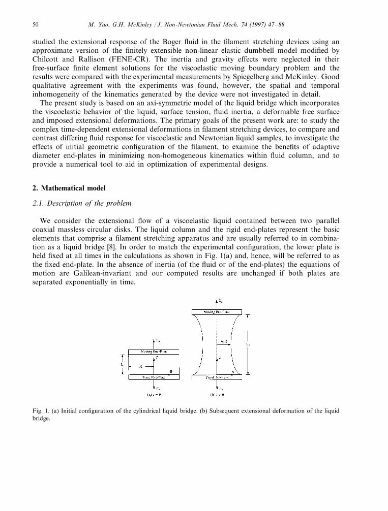
We consider the extensional flow of a viscoelastic liquid contained between two parallelcoaxial massless circular disks. The liquid column and the rigid end-plates represent the basicelements that comprise a filament stretching apparatus and are usually referred to in combina-tion as a liquid bridge [8]. In order to match the experimental configuration, the lower plate isheld fixed at all times in the calculations as shown in Fig. 1(a) and, hence, will be referred to asthe fixed end-plate. In the absence of inertia (of the fluid or of the end-plates) the equations ofmotion are Galilean-invariant and our computed results are unchanged if both plates areseparated exponentially in time.
Fig. 1. (a) Initial configuration of the cylindrical liquid bridge. (b) Subsequent extensional deformation of the liquidbridge.
M. Yao, G.H. McKinley / J. Non-Newtonian Fluid Mech. 74 (1998) 47–88 51
The initial configuration of the liquid bridge is a cylinder when t50−. Let R0 denote theradius of the two equal end-plates and L0 the initial separation between the two end-plates. Theinitial aspect ratio of the liquid bridge is then defined as
L0 L0/R0. (1)
At the instant t=0+, the top plate is set into motion which results in a transient extensionaldeformation of the liquid column as depicted schematically in Fig. 1(b). The fluid column isassumed to remain axisymmetric and to wet the end-plate at all times. The contact line is thuspinned to the radial edges of the disks. This agrees with experimental observations of the fluidconfiguration near the end-plates, except at very high tensile stresses and large strains [10].During the deformation, the dynamic length of the liquid bridge is denoted by Lp(t) and thetransient aspect ratio
Lt Lp(t)/R0 (2)
increases with time while the volume of the liquid bridge remains constant. The top plate willbe referred to as the moving end-plate and its axial velocity is L: p=dLp/dt. In this study, we areparticularly interested in the exponential separation between the two end-plates which isprescribed by
Lp(t)=L0eo; 0t and L: p(t)=L0o; 0e o; 0t, (3)
where o; 0 is the imposed constant extension rate, and (L0o; 0) V0 is the initial velocity of themoving end-plate.
2.2. Go6erning equations
The fluid flow within the liquid bridge is assumed to be isothermal, incompressible andaxi-symmetric and is governed by the incompressibility condition and the equations of motion:
9 ·u=0, (4)
r�(u(t
+u ·9u�
=9 ·T+F. (5)
Here r is the density, u is the velocity vector, F is the body force and T is the Cauchy stresstensor
T −pI+t, (6)
where p is an isotropic pressure, I is the unit tensor and t is the extra stress tensor. In this work,we consider the simplest generally admissible differential constitutive model for polymersolutions, the convected Jeffreys model [11] or Oldroyd-B model [17]. In this model, the solventcontribution ts and the polymeric contribution tp to the extra stress are defined as
t=ts+tp, (7)
ts=2hsD, (8)
M. Yao, G.H. McKinley / J. Non-Newtonian Fluid Mech. 74 (1997) 47–8852
tp+l1�(tp
(t+u ·9tp− (9u)T ·tp−tp · (9u)
n=2hpD, (9)
where the rate-of-strain tensor is defined as
D 12[9u+ (9u)T], (10)
and the three physical parameters involved in this model are the solvent viscosity hs, the polymercontribution to the viscosity hp and the fluid relaxation time l1.
At large strains, experiments [4,9] suggest that finite extensibility of the macromolecules maylead to an asymptotic or steady state value in the extensional stresses. Such effects can becaptured numerically by incorporating a finitely extensible nonlinear elastic (FENE) spring intothe kinetic theory leading to Eqs. (7)–(9). However for realistic values of L�50 (L representsthe ratio of the length of a fully extended dumbbell to its equilibrium length), the FENEnonlinearity does not affect the evolution of the filament until large strains o\4 [9]. Since weare primarily interested in a general understanding the basic differences between Newtonian andviscoelastic fluid samples, we therefore do not consider finite extensibility in the present work.
The complete boundary conditions for this problem include: the no-slip condition along theinterface between the liquid and the end-plates, axi-symmetric along the z-axis, the prescribedmotion given by Eq. (3) at the moving end-plate, and the following kinematic and dynamicconditions
(S(t
+u ·9S=0, (11)
T ·n= (2sH−pa)n, (12)
on the deformable free surface boundary. Here S(r, z, t) [R(z, t)−r ]=0 is a function thatdefines the spatial position of the free surface R(z, t), n is the unit norm of the surface, pa is theambient pressure, H is the mean Gaussian curvature of the free surface and s is the surfacetension coefficient. In addition, the following initial conditions for the velocity, pressure andextra stress fields:
u(r, z)=0, p(r, z)−pa=0 and t(r, z)=0 at t50−, (13)
also need to be imposed. Eqs. (4)–(13) plus the boundary conditions form a well-posed set ofgoverning equations for the moving boundary problem of viscoelastic liquid bridges.
2.3. Dimensionless scaling
We choose to scale lengths and time with the initial radius R0 and the imposed stretch rate1/o; 0, respectively. Stresses and pressures are scaled with h0o; 0 where h0=hs+hp is the totalviscosity of the fluid and velocities are nondimensionalized with the product o; 0R0. In addition tothe geometric aspect ratio L0 defined in Eq. (1) and the Hencky strain o=o; 0t imposed on thefilament, the following dimensionless groups are also important in governing the relativemagnitude of each force affecting the evolution of the liquid bridge:
The Deborah number
De l1o; 0, (14)
M. Yao, G.H. McKinley / J. Non-Newtonian Fluid Mech. 74 (1998) 47–88 53
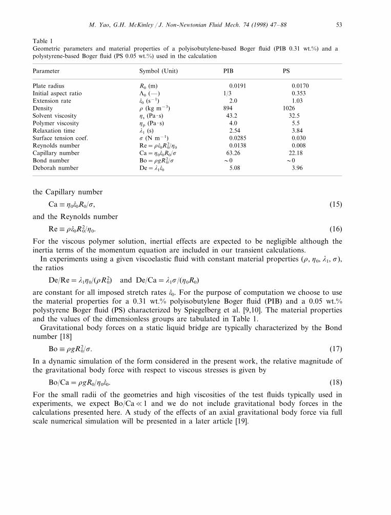
Table 1Geometric parameters and material properties of a polyisobutylene-based Boger fluid (PIB 0.31 wt.%) and apolystyrene-based Boger fluid (PS 0.05 wt.%) used in the calculation
PIBParameter Symbol (Unit) PS
0.0191 0.0170R0 (m)Plate radius1/3Initial aspect ratio L0 (—) 0.353
1.032.0o; 0 (s−1)Extension rate1026Density r (kg m−3) 894
32.5Solvent viscosity hs (Pa · s) 43.24.0Polymer viscosity hp (Pa · s) 5.52.54 3.84l1 (s)Relaxation time0.0285Surface tension coef. 0.030s (N m−1)
0.0080.0138Re=ro; 0R20/h0Reynolds number
22.18Capillary number Ca=h0o; 0R0/s 63.26�0Bond number Bo=rgR0
2/s �05.08Deborah number 3.96De=l1o; 0
the Capillary number
Ca h0o; 0R0/s, (15)
and the Reynolds number
Re ro; 0R20/h0. (16)
For the viscous polymer solution, inertial effects are expected to be negligible although theinertia terms of the momentum equation are included in our transient calculations.
In experiments using a given viscoelastic fluid with constant material properties (r, h0, l1, s),the ratios
De/Re=l1h0/(rR20) and De/Ca=l1s/(h0R0)
are constant for all imposed stretch rates o; 0. For the purpose of computation we choose to usethe material properties for a 0.31 wt.% polyisobutylene Boger fluid (PIB) and a 0.05 wt.%polystyrene Boger fluid (PS) characterized by Spiegelberg et al. [9,10]. The material propertiesand the values of the dimensionless groups are tabulated in Table 1.
Gravitational body forces on a static liquid bridge are typically characterized by the Bondnumber [18]
Bo rgR20/s. (17)
In a dynamic simulation of the form considered in the present work, the relative magnitude ofthe gravitational body force with respect to viscous stresses is given by
Bo/Ca=rgR0/h0o; 0. (18)
For the small radii of the geometries and high viscosities of the test fluids typically used inexperiments, we expect Bo/Ca�1 and we do not include gravitational body forces in thecalculations presented here. A study of the effects of an axial gravitational body force via fullscale numerical simulation will be presented in a later article [19].
M. Yao, G.H. McKinley / J. Non-Newtonian Fluid Mech. 74 (1997) 47–8854
2.4. Calculation of Trouton ratio
One of the primary goals of the filament stretching experiment is to measure the extensionalviscosity as a function of Hencky stain. For the ideal uniaxial elongational flow, the extensionalviscosity is defined as
hE(o; 0, t) (tzz−trr)/o; 0, (19)
where tzz, trr are the normal components of the extra stress defined in Eq. (7). The Hencky straino used in this paper is determined from the displacement of the moving end-plate. For theexponential separation rate, we have
o o; 0t= ln(Lp/L0). (20)
Calculations of the extensional viscosity, or equivalently the transient Trouton ratio, are usuallybased on the measured axial force at the end-plate, Fz. The fundamental theoretical results basedon the homogeneous stresses in the uniaxial elongational flow are given by
Tzz+p0=tzz−trr=hEo; 0, (21)
where p0 is the ambient pressure. For a cylindrical fluid filament with a uniform radius R, thefollowing relationship can be obtained by integrating Eq. (21) over the circular area of the endsurface of the liquid column
hE=Fz
pR2o; 0, (22)
which relates hE directly to Fz. In our calculations, the normal force is obtained by the followingintegral
Fz(t)=&
A
[Tzz(r, z=0, t)+p0] dA=Fp+Fv+Fe, (23)
where A is the circular domain of the end-plate; Fp, Fv and Fe are pressure, viscous and polymer(elastic) contributions to the normal force, respectively.
The original derivation of Eq. (21) involves the following assumptions [11]: (1) incompressibleNewtonian fluid; (2) ideal uniaxial elongational flow with homogeneous extension rate and extrastress; (3) steady state with negligible inertia efffects, i.e. (u/(t=0 and u ·9u=0; (4) no externalforces. In practice, the basic relationship Eq. (22) has been generalized to the following form[4,8,9]
Tr hE
h0=
Fz
h0o; 0pR2mid
−s
h0o; 0Rmid+O(Fi, Fg), (24)
where Rmid denotes the radius of the fluid filament at the axial mid-plane z=Lp(t)/2 and thesecond term in the right hand side is the surface tension correction term. The final term O(Fi, Fg)accounts for the corrections due to the inertia force Fi and gravitational force Fg, respectively.In the results presented in this paper, this last term is assumed to be negligibly small. Detailedstudies of the inertia and gravity corrections will be pursued in later publications. Note that theuse of Rmid in Eq. (24) implies that the calculated Tr pertains specially to the mid-plane for
M. Yao, G.H. McKinley / J. Non-Newtonian Fluid Mech. 74 (1998) 47–88 55
non-homogeneous flow situations. In the ideal uniaxial elongational flow of a Newtonian fluid,the Trouton ratio is known to be simply a constant of Tr=3.
3. Numerical simulation
3.1. Finite element method
Two finite element domains are considered in this study. The first model uses a computationaldomain bounded by 05r5R(z, t) and 05z5Lp(t). Since this model considers the wholelength of the liquid bridge, it will be referred to as the whole-length model. The second modelfurther assumes symmetry with respect to the mid-plane between the two end-plates. Conse-quently, the computational domain is defined by 05r5R(z, t) and 05z5Lp(t)/2 and we referto this configuration as the half-length model. Since the convective inertia forces arising from theu ·9u term are, in general, not symmetric, the half-length model is only valid for small Reynoldsnumbers and small strains.
3.2. Numerical solution
The governing equations are solved using the code POLYFLOW, a commercial finite elementmethod (FEM) program primarily designed for the analysis of flow problems dominated bynon-linear viscous phenomena and viscoelastic effects. The details of the FEM formulation andnumerical techniques used in POLYFLOW are documented in [20]. Galerkin’s method isadopted in the FEM discretization for the momentum equations, and the axi-symmetric FEMmesh is built with the 9-node quadratic quadrilateral element, in which velocity and extra stressare approximated by quadratic shape functions. The pressure is approximated as piecewiselinear (i.e. discontinuous on inter-element boundaries). The coordinates of the free surfaceboundary are interpolated by piecewise linear functions. The transient problem is solved by apredictor–corrector time integration scheme in which the backward Euler method is selected forthe corrector. At each time step, the non-linear algebraic system resulting from the FEMdiscretization is solved by the Newton–Raphson iteration scheme. The non-linear iterationtermination is controlled by a specified iteration convergence tolerance of 10−5 for the relativeerror norms of residuals of the governing equations and free surface update.
Another important aspect for moving boundary problems is the remeshing technique whichcontrols mesh deformation by relocating internal nodes according to the displacement ofboundary nodes in order to avoid unacceptable element distortions. The Thompson transforma-tion remeshing rule [21] is used in this work. Based on the resolution of a partial differentialequation of the elliptic type, the Thompson remeshing technique remains robust even for verylarge mesh deformations.
3.3. Benchmark test
As a moving boundary problem, the dynamic analysis of liquid bridges is difficult, because thespatial position of the free surface, on which the kinematic and dynamic boundary conditions
M. Yao, G.H. McKinley / J. Non-Newtonian Fluid Mech. 74 (1997) 47–8856
are to be applied, is usually unknown a priori and must be solved for as a part of the solution.Consequently, there is, in general, no closed-form (analytical) solution available. Due to the lackof available numerical results to compare our simulations with, it is necessary to conductbenchmark tests in order to check the accuracy of the numerical solutions.
One of the tests considered in this work is the dynamic elongation of a filament with reducingdiameter devices (RDD) at both end-plates. In this test, we consider a liquid bridge of a PIBBoger fluid with an initial cylindrical configuration schematically shown in Fig. 1(a). The initialvalues of velocity, pressure and extra stress are assumed to be zero. The geometry and thematerial parameters of the PIB Boger fluid are tabulated in Table 1. At t=0+, the liquid bridgeis elongated from the moving end-plate by imposing the exponential velocity profile given in Eq.(3) while the other end-plate is held stationary. In addition, the radius of both end-plates isreduced simultaneously by specifying the following radial velocity condition: ur= −0.5o; 0r at thetwo end-plates. The free surface is still treated as a moving boundary and its position in spaceis solved as a direct unknown along with other field variables. Since the imposed axial and radialvelocities at the two end-plates correspond to the boundary conditions of an ideal uniaxialelongational flow, the test results in a perfect cylindrical free surface and homogeneousextensional deformation history throughout the duration of the simulation. This model testproblem is also equivalent to solving the transient start-up of ideal uniaxial elongational flow viaa Lagrangian approach. For the Oldroyd-B fluid, the analytical solution is available [11] andhence can be used for validation purposes.
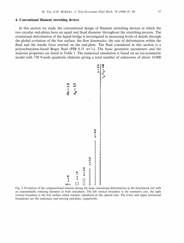
Numerical solutions were obtained using POLYFLOW with 40 quadratic elements. Althoughthe implicit backward time integration scheme was used, a small time-step size corresponding toDo=o; 0 Dt=0.002 was found to be necessary in order to ensure that the relative errors of theaxial deformation of the moving end-plate and radial deformation of the free surface remainedless than 1%. The extensional deformations at several typical strain levels are shown in Fig. 2.The free surface does not deflect in this special case. Nevertheless, due to the exponentiallyincreasing velocity of the upper plate, the liquid bridge experiences large extensional deforma-tion in both axial and radial directions. The axial deformation ratio reaches Lp/L0:148 at astrain level of 5. Since high Hencky strain levels o]5 need to be attained experimentally toinvestigate the extensional rheological behavior of polymer liquids, the results shown in Fig. 2also illustrate one of the great challenges in the liquid bridge modeling, namely the remeshingcapabilities for large extensional deformations. To check how the numerical solution quantita-tively agrees with the available analytical solution, we present comparison plots of the radialdeformation of the free surface versus Hencky strain in Fig. 3(a) and the computed Troutonratio in Fig. 3(b), respectively. As can be seen from Fig. 3, the agreement between theory andthe calculation is excellent and the Trouton ratio is initially Tr(0+)=3hs/h0=2.75 andsubsequently increases exponentially without bound as expected theoretically. The curve denotedby ‘Theory’ in Fig. 3 is based on the following analytical solution [11]:
hE=3hs+2hp
1−2l1o; 0[1−e− (1−2l1o; 0)t/l1]+
hp
1+l1o; 0[1−e− (1+l1o; 0)t/l1], (25)
for the start-up uniaxial elongational flow with an imposed extension rate o; 0.
M. Yao, G.H. McKinley / J. Non-Newtonian Fluid Mech. 74 (1998) 47–88 57
4. Conventional filament stretching devices
In this section we study the conventional design of filament stretching devices in which thetwo circular end-plates have an equal and fixed diameter throughout the stretching process. Theextensional deformation of the liquid bridge is investigated in increasing levels of details throughthe global evolution of the free surface, the flow kinematics, the rate of deformation within thefluid and the tensile force exerted on the end-plate. The fluid considered in this section is apolyisobutylene-based Boger fluid (PIB 0.31 wt.%). The basic geometric parameters and thematerial properties are listed in Table 1. The numerical simulation is based on an axi-symmetricmodel with 720 9-node quadratic elements giving a total number of unknowns of about 16 000
Fig. 2. Evolution of the computational domain during the large extensional deformations in the benchmark test withan exponentially reducing diameter at both end-plates. The left vertical boundary is the symmetry axis, the rightvertical boundary is the free surface which remains cylindrical in this special case. The lower and upper horizontalboundaries are the stationary and moving end-plate, respectively.
M. Yao, G.H. McKinley / J. Non-Newtonian Fluid Mech. 74 (1997) 47–8858
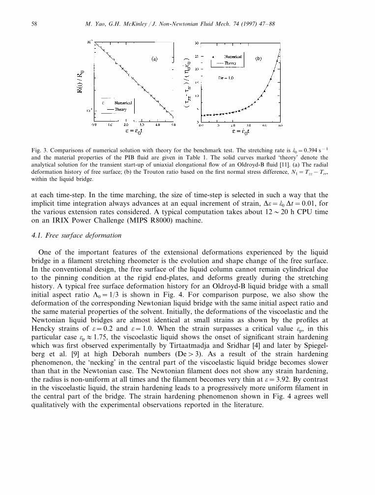
Fig. 3. Comparisons of numerical solution with theory for the benchmark test. The stretching rate is o; 0=0.394 s−1
and the material properties of the PIB fluid are given in Table 1. The solid curves marked ‘theory’ denote theanalytical solution for the transient start-up of uniaxial elongational flow of an Oldroyd-B fluid [11]. (a) The radialdeformation history of free surface; (b) the Trouton ratio based on the first normal stress difference, N1=Tzz−Trr,within the liquid bridge.
at each time-step. In the time marching, the size of time-step is selected in such a way that theimplicit time integration always advances at an equal increment of strain, Do=o; 0 Dt=0.01, forthe various extension rates considered. A typical computation takes about 12�20 h CPU timeon an IRIX Power Challenge (MIPS R8000) machine.
4.1. Free surface deformation
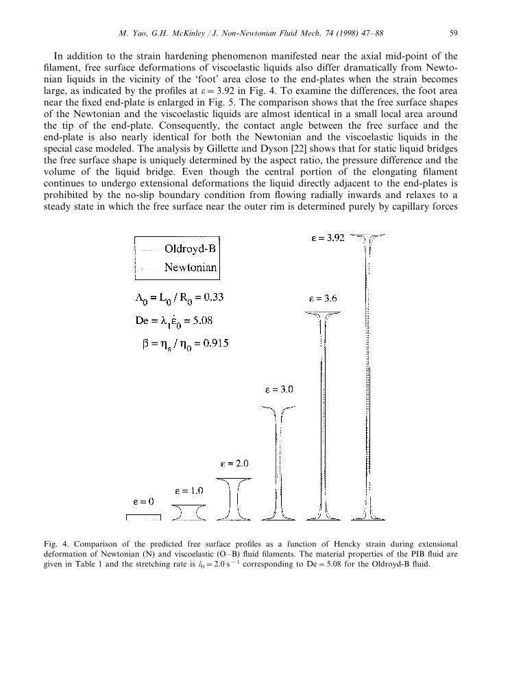
One of the important features of the extensional deformations experienced by the liquidbridge in a filament stretching rheometer is the evolution and shape change of the free surface.In the conventional design, the free surface of the liquid column cannot remain cylindrical dueto the pinning condition at the rigid end-plates, and deforms greatly during the stretchinghistory. A typical free surface deformation history for an Oldroyd-B liquid bridge with a smallinitial aspect ratio L0=1/3 is shown in Fig. 4. For comparison purpose, we also show thedeformation of the corresponding Newtonian liquid bridge with the same initial aspect ratio andthe same material properties of the solvent. Initially, the deformations of the viscoelastic and theNewtonian liquid bridges are almost identical at small strains as shown by the profiles atHencky strains of o=0.2 and o=1.0. When the strain surpasses a critical value op, in thisparticular case op:1.75, the viscoelastic liquid shows the onset of significant strain hardeningwhich was first observed experimentally by Tirtaatmadja and Sridhar [4] and later by Spiegel-berg et al. [9] at high Deborah numbers (De\3). As a result of the strain hardeningphenomenon, the ‘necking’ in the central part of the viscoelastic liquid bridge becomes slowerthan that in the Newtonian case. The Newtonian filament does not show any strain hardening,the radius is non-uniform at all times and the filament becomes very thin at o=3.92. By contrastin the viscoelastic liquid, the strain hardening leads to a progressively more uniform filament inthe central part of the bridge. The strain hardening phenomenon shown in Fig. 4 agrees wellqualitatively with the experimental observations reported in the literature.
M. Yao, G.H. McKinley / J. Non-Newtonian Fluid Mech. 74 (1998) 47–88 59
In addition to the strain hardening phenomenon manifested near the axial mid-point of thefilament, free surface deformations of viscoelastic liquids also differ dramatically from Newto-nian liquids in the vicinity of the ‘foot’ area close to the end-plates when the strain becomeslarge, as indicated by the profiles at o=3.92 in Fig. 4. To examine the differences, the foot areanear the fixed end-plate is enlarged in Fig. 5. The comparison shows that the free surface shapesof the Newtonian and the viscoelastic liquids are almost identical in a small local area aroundthe tip of the end-plate. Consequently, the contact angle between the free surface and theend-plate is also nearly identical for both the Newtonian and the viscoelastic liquids in thespecial case modeled. The analysis by Gillette and Dyson [22] shows that for static liquid bridgesthe free surface shape is uniquely determined by the aspect ratio, the pressure difference and thevolume of the liquid bridge. Even though the central portion of the elongating filamentcontinues to undergo extensional deformations the liquid directly adjacent to the end-plates isprohibited by the no-slip boundary condition from flowing radially inwards and relaxes to asteady state in which the free surface near the outer rim is determined purely by capillary forces
Fig. 4. Comparison of the predicted free surface profiles as a function of Hencky strain during extensionaldeformation of Newtonian (N) and viscoelastic (O–B) fluid filaments. The material properties of the PIB fluid aregiven in Table 1 and the stretching rate is o; 0=2.0 s−1 corresponding to De=5.08 for the Oldroyd-B fluid.
M. Yao, G.H. McKinley / J. Non-Newtonian Fluid Mech. 74 (1997) 47–8860
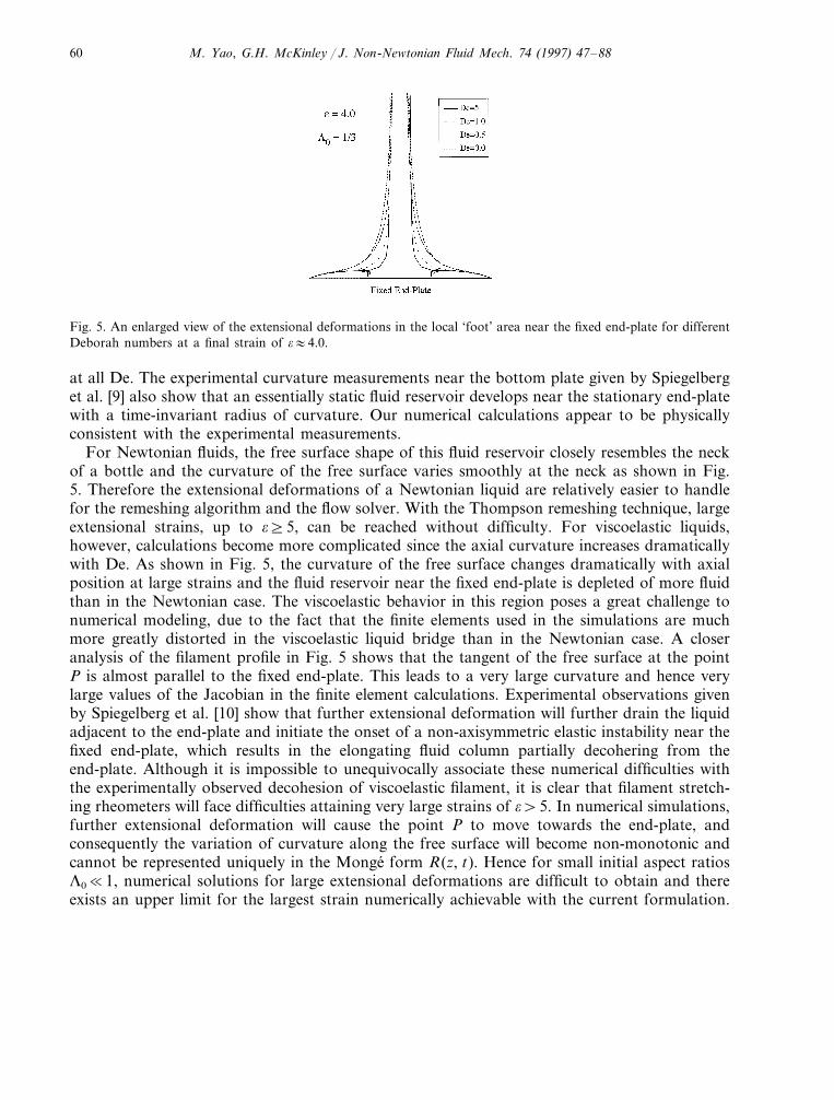
Fig. 5. An enlarged view of the extensional deformations in the local ‘foot’ area near the fixed end-plate for differentDeborah numbers at a final strain of o:4.0.
at all De. The experimental curvature measurements near the bottom plate given by Spiegelberget al. [9] also show that an essentially static fluid reservoir develops near the stationary end-platewith a time-invariant radius of curvature. Our numerical calculations appear to be physicallyconsistent with the experimental measurements.
For Newtonian fluids, the free surface shape of this fluid reservoir closely resembles the neckof a bottle and the curvature of the free surface varies smoothly at the neck as shown in Fig.5. Therefore the extensional deformations of a Newtonian liquid are relatively easier to handlefor the remeshing algorithm and the flow solver. With the Thompson remeshing technique, largeextensional strains, up to o]5, can be reached without difficulty. For viscoelastic liquids,however, calculations become more complicated since the axial curvature increases dramaticallywith De. As shown in Fig. 5, the curvature of the free surface changes dramatically with axialposition at large strains and the fluid reservoir near the fixed end-plate is depleted of more fluidthan in the Newtonian case. The viscoelastic behavior in this region poses a great challenge tonumerical modeling, due to the fact that the finite elements used in the simulations are muchmore greatly distorted in the viscoelastic liquid bridge than in the Newtonian case. A closeranalysis of the filament profile in Fig. 5 shows that the tangent of the free surface at the pointP is almost parallel to the fixed end-plate. This leads to a very large curvature and hence verylarge values of the Jacobian in the finite element calculations. Experimental observations givenby Spiegelberg et al. [10] show that further extensional deformation will further drain the liquidadjacent to the end-plate and initiate the onset of a non-axisymmetric elastic instability near thefixed end-plate, which results in the elongating fluid column partially decohering from theend-plate. Although it is impossible to unequivocally associate these numerical difficulties withthe experimentally observed decohesion of viscoelastic filament, it is clear that filament stretch-ing rheometers will face difficulties attaining very large strains of o\5. In numerical simulations,further extensional deformation will cause the point P to move towards the end-plate, andconsequently the variation of curvature along the free surface will become non-monotonic andcannot be represented uniquely in the Monge form R(z, t). Hence for small initial aspect ratiosL0�1, numerical solutions for large extensional deformations are difficult to obtain and thereexists an upper limit for the largest strain numerically achievable with the current formulation.
M. Yao, G.H. McKinley / J. Non-Newtonian Fluid Mech. 74 (1998) 47–88 61
Our computational experience shows that the upper bound for numerical accessibility to largestrains depends on several factors, including the initial aspect ratio, Deborah number, theviscosity ratio b hs/h0 and the constitutive model, etc. For the Oldroyd-B fluid model withL0=1/3, b=0.91 and De=5.1, the highest Hencky strain achievable in our computation isabout 4.0.
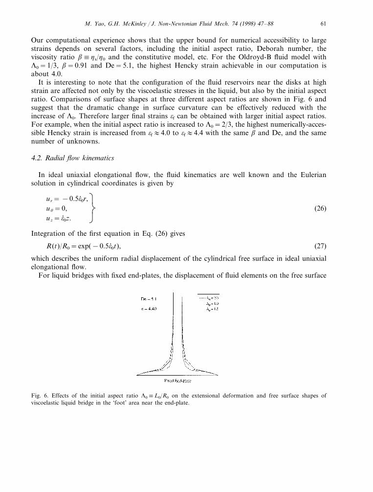
It is interesting to note that the configuration of the fluid reservoirs near the disks at highstrain are affected not only by the viscoelastic stresses in the liquid, but also by the initial aspectratio. Comparisons of surface shapes at three different aspect ratios are shown in Fig. 6 andsuggest that the dramatic change in surface curvature can be effectively reduced with theincrease of L0. Therefore larger final strains of can be obtained with larger initial aspect ratios.For example, when the initial aspect ratio is increased to L0=2/3, the highest numerically-acces-sible Hencky strain is increased from of:4.0 to of:4.4 with the same b and De, and the samenumber of unknowns.
4.2. Radial flow kinematics
In ideal uniaxial elongational flow, the fluid kinematics are well known and the Euleriansolution in cylindrical coordinates is given by
ur= −0.5o; 0r,uu=0,uz=o; 0z.
ÌÂ
Å(26)
Integration of the first equation in Eq. (26) gives
R(t)/R0=exp(−0.5o; 0t), (27)
which describes the uniform radial displacement of the cylindrical free surface in ideal uniaxialelongational flow.
For liquid bridges with fixed end-plates, the displacement of fluid elements on the free surface
Fig. 6. Effects of the initial aspect ratio L0 L0/R0 on the extensional deformation and free surface shapes ofviscoelastic liquid bridge in the ‘foot’ area near the end-plate.
M. Yao, G.H. McKinley / J. Non-Newtonian Fluid Mech. 74 (1997) 47–8862
(as well as within the entire domain) is temporally and spatially non-homogeneous. The radialmovement at the two ends of the liquid bridge is completely restrained due to the pinningconditions at the fixed end-plates. As a result, the decrease of the radius at the central part ofthe filament is much faster than in ideal uniaxial elongational flow so that the volume of thebridge is conserved. Consequently, the flow kinematics in the liquid bridges with fixed end-platesis much more complicated and deviates significantly from the flow field given in Eq. (26). Thepresence of a deforming free surface whose position is unknown a priori means that exactanalytical solutions for the velocity field are not available for either the Newtonian andviscoelastic liquid bridge problems, and the flow field in general can only be computednumerically.
However, an approximate analytical solution has been obtained for the initial response of aNewtonian liquid bridge based on lubrication theory [9]. This solution is valid for small aspectratios (L0�1) and viscous liquid filaments (Re�1) at short times when the free surface isapproximately cylindrical. This lubrication theory solution is very similar to that in the classicalsqueeze film problem of Stefan [11,23]. The major difference is that the direction of motion isreversed in the liquid bridge case and the boundary motion increases exponentially in time. Theaxial and radial velocity components of the lubrication theory solution are described by thefollowing simple expressions in dimensional form
ur= −3o; 0r�
1−z
Lp
� zLp
, uz=L: p�
3−2z
Lp
�� zLp
�2
, (28)
which satisfies the velocity boundary conditions at the two end-plates, but does not satisfy thestress boundary conditions on the free surface. However, since the Capillary number Ca�1 inmost tests this error is small. Although Eq. (28) is derived for Newtonian liquids, it should alsobe a good approximation for Oldroyd-B liquid bridges at small strains based on the squeeze flowexperiment and calculations by Phen-Thien and Boger [24,25]. In addition, experimentalobservations in filament stretching devices [9] also show that the fluid response is Newtonian foroB1. Setting z=Lp/2 in Eq. (28) and integrating ur suggest that the mid-point of fluid filamentshould initially decrease as
Rmid(t)/R0=exp(−0.75o; 0t). (29)
By substituting Eq. (28) into Eq. (10), we obtain the following expression for the rate ofdeformation tensor
Dzz=6o; 0�
1−z
Lp
� zLp
, Drz= −3o; 0�
1−2z
Lp
� rLp
. (30)
The lubrication solution predicts that Dzz is parabolic in the axial direction with a maximumvalue at z/Lp=0.5 of
Dzz=1.5o; 0. (31)
The results in Eqs. (29) and (31) suggest that at the very beginning of the deformation the fluidelement at the mid-point section experiences a local extensional strain rate which is about 50%higher than the imposed global strain rate o; 0; however the average of Dzz along the axialdirection is still the same as the imposed o; 0.
M. Yao, G.H. McKinley / J. Non-Newtonian Fluid Mech. 74 (1998) 47–88 63
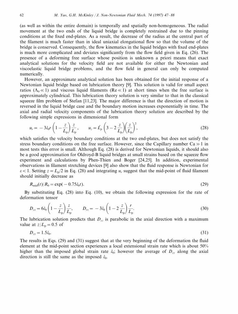
Fig. 7. Variation of the minimum radius of the liquid column, Rmin, with respect to the imposed axial Hencky strain,o=o; 0t, and as a function of Deborah number. De=0 is the corresponding Newtonian case. The geometrical andmaterial parameters for the PIB fluid used are the same as given in Table 1.
To quantify the extensional deformation at the central part of the filament, we show thecomputed time history of the minimum radius, Rmin(t) as a function of Hencky strain in Fig. 7.The lubrication prediction in Eq. (29) is in good agreement with the computed rate of decreaseobserved in the Newtonian filament at all strains up to o=2.5 as shown by the zero De curvein Fig. 7. For larger strains o\2.5, the necking in Rmin accelerates slightly and eventually leadsto a capillary instability in the vicinity of the mid-plane of the Newtonian liquid bridge. Forviscoelastic filaments, there are in general two distinct regions in the curve of Rmin(t). In the firstregion, corresponding to strains oB1.75, the evolution in Rmin is the same as Newtonian and thefilament undergoes significant necking as observed in Fig. 4. This result agrees well with theconclusions made in the literature [24,25] that the initial behavior of the Oldroyd-B fluid duringsqueeze flow is basically that of the Newtonian solvent contribution. The second region forstrains o\1.75 is characterized by a slope change in the curve of Rmin(t). In this region theradius decreases more slowly than that in the ideal uniaxial elongational flow due to strainhardening in the fluid. This characteristic change in the slope shown in Fig. 7 agrees well withthe experimental measurements shown in [2,3,7,9].
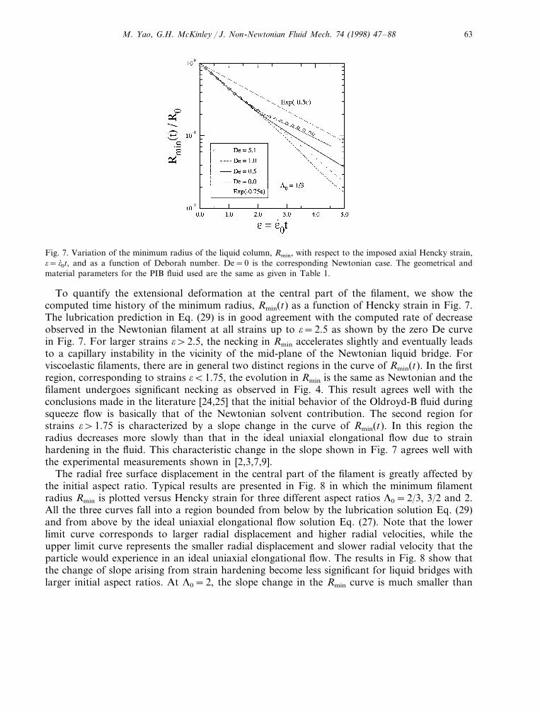
The radial free surface displacement in the central part of the filament is greatly affected bythe initial aspect ratio. Typical results are presented in Fig. 8 in which the minimum filamentradius Rmin is plotted versus Hencky strain for three different aspect ratios L0=2/3, 3/2 and 2.All the three curves fall into a region bounded from below by the lubrication solution Eq. (29)and from above by the ideal uniaxial elongational flow solution Eq. (27). Note that the lowerlimit curve corresponds to larger radial displacement and higher radial velocities, while theupper limit curve represents the smaller radial displacement and slower radial velocity that theparticle would experience in an ideal uniaxial elongational flow. The results in Fig. 8 show thatthe change of slope arising from strain hardening become less significant for liquid bridges withlarger initial aspect ratios. At L0=2, the slope change in the Rmin curve is much smaller than
M. Yao, G.H. McKinley / J. Non-Newtonian Fluid Mech. 74 (1997) 47–8864
that for L0=2/3, and the radial deformation is much closer to the ideal curve R(t)/R0=exp(−0.5o). The trend indicated in Fig. 8 provides useful information for design of future experiments,namely a more effective design strategy is to choose larger initial ratios of the liquid filament.
The lubrication solution given in Eq. (28) predicts that the axial velocity is a cubic functionof z and the radial velocity is a parabolic function of z, whereas the ideal uniaxial elongationalflow described by Eq. (26) has a linear variation in z for uz and a constant value for ur.Comparisons of the numerical simulation for the Newtonian and Oldroyd-B fluids with thesepredictions are presented in Figs. 9 and 10. The axial velocity profile along the centerline r=0and the radial velocity profile on the deformed free surface (r=R(z, t)) respectively are plottedover a range of strain levels.
In general, the flow in the liquid bridge differs from the ideal uniaxial elongational flow,except in the immediate vicinity of the mid-point section z=Lp/2 where the agreement is purelya result of geometric symmetry. For the Newtonian liquid, the lubrication solution provides asurprisingly good approximation for uz up to o:2.0, and the agreement is still fairly good evenfor larger strains up to o=3.8, as shown in Fig. 9. For Oldroyd-B fluid, the lubrication solutionof uz is a very good approximation for o51.0. For o\1.0, the flow behavior of the Oldroyd-Bmodel starts to deviate gradually from that of Newtonian liquid, and the lubrication predictionbecomes increasingly invalid.
The change in the deformation characteristics documented in Figs. 7 and 8 for the viscoelasticfilaments is also manifested in Figs. 9 and 10. At strain levels o\2.0, the axial velocity near bothend-plates dramatically changes. The velocity gradient (uz/(z at the mid-plane (z/Lp=0.5)decreases below both the lubrication solution and the ideal homogeneous uniaxial elongationdue to the onset of strain-hardening. By contrast, near the end-plates (z/Lp=0, 1), the axialvelocity gradient dramatically increases indicating that fluid is progressively drained out of the‘foot’ or reservoir region.
Fig. 8. Effects of the initial aspect ratio on the radial deformation of the viscoelastic liquid bridge as a function ofthe imposed global Hencky strain, o.
M. Yao, G.H. McKinley / J. Non-Newtonian Fluid Mech. 74 (1998) 47–88 65
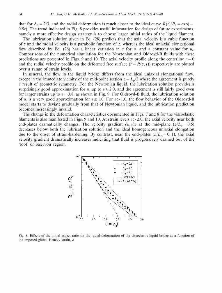
Fig. 9. Profiles of the axial velocity along the centerline of the liquid bridge at four typical strain levels. Numericalsolutions of the Oldroyd-B and the Newtonian liquids are compared with the ideal uniaxial elongational flow (dotcurves) and the lubrication solution given by Eq. (28) (solid curves). The same initial aspect ratio L0=1/3 andextension rate o; 0=2 s−1 were used for both the Newtonian and viscoelastic cases which leads to De=5.08 for thelatter simulation.
Comparisons with numerical simulations also indicate that the lubrication solution providesan accurate description of the radial velocity profile along the free surface, at least at smallstrains, as shown in Fig. 10. In the uniaxial elongational flow, ur is homogeneous in space, bycontrast in the filament stretching devices, ur is non-homogeneous due to the boundaryconditions imposed by the end-plates. For viscous Newtonian liquids with material propertiestypified by those in Table 1, the lubrication solution appears to be a fairly good approximationeven at large strains up to o=3.8 except very close to the pinned contact regions. Here thevelocity gradient (ur/(z decreases to zero confirming that the region becomes quasi-static. Forthe Oldroyd-B fluid, the radial velocity of the free surface gradually decreases at strains o\1.75and becomes increasingly axially uniform in the central part of the domain. For o]3.0, the
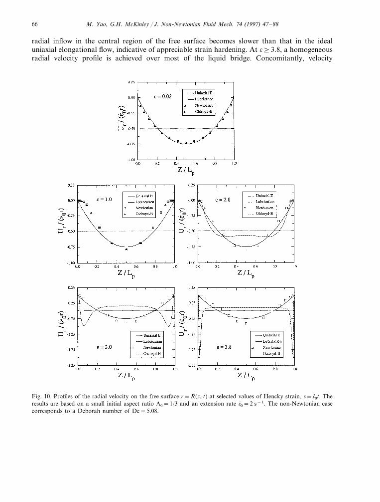
M. Yao, G.H. McKinley / J. Non-Newtonian Fluid Mech. 74 (1997) 47–8866
radial inflow in the central region of the free surface becomes slower than that in the idealuniaxial elongational flow, indicative of appreciable strain hardening. At o]3.8, a homogeneousradial velocity profile is achieved over most of the liquid bridge. Concomitantly, velocity
Fig. 10. Profiles of the radial velocity on the free surface r=R(z, t) at selected values of Hencky strain, o=o; 0t. Theresults are based on a small initial aspect ratio L0=1/3 and an extension rate o; 0=2 s−1. The non-Newtonian casecorresponds to a Deborah number of De=5.08.
M. Yao, G.H. McKinley / J. Non-Newtonian Fluid Mech. 74 (1998) 47–88 67
boundary layers develop near the two end-plates at high strains. These velocity boundary layersfurther contribute to the dramatic difference between viscoelastic and Newtonian liquids in freesurface shapes near the foot area as discussed above in Section 4.1. Resolution of theseboundary layers contributes to the difficulties in attaining high strains numerically.
4.3. Rate of deformation
The deformation history of the liquid bridge can also be quantitatively characterized by theextensional and shear strain rates which represents the deformation rate that the fluid elementsexperience during the stretching process. The spatial and temporal variations of strain rates canbe used in error control for quantifying inhomogeneities and deviations of the real flow fieldfrom the ideal uniaxial elongational flow. Ideally, we would like to control the actual strain rateto be purely extensional, homogeneous and identical to the imposed value of o; 0. However, as wehave shown, the actual strain rate is not that expected in a simple extensional flow and, ingeneral, it varies both spatially and temporally. Since direct measurement of the detaileddistribution of strain rate within the liquid bridge is very difficult, numerical simulation plays animportant role in studying the rate of deformation and provides some interesting insight into theflow field.
For the cylindrical coordinate system shown in Fig. 1, the rate of deformation tensor Ddefined in Eq. (10) has four independent non-zero components: Drr, Drz, Dzz and Duu, all ofwhich vary with spatial position and time. Among them, the components Dzz and Drz are ofmost interest to our study since they characterize the extension rate and the shear rate in thefluid. For a homogeneous uniaxial elongational flow given by Eq. (26), Dzz o; 0 and Drz 0.When the end-plate diameter is fixed as in conventional stretching devices, the flow field isaltered by the pinning conditions at the rigid end-plates, as a result, Dzz becomes a function oftime and space. It is interesting to note the value of D at the rigid end-plates. For incompressiblefluids, it is easy to prove from the no-slip boundary condition and the continuity equation that
Drr=Dzz 0. Ö{(r, z)�z=0 or z=Lp}. (32)
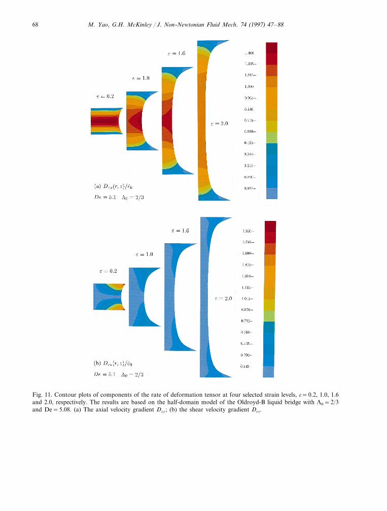
Boundary layers in the velocity gradients (and associated stresses) thus develop near the rigidfixtures. For the Oldroyd-B fluid, typical spatial and temporal variations of Dzz and Drz areshown in the contours plots presented in Fig. 11. The actual extensional strain rate within theliquid bridge is highly non-homogeneous at the initial stage of stretching as seen from thecontours plots of o=0.2 and 1.0 in Fig. 11(a). At o=0.2, the contours are almost parabolicallydistributed in the axial direction and radially uniform as expected from Eq. (30). However, thenon-homogeneity is gradually reduced with increasing strain and a homogeneous deformationzone (HDZ) is formed at the central part of the domain as shown by the plot of o=2 in Fig.11(a). Our simulation shows that this HDZ continues to expand towards the two end-plates withfurther stretching and strain-hardening in the fluid. The contour plot of Drz at o=0.2 in Fig.11(b) suggests that a significant shearing component is generated between the plates at smallstrains. As shown in Fig. 11(b), the shear rate is negligibly small in the central part of the liquidbridge but is largest near the pinned free surface. Subsequent contour plots in Fig. 11(b) indicatethat the shear rate decays rapidly with the increase of strain.
As we have shown in Fig. 9, the lubrication prediction (derived in the limit L0�1) remainsa good approximation even up to strains of o�1.75 for both the Newtonian and Oldroyd-B
M. Yao, G.H. McKinley / J. Non-Newtonian Fluid Mech. 74 (1997) 47–8868
Fig. 11. Contour plots of components of the rate of deformation tensor at four selected strain levels, o=0.2, 1.0, 1.6and 2.0, respectively. The results are based on the half-domain model of the Oldroyd-B liquid bridge with L0=2/3and De=5.08. (a) The axial velocity gradient Dzz ; (b) the shear velocity gradient Drz.
M. Yao, G.H. McKinley / J. Non-Newtonian Fluid Mech. 74 (1998) 47–88 69
fluids. Beyond this range, the extensional behaviors of the two liquids become significantlydifferent. For Newtonian filaments within a strain range 1.5BoB4, the extensional strain rateat the mid-point section tends to increase slightly with strain due to the increasing capillarypressure and the maximum axial velocity gradient Dzz remains at the mid-plane of the filamentwhere the radius is smallest. For Newtonian liquid bridges, there is no strain hardening and thenecking is always largest at the mid-plane between the two end-plates. Consequently, althoughwe do not resolve the dynamics of the actual filament breakup process, our numerical modelingindicates that the Newtonian liquid bridges in conventional filament stretching devices will breakin the middle, which agrees well with experimental observations. For the viscoelastic fluid, strainhardening becomes important at large strains and strain rates due to the elongation of thepolymer chains. As a result, the extensional strain rate in the central part of liquid bridgedecreases gradually and two boundary layers in Dzz are simultaneously developed near the twoend-plates as indicated by the plots of o=3 and 3.8 in Fig. 9. Physically, the strain-hardeningliquid in the middle of the column becomes increasingly difficult to stretch, and it becomesrelatively easier to pull the unstretched material out of the fluid reservoir in the ‘foot’ areasadjacent to the two end-plates. With the development of the two boundary layers, theextensional strain rate is increased rapidly near the two end-plates. At o=3.8, the maximumvalues of Dzz are about 4.5 times larger than the imposed global extensional rate o; 0 and continueto increase dramatically with further stretching. The break-up mechanism in viscoelastic liquidbridge at high De is thus anticipated to be quite different from the Newtonian case. The strainhardening and viscoelastic behavior of the fluid prevent the filament from breaking in themiddle. Instead, the increasingly rapid rate of liquid drainage from the ‘foot’ regions leads to auniform elastic column connected by a thin fluid film to the rigid end-plate. Numericalcalculations show that the radius of curvature in these regions becomes very small and large(negative) pressure gradients develop as the filament elongates. Ultimately the slope #R/#z of thefree surface becomes almost zero near the end-plates and numerical convergence is lost.Although we do not directly simulate the elastic instability, this sequence appears to beconsistent with recent experimental observations of elastic filament break-up and decohesion[10].
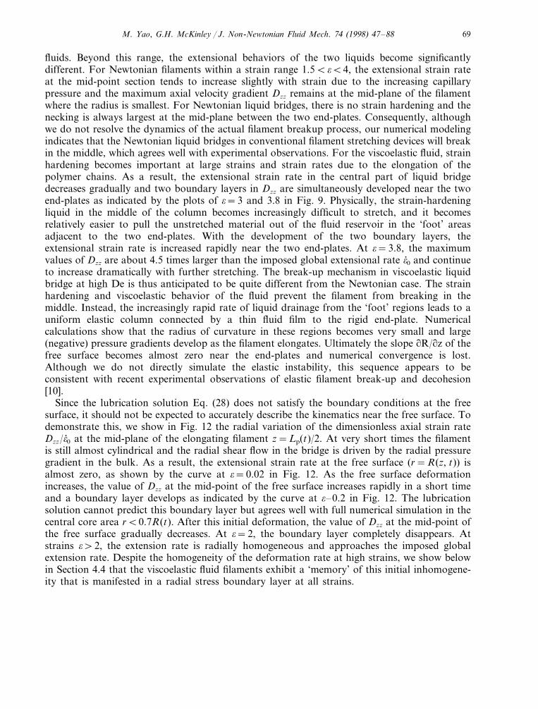
Since the lubrication solution Eq. (28) does not satisfy the boundary conditions at the freesurface, it should not be expected to accurately describe the kinematics near the free surface. Todemonstrate this, we show in Fig. 12 the radial variation of the dimensionless axial strain rateDzz/o; 0 at the mid-plane of the elongating filament z=Lp(t)/2. At very short times the filamentis still almost cylindrical and the radial shear flow in the bridge is driven by the radial pressuregradient in the bulk. As a result, the extensional strain rate at the free surface (r=R(z, t)) isalmost zero, as shown by the curve at o=0.02 in Fig. 12. As the free surface deformationincreases, the value of Dzz at the mid-point of the free surface increases rapidly in a short timeand a boundary layer develops as indicated by the curve at o–0.2 in Fig. 12. The lubricationsolution cannot predict this boundary layer but agrees well with full numerical simulation in thecentral core area rB0.7R(t). After this initial deformation, the value of Dzz at the mid-point ofthe free surface gradually decreases. At o=2, the boundary layer completely disappears. Atstrains o\2, the extension rate is radially homogeneous and approaches the imposed globalextension rate. Despite the homogeneity of the deformation rate at high strains, we show belowin Section 4.4 that the viscoelastic fluid filaments exhibit a ‘memory’ of this initial inhomogene-ity that is manifested in a radial stress boundary layer at all strains.
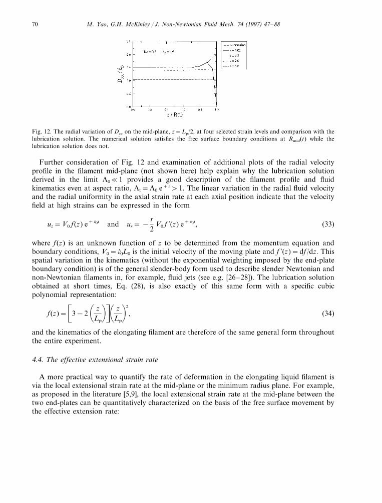
M. Yao, G.H. McKinley / J. Non-Newtonian Fluid Mech. 74 (1997) 47–8870
Fig. 12. The radial variation of Dzz on the mid-plane, z=Lp/2, at four selected strain levels and comparison with thelubrication solution. The numerical solution satisfies the free surface boundary conditions at Rmid(t) while thelubrication solution does not.
Further consideration of Fig. 12 and examination of additional plots of the radial velocityprofile in the filament mid-plane (not shown here) help explain why the lubrication solutionderived in the limit L0�1 provides a good description of the filament profile and fluidkinematics even at aspect ratio, Lt=L0 e+o\1. The linear variation in the radial fluid velocityand the radial uniformity in the axial strain rate at each axial position indicate that the velocityfield at high strains can be expressed in the form
uz=V0 f(z) e+o; 0t and ur= −r2
V0 f %(z) e+o; 0t, (33)
where f(z) is an unknown function of z to be determined from the momentum equation andboundary conditions, V0=o; 0L0 is the initial velocity of the moving plate and f %(z)=df/dz. Thisspatial variation in the kinematics (without the exponential weighting imposed by the end-plateboundary condition) is of the general slender-body form used to describe slender Newtonian andnon-Newtonian filaments in, for example, fluid jets (see e.g. [26–28]). The lubrication solutionobtained at short times, Eq. (28), is also exactly of this same form with a specific cubicpolynomial representation:
f(z)=�
3−2� z
Lp
�n� zLp
�2
, (34)
and the kinematics of the elongating filament are therefore of the same general form throughoutthe entire experiment.
4.4. The effecti6e extensional strain rate
A more practical way to quantify the rate of deformation in the elongating liquid filament isvia the local extensional strain rate at the mid-plane or the minimum radius plane. For example,as proposed in the literature [5,9], the local extensional strain rate at the mid-plane between thetwo end-plates can be quantitatively characterized on the basis of the free surface movement bythe effective extension rate:
M. Yao, G.H. McKinley / J. Non-Newtonian Fluid Mech. 74 (1998) 47–88 71
o; eff −2d(ln Rmid)/dt= −2Ur,mid/Rmid, (35)
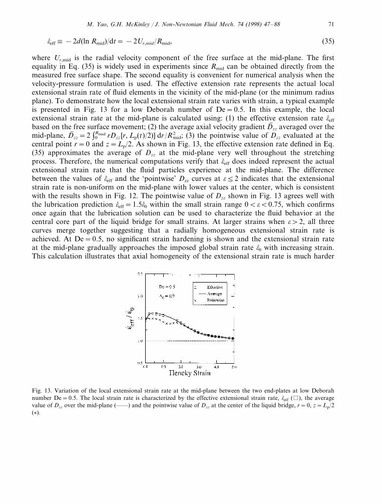
where Ur,mid is the radial velocity component of the free surface at the mid-plane. The firstequality in Eq. (35) is widely used in experiments since Rmid can be obtained directly from themeasured free surface shape. The second equality is convenient for numerical analysis when thevelocity-pressure formulation is used. The effective extension rate represents the actual localextensional strain rate of fluid elements in the vicinity of the mid-plane (or the minimum radiusplane). To demonstrate how the local extensional strain rate varies with strain, a typical exampleis presented in Fig. 13 for a low Deborah number of De=0.5. In this example, the localextensional strain rate at the mid-plane is calculated using: (1) the effective extension rate o; eff
based on the free surface movement; (2) the average axial velocity gradient D( zz averaged over themid-plane, D( zz=2 Rmid
0 rDzz [r, Lp(t)/2)] dr/R2mid; (3) the pointwise value of Dzz evaluated at the
central point r=0 and z=Lp/2. As shown in Fig. 13, the effective extension rate defined in Eq.(35) approximates the average of Dzz at the mid-plane very well throughout the stretchingprocess. Therefore, the numerical computations verify that o; eff does indeed represent the actualextensional strain rate that the fluid particles experience at the mid-plane. The differencebetween the values of o; eff and the ‘pointwise’ Dzz curves at o52 indicates that the extensionalstrain rate is non-uniform on the mid-plane with lower values at the center, which is consistentwith the results shown in Fig. 12. The pointwise value of Dzz shown in Fig. 13 agrees well withthe lubrication prediction o; eff=1.5o; 0 within the small strain range 0BoB0.75, which confirmsonce again that the lubrication solution can be used to characterize the fluid behavior at thecentral core part of the liquid bridge for small strains. At larger strains when o\2, all threecurves merge together suggesting that a radially homogeneous extensional strain rate isachieved. At De=0.5, no significant strain hardening is shown and the extensional strain rateat the mid-plane gradually approaches the imposed global strain rate o; 0 with increasing strain.This calculation illustrates that axial homogeneity of the extensional strain rate is much harder
Fig. 13. Variation of the local extensional strain rate at the mid-plane between the two end-plates at low Deborahnumber De=0.5. The local strain rate is characterized by the effective extensional strain rate, o; eff ( ), the averagevalue of Dzz over the mid-plane (——) and the pointwise value of Dzz at the center of the liquid bridge, r=0, z=Lp/2(�).
M. Yao, G.H. McKinley / J. Non-Newtonian Fluid Mech. 74 (1997) 47–8872
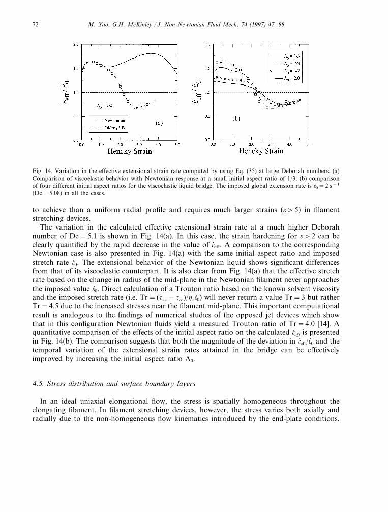
Fig. 14. Variation in the effective extensional strain rate computed by using Eq. (35) at large Deborah numbers. (a)Comparison of viscoelastic behavior with Newtonian response at a small initial aspect ratio of 1/3; (b) comparisonof four different initial aspect ratios for the viscoelastic liquid bridge. The imposed global extension rate is o; 0=2 s−1
(De=5.08) in all the cases.
to achieve than a uniform radial profile and requires much larger strains (o\5) in filamentstretching devices.
The variation in the calculated effective extensional strain rate at a much higher Deborahnumber of De=5.1 is shown in Fig. 14(a). In this case, the strain hardening for o\2 can beclearly quantified by the rapid decrease in the value of o; eff. A comparison to the correspondingNewtonian case is also presented in Fig. 14(a) with the same initial aspect ratio and imposedstretch rate o; 0. The extensional behavior of the Newtonian liquid shows significant differencesfrom that of its viscoelastic counterpart. It is also clear from Fig. 14(a) that the effective stretchrate based on the change in radius of the mid-plane in the Newtonian filament never approachesthe imposed value o; 0. Direct calculation of a Trouton ratio based on the known solvent viscosityand the imposed stretch rate (i.e. Tr= (tzz−trr)/hso; 0) will never return a value Tr=3 but ratherTr=4.5 due to the increased stresses near the filament mid-plane. This important computationalresult is analogous to the findings of numerical studies of the opposed jet devices which showthat in this configuration Newtonian fluids yield a measured Trouton ratio of Tr=4.0 [14]. Aquantitative comparison of the effects of the initial aspect ratio on the calculated o; eff is presentedin Fig. 14(b). The comparison suggests that both the magnitude of the deviation in o; eff/o; 0 and thetemporal variation of the extensional strain rates attained in the bridge can be effectivelyimproved by increasing the initial aspect ratio L0.
4.5. Stress distribution and surface boundary layers
In an ideal uniaxial elongational flow, the stress is spatially homogeneous throughout theelongating filament. In filament stretching devices, however, the stress varies both axially andradially due to the non-homogeneous flow kinematics introduced by the end-plate conditions.
M. Yao, G.H. McKinley / J. Non-Newtonian Fluid Mech. 74 (1998) 47–88 73
Numerical simulations can provide detailed information about stress distributions within theliquid. These detailed stress distributions are in general not available from direct measurements.
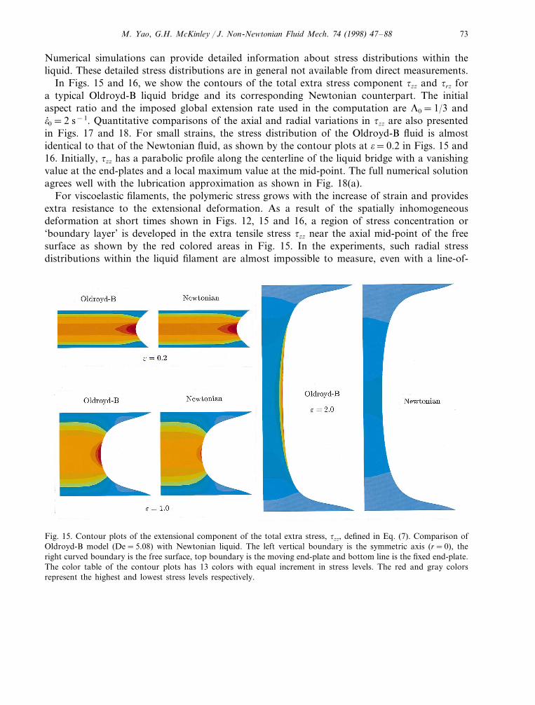
In Figs. 15 and 16, we show the contours of the total extra stress component tzz and trz fora typical Oldroyd-B liquid bridge and its corresponding Newtonian counterpart. The initialaspect ratio and the imposed global extension rate used in the computation are L0=1/3 ando; 0=2 s−1. Quantitative comparisons of the axial and radial variations in tzz are also presentedin Figs. 17 and 18. For small strains, the stress distribution of the Oldroyd-B fluid is almostidentical to that of the Newtonian fluid, as shown by the contour plots at o=0.2 in Figs. 15 and16. Initially, tzz has a parabolic profile along the centerline of the liquid bridge with a vanishingvalue at the end-plates and a local maximum value at the mid-point. The full numerical solutionagrees well with the lubrication approximation as shown in Fig. 18(a).
For viscoelastic filaments, the polymeric stress grows with the increase of strain and providesextra resistance to the extensional deformation. As a result of the spatially inhomogeneousdeformation at short times shown in Figs. 12, 15 and 16, a region of stress concentration or‘boundary layer’ is developed in the extra tensile stress tzz near the axial mid-point of the freesurface as shown by the red colored areas in Fig. 15. In the experiments, such radial stressdistributions within the liquid filament are almost impossible to measure, even with a line-of-
Fig. 15. Contour plots of the extensional component of the total extra stress, tzz, defined in Eq. (7). Comparison ofOldroyd-B model (De=5.08) with Newtonian liquid. The left vertical boundary is the symmetric axis (r=0), theright curved boundary is the free surface, top boundary is the moving end-plate and bottom line is the fixed end-plate.The color table of the contour plots has 13 colors with equal increment in stress levels. The red and gray colorsrepresent the highest and lowest stress levels respectively.
M. Yao, G.H. McKinley / J. Non-Newtonian Fluid Mech. 74 (1997) 47–8874
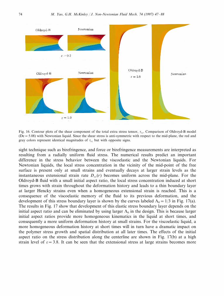
Fig. 16. Contour plots of the shear component of the total extra stress tensor, trz. Comparison of Oldroyd-B model(De=5.08) with Newtonian liquid. Since the shear stress is anti-symmetric with respect to the mid-plane, the red andgray colors represent identical magnitudes of trz but with opposite signs.
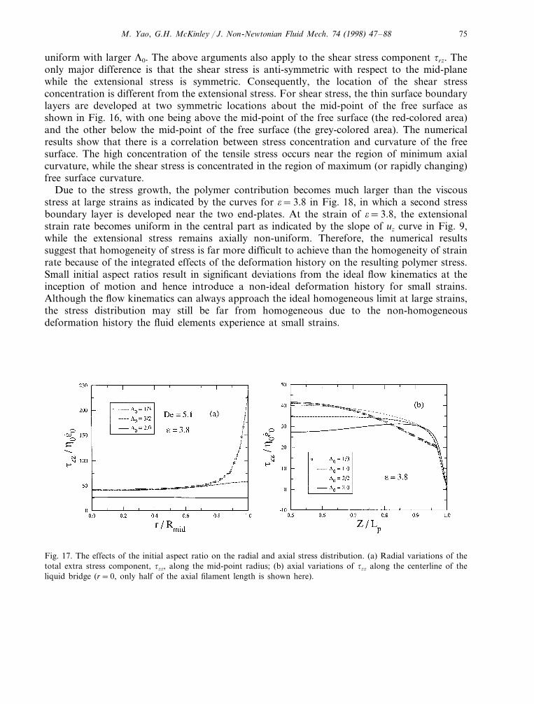
sight technique such as birefringence, and force or birefringence measurements are interpreted asresulting from a radially uniform fluid stress. The numerical results predict an importantdifference in the stress behavior between the viscoelastic and the Newtonian liquids. ForNewtonian liquids, the local stress concentration in the vicinity of the mid-point of the freesurface is present only at small strains and eventually decays at larger strain levels as theinstantaneous extensional strain rate Dzz(r) becomes uniform across the mid-plane. For theOldroyd-B fluid with a small initial aspect ratio, the local stress concentration induced at shorttimes grows with strain throughout the deformation history and leads to a thin boundary layerat larger Hencky strains even when a homogeneous extensional strain is reached. This is aconsequence of the viscoelastic memory of the fluid to its previous deformation, and thedevelopment of this stress boundary layer is shown by the curves labeled L0=1/3 in Fig. 17(a).The results in Fig. 17 show that development of this elastic stress boundary layer depends on theinitial aspect ratio and can be eliminated by using larger L0 in the design. This is because largerinitial aspect ratios provide more homogeneous kinematics in the liquid at short times, andconsequently a more uniform deformation history at small strains. For the viscoelastic liquid, amore homogeneous deformation history at short times will in turn have a dramatic impact onthe polymer stress growth and spatial distribution at all later times. The effects of the initialaspect ratio on the stress distribution along the centerline are shown in Fig. 17(b) at a highstrain level of o=3.8. It can be seen that the extensional stress at large strains becomes more
M. Yao, G.H. McKinley / J. Non-Newtonian Fluid Mech. 74 (1998) 47–88 75
uniform with larger L0. The above arguments also apply to the shear stress component trz. Theonly major difference is that the shear stress is anti-symmetric with respect to the mid-planewhile the extensional stress is symmetric. Consequently, the location of the shear stressconcentration is different from the extensional stress. For shear stress, the thin surface boundarylayers are developed at two symmetric locations about the mid-point of the free surface asshown in Fig. 16, with one being above the mid-point of the free surface (the red-colored area)and the other below the mid-point of the free surface (the grey-colored area). The numericalresults show that there is a correlation between stress concentration and curvature of the freesurface. The high concentration of the tensile stress occurs near the region of minimum axialcurvature, while the shear stress is concentrated in the region of maximum (or rapidly changing)free surface curvature.
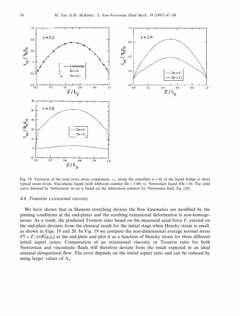
Due to the stress growth, the polymer contribution becomes much larger than the viscousstress at large strains as indicated by the curves for o=3.8 in Fig. 18, in which a second stressboundary layer is developed near the two end-plates. At the strain of o=3.8, the extensionalstrain rate becomes uniform in the central part as indicated by the slope of uz curve in Fig. 9,while the extensional stress remains axially non-uniform. Therefore, the numerical resultssuggest that homogeneity of stress is far more difficult to achieve than the homogeneity of strainrate because of the integrated effects of the deformation history on the resulting polymer stress.Small initial aspect ratios result in significant deviations from the ideal flow kinematics at theinception of motion and hence introduce a non-ideal deformation history for small strains.Although the flow kinematics can always approach the ideal homogeneous limit at large strains,the stress distribution may still be far from homogeneous due to the non-homogeneousdeformation history the fluid elements experience at small strains.
Fig. 17. The effects of the initial aspect ratio on the radial and axial stress distribution. (a) Radial variations of thetotal extra stress component, tzz, along the mid-point radius; (b) axial variations of tzz along the centerline of theliquid bridge (r=0, only half of the axial filament length is shown here).
M. Yao, G.H. McKinley / J. Non-Newtonian Fluid Mech. 74 (1997) 47–8876
Fig. 18. Variation of the total extra stress component, tzz, along the centerline (r=0) of the liquid bridge at threetypical strain levels. Viscoelastic liquid (with Deborah number De=5.08) vs. Newtonian liquid (De=0). The solidcurve denoted by ‘lubrication’ in (a) is based on the lubrication solution for Newtonian fluid, Eq. (28).
4.6. Transient extensional 6iscosity
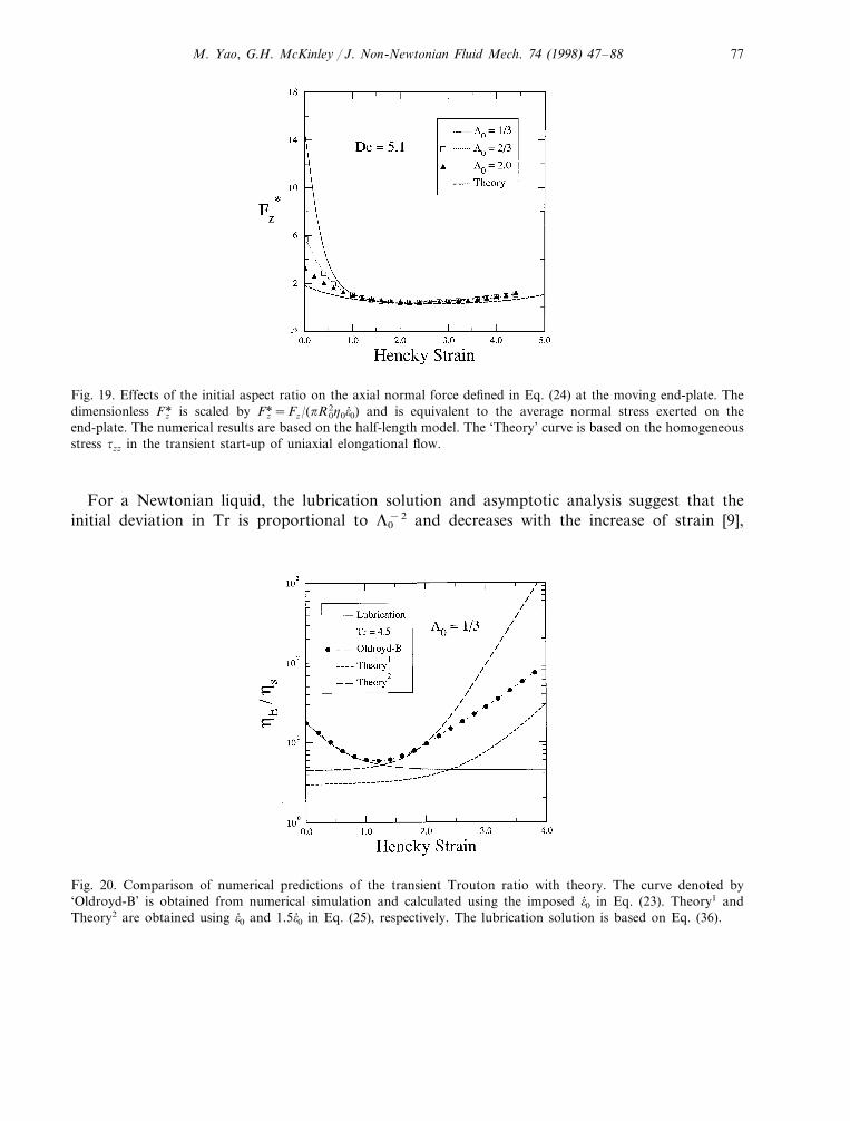
We have shown that in filament stretching devices the flow kinematics are modified by thepinning conditions at the end-plates and the resulting extensional deformation is non-homoge-neous. As a result, the predicted Trouton ratio based on the measured axial force Fz exerted onthe end-plate deviates from the classical result for the initial stage when Hencky strain is small,as shown in Figs. 19 and 20. In Fig. 19 we compute the non-dimensional average normal stressFz*=Fz/(pR2
0h0o; 0) at the end-plate and plot it as a function of Hencky strain for three differentinitial aspect ratios. Computation of an extensional viscosity or Trouton ratio for bothNewtonian and viscoelastic fluids will therefore deviate from the result expected in an idealuniaxial elongational flow. The error depends on the initial aspect ratio and can be reduced byusing larger values of L0.
M. Yao, G.H. McKinley / J. Non-Newtonian Fluid Mech. 74 (1998) 47–88 77
Fig. 19. Effects of the initial aspect ratio on the axial normal force defined in Eq. (24) at the moving end-plate. Thedimensionless Fz* is scaled by Fz*=Fz/(pR2
0h0o; 0) and is equivalent to the average normal stress exerted on theend-plate. The numerical results are based on the half-length model. The ‘Theory’ curve is based on the homogeneousstress tzz in the transient start-up of uniaxial elongational flow.
For a Newtonian liquid, the lubrication solution and asymptotic analysis suggest that theinitial deviation in Tr is proportional to L0
−2 and decreases with the increase of strain [9],
Fig. 20. Comparison of numerical predictions of the transient Trouton ratio with theory. The curve denoted by‘Oldroyd-B’ is obtained from numerical simulation and calculated using the imposed o; 0 in Eq. (23). Theory1 andTheory2 are obtained using o; 0 and 1.5o; 0 in Eq. (25), respectively. The lubrication solution is based on Eq. (36).
M. Yao, G.H. McKinley / J. Non-Newtonian Fluid Mech. 74 (1997) 47–8878
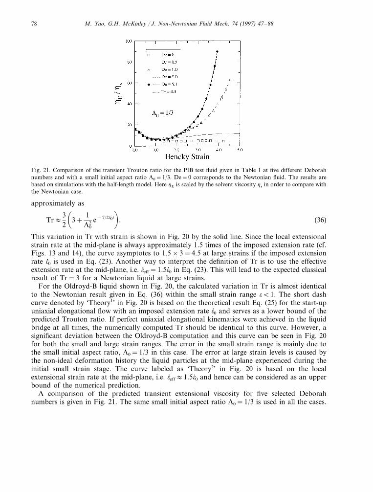
Fig. 21. Comparison of the transient Trouton ratio for the PIB test fluid given in Table 1 at five different Deborahnumbers and with a small initial aspect ratio L0=1/3. De=0 corresponds to the Newtonian fluid. The results arebased on simulations with the half-length model. Here hE is scaled by the solvent viscosity hs in order to compare withthe Newtonian case.
approximately as
Tr:32�
3+1L2
0e−7/2o; 0t�. (36)
This variation in Tr with strain is shown in Fig. 20 by the solid line. Since the local extensionalstrain rate at the mid-plane is always approximately 1.5 times of the imposed extension rate (cf.Figs. 13 and 14), the curve asymptotes to 1.5×3=4.5 at large strains if the imposed extensionrate o; 0 is used in Eq. (23). Another way to interpret the definition of Tr is to use the effectiveextension rate at the mid-plane, i.e. o; eff=1.5o; 0 in Eq. (23). This will lead to the expected classicalresult of Tr=3 for a Newtonian liquid at large strains.
For the Oldroyd-B liquid shown in Fig. 20, the calculated variation in Tr is almost identicalto the Newtonian result given in Eq. (36) within the small strain range oB1. The short dashcurve denoted by ‘Theory1’ in Fig. 20 is based on the theoretical result Eq. (25) for the start-upuniaxial elongational flow with an imposed extension rate o; 0 and serves as a lower bound of thepredicted Trouton ratio. If perfect uniaxial elongational kinematics were achieved in the liquidbridge at all times, the numerically computed Tr should be identical to this curve. However, asignificant deviation between the Oldroyd-B computation and this curve can be seen in Fig. 20for both the small and large strain ranges. The error in the small strain range is mainly due tothe small initial aspect ratio, L0=1/3 in this case. The error at large strain levels is caused bythe non-ideal deformation history the liquid particles at the mid-plane experienced during theinitial small strain stage. The curve labeled as ‘Theory2’ in Fig. 20 is based on the localextensional strain rate at the mid-plane, i.e. o; eff:1.5o; 0 and hence can be considered as an upperbound of the numerical prediction.
A comparison of the predicted transient extensional viscosity for five selected Deborahnumbers is given in Fig. 21. The same small initial aspect ratio L0=1/3 is used in all the cases.
M. Yao, G.H. McKinley / J. Non-Newtonian Fluid Mech. 74 (1998) 47–88 79
De=0 corresponds to the Newtonian fluid with the same solvent viscosity. In this case the curvelabeled calculations approach Tr:4.5 as predicted by the lubrication and asymptotic solutionin Eq. (36). Within the small strain range 05oB1.5, the extensional behaviors at the variousDeborah numbers are very similar as can be seen in Fig. 21. This suggests that the initial fluidresponse in the filament stretching devices is dominated by the non-homogeneous flow kinemat-ics and deformation history arising from the small initial aspect ratio. At large strains, theextensional viscosity increases dramatically at higher Deborah numbers. For the range ofcomputations shown, the curves at De=3.0 and De=5.1 also superpose when plotted asfunction of Hencky strain, in good agreement with experimental observations [4,9].
5. The reducing diameter device
As we have seen from the numerical results presented in the previous section, the kinematicsattained in the conventional filament stretching devices deviate from ideal uniaxial elongationalflow and the actual extensional deformation is non-homogeneous. The flow non-homogeneity isespecially bad for small initial aspect ratios and small strains. This non-ideal kinematic historyduring the initial deformation of the filament will in turn have a direct impact on the evolutionof the polymeric stresses. As a result, significant errors may be introduced in the predictedmaterial properties of a fluid. Perhaps the simplest theoretical solution for the problem is to uselarger initial aspect ratios in the design as evidenced by the numerical results in Section 4.However, in reality larger values of L0 are impractical due to gravitational body forces whichcan cause the liquid bridge to sag or collapse [18] unless microgravity conditions can beachieved. Furthermore, larger values of L0 require much longer final lengths in the stretchingdevices which can be difficult and expensive to accomplish in the design.
An alternative approach to improving the flow kinematics at short times is to introduce aso-called reducing diameter device (RDD) into the design. In an RDD, the diameter of theend-plate is no longer fixed, but instead is reduced at an exponential rate as the sample iselongated. It is hoped that this adaptive boundary condition at the end-plates will lead toimproved flow kinematics at short times and hence better measurements of extensional materialproperties [6].
In this section, we examine the benefits of adaptive diameter end-plates in minimizingnon-homogeneous kinematics within the fluid column. One important design parameter thatdeserves special consideration is the RDD ratio defined as
RD R0/Rstop]1, (37)
where Rstop is the radius at which the RDD stops contracting. This is not necessarily the end ofthe stretching process, however, since the elongation may still continue after the RDD stops.RD=1 corresponds to fixed diameter end-plates. Theoretically, we would like RD to beunbounded so that homogeneous kinematics can be achieved throughout the test. In practice,however, the achievable range of RD is restricted by mechanical design considerations. To relateRD to the global Hencky strain, we rewrite Eq. (37) using Eq. (27) in the following forms
RD=e0.5of or of=2 ln RD. (38)
M. Yao, G.H. McKinley / J. Non-Newtonian Fluid Mech. 74 (1997) 47–8880
For a given final Hencky strain of, estimates of the required RD value can be easily obtained viaEq. (38). For instance, in order to attain of=5, a 12:1 RD is required. This would appear to beextremely difficult to accomplish via mechanical design. Berg and co-workers [6] constructed adevice capable of attaining RD=2. Naturally, a question that needs to be answered is whatbenefits can be extracted from a RDD design with a limited value of RD. Our studies of thedeformation history in the filament stretching rheometer indicate that for viscoelastic fluids, themost significant non-homogeneous extensional deformation occurs primarily within a particularstrain range of 0Bo52 and the deformation becomes increasingly uniform with strainhardening at o\2. This suggests that an RDD design with a limited RD may still lead to amarked improvement in the flow kinematics. In particular, the minimum RD that covers aworking range of strains up to o=2 is found to be RD:2.71 based on Eq. (28), and an RDDratio of 3:1 or greater is desirable.
In this work, we consider a postulated RDD design with RD=4. In this case, the globalHencky strain based on the axial displacement of the end-plates is about o:2.77 when the RDDstops contracting, which is well above the strain level for strain hardening to develop. In orderto compare with the conventional filament stretching devices, three possible designs wereconsidered:1. 4:1 RDD at one (upper) end-plate (referred to below as 4:1 1-RDD),2. 4:1 RDD at both end-plates (referred to below as 4:1 2-RDD),3. Fixed diameter at both end-plates.
The following reducing diameter boundary condition is imposed at the RDD end-plate
R(t)R0
=!e−0.5o; 0t
1/4o; 0t52.77,o; 0t\2.77.
(39)
A comparison of the simulated free surface shapes is presented in Fig. 22. Unsurprisingly, the4:1 2-RDD design appears to be able to provide the most uniform extensional deformationsamong the three design tests. The results show that for the 4:1 2-RDD design the liquid bridgeretains its cylindrical shape before the RDD stops. After the RDD stops at o=2.77, the aspectratio has become so large that the free surface shows only a very slight deflection at o=3.1 andremains axially uniform over most of the liquid bridge at all higher strains.
For an RDD device capable of a limited value of RD, a major concern is how thenon-homogeneity evolves after the RDD stops contracting and what type of error controlcriteria could be used to ensure satisfactory homogeneity in the kinematics. To address theseissues we return to the concept of a homogeneous deformation zone (HDZ) introduced inSection 4.3. One important objective of the RDD design is to create a HDZ within which thedesired flow kinematics can be achieved at all times during the stretching process, especially afterthe RDD stops. It is evident that after the RDD ceases to contract radially, the no-slipboundary condition at either end-plate will induce kinematic non-homogeneities; however, thevolume of liquid affected will be small. For the purposes of preliminary design calculations suchas those presented here, we characterize the uniformity of the HDZ by the temporal and spatialhomogeneity of the axial velocity gradient Dzz(r, z, t), and indicate 910% ranges of the relativeerror with respect to the imposed extension rate o; 0 in Figs. 23 and 24.
The temporal homogeneity condition characterized by o; eff (Eq. (35)) controls the history of thelocal extensional strain rate at the Rmin plane. A typical comparison of the evolution in o; eff for
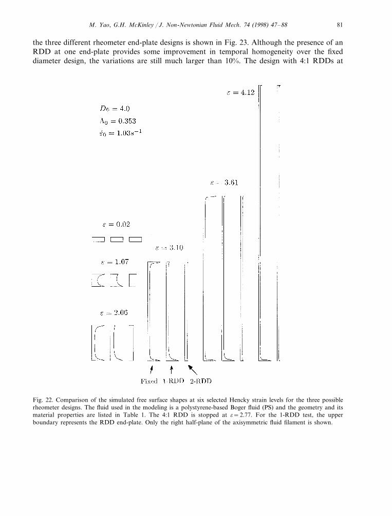
M. Yao, G.H. McKinley / J. Non-Newtonian Fluid Mech. 74 (1998) 47–88 81
the three different rheometer end-plate designs is shown in Fig. 23. Although the presence of anRDD at one end-plate provides some improvement in temporal homogeneity over the fixeddiameter design, the variations are still much larger than 10%. The design with 4:1 RDDs at
Fig. 22. Comparison of the simulated free surface shapes at six selected Hencky strain levels for the three possiblerheometer designs. The fluid used in the modeling is a polystyrene-based Boger fluid (PS) and the geometry and itsmaterial properties are listed in Table 1. The 4:1 RDD is stopped at o=2.77. For the 1-RDD test, the upperboundary represents the RDD end-plate. Only the right half-plane of the axisymmetric fluid filament is shown.
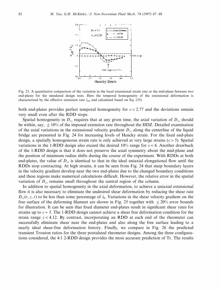
M. Yao, G.H. McKinley / J. Non-Newtonian Fluid Mech. 74 (1997) 47–8882
Fig. 23. A quantitative comparison of the variation in the local extensional strain rate at the mid-plane between twoend-plates for the simulated design tests. Here the temporal homogeneity of the extensional deformation ischaracterized by the effective extension rate o; eff and calculated based on Eq. (35).
both end-plates provides perfect temporal homogeneity for oB2.77 and the deviations remainvery small even after the RDD stops.
Spatial homogeneity in Dzz requires that at any given time, the axial variation of Dzz shouldbe within, say, 910% of the imposed extension rate throughout the HDZ. Detailed examinationof the axial variations in the extensional velocity gradient Dzz along the centerline of the liquidbridge are presented in Fig. 24 for increasing levels of Hencky strain. For the fixed end-platedesign, a spatially homogeneous strain rate is only achieved at very large strains (o\5). Spatialvariations in the 1-RDD design also exceed the desired 10% range for oB4. Another drawbackof the 1-RDD design is that it does not preserve the axial symmetry about the mid-plane andthe position of minimum radius shifts during the course of the experiment. With RDDs at bothend-plates, the value of Dzz is identical to that in the ideal uniaxial elongational flow until theRDDs stop contracting. At high strains, it can be seen from Fig. 24 that steep boundary layersin the velocity gradient develop near the two end-plates due to the changed boundary conditionsand these regions make numerical calculations difficult. However, the relative error in the spatialvariation of Dzz remains small throughout the central region of the column.
In addition to spatial homogeneity in the axial deformation, to achieve a uniaxial extensionalflow it is also necessary to eliminate the undesired shear deformation by reducing the shear rateDrz(r, z, t) to be less than some percentage of o; 0. Variations in the shear velocity gradient on thefree surface of the deforming filament are shown in Fig. 25 together with 920% error boundsfor illustration. It can be seen that fixed diameter end-plates result in significant shear rates forstrains up to o�3. The 1-RDD design cannot achieve a shear free deformation condition for thestrain range oB4.12. By contrast, incorporating an RDD at each end of the rheometer cansuccessfully eliminate shear near the end-plates and also along the free surface leading to anearly ideal shear-free deformation history. Finally, we compare in Fig. 26 the predictedtransient Trouton ratios for the three postulated rheometer designs. Among the three configura-tions considered, the 4:1 2-RDD design provides the most accurate prediction of Tr. The results
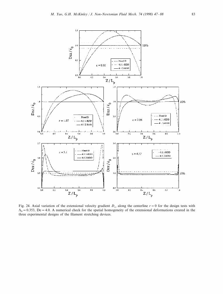
M. Yao, G.H. McKinley / J. Non-Newtonian Fluid Mech. 74 (1998) 47–88 83
Fig. 24. Axial variation of the extensional velocity gradient Dzz along the centerline r=0 for the design tests withL0=0.353, De=4.0. A numerical check for the spatial homogeneity of the extensional deformations created in thethree experimental designs of the filament stretching devices.
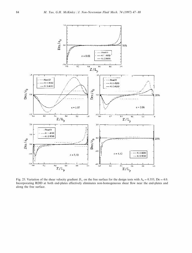
M. Yao, G.H. McKinley / J. Non-Newtonian Fluid Mech. 74 (1997) 47–8884
Fig. 25. Variation of the shear velocity gradient Drz on the free surface for the design tests with L0=0.353, De=4.0.Incorporating RDD at both end-plates effectively eliminates non-homogeneous shear flow near the end-plates andalong the free surface.
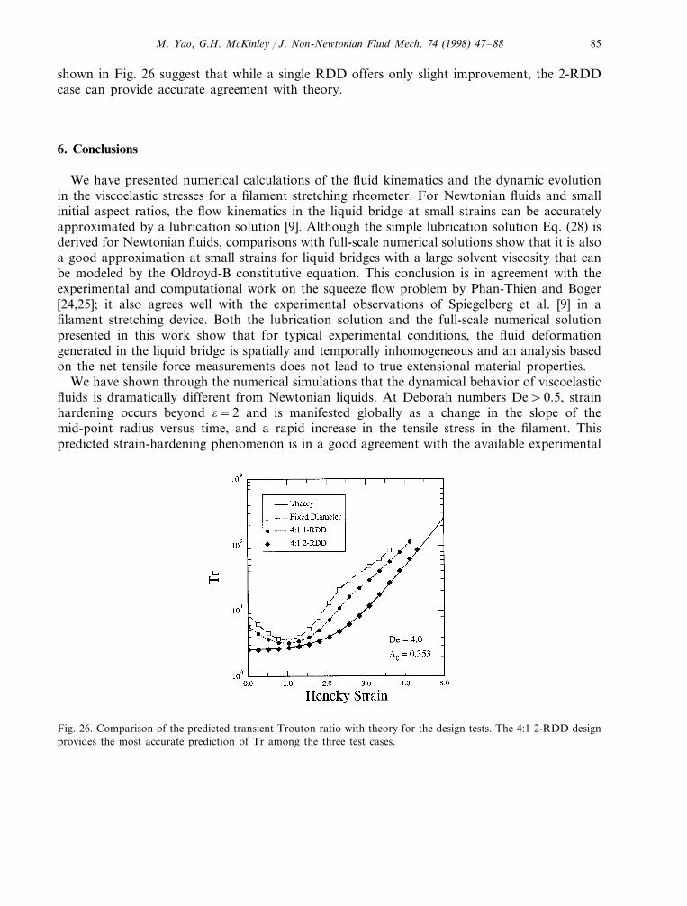
M. Yao, G.H. McKinley / J. Non-Newtonian Fluid Mech. 74 (1998) 47–88 85
shown in Fig. 26 suggest that while a single RDD offers only slight improvement, the 2-RDDcase can provide accurate agreement with theory.
6. Conclusions
We have presented numerical calculations of the fluid kinematics and the dynamic evolutionin the viscoelastic stresses for a filament stretching rheometer. For Newtonian fluids and smallinitial aspect ratios, the flow kinematics in the liquid bridge at small strains can be accuratelyapproximated by a lubrication solution [9]. Although the simple lubrication solution Eq. (28) isderived for Newtonian fluids, comparisons with full-scale numerical solutions show that it is alsoa good approximation at small strains for liquid bridges with a large solvent viscosity that canbe modeled by the Oldroyd-B constitutive equation. This conclusion is in agreement with theexperimental and computational work on the squeeze flow problem by Phan-Thien and Boger[24,25]; it also agrees well with the experimental observations of Spiegelberg et al. [9] in afilament stretching device. Both the lubrication solution and the full-scale numerical solutionpresented in this work show that for typical experimental conditions, the fluid deformationgenerated in the liquid bridge is spatially and temporally inhomogeneous and an analysis basedon the net tensile force measurements does not lead to true extensional material properties.
We have shown through the numerical simulations that the dynamical behavior of viscoelasticfluids is dramatically different from Newtonian liquids. At Deborah numbers De\0.5, strainhardening occurs beyond o=2 and is manifested globally as a change in the slope of themid-point radius versus time, and a rapid increase in the tensile stress in the filament. Thispredicted strain-hardening phenomenon is in a good agreement with the available experimental
Fig. 26. Comparison of the predicted transient Trouton ratio with theory for the design tests. The 4:1 2-RDD designprovides the most accurate prediction of Tr among the three test cases.
M. Yao, G.H. McKinley / J. Non-Newtonian Fluid Mech. 74 (1997) 47–8886
measurements [2,3,7,9] and, in contrast to the evolution of a Newtonian filament, results in theformation of an increasingly uniform cylindrical viscoelastic filament. The predicted break-upmechanism in viscoelastic liquid bridge at high De is also quite different from the Newtoniancase. For Newtonian fluids, there is no strain-hardening and ‘necking’ always decreases thefilament radius fastest at the fluid mid-plane between the two end-plates. Consequently,Newtonian liquid bridges in filament stretching devices will break in the middle. For viscoelasticfluids, the strain hardening at large Hencky strains inhibits the filament from breaking in themiddle. Instead, the rapid amplification of liquid drainage from the end-plate regions willultimately initiate the onset of an elastic instability in the vicinity of the end-plates. Ournumerical calculations of the evolution of the free surface agree well with the experimentalobservations reported in [10] and also with those simulated by Sizaire and Legat using theFENE-CR model [29]. Indeed for the range of strains (o54) covered in [29] and the presentwork, the filament shapes predicted by the FENE-CR and Oldroyd-B models are practicallyindistinguishable. The progressive drainage of the quasi-static fluid reservoirs present at eachrigid end-plate provides a rationalization for the elastic instability and decohesion phenomenaobserved experimentally at large Hencky strains.
As a result of the spatially inhomogeneous deformation at short times, the development of astress localization or ‘boundary layer’ in the polymer stress near the free surface is observed. Inexperiments, such radial stress distributions within the liquid filament are almost impossible tomeasure, and force measurements are interpreted as resulting from a radially uniform fluidstress. The numerical results predict an important difference in the stress behavior between theviscoelastic and the Newtonian liquids. For Newtonian filaments, the local stress concentrationin the vicinity of the mid-point of the free surface is present only at small strains and eventuallydecays at larger strain levels as the extension rate Dzz becomes radially uniform across themid-plane. For the Oldroyd-B fluid with a small initial aspect ratio, the local stress inhomogene-ity evolves with the strain throughout the deformation history and leads to the formation of athin stress boundary layer at larger strains even when a homogeneous extensional strain rate isreached. This stress boundary layer development is a direct consequence of the elastic propertiesof the material, as the viscoelastic liquid ‘remembers’ the non-homogeneous deformation andpre-shearing history it experienced at small strains. Design calculations for different aspect ratiossuggest that the development of the stress boundary layer depends on the initial aspect ratio andcan be eliminated by using larger initial aspect ratios in the design.
Our numerical observations of the stress concentration and boundary layer development agreequalitatively well with the results of the configuration tensor A �QQ�/Q eq
2 given by Sizaireand Legat [29]. Here �QQ� represents an ensemble average over the configuration space of thedyadic product, QQ, of the dumbbell end-to-end vector Q, and Q eq
2 is the mean squareend-to-end distance between the two beads. The radial variation of the extensional componentof the configuration tensor in Fig. 5 of Ref. [29] shows a non-homogeneous extensionaldeformation at the macromolecular level on the mid-point plane. The macromolecules, repre-sented by elastic dumbbells in the kinetic theory, are more elongated near the curved free surfacethan in the central region of the liquid filament. For small initial aspect ratios, this non-homo-geneous microscopic extensional deformation leads to the macroscopic localization of the liquidextension rate and the development of a stress boundary layer observed in the present work.
M. Yao, G.H. McKinley / J. Non-Newtonian Fluid Mech. 74 (1998) 47–88 87
The most effective approach to improving the homogeneity of the flow kinematics at shorttimes is to simultaneously elongate the sample axially and reduce the diameter of the end-platefixtures at an exponential rate. One inherent physical limit with such reducing diameter deviceis that the radial engineering strain attainable, defined by the RDD ratio in Eq. (37), is usuallyrestricted by the mechanical design of the instrument to be much lower than the total axialstrain of the experiment. Analysis indicates that an RDD rate of 3:1 or greater is necessary topreserve homogeneous extensional deformation up to the onset of pronounced strain hardening.Comparisons based on three postulated designs show that introduction of 4:1 RDDs at bothend-plates is good enough for providing a nearly ideal shear-free deformation history andgreatly enhances accuracy in the measurements than with conventional filament stretchingdevices using fixed diameter end-plates. Of course, in the current experimental realizations ofsuch devices, an alternate approach has been to adjust the end-plate boundary data for L: p(t) toresult in exponential decrease in Rmid(t) at all times. While such an approach leads to a temporalhomogeneity in o; eff(t), the fluid deformation remains spatially inhomogeneous. As a result,selection of the ‘correct’ or optimum profile for L: p(t) must be adjusted ad hoc on a fluid-by-fluidand rate-by-rate basis. Now that we have developed a fundamental and systematic understand-ing of the evolution in the shape and kinematics of viscoelastic fluid columns in a filamentstretching rheometer, it will be possible to investigate this more complex boundary motion indetail, and provide heuristic guidelines for optimizing experimental test protocols.
Acknowledgements
This work was supported by NASA’s Microgravity Science and Application Program. Wewould like to thank Benoit Debbaut and Thierry Marchal at Polyflow, s.a. for their technicalsupport for solving moving boundary problems with Polyflow. Computer system and graphicssupport from David A. Thompson at the Computational Material Lab, NASA Lewis ResearchCenter is acknowledged.
References
[1] M.M. Denn, in: J.L. Lumley, A. Acrivos, L.G. Leal, S. Leibovich (Eds.), Research Trends in Fluid Dynamics,AIP Press, Woodbury, New York, 1996, p. 69.
[2] D.F. James, K. Walters, in: A.A. Collyer (Ed.), Techniques in Rheological Measurement, Chapman and Hall,London, 1993, Ch. 2.
[3] T. Sridhar, V. Tirtaatmadja, D.A. Nguyen, R.K. Gupta, J. Non-Newtonian Fluid Mech. 40 (1991) 271.[4] V. Tirtaatmadja, T. Sridhar, J. Rheol. 37 (1993) 1081.[5] R. Kroger, S. Berg, A. Delgado, H.J. Rath, J. Non-Newtonian Fluid Mech. 45 (1992) 385.[6] S. Berg, R. Kroger, H.J. Rath, J. Non-Newtonian Fluid Mech. 55 (1994) 307.[7] M.J. Solomon, S.J. Muller, J. Rheol. 40 (1996) 837.[8] S. Gaudet, G.H. McKinley, H.A. Stone, Phys. Fluids 8 (1996) 2568.[9] S.H. Spiegelberg, D.C. Ables, G.H. McKinley, J. Non-Newtonian Fluid Mech. 64 (1996) 229.
[10] S.H. Spiegelberg, G.H. McKinley, J. Non-Newtonian Fluid Mech. 67 (1996) 49.[11] R.B. Bird, R.C. Armstrong, O. Hassager, Dynamics of Polymeric Liquids, Vol. 1, Fluid Mechanics, 2nd ed.,
Wiley, New York, 1987.
M. Yao, G.H. McKinley / J. Non-Newtonian Fluid Mech. 74 (1997) 47–8888
[12] V. Tirtaatmadja, T. Sridhar, J. Rheol. 39 (1995) 1133.[13] D.F. James, T. Sridhar, J. Rheol. 39 (1995) 713.[14] P.R. Schunk, J.M. de Santos, L.E. Scriven, J. Rheol. 34 (1990) 387.[15] J. Sun, N. Phan-Thien, R.I. Tanner, J. Non-Newtonian Fluid Mech. 58 (1995) 219.[16] R.W.G. Shipman, M.M. Denn, R. Keunings, J. Non-Newtonian Fluid Mech. 40 (1991) 281.[17] J.G. Oldroyd, Proc. R. Soc. A200 (1950) 523.[18] L.A. Slobozhanin, J.M. Perales, Phys. Fluids A5 (1993) 1305.[19] M. Yao, G.H. McKinley, (1996) (in preparation).[20] Polyflow User’s Manual, ver. 3.4.0., Polyflow s.a., Place de l’Universite 16, B-1348, Louvain-la-Neuve, Belgium,
1995.[21] J.F. Thompson, Z.U.A. Warsi, C. Wayne Mastin, Numerical Grid Generation—Foundations and Applications,
Elsevier, Amsterdam, 1985.[22] R.D. Gillette, D.C. Dyson, Chem. Eng. J. 2 (1971) 44.[23] J. Stefan, Sitzungber, K. Akad. Wiss. Math. Natur. Wien 69 (1874) 713.[24] N. Phan-Thien, R.I. Tanner, J. Non-Newtonian Fluid Mech. 14 (1984) 327.[25] N. Phan-Thien, J. Dudek, D.V. Boger, V. Tirtaatmadja, J. Non-Newtonian Fluid Mech. 18 (1985) 227.[26] H.C. Lee, IBM J. Res. Dev. 18 (1974) 364.[27] J. Meseguer, J. Fluid Mech. 130 (1983) 123.[28] S.L. Goren, M. Gottlieb, J. Fluid Mech. 120 (1982) 245.[29] R. Sizaire, V. Legat, J. Non-Newtonian Fluid Mech. 71 (1997) 89–108.