numerical simulation and theoretical analysis of the 3d viscous flow

TASK QUARTERLY 5 No 4 (2001), 433–458

NUMERICAL SIMULATION AND THEORETICALANALYSIS OF THE 3D VISCOUS FLOW

IN CENTRIFUGAL IMPELLERSSHUN KANG AND CHARLES HIRSCH

Vrije Universiteit Brussels,Department of Fluid Mechanics,

Pleinlaan 2, 1050 Brussels, [email protected]

(Received 20 July 2001)

Abstract: This paper investigates the three-dimensional viscous flow in centrifugal impellers through the-oretical analysis and numerical simulations, which is a summary of the authors’ recent work. A quantitativeevaluation of the different contributions to the streamwise vorticity is performed, namely, the passagevortices along the endwalls due to the flow turning; a passage vortex generated by the Coriolis forces pro-portional to the local loading and mainly active in the radial parts of the impeller; blade surface vortices dueto the meridional curvature. In the numerical simulation the NASA Large Scale Centrifugal Compressor(LSCC) impeller with vaneless diffuser is computed at three flow rates. An advanced Navier-Stokes solver,EURANUS/TURBO is applied with an algebraic turbulence model of Badwin-Lomax and a linear k-"model for closure, for different meshes. An in-depth validation has been performed based on the measureddata. An excellent agreement is obtained for most of the data over a wide region of the flow passage.Structures of the 3D flow in the blade passage and the tip region, and their variations with flow rate as well,are analysed based on the numerical results.

Keywords: centrifugal compressor, secondary flow, CFD, tip leakage flows, viscous flow

NomenclatureCp – specific heat at constant pressurep – static pressure, N/m2

pŁ – rotary stagnation pressure, N/m2

Pr – reduced static pressure, N/m2

Pre f – reference pressure, N/m2

Pao – absolute total pressure, N/m2

PS – pressure sideRo – Rossby numberSS – suction sideTao – static temperature, KTu – turbulence intensityU – rotor blade speed, m/sVm – throughflow velocity, m/sV� – tangential absolute velocity, m/s

tq0405c7/433 26I2002 BOP s.c., http://www.bop.com.pl

434 S. Kang and Ch. Hirsch

Vz – axial absolute velocity, m/sW – relative velocity, m/sþ – relative flow angleŽ – boundary layer thickness, m¼l – moleculor viscosity, m2/s¼t – turbulent viscosity, m2/s² – density, kg/m3

¦ – meridional flow angle! – rotation speed, 1/s!s – streamwise vorticity, 1/s

1. IntroductionIn recent years, the 3D flow structure of axial turbines and compressors has been

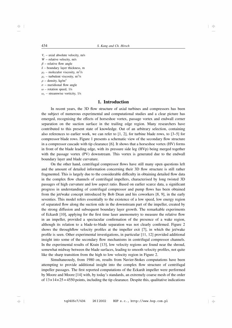
the subject of numerous experimental and computational studies and a clear picture hasemerged, recognising the effects of horseshoe vortex, passage vortex and endwall cornerseparation on the suction surface in the trailing edge region. Many researchers havecontributed to this present state of knowledge. Out of an arbitrary selection, containingalso references to earlier work, we can refer to [1, 2], for turbine blade rows, to [3–5] forcompressor blade rows. Figure 1 presents a schematic view of the secondary flow structurein a compressor cascade with tip clearance [6]. It shows that a horseshoe vortex (HV) formsin front of the blade leading edge, with its pressure side leg (HVp) being merged togetherwith the passage vortex (PV) downstream. This vortex is generated due to the endwallboundary layer and blade curvature.

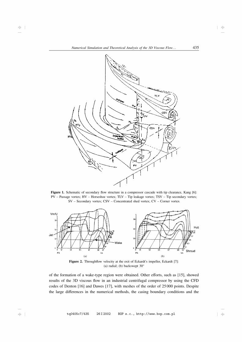
On the other hand, centrifugal compressor flows have still many open questions leftand the amount of detailed information concerning their 3D flow structure is still ratherfragmented. This is largely due to the considerable difficulty in obtaining detailed flow datain the complex flow channels of centrifugal impellers, characterised by long twisted 3Dpassages of high curvature and low aspect ratio. Based on earlier scarce data, a significantprogress in understanding of centrifugal compressor and pump flows has been obtainedfrom the jet/wake concept introduced by Bob Dean and his coworkers [8, 9], in the earlyseventies. This model refers essentially to the existence of a low speed, low energy regionof separated flow along the suction side in the downstream part of the impeller, created bythe strong diffusion and subsequent boundary layer growth. The remarkable experimentsof Eckardt [10], applying for the first time laser anemometry to measure the relative flowin an impeller, provided a spectacular confirmation of the presence of a wake region,although its relation to a blade-to-blade separation was not clearly confirmed. Figure 2shows the throughflow velocity profiles at the impeller exit [7], in which the jet/wakeprofile is seen. Other experimental investigations, in particular [11, 12] provided additionalinsight into some of the secondary flow mechanisms in centrifugal compressor channels.In the experimental results of Krain [13], low velocity regions are found near the shroud,somewhat midway between the blade surfaces, leading to smooth velocity profiles, not quitelike the sharp transition from the high to low velocity region in Figure 2.

Simultaneously, from 1980 on, results from Navier-Stokes computations have beenattempting to provide additional insight into the complex flow structure of centrifugalimpeller passages. The first reported computations of the Eckardt impeller were performedby Moore and Moore [14] with, by today’s standards, an extremely coarse mesh of the orderof 13×14×25 = 4550 points, including the tip clearance. Despite this, qualitative indications


Numerical Simulation and Theoretical Analysis of the 3D Viscous Flow: : : 435

Figure 1. Schematic of secondary flow structure in a compressor cascade with tip clearance, Kang [6]:PV – Passage vortex; HV – Horseshoe vortex; TLV – Tip leakage vortex; TSV – Tip secondary vortex;

SV – Secondary vortex; CSV – Concentrated shed vortex; CV – Corner vortex

(a) (b)

Figure 2. Throughflow velocity at the exit of Eckardt’s impeller, Eckardt [7]:(a) radial; (b) backswept 30°

of the formation of a wake-type region were obtained. Other efforts, such as [15], showedresults of the 3D viscous flow in an industrial centrifugal compressor by using the CFDcodes of Denton [16] and Dawes [17], with meshes of the order of 25000 points. Despitethe large differences in the numerical methods, the casing boundary conditions and the



turbulence models, both codes predicted similar flow fields. Dawes [18] simulated the 3Dunsteady viscous flow in a centrifugal compressor with a vaned diffuser and found that theimpeller flow is essentially steady with a limited influence from the diffuser, vaned or not.These and other computations, such as [19], showed that the gross features of the impellerflows can be captured by the Navier-Stokes computations, even on relatively coarse meshesand simple turbulence models.

However, if CFD is to be applied as a quantitative tool, to compensate for the nearimpossibility of obtaining detailed experimental data of boundary layer and secondaryflows in the complex flow channels of centrifugal machines, more severe requirementshave to be put on the CFD computations and results. In particular, since the secondaryflow intensity is directly related to the stagnation pressure gradients in the boundary layers,sufficient grid resolution has to be provided in order to capture accurately the intensity ofthe secondary flows.

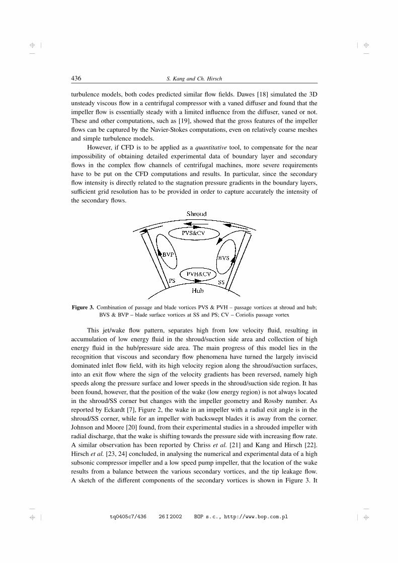
Figure 3. Combination of passage and blade vortices PVS & PVH – passage vortices at shroud and hub;BVS & BVP – blade surface vortices at SS and PS; CV – Coriolis passage vortex

This jet/wake flow pattern, separates high from low velocity fluid, resulting inaccumulation of low energy fluid in the shroud/suction side area and collection of highenergy fluid in the hub/pressure side area. The main progress of this model lies in therecognition that viscous and secondary flow phenomena have turned the largely invisciddominated inlet flow field, with its high velocity region along the shroud/suction surfaces,into an exit flow where the sign of the velocity gradients has been reversed, namely highspeeds along the pressure surface and lower speeds in the shroud/suction side region. It hasbeen found, however, that the position of the wake (low energy region) is not always locatedin the shroud/SS corner but changes with the impeller geometry and Rossby number. Asreported by Eckardt [7], Figure 2, the wake in an impeller with a radial exit angle is in theshroud/SS corner, while for an impeller with backswept blades it is away from the corner.Johnson and Moore [20] found, from their experimental studies in a shrouded impeller withradial discharge, that the wake is shifting towards the pressure side with increasing flow rate.A similar observation has been reported by Chriss et al. [21] and Kang and Hirsch [22].Hirsch et al. [23, 24] concluded, in analysing the numerical and experimental data of a highsubsonic compressor impeller and a low speed pump impeller, that the location of the wakeresults from a balance between the various secondary vortices, and the tip leakage flow.A sketch of the different components of the secondary vortices is shown in Figure 3. It



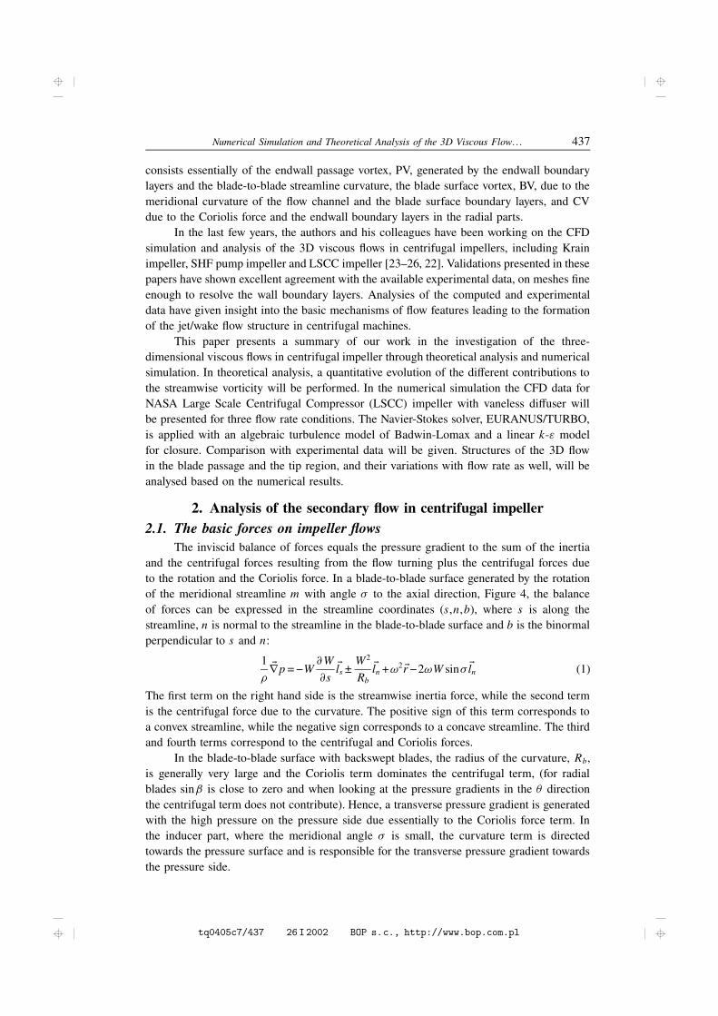
consists essentially of the endwall passage vortex, PV, generated by the endwall boundarylayers and the blade-to-blade streamline curvature, the blade surface vortex, BV, due to themeridional curvature of the flow channel and the blade surface boundary layers, and CVdue to the Coriolis force and the endwall boundary layers in the radial parts.

In the last few years, the authors and his colleagues have been working on the CFDsimulation and analysis of the 3D viscous flows in centrifugal impellers, including Krainimpeller, SHF pump impeller and LSCC impeller [23–26, 22]. Validations presented in thesepapers have shown excellent agreement with the available experimental data, on meshes fineenough to resolve the wall boundary layers. Analysies of the computed and experimentaldata have given insight into the basic mechanisms of flow features leading to the formationof the jet/wake flow structure in centrifugal machines.

This paper presents a summary of our work in the investigation of the three-dimensional viscous flows in centrifugal impeller through theoretical analysis and numericalsimulation. In theoretical analysis, a quantitative evolution of the different contributions tothe streamwise vorticity will be performed. In the numerical simulation the CFD data forNASA Large Scale Centrifugal Compressor (LSCC) impeller with vaneless diffuser willbe presented for three flow rate conditions. The Navier-Stokes solver, EURANUS/TURBO,is applied with an algebraic turbulence model of Badwin-Lomax and a linear k-" modelfor closure. Comparison with experimental data will be given. Structures of the 3D flowin the blade passage and the tip region, and their variations with flow rate as well, will beanalysed based on the numerical results.

2. Analysis of the secondary flow in centrifugal impeller2.1. The basic forces on impeller flows

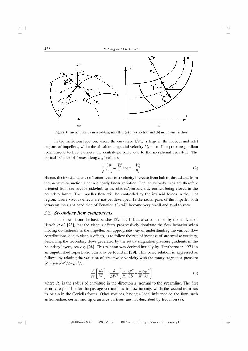
The inviscid balance of forces equals the pressure gradient to the sum of the inertiaand the centrifugal forces resulting from the flow turning plus the centrifugal forces dueto the rotation and the Coriolis force. In a blade-to-blade surface generated by the rotationof the meridional streamline m with angle ¦ to the axial direction, Figure 4, the balanceof forces can be expressed in the streamline coordinates (s,n,b), where s is along thestreamline, n is normal to the streamline in the blade-to-blade surface and b is the binormalperpendicular to s and n:

1²Erp = −W

@W@sEls ±

W2

Rb

Eln +!2Er −2!W sin¦Eln (1)

The first term on the right hand side is the streamwise inertia force, while the second termis the centrifugal force due to the curvature. The positive sign of this term corresponds toa convex streamline, while the negative sign corresponds to a concave streamline. The thirdand fourth terms correspond to the centrifugal and Coriolis forces.

In the blade-to-blade surface with backswept blades, the radius of the curvature, Rb,is generally very large and the Coriolis term dominates the centrifugal term, (for radialblades sinþ is close to zero and when looking at the pressure gradients in the � directionthe centrifugal term does not contribute). Hence, a transverse pressure gradient is generatedwith the high pressure on the pressure side due essentially to the Coriolis force term. Inthe inducer part, where the meridional angle ¦ is small, the curvature term is directedtowards the pressure surface and is responsible for the transverse pressure gradient towardsthe pressure side.



(a) (b)

Figure 4. Inviscid forces in a rotating impeller: (a) cross section and (b) meridional section

In the meridional section, where the curvature 1/Rm is large in the inducer and inletregions of impellers, while the absolute tangential velocity V� is small, a pressure gradientfrom shroud to hub balances the centrifugal force due to the meridional curvature. Thenormal balance of forces along nm leads to:

1²

@p@nm

=V 2�

rcos¦ −

V 2m

Rm(2)

Hence, the invicid balance of forces leads to a velocity increase from hub to shroud and fromthe pressure to suction side in a nearly linear variation. The iso-velocity lines are thereforeoriented from the suction side/hub to the shroud/pressure side corner, being closed in theboundary layers. The impeller flow will be controlled by the inviscid forces in the inletregion, where viscous effects are not yet developed. In the radial parts of the impeller bothterms on the right hand side of Equation (2) will become very small and tend to zero.

2.2. Secondary flow componentsIt is known from the basic studies [27, 11, 15], as also confirmed by the analysis of

Hirsch et al. [23], that the viscous effects progressively dominate the flow behavior whenmoving downstream in the impeller. An appropriate way of understanding the various flowcontributions, due to viscous effects, is to follow the rate of increase of streamwise vorticity,describing the secondary flows generated by the rotary stagnation pressure gradients in theboundary layers, see e.g. [28]. This relation was derived initially by Hawthorne in 1974 inan unpublished report, and can also be found in [29]. This basic relation is expressed asfollows, by relating the variation of streamwise vorticity with the rotary stagnation pressurepŁ = p+²W2/2−²u2/2:

@

@s

��s

W

½=

2²W2

�1Rn

@pŁ

@b+!

W@pŁ

@z

½(3)

where Rn is the radius of curvature in the direction n, normal to the streamline. The firstterm is responsible for the passage vortices due to flow turning, while the second term hasits origin in the Coriolis forces. Other vortices, having a local influence on the flow, suchas horseshoe, corner and tip clearance vortices, are not described by Equation (3).



Due to the geometry of centrifugal impellers, the blade-to-blade curvature willgenerate secondary flow due to the hub and shroud boundary layers (the passage vortices,PV), Figure 3, while the meridional curvature will induce secondary flows due to theboundary layers developing along the blade surfaces (the blade surface vortices, BV). Thesecond term, originating from the Coriolis forces, will be effective if a boundary layergradient exists in the axial direction. This will be the case for the endwall boundarylayer in the radial parts of the impeller, where they will be contributing to the passagevortices (Coriolis passage vortices, CV). If the inducer blade geometry is at an angle to theaxial direction, the blade boundary layers will contribute an axial component of the bladestagnation pressure loss gradients. This contribution is expected to be small and will notbe considered here.

The passage vortices drive low energy fluid from the pressure towards the suctionsurface along hub and shroud walls, while the blade surface vortices generate flowcomponents along the blade surfaces from hub to shroud. The resulting motion leads toan accumulation of low velocity, high loss fluid towards the suction surface region, calledthe wake region. The resulting position of this wake region will depend on the balancebetween these different vortices.

The intensity of individual vortices shown in Figure 3 can then be estimated fromEquation (3) following [24], considering that the reduced static pressure [p−²(r!)2/2] doesnot vary significantly in the boundary layers.

2.2.1. Passage vortex from blade-to-blade curvature

This curvature will generate the endwall vortex PVs and PVh, due to the endwallboundary layers. The intensity of these vortices can be obtained from Equation (3) as:

d��s

W

½

PV /h,s

=2W

1Rb

�@W@b

½

h,s

ds =2W

�@W@b

½

h,s

dþ (4)

where dþ = ds/Rb. Hence, the contribution will vanish locally for radial ending blades,in absence of backsweep. This equation can also be approximately expressed in anotherway as:

d��s

W

½

PV /h,s

=2W

1Rb

�@W@b

½

h,s

ds³ 2W

1Rb

WŽh,s

ds³ 2Rb

dsŽh,s

(5)

where Žh,s is the thickness of hub and shroud boundary layers and Rb the curvature radiusof streamlines in the blade-to-blade surface.

2.2.2. Blade surface vortices

In a similar way, the intensity of the blade surface vortices BV can be estimated,leading to:

d��s

W

½

BV /ps,ss

=2W

1Rm

�@W@b

½

ps,ss

ds³ 2Rm

dsŽPS,SS

(6)

where ŽPS,SS is the thickness of hub and shroud boundary layer and Rm the curvature radiusof streamlines in the meridional surface. It can be seen that increasing the channel curvature1/Rm increases the blade surface vortices. This contribution will not grow in the radial partsof impellers, where 1/Rm tends to zero.



2.2.3. Passage vortices from Coriolis forces

The second term of Equation (3) is significant where the hub and shroud normalshave axial components, that is in the radial portions of the impeller. The Coriolis vortexCV can be estimated from Equation (3) as:

d��s

W

½

CV /h,s

=2²W2

!

W

�@pŁ

@z

½³ !

WdsŽh,s

(7)

Or, as in [24], it can also be expressed as:

d��s

W

½

CV /h,s

=2

Wm

1Wps

pŽh,sds (8)

where p is the pitch. It can be seen that the contribution to the passage vortex variationis proportional to the loading 1Wps and inversely proportional to the meridional velocity,that is to mass flow rate. In other words, the intensity of the vortex CV is proportional tothe rotationaly speed as this loading is produced by the Coriolis effect but not the blade-to-blade curvature. This component of the secondary flow will tend to become dominant inthe radial parts of impellers.

2.2.4. Balance of the vortices

The location, size, and the level of energy loss, of the wake depend on the balance ofall these vortices. This balance can be described by the ratio of the streamwise incrementsof the passage vortex (PV and CV) to the blade surface vortex (BV), leading to:

þþþþþdð�sW

Łh,s

+dð�sW

ŁCV

dð�sW

ŁBV

þþþþþ³ŽPS,SS

Žh,s

�Rm

Rb+!Rm

W

�³ ŽPS,SS

Žh,s

�1þ

1¦+

1Ro

�(9)

where 1þ is the overall turning from the impeller inlet to the exit, 1¦ the flow turningangle in the meridional surface, and Ro= W /!Rm the Rossby number. It can be seen fromEquation (9) that the balance of the blade surface vortices and the passage vortices dependson the ratio of the streamline curvatures in the blade-to-blade and meridional surfaces, theRossby number and the ratio of the boundary layer thicknesses of the endwalls and theblade surfaces. The ratio of the boundary layer thicknesses could be close to one for mostof the practically used machines. Hence the important contributions are from the impellergeometry and the Rossby number. Reducing the overall turning angle, such as applyingbacksweep to the blade profile, the endwall passage vortices will become less important,resulting in the wake position being shifted away from the shroud/SS corner towards thepressure side, as seen from Figure 2.

For a given impeller, its discharge flow profile will depend on its rotational speed andthe flow rate, that is, the Rossby number. The influence of the Rossby number on the wakelocation has been reported by Johnson and Moore [20]. They found, from their experimentalstudies in a shrouded impeller with radial discharge, that the wake is located on the suctionsurface in the ’below design’ flow, near the shroud/SS corner in the ’design flow’ and onthe shroud in the ’above design’ flow. This is due to the progressively dominating effect ofthe BV on the (PV + CV) when mass flow is increased.

In addition, contributions of tip leakage flow to the wake position are not included inEquation (9). In an unshrouded impeller, the tip leakage flow acts in a direction opposite tothe shroud passage vortex and tends to move the endwall fluid from the shroud/SS corner



towards the pressure side. As discussed in [26, 22], Equation (9) deduced for a shroudedimpeller, holds also for an impeller with tip clearance.

3. Brief description of the LSCCThe LSCC (Low Speed Centrifugal Compressor) is an experimental facility designed

to duplicate the essential flow physics of high-speed subsonic centrifugal compressor flowfields in a large size, low-speed machine. A complete description of the facility can befound in [30].

The compressor has a backswept impeller, followed by a vaneless diffuser. Theimpeller has 20 full blades with a backsweep of 55°. The inlet diameter is 0.870m andthe inlet blade height is 0.218m. The exit diameter is 1.524m and exit blade height is0.141m. The tip clearance between the blade tip and the shroud is 2.54mm, and is constantfrom the impeller inlet to exit. The design tip speed is 153m/s, with a rotation speed of1862rpm and a design mass flow of 30kg/s. The experimental measurements include staticpressures on blade surfaces and shroud wall, velocity components with laser anemometerat 18 cross-sections from the upstream to downstream of the impeller.

4. Numerical calculation methodIn all computations, the Navier-Stokes code EURANUS integrated in the Fine/Turbo

interface by NUMECA International, was used. This software, already presented in [31],solves the time-dependent Reynolds averaged Navier-Stokes equations, with either thealgebraic turbulence model of Baldwin-Lomax or a two-equation k-" model for closure.It is based on a structured multiblock, multigrid approach, including non-matching blockboundaries and incorporates various numerical schemes, based on either a central oran upwind discretization.

For the present calculations, the linear k-" model of Yang and Shih [32], modified byKhodak and Hirsch [33], is selected, in which the damped function used in the eddy viscosityis chosen to be a function of Ry = (k1/2y/v). For comparison, computations with the algebraicturbulence model of Baldwin-Lomax were also done. The calculations were performed witha second-order centered scheme, with second and fourth order artificial dissipation terms anda W-cycle multigrid technique. The numerical procedure applied a four-stage Runge-Kuttascheme, coupled to local time stepping and implicit residual smoothing for convergenceacceleration.

4.1. Computational gridA grid with three blocks, obtained with the auto-grid generation software IGG/Auto-

Grid of NUMECA, is used in this study. The first block covers the flow passage, extendedfrom 40% meridional shroud length upstream of the impeller, to 15% impeller tip radiusdownstream in the radial direction. The second block represents the region behind the blunttrailing edge. The third block occupies the space in the tip gap. A blunt blade tip is meshed,even though the real tested blade tips are rounded as reported by Chriss et al. [21]. Themesh consists of 61×73×129, 13×73×33 and 13×13×65 points, in the tangential, radialand streamwise directions, for blocks 1, 2 and 3, respectively. Hence there are 13 lines overthe gap height and 13 lines across the blade profile. This mesh is named as the Basic Mesh.To investigate the mesh dependence, two other meshes, Coarse Mesh and Fine Mesh listedin Table 1, were also computed.



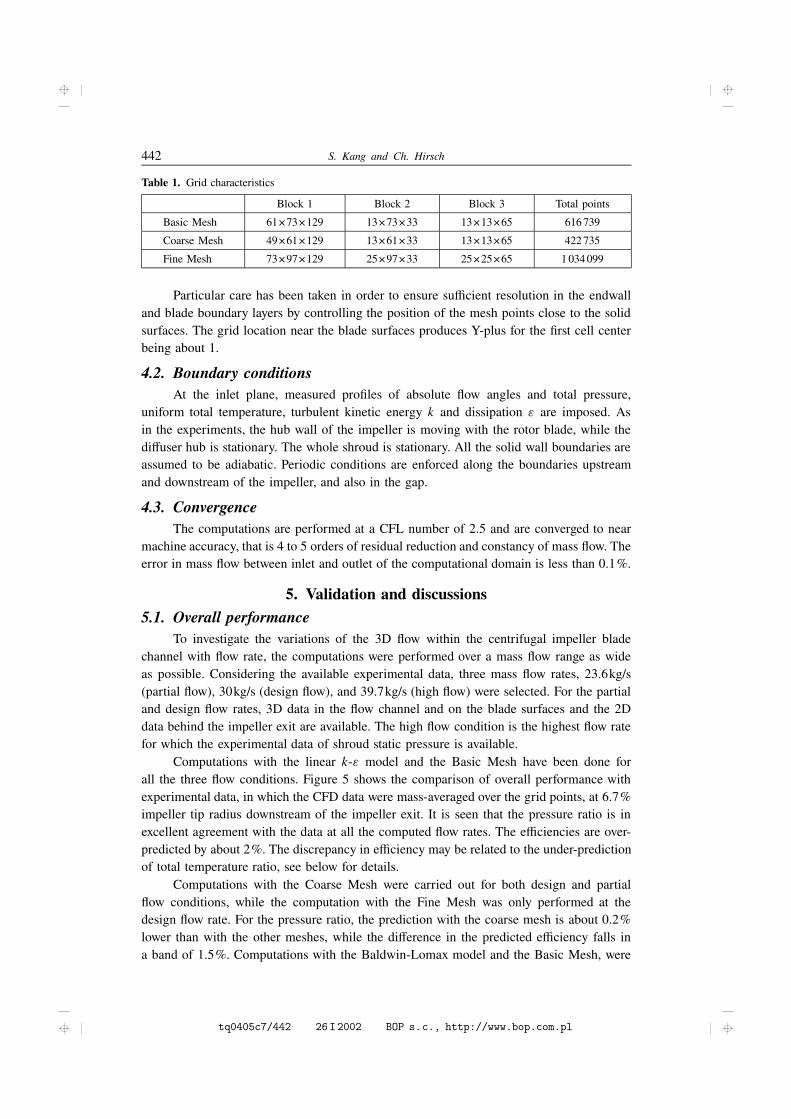
Table 1. Grid characteristics

Block 1 Block 2 Block 3 Total points

Basic Mesh 61×73×129 13×73×33 13×13×65 616739

Coarse Mesh 49×61×129 13×61×33 13×13×65 422735

Fine Mesh 73×97×129 25×97×33 25×25×65 1034099

Particular care has been taken in order to ensure sufficient resolution in the endwalland blade boundary layers by controlling the position of the mesh points close to the solidsurfaces. The grid location near the blade surfaces produces Y-plus for the first cell centerbeing about 1.

4.2. Boundary conditionsAt the inlet plane, measured profiles of absolute flow angles and total pressure,

uniform total temperature, turbulent kinetic energy k and dissipation " are imposed. Asin the experiments, the hub wall of the impeller is moving with the rotor blade, while thediffuser hub is stationary. The whole shroud is stationary. All the solid wall boundaries areassumed to be adiabatic. Periodic conditions are enforced along the boundaries upstreamand downstream of the impeller, and also in the gap.

4.3. ConvergenceThe computations are performed at a CFL number of 2.5 and are converged to near

machine accuracy, that is 4 to 5 orders of residual reduction and constancy of mass flow. Theerror in mass flow between inlet and outlet of the computational domain is less than 0.1%.

5. Validation and discussions5.1. Overall performance

To investigate the variations of the 3D flow within the centrifugal impeller bladechannel with flow rate, the computations were performed over a mass flow range as wideas possible. Considering the available experimental data, three mass flow rates, 23.6kg/s(partial flow), 30kg/s (design flow), and 39.7kg/s (high flow) were selected. For the partialand design flow rates, 3D data in the flow channel and on the blade surfaces and the 2Ddata behind the impeller exit are available. The high flow condition is the highest flow ratefor which the experimental data of shroud static pressure is available.

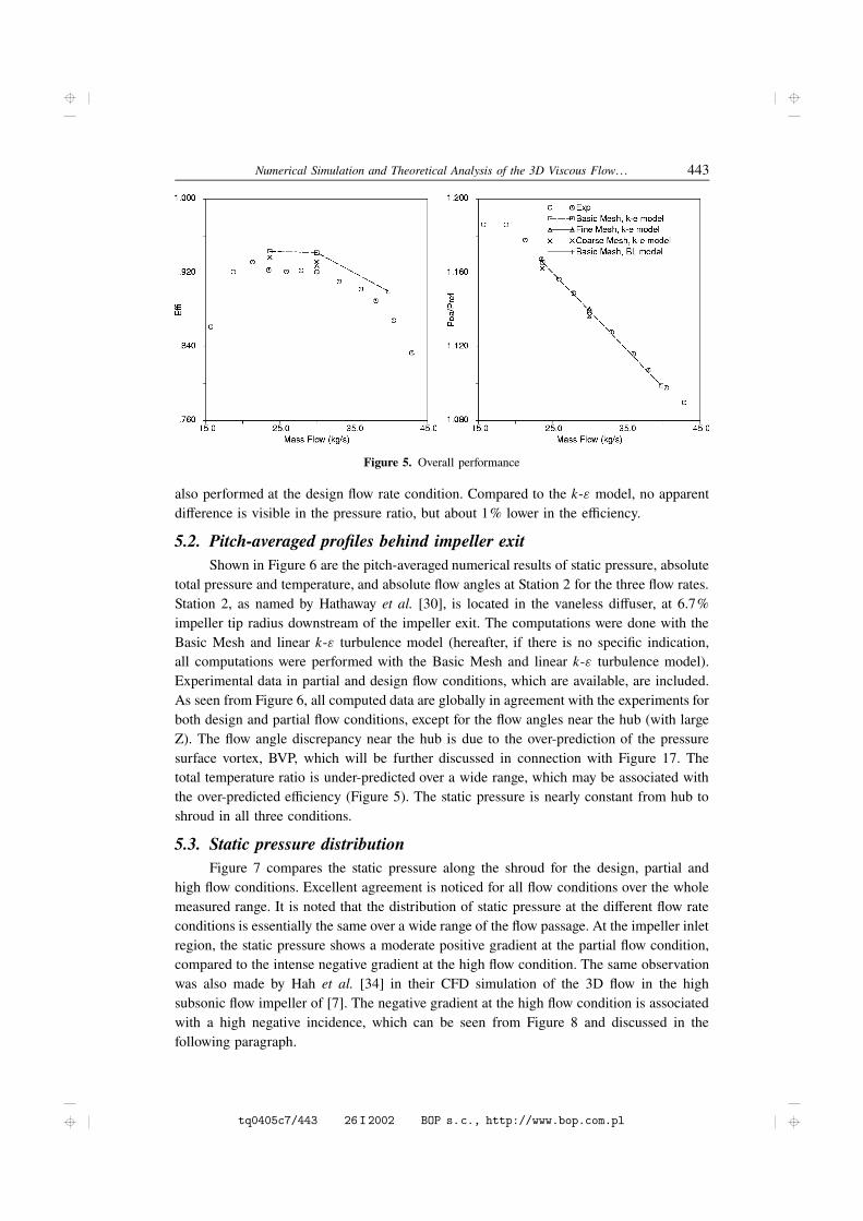
Computations with the linear k-" model and the Basic Mesh have been done forall the three flow conditions. Figure 5 shows the comparison of overall performance withexperimental data, in which the CFD data were mass-averaged over the grid points, at 6.7%impeller tip radius downstream of the impeller exit. It is seen that the pressure ratio is inexcellent agreement with the data at all the computed flow rates. The efficiencies are over-predicted by about 2%. The discrepancy in efficiency may be related to the under-predictionof total temperature ratio, see below for details.

Computations with the Coarse Mesh were carried out for both design and partialflow conditions, while the computation with the Fine Mesh was only performed at thedesign flow rate. For the pressure ratio, the prediction with the coarse mesh is about 0.2%lower than with the other meshes, while the difference in the predicted efficiency falls ina band of 1.5%. Computations with the Baldwin-Lomax model and the Basic Mesh, were



Figure 5. Overall performance

also performed at the design flow rate condition. Compared to the k-" model, no apparentdifference is visible in the pressure ratio, but about 1% lower in the efficiency.

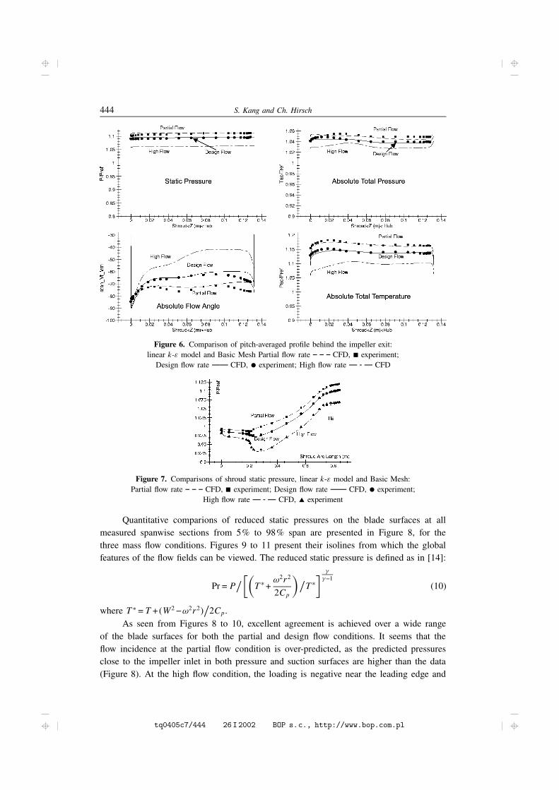
5.2. Pitch-averaged profiles behind impeller exitShown in Figure 6 are the pitch-averaged numerical results of static pressure, absolute

total pressure and temperature, and absolute flow angles at Station 2 for the three flow rates.Station 2, as named by Hathaway et al. [30], is located in the vaneless diffuser, at 6.7%impeller tip radius downstream of the impeller exit. The computations were done with theBasic Mesh and linear k-" turbulence model (hereafter, if there is no specific indication,all computations were performed with the Basic Mesh and linear k-" turbulence model).Experimental data in partial and design flow conditions, which are available, are included.As seen from Figure 6, all computed data are globally in agreement with the experiments forboth design and partial flow conditions, except for the flow angles near the hub (with largeZ). The flow angle discrepancy near the hub is due to the over-prediction of the pressuresurface vortex, BVP, which will be further discussed in connection with Figure 17. Thetotal temperature ratio is under-predicted over a wide range, which may be associated withthe over-predicted efficiency (Figure 5). The static pressure is nearly constant from hub toshroud in all three conditions.

5.3. Static pressure distributionFigure 7 compares the static pressure along the shroud for the design, partial and

high flow conditions. Excellent agreement is noticed for all flow conditions over the wholemeasured range. It is noted that the distribution of static pressure at the different flow rateconditions is essentially the same over a wide range of the flow passage. At the impeller inletregion, the static pressure shows a moderate positive gradient at the partial flow condition,compared to the intense negative gradient at the high flow condition. The same observationwas also made by Hah et al. [34] in their CFD simulation of the 3D flow in the highsubsonic flow impeller of [7]. The negative gradient at the high flow condition is associatedwith a high negative incidence, which can be seen from Figure 8 and discussed in thefollowing paragraph.



Figure 6. Comparison of pitch-averaged profile behind the impeller exit:linear k-" model and Basic Mesh Partial flow rate – – – CFD, S experiment;

Design flow rate —— CFD, C experiment; High flow rate — – — CFD

Figure 7. Comparisons of shroud static pressure, linear k-" model and Basic Mesh:Partial flow rate – – – CFD, S experiment; Design flow rate —— CFD, C experiment;

High flow rate — – — CFD, T experiment

Quantitative comparions of reduced static pressures on the blade surfaces at allmeasured spanwise sections from 5% to 98% span are presented in Figure 8, for thethree mass flow conditions. Figures 9 to 11 present their isolines from which the globalfeatures of the flow fields can be viewed. The reduced static pressure is defined as in [14]:

Pr = PŽ��

T Ł+!2r2

2Cp

�ŽT Ł½

−1(10)

where T Ł = T +(W2 −!2r2)Ž2Cp.

As seen from Figures 8 to 10, excellent agreement is achieved over a wide rangeof the blade surfaces for both the partial and design flow conditions. It seems that theflow incidence at the partial flow condition is over-predicted, as the predicted pressuresclose to the impeller inlet in both pressure and suction surfaces are higher than the data(Figure 8). At the high flow condition, the loading is negative near the leading edge and



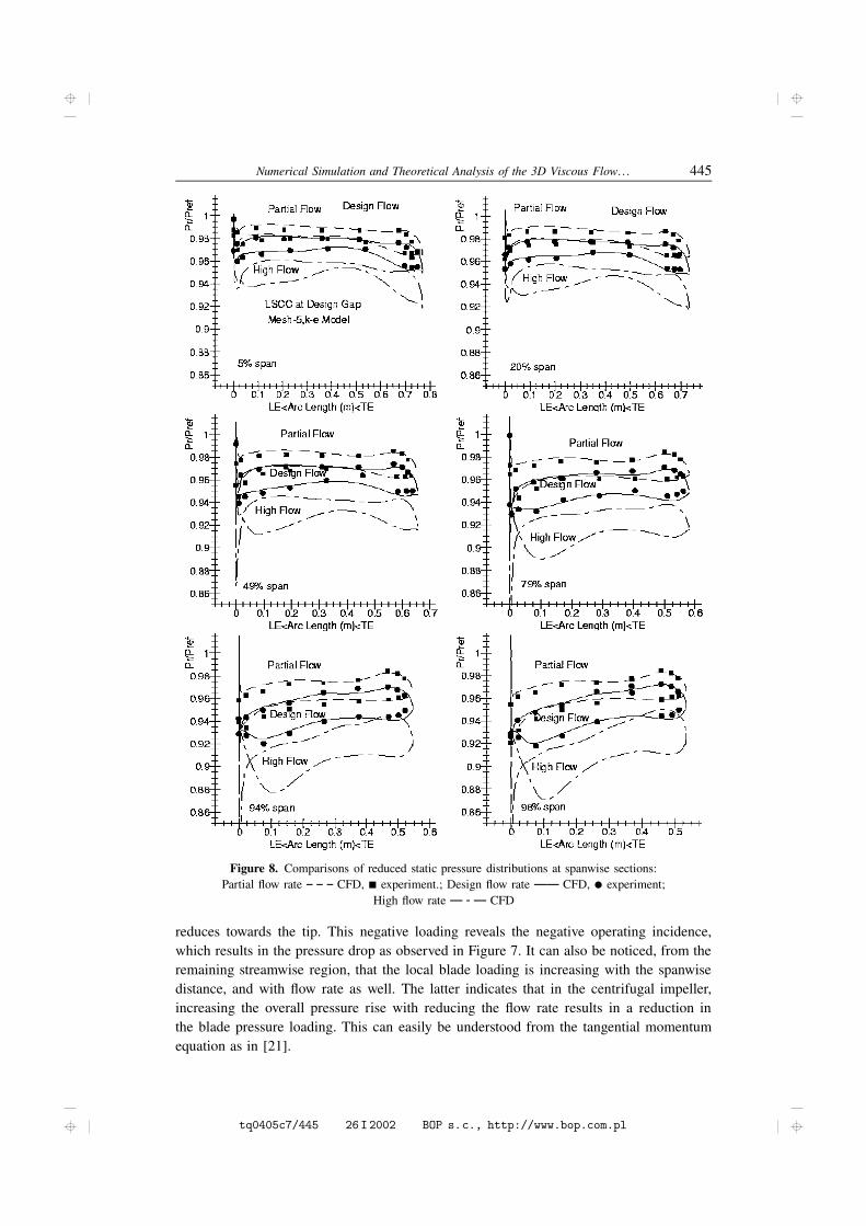
Figure 8. Comparisons of reduced static pressure distributions at spanwise sections:Partial flow rate – – – CFD, S experiment.; Design flow rate —— CFD, C experiment;

High flow rate — – — CFD

reduces towards the tip. This negative loading reveals the negative operating incidence,which results in the pressure drop as observed in Figure 7. It can also be noticed, from theremaining streamwise region, that the local blade loading is increasing with the spanwisedistance, and with flow rate as well. The latter indicates that in the centrifugal impeller,increasing the overall pressure rise with reducing the flow rate results in a reduction inthe blade pressure loading. This can easily be understood from the tangential momentumequation as in [21].



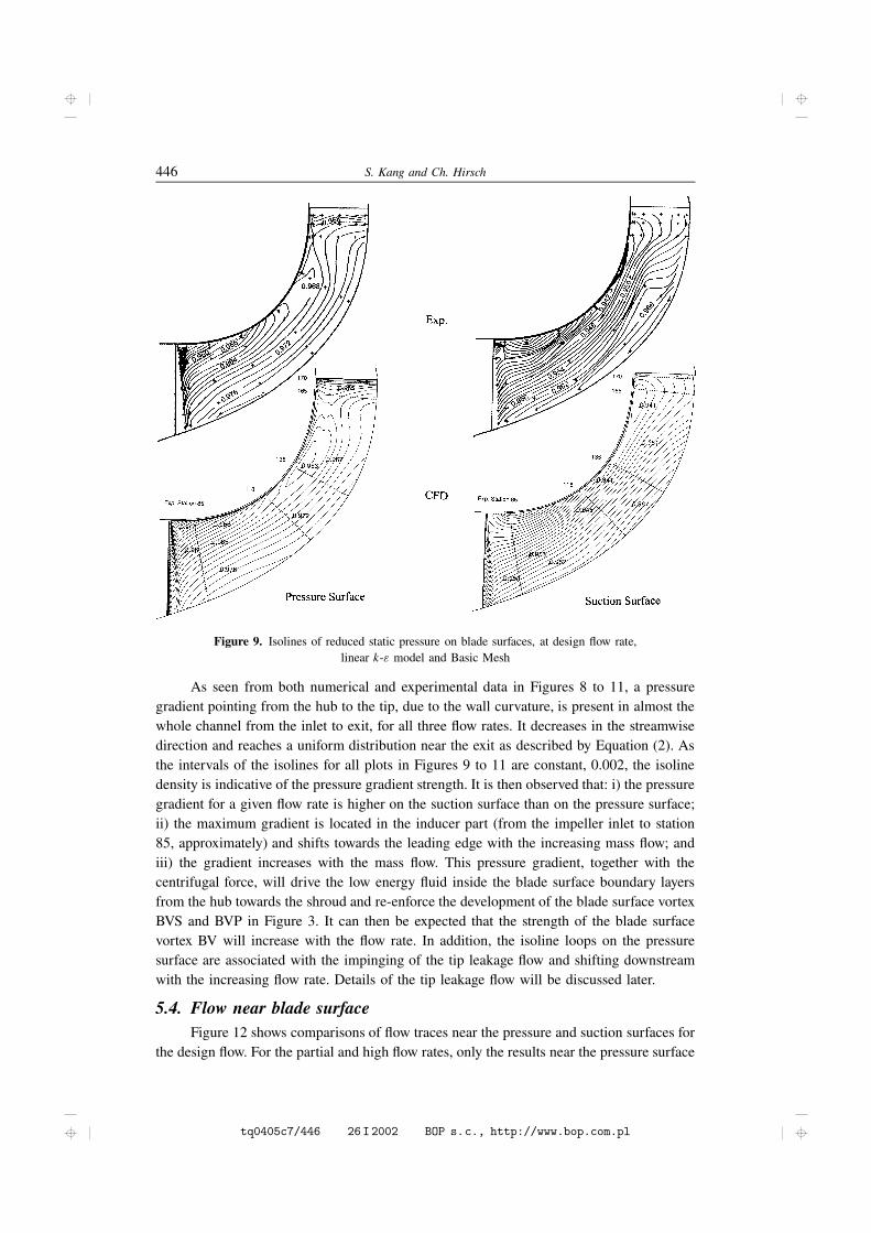
Figure 9. Isolines of reduced static pressure on blade surfaces, at design flow rate,linear k-" model and Basic Mesh

As seen from both numerical and experimental data in Figures 8 to 11, a pressuregradient pointing from the hub to the tip, due to the wall curvature, is present in almost thewhole channel from the inlet to exit, for all three flow rates. It decreases in the streamwisedirection and reaches a uniform distribution near the exit as described by Equation (2). Asthe intervals of the isolines for all plots in Figures 9 to 11 are constant, 0.002, the isolinedensity is indicative of the pressure gradient strength. It is then observed that: i) the pressuregradient for a given flow rate is higher on the suction surface than on the pressure surface;ii) the maximum gradient is located in the inducer part (from the impeller inlet to station85, approximately) and shifts towards the leading edge with the increasing mass flow; andiii) the gradient increases with the mass flow. This pressure gradient, together with thecentrifugal force, will drive the low energy fluid inside the blade surface boundary layersfrom the hub towards the shroud and re-enforce the development of the blade surface vortexBVS and BVP in Figure 3. It can then be expected that the strength of the blade surfacevortex BV will increase with the flow rate. In addition, the isoline loops on the pressuresurface are associated with the impinging of the tip leakage flow and shifting downstreamwith the increasing flow rate. Details of the tip leakage flow will be discussed later.

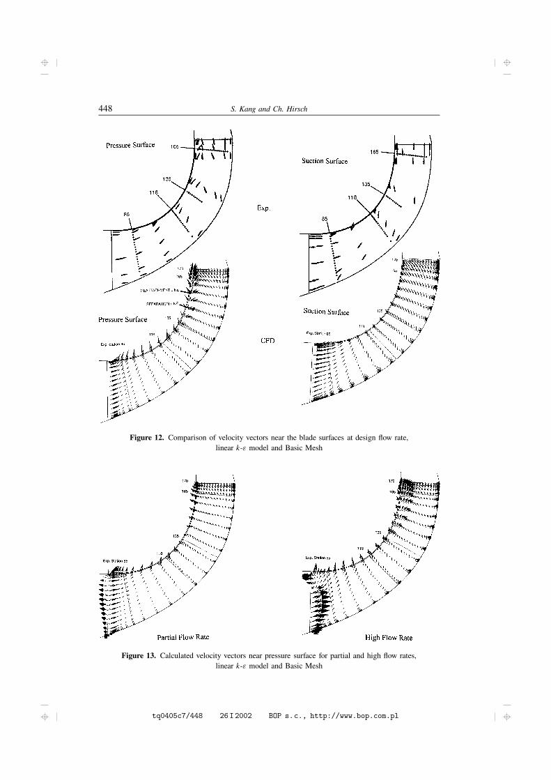
5.4. Flow near blade surfaceFigure 12 shows comparisons of flow traces near the pressure and suction surfaces for

the design flow. For the partial and high flow rates, only the results near the pressure surface



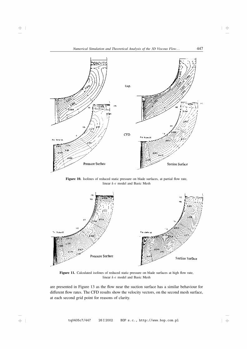
Figure 10. Isolines of reduced static pressure on blade surfaces, at partial flow rate,linear k-" model and Basic Mesh

Figure 11. Calculated isolines of reduced static pressure on blade surfaces at high flow rate,linear k-" model and Basic Mesh

are presented in Figure 13 as the flow near the suction surface has a similar behaviour fordifferent flow rates. The CFD results show the velocity vectors, on the second mesh surface,at each second grid point for reasons of clarity.



Figure 12. Comparison of velocity vectors near the blade surfaces at design flow rate,linear k-" model and Basic Mesh

Figure 13. Calculated velocity vectors near pressure surface for partial and high flow rates,linear k-" model and Basic Mesh



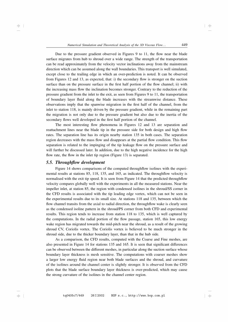
Due to the pressure gradient observed in Figures 9 to 11, the flow near the bladesurface migrates from hub to shroud over a wide range. The strength of the transportationcan be read approximately from the velocity vector inclinations away from the mainstreamdirection which can be assumed along the wall boundaries. This transport is well simulated,except close to the trailing edge in which an over-prediction is noted. It can be observedfrom Figures 12 and 13, as expected, that: i) the secondary flow is stronger on the suctionsurface than on the pressure surface in the first half portion of the flow channel; ii) withthe increasing mass flow the inclination becomes stronger. Contrary to the reduction of thepressure gradient from the inlet to the exit, as seen from Figures 9 to 11, the transportationof boundary layer fluid along the blade increases with the streamwise distance. Theseobservations imply that the spanwise migration in the first half of the channel, from theinlet to station 118, is mainly driven by the pressure gradient, while in the remaining partthe migration is not only due to the pressure gradient but also due to the inertia of thesecondary flows well developed in the first half portion of the channel.

The most interesting flow phenomena in Figures 12 and 13 are separation andreattachment lines near the blade tip in the pressure side for both design and high flowrates. The separation line has its origin nearby station 135 in both cases. The separationregion decreases with the mass flow and disappears at the partial flow condition. This flowseparation is related to the impinging of the tip leakage flow on the pressure surface andwill further be discussed later. In addition, due to the high negative incidence for the highflow rate, the flow in the inlet tip region (Figure 13) is separated.

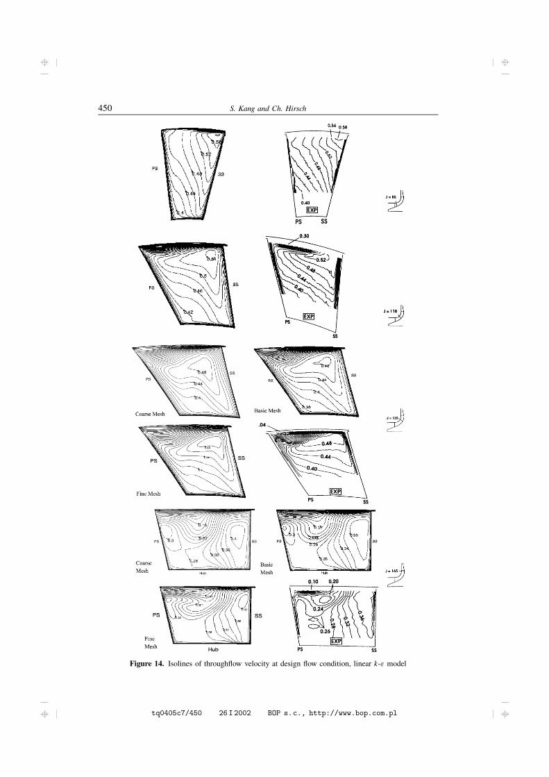
5.5. Throughflow developmentFigure 14 shows comparisons of the computed throughflow isolines with the experi-

mental results at stations 85, 118, 135, and 165, as indicated. The throughflow velocity isnormalised with the exit tip speed. It is seen from Figure 14 that the predicted throughflowvelocity compares globally well with the experiments in all the measured stations. Near theimpeller inlet, at station 85, the region with condensed isolines in the shroud/SS corner inthe CFD results is associated with the tip leading edge vortex, which can not be seen inthe experimental results due to its small size. At stations 118 and 135, between which theflow channel transits from the axial to radial direction, the throughflow wake is clearly seenas the condensed isoline pattern in the shroud/PS corner from both CFD and experimentalresults. This region tends to increase from station 118 to 135, which is well captured bythe computations. In the radial portion of the flow passage, station 165, this low energywake region has migrated towards the mid-pitch near the shroud, as a result of the growingshroud CV, Coriolis vortex. The Coriolis vortex is believed to be much stronger in theshroud side, due to the thicker boundary layer, than that in the hub side.

As a comparison, the CFD results, computed with the Coarse and Fine meshes, arealso presented in Figure 14 for stations 135 and 165. It is seen that significant differencescan be observed between the different meshes, in particular along the suction surface whoseboundary layer thickness is mesh sensitive. The computations with coarser meshes showa larger low energy fluid region near both blade surfaces and the shroud, and curvatureof the isolines around the channel center is slightly stronger. It is observed from the CFDplots that the blade surface boundary layer thickness is over-predicted, which may causethe strong curvature of the isolines in the channel center region.



Figure 14. Isolines of throughflow velocity at design flow condition, linear k-" model



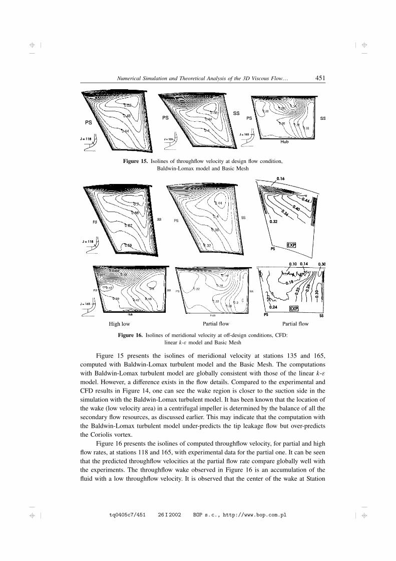
Figure 15. Isolines of throughflow velocity at design flow condition,Baldwin-Lomax model and Basic Mesh

Figure 16. Isolines of meridional velocity at off-design conditions, CFD:linear k-" model and Basic Mesh

Figure 15 presents the isolines of meridional velocity at stations 135 and 165,computed with Baldwin-Lomax turbulent model and the Basic Mesh. The computationswith Baldwin-Lomax turbulent model are globally consistent with those of the linear k-"model. However, a difference exists in the flow details. Compared to the experimental andCFD results in Figure 14, one can see the wake region is closer to the suction side in thesimulation with the Baldwin-Lomax turbulent model. It has been known that the location ofthe wake (low velocity area) in a centrifugal impeller is determined by the balance of all thesecondary flow resources, as discussed earlier. This may indicate that the computation withthe Baldwin-Lomax turbulent model under-predicts the tip leakage flow but over-predictsthe Coriolis vortex.

Figure 16 presents the isolines of computed throughflow velocity, for partial and highflow rates, at stations 118 and 165, with experimental data for the partial one. It can be seenthat the predicted throughflow velocities at the partial flow rate compare globally well withthe experiments. The throughflow wake observed in Figure 16 is an accumulation of thefluid with a low throughflow velocity. It is observed that the center of the wake at Station



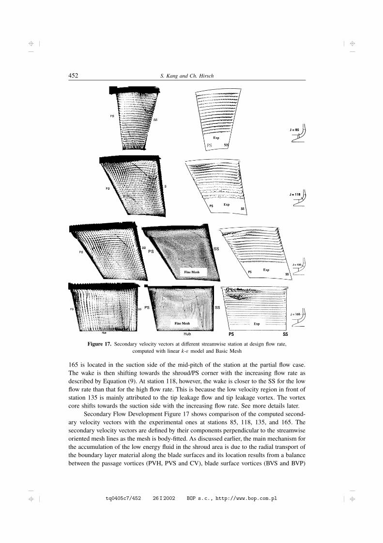
Figure 17. Secondary velocity vectors at different streamwise station at design flow rate,computed with linear k-" model and Basic Mesh

165 is located in the suction side of the mid-pitch of the station at the partial flow case.The wake is then shifting towards the shroud/PS corner with the increasing flow rate asdescribed by Equation (9). At station 118, however, the wake is closer to the SS for the lowflow rate than that for the high flow rate. This is because the low velocity region in front ofstation 135 is mainly attributed to the tip leakage flow and tip leakage vortex. The vortexcore shifts towards the suction side with the increasing flow rate. See more details later.

Secondary Flow Development Figure 17 shows comparison of the computed second-ary velocity vectors with the experimental ones at stations 85, 118, 135, and 165. Thesecondary velocity vectors are defined by their components perpendicular to the streamwiseoriented mesh lines as the mesh is body-fitted. As discussed earlier, the main mechanism forthe accumulation of the low energy fluid in the shroud area is due to the radial transport ofthe boundary layer material along the blade surfaces and its location results from a balancebetween the passage vortices (PVH, PVS and CV), blade surface vortices (BVS and BVP)



and tip leakage flow. All these vortices can also be seen from both CFD and experimentalplots in Figure 17. However, differences between the CFD results and the experimental onesare obvious. It is seen in stations 118 and 135 that the sizes of the computed BVP and BVSare larger than those of the experiments, which is related to the over-predicted boundarylayer thickness as seen from Figure 14. The second difference exists in the shroud/PS cornerin station 135. In the experiment, a well-behaved vortex is observed in the shroud/PS corner.It is the tip leakage vortex and has its origin at the tip leading edge. Downstream of station135, this vortex tends to move away from the corner towards the channel center, drivenby the pressure surface vortex BVP. It seems that the diffusion of the predicted vortex ismuch faster than in the experiments, which may be connected to the fact that the computa-tional results are still mesh dependent. The third difference lies in the shroud/PS corner instation 165. In the experiment, the most dominant flow feature is the strong flow reversalof the spanwise flow direction in the corner. This reversal of flow direction, coupled toan observed high level of velocity fluctuations was explained as local flow unsteadiness byChriss et al. [21]. From the CFD results, this observed unsteadiness might be connected tothe high shear region where strong interactions exist between the two oppositely movingflows, the tip leakage flow and the flow induced by BVP. Another difference in station 165is the vortex motion near the channel center in the CFD plot but not in the experiment. Thisvortex is the pressure surface vortex, BVP. Due to its strong motion, a short distance abovethe hub wall, the flow transports from the suction to the pressure side, which explains theover-predicted flow angle in Figure 6.

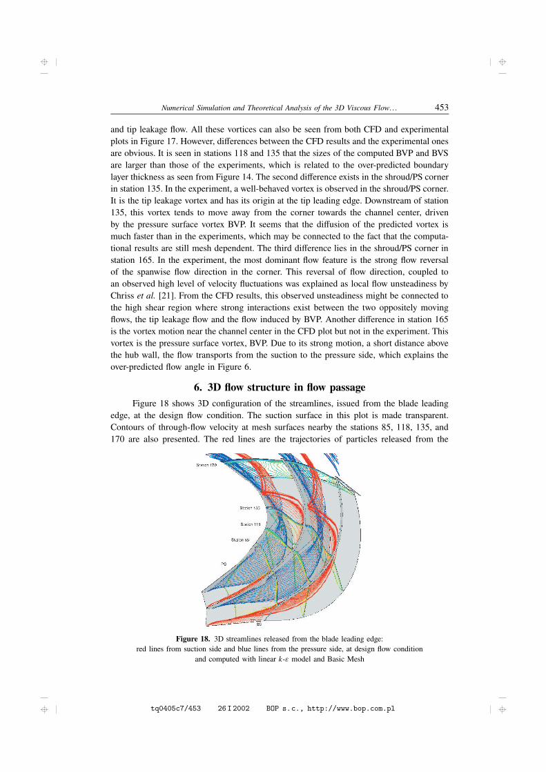
6. 3D flow structure in flow passageFigure 18 shows 3D configuration of the streamlines, issued from the blade leading

edge, at the design flow condition. The suction surface in this plot is made transparent.Contours of through-flow velocity at mesh surfaces nearby the stations 85, 118, 135, and170 are also presented. The red lines are the trajectories of particles released from the

Figure 18. 3D streamlines released from the blade leading edge:red lines from suction side and blue lines from the pressure side, at design flow condition

and computed with linear k-" model and Basic Mesh



suction side leading edge a short distance away from the hub and shroud, while the bluelines are released from the pressure side leading edge. As already observed, all the red linesin the inducer portion migrate upward towards the shroud along the suction surface. Linesclose to the shroud move away from the suction side towards the pressure side just behindstation 118 and reach the mid-pitch region at Station 135. The remaining lines concentrateand migrate into the shroud/SS corner behind Station 135, associated with the BVS motion.They are then tangentially transported away from the corner towards the mid-passage pushedby the tip leakage flow, see the next section for details of the tip flow. These streamlinesthen turn back downward towards the hub in the shroud/PS corner, due to the combinedeffect of the BVP and CV. All these streamlines leave the impeller in the through-flowwake region at station 170. The blue lines along the pressure surface move also upwardsfrom hub to shroud in the inducer portion. The vortex motion associated with the BVPcan be observed in front of station 118 in the shroud/PS corner, in Figure 18, from whichstreamlines near the shroud leave away from the pressure surface. Other lines remain closeto the surface up to station 135. Behind this station, these lines move spirally downstreamunder the red lines, by the effect of a strong BVP. They also pass through the through-flowwake range in station 170.

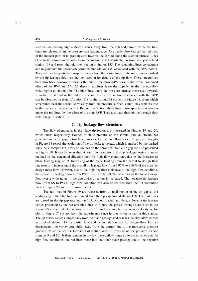
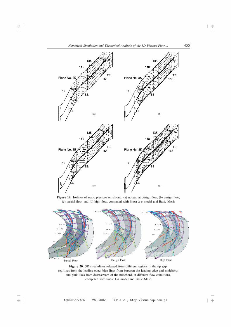
7. Tip leakage flow structureThe flow phenomena in the blade tip region are illustrated in Figures 19 and 20,

which show, respectively, isolines of static pressure on the shroud, and 3D streamlinesgenerated in the tip gap, in two flow passages, for the three flow rates. The pressure troughsin Figure 18 reveal the evolution of the tip leakage vortex, which is marked by the dashedlines. As a comparison, pressure isolines on the shroud without a tip gap are also presentedin Figure 19. It can be seen that at low flow conditions, the tip leakage vortex is moreinclined to the tangential direction than for high flow conditions, due to the increase ofblade loading (Figure 7). Increasing of the blade loading from the partial to design flowrate results in increasing of the overall tip leakage flow from 7.97% to 8.49% of the impellerdesign mass flow. However, due to the high negative incidence in the high flow condition,the overall tip leakage flow (from PS to SS) is only 7.82%, even though the local leakageflow over a wide range in the chordwise direction is increased. The negative tip leakageflow (from SS to PS) at high flow condition can also be realised from the 3D streamlineview in Figure 20 and is discussed below.

The red lines in Figure 19 are released from a small region in the tip gap at theleading edge. The blue lines are issued from the tip gap around station 118. The pink linesare issued in the tip gap near station 135. At both partial and design flows, a tip leakagevortex presented by the red and blue lines in Figure 20, passes through station 85 in theshroud/SS corner, which has also been seen from the computed secondary velocity vectorplot in Figure 17 but not from the experiments since its size is very small at this station.The tip vortex sweeps tangentially over the blade passage and reaches the shroud/PS cornerin front of station 118 for partial flow and behind station 118 for design flow. Furtherdownstream, the vortex core shifts away from the corner, due to the transverse pressuregradient, which causes the formation of isoline loops of pressure on the pressure surface(Figures 9 and 10). It then remains in the low throughflow range up to the impeller exit. Athigh flow conditions, the red lines move into the other blade passage due to the negative



(a) (b)

(c) (d)

Figure 19. Isolines of static pressure on shroud: (a) no gap at design flow, (b) design flow,(c) partial flow, and (d) high flow, computed with linear k-" model and Basic Mesh

Partial Flow Design Flow High Flow

Figure 20. 3D streamlines released from different regions in the tip gap:red lines from the leading edge; blue lines from between the leading edge and midchord;

and pink likes from downstream of the midchord, at different flow conditions,computed with linear k-" model and Basic Mesh



loading in the leading edge portion (Figure 8), resulting in the negative tip leakage flow.The blue lines form the tip leakage vortex, which is originated just upstream of station 85and is located closer to the suction surface than for the lower flow conditions, as seen fromFigure 19. The blue lines move towards the pressure side along the shroud up to station 135,where it contributes to the low energy region in the shroud/PS corner. From this stationto the exit, they remain near the red lines. The pink lines at all three flow conditions areissued in the tip gap near station 135. In the radial portion of the flow passage, behindstation 135, they move away from the suction surface towards the shroud/PS corner. Fromthe shroud/PS corner in front of station 135 for lower flow rates and behind this station forhigher flow rate, they move downstream rejoining the red and blue lines. All lines releasedfrom different chordwise locations leave out the impeller from the low velocity region.

It can then be stated that first signs of the wake are observed, with very small size,from the shroud/SS corner. In the first half of the blade passage, the wake is mainly attributedto the tip leakage flow and tip leakage vortex. Its location shifts towards the suction sidewith the increasing flow rate. Hence the wake moves away from the pressure side with theincreasing flow rate (Figures 14 and 16). In the midway of the blade passage, around station135, low energy fluids from the blade surfaces, associated with the blade surface vortices(BVp and BVs) (Figure 17), and from the tip leakage have merged together, resulting ina large size of the wake region in the pressure/shroud corner. In the remaining blade passage,the radial portion, the secondary flow is dominated by the contribution of the Coriolis force,which is inversely proportional to the meridional velocity. It results in the wake approachingto the suction side with the decreasing flow rate.

8. ConclusionsThe 3D viscous flow in centrifugal compressor impellers has been investigated

theoretically and numerically. The analysis gives an insight into basic mechanisms leadingto the formation of the jet/wake flow structure in centrifugal machines. The main mechanismfor the accumulation of low energy fluid in the shroud area is the radial transport of boundarylayer material along the passage surfaces. Its location results from a balance between theshroud passage vortex, blade surface vortices and tip leakage flows. The balance depends onthe ratio of streamline curvature in the blade-to-blade and meridional surfaces, the Rossbynumber and the ratio of the boundary layer thickness the endwalls and blade surfaces.

The Large Scale Centrifugal Compressor (LSCC) impeller with a vaneless diffuserhas been investigated at three flow rate conditions with EURANUS/TURBO with differentmeshes and turbulence models. An excellent agreement with the available experimental datahas been obtained over a wide region of the flow passage. A grid at order of 600000 pointswas required to get the overall performance, while more points are needed to scrutinise theflow details. To reproduce some micro flow phenomena, unsteady flow computation wasnecessary.

Structures of the 3D flow in the blade passage and the tip region, and their variationswith flow rate as well, were analysed based on the numerical results. The tip vortexoriginating at the tip leading edge sweeps tangentially over the blade passage and reachesthe shroud/PS corner near the midchord. Further downstream, the vortex core shifts awayfrom the corner and remains in the low throughflow area up to the impeller exit. In thefirst half of the blade passage, the low energy fluid area is mainly attributed to the core of



the tip leakage vortex. Its location shifts towards the suction side with the increasing flowrate. In the midway of the blade passage, the low energy fluids from the blade surfaces andthe tip leakage have merged together, resulting in a large size of the wake region in thepressure/shroud corner. In the remaining blade passage, the radial portion, the secondaryflow is dominated by the Coriolis force, resulting in the wake approaching the suction sidewith the decreasing flow rate.

References[1] Langston L S, Nice M L and Hopper R M 1977 J. of Engineering for Power 99 21[2] Chen T G and Goldstein R J 1991 J. of Turbomachinery 114 (4) 776[3] Schulz H D, Gallus H E and Lakshminarayana B 1990 J. of Turbomachinery 112 669[4] Cumpsty N A 1989 Compressor Aerodynamics Longman Scientific and Technical, Essex, England[5] Kang S and Hirsch Ch 1995 J. of Turbomachniery 118 492[6] Kang S 1993 Investigation on the Three-Dimensional Flow Within a Compressor Cascade with and

without Tip Clearance PhD Thesis, Dept. of Fluid Mech., Vrije Universiteit Brussels[7] Eckardt D 1979 Flow Field Analysis of Radial and Bachswept Centrifugal Compressor Impellers,

Part 1: Flow Measurements Using Laser Velocimeter Performance Prediction of Centrifugal Pumpsand Compressors, Gopalakrishnan, ed. ASME Publication, pp. 77–86

[8] Dean R C and Senoo Y 1960 Trans. ASME, Journal of Basic Engineering 82 563[9] Dean R 1971 On the Unresolved Fluid Dynamics of the Centrifugal Compressor in Advanced

Centrifugal Compressors, ASME Publications pp. 1–55[10] Eckardt D 1976 J. of Fluids Engineering 98 390[11] Moore J 1973 J. of Eng. Power 95 205[12] Johnson M W and Moore J 1983 J. of Engineering Power 105 (1) 24[13] Krain H 1988 J. of Turbomachinery 110 122[14] Moore J and Moore J G 1980 Three-Dimensional, Viscous Flow Calculations for Assessing the

Thermodynamic Performance of Centrifugal Compressors – Study of the Eckardt CompressorAGARD-CP-282

[15] Casey W V, Dalbert P and Roth P 1992 J. of Turbomachinery 114 27[16] Denton J D 1986 The Use of a Distributed Body Force to Simulate Viscous Effects in 3D Flow

Calculation ASME Paper 86-GT-144[17] Dawes W N 1988 Development of 1 3D Navier-Stokes for Application to all Types of Turbomachinery

ASME Paper 88-GT-70[18] Dawes W N 1995 Unsteady Flow and Loss Production in Centrifugal and Axial Compressor Stages

AGARD-PEP Paper (37)[19] Hah C and Krain H 1990 J. of Turbomachinery 112 7[20] Johnson M W and Moore J 1983 J. of Engineering Power 105 (1) 33[21] Chriss R M, Hathaway M D and Wood J R 1996 J. of Turbomachinery 118 55[22] Kang S and Hirsch Ch 1999 Effects of Flow Rate on the Development of Three-Dimensional Flow

in NASA LSCC Impeller, Based Numerical Solutions ISABE Paper 99-7225[23] Hirsch Ch, Kang S and Pointet G 1996 A Numerically Supported Investigation on the 3D Flow in

Centrifugal Impellers. Part I: The Validation Base ASME Paper 96-GT-151[24] Hirsch Ch, Kang S and Pointet G 1996 A Numerically Supported Investigation on the 3D Flow in

Centrifugal Impellers. Part II: Secondary Flow Structure ASME Paper 96-GT-152[25] Kang S and Hirsch Ch 1996 Influence of Tip Leakage Flow in Centrifugal Compressor 3rd ISAIF,

Beijing, pp. 186–194[26] Kang S and Hirsch Ch 1999 Numerical Investigation of the Three-Dimensional Flow in MASA

Low-Speed Centrifugal Compressor Impeller 4th ISAIF, Dresden, Germany, pp. 274–284[27] Acosta A J and Bowerman R D 1957 An Experimental Studay of Centrifugal Pump Impellers Trans.

ASME, pp. 1821–1839[28] Van den Braembussche R 1985 Description of Secondary Flow in Radial Flow Machines Published

in Thermodynamics and Fluid Mechanics of Turbomachinery Volume II, Edited by Ucer A S, Stow Pand Hirsch Ch, NATO ASI Series, pp. 665–684



[29] Johnson M W 1978 J. of Engineering Power 100 553[30] Hathaway M D, Chriss R M, Strazisar A J and Wood JR 1995 Laser Anemometer Measurements

of the Three-Dimensional Rotor Flow Field in the NASA Low-Speed Centrifugal Compressor NASATechnical Paper ARL-TR-333

[31] Hirsch Ch, Lacor C, Dener C and Vucinic D 1992 An Integrated CFD System for 3D TurbomachineryApplications AGARD-CP-510

[32] Yang Z and Shih T H 1993 AIAA Journal 31 (7) 1191[33] Khodak A and Hirsch Ch 1996 Second Order Non-Linear k-" Models with Explicit Effect of Curvature

and Rotation Computational Fluid Dynamics’96, Proceeding of the Third ECCOMAS ComputationalFluid Dynamics Conference, pp. 690–696

[34] Hah C, Bryans A C, Moussa Z and Tomsho M E 1988 J. of Turbomachinery 110 303


Documents

numerical simulation and theoretical analysis of the 3d viscous flow